Gain-induced group delay in spontaneous parametric down-conversion

Abstract

Strongly-driven nonlinear optical processes such as spontaneous parametric down-conversion and spontaneous four-wave mixing can produce multiphoton nonclassical beams of light which have applications in quantum information processing and sensing. In contrast to the low-gain regime, new physical effects arise in a high-gain regime due to the interactions between the nonclassical light and the strong pump driving the nonlinear process. Here, we describe and experimentally observe a gain-induced group delay between the multiphoton pulses generated in a high-gain type-II spontaneous parametric down-conversion source. Since the group delay introduces distinguishability between the generated photons, it will be important to compensate for it when designing quantum interference devices in which strong optical nonlinearities are required.

Nonlinear optical processes like spontaneous parametric down-conversion (SPDC) and four-wave mixing have long been used as nonclassical light sources for quantum optics experiments [1, 2, 3, 4, 5, 6]. In these processes, photons from a pump laser interact with a nonlinear medium and scatter into pairs of photons with different energies. Over the years, advances in the ability to manipulate the spatiotemporal properties of the photon pairs [7, 8, 9] have led to improvements in their purity [10], correlation strength [11, 12], and collection efficiency [13]. Photon pair sources have enabled landmark experiments such as the first demonstration of quantum teleportation [14] and the loophole-free violation of Bell’s inequalities [15, 16]. There have also been efforts to increase the strength of the nonlinear interaction beyond the photon pair regime by using pulsed lasers [17, 18, 19], optical cavities [20, 21, 22, 23], and waveguides [24, 25, 26]. When the nonlinear interaction is strong, multiple pump photons scatter coherently into superpositions of many photon pairs, thereby generating squeezed light or twin beams. These light sources have nonclassical properties like reduced electric field fluctuations which can be used for metrology [27] and information processing [28, 29, 19] applications.

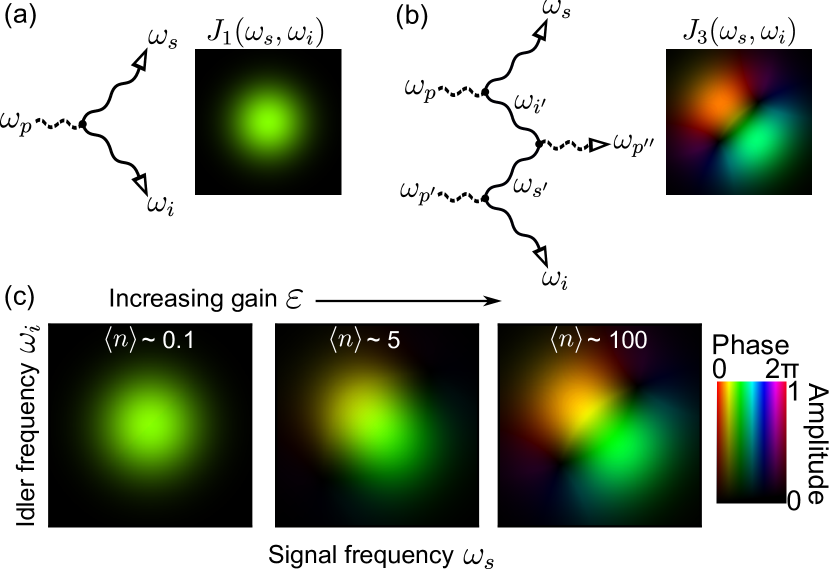
Figure 1: (a) SPDC scattering process to first-order in perturbation theory. Assuming a Gaussian pump and phase-matching function, photon pairs are generated in the joint spectral mode $J_{1}(\omega_{s},\omega_{i})$ with probability amplitude $\varepsilon$. (b) Leading-order correction in the perturbation series describes a more complex scattering process which generates photon pairs in an orthogonal mode $J_{3}(\omega_{s},\omega_{i})$ with probability amplitude $\varepsilon^{3}$. (c) Total joint spectral amplitude is a superposition of both scattering processes as well as higher-order ones [Eq. (4)]. As the gain $\varepsilon$ increases, a linear spectral phase gradient develops along the anti-diagonal axis, leading to a group delay between the generated photons. This delay becomes appreciable when $\braket{n}\gtrsim 1$, where $\braket{n}$ is the average number of photon pairs generated per pump pulse.

Given the huge potential of generating bright nonclassical light, there has been a significant amount of work trying to understand the rich physics that emerges in a strong nonlinear interaction regime, also known as the high-gain regime [30, 31, 32, 33, 34, 35, 36, 37, 38, 39, 40, 41, 42, 43, 44, 45, 46, 47, 48, 49, 50, 51, 52, 53, 54]. For example, pump depletion can lead to correlations between the quantum fields and the classical pump [33, 41, 48, 53]. The three fields can also interact via cross-phase modulation, thereby distorting the spatiotemporal modes of the generated photons [49]. Finally, time-ordering corrections due to the non-commutativity of the Hamiltonian at different times become significant in a high-gain regime [34, 37, 40, 42, 43]. These effects contribute to the challenge of increasing desirable properties such as squeezing despite the ability for experiments to reach very high gains [39, 44, 54].

In this work, we study a gain-induced group delay between the photon pairs generated in SPDC. We experimentally measure the effect using a type-II SPDC source pumped by high-energy ultrashort pulses. When our source generates about a hundred pairs per pump pulse, we measure a group delay between the photons that is on the order of their temporal coherence. We give a physical explanation of this effect both in an interaction picture in terms of scattering processes [Fig. 1] and in a Heisenberg picture in terms of pulse dynamics [Fig. 2].

Under the parametric (i.e. undepleted pump) and rotating-wave approximations, the interaction Hamiltonian describing SPDC is [55]:

$$\begin{split}\hat{\mathcal{H}}(t)&=-\frac{\hbar\varepsilon}{2\pi}\int d\omega_{p}d\omega_{s}d\omega_{i}e^{i\Delta t}\Phi(\omega_{s},\omega_{i},\omega_{p})\\ &\qquad\times\beta(\omega_{p})\hat{a}^{\dagger}(\omega_{s})\hat{b}^{\dagger}(\omega_{i})+\mathrm{h.c.},\end{split}$$ (1)

where $\varepsilon$ is the interaction strength or parametric gain, $\Delta=\omega_{s}+\omega_{i}-\omega_{p}$, and $\hat{a}^{\dagger}(\omega_{s})$ [$\hat{b}^{\dagger}(\omega_{i})$] is the photon creation operator for the signal [idler] mode. The quantities $\Phi(\omega_{s},\omega_{i},\omega_{p})$ and $\beta(\omega_{p})$ are the phase-matching and pump spectral mode functions, respectively. The dynamics of the fields under Eq. (1) are described by the unitary time-evolution operator $\hat{\mathcal{U}}(t,t_{0})=\hat{\mathcal{T}}\exp{[-\frac{i}{\hbar}\int_{t_{0}}^{t}dt^{\prime}\hat{\mathcal{H}}(t^{\prime})]}$ where $\hat{\mathcal{T}}$ is the time-ordering operator. We are interested in obtaining the state of the fields at the end of their interaction, i.e. $\hat{\mathcal{U}}(t\rightarrow\infty,t_{0}\rightarrow-\infty)\equiv\hat{\mathcal{U}}$. If the gain is small ($\varepsilon\ll 1$), the unitary can be expanded to first-order which describes the creation of single photon pairs in the initially vacuum states of the signal and idler modes $\ket{0}_{a}\ket{0}_{b}$:

$$\ket{\Psi}_{ab} =\hat{\mathcal{U}}\ket{0}_{a}\ket{0}_{b}$$ (2)

$$\approx\left(\hat{\mathbbm{1}}-\frac{i}{\hbar}\int_{-\infty}^{\infty}dt\hat{\mathcal{H}}(t)\right)\ket{0}_{a}\ket{0}_{b}$$

$$\approx\ket{0}_{a}\ket{0}_{b}$$

$$\qquad+i\varepsilon\int d\omega_{s}d\omega_{i}J_{1}(\omega_{s},\omega_{i})\hat{a}^{\dagger}(\omega_{s})\hat{b}^{\dagger}(\omega_{i})\ket{0}_{a}\ket{0}_{b},$$

where $J_{1}(\omega_{s},\omega_{i})=\beta(\omega_{s}+\omega_{i})\Phi(\omega_{s},\omega_{i},\omega_{s}+\omega_{i})$ is the normalized joint spectral mode of the photon pairs in a low-gain regime. For many applications, it is desirable to produce photons in a single spectral-temporal mode, in which case the joint mode should be uncorrelated, $J_{1}(\omega_{s},\omega_{i})=f(\omega_{s})g(\omega_{i})$. This can be achieved by satisfying the group velocity condition $v_{s}\leq v_{p}\leq v_{i}$ [8, 56] and employing crystals with apodized periodic poling [9]. The average number of photon pairs generated per pump pulse in the single mode is $\braket{n}=\mathrm{sinh}^{2}(\varepsilon)$.

With increasing $\varepsilon$, one must include higher-order terms in the expansion of $\hat{\mathcal{U}}$. Since $[\hat{\mathcal{H}}(t),\hat{\mathcal{H}}(t^{\prime})]\neq 0$, the Dyson or Magnus series should be used to maintain proper time ordering [37]. As the Dyson expansion does not preserve the correct photon statistics when truncated, we turn to the Magnus expansion [42, 43]:

$$\hat{\mathcal{U}}=\exp{\left(\hat{\Omega}_{1}+\hat{\Omega}_{2}+\hat{\Omega}_{3}+...\right)}.$$ (3)

In particular, $\hat{\Omega}_{1}=-\frac{i}{\hbar}\int_{-\infty}^{\infty}dt\hat{\mathcal{H}}(t)$ while higher-order terms depend on commutators of the Hamiltonian at different times, e.g. $\hat{\Omega}_{2}=\frac{(-i)^{2}}{2\hbar^{2}}\int_{-\infty}^{\infty}dt\int_{-\infty}^{t}dt^{\prime}[\hat{\mathcal{H}}(t),\hat{\mathcal{H}}(t^{\prime})]$. Each term $\hat{\Omega}_{i}$ can be associated with a different type of scattering process which can occur multiple times throughout the unitary evolution as $\hat{\Omega}_{i}$ appears in an exponential in Eq. (3). The first-order term $\hat{\Omega}_{1}$ corresponds to the usual picture of one pump photon scattering into a pair of lower energy photons [Fig. 1(a)]. The second-order term $\hat{\Omega}_{2}$ describes a frequency-conversion process which requires seeding one of the down-converted modes. Since the signal and idler fields are initially in the vacuum state, this term does not contribute, i.e. $\exp{\left(\hat{\Omega}_{2}\right)}\ket{0}_{a}\ket{0}_{b}=\ket{0}_{a}\ket{0}_{b}$. The third order term $\hat{\Omega}_{3}$ describes a scattering process in which two pump photons each produce pairs of down-converted photons followed by the up-conversion of two of the latter photons [Fig. 1(b)]. Since $\hat{\Omega}_{3}$ scales with $\varepsilon^{3}$, the probability of this process occurring is similar to the probability of three photon pairs being generated due to $\hat{\Omega}_{1}$. Thus, $\hat{\Omega}_{3}$ and higher-order terms become appreciable only when multiple photon pairs are generated per pump pulse.

The higher-order terms in the Magnus expansion [Eq. (3)] modify the spectral-temporal properties of the photon pairs:

$$J(\omega_{s},\omega_{i})=\varepsilon J_{1}(\omega_{s},\omega_{i})+\varepsilon^{3}J_{3}(\omega_{s},\omega_{i})+...,$$ (4)

where $J(\omega_{s},\omega_{i})$ is the joint spectral amplitude (JSA) of generating a photon pair. Two of the present authors have developed a Python library, NeedALight, to compute $J(\omega_{s},\omega_{i})$ for arbitrary phase-matching and pump mode shapes [52, 57]. When these functions are Gaussian, we can derive analytic expressions for $J_{1}(\omega_{s},\omega_{i})$ and $J_{3}(\omega_{s},\omega_{i})$ (see the Supplementary Materials [SM] [55]). We find that, even when $J_{1}(\omega_{s},\omega_{i})$ is uncorrelated, the total JSA is no longer uncorrelated due to the presence of a new orthogonal mode $J_{3}(\omega_{s},\omega_{i})$, as has previously been discussed [58, 52]. Another notable feature is that $J_{3}(\omega_{s},\omega_{i})$ contains an imaginary component even when the pump pulse has a uniform spectral phase (i.e. no chirp). This results in a non-trivial joint spectral phase [Fig. 1(c)] that is well approximated by a linear gradient along the anti-diagonal axis, i.e. $\mathrm{arg}[J(\omega_{s},\omega_{i})]\sim\frac{\beta}{2}(\omega_{s}-\omega_{i})$ where $\beta=24\tau\varepsilon^{2}/\sqrt{3\pi}(12+\varepsilon^{2})$ and $\tau$ is the pump pulse duration. As we show in the SM, this causes a temporal group delay of $T=\beta_{0}-\beta$ between the signal and idler photons, where $\beta_{0}=L(v_{s}^{-1}-v_{i}^{-1})/2$ is a gain-independent group delay caused by group-velocity walk-off. Thus, the down-converted photons emerge from the crystal closer in time with increasing $\varepsilon$. Since their coherence time and the group delay both scale with the pump duration $\tau$, the relative size of this effect depends only on the gain $\varepsilon$. In fact, a gain-induced group delay was also discussed in Ref. [36] for the case of a monochromatic pump. Below we provide a physical explanation for its origin, and present an experiment which measures it.

One intuitive but qualitative way to understand the group delay is from the fact that down-converted photons can stimulate further scattering processes. As a result, most photons are created towards the end of the crystal in a high-gain regime [36, 38]. Since they propagate a shorter distance in the crystal, they should suffer less group velocity walk-off. We can connect this explanation to the Magnus expansion. The number of photons generated in the mode $J_{1}(\omega_{s},\omega_{i})$ grows exponentially with $\varepsilon$, as one might expect from stimulated processes. However, there are also photons generated in new modes such as $J_{3}(\omega_{s},\omega_{i})$ which arise due to interactions between the pump and the down-converted photons. For example, the scattering process leading to $J_{3}(\omega_{s},\omega_{i})$ involves the up-conversion of a signal photon $\omega_{s^{\prime}}$ and idler photon $\omega_{i^{\prime}}$ into a pump photon $\omega_{p^{\prime\prime}}$ [Fig. 1(b)]. Due to their different group velocities ($v_{s}\leq v_{p}\leq v_{i}$), for $\omega_{s^{\prime}}$ and $\omega_{i^{\prime}}$ to interact, the production $\omega_{p^{\prime}}\rightarrow(\omega_{s^{\prime}},\omega_{i})$ is more likely to occur before $\omega_{p}\rightarrow(\omega_{s},\omega_{i^{\prime}})$. Thus, while Fig. 1(a) describes a scattering process in which $(\omega_{s},\omega_{i})$ are produced simultaneously with a probability $\sim\varepsilon$, the process in Fig. 1(b) produces $\omega_{i}$ before $\omega_{s}$ with a probability $\sim\varepsilon^{3}$. Since the SPDC interaction is a superposition of both processes (as well as higher order ones), the group delay scales with $\varepsilon^{2}$ to leading order. Note that there would not be a group delay associated with Fig. 1(b) if $v_{s}=v_{i}$.

The interaction between the pump and down-converted light can also be visualized in the Heisenberg picture. By numerically solving the equations of motion [55], we can plot the dynamics of the signal and idler pulses. In a low-gain regime [Fig. 2(a)], these are uniformly amplified throughout the crystal as they travel at their respective group velocities. On average, photons are produced half-way through the crystal [5], leading to a group delay of $\beta_{0}=L(v_{s}^{-1}-v_{i}^{-1})/2$. In contrast, in a high-gain regime [Fig. 2(b)], most amplification occurs towards the end of the crystal. Moreover, there is a larger amplification for temporal components closest to the peak of the pump pulse. As a result, the down-converted pulses tend to become temporally narrower and “stick” to the pump pulse, i.e. their effective group velocities converge to that of the pump with increasing gain. This effect also occurs in classical amplifiers with pulsed gain profiles [59].

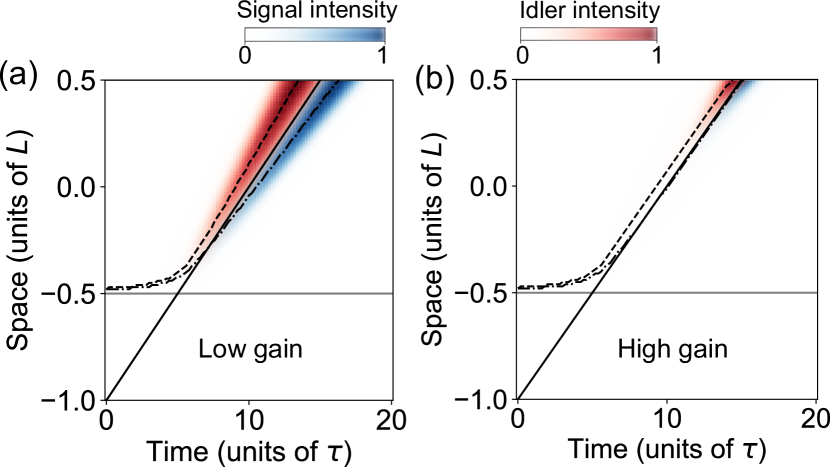
Figure 2: Numerically calculated pulse dynamics in (a) low-gain $\braket{n}\sim 0.1$ and (b) high-gain regime $\braket{n}\sim 100$ using parameters that model the ppKTP source used in the experiment. Black line shows pulse peak for signal (dot dashed), idler (dashed), and pump (continuous). Horizontal grey line indicates the crystal entrance facet. Colormap transparency scales linearly with the pulse energy. Pulses are normalized to their maximal value. $L$ is the crystal length and $\tau$ is the pump pulse duration.

We can measure the group delay using intensity interferometry. As in Hong-Ou-Mandel interferometry, the signal $\hat{a}(\omega_{s})$ and idler $\hat{b}(\omega_{i})$ modes are combined on a balanced beam splitter, $\hat{a}(\omega_{s})\rightarrow(\hat{c}(\omega_{s})+\hat{d}(\omega_{s}))/\sqrt{2}$ and $\hat{b}(\omega_{i})\rightarrow(\hat{c}(\omega_{i})-\hat{d}(\omega_{i}))/\sqrt{2}$. If we consider the contributions to the output state having photons simultaneously in both modes, we find:

$$\ket{\tilde{\Psi}}_{cd}=\mathrm{exp}\Bigg{[}\int d\omega_{s}d\omega_{i}J(\omega_{s},\omega_{i})\times$$ (5)

$$\frac{1}{2}[\hat{c}^{\dagger}(\omega_{i})\hat{d}^{\dagger}(\omega_{s})-\hat{c}^{\dagger}(\omega_{s})\hat{d}^{\dagger}(\omega_{i})]\Bigg{]}\ket{0},$$

where $J(\omega_{s},\omega_{i})$ is the complete JSA, i.e. including all terms in the Magnus expansion. Consider the probability density of measuring a coincidence between a photon with frequency $\omega_{1}$ in mode $c$ and $\omega_{2}$ in mode $d$:

$$\begin{split}\mathrm{pr}(\omega_{1},\omega_{2})&=\left|\braket{0}{\hat{c}(\omega_{1})\hat{d}(\omega_{2})}{\tilde{\Psi}_{cd}}\right|^{2}\\ &=\frac{1}{4}|J(\omega_{1},\omega_{2})-J(\omega_{2},\omega_{1})|^{2},\end{split}$$ (6)

which is a projection onto the anti-symmetric component of the JSA. If the signal and idler photons are symmetric (i.e. indistinguishable) in amplitude, $|J(\omega_{1},\omega_{2})|=|J(\omega_{2},\omega_{1})|$, then we find:

$$\mathrm{pr}(\omega_{1},\omega_{2})=\frac{1}{2}|J(\omega_{1},\omega_{2})|^{2}\left(1-\cos{[\tfrac{T}{2}(\omega_{1}-\omega_{2})]}\right)$$ (7)

where $\mathrm{arg}\left[J(\omega_{1},\omega_{2})\right]=\tfrac{T}{2}(\omega_{1}-\omega_{2})$ is a linear spectral phase gradient due to a group delay of $T$ between the photons. Thus, the single-pair coincidence probability is an interferogram whose fringe pattern can be related to the group delay $T$ [60, 61, 62, 63].

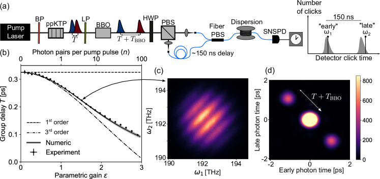
Figure 3: (a) Experimental setup. BP: bandpass filter, LP: longpass filter, HWP: half-wave plate, PBS: polarizing beam splitter, SNSPD: superconducting nanowire single photon detector. BBO crystal is used as a linear optical element to increase the group delay between the signal and idler photons produced by the ppKTP. Detection time of the photons is related to their frequency due to the dispersive fiber. (b) Group delay $T$ measured as a function of parametric gain $\varepsilon$. Horizontal dashed line is an analytic model limited to the first-order Magnus term $\hat{\Omega}_{1}$, in which case the expected group delay is simply the group velocity walk-off $\beta_{0}=L(v_{s}^{-1}-v_{i}^{-1})/2$. Dotted-dashed line is $T=\beta_{0}-24\tau\varepsilon^{2}/\sqrt{3\pi}(12+\varepsilon^{2})$ based on Magnus expansion up to $\hat{\Omega}_{3}$. Shaded black curve is the numerical model NeedALight [57], where shaded region represents 95% confidence interval. (c) Example of a spectrally-resolved coincidence histogram $N(\omega_{1},\omega_{2})$ measured when $\varepsilon=1.407(3)$. (d) Fourier transform of $N(\omega_{1},\omega_{2})$. Colorbar shows number of events per bin collected in five minutes.

In practice, it is challenging to measure Eq. (7) in a high-gain regime due to optical losses and a lack of spectrally-resolving photon-number-resolving detectors. If $\ket{\tilde{\Psi}}_{cd}$ is attenuated to the single-photon level such that it can be measured with click detectors, the correlations between photon pairs become muddled. However, spectrally-resolved coincidences still reveal an interference pattern which can be used to determine the group delay between the two incident pulses [63]. In the SM, we show that after attenuation:

$$\mathrm{pr}(\omega_{1},\omega_{2})\propto[j(\omega_{1})j(\omega_{2})]^{2}(1-\mathcal{V}\cos{[\tfrac{T}{2}(\omega_{1}-\omega_{2})]})$$ (8)

where $j(\omega)=\int d\omega^{\prime}|J(\omega,\omega^{\prime})|=\int d\omega^{\prime}|J(\omega^{\prime},\omega)|$ is the marginal spectral amplitude of the signal and idler photons. The interference visibility $\mathcal{V}\leq 1/3$ is a phenomenological parameter that accounts for the signal and idler thermal statistics, dark counts, and any other effect which reduces the fringe contrast.

The experimental setup is shown in Fig 3(a). The pump laser is an optical parametric amplifier (LightConversion Orpheus-HP) that generates 180 fs pulses (center wavelength 779 nm) at a 200 kHz repetition rate. The pump bandwidth is set to 5.37(5) nm full-width-at-half-maximum using a pair of bandpass filters. The SPDC source uses a group-velocity matching condition, as in Refs. [64, 65, 66]. We focus the pump into a 2-mm-long periodically poled potassium titanyl phosphate (ppKTP) crystal to produce collinear and orthogonally-polarized degenerate photon pairs with center wavelength of 1558 nm (192 THz). The photon pairs are mixed by a half-wave plate and spatially-separated by a polarizing beam splitter (PBS). The vertical output of the PBS is delayed by about 150 ns and recombined with the horizontal output such that both modes can be detected by the same detector. To achieve spectrally-resolved single photon detection, we use a long dispersive fiber (group delay dispersion 1.033 ns/nm, insertion loss 3.3 dB) and a superconducting nanowire (jitter 0.1 ns) to implement a time-of-flight spectrometer [67]. Using a Klyshko measurement [68], we estimate the total (including detection) efficiency of the setup to be $\eta=7(1)$ % in both outputs of the PBS. This efficiency provides sufficient attenuation to measure $\mathrm{pr}(\omega_{1},\omega_{2})$ [Eq. (8)] even at the highest gain reached in our experiment ($\varepsilon\sim 3$, $\braket{n}\sim 100$).

We scan the pump power from 0 to 60 mW and record timetags of coincidence events where at least one photon was detected in both outputs of the PBS. The timetags are converted to a frequency and then placed into a histogram with 30 GHz wide bins, $N(\omega_{1},\omega_{2})\propto\mathrm{pr}(\omega_{1},\omega_{2})$ [Fig. 3(c)]. The group delay is measured by taking a Fourier transform of the $N(\omega_{1},\omega_{2})$ and determining the distance between the center peak and the sidebands [Fig. 3(d)]. In order to facilitate measuring this distance, we insert a 2-mm-long $\alpha$-BBO crystal which increases the group delay by an offset $T_{\mathrm{BBO}}$. The offset value $T_{\mathrm{BBO}}=0.833$ ps is then subtracted from the distance to obtain the group delay $T$. The values of $T$ measured at different gains $\varepsilon$ are plotted in Fig. 3(b). This is the main result of the paper. At low gain, we find that $T=0.327(7)$ ps which is in agreement with the expected value of $\beta_{0}=L(v_{s}^{-1}-v_{i}^{-1})/2=0.325$ ps given by the birefringent walk-off in the ppKTP [69]. With increasing gain, the signal and idler photons exit the crystal closer in time, as expected. The group delay agrees with the analytic third-order Magnus expansion until $\epsilon\sim 1$. Beyond this point, we find good agreement with a numerical model which solves the Heisenberg equations of motion using NeedALight [57]. All its parameters, including the gain $\varepsilon$, are determined from independent measurements [55].

In summary, we demonstrated that photon pairs generated by spontaneous parametric down-conversion exhibit a gain-induced group delay. While our discussion focused on a bulk crystal pumped by ultrashort pulses, we expect the group delay to affect a broad range of photon pair and squeezed light sources. For instance, the Hamiltonian in Eq. (1) also describes spontaneous four-wave mixing [42] which is often used in integrated circuits or optical fibers. Furthermore, the group delay will also affect sources pumped by longer pulses or even continuous-wave light [36]. Our results show that the joint spectral amplitude is not simply determined by the product of the phase-matching and pump mode functions in a high-gain regime. This regime is becoming increasingly relevant for applications like photonic quantum computing [29], Gaussian boson sampling [70, 66, 71, 19], interferometry [72, 73, 74, 75], and quantum frequency conversion [76, 77, 78]. In some of these applications, the group delay introduces distinguishability between the generated photons which can severely reduce the performance of the device. For example, in a nonlinear interferometer, the signal and idler pulses generated by the first parametric amplifier must be temporally overlapped in the second one to maximize the interference visibility [74]. With bulk optics, it is relatively straightforward to compensate for the group delay using translation stages. However, the delay may pose complications when designing quantum interference circuits integrated into chips [79, 80, 26, 23, 81].

Supplemental material

.1 Hamiltonian

We start by considering propagation in a quasi-one-dimensional geometry with three beams that we label signal (s), idler (i), and pump (p). Each beam is characterized by a central frequency $\bar{\omega}_{\mu}$, a wavevector $\bar{k}_{\mu}$ ($\{s,i,p\}\ni\mu$), and a dispersion relation

$$\underbrace{k_{\mu}-\bar{k}_{\mu}}_{\equiv\delta k_{\mu}}=\frac{1}{v_{\mu}}\underbrace{(\omega_{\mu}-\bar{\omega}_{\mu})}_{\equiv\delta\omega_{\mu}},$$ (S9)

where $v_{\mu}$ is the group velocity of beam $\mu$ which is assumed to be constant over the range of frequencies involved. We assume that higher order dispersion terms have a negligible effect given the (narrow) frequency support of the beams in considerations. As we are interested in type-II SPDC, we assume that the central frequencies and wavevectors satisfy energy conservation and (quasi-)phase matching

$$\bar{\omega}_{p}-\bar{\omega}_{s}-\bar{\omega}_{i}= 0,$$ (S10)

$$\bar{k}_{p}-\bar{k}_{s}-\bar{k}_{i}= 0\ (\text{or }=\pm\frac{2\pi}{\Lambda}\text{if quasi-phase-matching}).$$ (S11)

For the quasi-phase matching case, $\Lambda$ is the poling period. The free (i.e. linear) Hamiltonian of the beams is given by

$$\hat{\mathcal{H}}_{\text{L}} =\sum_{\{s,i,p\}\ni\mu}\int dk\hbar\omega_{\mu}(k_{\mu})\hat{a}^{\dagger}_{\mu}(k_{\mu})\hat{a}_{\mu}(k_{\mu})$$ (S12)

$$=\sum_{\{s,i,p\}\ni\mu}\int dz\hbar\left[\bar{\omega}_{\mu}\hat{\psi}_{\mu}^{\dagger}(z)\hat{\psi}_{\mu}(z)-\tfrac{i}{2}v_{\mu}\left\{\hat{\psi}_{\mu}^{\dagger}(z,t)\frac{\partial\hat{\psi}_{\mu}(z,t)}{\partial z}-\frac{\partial\hat{\psi}_{\mu}^{\dagger}(z,t)}{\partial z}\hat{\psi}_{\mu}(z,t)\right\}\right]$$

where we have introduced the bosonic creation and annihilation operators which satisfy

$$[\hat{a}_{i}(k),\hat{a}^{\dagger}_{j}(k^{\prime})]=\delta(k-k^{\prime})\delta_{i,j},$$ (S13)

and all others commutation relations are zero. Similarly, we expressed the Hamiltonian in terms of the field operators which are defined as

$$\hat{\psi}_{\mu}(z)=\int\frac{dk}{\sqrt{2\pi}}\hat{a}_{\mu}(k)e^{i(k-\bar{k}_{\mu})z}.$$ (S14)

Under the rotating-wave approximation, we keep only the resonant terms for the nonlinear portion of the Hamiltonian. Doing so, we find

$$\hat{\mathcal{H}}_{\text{NL}}=-\hbar\int dz\Bigl{\{}\zeta_{s,i,p}g(z)\hat{\psi}^{\dagger}_{s}(z)\hat{\psi}^{\dagger}_{i}(z)\hat{\psi}_{p}(z)+\frac{1}{2}\zeta_{p}h(z)\hat{\psi}^{\dagger}_{p}(z)^{\dagger}\hat{\psi}^{\dagger}_{p}(z)\hat{\psi}_{p}(z)\hat{\psi}_{p}(z)$$

$$+\zeta_{s}h(z)\hat{\psi}^{\dagger}_{p}(z)\hat{\psi}_{p}(z)\hat{\psi}^{\dagger}_{s}(z)\hat{\psi}_{s}(z)+\zeta_{i}h(z)\hat{\psi^{\dagger}}_{p}(z)\hat{\psi}_{p}(z)\hat{\psi}^{\dagger}_{i}(z)\hat{\psi}_{i}(z)+\text{h.c.}\Bigr{\}}.$$ (S15)

In the first term, responsible for pair creation, we have $\zeta_{s,i,p}=\sqrt{\frac{\hbar\bar{\omega}_{s}\bar{\omega}_{i}\bar{\omega}_{p}}{2\epsilon_{0}\bar{n}_{s}\bar{n}_{i}\bar{n}_{p}A_{s,i,p}}}\bar{\chi}_{2}$, where $\bar{n}_{j}$ is the index of refraction of beam $j$ at $\bar{\omega}_{j}$, $\epsilon_{0}$ is the permittivity of vacuum, and $A_{s,i,p}$ is a characteristic area describing the region over which the interaction occurs [50]. The function $g(z)$ is the poling function which takes on the values $g(z)=0$ where the nonlinearity is absent and either $+1$ or $-1$ depending on the orientation of the nonlinear medium. As an example, for quasi-phase matching, $g(z)$ would be an alternating function of $\pm 1$ over small intervals of length $\Lambda$. The next three terms are responsible for self- and cross-phase modulation of the beams. The function $h(z)$ is a square function which is $+1$ where the nonlinearity is present and $0$ otherwise. For the self-phase modulation of the pump, we have $\zeta_{p}=\frac{3}{4\epsilon_{0}}\left(\frac{\hbar\bar{\omega}_{p}^{2}}{\bar{n}_{p}^{2}\sqrt{A_{p}}}\right)\bar{\chi}_{3}$ and for the cross-phase modulation we have $\zeta_{\mu}=\frac{3}{2\epsilon_{0}}\left(\frac{\hbar\bar{\omega}_{p}\bar{\omega}_{\mu}}{\bar{n}_{p}\bar{n}_{\mu}\sqrt{A_{\mu}}}\right)\bar{\chi}_{3}$ where $\mu=s,i$. Again, $A_{j}$ for $\{s,i,p\}\ni j$ is a characteristic area describing the area over which the self- and cross-phase modulation interactions occur.

We can then construct an effective Hamiltonian for our model which we use to obtain the Schrödinger equation satisfied by the evolution operator

$$i\hbar\frac{d}{dt}\hat{\mathcal{U}}(t,t_{0})=\hat{\mathcal{H}}_{\text{eff}}\hat{\mathcal{U}}(t,t_{0})=\left(\hat{\mathcal{H}}_{\text{L}}+\hat{\mathcal{H}}_{\text{NL}}\right)\hat{\mathcal{U}}(t,t_{0}),$$ (S16)

where at the initial time $t_{0}$, $\hat{\mathcal{U}}(t_{0},t_{0})=\hat{\mathbb{1}}$ with $\hat{\mathbb{1}}$ being the identity operator. With the evolution operator in hand, we can now consider how initial states evolve by either evaluating $\ket{{\psi}(t)}=\hat{\mathcal{U}}(t,t_{0})\ket{{\psi}(t_{0})}$ or by solving the Heisenberg equations of motion for the Heisenberg field operators $\hat{\psi}_{j}(z,t)=\hat{\mathcal{U}}^{\dagger}(t,t_{0})\hat{\psi}_{j}(z,t_{0})\hat{\mathcal{U}}(t,t_{0})$.

The state that we are interested in evolving is a product of vacuum for the signal and idler beams and a strong coherent state for the pump:

$$\ket{\Psi(t_{0})}=\exp\left(\int dzf_{p}(z)\hat{\psi}^{\dagger}_{p}(z)-\text{h.c.}\right)\ket{\text{vac}}=\exp\left(\int dk\alpha_{p}(k)\hat{a}^{\dagger}_{p}(k)-\text{h.c.}\right)\ket{\text{vac}},\ \ket{\text{vac}}=\ket{\text{vac}_{p}}\otimes\ket{\text{vac}_{s}}\otimes\ket{\text{vac}_{i}}$$ (S17)

where $\ket{\text{vac}}$ is the three-beam vacuum state, and $\exp\left(\int dzf_{p}(z)\psi_{p}(z)^{\dagger}-\text{h.c.}\right)$ is a displacement operator. We will assume that the nonlinear region lies in the region $-L/2<z<L/2$ , where $L$ is the length of the crystal. Moreover, we assume that at time $t_{0}$, the pump envelope function has not entered yet entered the crystal such that $\int_{-L/2}^{L/2}dz|f_{p}(z)|^{2}\approx 0$.

.2 Heisenberg dynamics

From our effective Hamiltonian, we find that the Heisenberg equation for the pump field operator is

$$\left(\frac{\partial}{\partial t}+v_{p}\frac{\partial}{\partial z}+i\bar{\omega}_{p}\right)\hat{\psi}_{p}(z,t)=i\zeta_{p}h(z)\hat{\psi}_{p}(z,t)^{\dagger}\hat{\psi}_{p}(z,t)\hat{\psi}_{p}(z,t)+\text{back action terms},$$ (S18)

where the “back action terms” are interaction terms which contain the signal and idler field operators. We make the undepleted-classical pump approximation such that $\hat{\psi}_{p}(z,t)\rightarrow\langle\hat{\psi}_{p}(z,t)\rangle$ and assume that the number of pump photons remains unchanged. Under these assumptions, we can ignore these back action terms, and obtain a solution for the mean pump field

$$\langle\hat{\psi}_{p}(z,t)\rangle=f_{p}(z-v_{p}(t-t_{0}))e^{i\bar{\omega}_{p}(t-t_{0})+i\theta(z,t)}$$ (S19)

where

$$\langle\hat{\psi}_{p}(z,t_{0})\rangle=f_{p}(z)$$ (S20)

is the spatial pump envelope function at time $t_{0}$ [Eq. (S17)] and the phase accumulated by self-phase modulation is

$$\theta(z,t)=|f_{p}(z-v_{p}(t-t_{0}))|^{2}\int_{t_{0}}^{t}dt^{\prime}\zeta_{p}h(z-v_{p}(t-t^{\prime})).$$ (S21)

Having a solution for the mean pump field, we now consider the Heisenberg equations of motion for the signal and idler fields

$$\left(\frac{\partial}{\partial t}+v_{s}\frac{\partial}{\partial z}+i\bar{\omega}_{s}\right)\hat{\psi}_{s}(z,t) =i\zeta_{s,i,p}g(z)\langle\hat{\psi}_{p}(z,t)\rangle\hat{\psi}^{\dagger}_{i}(z,t)+i\zeta_{s}h(z)|\langle\hat{\psi}_{p}(z,t_{0})\rangle|^{2}\hat{\psi}_{s}(z,t)$$ (S22)

$$\left(\frac{\partial}{\partial t}+v_{i}\frac{\partial}{\partial z}+i\bar{\omega}_{i}\right)\hat{\psi}^{\dagger}_{i}(z,t) =-i\zeta^{*}_{s,i,p}g(z)\langle\hat{\psi}_{p}(z,t)\rangle\hat{\psi}_{s}(z,t)-i\zeta^{*}_{i}h(z)|\langle\hat{\psi}_{p}(z,t_{0})\rangle|^{2}\hat{\psi}^{\dagger}_{i}(z,t).$$ (S23)

We solve these equations via two different, yet similar, methods which are all included in the Python package NeedALight. For the first method, we follow the steps of Ref. [49, 58] and Fourier transform into frequency space. Doing so gives us integro-differential equations in ($z,\omega$) space. The terms on the right-hand side of the equations become convolutions. We solve numerically by discretizing the frequencies onto a grid of $N$ points and approximating the integrals as sums which give rise to matrix equations of motion. For the second method, we follow the steps of Ref. [82] and Fourier transform into momentum space which gives us equations of motion in ($k,t$) space. Again, the terms on the right-hand side become convolutions. Similarly, we solve numerically by discretizing the momenta on a grid of $N$ points and approximating the integrals as sums.

Once the solutions are obtained, we can evaluate certain quantities directly in the chosen space (e.g. the JSA) or Fourier transform back into ($z,t$) to see how the energy densities evolve.

.3 Magnus Expansion

By numerically solving the Heisenberg equations of motion, we can study how the signal and idler energy densities evolve as a function of time [Fig. 2]. However, it is worth also considering the problem in the Schrödinger picture which can be solved analytically under certain simplifying assumptions (which we explicitly mention below). In this picture, the solution to Eq. (S16) is

$$\hat{\mathcal{U}}(t,t_{0})=\hat{\mathcal{T}}\exp\left[-\frac{i}{\hbar}\int_{t_{0}}^{t}dt^{\prime}\left(\hat{\mathcal{H}}_{\text{L}}+\hat{\mathcal{H}}_{\text{NL}}(t^{\prime})\right)\right],$$ (S24)

where $\hat{\mathcal{T}}$ denotes the time-ordering operator. To obtain an approximate analytic expression for $\hat{\mathcal{U}}(t,t_{0})$, one usually resorts to perturbative expansions such as the Magnus series. To do so, we first move into the interaction picture and define the interaction evolution operator

$$\hat{\mathcal{U}}_{I}(t,t_{0})=e^{\frac{i}{\hbar}\hat{\mathcal{H}}_{\text{L}}(t-t_{0})}\hat{\mathcal{U}}(t,t_{0}).$$ (S25)

This operator obeys the new Schrödinger equation

$$i\hbar\frac{d}{dt}\hat{\mathcal{U}}_{I}(t,t_{0})=\hat{\mathcal{H}}_{\text{I}}(t)\hat{\mathcal{U}}_{I}(t,t_{0}),$$ (S26)

where

$$\hat{\mathcal{H}}_{\text{I}}(t)=e^{\frac{i}{\hbar}\hat{\mathcal{H}}_{\text{L}}(t-t_{0})}\hat{\mathcal{H}}_{\text{NL}}(t)e^{-\frac{i}{\hbar}\hat{\mathcal{H}}_{\text{L}}(t-t_{0})}.$$ (S27)

We can write the formal solution of the interaction-picture Schrödinger equation again in terms of time-ordered exponential

$$\hat{\mathcal{U}}_{I}(t,t_{0})=\hat{\mathcal{T}}\exp\left[-\frac{i}{\hbar}\int_{t_{0}}^{t}dt^{\prime}\hat{\mathcal{H}}_{I}(t^{\prime})\right].$$ (S28)

This allows us to focus solely on the nonlinear Hamiltonian which gives us the interesting dynamics. The evolution operator in Eq. (S28) can be expanded according to a Magnus series:

$$\hat{\mathcal{U}}_{I}(t,t_{0})=\exp{\left[\hat{\Omega}_{1}(t,t_{0})+\hat{\Omega}_{2}(t,t_{0})+\hat{\Omega}_{3}(t,t_{0})+...\right]}$$ (S29)

where

$$\hat{\Omega}_{1}(t,t_{0}) =\frac{-i}{\hbar}\int_{t_{0}}^{t}dt^{\prime}\hat{\mathcal{H}}_{I}(t^{\prime})$$ (S30)

$$\hat{\Omega}_{2}(t,t_{0}) =\frac{(-i)^{2}}{2\hbar^{2}}\int_{t_{0}}^{t}dt^{\prime}\int_{t_{0}}^{t^{\prime}}dt^{\prime\prime}[\hat{\mathcal{H}}_{I}(t^{\prime}),\hat{\mathcal{H}}_{I}(t^{\prime\prime})]$$ (S31)

$$\hat{\Omega}_{3}(t,t_{0}) =\frac{(-i)^{3}}{6\hbar^{3}}\int_{t_{0}}^{t}dt^{\prime}\int_{t_{0}}^{t^{\prime}}dt^{\prime\prime}\int_{t_{0}}^{t^{\prime\prime}}dt^{\prime\prime\prime}\left([\hat{\mathcal{H}}_{I}(t^{\prime}),[\hat{\mathcal{H}}_{I}(t^{\prime\prime}),\hat{\mathcal{H}}_{I}(t^{\prime\prime\prime})]]+[[\hat{\mathcal{H}}_{I}(t^{\prime}),\hat{\mathcal{H}}_{I}(t^{\prime\prime})],\hat{\mathcal{H}}_{I}(t^{\prime\prime\prime})]\right)$$ (S32)

with $t_{0}<t^{\prime\prime}<t^{\prime}<t$. Following the derivations in Refs. [42, 43], we can arrive at analytic expressions for $\hat{\Omega}_{i}(t,t_{0})$ for $i\leq 3$ by making a number of simplifying assumptions.

(i) Firstly, we neglect higher-order nonlinear effects such as cross-phase modulation and self-phase modulation. As such, the interaction Hamiltonian takes the simpler form

$$\hat{\mathcal{H}}_{I}(t)=-\frac{\hbar\zeta_{s,i,p}}{(2\pi)^{3/2}}\int dk_{s}dk_{i}dk_{s}\left[\int_{-L/2}^{L/2}dzg(z)e^{-i(\delta k_{s}+\delta k_{i}-\delta k_{p})z}\right]\hat{a}_{s}^{\dagger}(k_{s})\hat{a}_{i}^{\dagger}(k_{i})\alpha_{p}(k_{p})e^{i\left(\delta\omega_{s}+\delta\omega_{i}-\delta\omega_{p}\right)(t-t_{0})}+\text{h.c.}$$ (S33)

where $\alpha_{p}(k_{p})=\langle\hat{a}_{p}(k_{p})\rangle$ is the momentum space pump envelope function. It is convenient to work in terms of frequency rather than momenta, as such, we make a change of variable and recall that $\hat{a}_{j}(k_{j})\rightarrow\hat{a}_{j}(\omega_{j})\cdot\sqrt{\frac{\partial\omega_{j}}{\partial k_{j}}}=\hat{a}_{j}(\omega_{j})\sqrt{v_{j}}$ to arrive at

$$H_{I}(t) =-\hbar C^{\prime}\int d\omega_{s}d\omega_{i}d\omega_{p}\Phi(\Delta k)\beta_{p}(\omega_{p})\hat{a}_{s}^{\dagger}(\omega_{s})\hat{a}_{i}^{\dagger}(\omega_{i})e^{i(\omega_{s}+\omega_{i}-\omega_{p})(t-t_{0})}+\text{h.c.}$$ (S34)

$$C^{\prime} =\bar{\chi}_{2}\sqrt{\frac{N\bar{\omega}_{p}\bar{\omega}_{s}\bar{\omega}_{i}}{2\varepsilon_{0}\bar{n}_{s}\bar{n}_{i}\bar{n}_{p}A(2\pi)^{3}v_{p}v_{s}v_{i}}},$$ (S35)

where $\beta_{p}(\omega_{p})=\alpha_{p}(\omega_{p})/\sqrt{N}=\braket{\hat{a}_{p}(\omega_{p})}/\sqrt{N}$ is the normalized spectral content of the pump and we have defined the phase-matching function

$$\Phi(\Delta k)=\int_{-L/2}^{L/2}dzg(z)e^{-i\Delta kz}.$$ (S36)

where $\Delta k\equiv\delta k_{s}(\omega_{s})+\delta k_{i}(\omega_{i})-\delta k_{p}(\omega_{p})$ is the wavevector mismatch.

(ii) Secondly, we assume both the pump spectral mode and phase-matching functions can be approximated by Gaussians. The pump mode is given by

$$\beta_{p}(\omega_{p})=\sqrt[4]{\frac{2}{\pi}}\sqrt{\tau}\exp(-\tau^{2}(\omega_{p}-\bar{\omega}_{p})^{2}).$$ (S37)

For the phase-matching function, we perform the integral in Eq. (S36) with $g(z)\equiv 1$ to obtain

$$\begin{split}\Phi(\Delta k)&=\mathrm{sinc}\left(\frac{\Delta kL}{2}\right)\\ &\approx\exp\left[-\gamma\left(\frac{\Delta kL}{2}\right)^{2}\right],\end{split}$$ (S38)

where $\gamma\approx 0.193$ is the optimal value to approximate the sinc function. In practice, an apodized poling function $g(z)$ can be used to obtain a Gaussian phase matching function [9].

We now begin by computing $\hat{\Omega}_{1}(t,t_{0})$. We take $t_{0}\to-\infty$ and $t\to\infty$ (in practice this just means $t_{0}$ before the pump enters the nonlinear region and $t$ after it exits it) in which case $\int_{-\infty}^{\infty}dt^{\prime}e^{i(\omega_{s}+\omega_{i}-\omega_{p})t^{\prime}}=2\pi\delta(\omega_{s}+\omega_{i}-\omega_{p})$. Using this result we can write

$$\begin{split}\hat{\Omega}_{1}(t,t_{0})=&-\frac{i}{\hbar}\int_{t_{0}}^{t}dt^{\prime}H_{I}(t^{\prime})\\ &=2\pi iC^{\prime}\int d\omega_{s}d\omega_{i}\Phi(\Delta k)\beta_{p}(\omega_{s}+\omega_{i})\hat{a}_{s}^{\dagger}(\omega_{s})\hat{a}^{\dagger}_{i}(\omega_{i})+\text{h.c.}\end{split}$$ (S39)

Expanding the wavevector mismatch $\Delta k$, we find

$$\sqrt{\gamma}\Delta kL/2=\underbrace{\frac{\sqrt{\gamma}L}{2}\left(\frac{1}{v_{s}}-\frac{1}{v_{p}}\right)}_{\equiv\eta_{s}}\underbrace{(\omega_{s}-\bar{\omega}_{s})}_{\equiv\delta\omega_{s}}+\underbrace{\frac{\sqrt{\gamma}L}{2}\left(\frac{1}{v_{i}}-\frac{1}{v_{p}}\right)}_{\equiv\eta_{i}}\underbrace{(\omega_{i}-\bar{\omega}_{i})}_{\equiv\delta\omega_{i}}$$ (S40)

which allows us to re-write Eq. (S39) as

$$\begin{split}\hat{\Omega}_{1}(t,t_{0})&=2\pi iC^{\prime}\sqrt[4]{\frac{2}{\pi}}\sqrt{\tau}\int d\omega_{s}d\omega_{i}\exp\left[-(\eta_{s}^{2}+\tau^{2})[\delta\omega_{s}]^{2}-(\eta_{i}^{2}+\tau^{2})[\delta\omega_{i}]^{2}-2(\tau^{2}+\eta_{s}\eta_{i})\delta\omega_{s}\delta\omega_{i}\right]\hat{a}_{s}^{\dagger}(\omega_{s})\hat{a}_{i}^{\dagger}(\omega_{i})+\mathrm{h.c.}\end{split}$$ (S41)

(iii) Thirdly, we will assume that $\tau^{2}+\eta_{s}\eta_{i}=0$, meaning that there are no correlations between signal and idler to first-order in perturbation. Moreover, we will take $\eta_{s}=-\eta_{i}=\pm\tau$. These conditions can be met using group velocity matching. We then find:

$$\hat{\Omega}_{1}(t,t_{0})=2\pi iC^{\prime}\sqrt[4]{\frac{2}{\pi}}\sqrt{\frac{\pi}{4\tau}}\int d\omega_{s}d\omega_{i}f_{0}(\delta\omega_{s})f_{0}(\delta\omega_{i})\hat{a}_{s}^{\dagger}(\omega_{s})\hat{a}_{i}^{\dagger}(\omega_{i})+\text{h.c.}$$ (S42)

where $f_{0}(\delta\omega_{s,i})=\sqrt[4]{\frac{1}{\pi}}\sqrt{2\tau}\exp(-2\tau^{2}\delta\omega_{s,i}^{2})$ is a normalized function such that $\int d\omega_{s,i}|f_{0}(\delta\omega_{s,i})|^{2}=1$. Defining $\varepsilon=2\pi C^{\prime}\sqrt[4]{\frac{2}{\pi}}\sqrt{\frac{\pi}{4\tau}}$, we arrive at the first-order Magnus term

$$\hat{\Omega}_{1}(t,t_{0})=i\varepsilon\int d\omega_{s}d\omega_{i}J_{1}(\omega_{s},\omega_{i})\hat{a}_{s}^{\dagger}(\omega_{s})\hat{a}_{i}^{\dagger}(\omega_{i})+\text{h.c.}$$ (S43)

with a first-order joint spectral mode

$$J_{1}(\omega_{s},\omega_{i})=f_{0}(\delta\omega_{s})f_{0}(\delta\omega_{i}).$$ (S44)

We now derive the expression for the next leading order correction to the joint spectral amplitude. If we truncate Eq. (S29) to third order in the Magnus expansion, we can use the Zassenhaus and Baker-Campbell-Hausdorff identities to arrive at

$$\hat{\mathcal{U}}_{I}(t,t_{0})\approx\exp{\left[\hat{\Omega}_{1}(t,t_{0})+\hat{\Omega}_{3}(t,t_{0})-\frac{1}{2}[\hat{\Omega}_{1}(t,t_{0}),\hat{\Omega}_{2}(t,t_{0})]\right]}\exp{\left[\hat{\Omega}_{2}(t,t_{0})\right]}.$$ (S45)

We note that $\exp{\left[\hat{\Omega}_{2}(t,t_{0})\right]}\ket{0}_{a}\ket{0}_{b}=\ket{0}_{a}\ket{0}_{b}$. Following a lengthy derivation which can be found in the Supplementary Materials of Ref. [43] or in Ref. [50], one can show that:

$$\begin{split}\hat{\Omega}_{3}(t,t_{0})&=i\varepsilon^{3}\int d\omega_{s}d\omega_{i}L_{3}(\omega_{s},\omega_{i})\hat{a}_{s}^{\dagger}(\omega_{s})\hat{a}_{i}^{\dagger}(\omega_{i})+\text{h.c.},\\ \frac{1}{2}[\hat{\Omega}_{1}(t,t_{0}),\hat{\Omega}_{2}(t,t_{0})]&=-\varepsilon^{3}\int d\omega_{s}d\omega_{i}K_{3}(\omega_{s},\omega_{i})\hat{a}_{s}^{\dagger}(\omega_{s})\hat{a}_{i}^{\dagger}(\omega_{i})+\text{h.c.}\end{split}$$ (S46)

with

$$\begin{split}L_{3}(\omega_{s},\omega_{i})&=\frac{1}{12}\left[f_{0}(\delta\omega_{s})f_{0}(\delta\omega_{i})-f_{1}(\delta\omega_{s})f_{1}(\delta\omega_{i})\right]\\ K_{3}(\omega_{s},\omega_{i})&=\frac{1}{4\sqrt{3}}\left[f_{0}(\delta\omega_{s})f_{1}(\delta\omega_{i})-f_{1}(\delta\omega_{s})f_{0}(\delta\omega_{i})\right]\end{split}$$ (S47)

where $f_{1}(\delta\omega_{s,i})=\sqrt{3}f_{0}(\delta\omega_{s,i})\text{erfi}\left(\sqrt{\tfrac{4}{3}}\tau\delta\omega_{s,i}\right)$. We then define $J_{3}(\omega_{s},\omega_{i})=L_{3}(\omega_{s},\omega_{i})-iK_{3}(\omega_{s},\omega_{i})$. In Fig. S4, we plot $J_{1}(\omega_{s},\omega_{i})$ and both real and imaginary components of $J_{3}(\omega_{s},\omega_{i})$. Since $\int d\omega f^{*}_{i}(\delta\omega)f_{j}(\delta\omega)=\delta_{i,j}$ [50], the joint spectral amplitudes $J_{1}(\omega_{s},\omega_{i})$ and $J_{3}(\omega_{s},\omega_{i})$ are orthogonal and thus can be interpreted as different spectral-temporal modes in which the photon pairs are generated.

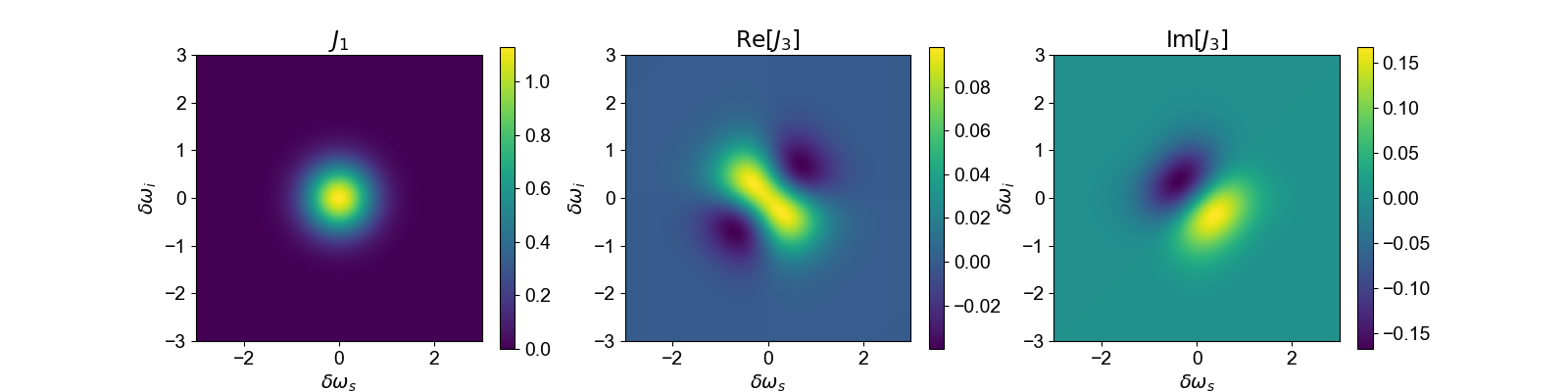
Figure S4: First-order joint spectral mode $J_{1}(\omega_{s},\omega_{i})$ [Eq. (S44)] and the next leading order mode $J_{3}(\omega_{s},\omega_{i})$ [Eq. (S47)] using parameters $\eta_{a}=-\eta_{b}=\tau=1$.

.4 Signal and idler group delay

In this section, we derive an analytic expression for the group delay between the signal and idler photons using the joint spectral amplitude obtained in Sec. .3. Up to third order in the Magnus expansion, the joint spectral amplitude is given by

$$J(\omega_{s},\omega_{i})=\varepsilon J_{1}(\omega_{s},\omega_{i})+\varepsilon^{3}J_{3}(\omega_{s},\omega_{i})$$ (S48)

where $J_{1}(\omega_{s},\omega_{i})$ is given by Eq. (S44) and $J_{3}(\omega_{s},\omega_{i})=L_{3}(\omega_{s},\omega_{i})-iK_{3}(\omega_{s},\omega_{i})$ is given by Eq. (S47). To obtain an expression for the group delay, we first compute the joint spectral phase which is given by:

$$\arg{[J(\omega_{s},\omega_{i})]}=\arctan{\left(\frac{\mathrm{Im}[J(\omega_{s},\omega_{i})]}{\mathrm{Re}[J(\omega_{s},\omega_{i})]}\right)}=\arctan{\left(\frac{-\varepsilon^{3}K_{3}(\omega_{s},\omega_{i})}{\varepsilon J_{1}(\omega_{s},\omega_{i})+\varepsilon^{3}L_{3}(\omega_{s},\omega_{i})}\right)}.$$ (S49)

Note that $f_{0}(\delta\omega_{s,i})=f_{0}(-\delta\omega_{s,i})$ and $f_{1}(-\delta\omega_{s,i})=-f_{1}(\delta\omega_{s,i})$. As a result, $\mathrm{Re}[J(\omega_{s},\omega_{i})]=\mathrm{Re}[J(\omega_{i},\omega_{s})]$ and $\mathrm{Im}[J(\omega_{s},\omega_{i})]=-\mathrm{Im}[J(\omega_{i},\omega_{s})]$, i.e. the real part of $J(\omega_{s},\omega_{i})$ is a symmetric function whereas its imaginary part is an anti-symmetric function, which can also be seen in Fig. S4. Along the anti-diagonal axis $\delta\omega_{s}=-\delta\omega_{i}\equiv\delta\omega$, we find

$$\begin{split}\arg{[J(\omega_{s},\omega_{i})]}&=\arctan{\left(\frac{\frac{\varepsilon^{2}}{2\sqrt{3}}f_{0}(\delta\omega)f_{1}(\delta\omega)}{f^{2}_{0}(\delta\omega)+\frac{\varepsilon^{2}}{12}\left\{f^{2}_{0}(\delta\omega)+f^{2}_{1}(\delta\omega)\right\}}\right)}\\ &=\arctan{\left(\frac{\varepsilon^{2}\mathrm{erfi}(\sqrt{4/3}\tau\delta\omega)}{2+\frac{\varepsilon^{2}}{6}(1+\mathrm{erfi}^{2}(\sqrt{4/3}\tau\delta\omega))}\right)}.\end{split}$$ (S50)

Using a Taylor expansion, we can approximate that $\mathrm{erfi}(x)\approx 2x/\sqrt{\pi}$ and $\mathrm{arctan}(x)\approx x$ for $x\ll 1$ and arrive at

$$\begin{split}\arg{[J(\omega_{s},\omega_{i})]}&\approx\left(\frac{24\varepsilon^{2}\tau}{\sqrt{3\pi}(12+\varepsilon^{2})}\right)\delta\omega+\mathcal{O}(\delta\omega^{2})\\ &=\frac{\beta}{2}\left(\delta\omega_{s}-\delta\omega_{i}\right)\end{split}$$ (S51)

where we defined $\beta\equiv\left(\frac{24\varepsilon^{2}\tau}{\sqrt{3\pi}(12+\varepsilon^{2})}\right)$.

In our derivation of the joint spectral amplitude in Sec. .3, we worked in the interaction picture and thus have not accounted for the phase that the fields accumulate through linear propagation inside the crystal. As shown in Ref. [58], this phase can be recovered by transforming the field operators according to:

$$\hat{a}^{\dagger}_{\mu}\rightarrow\hat{a}^{\dagger}_{\mu}e^{i\Delta k_{\mu}(\omega_{\mu})z_{0}}$$ (S52)

where $z_{0}=-L/2$ is the start of the crystal [see Eqn. (S36)] and $\Delta k_{\mu}(\omega_{\mu})=(v_{\mu}^{-1}-v_{p}^{-1})\delta\omega_{\mu}$. This results in an additional phase factor in the joint spectral amplitude:

$$J(\omega_{s},\omega_{s})\rightarrow J(\omega_{s},\omega_{s})\exp{[-i\Delta k_{s}(\omega_{s})L/2-i\Delta k_{i}(\omega_{i})L/2]}.$$ (S53)

Expanding this phase factor, we find

$$\begin{split}\exp{[-i\Delta k_{s}(\omega_{s})L/2-i\Delta k_{i}(\omega_{i})L/2]}&=\exp{\left[-i\frac{L}{2}\left(v_{s}^{-1}-v_{p}^{-1}\right)\delta\omega_{s}-i\frac{L}{2}\left(v_{i}^{-1}-v_{p}^{-1}\right)\delta\omega_{i}\right]}\\ &=\exp{\left[-i\frac{L}{4}\left(v_{s}^{-1}-v_{i}^{-1}\right)\left(\delta\omega_{s}-\delta\omega_{i}\right)\right]}\end{split}$$ (S54)

where, in the second line, we used the conditions (i) $v_{s}^{-1}-v_{p}^{-1}=-(v_{i}^{-1}-v_{p}^{-1})$ and (ii) $v_{s}^{-1}-v_{p}^{-1}=\frac{1}{2}\left(v_{s}^{-1}-v_{i}^{-1}\right)$ due to symmetric group velocity matching. Thus, Eq. (S51) becomes modified to:

$$\arg{[J(\omega_{s},\omega_{i})]}=\frac{(\beta-\beta_{0})}{2}(\delta\omega_{s}-\delta\omega_{i})$$ (S55)

where $\beta_{0}=\frac{L}{2}\left(v_{s}^{-1}-v_{i}^{-1}\right)$ is a gain-independent group delay between signal and idler photons corresponding to these being generated half-way through the crystal [5]. By the Fourier shift theorem, the linear spectral phase gradient in Eq. (S55) results in a group delay of $(\beta_{0}-\beta)/2$ for the signal photon and $-(\beta_{0}-\beta)/2$ the idler photon. Hence, the total delay between the two photons is $T=\beta_{0}-\beta$.

.5 Spectrally-resolved coincidences

In Eq. (7), we derived the spectrally-resolved coincidence probability $\mathrm{pr}(\omega_{1},\omega_{2})$ by projecting the SPDC light after the beam splitter $\ket{\tilde{\Psi}}_{cd}$ onto pure single photons, i.e. $\mathrm{pr}(\omega_{1},\omega_{2})=\left|\bra{\omega_{1}}_{c}\bra{\omega_{2}}_{d}\ket{\tilde{\Psi}}_{cd}\right|^{2}$ where $\ket{\omega_{1}}_{c}\ket{\omega_{2}}_{d}=\hat{c}^{\dagger}(\omega_{1})\hat{d}^{\dagger}(\omega_{2})\ket{0}_{c}\ket{0}_{d}$. In a low-gain regime where $\braket{n}\ll 1$, this projection measurement can be achieved using threshold (i.e. “click”) detectors since the probability to measure a coincidence is dominated by the single photon pair term of $\ket{\tilde{\Psi}}_{cd}$. Optical losses merely reduce the rate of measuring these coincidences. However, this approximation no longer holds in a high-gain regime because larger photon-number terms can also lead to a click event. A complete description of the threshold detector statistics would require computing the spectrally-resolved Torontonians of the multimode lossy squeezed state [83]. Below, we develop a simpler model which assumes that: (i) the squeezing operator acts in a single spatiotemporal mode, and (ii) the losses are sufficiently high such that the attenuated state only contains vacuum, one, or two-photon components. This simpler model captures the relevant features of our observations, namely that the spectrally-resolved coincidences pattern contains an interference term which depends on the group delay and the marginals of the joint spectral amplitude.

Using assumption (i), the joint spectral amplitude of the signal and idler modes is given by

$$J(\omega_{s},\omega_{i})=j_{s}(\omega_{s})\times j_{i}(\omega_{i})\times e^{-i\frac{T}{2}(\omega_{s}-\omega_{i})}$$ (S56)

where $j_{s}(\omega)=\int d\omega_{i}|J(\omega,\omega_{i})|$ and $j_{i}(\omega)=\int d\omega_{s}|J(\omega_{s},\omega)|$ are their respective marginal spectral amplitude, $T$ is the group delay between the photon pairs. Defining the following operators,

$$\begin{split}\hat{A}\equiv\int d\omega j_{s}(\omega)e^{-i\frac{T}{2}\omega}\hat{a}(\omega)\\ \hat{B}\equiv\int d\omega j_{i}(\omega)e^{i\frac{T}{2}\omega}\hat{b}(\omega)\end{split}$$ (S57)

we can re-write the SPDC output state as

$$\ket{\Psi}_{ab}=\exp{[\epsilon\hat{A}^{\dagger}\hat{B}^{\dagger}-\mathrm{h.c.}]}\ket{0}$$ (S58)

where the average photon number in each output mode is $\braket{n}=\sinh^{2}{(\epsilon)}$. We then attenuate $\ket{\Psi}_{ab}$ down to the single-photon level in order to measure spectrally-resolved intensity correlations with threshold detectors. The attenuation is modeled by placing a beam splitter with transmission $\eta$ in both the signal and idler modes then tracing over the reflected mode. By working in a Gaussian formalism, one can show that the output state is given by [84]:

$$\hat{\rho}_{ab}=\mathrm{exp}[\epsilon^{\prime}\hat{A}^{\dagger}\hat{B}^{\dagger}-\mathrm{h.c.}]\left(\hat{\rho}_{a}^{\mathrm{th}}\otimes\hat{\rho}_{b}^{\mathrm{th}}\right)\mathrm{exp}[\epsilon^{\prime}\hat{A}\hat{B}-\mathrm{h.c.}].$$ (S59)

Eq. (S59) describes a “squashed state”, which is obtained by applying a two-mode squeezing operator with gain $\epsilon^{\prime}$ given by $\tanh{(2\epsilon^{\prime})}=\left(2\eta\sinh{(\epsilon)}\cosh{(\epsilon)}\right)/\left(2\sinh^{2}{(\epsilon)}\eta+1\right)$ onto thermal states $\hat{\rho}_{a,b}^{\mathrm{th}}$ with mean occupation $\bar{n}=[1+2\eta\braket{n}-4\eta^{2}\braket{n}^{2}]^{1/2}-1$. In the limit where $\eta\rightarrow 0$, we find that $\epsilon^{\prime}\sim 0$ and $\bar{n}\sim\eta\braket{n}$, and thus the attenuated output state is two uncorrelated thermal states [85, 86]:

$$\hat{\rho}_{ab}=\hat{\rho}_{a}^{\mathrm{th}}\otimes\hat{\rho}_{b}^{\mathrm{th}}=\left(\sum_{n=0}^{\infty}\frac{\lambda^{n}}{n!}(\hat{A}^{\dagger})^{n}\ket{0}_{a}\bra{0}_{a}\hat{A}^{n}\right)\otimes\left(\sum_{j=0}^{\infty}\frac{\lambda^{j}}{j!}(\hat{B}^{\dagger})^{j}\ket{0}_{b}\bra{0}_{b}\hat{B}^{j}\right)$$ (S60)

where $\lambda=\eta\braket{n}/(1+\eta\braket{n})$. We then combine the two thermal states onto a beam splitter which performs the unitary transformation $\hat{U}_{ab}^{\dagger}\hat{a}\hat{U}_{ab}=(\hat{a}+\hat{b})/\sqrt{2}$ and $\hat{U}_{ab}^{\dagger}\hat{b}\hat{U}_{ab}=(\hat{a}-\hat{b})/\sqrt{2}$. If we measure spectrally-resolved coincidences at the output of the beam splitter, we find:

$$\begin{split}\mathrm{pr}(\omega_{1},\omega_{2})&=\bra{0}_{a}\bra{0}_{b}\hat{a}(\omega_{1})\hat{b}(\omega_{2})U_{ab}\hat{\rho}_{ab}U_{ab}^{\dagger}\hat{a}^{\dagger}(\omega_{1})\hat{b}^{\dagger}(\omega_{2})\ket{0}_{a}\ket{0}_{b}\\ &=\frac{1}{4}\bigg{(}\bra{\omega_{1}}_{a}\bra{\omega_{2}}_{a}\hat{\rho}_{ab}\ket{\omega_{1}}_{a}\ket{\omega_{2}}_{a}+\bra{\omega_{1}}_{a}\bra{\omega_{2}}_{b}\hat{\rho}_{ab}\ket{\omega_{1}}_{a}\ket{\omega_{2}}_{b}\\ &\qquad+\bra{\omega_{2}}_{a}\bra{\omega_{1}}_{b}\hat{\rho}_{ab}\ket{\omega_{2}}_{a}\ket{\omega_{1}}_{b}+\bra{\omega_{1}}_{b}\bra{\omega_{2}}_{b}\hat{\rho}_{ab}\ket{\omega_{1}}_{b}\ket{\omega_{2}}_{b}\\ &\qquad-\bra{\omega_{1}}_{a}\bra{\omega_{2}}_{b}\hat{\rho}_{ab}\ket{\omega_{2}}_{a}\ket{\omega_{1}}_{b}-\bra{\omega_{2}}_{a}\bra{\omega_{1}}_{b}\hat{\rho}_{ab}\ket{\omega_{1}}_{a}\ket{\omega_{2}}_{b}\bigg{)}\\ &=\frac{1}{4}\bigg{(}2\lambda^{2}j_{a}^{2}(\omega_{1})j_{a}^{2}(\omega_{2})+\lambda^{2}j_{a}^{2}(\omega_{1})j_{b}^{2}(\omega_{2})\\ &\qquad+\lambda^{2}j_{a}^{2}(\omega_{2})j_{b}^{2}(\omega_{1})+2\lambda^{2}j_{b}^{2}(\omega_{1})j_{b}^{2}(\omega_{2}))\\ &\qquad-\lambda^{2}j_{a}(\omega_{1})j_{a}(\omega_{2})j_{b}(\omega_{1})j_{b}(\omega_{2})e^{-i\frac{T}{2}(\omega_{1}-\omega_{2})}\\ &\qquad-\lambda^{2}j_{a}(\omega_{1})j_{a}(\omega_{2})j_{b}(\omega_{1})j_{b}(\omega_{2})e^{-i\frac{T}{2}(\omega_{2}-\omega_{1})}\bigg{)}\\ \end{split}$$ (S61)

where we used the fact that

$$\begin{split}\bra{\omega_{1}}_{a}\bra{\omega_{2}}_{a}(\hat{A}^{\dagger})^{2}\ket{0}_{a}&=\bra{0}_{a}\hat{a}(\omega_{1})\hat{a}(\omega_{2})\iint d\omega d\omega^{\prime}j_{a}(\omega)j_{a}(\omega^{\prime})e^{i\frac{T}{2}(\omega+\omega^{\prime})}\hat{a}^{\dagger}(\omega)\hat{a}^{\dagger}(\omega^{\prime})\ket{0}_{a}\\ &=2j_{a}(\omega_{1})j_{a}(\omega_{2})e^{i\frac{T}{2}(\omega_{1}+\omega_{2})}.\end{split}$$ (S62)

Eq. (S61) describes an interference pattern with a fringe along the $\omega_{1}=-\omega_{2}$ axis. The factors of $2$ in the first two terms of Eq. (S61) reflect the thermal statistics of the pulses in each spatial mode: it is two times more likely to find two photons in one of the pulses than one photon in each pulse. If the signal and idler spectral amplitudes are indistinguishable, i.e. $j_{a}(\omega)=j_{b}(\omega)\equiv j(\omega)$, the equation can be simplified to:

$$\mathrm{pr}(\omega_{1},\omega_{2})\propto[j(\omega_{1})j(\omega_{2})]^{2}\left[3-\cos\left(\tfrac{T}{2}[\omega_{1}-\omega_{2}]\right)\right].$$ (S63)

Effects such as multiple temporal-spectral modes, larger photon-number terms, and dark counts can all further reduce the interference visibility $\mathcal{V}$, leading to Eq. (8) in the main text.

.6 Further details on experimental results

Our experiment employs a two-element superconducting nanowire detector. We can measure up to two clicks in both the “early” bin (transmitted mode of PBS) and the “late” bin (reflected mode of PBS). The histograms $N(\omega_{1},\omega_{2})$ are obtained by binning timetags of events where at least one photon is detected in both the “early” and “late” bins. In Fig. S5, we plot all measured $N(\omega_{1},\omega_{2})$. The center of the distributions are shifted towards higher frequencies with increasing $\varepsilon$. This is due to a pile-up effect whereby photons that arrive at the detector earlier (i.e. with higher frequencies) are more likely to be detected than photons which arrive at the detector later due to the detector deadtime ($\sim 100~{}$ns). Although this effect can be reduced by increasing the attenuation of the down-converted beams, it does not hinder our ability to resolve the fringe frequency and therefore we keep the attenuation constant to reduce the number of parameters in the model. All parameters used in the NeedALight model are given in Table 1.

To determine the $\chi^{(3)}$ nonlinear coefficients $\gamma_{s,i,p}$, we monitor the pump spectrum after the ppKTP crystal. The self-phase modulation (SPM) coefficient, $\gamma_{p}$ is obtained by fitting a SPM model implemented in NeedALight [Fig S8]. The cross-phase modulation (XPM) coefficients are then given by $\gamma_{i}=2\gamma_{p}$ and $\gamma_{s}=2\gamma_{p}/3$ [87]. These nonlinear coefficients $\gamma_{\mu}$ can be related to the coupling constants $\zeta_{\mu}$ through the equation $\gamma_{\mu}=\zeta_{\mu}/v_{p}v_{\mu}\hbar\bar{\omega}_{\mu}$ [58]. In Fig. S6, we compare our experimental data to the NeedALight model with and without including $\chi^{(3)}$ effects. Due to XPM, there is a small additional group delay between the signal and idler photon pulses. However, most of the observed delay can be attributed to high-gain $\chi^{(2)}$ interactions.

To determine the parametric gain $\varepsilon$, we first rotate the HWP such that the signal and idler modes are separated at the PBS. Then, we record the click statistics for five minutes at each pump power. Using these statistics, we fit a model that uses Strawberryfields [88] to simulate a two-mode squeezed vacuum state of squeezing $\varepsilon$ being detected by four threshold detectors of efficiency $\eta$. The efficiency $\eta\sim 7\%$ was determined from a Klyshko measurement at low gain. The resulting parametric gains are shown in Fig. S7. Although our Strawberryfields model neglects the slight spectrally multimode nature of the down-converted light, this method of determining $\varepsilon$ provides a sufficiently good estimate to obtain agreement with NeedALight for the group delay [Fig. 3(d)].

Parameter	Value	Method
Pump
Spectral amplitude bandwidth $\sigma$	3.22(5) nm	Spectrometer
Pulse amplitude duration $\tau$	132(3) fs	Frequency-resolved optical gating (FROG)
Center wavelength	779.2 nm	Spectrometer
Down-conversion source
Crystal length $L$	$2$ mm	Manufacturer (Raicol)
Signal efficiency $\eta_{s}$	7(1) %	Klyshko measurement at low gain
Idler efficiency $\eta_{i}$	7(1) %	Klyshko measurement at low gain
Parametric gain $\varepsilon$	0 to $\sim$ 3	Fitting click statistics using $\eta_{s,i}$ [89]
Pump SPM coefficient $\gamma_{p}$	$0.07(2)~{}\mathrm{W}^{-1}\mathrm{m}^{-1}$	Fitting pump spectrum after crystal [Fig. S8]
Signal XPM coefficient $\gamma_{s}$	$0.05(1)~{}\mathrm{W}^{-1}\mathrm{m}^{-1}$	$\gamma_{s}=2\gamma_{p}/3$
Idler XPM coefficient $\gamma_{i}$	$0.14(4)~{}\mathrm{W}^{-1}\mathrm{m}^{-1}$	$\gamma_{i}=2\gamma_{p}$
Pump (H-pol) group index $\bar{n}_{p}$	1.8092	Ref. [69]
Signal (V-pol) group index $\bar{n}_{s}$	1.8514	Ref. [69]
Idler (H-pol) group index $\bar{n}_{i}$	1.7538	Ref. [69]

Table 1: A list of the parameters used in NeedALight. Note that the bandwidths specify one standard deviation of the amplitude functions rather than the intensity. The nonlinear coefficients $\gamma_{\mu}$ can be related to the coupling constants $\zeta_{\mu}$ through the equation $\gamma_{\mu}=\zeta_{\mu}/v_{p}v_{\mu}\hbar\bar{\omega}_{\mu}$ [58].

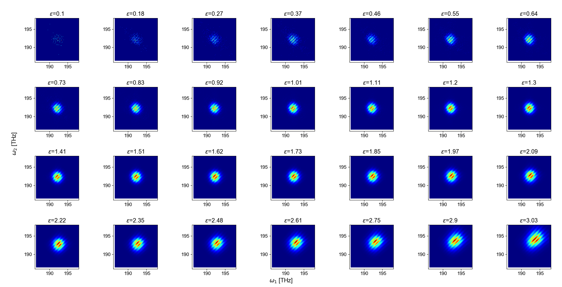
Figure S5: Complete dateset for the spectrally-resolved coincidences $N(\omega_{1},\omega_{2})$.

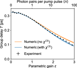
Figure S6: Comparison of the numeric NeedALight model with and without including $\chi^{(3)}$ effects (i.e. self-phase and cross-phase modulation). Most of the observed group delay can be attributed to a high-gain $\chi^{(2)}$ effect.

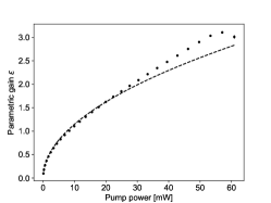
Figure S7: The experimental parametric gain $\varepsilon$ values [black dots]. In the low gain regime, $\varepsilon\propto\sqrt{P}$ [dashed line] where $P$ is the pump power [49].

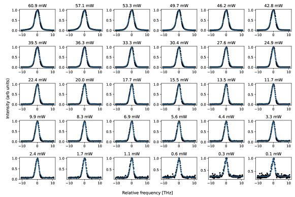
Figure S8: Measured pump spectra after the ppKTP crystal. Blue line is a fit obtained using NeedALight. The spectra broaden with increasing power due to self-phase modulation.