Improved Downlink Channel Estimation in Time-Varying FDD Massive MIMO Systems

Abstract

In this work, we address the challenge of accurately obtaining channel state information at the transmitter (CSIT) for frequency division duplexing (FDD) multiple input multiple output systems. Although CSIT is vital for maximizing spatial multiplexing gains, traditional CSIT estimation methods often suffer from impracticality due to the substantial training and feedback overhead they require. To address this challenge, we leverage two sources of prior information simultaneously: the presence of limited local scatterers at the base station (BS) and the time-varying characteristics of the channel. The former results in a redundant angular sparsity of users’ channels exceeding the spatial dimension (i.e., the number of BS antennas), while the latter provides a prior non-uniform distribution in the angular domain. We propose a weighted optimization framework that simultaneously reflects both of these features. The optimal weights are then obtained by minimizing the expected recovery error of the optimization problem. This establishes an analytical closed-form relationship between the optimal weights and the angular domain characteristics. Numerical experiments verify the effectiveness of our proposed approach in reducing the recovery error and consequently resulting in decreased training and feedback overhead.

I Introduction

Massive multiple input multiple output (MIMO) technology holds significant promise for enhancing wireless communication capacity by capitalizing on increased degrees of freedom [1]. Researchers have expressed considerable interest in exploring its applications in next-generation wireless systems [2]. However, to fully leverage the spatial multiplexing and array gains of (massive) MIMO, precise channel state information at the Transmitter (CSIT) is indispensable [3, 4]. While time division duplexing (TDD) MIMO systems can utilize channel reciprocity for CSIT acquisition using uplink pilots, acquiring CSIT for frequency division duplexing (FDD) systems presents challenges due to significant overheads [5, 6].

In FDD systems – shown in Figure 1 – CSIT at the base station (BS) is typically obtained by transmitting downlink pilot symbols and estimating the downlink channel state information locally at the user, which is then fed back to the BS via uplink signaling channels [7]. Conventional methods, such as least squares (LS) and minimum mean square error (MMSE), for downlink CSI estimation require a large number of orthogonal pilot symbols, which is linearly proportional to the number of BS antennas [7]. This overhead significantly increases in massive MIMO systems, rendering conventional methods in FDD systems impractical [6].

To tackle this challenge effectively, it is essential to leverage prior channel information in massive MIMO systems. The inherent angular sparsity observed in the user channel matrices within these systems [8] offers valuable insights that can be exploited through compressed sensing (CS) techniques [9, 10, 11]. However, existing CS-based methods in massive MIMO often assume an equal amount of information in both the angular and the spatial domains, or, alternatively, they assume the number of angular bins to be equal to the number of BS antennas, while indeed the angular domain is a much larger space than the spatial domain. This redundancy in angular domain can be effectively utilized through $\ell_{1}$ analysis optimization [9] rather than the conventional $\ell_{1}$ optimization used for capturing sparsity [12, 13, 14]. By employing a larger number of angular bins than BS antennas, we can achieve better accuracy in sparse representation within the angular domain.

Additionally, the dynamic nature of time-varying wireless channels provides a non-uniform prior distribution in the angular domain, which can be utilized in advance. For instance, due to the limited range of each user on the ground compared to a BS located at a higher elevation, only a fraction of the angular domain is active during user movement, while the rest remains inactive, leading to a non-uniform distribution in the angular domain. In this work, we propose a weighted $\ell_{1}$ analysis optimization that simultaneously captures both the redundant angular sparsity and the non-uniform angular prior distribution. We determine the optimal weights by minimizing the expected recovery error of the proposed optimization problem, which is equivalent to minimizing the statistical dimension [10, 11] of a certain cone. Note that the statistical dimension provides the minimum number of pilot symbols that the proposed optimization problem requires for exact channel estimation. Numerical experiments demonstrate the effectiveness of our approach in reducing the recovery error, thereby implying a reduction in the training and feedback overhead.

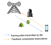
Figure 1: The BS transmits compressive training pilot to users. Each user locally obtains the compressive measurement and feeds back to the BS. The BS then recovers the CSIT based on the collected compressive measurements.

Notation. $\mathds{P}$ and $\mathds{E}$ denote the probability and expectation operators, respectively. matrices and vectors are shown by bold upright letters. ${\rm cone}(S)$ denotes the conic hull of a set. $\partial f(\mathbf{x})$ denotes the sub-differential of the function $f$ at point $\mathbf{x}\in\mathbb{C}^{n}$. ${\rm erf}$ denotes the error function. $\mathbf{g}\in\mathbb{C}^{n}$ is a vector with i.i.d. elements and standard normal distribution. The sign of a vector is defined as ${\rm sgn}(\mathbf{x})\mathbin{\setstackgap{S}{0pt}\stackMath\Shortstack{\smalltriangleup\\ =}}\tfrac{\mathbf{x}}{\|\mathbf{x}\|_{2}}$. $a\wedge b$ stands for the minimum of $a$ and $b$. $\mathbf{v}\in\mathbb{R}_{++}^{n}$ means that $v(i)>0\forall i$. The infinity norm is defined as $\|\mathbf{z}\|_{\infty}=\max_{i}|z(i)|$. $x(l)$ is the $l$-th element of $\mathbf{x}\in\mathbb{C}^{n}$. The null space of a matrix is denoted by ${\rm null}(\cdot)$.

II System Model

We consider a massive MIMO FDD system shown in Figure 1 with single-antenna users and assume the BS is equipped with $n$ antennas distributed as uniform linear array. For the downlink channel estimation in FDD system, the BS transmits pilots to users. The users receive the pilots and feeds the received signal back to the BS directly in an ideal channel as in e.g., [12, 15]. The received downlink signal can be written as

$$\mathbf{y}=\mathbf{A}\mathbf{h}+\mathbf{e}\in\mathbb{C}^{m\times 1},$$ (1)

where $\mathbf{h}\in\mathbb{C}^{n\times 1}$ is the downlink spatial channel, $\mathbf{A}\in\mathbb{C}^{m\times n}$ is the downlink pilot matrix, $m\ll n$ is the pilot length and $\mathbf{e}\in\mathbb{C}^{m\times 1}$ is the additive measurement noise with $\|\mathbf{e}\|_{2}\leq\eta$. Experimental studies have shown that the channel exhibits sparsity in the angular domain [8]. However, the dimension of the angular domain significantly exceeds that of the spatial domain, denoted as $n$. This suggests that upon applying an analysis operator $\bm{\Omega}\mathbin{\setstackgap{S}{0pt}\stackMath\Shortstack{\smalltriangleup\\ =}}[\bm{\omega_{1}},...,\bm{\omega}_{p}]^{T}\in\mathbb{C}^{p\times n},p\gg n$ to the spatial domain, we get to the angular sparse domain. Here, $\bm{\omega}_{i}=[1,...,{\rm e}^{-2\pi(n-1)d\leavevmode\nobreak\ \sin(\theta_{i})}]^{\rm T}\in\mathbb{C}^{n\times 1}$ is the steering vector for angular bin $\theta_{i}$ and $d$ is the BS antenna spacing. Mathematically, we may express the downlink channel in the angular domain as

$$\mathbf{h}_{\rm a}=\bm{\Omega}\mathbf{h}\in\mathbb{C}^{p\times 1},$$ (2)

where the number of angular bins $p$ is much larger than the number $n$ of BS antennas. Here, $\mathbf{h}_{\rm a}\in\mathbb{C}^{p}$ is a sparse vector with analysis support $\mathcal{S}$ which represent angular bins that $h_{\rm a}(i)\neq 0,i=1,...,p$. The analysis Fourier operator $\bm{\Omega}$ is no longer orthonormal; however, it remains orthogonal. This implies that $\bm{\Omega}^{\rm H}\bm{\Omega}=\mathbf{I}_{n}$, but $\bm{\Omega}\bm{\Omega}^{\rm H}\neq\mathbf{I}_{p}$. The sparsity in the redundant angular domain is called analysis sparsity. To promote angular analysis sparsity, one can solve the following optimization problem [9]:

$$\mathsf{P}_{\bm{\Omega}}:\leavevmode\nobreak\ \leavevmode\nobreak\ \min_{\mathbf{z}\in\mathbb{C}^{n}}\|\bm{\Omega z}\|_{1}\mathbin{\setstackgap{S}{0pt}\stackMath\Shortstack{\smalltriangleup{\\ }=}}\sum_{i=1}^{p}|(\bm{\Omega z})_{i}|\leavevmode\nobreak\ \leavevmode\nobreak\ {\rm s.t.}\leavevmode\nobreak\ \|\mathbf{y}_{m\times 1}-\mathbf{A}\mathbf{z}\|_{2}\leq\eta,$$ (3)

In practice, due to the time-varying nature of the channel, there is a prior distribution of ${h}_{\rm a}(k)$ for each angular bin $k=1,...,p$ which together with redundant angular sparsity can be exploited. This angular distribution is non-uniformly distributed among angular bins. To promote angular sparsity and non-uniform structure together, we propose to use the following weighted optimization problem:

$$\mathsf{P}_{\bm{\Omega},\mathbf{v}}:\leavevmode\nobreak\ \min_{\mathbf{z}\in\mathbb{C}^{n}}\|\bm{\Omega z}\|_{1,\mathbf{v}}\mathbin{\setstackgap{S}{0pt}\stackMath\Shortstack{\smalltriangleup{\\ }=}}\sum_{i=1}^{p}v_{i}|(\bm{\Omega z})_{i}|\leavevmode\nobreak\ {\rm s.t.}\|\mathbf{y}_{m\times 1}-\mathbf{A}\mathbf{z}\|_{2}\leq\eta,$$ (4)

where the weights $\mathbf{v}=\{v_{1},\dots,v_{p}\}$ are some positive scalars served to penalize the angles that are less likely to be on the analysis support $\mathcal{S}$. In the next section, we provide an analytical way to determine the optimal weights in (4).

III Main result

In this section, we aim to find an upper-bound for the recovery error of problem $\mathsf{P}_{\bm{\Omega},\mathbf{v}}$ in (4). Before that we require to define the expected joint sign parameter between $h_{a}(i)$ and $h_{a}(j)$ in the angular domain as follows:

$$\sigma_{i,j}\mathbin{\setstackgap{S}{0pt}\stackMath\Shortstack{\smalltriangleup{\\ }=}}\mathds{E}[{\rm sgn}(h_{a}(i)){\rm sgn}(h_{a}(j))]=$$

$$\int\int{\rm sgn}(a){\rm sgn}(b)f_{h_{a}(i),h_{a}(j)}(a,b){\rm d}a{\rm d}b$$ (5)

where $f_{h_{a}(i),h_{a}(j)}(a,b)$ is the joint PDF of $h_{a}(i)$ and $h_{a}(j)$ for any $i,j=1,...,p$. The joint support distribution and the support distribution are also defined as $\beta_{i,j}\mathbin{\setstackgap{S}{0pt}\stackMath\Shortstack{\smalltriangleup\\ =}}\mathds{P}(i\in\mathcal{S},j\in\mathcal{S})$ and $\beta_{i}\mathbin{\setstackgap{S}{0pt}\stackMath\Shortstack{\smalltriangleup\\ =}}\mathds{P}(i\in\mathcal{S})$ for any $i,j=1,...,p$.

Theorem 1.

Let $\widehat{\mathbf{h}}\in\mathbb{C}^{n}$ be the solution of the optimization problem $\mathsf{P}_{\bm{\Omega},\mathbf{v}}$. Then, for any $\mathbf{v}\in\mathbb{R}_{+}^{p}$, the expected recovery error of $\mathsf{P}_{\bm{\Omega},\mathbf{v}}$ is bounded above by the following expression:

$$\mathds{E}_{\mathbf{h}}[\|\widehat{\mathbf{h}}-\mathbf{h}\|_{2}\leq\tfrac{2\eta}{\max\{\sqrt{m-1}-\sqrt{\mathds{E}_{\mathbf{h}}[\delta(\mathcal{D}(\|\bm{\Omega}\cdot\|_{1,\mathbf{v}},\mathbf{h}))]}-a,0\}}+c$$ (6)

with probability at least $1-{\rm e}^{-\tfrac{a^{2}}{2}}$ in which $c>0$ is a constant and $\mathds{E}_{\mathbf{h}}[\delta(\mathcal{D}(\|\bm{\Omega}\cdot\|_{1,\mathbf{v}},\mathbf{h}))]$ is the expected required sample complexity of $\mathsf{P}_{\bm{\Omega},\mathbf{v}}$ which is bounded from above as follows:

$$\mathds{E}_{\mathbf{h}}[\delta(\mathcal{D}(\|\bm{\Omega}\cdot\|_{1,\mathbf{v}},\mathbf{h}))]\leq$$

$$\inf_{t\geq 0}\Big{\{}n-\tfrac{\Big{(}\sum_{k=1}^{p}(1-\beta_{k})\|\bm{\omega}_{k}\|_{2}{\rm erf}(\tfrac{tv_{k}}{\sqrt{2}})\Big{)}^{2}}{F(t,\mathbf{v})}\Big{\}},$$ (7)

where

$$F(t,\mathbf{v})\mathbin{\setstackgap{S}{0pt}\stackMath\Shortstack{\smalltriangleup{\\ }=}}\sum_{i,j=1}^{p}(tv_{i})(tv_{j})\bm{\omega}_{i}^{\rm H}\bm{\omega}_{j}\sigma_{i,j}+\sum_{i,j=1}^{p}\tfrac{(\bm{\omega}_{i}^{\rm H}\bm{\omega}_{j})^{2}}{\|\bm{\omega}_{i}\|_{2}\|\bm{\omega}_{j}\|_{2}}$$

$$\bigg{[}{\rm erf}(\tfrac{tv_{\min}}{\sqrt{2}})-q(tv_{\max})(tv_{i})(tv_{j})\bigg{]}(1-\beta_{i}-\beta_{j}+\beta_{i,j})$$ (8)

and $q(t)\mathbin{\setstackgap{S}{0pt}\stackMath\Shortstack{\smalltriangleup\\ =}}\sqrt{\tfrac{2}{\pi}}\tfrac{{\rm e}^{-\tfrac{t^{2}}{2}}}{t}+{\rm erf}(\tfrac{t}{\sqrt{2}})-1$.

Proof. See Appendix Appendix A: Proof of Theorem 1.

Our proposed strategy to find optimal weights is to minimize the expected recovery error provided in (6). This leads to minimizing the upper-bound on the expected statistical dimension provided in (1). Specifically, the optimal weights can be found by solving the following optimization problem:

$$\mathbf{v}^{\star}=\mathop{\arg\min}_{\mathbf{v}>0}\inf_{t>0}\Big{\{}n-\tfrac{\Big{(}\sum_{k=1}^{p}(1-\beta_{k})\|\bm{\omega}_{k}\|_{2}{\rm erf}(\tfrac{tv_{k}}{\sqrt{2}})\Big{)}^{2}}{F(t,\mathbf{v})}\Big{\}}.$$ (9)

The observant reader might have noticed that altering the multiplicative scaling of $\mathbf{v}$ does not impact the optimization $\mathsf{P}_{\Omega,\mathbf{v}}$ in (4), given that the weight vector’s values hold significance relative to each other. Hence, we can redefine $t\mathbf{v}$ simply as $\mathbf{v}$, treating it as a single variable and transform the latter optimization into

$$\mathbf{v}^{\star}=\mathop{\arg\min}_{\mathbf{v}\in\mathbb{R}_{++}^{p}}\Big{\{}\tfrac{2\eta}{\max\{\sqrt{m-1}-\sqrt{\overline{\delta}(\mathbf{v})}-a,0\}}\Big{\}}$$ (10)

where

$$\overline{\delta}(\mathbf{v})\mathbin{\setstackgap{S}{0pt}\stackMath\Shortstack{\smalltriangleup{\\ }=}}n-\tfrac{\Big{(}\sum_{k=1}^{p}(1-\beta_{k})\|\bm{\omega}_{k}\|_{2}{\rm erf}(\tfrac{v_{k}}{\sqrt{2}})\Big{)}^{2}}{F_{1}(\mathbf{v})},$$ (11)

and

$$F_{1}(\mathbf{v})\mathbin{\setstackgap{S}{0pt}\stackMath\Shortstack{\smalltriangleup{\\ }=}}\sum_{k,k^{\prime}=1}^{p}\Bigg{[}v_{k}v_{k^{\prime}}\bm{\omega}_{k}^{\rm H}\bm{\omega}_{k^{\prime}}\sigma_{k,k^{\prime}}+\tfrac{(\bm{\omega}_{k}^{\rm H}\bm{\omega}_{k})^{2}}{\|\bm{\omega}_{k}\|_{2}\|\bm{\omega}_{k^{\prime}}\|_{2}}$$

$$\Big{(}{\rm erf}(\tfrac{v_{\rm min}}{\sqrt{2}})-q(v_{\rm max})v_{k}v_{k^{\prime}}\Big{)}(1-\beta_{k}-\beta_{k^{\prime}}+\beta_{k,k^{\prime}})\Bigg{]}.$$ (12)

IV Simulations

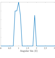
Figure 2: The prior support distribution $\beta_{k}\mathbin{\setstackgap{S}{0pt}\stackMath\Shortstack{\smalltriangleup\\ =}}\mathds{P}(k\in\mathcal{S}),k=1,...,p$ for a user considered in Section IV.

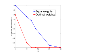
Figure 3: This figure shows the expected recovery error versus the number of pilot symbols. The blue lines shows the recovery performance of $\mathsf{P}_{\bm{\Omega}}$ with constant weights while the red line shows the performance of our proposed optimal weights provided in (10).

In this section, we examine a numerical experiment to evaluate the performance of our method. The support $\mathcal{S}$ is randomly selected from the subset $\{1,...,p\}$ with known distribution $\beta_{k},k=1,...,p$ shown in Figure 2 and the spatial channel is generated as $\mathbf{h}={\rm null}(\bm{\Omega}_{\overline{\mathcal{S}}})\mathbf{c}$ where $\mathbf{c}$ is a random vector uniformly distributed on the uniform sphere and $\overline{\mathcal{S}}$ is the complement of $\mathcal{S}$ in the angular domain. This ensures that $\mathbf{h}_{\rm a}$ has an analysis support $\mathcal{S}$. We form the pilot matrix $\mathbf{A}_{m\times n}$ from an i.i.d. Gaussian distribution and perform the signal recovery using two methods: $\ell_{1}$ analysis, weighted $\ell_{1}$ analysis (Problem $\mathsf{P}_{\bm{\Omega},\mathbf{v}}$) with the optimal weights which are provided in (10). The proposed near-optimal weights are obtained using support distribution $\{\beta_{k}\}_{k=1}^{p}$ and PDF of the channel in the angular domain i.e. $\{f_{h_{a}(k)}(\cdot)\}_{k=1}^{p}$ as prior information. Figure 3 shows the expected error defined by $\mathds{E}_{\mathbf{h},\mathbf{A}}\|\mathbf{h}-\widehat{\mathbf{h}}\|_{2}$ where $\widehat{\mathbf{h}}$ is the obtained estimate by solving $\mathsf{P}_{\bm{\Omega},\mathbf{v}}$. The latter expectation is calculated using $100$ independent Monte Carlo simulations over different $\mathbf{A}$ and $\mathbf{h}$. As shown in Figure 3, our proposed optimal weights provides a superior performance than the heuristic and constant weights in recovering the ground-truth channel from measurements $\mathbf{y}\in\mathbb{C}^{m}$.

V Conclusion

In this paper, we designed a new approach for downlink channel estimation in FDD massive MIMO systems in order to reduce the training and feedback overhead. Specifically, we proposed a weighted optimization problem for channel estimation that simultaneously promote redundant angular sparsity and non-uniform angular distribution. We obtained a close-form expression for the expected recovery error of the proposed optimization problem dependent on the weights and the channel angular characteristics. We then found the optimal weights by minimizing this expression. Numerical results showed how the angular sparsity and non-uniform angular distribution contributes to enhancing the CSIT estimation quality in massive MIMO systems.

Appendix A: Proof of Theorem 1

The recovery error in the problem $\mathsf{P}_{\bm{\Omega}}$ provided in (3) is explicitly connected to the statistical dimension of the descent cone produced by the objective function $\|\bm{\Omega}\cdot\|_{1,\mathbf{v}}$ at the ground-truth channel $\mathbf{h}$. This is stated in the following bound [16, Corrollary 3.5], [9]:

$$\|\widehat{\mathbf{h}}-\mathbf{h}\|_{2}\leq\tfrac{2\eta}{\max\{\sqrt{m-1}-\sqrt{\delta(\mathcal{D}(\|\bm{\Omega}\cdot\|_{1,\mathbf{v}},\mathbf{h}))}-a,0\}},$$ (13)

in which $\mathsf{P}_{\bm{\Omega},\mathbf{v}}$ fails with probability at most ${\rm e}^{-\tfrac{a^{2}}{2}}$. By taking the expectation from both sides of (13) and using the following Jensen’s gap inequality [17, Equation 2.1] and [18]:

$$\mathds{E}[\tfrac{1}{\max\{b-\sqrt{x},0\}}]<\tfrac{1}{\max\{b-\sqrt{\mathds{E}[x]},0\}}+c,$$ (14)

for any $x<b^{2}$ with $b>0$, it holds that

(15)

where $c>0$ is an upper-bound for the variance of the statistical dimension. Now, finding an upper-bound for the error requires to find an upper-bound for the expected statistical dimension. First, we begin with the definition of statistical dimension, i.e.

$$\delta(\mathcal{D}(\|\bm{\Omega}\cdot\|_{1,\mathbf{v}},\mathbf{h}))=\mathds{E}_{\mathbf{g}}{\rm dist}^{2}(\mathbf{g},{\rm cone}\partial\|\bm{\Omega}\cdot\|_{1}(\mathbf{h}))=$$

$$\mathds{E}_{\mathbf{g}}\inf_{t\geq 0}\inf_{\mathbf{z}\in\partial\|\bm{\Omega}\cdot\|_{1,\mathbf{v}}({\mathbf{h}})}\|\mathbf{g}-t\mathbf{z}\|_{2}^{2}.$$ (16)

By passing $\mathds{E}_{\mathbf{g}}$ through the first infimum, we reach an upper-bound as follows:

$$\mathds{E}_{\mathbf{g}}\inf_{t\geq 0}\inf_{\mathbf{z}\in\partial\|\bm{\Omega}\cdot\|_{1}({\mathbf{h}})}\|\mathbf{g}-t\mathbf{z}\|_{2}^{2}\leq\inf_{t\geq 0}\mathds{E}_{\mathbf{g}}\inf_{\mathbf{z}\in\partial\|\bm{\Omega}\cdot\|_{1,\mathbf{v}}({\mathbf{h}})}\|\mathbf{g}-t\mathbf{z}\|_{2}^{2}$$

$$=\inf_{t\geq 0}\mathds{E}_{\mathbf{g}}\inf_{\|\mathbf{z}\|_{\infty}\leq 1}\|\mathbf{g}-t\bm{\Omega}^{\rm H}\big{(}\mathbf{v}\odot{\rm sgn}(\bm{\Omega}\mathbf{h})\big{)}-t\bm{\Omega}^{\rm H}\big{(}\mathbf{v}\odot\mathbf{z}\big{)}\|_{2}^{2}$$

$$\mathbin{\setstackgap{S}{0pt}\stackMath\Shortstack{\smalltriangleup{\\ }=}}B_{u},$$ (17)

where in the last expression above, we used the chain rule of subdifferential (see [19, Chapter 23]) i.e. ${\partial\|\bm{\Omega}\cdot\|_{1,\mathbf{v}}(\mathbf{h})=\bm{\Omega}^{\rm H}\partial\|\cdot\|_{1,\mathbf{v}}(\bm{\Omega}\mathbf{h})}$ and the well-established relation for subdifferential of norm functions (see for example [20, Proposition 1]) i.e.

$$\partial\|\cdot\|_{1,\mathbf{v}}(\bm{\Omega}\mathbf{h})=\{\mathbf{v}\odot\big{(}{\rm sgn}(\bm{\Omega}\mathbf{h})+\mathbf{z}\big{)}:\leavevmode\nobreak\ \|\mathbf{z}\|_{\infty}\leq 1\}.$$ (18)

In [11], it is shown that $B_{u}$ is tight for different kinds of analysis operators. The expression $B_{u}$ does not seem to have a closed-form formula in general. Hence, we seek for an upper-bound of $B_{u}$. For this purpose, we substitute $\mathbf{z}$ with a special $\mathbf{z}^{\prime}=[z_{1}^{\prime},...,z_{p}^{\prime}]^{p}$ whose elements are defined as

$${z}_{i}^{\prime}\mathbin{\setstackgap{S}{0pt}\stackMath\Shortstack{\smalltriangleup{\\ }=}}\left\{\begin{array}[]{lr}0,&i\in\mathcal{S}\\ {\rm sgn}(\bm{\omega}_{i}^{\rm H}\mathbf{g})\big{(}\tfrac{(tv_{i})^{-1}\lambda|\bm{\omega}_{i}^{\rm H}\mathbf{g}|}{\|\bm{\omega}_{i}\|_{2}}\wedge 1\big{)},&i\in\overline{\mathcal{S}}\end{array}\right\},$$ (21)

where $\lambda>0$ is a flexible tuning parameter. With this choice of $\mathbf{z}$, we can proceed with (Appendix A: Proof of Theorem 1) as follows:

$$\mathds{E}_{\mathbf{g}}\|\mathbf{g}-t\bm{\Omega}^{\rm H}\big{(}\mathbf{v}\odot{\rm sgn}(\bm{\Omega}\mathbf{h})\big{)}-t\bm{\Omega}^{\rm H}\big{(}\mathbf{z}^{\prime}\odot\mathbf{v}\big{)}\|_{2}^{2}=$$

$$\mathds{E}_{\mathbf{g}}\|\mathbf{g}\|_{2}^{2}-2t\underbrace{\mathds{E}_{\mathbf{g}}\langle\mathbf{g},\bm{\Omega}^{\rm H}\big{(}\mathbf{v}\odot{\rm sgn}(\bm{\Omega}\mathbf{h})\big{)}\rangle}_{0}$$

$$-\underbrace{2t\mathds{E}_{\mathbf{g}}\langle\mathbf{g},\bm{\Omega}^{\rm H}\big{(}\mathbf{v}\odot\mathbf{z}^{\prime}\big{)}\rangle}_{\mathbin{\setstackgap{S}{0pt}\stackMath\Shortstack{\smalltriangleup{\\ }=}}V_{1}}+\underbrace{t^{2}\mathds{E}_{\mathbf{g}}\|\bm{\Omega}^{\rm H}\big{(}\mathbf{v}\odot\mathbf{z}^{\prime}\big{)}\|_{2}^{2}}_{\mathbin{\setstackgap{S}{0pt}\stackMath\Shortstack{\smalltriangleup{\\ }=}}V_{2}}+$$

$$\underbrace{t^{2}\|\bm{\Omega}^{\rm H}\big{(}\mathbf{v}\odot{\rm sgn}(\bm{\Omega x})\big{)}\|_{2}^{2}}_{\mathbin{\setstackgap{S}{0pt}\stackMath\Shortstack{\smalltriangleup{\\ }=}}V_{3}}=n-V_{1}+V_{2}+V_{3}.$$ (22)

Now, we calculate each term above one by one. First, consider

$$V_{1}=2t\mathds{E}_{\mathbf{g}}\langle\bm{\Omega}\mathbf{g},\mathbf{v}\odot\mathbf{z}^{\prime}\rangle=2t\sum_{i\in\overline{\mathcal{S}}}v_{i}\mathds{E}_{\bm{g}}\big{[}\bm{\omega}_{i}^{\rm H}\mathbf{g}z_{i}^{\prime}\big{]}$$

$$=2\sum_{i\in\overline{\mathcal{S}}}\mathds{E}_{\bm{g}}\bigg{[}|\bm{\omega}_{i}^{\rm H}\mathbf{g}|\big{(}\tfrac{\lambda|\bm{\omega}_{i}^{\rm H}\mathbf{g}|}{\|\bm{\omega}_{i}\|_{2}}\wedge tv_{i}\big{)}\bigg{]},$$ (23)

where we used the relation (21) in the last expression. Since $\bm{\omega}_{i}^{\rm H}\mathbf{g}\sim\mathcal{N}(\mathbf{0},\|\bm{\omega}_{i}\|_{2}^{2})$, it is straightforward to obtain the expectation inside the summation and verify that

$$V_{1}=2\sum_{i\in\overline{\mathcal{S}}}\|\bm{\omega}_{i}\|_{2}\mathds{E}_{\mathbf{g}}\big{[}|\mathbf{g}|(\lambda|\mathbf{g}|\wedge tv_{i})\big{]}.$$ (24)

We proceed by calculating

$$\mathds{E}_{\mathbf{g}}\big{[}|\mathbf{g}|(\lambda|\mathbf{g}|\wedge tv_{i})\big{]}=\int_{0}^{\tfrac{tv_{i}}{\lambda}}\lambda\sqrt{\tfrac{2}{\pi}}z^{2}{\rm e}^{-\tfrac{z^{2}}{2}}{\rm d}z+$$

$$\int_{\tfrac{tv_{i}}{\lambda}}^{\infty}\sqrt{\tfrac{2}{\pi}}tv_{i}z{\rm e}^{-\tfrac{z^{2}}{2}}{\rm d}z=\sqrt{\tfrac{2}{\pi}}tv_{i}{\rm e}^{-\tfrac{t^{2}v_{i}^{2}}{2\lambda^{2}}}-\sqrt{\tfrac{2}{\pi}}tv_{i}{\rm e}^{-\tfrac{t^{2}v_{i}^{2}}{2\lambda^{2}}}+$$

$$\lambda{\rm erf}(\tfrac{tv_{i}}{\sqrt{2}\lambda}),$$ (25)

which leads to

$$V_{1}=2\sum_{i\in\overline{\mathcal{S}}}\lambda\|\bm{\omega}_{i}\|_{2}{\rm erf}(\tfrac{tv_{i}}{\sqrt{2}\lambda}).$$ (26)

For $V_{2}$, we have

$$V_{2}=t^{2}\mathds{E}_{\mathbf{g}}\langle\mathbf{v}\odot\mathbf{z}^{\prime},\bm{\Omega}\bm{\Omega}^{\rm H}\big{(}\mathbf{v}\odot\mathbf{z}^{\prime}\big{)}\rangle=t^{2}\sum_{i,j\in\overline{\mathcal{S}}}v_{i}v_{j}\bm{\omega}_{i}^{\rm H}\bm{\omega}_{j}$$

$$\mathds{E}_{\mathbf{g}}[z_{i}^{\prime}z_{j}^{\prime}]=\sum_{i,j\in\overline{\mathcal{S}}}(tv_{i})(tv_{j})\bm{\omega}_{i}^{\rm H}\bm{\omega}_{j}\mathds{E}_{\mathbf{g}}\bigg{[}{\rm sgn}(\bm{\omega}_{i}^{\rm H}\mathbf{g}){\rm sgn}(\bm{\omega}_{j}^{\rm T}\mathbf{g})$$

$$\big{(}\tfrac{(tv_{i})^{-1}\lambda\bm{\omega}_{i}^{\rm H}\mathbf{g}}{\|\bm{\omega}_{i}\|_{2}}\wedge 1\big{)}\big{(}\tfrac{(tv_{j})^{-1}\lambda\bm{\omega}_{j}^{\rm T}\mathbf{g}}{\|\bm{\omega}_{j}\|_{2}}\wedge 1\big{)}\bigg{]}=\sum_{i,j\in\overline{\mathcal{S}}}\lambda^{2}\bm{\omega}_{i}^{\rm H}\bm{\omega}_{j}$$

$$\mathds{E}_{\mathbf{g}}\bigg{[}{\rm sgn}(\bm{\omega}_{i}^{\rm H}\mathbf{g}){\rm sgn}(\bm{\omega}_{j}^{\rm T}\mathbf{g})\big{(}\tfrac{|\bm{\omega}_{i}^{\rm H}\mathbf{g}|}{\|\bm{\omega}_{i}\|_{2}}\wedge\tfrac{tv_{i}}{\lambda}\big{)}\big{(}\tfrac{|\bm{\omega}_{j}^{\rm T}\mathbf{g}|}{\|\bm{\omega}_{j}\|_{2}}\wedge\tfrac{tv_{j}}{\lambda}\big{)}\bigg{]}$$ (27)

Deriving a closed-form formula for the final expression above appears to be challenging in general. In such cases, we resort to an upper bound provided in the following lemma, adapted from [21, Lemma 6.12].

Lemma 1.

[21, Lemma 6.12] Let $\mathbf{g}\sim\mathcal{N}(\mathbf{0},\mathbf{I}_{n})$. For any $\mathbf{z}_{1},\mathbf{z}_{2}\in\mathbb{S}^{n-1}$, $\alpha_{1},\alpha_{2}\geq 0$, and $\alpha_{\min}=\min\{\alpha_{1},\alpha_{2}\}$, $\alpha_{\max}=\max\{\alpha_{1},\alpha_{2}\}$, we have

$$\mathds{E}\bigg{[}{\rm sgn}(\mathbf{z}_{1}^{\rm T}\mathbf{g}){\rm sgn}(\mathbf{z}_{2}^{\rm T}\mathbf{g})\big{(}|\mathbf{z}_{1}^{\rm T}\mathbf{g}|\wedge\alpha_{1}\big{)}\big{(}|\mathbf{z}_{2}^{\rm T}\mathbf{g}|\wedge\alpha_{2}\big{)}\bigg{]}\leq$$

$$|\langle\mathbf{z}_{1},\mathbf{z}_{2}\rangle|\bigg{[}{\rm erf}(\tfrac{\alpha_{\min}}{\sqrt{2}})-q(\alpha_{\max})\alpha_{1}\alpha_{2}\bigg{]}.$$ (28)

By benefiting this lemma, we proceed (Appendix A: Proof of Theorem 1) as follows:

$$V_{2}\leq\lambda^{2}\sum_{i,j\in\overline{\mathcal{S}}}\tfrac{(\bm{\omega}_{i}^{\rm H}\bm{\omega}_{j})^{2}}{\|\bm{\omega}_{i}\|_{2}\|\bm{\omega}_{j}\|_{2}}\bigg{[}{\rm erf}(\tfrac{tv_{\min}}{\lambda\sqrt{2}})-q(\tfrac{tv_{\max}}{\lambda})\tfrac{(tv_{1})(tv_{2})}{\lambda^{2}}\bigg{]}.$$ (29)

Lastly, for $V_{3}$, it holds that

$$V_{3}=t^{2}\langle\mathbf{v}\odot{\rm sgn}(\bm{\Omega}\mathbf{h}),\bm{\Omega}\bm{\Omega}^{\rm H}\big{(}\mathbf{v}\odot{\rm sgn}(\bm{\Omega}\mathbf{h})\big{)}\rangle=$$

$$\sum_{i,j\in\mathcal{S}}(tv_{i})(tv_{j})\bm{\omega}_{i}^{\rm H}\bm{\omega}_{j}{\rm sgn}(\bm{\omega}_{i}^{\rm H}\mathbf{h}){\rm sgn}(\bm{\omega}_{j}^{\rm T}\mathbf{h}).$$ (30)

Combining (26), (29), (Appendix A: Proof of Theorem 1), and (Appendix A: Proof of Theorem 1), leads to the following upper-bound for $\delta(\mathcal{D}(\|\bm{\Omega}\cdot\|_{1,\mathbf{v}},\mathbf{h}))$.

$$\delta(\mathcal{D}(\|\bm{\Omega}\cdot\|_{1,\mathbf{v}},\mathbf{h}))\leq\inf_{t>0}\inf_{\lambda>0}\Bigg{\{}n+\sum_{i,j\in\mathcal{S}}(tv_{i})(tv_{j})\bm{\omega}_{i}^{\rm H}\bm{\omega}_{j}$$

$${\rm sgn}(\bm{\omega}_{i}^{\rm H}\mathbf{h}){\rm sgn}(\bm{\omega}_{j}^{\rm T}\mathbf{h})-2\sum_{i\in\overline{\mathcal{S}}}\lambda\|\bm{\omega}_{i}\|_{2}{\rm erf}(\tfrac{tv_{i}}{\sqrt{2}\lambda})+$$

$$\lambda^{2}\sum_{i,j\in\overline{\mathcal{S}}}\tfrac{(\bm{\omega}_{i}^{\rm H}\bm{\omega}_{j})^{2}}{\|\bm{\omega}_{i}\|_{2}\|\bm{\omega}_{j}\|_{2}}\bigg{[}{\rm erf}(\tfrac{tv_{\min}}{\lambda\sqrt{2}})-q(\tfrac{tv_{\max}}{\lambda})\tfrac{(tv_{1})(tv_{2})}{\lambda^{2}}\bigg{]}\Bigg{\}}.$$ (31)

By substituting $t$ by $\lambda t$, we have

$$\delta(\mathcal{D}(\|\bm{\Omega}\cdot\|_{1,\mathbf{v}},\mathbf{h}))\leq\inf_{t>0}\inf_{\lambda>0}\Bigg{\{}n+\lambda^{2}\sum_{i,j\in\mathcal{S}}(tv_{i})(tv_{j})\bm{\omega}_{i}^{\rm H}\bm{\omega}_{j}$$

$${\rm sgn}(\bm{\omega}_{i}^{\rm H}\mathbf{h}){\rm sgn}(\bm{\omega}_{j}^{\rm T}\mathbf{h})-2\sum_{i\in\overline{\mathcal{S}}}\lambda\|\bm{\omega}_{i}\|_{2}{\rm erf}(\tfrac{tv_{i}}{\sqrt{2}})+$$

$$\lambda^{2}\sum_{i,j\in\overline{\mathcal{S}}}\tfrac{(\bm{\omega}_{i}^{\rm H}\bm{\omega}_{j})^{2}}{\|\bm{\omega}_{i}\|_{2}\|\bm{\omega}_{j}\|_{2}}\bigg{[}{\rm erf}(\tfrac{tv_{\min}}{\sqrt{2}})-q(tv_{\max})(tv_{1})(tv_{2})\bigg{]}\Bigg{\}}.$$ (32)

By taking expectation with respect to $\mathbf{h}$ from the latter expression and simplifying, it follows that

$$-2\sum_{i=1}^{p}\lambda\|\bm{\omega}_{i}\|_{2}{\rm erf}(\tfrac{tv_{i}}{\sqrt{2}})(1-\beta_{i})+\lambda^{2}\sum_{i,j=1}^{p}\tfrac{(\bm{\omega}_{i}^{\rm H}\bm{\omega}_{j})^{2}}{\|\bm{\omega}_{i}\|_{2}\|\bm{\omega}_{j}\|_{2}}$$

$$\bigg{[}{\rm erf}(\tfrac{tv_{\min}}{\sqrt{2}})-q(tv_{\max})(tv_{i})(tv_{j})\bigg{]}(1-\beta_{i}-\beta_{j}+\beta_{i,j}))\Bigg{\}}.$$ (33)

Now, by taking derivative of the term inside the infimum with respect to $\lambda>0$ and set it to zero, we have: $\lambda^{\star}=\tfrac{\sum_{i=1}^{p}\|\bm{\omega}_{i}\|_{2}{\rm erf}(\tfrac{tv_{i}}{\sqrt{2}})(1-\beta_{i})}{F(t,v)}$, where $F(t,v)$ is defined in (1). By replacing $\lambda^{\star}$ into (Appendix A: Proof of Theorem 1), we have:

(34)

Combining (13) and (34) leads to the final result.

References

• [1] E. Telatar, “Capacity of multi-antenna Gaussian channels,” European transactions on telecommunications, vol. 10, no. 6, pp. 585–595, 1999.
• [2] E. G. Larsson, O. Edfors, F. Tufvesson, and T. L. Marzetta, “Massive MIMO for next generation wireless systems,” IEEE communications magazine, vol. 52, no. 2, pp. 186–195, 2014.
• [3] T. E. Bogale and L. Vandendorpe, “Weighted sum rate optimization for downlink multiuser MIMO coordinated base station systems: Centralized and distributed algorithms,” IEEE Transactions on Signal Processing, vol. 60, no. 4, pp. 1876–1889, 2011.
• [4] B. Hassibi and B. M. Hochwald, “How much training is needed in multiple-antenna wireless links ?” IEEE Transactions on Information Theory, vol. 49, no. 4, pp. 951–963, April 2003.
• [5] J. Hoydis, S. T. Brink, and M. Debbah, “Massive MIMO in the UL/DL of cellular networks: How many antennas do we need ?” IEEE Journal on Sel. Areas in Communications, vol. 31, no. 2, pp. 160–171, Feb. 2013.
• [6] T. L. Marzetta, “Noncooperative cellular wireless with unlimited numbers of base station antennas,” IEEE transactions on wireless communications, vol. 9, no. 11, pp. 3590–3600, 2010.
• [7] M. Biguesh and A. B. Gershman, “Training-based mimo channel estimation: A study of estimator tradeoffs and optimal training signals,” IEEE transactions on signal processing, vol. 54, no. 3, pp. 884–893, 2006.
• [8] Y. Zhou, M. Herdin, A. M. Sayeed, and E. Bonek, “Experimental study of mimo channel statistics and capacity via the virtual channel representation,” Univ. Wisconsin-Madison, Madison, WI, USA, Tech. Rep, vol. 5, pp. 10–15, 2007.
• [9] S. Daei, F. Haddadi, and A. Amini, “Improved recovery of analysis sparse vectors in presence of prior information,” IEEE Signal Processing Letters, vol. 26, no. 2, pp. 222–226, 2018.
• [10] S.Daei, F.Haddadi, and A.Amini, “Living near the edge: A lower-bound on the phase transition of total variation minimization,” IEEE Transactions on Information Theory, vol. 66, no. 5, pp. 3261–3267, 2019.
• [11] S. Daei, F. Haddadi, A. Amini, and M. Lotz, “On the error in phase transition computations for compressed sensing,” IEEE Transactions on Information Theory, vol. 65, no. 10, pp. 6620–6632, 2019.
• [12] X. Rao and V. K. Lau, “Distributed compressive CSIT estimation and feedback for fdd multi-user massive mimo systems,” IEEE Transactions on Signal Processing, vol. 62, no. 12, pp. 3261–3271, 2014.
• [13] C. R. Berger, Z. Wang, J. Huang, and S. Zhou, “Application of compressive sensing to sparse channel estimation,” IEEE Communications Magazine, vol. 48, no. 11, pp. 164–174, 2010.
• [14] W. U. Bajwa, J. Haupt, A. M. Sayeed, and R. Nowak, “Compressed channel sensing: A new approach to estimating sparse multipath channels,” Proceedings of the IEEE, vol. 98, no. 6, pp. 1058–1076, 2010.
• [15] C.-C. Tseng, J.-Y. Wu, and T.-S. Lee, “Enhanced compressive downlink CSI recovery for FDD massive MIMO systems using weighted block $\ell_{1}$-minimization,” IEEE Trans. Comm., vol. 64, no. 3, 2016.
• [16] J. A. Tropp, “Convex recovery of a structured signal from independent random linear measurements,” in Sampling Theory, a Renaissance.   Springer, 2015, pp. 67–101.
• [17] X. Gao, M. Sitharam, and A. E. Roitberg, “Bounds on the jensen gap, and implications for mean-concentrated distributions,” arXiv preprint arXiv:1712.05267, 2017.
• [18] S. Abramovich and L.-E. Persson, “Some new estimates of the Jensen gap,” Journal of Inequalities and Apps, vol. 2016, pp. 1–9, 2016.
• [19] R. T. Rockafellar, “Convex analysis princeton university press,” Princeton, NJ, 1970.
• [20] S.Daei, F. Haddadi, and A.Amini, “Exploiting prior information in block-sparse signals,” IEEE Trans. Signal Proc., vol. 67, no. 19, pp. 5093–5102, 2019.
• [21] M. Genzel, G. Kutyniok, and M. März, “$\ell_{1}$-analysis minimization and generalized (co-) sparsity: when does recovery succeed?” Applied and Computational Harmonic Analysis, vol. 52, pp. 82–140, 2021.