Relativistic binary precession: impact on eccentric binary accretion and multi-messenger astronomy
Abstract
Recent hydrodynamical simulations have shown that circumbinary gas disks drive the orbits of binary black holes to become eccentric, even when general relativistic corrections to the orbit are significant. Here, we study the general relativistic (GR) apsidal precession of eccentric equal-mass binary black holes in circumbinary disks (CBDs) via two-dimensional hydrodynamical simulations. We perform a suite of simulations comparing precessing and non-precessing binaries across a range of eccentricities, semi-major axes, and precession rates. We find that the GR precession of the binary’s semi-major axis can introduce a dominant modulation in the binary’s accretion rate and the corresponding high-energy electromagnetic light-curves. We discuss the conditions under which this occurs and its detailed characteristics and mechanism. Finally, we discuss the potential to observe these precession signatures in electromagnetic and gravitational wave (GW) observations, as well as the precession signal’s unique importance as a potential tool to constrain the mass, eccentricity, and semi-major axis of binary merger events.
Subject headings:
Accretion (14), Black holes (162), General relativity (641), Gravitational wave astronomy (675), Gravitational wave sources (677), Hydrodynamical simulations (767)1. Introduction
Cosmic structure formation is hierarchical (White & Rees, 1978), and galaxy mergers are expected to result in gravitationally bound massive black hole binaries (MBHBs) with masses in the range (Begelman et al., 1980). Stellar interactions and gas torques can shrink the binary’s orbit and cause the binary to enter the gravitational wave (GW) driven inspiral regime. The upcoming Laser Interferometer Space Antenna (LISA, Amaro-Seoane et al. 2017; Colpi et al. 2024) and pulsar timing array (PTA) experiments are expected to be able to observe the GW emission from the mergers of these MBHBs. The cumulative emission from the cosmological population of supermassive black hole binaries provides the most natural explanation for the recently discovered stochastic GW background (Agazie et al., 2023).
GW emission alone will provide an unequivocal first detection of an MBHB merger, as well as deliver rich new tests of general relativity (GR) and other science. However, when combined with electromagnetic (EM) observations, the GW data will open new windows on additional astrophysics and fundamental physics (Baker et al., 2019; Bogdanović et al., 2022). For example, with both GW and EM signals we can better constrain the properties—such as eccentricity, semi-major axis, and mass—of MBHBs, probe novel regimes of accretion physics, test the co-evolution of massive black holes and their host galaxies, as well as improve our understanding of key fundamental physics by probing alternative gravity theories (Hazboun et al., 2013; de Rham et al., 2018), constraining the nature of inflation and dark matter (Caprini & Figueroa, 2018), and measuring the redshift-distance relation (Schutz, 1986) as well as the mass of the graviton (Kocsis et al., 2008; Hassan & Rosen, 2012; Kelley et al., 2019; Bogdanović et al., 2022).
MBHBs accreting from circumbinary gas have been found to exhibit three sources of unique, periodic, electromagnetic emission: relativistic Doppler modulation of the apparent brightness of the black holes’ (BHs) accretion disks (D’Orazio et al., 2015; Hu et al., 2020; Charisi et al., 2022), gravitational self-lensing (D’Orazio & Di Stefano, 2018; Ingram et al., 2021; Davelaar & Haiman, 2022a, b; Krauth et al., 2023a), and periodicities induced by the system’s hydrodynamical variability (Bode et al., 2012; Giacomazzo et al., 2012; Westernacher-Schneider et al., 2022; Krauth et al., 2023b). In this paper, we will focus on the latter source of periodicity.
The hydrodynamic behavior of equal-mass, circular binaries embedded in circumbinary disks (CBDs) has been well studied (Bode et al., 2012; Giacomazzo et al., 2012; Gutiérrez et al., 2022; Paschalidis et al., 2021; Farris et al., 2014, 2015a, 2015b; Duffell et al., 2024). An important recent finding is that torques from the circumbinary gas disk can induce a significant equilibrium eccentricity in the binary’s orbit, in the range of (Muñoz et al., 2019; Zrake et al., 2021; Duffell et al., 2020; Siwek et al., 2023b). Several hydrodynamical simulations have also focused on the reverse question and studied the impact of eccentric binaries on the hydrodynamics of circumbinary disks. They have detailed the disk’s morphology and behavior (Miranda et al., 2017; Siwek et al., 2023b), accretion rate (Muñoz & Lai, 2016; Siwek et al., 2023a), as well as light-curves (Bogdanović et al., 2008; Westernacher-Schneider et al., 2022).
Recently, hydrodynamical simulations have also begun to study the apsidal precession of binaries. Indeed, non-zero rates of disk-induced binary precession have been reported across a range of masses (Tiede et al., 2023; Dittmann et al., 2023a; Calcino et al., 2023). In addition, compact binaries that are eccentric and approaching relativistic orbital speeds will also experience apsidal precession due to general relativity. This additional apsidal precession of binaries is expected to impact the hydrodynamics of the circumbinary gas further, but its effects have not been explored to date.
In this paper, we present results from hydrodynamical simulations of equal-mass, eccentric, massive black-hole binaries that experience relativistic precession. Our goal is not only to assess key hydrodynamic features of generic, apsidally precessing binaries, general-relativistic or not, in circumbinary disks but also to understand the impacts of binary precession on pre-merger EM signals, constructing a complete picture of the multi-messenger behavior of MBHB mergers.
Our paper is organized as follows. In Sec. 2, we discuss our governing equations of motion, hydrodynamical code, post-processing spectral analysis, simulation setup, and numerical methods. In Sec. 3, we discuss the morphology of gas found in our simulations, mainly focusing on the central cavity and its evolution. In Sec. 4, we detail the simulation results of binaries. We discuss the systems’ accretion rate (Sec. 4.1) and expected light-curves (Sec. 4.2), highlighting the signal’s periodicity (Sec. 4.2.1) and the mechanisms behind the observed flares (Sec. 4.2.2). In Sec. 5, we discuss the results of our binary simulations, detailing how the cavity evolves and how the binary accretes from it (Sec. 5.1, Sec. 5.2, Sec. 5.3, Sec. 5.4), as well as the periodicity of its accretion and EM light-curves (Sec. 5.5). In Sec. 6, we discuss practical constraints to ensure that the EM signal is observable (Sec. 6.1, Sec. 6.2) and that the system exhibits an EM signal while it is simultaneously detectable by LISA (Sec. 6.3). Finally, we summarize our main conclusions and the implications of this work in Sec. 7.
2. Methods
2.1. Equations of motion
We model the evolution of our binaries according to Kepler’s laws of motion with post-Newtonian corrections. The solution to Kepler’s equations in polar coordinates is given by
| (1) |
where is the radius, is the semi-major axis, is the eccentricity, and is the true anomaly, defined as the angular position of the body () relative to the longitude of its pericenter (). The solution to Kepler’s equations as a function of time, however, we obtain numerically. We note that
| (2) |
| (3) |
where is the mean anomaly, is the mean motion, and is the eccentric anomaly. We calculate at each time step by numerically finding the root of Eqn. 3, keeping relative errors under .
General relativity can be approximated as deviations from Newton’s laws via a power series in , where is a characteristic speed in the system. The first two post-Newtonian (PN) orders (i.e. up to ) conserve the energy of the system and describe relativistic precession, whereas dissipative effects enter at 2.5th PN order (i.e. ), representing gravitational wave radiation that shrinks the binary’s semi-major axis and eccentricity. Since, in this study, we are interested in the effects of sustained precession and not the orbital decay due to GW radiation, we consider relatively wide binaries, for which the orbital decay due to the 2.5PN term is negligible during our simulation runs.
The 2PN Quasi-Keplerian (QK) equations of motion can be written as
| (4) |
| (5) |
| (6) | ||||
| (7) |
| (8) | ||||
where and represent the reduced energy and reduced angular momentum of the binary, respectively. is the finite mass ratio, is the true anomaly, and represents the angle subtended by the periastron per orbital revolution. The quantities with subscripts are gauge-dependent and uniquely defined for given values of , , and , and are derived in full in Section 10 of Blanchet 2002. To solve this set of equations in time for a given system, we need only define , , and , which can be calculated directly from the binary’s eccentricity (), masses and semi-major axis (). Just as for the Newtonian case, we solve Eqn. 6 at each time-step via Newton-Raphson root-finding, keeping relative errors under .
2.2. Hydrodynamical simulations
All simulations were run using the publicly available GPU-accelerated finite-volume grid code Sailfish. Full technical descriptions of the code can be found in Westernacher-Schneider et al. 2022; here, we provide a brief description of its main relevant features.
Sailfish is a Cartesian grid-based code that solves the following vertically-integrated Newtonian fluid equations under the assumption of a thin-disk () and mirror symmetry about the midplane ():
| (9) |
| (10) |
| (11) |
Here is the surface density of the disk, is the vertically integrated pressure, is the mid-plane horizontal fluid velocity, is the vertically integrated energy density, is the vertically integrated gravitational force density,
| (12) |
is the viscous stress-tensor, and , , are the energy, mass, and momentum111For simplicity we use a torque-free sink model, but see Dittmann & Ryan 2021 for other torque-controlled options. sink terms. represents the cooling of hydrogen-dominated gas via vertical transport of heat by radiative diffusion (Frank et al., 2002), given by
| (13) |
where is the Steffan-Boltzman constant, is the electron scattering opacity, is the proton mass, and is the Boltzmann constant.
We embed a binary in a Shakura-Sunayev -disk (Shakura & Sunyaev, 1973) with viscosity parameter , and prescribe a gamma-law equation of state with , where is the mid-plane specific internal energy. Though radiation pressure is often important in black hole accretion disks, it is numerically challenging to include it in simulations. Rather, we follow Westernacher-Schneider et al. (2022) by omitting radiation pressure from the implementation while selecting characteristic disk aspect ratios in the initial conditions that are representative of disks whose gas and radiation pressures are accounted for. In practice, we select aspect ratios in these “gas pressure-only models” by specifying artificially high accretion rates in the initial conditions. A gas-pressure only model thereby approximates its gas- and radiation-pressure “target model,” and an adjustment is applied in post-processing to further facilitate this approximation — see Sec. 2.3. We relate the effective temperature of the disk to the mid-plane temperature via
| (14) |
which is valid for a non-trivial mixture of gas and radiation pressure (Westernacher-Schneider et al., 2022).
2.3. Post-processing spectral analysis
We obtain the effective temperature from
| (15) |
where the factor of 2 represents the 2 radiating faces of the disk. Since scales linearly with , we first scale down to the target model’s accretion rate of that includes both gas and radiation pressure (see Westernacher-Schneider et al. 2022 for more details of the scaling procedure). Then, we compute a “multi-color blackbody” spectrum by assuming that each cell radiates as a black body set by its effective temperature and obtain the luminosity in discrete frequency bands by integrating the surface luminosity density
| (16) |
over the simulation domain, where is the photon’s frequency and is the cell area. Notably, we do not account for Doppler brightening effects, and thus, our light-curves are valid for systems viewed sufficiently far from edge-on. Finally, we define the X-ray, UV, and optical bands to correspond to the wavelength ranges of cm, respectively.
2.4. Simulation setup
| Eccentricity | Semi-Major Axis | Precession Rate | Precession Period |
|---|---|---|---|
| [] | [] | [] | |
We investigate the nature and impact of general relativistic precession of MBHBs in hydrodynamic simulations by running “twin” pairs of nearly-identical hydrodynamic simulations which only differ in the binary’s equation of motion—Keplerian or Quasi-Keplerian. We then compare the results to understand how the inclusion of precession affects the system. However, in order to gain broader insight into the nature of binary precession, we run a suite of simulations that sample different binary eccentricities, semi-major axes, and, as a byproduct, a range of precession rates. Namely, we consider binaries with eccentricities of and and separations of or (where is the Schwarzschild radius for the total binary mass ). Our choice of is motivated by the equilibrium value found in Zrake et al. 2021. We list our simulation parameters in Table 1.
We limit our simulations in this study to component masses , satisfying with total mass , and an orbital mach number . We denote the Keplerian binary orbital period as .
2.5. Numerical choices
Our simulations are run on a square Cartesian grid with side length , where is the domain radius. The sink radii are set to be and the gravitational force derives from a Plummer potential with softening length set equal to the sink radius (see Westernacher-Schneider et al. (2022) for further details). Further, we initialize the disk with the following near-equilibrium profiles, after which the disk dynamically relaxes:
| (17) |
| (18) |
| (19) |
where and and . These profiles imply a temperature profile of
| (20) |
We define the viscous inflow rate , where is the kinematic shear viscosity. The binary is initialized at its pericenter, with the semi-major axis being along the x-axis.
We employ “buffer” source terms from to , that drive the system to the initial disk conditions and prevent boundary effects from propagating into the interior of our disk. We exclude the buffer region from any of our post-processing calculations described in Sec. 2.3. Further details on the buffer region can be found in Section 3 of Westernacher-Schneider et al. 2022.
Our idealized, axisymmetric initial conditions do not accurately reflect the viscous disk around a binary. Thus, we relax the disk into a quasi-steady state by first evolving the system over three characteristic viscous times, before data is taken. To do this at minimal computational cost, we employ a method of “up-sampling”, where the resolution of the simulation is gradually increased throughout the run. Namely, we run a resolution cell grid for , followed by a cell grid for , before up-sampling to a cell grid — a final resolution of . We then begin recording data and continue to evolve the simulation for . Simulation snapshots were output at a cadence of from -, and then at a cadence of until t=.222This was done to study the system at a high time-resolution with minimal storage cost; each cell grid snapshot has a file-size of approximately GB.
All our simulations were run on Columbia University’s High-Performance Computing Cluster Ginsburg using NVIDIA A100 GPUs. Each cell grid completed per GPU hour. Employing our up-sampling method, the total run-time for each simulation from to was GPU hours.
Finally, we note that our simulations are explicitly 2D. Thus, we do not account for the BHs’ spin nor nodal GR precession. Furthermore, our binary’s orbital motion is fixed and prescribed by the equations defined in Sec. 2.1. While we do not model the binary’s inspiral, we note that the binary shrinks minimally over the time-scale on which we record data—shrinking by over .
3. System morphology
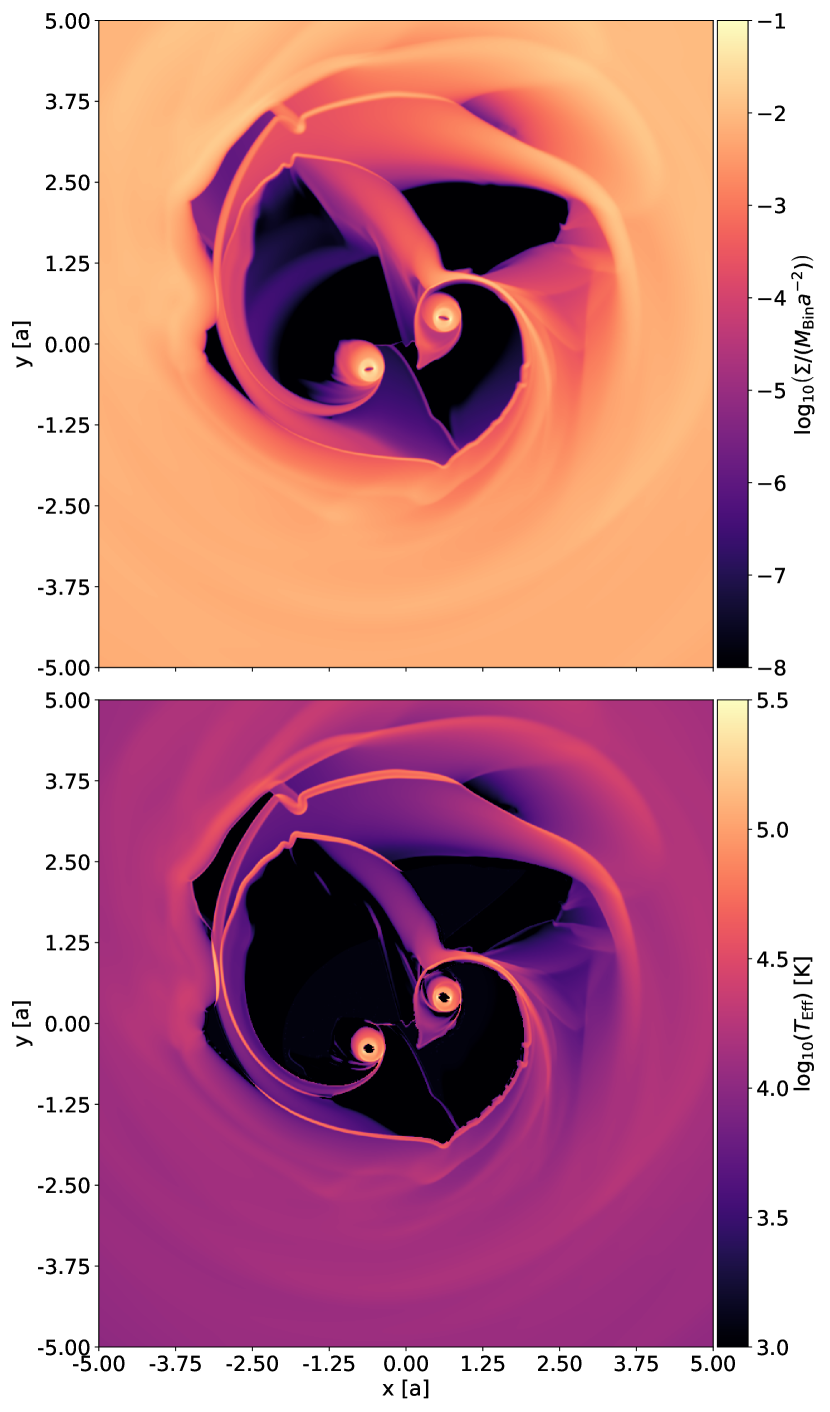
We begin by briefly recapitulating the most striking features present in a hydrodynamic simulation of a MBHB embedded in a CBD. Similar features have been found in many previous studies. Fig. 1 displays representative snapshots of the surface density and effective temperature distributions for the , , GR case.
We note the presence of an under-dense central region, often referred to as a central cavity. The sharp outer edge of this region is the cavity wall. Inside the cavity, there are accretion disks surrounding each of the individual BHs, called “mini-disks.” Lastly, note the central cavity is not entirely evacuated but is instead filled with distinct, extended filaments of gas. These filaments, or “streams,” are generated by the binary’s gravitational influence, which tends to peel gas from the cavity wall and produce these streams (D’Orazio et al., 2013).
Finally, we note that the hottest regions in our simulation domain are the mini-disks, with effective temperatures of . However, we also note that regions where the streams collide with each other or with the cavity wall are hot as well, with . The rest of the gas in our simulation remains at a relatively uniform .
3.1. Cavity features
| GR Precession | (, ) | (, ) | (, ) | ||||
|---|---|---|---|---|---|---|---|
| Yes | |||||||
| No | |||||||
| Yes | |||||||
| No | |||||||
| Yes | |||||||
| No |
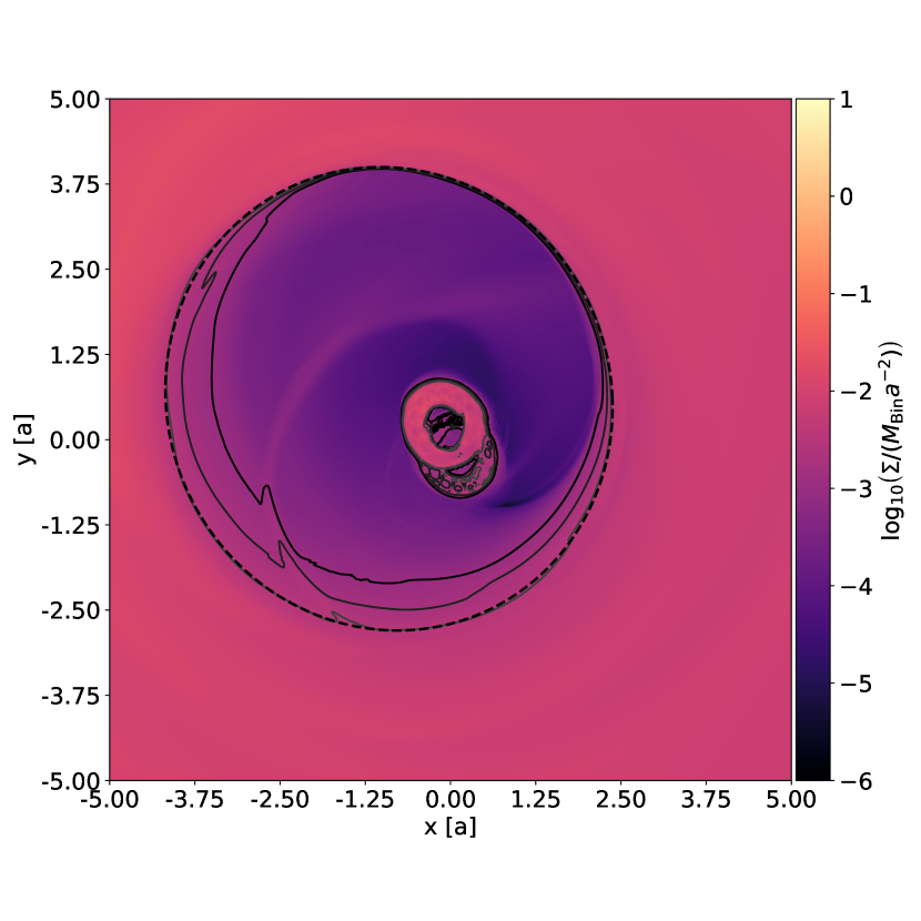
Note how the propagating tidal streams in Fig. 1 make it difficult to visualize the cavity. However, by time-averaging the surface density over a binary orbit, we reveal the cavity’s average properties more clearly. We describe the time-averaged cavity geometrically by fitting an ellipse to the and surface-density contour for and simulations, respectively. These density contours provide good qualitative representations of the cavity in each case – see the example in Fig. 2. In Table 2, we detail the median parameter values of these ellipses.
From Table 2 and Fig. 2, it is clear that the cavity properties are unique to each simulation, changing with the binary’s eccentricity, semi-major axis,333Although length scales in our simulations are normalized to the initial binary semi-major axis, the system is not scale-free with respect to it because the radiative cooling term described in Sec. 2.3 breaks scale symmetry. and equations of motion. A general understanding of how the cavity’s geometrical shape responds to different initial binary conditions is beyond the scope of this paper. Nevertheless, we describe the correlations we find in our simulations.
We first note that cavity size shows some correlation with binary eccentricity, with the simulations having larger cavity semi-major and semi-minor axes than the simulations. We also find that the simulations are more symmetric, in the sense that the center of the cavity is less offset from the binary’s barycenter, when compared to the simulations. We also note that none of the cavities are centered about the binary barycenter, and their semi-major axes are not oriented along the binary’s semi-major axis.
3.2. Cavity evolution
Next, we describe how the orbit-averaged cavity features of the simulations evolve over time—the features of the cavities are detailed in Sec. 5.
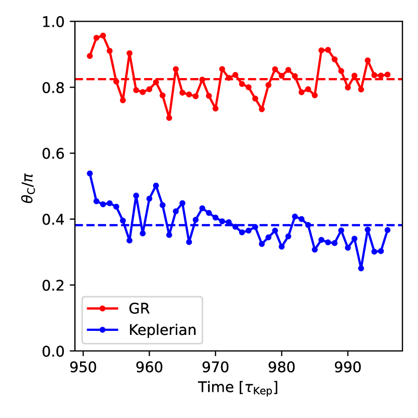
First, we note that the cavity semi-major axes in the runs are oriented in a constant direction. This is seen in both the GR and Keplerian runs and is depicted well in Fig. 3. Note how the orientation of the Keplerian and GR cavity, though noisy, both remain close to their median values, even though the binary semi-major axis of the GR simulation has precessed by an angle over a time we define to be (see Table 1 for values).
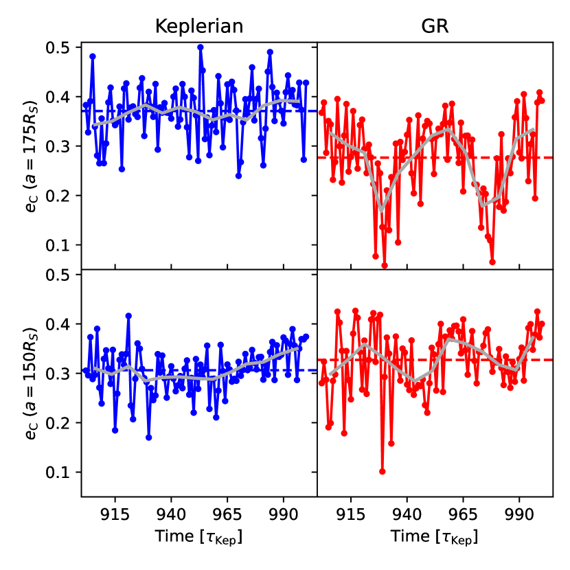
Although the orientation of the cavity’s semi-major axis () remains constant over time, the eccentricity of the cavity () does not, and appears to depend on the precession period. In Fig. 4, we display the eccentricity evolution of our simulations’ cavities. While all our simulations display some evolution, the GR simulations’ cavity eccentricities exhibit periodic oscillations on timescales of tens of binary orbits, whereas the Keplerian simulations’ are more or less constant, with no coherent trends. Further, we note that the amplitude of the periodicity is larger in the case (top right panel), which is the binary with slower GR precession. Finally, in both cases, we note that the period of this eccentricity oscillation agrees well with the precession periods of and , i.e. we measure peak periods of and for the and simulations, respectively.
Since the eccentricity-oscillation occurs only in the GR simulations, and has a period , it is clearly caused by the precession of the binary. However, the strength of the effect being anti-correlated with the precession rate is not as apparent. We suggest that the eccentricity modulation is caused by a similar mechanism that is responsible for the eccentricity growth of the Keplerian cavity. Hydraulic pumping (see Shi & Krolik 2015; Lai & Muñoz 2023) and eccentric Lindblad resonances (see Hirose & Osaki 1990; Lubow 1991a, b; Lai & Muñoz 2023) are both plausible causes, but the hydraulic pumping mechanism is particularly appealing due to the amplitude’s anti-correlation with precession rate.
For slower precession, the binary’s apocenter shifts less from one orbit to the next. Thus, consecutive streams are launched toward the cavity in a more coherent direction. Stream impacts on the cavity are more angularly coherent, pushing the impacted area of the cavity wall back further and driving stronger eccentricity modulations.
While further analysis of this mechanism remains outside the scope of this paper, in future work, we plan to investigate the effect of binary precession on the morphology and evolution of the cavity and, more broadly, of the circumbinary disk, especially since these could affect gas-torques on the binary, and may have significant effects on disk-induced binary orbital evolution.
4. Eccentric binaries
In the following section, we detail the key characteristics of our eccentric () binary simulations. In Sec. 4.1, we discuss the accretion rate of the system, demonstrating how its modulation is uniquely attributable to precession. In Sec. 4.2, we present and analyze the expected light-curves of the system, characterizing and determining the mechanism for both the long time-scale (tens of orbits) signal (Sec. 4.2.1) as well as the multiple individual flares (or sub-peak structures) that occur each orbit (Sec. 4.2.2). Throughout this section, we will conduct our analysis considering an MBHB in a static cavity. While this is not precisely the case, it is a helpful approximation for our simulations.
4.1. Accretion rate
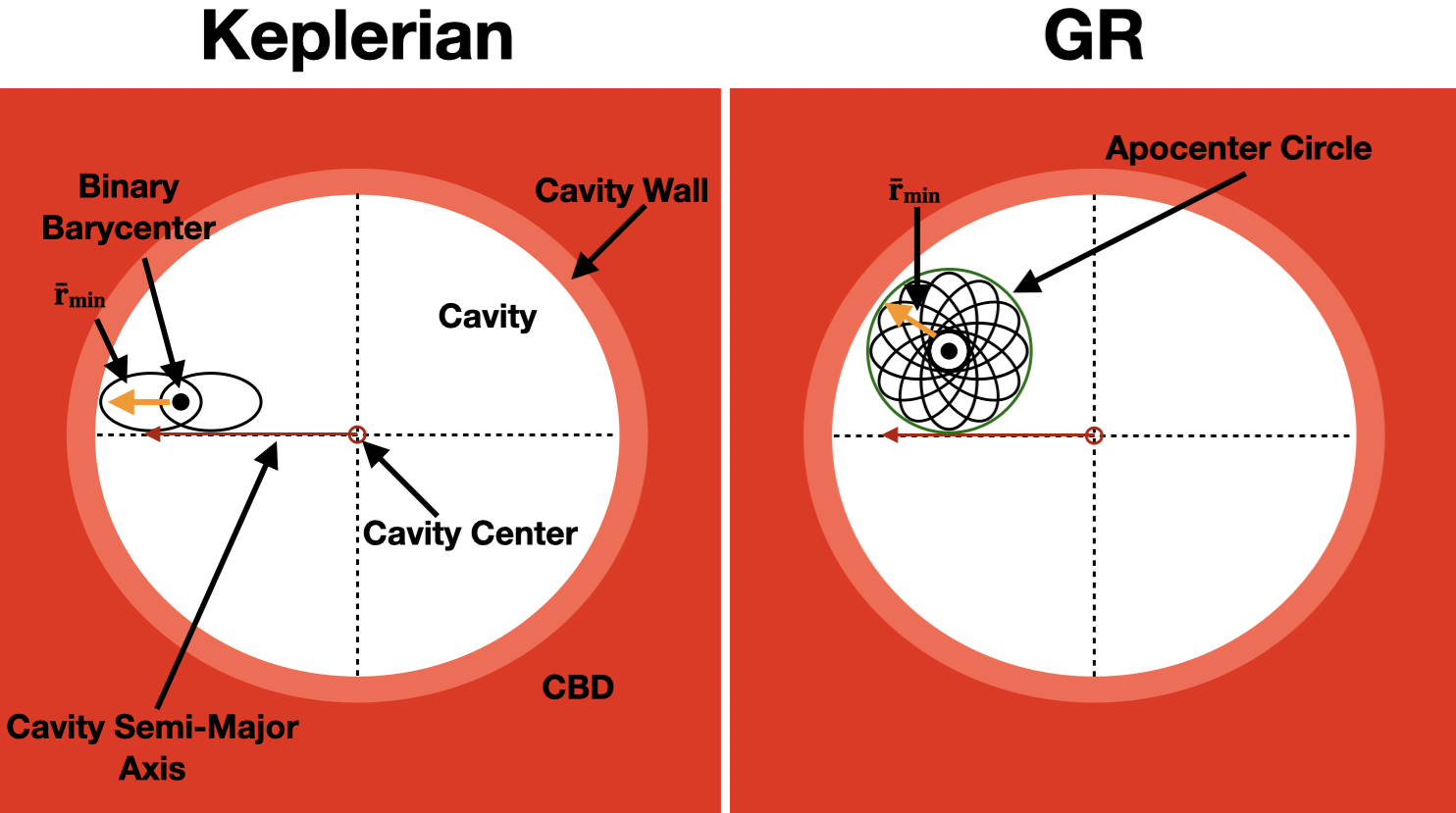
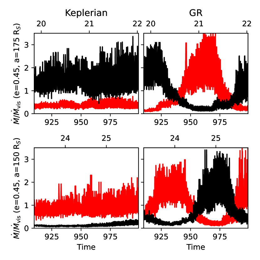
As illustrated in Table 2, the cavity center is offset from the binary barycenter in all of our simulations, meaning that the cavities are asymmetric about the BHs. This asymmetry introduces preferential accretion—where material prefers to accrete onto one BH over the other—in our system despite the black holes being the same mass. For a non-circular binary in an asymmetric cavity—in a binary orbit-averaged sense—one of the two BHs will always 444Over long time-scales we see a flip in which BH lies closer to the cavity and accretes at a higher rate. This is present in our simulations and has been reported in both Muñoz & Lai 2016 and Siwek et al. 2023a. lie closer to the cavity edge than the other, thereby having a stronger tidal pull and higher accretion rate than the other (see Fig. 5 and Siwek et al. 2023a). This “preferred” accretion onto one BH over the other is shown in Fig. 6.
Fig. 6 shows that our GR and Keplerian simulations display preferential accretion. However, unlike the Keplerian case, the GR simulation does not experience stable preferential accretion. Instead, the accretion rate for each BH varies periodically, with a stable amplitude and a period that is equal to twice the precession period (recall that, in our definitions, the precession period corresponds to the binary precessing by only radians). Further, we note that the two BHs’ accretion rates are out of phase with respect to one another. This behavior is due to the binary’s precession.
Unlike the Keplerian binary, the GR binary has a precessing apocenter that sweeps out a circle over its precession period (see Fig. 5). Since each apocenter on the circle is a different distance from the cavity wall, the BH’s tidal pull on the cavity will vary. As a result, each BH’s accretion rate varies quasi-sinusoidally with an angular period of and thereby a temporal period of . (We remind again that we defined as the time it takes to precess by , i.e., for the equal-mass BHs to “switch places”.) Further, since the BHs lie directly opposite to one other on the circle, their quasi-sinusoidal fluctuations have a phase difference of . The total binary accretion is the sum of the two fluctuating sinusoids with a period of , or , with an amplitude about half that of its components.
To determine when the binary experiences its peak accretion rate, we need to calculate when its tidal interaction with the cavity wall is strongest. We calculate the direction toward the cavity wall segment closest to the binary’s barycenter. This direction and distance is represented by the vector .
As noted in Table 2, the barycenters occupy different positions with respect to the cavity’s semi-major and semi-minor axes. For example, the barycenter of the binary is further offset from the cavity-center along the semi-minor axis, and less offset on the semi-major axis than that of the binary. These different barycenters change . Using the values from Table 2 we can calculate explicitly.
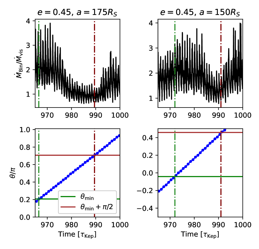
In Fig. 7, we display the binary accretion rate (black), the azimuthal position of a BH’s apocenter (blue), and we indicate both the azimuthal direction of , denoted as , and . We note that when the angle of a BH’s apocenter matches , that BH is closest to the cavity wall and thereby experiences peak accretion. The peak accretion rate of one BH is coincident with peak binary accretion due to the height of the peaks, as is easily inferred from Fig. 6. Similarly, when the binary semi-major axis is perpendicular to , binary accretion is at its minimum.
4.2. Light-curves
Using the post-processing technique discussed in Sec. 2.3, we generate expected light-curves for our binary systems, calculating the system’s bolometric, X-ray, UV, and optical luminosity. In the following section, we describe the amplitude and timing of their peaks, their characteristics in different bands, and their dependence on cavity geometry.
4.2.1 Long time-scale modulation
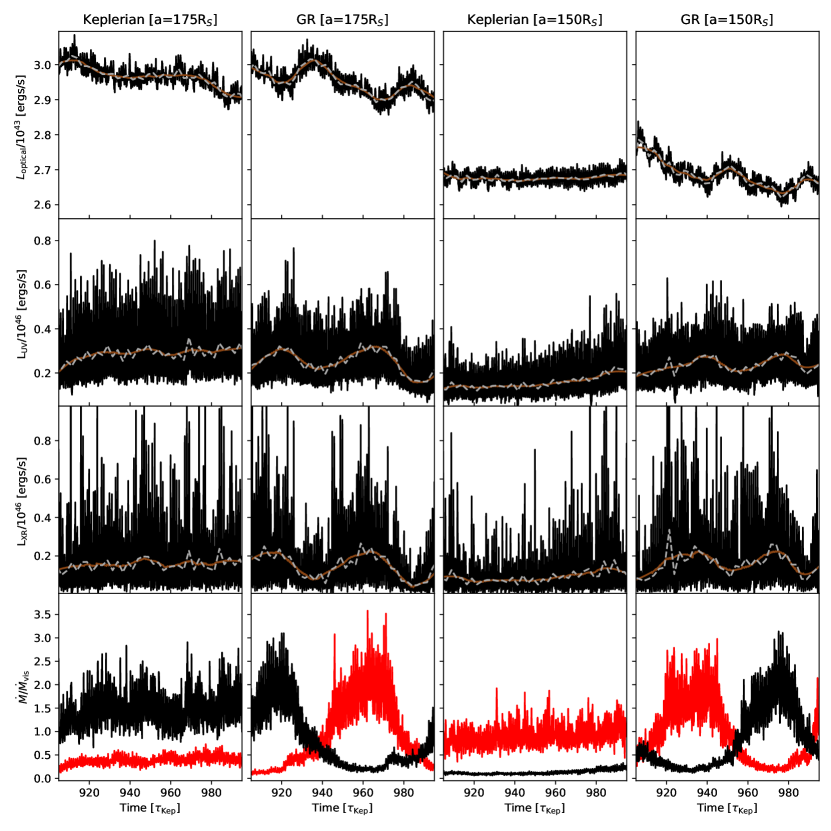
In Fig. 8, we show the accretion rates and light-curves for our simulations. First, we note that the X-ray and UV light-curves clearly track the behavior of the binary’s total accretion rate. The GR simulations exhibit simultaneous peaks and troughs, while the Keplerian simulations display simultaneous small upticks in the moving averages of , , and .
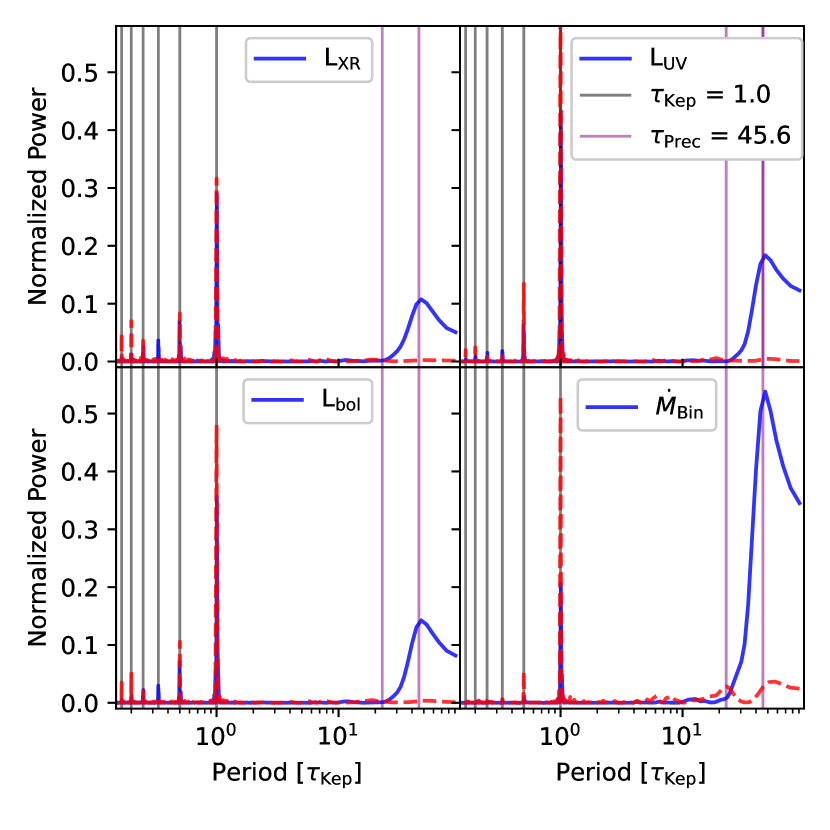
Though both simulations show that the X-ray and UV light-curves track binary accretion, we note that the GR and Keplerian simulations have notably different accretion rates and, thereby, different light-curves. We further delineate the characteristics of these signals by studying their Lomb-Scargle periodograms for the , case in Fig. 9.
In Fig. 9 we see two main peaks across all panels. The first is at and for the Keplerian and GR simulations, respectively. This peak is the orbital period of each binary. Though the orbital period for the GR binary () has a slightly longer period than its Keplerian counterpart—due to apsidal precesion—the periods are nearly indistinguishable in Fig. 9 and we only plot the Keplerian orbital period . The orbital period and its harmonics were previously reported in light-curves from non-precessing simulations (e.g. Westernacher-Schneider et al. 2022). However, unlike previous simulations, we note that Fig. 9 displays another peak at the precession period. This is a distinct signal unique to the GR case, at . We note that it is only second in power to the orbital frequency, making the possibility of observing it encouraging (see further discussion in Sec. 6 below).
While , , and are all similar to each other, has distinct behavior. In Fig. 8 the optical light-curves for the GR simulation show small amplitude peaks and troughs that are anti-correlated with those of , while those of the Keplerian simulations remain relatively flat. The explanation for the optical light-curves not being correlated with lies in the high temperature of the mini-disks.
In particular, the mini-disks are the hottest regions in our simulations (see map in Fig. 1), and thus have black-body spectra that are significantly biased towards the higher energy (X-ray and UV) bands. Thus, only the far tails of their emission are in the optical band. While the heating of the mini-disk causes significant modulations in the X-ray and UV luminosity, these modulations are weakly represented in the optical band. Thus, unlike the higher energy bands, whose light-curve modulations are tied to the gas fed to mini-disks through their interaction with the cavity wall, it is apparent that the flares in the optical light-curves do not. In the following section, we study these flares and the physical mechanism behind the light-curve shapes.
4.2.2 Flaring mechanisms
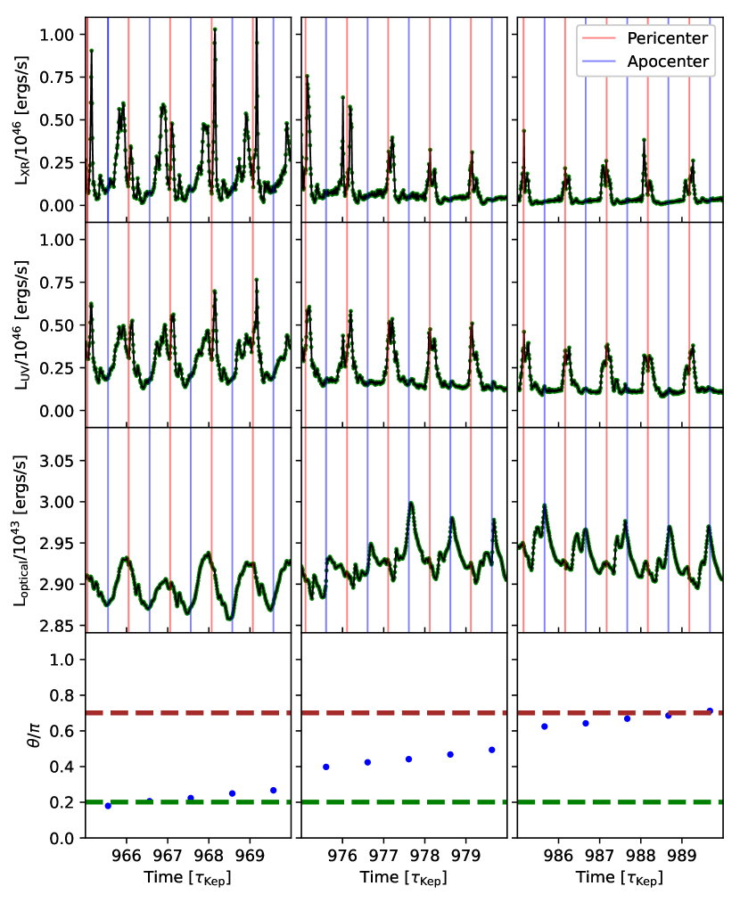
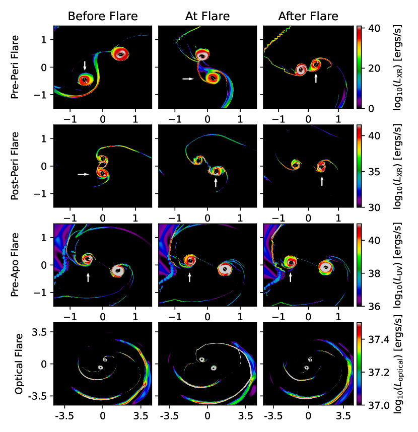
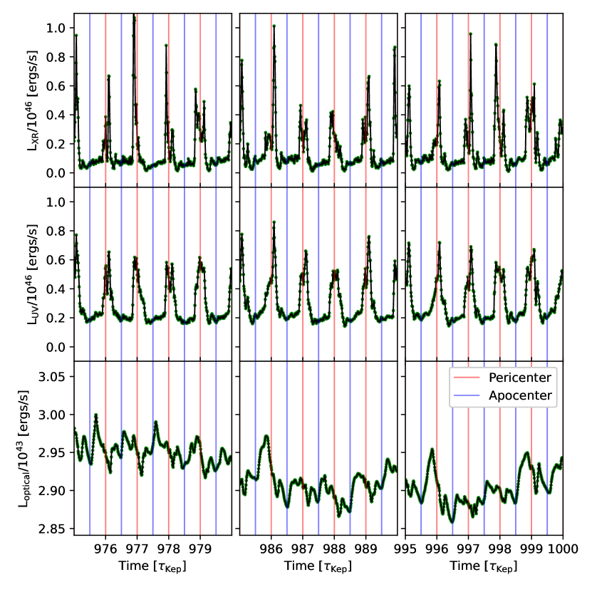
Fig. 10 displays zoom-in versions of the X-ray, UV, and optical light-curves for the , GR simulation. This figure shows three distinct flares per orbit in the X-ray and UV bands: one occurs just before each pericenter, another just after, and a third one roughly halfway between pericenter and apocenter. We will hereafter refer to these as “pre-peri”, “post-peri” and “pre-apo” flares. The optical band, on the other hand, displays a single distinct flare per orbit.
To investigate the physical mechanism behind this particular set of chromatic flares, we examine the system’s behavior before and after each of these flares in detail. Fig. 11 displays a series of snapshots of the surface luminosity density of the system just before, at, and just after each type of flare. The specific flaring instances displayed in Fig. 11 were arbitrarily chosen and are representative of large-amplitude instances of their respective type of flare.
The first (top) row shows snapshots around the pre-peri peak. Here, we see two BHs with distinct mindisks and a stream between them. The stream is generated from one BH’s interaction with the cavity wall (the BH indicated with an arrow). As the binary begins to approach its pericenter, the counterpart (upper) BH moves closer to the head of the stream, thereby exerting an increasingly strong gravitational pull on the stream. The head of the stream makes contact with the upper BH’s mini-disk, depositing enough gas to heat it significantly above the baseline temperature and luminosity, producing a flare. The top row middle panel of Fig. 11 highlights this deposition, illustrating how the luminous, heated material of the stream is being funneled onto the counterpart (upper) BH.
The second row shows snapshots around the post-peri peak. These reveal a tidal stripping of the mini-disks, somewhat analogous to Roche lobe overflow. Namely, we see the development of two streams reaching from one mini-disk to the other, forming a ‘double bridge’. As the BHs orbit, the two streams come closer together until they collide and form a single tidal bridge between the two BHs. This collision effectively squeezes the bridged material, pushing it towards each mini-disk, and causing a flare due to shock heating.
The third row shows snapshots around the pre-apo flare. These show the BH closer to the cavity wall (left) colliding with the low-luminosity wall. The resulting shock heats the BH’s tidal tail and the cavity wall, increasing the system’s luminosity and producing the flare.
The fourth and final row shows the snapshots around the time of our optical flare, notably the one at . As before, we note that the mini-disks’ luminosity do not strongly evolve throughout the flare. Instead, we observe a stream-cavity collision that causes the inner edge of the cavity wall to momentarily shine rather brightly, producing the optical flare we observe.
These mechanisms repeat and produce similar flares in each orbit. However, the amplitude and timing of these flares are not constant from orbit to orbit.
For example, the pair of pre- and post-peri flares decrease in amplitude and occur closer to each other in time as the binary’s accretion rate falls. As discussed above, this happens as the binary’s semi-major axis becomes more perpendicular to . This is evident when we compare flares from the first and third columns of Fig. 10. In the first column, the pre-peri and post-peri flares occur at and , a separation of . The third column, however, shows the pre-peri and post-peri flares at and , a much smaller separation of . Furthermore, the flares during high binary accretion are significantly brighter than those at low binary accretion. We note that the difference between the maximum luminosity of the two aforementioned pre-peri flares is . These effects are due to the changing tidal interaction between the BHs and the cavity, as discussed in the previous section and illustrated in Fig. 5.
More specifically, when the binary’s semi-major axis is aligned with , one BH is closer to and has a stronger tidal pull on the cavity, funneling significantly more gas to its mini-disk—this creates a large mini-disk and a small one. When the binary is more perpendicular to , neither BH is at its closest point to the cavity, and both have more equal tidal interactions with the cavity, leading to mini-disks that are, on average, both small and more equal in size. Furthermore, since the stream—relevant to the pre-peri flare—between the BHs is generated from the interaction of a BH with the cavity wall, it similarly is thinner, harboring less gas, when the binary is more perpendicular to .
We find that these differences in the mini-disk and stream size correspond to differences in the timing and amplitude of both the pre-peri and post-peri flares. With a thinner gas stream between the mini-disks, less disrupted stream material needs to travel further before depositing onto the edge of the mini-disk. Furthermore, smaller mini-disks sit deeper inside their host BH’s potential, requiring stronger tidal forces and smaller BH separation to facilitate the formation of a thinner mini-disk bridge. As a result, the amplitude of and time separation between the pair of pre-peri and post-peri flares are reduced as the binary becomes perpendicular to .
We also find long-term variations in the properties of the other two types of flares. The pre-apo flare steadily diminishes in amplitude until it is no longer discernible from the baseline emission - an example of this is seen at . The optical flare, on the other hand, both grows in amplitude and shifts its timing from pericenter to apocenter as the binary’s orbit becomes more perpendicular to . The cause for both of these behaviours can be attributed to the geometry of the system.
As the binary becomes more perpendicular to the apocenters of both BHs are no longer close enough to the cavity wall to collide with it and produce the pre-apo flare. As for the optical flare, we first note that tidal streams are launched perpendicular to the binary’s semi-major axis. Thus, when the binary is perpendicular to , the streams propagate in the direction parallel to . As a result, the streams travel a shorter distance and are less diffuse when they collide with the cavity, causing brighter flares closer to the previous pericenter from which they were launched.
Finally, we turn to Fig. 12, where we show the detailed light-curve of the Keplerian , simulation. As the figure reveals, we see the same types of flares in the X-ray and UV. They occur at the same points during the binary’s orbit and are caused by the same physical mechanisms. However, there is no significant change in the amplitude or timing of these flares in comparison to the GR case displayed in Fig. 10.
Indeed, the phenomena of tidal stripping, the formation of tidal streams, stream-cavity, and stream-mini-disk collisions are not unique to a precessing binary. Instead, they are generic to an eccentric binary that strongly interacts with an asymmetric cavity. On the other hand, the modulation in the amplitudes and timings of these flares are uniquely caused by the modulations in the accretion rate coming from the precession of the binary’s semi-major axis. Thus, the modulation in the amplitudes and timings of these flares is a GR effect.
5. Near-circular binaries
In the previous sections, we discussed the effects of GR precession in our simulations, detailing its signatures on accretion rates and light-curves. One expects such signatures to change qualitatively for sufficiently smaller eccentricity. In this section, we show that this qualitative change has already occurred by .
In the top panels of Fig. 13 we display the accretion rates in our simulations. Many of the characteristic signatures detailed in Sec. 4.1 are missing. Rather, in both the GR and Keplerian runs, we see comparatively mild preferential accretion and a binary accretion rate that has a starkly different time dependence in comparison with the binaries considered in previous sections. This accretion behavior and the corresponding features of the resulting light-curves are determined by the binary cavity geometry and the non-trivial evolution of the cavity itself. In the following sections, we detail these unique features in our simulations.
5.1. Binary-cavity interaction
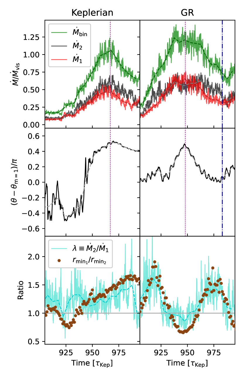
The first row in Fig. 13 displays the accretion rates in our two simulations, depicting , , in green, black, and red respectively. We see that the accretion rates on both BHs are fluctuating much less than for their counterparts. In fact, the BHs can accrete up to times the viscous inflow rate , which is times the maximum for the BHs—which only accrete up to each. The difference between the accretion rates of the two BHs in the case is also smaller than in the case. Where was for binaries, it is for binaries: an order of magnitude decrease. This reduction in accretion fluctuation and the accretion differential is chiefly due to the change in the binary’s apocenter with respect to the cavity.
As per Table 2, we note that the ellipses fit to the simulations’ cavities have centers that are much closer to the binary barycenter than that of the simulations, meaning that they are more symmetric about the barycenter. This reduces the differential between each BH’s distance to the cavity and, thereby, the differential in accretion rates. Further, binary apocenters scale with : the and binaries have apocenter values of and , respectively. Since a reduction in the radial extent of the binary increases the distance from both BHs to the cavity, there is a decrease in the maximum accretion rate–the amplitude of the fluctuation.
While the more circular shape of the binary orbit and the more central position of its apocenter help explain the simulations’ smaller accretion fluctuations and accretion differentials, they do not illuminate their particular time evolution. To do so, we must account for the cavity’s precession.
5.2. Cavity precession
An implicit assumption in Sec. 4 is that the orientation and shape of the cavity and the CBD are constant in time. However, the CBD can have a precession of its own. Recent studies have elucidated how CBD precession depends on binary eccentricity (Miranda et al., 2017; Siwek et al., 2023a; Tiede et al., 2023).
To characterize the precession of the cavity, we calculate the complex moment of the surface density
| (21) |
where we pick out the mode and define to have an origin about the barycenter. We compute the integral in Eqn. 21 over a radial annulus with an inner edge of and an outer edge of to fully capture the behavior of the asymmetric cavity and not be biased by behaviors in the outer disk. We have checked that our results are not sensitive to the precise definition of these boundaries.
The phase of the complex number defined in Eqn. 21, which we denote by , is used to characterize the inner CBD’s orientation and precession. The CBD’s orientation at a given time is given by the predominant value of around that time, whereas the CBD’s precession is given by a long-term linear trend in .555This phase is also a sensitive measure of waves propagating wave along the cavity wall. For example, the fast oscillations in the middle row of Fig. 13 have a period of roughly five orbits, and thus are likely the remnants of a “lump” phenomenon that is too weak to imprint noticeably on accretion rates, but can still be detected using the sensitive phase diagnostic (for examples of weak lump-like phenomena for eccentric binaries embedded in CBDs, see Westernacher-Schneider et al., 2022). We do this for each simulation snapshot, developing a time series of the mode’s azimuthal position.
The above procedure was performed on all our simulations. We found that while all our cavities experienced some precession, that of our simulations was insignificant. The highest cavity precession rate in our simulations was only and thus did not strongly affect our results. However, both simulations experience much faster cavity precession rates, with the highest cavity precession rate in our simulations being —over an order of magnitude increase. Despite having different thermodynamics, these results agree with previous models of Keplerian binary accretion by Miranda et al. 2017 and Tiede et al. 2023, which report that binaries have apsidally locked disks (i.e. they do not precess), and that binaries display strong disk precession. While a systematic study on how binary parameters affect the cavity’s precession remains beyond this paper’s scope, we will detail next how cavity precession affects accretion and the associated light-curves.
5.3. Binary accretion
In Sec. 4.1, we illustrated how the alignment between and the binary’s semi-major axis affects the accretion rate. We found that in a practically non-precessing cavity, when the binary semi-major axis aligns (anti-aligns) with , the binary accretion rate is at a maximum (minimum). When we account for the precession of the cavity, we find that the total accretion rate of the binary also depends on the binary’s relative position to the cavity.
We note that at each time step, the complex mode of the surface density defines a vector that points to the segment of the disk that is closest to the barycenter, essentially serving as a proxy for . Thus, in the middle panels of Fig. 13 we present the azimuthal position of the binary’s semi-major axis with respect to that of , an angle we will call the relative binary-cavity angle: .
It is clear from the figure that binary accretion closely tracks , with the two rising and falling together. For both the GR and the Keplerian simulation, we see that when is at a local maximum or minimum, so are the binary accretion rates. The purple (dotted) and blue (dash-dotted) vertical lines plotted in Fig. 13 highlight the coincidence of the peaks and valleys, respectively.
We further note that the accretion rates peak when and are lowest when . Equivalently, accretion is highest (lowest) when the binary semi-major axis and are anti-aligned (aligned). This is the opposite of our trend in Sec. 4.1.
The behaviour in Sec. 4.1 had an intuitive explanation: whenever the binary’s semi-major axis aligns with , one BH is closer to the cavity and thus the accretion rate of this BH spikes, while that of the other, more distant BH dips. If this were the dominant effect, then precession should cause the out-of-phase “see-saw” oscillations between vs. exhibited by the GR simulations in Sec. 4.1. However, for our much less eccentric binary, the accretion rates of the two BHs clearly vary in tandem, rather than out-of-phase. How can the behaviour be so different?
First, we note that for the above, the purely geometric modulation illustrated in Fig. 5 should occur for any value of the binary eccentricity. The amplitude of the see-sawing should scale monotonically with and become much less prominent in the case to the extent that the two accretion rates in the top panels of Fig. 13 are not strongly differentiated.
Second, we point out that while the cavity is more symmetric than its counterpart, it is still strongly lopsided, and its precession is not necessarily geometrically equivalent to the binary precession shown in Fig. 5. The precise shape of the cavity may evolve, and even for a fixed cavity shape, the precession may occur about a point that is offset from the barycenter. While we could not unambiguously diagnose such an offset, our results do suggest that as the cavity precesses, the closest distance from the binary’s barycenter to the cavity wall oscillates, modulating the accretion rates onto both BHs together. Furthermore, this modulation is apparently far dominant over the significantly dampened out-of-phase oscillations caused by the binary’s precession.
Finally, we note that binary accretion rates are largest when both BHs are roughly equidistant from the cavity wall and accreting close to equally (i.e. at ), and are smallest when one BH is closer to the cavity wall than the other and accreting unequally (i.e. at ).
5.4. Accretion ratio
In addition to the accretion ratio, we also show the ratio of the minimum distances from each BH to the cavity wall () in the bottom row of Fig. 13. Namely, we calculate for each BH using the ellipses fit to the surface-density contour, as originally described in Sec. 3. Despite the fact the cavity is not a perfect ellipse, which inherently limits the usefulness of , we find that the inverse ratio of the distances from the BHs to the cavity wall does, in fact, trace the general features in the evolution of the accretion ratio. As one BH gets closer to the cavity wall than the other, it accretes more than the other.
While low eccentricity binaries tend to have both BHs accrete relatively in phase, their accretion ratio is interestingly still dependent on the BHs’ relative distance to the nearest cavity wall. Thus, the geometric mechanism detailed in Fig. 5 is still present in the binary. However, the effect is significantly damped by smaller apocenter values.
5.5. Beat frequency
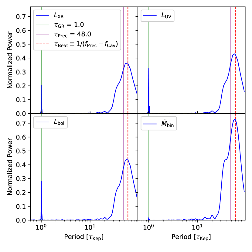
The GR simulation exhibits two precession periods: the apsidal precession of the binary and the precession of the cavity. The interplay between these precessions not only affects the accretion of the binary as shown in Fig. 13, but having two competing precession effects also imparts a dominant beat frequency into the accretion rate and associated light-curve signal.
In Fig. 14 we show the periodograms of , , , for our GR simulation. As before, we note that our system’s bolometric and high-energy bands are tied to the behavior of the mini-disks and thereby have similar periodograms to . However, unlike Fig. 9, we note that the luminosity periodograms do not peak around the binary precession period, but rather show a peak at the beat () between the binary precession period () and the period for the cavity to precess by (). Namely, from we determine that the period for the cavity to precess by is , which is quite similar to the values found by Siwek et al. 2023a and Miranda et al. 2017 in the isothermal case. We note that both precessions are prograde, and it is expected that the peak frequency would be the beat frequency since the beat frequency is simply the inverse of the cavity precession period if we were in the co-rotating frame of the binary. We also remind the reader that we defined the binary precession period to correspond to precession by radians, since for the equal-mass binaries we consider, the binary looks the same after half a rotation. For sufficiently unequal-mass binaries, one might instead expect a full precession of the binary to imprint on the dynamics.
6. Observability
In this section, we determine the parameter space where we could realistically hope to observe GR precession of the binary in EM and/or GW data. Namely, we require such systems to satisfy three constraints: (i) there are significant interactions between an eccentric binary and its CBD cavity, (ii) the binary has a sufficiently long GW-driven inspiral that is not exceedingly rare, and (iii) precession is fast enough for detection.
6.1. Cavity requirements
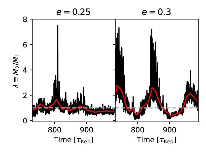
Much of the characteristic precession-based EM signatures we have detailed in Sec. 4.2 are dependent on strong interaction between the binary and the cavity wall (i.e large-amplitude quasi-sinusoidal ). The extent to which a binary interacts with the cavity wall depends on the choice of rather than . To determine the space where the binary interacts with the cavity strongly, we ran GR simulations with and with a step size of . We evolve each simulation as described in Sec. 2.5.
The accretion ratio is a sensitive diagnostic that can reveal subtle differences in the BH accretion rates. For example, indicates a sharp change in accretion behavior from to . In Fig. 15, we plot the accretion ratio of both simulations in black, overlaying the moving median with a window of in red. The differences between the panels in Fig. 15 are stark. The case does not display any periodicity, nor does the accretion ratio fluctuate significantly away from unity. The case, however, shows a clear large-amplitude oscillatory behavior. In fact we note that, as per Sec. 4.1, the period of its modulation is close to , where .
This pair of examples represents a genuine transition: the accretion ratio for binaries with are similar, and do not display a large-scale period or amplitude. The for simulations with eccentricities , however, all show periodicities on the time-scale of and with amplitudes monotonically increasing with —presumably due to the monotonically increasing value of their apocenters. Thus, we set as an eccentricity floor, at or below which binary eccentricity no longer interacts sufficiently strongly (for our purposes) with the cavity wall.
6.2. Timescale requirements
At the late stages of MBHB inspiral, the GW-driven inspiral outpaces the viscous timescale in the surrounding CBD. This was suggested, based on semi-analytic models, to lead to a “decoupling” of the binary from the disk (Liu et al., 2003; Milosavljević & Phinney, 2005; Haiman et al., 2009). Around this nominal decoupling time, two distinct effects may be expected: the binary may stop accreting from the disk, and the orbital evolution of the binary becomes dominated by GWs, rather than the gas disk. Recent hydrodynamical simulations (Farris et al., 2015b; Tang et al., 2017; Dittmann et al., 2023b; Krauth et al., 2023b; Franchini et al., 2024) addressed the first of these effects, and found that most binaries can accrete and remain luminous well past decoupling. Thus we do not consider the scenario where the binary no longer accretes from the disk. On the other hand, there remains an uncertainty about when and how the surrounding disk influences the orbital evolution of the binary.
As mentioned in Sec. 1, recent hydrodynamical simulations have also shown that a circumbinary disk induces an eccentricity of in the binary’s orbit (Muñoz et al., 2019; Zrake et al., 2021; Duffell et al., 2020; Siwek et al., 2023b). These simulations have not explicitly included the impact of GWs, i.e., they assumed the system is prior to any decoupling. Assuming that past the nominal decoupling, the GWs indeed dominate the orbital evolution, the orbits will rapidly circularize, reducing and ultimately eliminating relativistic precession effects.666In the presence of misaligned spins, there could still be precession, which we do not address in this paper.
Thus, to be conservative, we do not assume that the circumbinary disk influences our binary evolution, so we only account for GW decay. In light of this, we define timescale constraints that ensure that our binaries are common and long-lived, and that the EM precession signal we have detailed is observable. Namely, we place constraints on (i) the GW time to merger , (ii) the number of precession cycles the binary would exhibit in its lifetime defined by , and (iii) the length of the precession cycle .
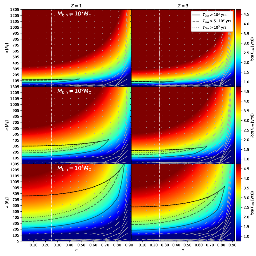
Specifically, we require years to observe at least several cycles on a human time scale. We also require to ensure that the binary would display enough cycles during its lifetime. Finally, we require to be greater than years, to ensure that these binaries are not exceedingly rare (characterised by the ratio of the merger time to quasar lifetime, see Xin & Haiman (2021)). The regions of parameter space that satisfy these constraints are enclosed by the black curves in Fig. 16.
In particular, we plot three curves, with each pertaining to one of the constraint values. The upper portion of these curves reflects the constraint of years (binaries need to be below this curve to precess fast enough). The lower portion of these curves reflects the constraint of years, respectively (binaries need to be above this curve to be common enough). Finally, we find that the condition for does not impose a strong constraint, only contributing the steeply upward sloping portion of the lower curve displayed exclusively for high and low values. The vertical white dot-dashed lines mark the binary eccentricity threshold of for strong interaction with the cavity, as discussed in Sec. 6.1.
We find that the region of observability expands as the binary mass decreases. This is largely due to requiring the precession timescale to be years. When normalized to orbital periods, only depends on , independent of binary mass at a constant separation . Since the orbital period, at a constant , increases with binary mass, we see the region of binaries with years expands dramatically with a decrease in mass. Furthermore, we see that the regions of observability shift slightly towards higher as the binary mass decreases. This is because increases with binary mass at a constant separation . Finally, we note that all regions shift to lower with an increase in .
The conclusion is that for binaries at , the largest observable region is a very narrow “sliver”, covering and . On the other hand, the chances of observing precession effects for a lower-mass system increase; for binaries, the largest observable region covers and . Furthermore, this trend extends outside the three binary masses we have specified in the panels. We find that systems are the most massive binaries that have a non-zero region which satisfies our most generous constraints, while lower-mass systems have continually expanding regions of observability, assuming that such intermediate-mass binaries exist and that they too are embedded in circumbinary disks.
Finally, as noted before, binaries shrink and circularize due to GW-driven decay. The gray line segments in Fig. 16 indicate the change of binary parameters over . While these evolutionary effects in the observable regions are slow enough not to interfere with the characterization of the signal, if the systems were to be observed for longer than 10 precession timescales, we would expect our precession signal’s period to lengthen and then, ultimately, disappear.
6.3. GW detections
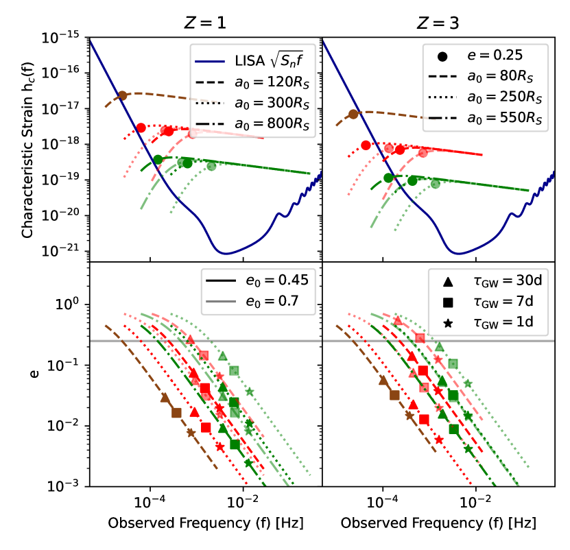
In the previous sections, we have outlined the necessary conditions for observing the effects of GR precession electromagnetically. While it may be challenging to identify the precession-induced modulations in the EM light-curve alone and to distinguish them from other sources of AGN variability, our system is also bright in gravitational waves. Thus, a GW detection followed up by observations in the X-ray and UV bands is likely to yield a much more robust determination of the mechanism driving the EM variability. The GR precession period is uniquely defined for , , , and , so if it is found imprinted on the EM light-curve, it can place excellent constraints on the binary parameters in combination with GW template searches. In Fig. 17 we illustrate the observability of our systems in GWs by initializing binaries with and values that satisfy our EM observability constraints and then calculating their characteristic strain and eccentricity as they shrink and circularize.
Namely, we calculate the characteristic amplitude or “strain” of the binary for the harmonic
| (22) |
where
| (23) | ||||
and
| (24) |
and is the luminosity distance to the source,
| (25) |
is the chirp mass, and
| (26) |
is the observed harmonic frequency (Peters & Mathews, 1963; Barack & Cutler, 2004; Enoki & Nagashima, 2007; Huerta et al., 2015).
In particular, Fig. 17 displays various binary systems’ strain and eccentricity evolution spanning mass, redshift, initial eccentricity, and initial semi-major axis. We only show the harmonics since these provide the highest strain in the parameter space displayed.
We find that at all our systems are loud enough to be detected by LISA and enter the LISA band just before they circularize to , the eccentricity floor we determined in Sec. 6.1. While more massive, initially less eccentric (), and wider () binaries enter the LISA band just before reaching this eccentricity, the remainder of our systems at are well within the band before they reach , i.e they are producing EM precession signals while being loud in LISA. A wide parameter space of , , and falls into this category at , spanning nearly three orders of magnitude in and up to in . We see a similar situation at , where most of our chosen systems produce an EM precession signal in the LISA band. However, due to the higher redshift, the strains are weaker, meaning that these systems produce the EM precession signal for less time in the LISA band.
While Fig. 17 only depicts a number of selected systems we note that the trends it displays can be extrapolated. The average strain increases monotonically with and with decreasing . We find that (i) systems with at are no longer detectable by LISA and (ii) the parameter space for systems producing a detectable EM precession signal while also detectable by LISA is greatly diminished at . Further, we note that an increase in shifts the strain curve towards lower frequencies, while a decrease in flattens the strain curve and shifts the eccentricity floor towards lower frequencies.
Though we only provide a sparse sampling of systems, the fact that a wide variety of binaries satisfy both EM and GW detection criteria through is encouraging for the prospect of identifying such sources in LISA and then following them up with EM observations to detect their EM precession signal.
7. Summary and conclusions
In this paper, we presented results from two-dimensional hydrodynamic simulations of general relativistic precessing equal-mass binaries in circumbinary disks. Our results not only have implications for the broad hydrodynamics of binaries in circumbinary disks, but they detail a new periodic EM signal that could be useful for multi-messenger searches for MBHBs. We list our main results below.
-
1.
We find that the apsidal precession of eccentric binaries () in CBDs creates a strong quasi-sinusoidal modulation in both the binary’s net accretion rate and in the accretion rate ratio of the individual binary components. The period of this modulation is the time it takes for the binary to precess by ().
-
2.
The X-ray and UV light-curves for eccentric, apsidally precessing binaries show corresponding quasi-sinusoidal modulations with a period of . This behavior contributes a low-frequency peak in the system’s periodogram that is second in strength only to the peak at the orbital frequency.
-
3.
Eccentric, apsidally precessing, massive () binary black holes at emit GWs whose harmonics are loud in LISA while simultaneously exhibiting this periodic EM signal.
-
4.
The X-ray and UV light-curves for eccentric binaries exhibit three flares per orbit with distinct hydrodynamic correlates. Apsidally precessing binaries uniquely display a periodic modulation in the amplitude and time separations of such flares.
-
5.
The optical light-curves for eccentric, apsidally precessing binaries do not share the accretion rate’s quasi-sinusoidal behavior. However, they display a periodic modulation in the timing of the orbital-frequency flare.
-
6.
The cavities around eccentric, apsidally precessing binaries experience periodic modulations in their eccentricities on the timescale . The amplitude of the modulation is anti-correlated with the binary precession rate, suggesting that the mechanism for the change in cavity eccentricity is stream-cavity collisions.
-
7.
Near-circular binaries exhibit significant cavity precession and, as a result, their accretion rate and light-curve signatures exhibit strong modulations with a frequency matching the beat frequency between the precession frequencies of the binary and the cavity.
-
8.
The accretion behavior of a MBHB system can be well encapsulated by tracking the distances from the BH to the closest segment of the cavity (). tracks , while the amplitude of and are dependent upon the values of and .
In future work, we plan to expand our current analysis to a larger set of binary parameters, running simulations with a broader range of eccentricities, precession rates, and mass ratios to better understand the processes at play. We also plan to further study the shape and time-evolution of the cavity in this broad range of parameter space so that the EM signals from near-circular binaries can be generically determined and, thus, included as candidates. Furthermore, we plan to calculate the effect of gas torques (in isothermal and gamma-law equations of state) and understand how apsidal precession of the binary would affect disk-induced binary evolution, such as the equilibrium values of the eccentricity and semi-major axis (Zrake et al., 2021; Duffell et al., 2020; Siwek et al., 2023b).
Finally, we are interested in determining the light-curves of the system when viewed along different lines of sight since preferential accretion suggests one mini-disk is brighter than the other, which would enhance a Doppler signal when not viewed face-on.
We conclude by noting that an apsidal precession of the binary imprints an additional periodic modulation in the X-ray and UV light-curves on the precession timescale of . This EM signature of precession may be observable for lower-mass MBHBs () that have a significant eccentricity (). With LISA triggers of sources up to we may be able to follow up on EM signals for a significant population of MBHBs—breaking degeneracies between the chirp mass, , , and other parameters. This novel multi-messenger signal has the potential to greatly refine our understanding of the eccentric binary black hole population, which hitherto has been poorly constrained by GWs alone.
Acknowledgments
We thank Daniel D’Orazio for valuable discussions. SD acknowledges financial support from the Gates-Cambridge Trust. ZH acknowledges financial support from NASA grants 80NSSC22K0822 and 80NSSC24K0440 and NSF grant AST-2006176. JD is supported by a Joint Columbia/Flatiron Postdoctoral Fellowship. Research at the Flatiron Institute is supported by the Simons Foundation. JZ acknowledges financial support from NASA grant 80NSSC24K0440. AM acknowledges financial support from NASA ATP grant 80NSSC22K0822. We also acknowledge computing resources from Columbia University’s Shared Research Computing Facility project, which is supported by NIH Research Facility Improvement Grant 1G20RR030893-01, and associated funds from the New York Empire State Development, Division of Science Technology and Innovation (NYSTAR) Contract C090171, both awarded April 15, 2010. This work made use of NASA-ADS. Software: Sailfish (Westernacher-Schneider et al., 2022), python (Oliphant, 2007; Millman & Aivazis, 2011), scipy (Jones et al., 2001), numpy (van der Walt et al., 2011), matplotlib (Hunter, 2007)
Data availability
The data underlying this article will be shared on reasonable request to the corresponding author.
References
- Agazie et al. (2023) Agazie G., et al., 2023, ApJ, 951, L8
- Amaro-Seoane et al. (2017) Amaro-Seoane P., et al., 2017, arXiv e-prints, p. arXiv:1702.00786
- Baker et al. (2019) Baker J., et al., 2019, BAAS, 51, 123
- Barack & Cutler (2004) Barack L., Cutler C., 2004, Physical Review D, 70
- Begelman et al. (1980) Begelman M. C., Blandford R. D., Rees M. J., 1980, Nature, 287, 307
- Blanchet (2002) Blanchet L., 2002, Living Reviews in Relativity, 5, 3
- Bode et al. (2012) Bode T., Bogdanović T., Haas R., Healy J., Laguna P., Shoemaker D., 2012, ApJ, 744, 45
- Bogdanović et al. (2008) Bogdanović T., Smith B. D., Sigurdsson S., Eracleous M., 2008, ApJS, 174, 455
- Bogdanović et al. (2022) Bogdanović T., Miller M. C., Blecha L., 2022, Living Reviews in Relativity, 25, 3
- Calcino et al. (2023) Calcino J., Dempsey A. M., Dittmann A. J., Li H., 2023, arXiv e-prints, p. arXiv:2311.13727
- Caprini & Figueroa (2018) Caprini C., Figueroa D. G., 2018, Classical and Quantum Gravity, 35, 163001
- Charisi et al. (2022) Charisi M., Taylor S. R., Runnoe J., Bogdanovic T., Trump J. R., 2022, MNRAS, 510, 5929
- Colpi et al. (2024) Colpi M., et al., 2024, arXiv e-prints, p. arXiv:2402.07571
- D’Orazio & Di Stefano (2018) D’Orazio D. J., Di Stefano R., 2018, Monthly Notices of the Royal Astronomical Society, 474, 2975
- D’Orazio et al. (2013) D’Orazio D. J., Haiman Z., MacFadyen A., 2013, MNRAS, 436, 2997
- D’Orazio et al. (2015) D’Orazio D. J., Haiman Z., Schiminovich D., 2015, Nature, 525, 351
- Davelaar & Haiman (2022a) Davelaar J., Haiman Z., 2022a, PhRD, 105, 103010
- Davelaar & Haiman (2022b) Davelaar J., Haiman Z., 2022b, Phys. Rev. Lett., 128, 191101
- Dittmann & Ryan (2021) Dittmann A. J., Ryan G., 2021, ApJ, 921, 71
- Dittmann et al. (2023a) Dittmann A. J., Dempsey A. M., Li H., 2023a, arXiv e-prints, p. arXiv:2310.03832
- Dittmann et al. (2023b) Dittmann A. J., Ryan G., Miller M. C., 2023b, ApJ, 949, L30
- Duffell et al. (2020) Duffell P. C., D’Orazio D., Derdzinski A., Haiman Z., MacFadyen A., Rosen A. L., Zrake J., 2020, ApJ, 901, 25
- Duffell et al. (2024) Duffell P. C., et al., 2024, arXiv e-prints, p. arXiv:2402.13039
- Enoki & Nagashima (2007) Enoki M., Nagashima M., 2007, Progress of Theoretical Physics, 117, 241
- Farris et al. (2014) Farris B. D., Duffell P., MacFadyen A. I., Haiman Z., 2014, ApJ, 783, 134
- Farris et al. (2015a) Farris B. D., Duffell P., MacFadyen A. I., Haiman Z., 2015a, MNRAS, 446, L36
- Farris et al. (2015b) Farris B. D., Duffell P., MacFadyen A. I., Haiman Z., 2015b, MNRAS, 447, L80
- Franchini et al. (2024) Franchini A., Bonetti M., Lupi A., Sesana A., 2024, A&A, submitted; e-print arXiv:2401.10331,
- Frank et al. (2002) Frank J., King A., Raine D. J., 2002, Accretion Power in Astrophysics: Third Edition. Cambridge University Press
- Giacomazzo et al. (2012) Giacomazzo B., Baker J. G., Miller M. C., Reynolds C. S., van Meter J. R., 2012, ApJ, 752, L15
- Gutiérrez et al. (2022) Gutiérrez E. M., Combi L., Noble S. C., Campanelli M., Krolik J. H., López Armengol F., García F., 2022, ApJ, 928, 137
- Haiman et al. (2009) Haiman Z., Kocsis B., Menou K., 2009, ApJ, 700, 1952
- Hassan & Rosen (2012) Hassan S. F., Rosen R. A., 2012, Phys. Rev. Lett., 108, 041101
- Hazboun et al. (2013) Hazboun J. S., Pichardo Marcano M., Larson S. L., 2013, arXiv e-prints, p. arXiv:1311.3153
- Hirose & Osaki (1990) Hirose M., Osaki Y., 1990, PASJ, 42, 135
- Hu et al. (2020) Hu B. X., D’Orazio D. J., Haiman Z., Smith K. L., Snios B., Charisi M., Di Stefano R., 2020, MNRAS, 495, 4061
- Huerta et al. (2015) Huerta E. A., McWilliams S. T., Gair J. R., Taylor S. R., 2015, Phys. Rev. D, 92, 063010
- Hunter (2007) Hunter J. D., 2007, Computing in Science and Engineering, 9, 90
- Ingram et al. (2021) Ingram A., Motta S. E., Aigrain S., Karastergiou A., 2021, Monthly Notices of the Royal Astronomical Society, 503, 1703
- Jones et al. (2001) Jones E., Oliphant T., Peterson P., et al., 2001, SciPy: Open source scientific tools for Python, http://www.scipy.org/
- Kelley et al. (2019) Kelley L., et al., 2019, BAAS, 51, 490
- Kocsis et al. (2008) Kocsis B., Haiman Z., Menou K., 2008, ApJ, 684, 870
- Krauth et al. (2023a) Krauth L. M., Davelaar J., Haiman Z., Westernacher-Schneider J. R., Zrake J., MacFadyen A., 2023a, arXiv e-prints, p. arXiv:2310.19766
- Krauth et al. (2023b) Krauth L. M., Davelaar J., Haiman Z., Westernacher-Schneider J. R., Zrake J., MacFadyen A., 2023b, MNRAS, 526, 5441
- Lai & Muñoz (2023) Lai D., Muñoz D. J., 2023, ARA&A, 61, 517
- Liu et al. (2003) Liu F. K., Wu X.-B., Cao S. L., 2003, MNRAS, 340, 411
- Lubow (1991a) Lubow S. H., 1991a, ApJ, 381, 259
- Lubow (1991b) Lubow S. H., 1991b, ApJ, 381, 268
- Millman & Aivazis (2011) Millman K. J., Aivazis M., 2011, Computing in Science & Engineering, 13, 9
- Milosavljević & Phinney (2005) Milosavljević M., Phinney E. S., 2005, ApJ, 622, L93
- Miranda et al. (2017) Miranda R., Muñoz D. J., Lai D., 2017, MNRAS, 466, 1170
- Muñoz & Lai (2016) Muñoz D. J., Lai D., 2016, ApJ, 827, 43
- Muñoz et al. (2019) Muñoz D. J., Miranda R., Lai D., 2019, ApJ, 871, 84
- Oliphant (2007) Oliphant T. E., 2007, Computing in Science & Engineering, 9, 10
- Paschalidis et al. (2021) Paschalidis V., Bright J., Ruiz M., Gold R., 2021, ApJ, 910, L26
- Peters & Mathews (1963) Peters P. C., Mathews J., 1963, Phys. Rev., 131, 435
- Robson et al. (2019) Robson T., Cornish N. J., Liu C., 2019, Classical and Quantum Gravity, 36, 105011
- Schutz (1986) Schutz B. F., 1986, Nature, 323, 310
- Shakura & Sunyaev (1973) Shakura N. I., Sunyaev R. A., 1973, A&A, 24, 337
- Shi & Krolik (2015) Shi J.-M., Krolik J. H., 2015, ApJ, 807, 131
- Siwek et al. (2023a) Siwek M., Weinberger R., Muñoz D. J., Hernquist L., 2023a, MNRAS, 518, 5059
- Siwek et al. (2023b) Siwek M., Weinberger R., Hernquist L., 2023b, MNRAS, 522, 2707
- Tang et al. (2017) Tang Y., MacFadyen A., Haiman Z., 2017, MNRAS, 469, 4258
- Tiede et al. (2023) Tiede C., D’Orazio D. J., Zwick L., Duffell P. C., 2023, arXiv e-prints, p. arXiv:2312.01805
- Westernacher-Schneider et al. (2022) Westernacher-Schneider J. R., Zrake J., MacFadyen A., Haiman Z., 2022, Phys. Rev. D, 106, 103010
- White & Rees (1978) White S. D. M., Rees M. J., 1978, MNRAS, 183, 341
- Xin & Haiman (2021) Xin C., Haiman Z., 2021, Monthly Notices of the Royal Astronomical Society, 506, 2408–2417
- Zrake et al. (2021) Zrake J., Tiede C., MacFadyen A., Haiman Z., 2021, ApJ, 909, L13
- de Rham et al. (2018) de Rham C., Melville S., Tolley A. J., 2018, Journal of High Energy Physics, 2018, 83
- van der Walt et al. (2011) van der Walt S., Colbert S. C., Varoquaux G., 2011, Computing in Science and Engineering, 13, 22