Long-range wormhole teleportation

Abstract

We extend the protocol of Gao and Jafferis (2021) to allow wormhole teleportation between two entangled copies of the Sachdev-Ye-Kitaev (SYK) model Sachdev and Ye (1993); Kitaev (2015) communicating only through a classical channel. We demonstrate in finite $N$ simulations that the protocol exhibits the characteristic holographic features of wormhole teleportation discussed and summarized in Jafferis et al. (2022). We review and exhibit in detail how these holographic features relate to size winding which, as first shown by Brown et al. (2021), Nezami et al. (2021), encodes a dual description of wormhole teleportation.

QCCFP Collaboration

I Introduction

Building on the work of Gao et al. (2017), Maldacena et al. (2017), and others Maldacena (2003); Hayden and Preskill (2007); Sachdev (2010); Shenker and Stanford (2014a, b); Maldacena and Stanford (2016); Susskind (2016); Susskind and Zhao (2018); Susskind (2017), the wormhole teleportation protocol developed by Gao and Jafferis (2021) is a concrete realization of the $ER$$=$$EPR$ hypothesis of Maldacena and Susskind (2013). The protocol consists of a series of quantum gate operations, of the type routinely performed now in the laboratory on various kinds of quantum processors. Importantly there is a well-defined semi-classical limit in which this teleportation protocol has an equivalent holographic description as coherent transmission of quantum states through a traversable wormhole.

The basic semi-classical picture resembles an Einstein-Rosen bridge connecting two black holes. In the traversable wormhole teleporation protocol Gao and Jafferis (2021) the role of the two black holes is played by two entangled copies of the Sachdev-Ye-Kitaev (SYK) model Sachdev and Ye (1993); Kitaev (2015). The SYK model is a quantum mechanical system of $N$ Majorana fermions interacting $q$ at a time in all possible combinations with Hamiltonian:

$$H_{L,R}=\sum_{1\leq j_{1}<\dots<j_{q}\leq N}J_{j_{1}\dots j_{q}}\psi^{\ell,r}_{j_{1}}\dots\psi^{\ell,r}_{j_{q}},$$ (1)

where we use the Left-Right symbols $L,R$ to distinguish the two SYK copies with Majorana fermions corresponding labeled by $\ell,r$. The couplings $J_{j_{1}\dots j_{q}}$ are the same for both copies, and are drawn randomly from a Gaussian distribution with mean zero and variance

$$\langle\left(J_{j_{1}\dots j_{q}}\right)^{2}\rangle=\frac{2^{q-1}(q-1)!}{qN^{q-1}}{\cal J}^{2}$$ (2)

where ${\cal J}$ is a coupling constant with dimensions of energy. The SYK Hamiltonian resembles the dynamics of a black hole in that it is an efficient scrambler. Scrambling in this context refers to the fact that quantum information injected into the system via a simple operator rapidly delocalizes into multipartite entanglement. One can track scrambling via operator growth over time. Like black holes, the SYK model saturates the upper bound on the Lyapunov exponent describing operator growth Maldacena et al. (2016); Maldacena and Stanford (2016), in the limit $N$$\to$$\infty$, $\beta{\cal J}$$\to$$\infty$, $N/\beta{\cal J}$$\to$$\infty$.

The dynamics of the SYK model has no spatial dependence, and the action of Majorana fermion operators in zero spatial dimensions is equivalent to strings of Pauli operators via the Jordan-Wigner transformation. As a result the quantum dynamics of SYK could be realized on a variety of digital or analog quantum processors independently of the details of the hardware implementation. To the extent that one can then invoke a holographic description of wormhole teleportation as traversing a wormhole, the space being traversed is not the space of the laboratory, but rather an emergent space arising from the dynamics of quantum entanglement. This makes wormhole teleportation a promising window for probing features of quantum gravity away from the semi-classical regime.

It was demonstrated in Gao and Jafferis (2021) that, in a semi-classical limit with $N$$\to$$\infty$, $q$$\to$$\infty$, $\beta{\cal J}$$\to$$\infty$, traversable wormhole teleportation can have perfect fidelity, and exhibits a number of qualitative features related to the holographic description with a wormhole. The most obvious of these is that, unlike the standard Alice-Bob teleportation protocol Bennett et al. (1993) employed in quantum networks (see, e.g. Valivarthi et al. (2020)) wormhole teleportation completes after a dynamically determined time interval, equivalent in the dual description to the time taken, as measured by an external observer, to transit the wormhole. In Jafferis et al. (2022) it was shown, both explicitly on a quantum processor and in more detail in a simulation on a classical computer, that several qualitative features of wormhole teleportation persist well away from the semi-classical regime (e.g. $N$$=$$10$, $q$$=$$4$, $\beta{\cal J}$$=$$4$), at the expense of reduced fidelity.

An additional complication noted in Gao and Jafferis (2021) is that when the holographic teleportation has less than perfect fidelity, it competes with other non-holographic effects. The first is a “direct swapping” of quantum information intrinsic to the protocol, which dominates at early times and degrades rapidly due to the same scrambling dynamics that induce wormhole teleportation at its characteristic time scale. The second is a many-body effect, dubbed “peaked-size teleportation” in Schuster et al. (2022), which always dominates at late times after the characteristic completion time of the wormhole teleportation, as well as at infinite temperature. An additional possible mechanism, not seen in the examples discussed in this paper, is “teleportation through thermalization”, a many-body mechanism discussed recently in Gao (2023).

The wormhole teleportation protocol of Gao and Jafferis (2021) includes applying, over some time interval, an explicit unitary operator exp$(i\mu V)$ connecting the two entangled SYK systems. Here $\mu$ is a coupling constant and $V$ is proportional to a sum of Majorana fermion bilinears $\psi^{\ell}_{j}\psi^{r}_{j}$. In the holographic description this interaction introduces a negative energy pulse resulting in a Shapiro advance that makes the wormhole traversable; this in turn implies the requirement that the coupling constant $\mu$ must be negative. As already observed in Gao et al. (2017), Maldacena et al. (2017), and Gao and Jafferis (2021), traversability of the wormhole does not uniquely determine the form of the Left-Right interaction.

The wormhole teleportation described so far has a key difference from the standard Alice-Bob teleportation that prevents it from operating between separated systems. Standard Alice-Bob teleportation is based on an entangled Bell pair shared between Alice and Bob. In that protocol Alice performs a Bell state measurement jointly on her qubit and a second message qubit; she then calls Bob via a classical channel and instructs him to perform particular gate operations on his qubit, the choice of which depends on Alice’s measurement outcome. The teleportation of the message qubit completes successfully, without any quantum interaction between Alice and Bob. The wormhole teleportation protocol described in Gao and Jafferis (2021) and performed on a Sycamore quantum processor Jafferis et al. (2022) has no classical channel; it resembles instead a variation of the standard Alice-Bob protocol (see, e.g., Lykken (2021)) where Alice’s measurement and the classical channel to Bob is replaced by a quantum channel consisting of two control gates (CNOT and CZ) that directly connect Alice and Bob. The quantum channel consists entirely of control gates with Alice’s qubits as the controls, hence the deferred measurement principle Nielsen and Chuang (2012) guarantees that the two protocols achieve identical results.

The wormhole teleportation protocol in Gao and Jafferis (2021) does not have an equivalent variant using a classical channel because of the particular form chosen for the Left-Right coupling $V$. Thus to achieve long-range wormhole teleportation we need to first modify $V$. We use a modified Left-Right coupling suggested by Nezami et al. (2021) (see also Maldacena et al. (2017) and Kourkoulou and Maldacena (2017)) and demonstrate that we can still achieve wormhole teleportation with the previously identified holographic features. As a final step we modify the protocol to make use of a classical channel.

The outline of this paper is as follows. In section II we establish notation and review the basics of the wormhole teleportation protocol of Gao and Jafferis (2021). In section III we warm up with the case of the Gao-Jafferis protocol at infinite temperature and no time allowed for scrambling; here the final state can be computed analytically. We observe no wormhole teleportation but instead the Left-Right interaction induces a Left-Right swap, leading to nonzero quantum information transfer. This is sufficient to see explicitly that the protocol of Gao and Jafferis (2021) cannot be replaced with a long-range classical channel. In section IV we replace the Left-Right interaction operator $V$ with a different operator $V^{b}$, and show that the basic features of traversable wormhole teleportation also appear in this modified protocol. We show that the Left-Right swap is absent for this long-range protocol. In section V we review the size winding description of traversable wormhole teleportation, and demonstrate how it works using either the operator $V$ or the operator $V^{b}$ to define “size”. We show that both cases exhibit an approximate $SL(2,R)$ symmetry, which is closely related to size winding in the holographic description Maldacena and Qi (2018); Brown et al. (2021); Nezami et al. (2021). From the size winding analysis we are able to extract finite-$N$ Lyapunov exponents and compare them to the semi-classical limit. In section VI we discuss the holographic feature of causal time ordering, and show that it occurs in the long-range teleportation protocol. In section VII we demonstrate how to further modify the protocol to include a classical channel. This involves measurement of Alice’s qubits on the left, and displays some interesting features of multipartite entanglement. Finally, in section VIII we discuss the possibility and challenges of implementing long-range wormhole teleportation on quantum hardware, perhaps over quantum networks currently under development. We provide in Appendix B a comparison between the SYK-based protocols discussed here and the commuting models recently studied by Gao (2023).

II Notation and definitions

We choose units such that $\cal{J}$$=$$\hbar$$=$$c$$=$1, thus when we write time $t$ as a dimensionless number we actually mean $t\cal{J}/\hbar$, and when we write the inverse temperature $\beta$ as a dimensionless number we actually mean $\beta$$\cal{J}$.

We mostly use the notation and conventions of Gao and Jafferis (2021). The two entangled SYK systems each have $N$ Majorana fermions; we label Alice’s by $\psi^{\ell}_{i}$ and Bob’s by $\psi^{r}_{i}$, $i=0,\ldots N$$-$$1$. The Majorana operator normalization is implied by the anti-commutation relations:

$$\{\psi^{\ell}_{i},\psi^{\ell}_{j}\}=\{\psi^{r}_{i},\psi^{r}_{j}\}=\delta_{ij}$$ (3)

Expectation values at $\beta$$=$$0$ are taken with respect to the maximally entangled state $\ket{I}$ that satisfies

$$\psi^{\ell}_{j}\ket{I}=-i\psi^{r}_{j}\ket{I}\;;\quad\psi^{r}_{j}\ket{I}=i\psi^{\ell}_{j}\ket{I}$$ (4)

for all of the left and right Majoranas $\psi^{\ell}_{j}$, $\psi^{r}_{j}$, $j=0,\ldots,N$$-$$1$. At finite $\beta$ and $t$$=$$0$ we will take expectation values with respect to the normalized thermofield double state $\ket{\rm tfd}$ defined by

$$\ket{\rm tfd}\equiv\rho_{\beta}^{1/2}\ket{I}=Z^{-1/2}_{\beta}{\rm e}^{-\beta H_{L}/2}\ket{I}=Z^{-1/2}_{\beta}{\rm e}^{-\beta H_{R}/2}\ket{I}$$ (5)

where $\beta$ is the inverse temperature, $Z_{\beta}$ is the corresponding partition function, and we have used the fact that $(H_{L}-H_{R})\ket{I}=0$.

The wormhole teleportation protocol of Gao and Jafferis (2021) introduced an explicit coupling between the left and right Majoranas exp$(i\mu V)$, where the Hermitian operator $V$ is defined by

$$V=i\sum_{j=0}^{N-1}\,\psi^{\ell}_{j}\psi^{r}_{j}$$ (6)

and $\mu$ is a coupling constant. In the simplest version of the protocol this interaction is applied at a single time slice $t$$=$$0$, but we will also consider, following Jafferis et al. (2022), extending the interaction over multiple time steps. Note that in Gao and Jafferis (2021) $V$ was defined with an additional factor of $1/(qN)$. This means that to compare a $\mu$ value used here to a $\mu$ value in Gao and Jafferis (2021), one should first multiply it by $qN$. Our convention for $\mu$ matches with Gao (2023).

The quantum information to be teleported initially resides in a Bell state pair of qubits denoted $R$,$Q$, and the goal is to transfer the quantum information to a readout qubit $T$. At some “injection time” $-t_{0}$ we want to swap the qubit $Q$ with one of the qubits implementing the Left SYK dynamics, and at the “extraction time” $t_{1}$ we need to swap out into $T$ from one of the qubits that implement the Right SYK dynamics. The wormhole teleportation protocol uses the following complex fermions for swapping:

$$\chi_{\ell}=\frac{1}{\sqrt{2}}\left(\psi^{\ell}_{0}+i\psi^{\ell}_{1}\right)\;;\quad\{\chi_{\ell},\chi_{\ell}^{\dagger}\}=1\;;\quad\chi_{\ell}^{2}=(\chi_{\ell}^{\dagger})^{2}=0$$ (7)

$$\chi_{r}=\frac{1}{\sqrt{2}}\left(\psi^{r}_{0}+i\psi^{r}_{1}\right)\;;\quad\{\chi_{r},\chi_{r}^{\dagger}\}=1\;;\quad\chi_{r}^{2}=(\chi_{r}^{\dagger})^{2}=0$$ (8)

As in eqn. 2.6 of Gao and Jafferis (2021), the Left swap operation $S_{Q\ell}$ from the qubit Q into the Left Majoranas, and the Right swap operation $S_{Tr}$ from the Right Majoranas into the readout qubit T, are given by:

$$S_{Q\ell}=\begin{pmatrix}1&0\\ 0&0\end{pmatrix}_{Q}\otimes\chi_{\ell}\chi_{\ell}^{\dagger}+\begin{pmatrix}0&1\\ 0&0\end{pmatrix}_{Q}\otimes\chi_{\ell}^{\dagger}+\begin{pmatrix}0&0\\ 1&0\end{pmatrix}_{Q}\otimes\chi_{\ell}+\begin{pmatrix}0&0\\ 0&1\end{pmatrix}_{Q}\otimes\chi_{\ell}^{\dagger}\chi_{\ell}$$ (9)

$$S_{Tr}=\begin{pmatrix}1&0\\ 0&0\end{pmatrix}_{T}\otimes\chi_{r}\chi_{r}^{\dagger}+\begin{pmatrix}0&1\\ 0&0\end{pmatrix}_{T}\otimes\chi_{r}^{\dagger}+\begin{pmatrix}0&0\\ 1&0\end{pmatrix}_{T}\otimes\chi_{r}+\begin{pmatrix}0&0\\ 0&1\end{pmatrix}_{T}\otimes\chi_{r}^{\dagger}\chi_{r}$$ (10)

The initial $RQ$ state is taken to be the Bell state $(\ket{00}+\ket{11})/\sqrt{2}$, while the initial state of the readout qubit $T$ is $\ket{0}$. The full quantum state at time $t$$=$$0$ is thus the following tensor product state with $N$$+$$3$ qubits:

$$\ket{t=0}=\frac{1}{\sqrt{2}}(\ket{00}+\ket{11})\otimes\ket{\rm tfd}\otimes\ket{0}$$ (11)

and the wormhole teleportation protocol produces the following final state:

$$\ket{\rm final}=S_{Tr}\,{\rm e}^{-iH_{R}t_{1}}\,{\rm e}^{i\mu V}\,{\rm e}^{-iH_{L}t_{0}}\,S_{Q\ell}\,{\rm e}^{iH_{L}t_{0}}\ket{t=0}$$ (12)

Thus, starting at $t$$=$$0$, we time evolve backwards with the Left SYK hamiltonian to the injection time $-t_{0}$, swap in the quantum information of qubit $Q$, time evolve back to $t$$=$$0$, apply the Left-Right interaction, time evolve with the Right SYK hamiltonian to the extraction time $t_{1}$, then swap out into the readout qubit $T$. In the holographic picture the two copies of the SYK system (Left and Right) time evolve together and, as for the Einstein-Rosen bridge, forward time evolution with $H_{L}$ is like backward time evolution with $H_{R}$, thus what $H_{L}$ scrambles, $H_{R}$ unscrambles. In the protocol we only include the pieces of the time evolution that affect the teleportation outcome.

As shown in Gao and Jafferis (2021), it follows that the reduced density matrix of $TR$ in the final state is given by:

$$\rho_{TR}=\frac{1}{2}\begin{pmatrix}\rho_{11}&0&0&\rho_{14}\\ 0&\rho_{22}&\rho_{23}&0\\ 0&\rho_{23}^{*}&\rho_{33}&0\\ \rho_{14}^{*}&0&0&\rho_{44}\end{pmatrix}$$ (13)

where here we have absorbed the time evolution into $\chi_{\ell}$$\to$$\chi_{\ell}(-t_{0})$, $\chi_{r}$$\to$$\chi_{r}(t_{1})$, and where

$$\rho_{11} =\left\langle\chi_{\ell}\chi_{\ell}^{\dagger}\,{\rm e}^{-i\mu V}\chi_{r}\chi_{r}^{\dagger}\,{\rm e}^{i\mu V}\chi_{\ell}\chi_{\ell}^{\dagger}\right\rangle+\left\langle\chi_{\ell}^{\dagger}\,{\rm e}^{-i\mu V}\chi_{r}\chi_{r}^{\dagger}\,{\rm e}^{i\mu V}\chi_{\ell}\right\rangle$$

$$\rho_{14} =\left\langle\chi_{\ell}\,{\rm e}^{-i\mu V}\chi_{r}^{\dagger}\,{\rm e}^{i\mu V}\chi_{\ell}\chi_{\ell}^{\dagger}\right\rangle+\left\langle\chi_{\ell}^{\dagger}\chi_{\ell}\,{\rm e}^{-i\mu V}\chi_{r}^{\dagger}\,{\rm e}^{i\mu V}\chi_{\ell}\right\rangle$$

$$\rho_{22} =\left\langle\chi_{\ell}\,{\rm e}^{-i\mu V}\chi_{r}\chi_{r}^{\dagger}\,{\rm e}^{i\mu V}\chi_{\ell}^{\dagger}\right\rangle+\left\langle\chi_{\ell}^{\dagger}\chi_{\ell}\,{\rm e}^{-i\mu V}\chi_{r}\chi_{r}^{\dagger}\,{\rm e}^{i\mu V}\chi_{\ell}^{\dagger}\chi_{\ell}\right\rangle$$

$$\rho_{23} =\left\langle\chi_{\ell}\chi_{\ell}^{\dagger}\,{\rm e}^{-i\mu V}\chi_{r}^{\dagger}\,{\rm e}^{i\mu V}\chi_{\ell}^{\dagger}\right\rangle+\left\langle\chi_{\ell}^{\dagger}\,{\rm e}^{-i\mu V}\chi_{r}^{\dagger}\,{\rm e}^{i\mu V}\chi_{\ell}^{\dagger}\chi_{\ell}\right\rangle$$ (14)

$$\rho_{33} =\left\langle\chi_{\ell}\chi_{\ell}^{\dagger}\,{\rm e}^{-i\mu V}\chi_{r}^{\dagger}\chi_{r}\,{\rm e}^{i\mu V}\chi_{\ell}\chi_{\ell}^{\dagger}\right\rangle+\left\langle\chi_{\ell}^{\dagger}\,{\rm e}^{-i\mu V}\chi_{r}^{\dagger}\chi_{r}\,{\rm e}^{i\mu V}\chi_{\ell}\right\rangle$$

$$\rho_{44} =\left\langle\chi_{\ell}\,{\rm e}^{-i\mu V}\chi_{r}^{\dagger}\chi_{r}\,{\rm e}^{i\mu V}\chi_{\ell}^{\dagger}\right\rangle+\left\langle\chi_{\ell}^{\dagger}\chi_{\ell}\,{\rm e}^{-i\mu V}\chi_{r}^{\dagger}\chi_{r}\,{\rm e}^{i\mu V}\chi_{\ell}^{\dagger}\chi_{\ell}\right\rangle$$

Figure 1 shows results typical of the wormhole teleportation protocol at finite $N$. Plotted is the mutual information $I(R$$:$$T)$ (in units of log2) between the qubits $R$ and $T$ as a function of time, averaged over 10 instantiations of the SYK model random couplings, and taking the injection and extraction times to be equal in magnitude: $t_{0}$$=$$t_{1}$. The figure shows results for both negative and positive values of the Left-Right interaction coupling $\mu$. The quantum information shared between $R$ and $T$ has three different contributions: (i) holographic wormhole teleportation, which produces a peak in the mutual information at a characteristic time, but only when $\mu$ is chosen negative; (ii) non-holographic direct swapping of quantum information between the Left and Right systems, described in detail in the next section, which occurs maximally for $t_{0}=t_{1}=0$ and is symmetric under the sign chosen for $\mu$; (iii) non-holographic many-body “peaked-size teleportation” , discussed in detail in subsection V.2, which occurs maximally at late times and is symmetric under the sign chosen for $\mu$.

As seen in Figure 1, for $N$$=$$10$ and 14 there is substantial variation in the mutual information plot from different instantiations, although they are qualitatively similar. For $N$$=$$24$ this variation disappears; this is a result of the well-studied self-averaging property of the SYK model Garcia-Garcia and Verbaarschot (2016); Cotler et al. (2017). We take advantage of this property in our analysis to construct and study examples using a single instantiation of the SYK couplings .

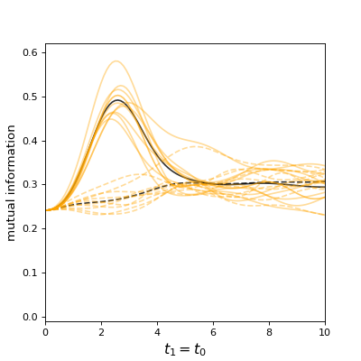
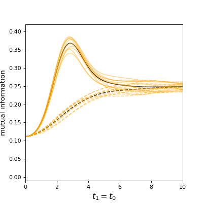
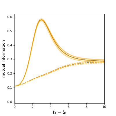
Figure 1: Left: Mutual information (computed using the second Renyi entropies) between the qubits $R$ and $T$ after running the wormhole teleportation protocol with injection at time $-t_{0}$ and extraction at time $t_{1}$$=$$t_{0}$. Results from ten instantiations of the $N$$=$$10$ SYK model with $q$$=$$4$, $\cal J$$=$$1$, $\beta$$=$$4$, using the Left-Right interaction $V$ with coupling $\mu$$=$$-0.3$ (solid)/$\mu$$=$$+0.3$ (dashed). The orange lines are the individual instantiations, and the black lines are the mean. Middle: The same for $N$$=$$14$, except $\mu$$=$$\pm 0.2$. Right: The same for $N$$=$$24$, except $\mu$$=$$\pm 0.2$.

III Warm up exercise: the Gao Jafferis protocol with $t_{0}$$=$$t_{1}$$=$$\beta$$=$$\mathrm{𝟎}$

For $t_{0}$$=$$t_{1}$$=$$\beta$$=$$0$ we compute the reduced density matrix for the reference and readout qubits $RT$ explicitly as a function of the interaction strength $\mu$. Starting from eqn. 13, and using the identities given in Appendix A, the result is:

$$\rho_{TR}(t=0,\beta=0)=\frac{1}{2}\begin{pmatrix}\frac{1}{2}(1+{\rm sin}^{2}\mu)&0&0&{\rm sin}\mu\\ 0&\frac{1}{2}(1-{\rm sin}^{2}\mu)&0&0\\ 0&0&\frac{1}{2}(1-{\rm sin}^{2}\mu)&0\\ {\rm sin}\mu&0&0&\frac{1}{2}(1+{\rm sin}^{2}\mu)\end{pmatrix}$$ (15)

from which the further reduced density matrices of $R$ and $T$ follow:

$$\rho_{R}(t=0,\beta=0)=\rho_{T}(t=0,\beta=0)=\frac{1}{2}\begin{pmatrix}1&0\\ 0&1\end{pmatrix}$$ (16)

We compute the corresponding mutual information $I(R$$:$$T)$ using the second Renyi entropies:

$$I(R:T) =S(R)+S(T)-S(RT)$$

$$={\rm log}_{2}\left(\frac{{\rm Tr}(\rho_{RT}^{2})}{{\rm Tr}(\rho_{R}^{2}){\rm Tr}(\rho_{T}^{2})}\right)$$

$$=2\,{\rm log}_{2}\left(1+{\rm sin}^{2}\mu\right)$$ (17)

We find that $I(R$$:$$T)$ vanishes for $\mu$$=$$0$ (i.e. no Left-Right interaction), and is maximal, $I(R$$:$$T)$$=$$2$ in units of log(2), for $|\mu|$$=$$\pi/2$. This phenomenon has nothing to do with wormhole teleportation or any other kind of teleportation, as we demonstrate below.

The Left-Right interaction is written explicitly as a unitary gate operation on qubits. We represent the Left Majoranas $\psi_{0}^{\ell}$, and $\psi_{1}^{\ell}$ as acting on the same left qubit $\ell$, and the Right Majoranas $\psi_{0}^{r}$, and $\psi_{1}^{r}$ as acting on the same Right qubit $r$, as the following Pauli matrix operators:

$$\psi_{0}^{\ell} =\frac{1}{\sqrt{2}}X^{\ell}\;;\quad\quad\quad\psi_{1}^{\ell}=\frac{1}{\sqrt{2}}Y^{\ell}$$

$$\psi_{0}^{r} =\frac{1}{\sqrt{2}}Z^{\ell}X^{r}\;;\quad\quad\psi_{1}^{r}=\frac{1}{\sqrt{2}}Z^{\ell}Y^{r}$$ (18)

where the Pauli $Z$ matrices are needed, as per Jordan-Wigner, to enforce anti-commutation.

It follows that

$$V_{01}=\frac{1}{2}\left(Y^{\ell}X^{r}-X^{\ell}Y^{r}\right)$$ (19)

so

$${\rm e}^{i\mu V_{01}}=\left({\rm cos}\frac{\mu}{2}\,{\cal I}_{4}+i\,{\rm sin}\frac{\mu}{2}\,Y^{\ell}X^{r}\right)\left({\rm cos}\frac{\mu}{2}\,{\cal I}_{4}-i\,{\rm sin}\frac{\mu}{2}\,X^{\ell}Y^{r}\right)$$ (20)

where ${\cal I}_{4}$ is the 4d identity matrix. We can write this more explicitly as the following 2-qubit unitary gate operation:

$${\rm e}^{i\mu V_{01}}=\begin{pmatrix}1&0&0&0\\ 0&{\rm cos}\mu&{\rm sin}\mu&0\\ 0&-{\rm sin}\mu&{\rm cos}\mu&0\\ 0&0&0&1\end{pmatrix}$$ (21)

It is instructive to rewrite this as a product of two unitary operators:

$${\rm e}^{i\mu V_{01}}=\begin{pmatrix}1&0&0&0\\ 0&1&0&0\\ 0&0&-1&0\\ 0&0&0&1\end{pmatrix}\cdot\begin{pmatrix}1&0&0&0\\ 0&{\rm cos}\mu&{\rm sin}\mu&0\\ 0&{\rm sin}\mu&-{\rm cos}\mu&0\\ 0&0&0&1\end{pmatrix}$$ (22)

The reader can easily check that the first matrix is the 2-qubit entangling operation CNOT$\cdot$CZ$\cdot$CNOT, with the Left qubit $\ell$ as the control. The second matrix, for $\mu$$=$$\pi/2$, is the canonical 2-qubit SWAP gate:

$${\rm SWAP}=\begin{pmatrix}1&0&0&0\\ 0&0&1&0\\ 0&1&0&0\\ 0&0&0&1\end{pmatrix}$$ (23)

The presence of swapping implies that this transfer of quantum information cannot be interpreted as teleportation: the deferred measurement principle does not apply to swapping; this is easily seen explicitly by writing the SWAP operator as three successive CNOTs with control and target qubits alternating. Thus we cannot use a classical channel to reproduce the same effect.

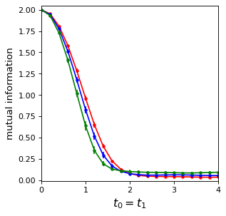
Figure 2: Time dependence of the direct transmission mechanism. Mutual information $I(R$$:$$T)$ after running the wormhole teleportation protocol with injection at time $-t_{0}$ and extraction at time $t_{1}$$=$$t_{0}$. The red/blue/green points are results averaging 10 instantiations of the $N$$=$$10$ SYK model with Left-Right interaction $V$, using $\cal J$$=$$1$, and $\beta$ = 0,4, and 16 respectively. We have chosen $|\mu|$$=$$\pi/2$ so that the direct transmission has perfect fidelity for $t_{0}$$=$$t_{1}$$=$$0$.

Even in this simple example with $\mu$$=$$\pi/2$ we also see a more general puzzle related to implementing a classical channel, arising from the Pauli $Z$ operations needed to enforce anti-commutation of the Right Majoranas with the Left Majoranas. These imply that the operator $S_{Tr}$ is not just the canonical 2-qubit SWAP gate applied to qubits $T$ and $r$, but also acts on the Left qubit $\ell$.

$${\rm S_{Tr}}={\rm CZ}(T\to\ell)\cdot{\rm CZ}(r\to\ell)\cdot{\rm SWAP}(Tr)$$ (24)

where the direction of the arrows in the CZ gate go from the control qubit to the target qubit. This feature, which will appear in any implementation of wormhole teleportation using fermions, appears at first glance to be an obstacle to implementing a classical channel. Fortunately we can use the fact that for any pair of qubits $a$,$b$, CZ($a$$\to$$b$) = CZ($b$$\to$$a$), thus

$${\rm S_{Tr}}={\rm CZ}(\ell\to T)\cdot{\rm CZ}(\ell\to r)\cdot{\rm SWAP}(Tr)$$ (25)

This means, again appealing to the deferred measurement principle, that the CZ gates can be replaced by a classical channel between Alice and Bob. In fact, only the first CZ gate has an effect on $I(R$$:$$T)$; the second one can be dropped.

As a final insight from this example, we study the case of $\mu$$=$$\pi/2$ when we go to finite temperature and some range of nonzero time evolution. Figure 2 shows results using the Left-Right interaction $V$ and three different values of $\beta$: 0, 4, and 16. We use $|\mu|$$=$$\pi/2$ so that the direct transmission has perfect fidelity for $t_{0}$$=$$t_{1}$$=$$0$ and thus dominates over any teleportation effect at early times. We see that the direct transmission effect drops off rapidly with time, becoming negligible for $t\gtrsim 2$, although a small residual remains. The rapid falloff is due to the efficient scrambling from the SYK Hamiltonian. As expected, the characteristic time scale for the swapping effect to become negligible is roughly the same as the timescale for the wormhole teleportation to turn on.

IV Long-range protocol

Consider replacing the Left-Right interaction exp$(i\mu V)$ with exp$(i\mu V^{b})$, where $V^{b}$ is defined by

$$V^{b}=\sum_{j=0}^{N/2-1}\,\Gamma^{(2)\ell}_{j}\Gamma^{(2)r}_{j}$$ (26)

where

$$\Gamma^{(2)\ell}_{j}=2i\psi^{\ell}_{2j}\psi^{\ell}_{2j+1}\;;\quad\Gamma^{(2)r}_{j}=2i\psi^{r}_{2j}\psi^{r}_{2j+1}$$ (27)

We can give an alternate expression for $V^{b}$ by substituting a Jordan-Wigner representation on $N$ qubits for the $2N$ Majoranas:

$$\psi_{2j}^{\ell} =\frac{1}{\sqrt{2}}Z_{0}\ldots Z_{j-1}X_{j}\;;\quad\psi_{2j+1}^{\ell}=\frac{1}{\sqrt{2}}Z_{0}\ldots Z_{j-1}Y_{j}\;;\quad j=0,1,\ldots N/2-1$$

$$\psi_{2j}^{r} =\frac{1}{\sqrt{2}}Z_{0}\ldots Z_{j-1+N/2}X_{j+N/2}\;;\quad\psi_{2j+1}^{r}=\frac{1}{\sqrt{2}}Z_{0}\ldots Z_{j-1+N/2}Y_{j+N/2}$$ (28)

From which we see that:

$$V^{b}=\sum_{j=0}^{N/2-1}\,Z_{j}Z_{j+N/2}$$ (29)

Eqn. 29 is the expression proposed originally by Nezami et al. (2021).

IV.1 Absence of direct transmission in the long-range protocol

If we replace $V$ by $V^{b}$, the computation of the matrix elements in equations II becomes trivial. This is because of the identities:

$${\rm e}^{-i\mu V_{01}^{b}}\,\Gamma_{0}^{(2)r}\,{\rm e}^{i\mu V_{01}^{b}}=\Gamma_{0}^{(2)r}\;;\quad\quad{\rm e}^{-i\mu V_{01}^{b}}\,\chi_{r}^{\dagger}\,{\rm e}^{i\mu V_{01}^{b}}=-\chi_{r}^{\dagger}$$ (30)

from which we derive:

$$\rho_{RT}(t=0,\beta=0)=\frac{1}{2}\begin{pmatrix}\frac{1}{2}&0&0&0\\ 0&\frac{1}{2}&0&0\\ 0&0&\frac{1}{2}&0\\ 0&0&0&\frac{1}{2}\end{pmatrix}$$ (31)

which implies $I_{RT}(t$$=$$0,\beta$$=$$0)=0$.

Another way to see this is to observe that:

$${\rm e}^{i\mu V_{01}^{b}} ={\rm cos}\mu\,{\cal I}_{4}+i\,{\rm sin}\mu\,\Gamma_{0}^{(2)\ell}\Gamma_{0}^{(2)r}$$

$$={\rm cos}\mu\,{\cal I}_{4}+i\,{\rm sin}\mu\,Z^{\ell}Z^{r}$$ (32)

$$=\begin{pmatrix}{\rm e}^{i\mu}&0&0&0\\ 0&{\rm e}^{-i\mu}&0&0\\ 0&0&{\rm e}^{-i\mu}&0\\ 0&0&0&{\rm e}^{i\mu}\end{pmatrix}$$

which, unlike the expression in eqn 21, is obviously not a Left-Right swap.

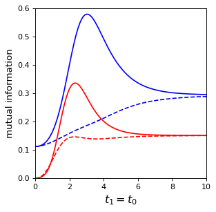
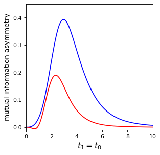
Figure 3: Left: mutual information (computed using the second Renyi entropies) between the qubits $R$ and $T$ after running the wormhole teleportation protocol with injection at time $-t_{0}$ and extraction at time $t_{1}$$=$$t_{0}$. Results from a single instantiation of the $N$$=$$24$, $q$$=$$4$, SYK model with $\beta$$=$$4$, $\cal J$$=$$1$, using either the Left-Right interaction $V$ (blue lines) with $\mu$$=$$-0.2$ (solid)/$\mu$$=$$+0.2$ (dashed), or $V^{b}$ (red lines) with the same values of $\mu$. Right: the asymmetry in the $RT$ mutual information between using negative/positive values of the coupling $\mu$ in the protocol.

IV.2 Quantum information transfer with the long-range protocol

Figure 3 compares the results of the original wormhole teleportation protocol using $V$ and the modified protocol using $V^{b}$. In both cases we take $N$$=$$24$, $q$$=$$4$, $\beta$$=$$4$, ${\cal J}$$=$$1$, and $\mu=\pm 0.2$. As previously remarked, using $V^{b}$ there is no direct transmission, so the mutual information vanishes at $t_{0}$$=$$0$. Instead, as $t_{0}$ is increased, we observe a smooth ramp up of the holographic contribution, leading to a mutual information peak only for negative $\mu$, and the non-holographic contribution from the “peaked-size teleporation”, that approaches the same late time asymptotic value for either sign of $\mu$. The fact that the mutual information between qubits $R$ and $T$ develops a substantial time-dependent asymmetry, depending on whether the sign of $\mu$ corresponds to a negative versus positive energy pulse in the holographic picture, is a signature feature of wormhole teleportation, and as we demonstrate in section V agrees with the time evolution of the size winding. The overall transfer of quantum information is less efficient using $V^{b}$ rather than $V$; this is consistent with the differences in the efficiency of the size winding shown in the next section.

V Size winding

Size winding Brown et al. (2021); Nezami et al. (2021) is a key feature of wormhole teleportation. It directly relates a coherent property of the operator spreading induced by SYK scrambling dynamics to motion along the emergent light cone through the traversable wormhole Maldacena et al. (2017),Maldacena and Qi (2018),Lin et al. (2019). The holographic duality of wormhole teleportation is precisely the statement that the complete size winding description and the through-the-wormhole description have a mapping into each other. In this sense it is reasonable to use the size winding description as our definition of what we mean by traversable wormhole behavior away from semi-classical regime. Note, however, that the presence of individual components of the size winding description does not necessarily imply a holographic dual.

V.1 Review of size winding with the Gao-Jafferis protocol

We briefly review the size winding mechanism and demonstrate how it works in simulations using the original Gao-Jafferis protocol with Left-Right interaction $V$.

A single Majorana fermion $\psi_{i}^{\ell}$, $\psi_{i}^{r}$ in the Left or Right SYK systems will time evolve as

$$\psi_{i}^{\ell}(t)={\rm e}^{iH_{L}t}\psi_{i}^{\ell}{\rm e}^{-iH_{L}t}\;;\quad\psi_{i}^{r}(t)={\rm e}^{iH_{R}t}\psi_{i}^{r}{\rm e}^{-iH_{R}t}\$$ (33)

We can expand either of these in the terms of the the complete set of left/right basis operators $\Gamma_{J}^{(s)\ell}$,$\Gamma_{J}^{(s)r}$ as defined, e.g. in Qi and Streicher (2019); Gao (2023):

$$\Gamma^{(s)}_{J}=2^{s/2}i^{s(s-1)/2}\psi_{j_{1}}\ldots\psi_{j_{s}}$$ (34)

where $J$ represents the string of ordered indices $j_{1}$,$j_{2}$,$\dots j_{s}$ labeling some combination of $s$ Majoranas. These basis operators are Hermitian, square to the identity, and create mutually orthogonal states acting on $|I\rangle$. Note also the relation:

$$\Gamma^{(s)\ell}_{J}\ket{I}=(-i)^{s}\Gamma^{(s)r}_{J}\ket{I}$$ (35)

The scrambling dynamics of the SYK model imply that over time $\psi_{i}^{\ell}(t)$ and $\psi_{i}^{r}(t)$ will have support on a larger and larger number of basis operators. Since each basis operator is a string of $s$ Majoranas, the effective size of $\psi_{i}^{\ell}(t)$ and $\psi_{i}^{r}(t)$ will grow over time. To study this in more detail, it is useful to follow Qi and Streicher (2019) and do the same expansion for the thermal fermion operators:

$$O_{L}^{\beta}(t) \equiv\psi_{i}^{\ell}(t)\rho^{1/2}_{\beta}=\frac{1}{\sqrt{2}}\sum_{I}c_{I}^{\ell}(t)\Gamma_{J}^{(s)\ell}$$

$$O_{R}^{\beta}(t) \equiv\psi_{i}^{r}(t)\rho^{1/2}_{\beta}=\frac{1}{\sqrt{2}}\sum_{I}c_{I}^{r}(t)\Gamma_{J}^{(s)r}$$ (36)

where:

$$c_{J}^{\ell}(t) =\bra{I}\Gamma_{J}^{(s)\ell}\,\psi_{i}^{\ell}(t)\ket{\rm tfd}$$

$$c_{J}^{r}(t) =\bra{I}\Gamma_{J}^{(s)r}\,\psi_{i}^{r}(t)\ket{\rm tfd}$$ (37)

The size distribution of the operators as a function of time can then be computed from:

$$P^{\ell}(s) =\sum_{|J|=s}|c^{\ell}_{J}(t)|^{2}$$

$$P^{r}(s) =\sum_{|J|=s}|c^{r}_{J}(t)|^{2}$$ (38)

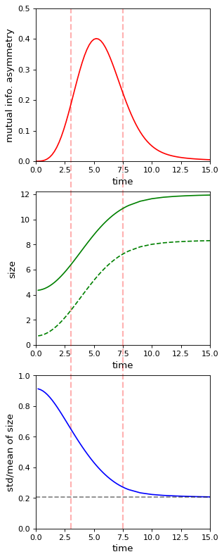
Figure 4: Operator size growth for the wormhole teleportation protocol with $N$$=$$24$, $q$$=$$8$, ${\cal J}$$=$$1$, $\beta$$=$$8$, and $\mu$$=\pm 0.2$. Top: The mutual information asymmetry as a function of time. Middle: The mean size of the thermal fermion operator $\psi_{i}^{\ell}(t)\rho^{1/2}$ (solid line) and the same quantity but subtracting off the size of $\rho^{1/2}$ (dashed line). Bottom: The standard deviation of the thermal fermion size distribution divided by the mean size (solid line); for comparison the dashed line shows $1/\sqrt{N}$.

Figure 4 shows the operator size growth over time of the thermal fermion $O_{L}^{\beta}(t)$, for the case $N$$=$$24$, $q$$=$$8$, ${\cal J}$$=$$1$, $\beta$$=$$8$. For comparison, the top plot shows the mutual information asymmetry, i.e. the difference between $I(R$$:$$T)$ resulting from performing the teleportation protocol using a negative coupling $\mu$$=-0.2$ and $I(R$$:$$T)$ resulting from using a positive coupling $\mu$$=+0.2$. The vertical dashed red line lines define the approximate range of injection times (enforcing, for simplicity, $t_{0}$$=$$t_{1}$) over which the holographic dynamics dominates the transfer of quantum information.

The solid line in the middle plot shows the mean size of a left thermal fermion, which we denote as $n[\psi_{i}^{\ell}(t)\rho^{1/2}]$; the dashed line shows the difference between this quantity and the time-independent size of the thermal factor $\rho^{1/2}_{\beta}$:

$$n[\rho^{1/2}_{\beta}]=\frac{N}{2}\left(1-G(\frac{\beta}{2})\right)$$ (39)

where $G(\frac{\beta}{2})$ is the Euclidean two-point function of that thermal fermion Qi and Streicher (2019):

$$G(\frac{\beta}{2})=2Z^{-1}_{\beta}{\rm Tr}\left({\rm e}^{-\beta H_{L}}\psi^{\ell}_{i}(\frac{\beta}{2})\psi^{\ell}_{i}(0)\right)=2\bra{I}\psi_{i}^{\ell}\rho^{1/2}_{\beta}\psi_{i}^{\ell}\rho^{1/2}_{\beta}\ket{I}$$ (40)

Note $G(\frac{\beta}{2})$ varies from near one at small $\beta$ to near zero at large $\beta$.

The middle plot shows that the operator size is growing rapidly over the range of times where the holographic teleportation is effective. In the large $N$, large $q$ limit this growth is exponential, and the exponent is called the Lyapunov exponent. In this limit one has Qi and Streicher (2019):

$$n[\psi_{i}^{\ell}(t)\rho^{1/2}_{\beta}]-n[\rho^{1/2}_{\beta}]=G(\frac{\beta}{2})\left(1+\frac{8{\cal J}^{2}}{\lambda^{2}}{\rm sinh}^{2}\frac{\lambda t}{2}\right)$$ (41)

where $\lambda$ denotes the Lyapunov exponent. This exponent has an upper bound, $\lambda\leq 2\pi/\beta$; black holes saturate this upper bound, as does the SYK model in the limit $N$$\to$$\infty$, $\beta{\cal J}$$\to$$\infty$, $N/\beta{\cal J}$$\to$$\infty$. While the growth described by eqn. 41 is exponential, for $\lambda t/2\lessapprox 1$ it reduces to a quadratic in time with the $\lambda$ dependence dropping out. This is the regime that we are in for the example of Figure 4, so it is not useful to try to extract the Lyapunov exponent directly from the operator size growth in this regime of parameters.

To study size winding, we begin by observing that, using eqns. 4, 35 and the hermiticity of the basis operators, it is straightforward to show:

$$\left(c^{r*}_{J}(t)\right)^{2}=\left(c^{\ell}_{J}(-t)\right)^{2}$$ (42)

Size winding is observed using the distributions:

$$Q^{\ell}(s)=\sum_{|J|=s}\left(c^{\ell}_{J}(t)\right)^{2}\;;\quad Q^{r}(s)=\sum_{|J|=s}\left(c^{r}_{J}(t)\right)^{2}$$ (43)

The size winding ansatz of Brown et al. (2021); Nezami et al. (2021) is:

$$Q^{\ell}(t)={\rm e}^{i\alpha s/N}r^{2},\;;\quad Q^{r}(t)={\rm e}^{-i\alpha s/N}r^{2}\quad\alpha,r\in\mathbb{R}$$ (44)

This is a strong ansatz since it assumes both a linear dependence of the phase on size, and an overall coherence involving the large number of distinct basis operators $\Gamma^{(s)\ell}_{J}$, $\Gamma^{(s)r}_{J}$ of a given size.

Notice that the phases of the individual $c_{J}$ depend on the choice of basis operators $\Gamma^{(s)}_{J}$; if we rotate the basis operators of a given size $s$ by a real orthogonal matrix $R^{(s)}_{JK}$, the $c_{J}$ change but the corresponding $Q(s)$ are basis independent:

$$\tilde{\Gamma}^{(s)}_{J}\equiv\sum_{K}\Gamma^{(s)}_{K}R_{KJ}\;;\quad\tilde{c}^{(s)}_{J}\equiv\sum_{K}c^{(s)}_{K}R_{KJ}$$

$$\sum_{J}c^{(s)}_{J}\Gamma^{(s)}_{J}=\sum_{J}\tilde{c}^{(s)}_{J}\tilde{\Gamma}^{(s)}_{J}\;;\quad\sum_{J}\left(c^{(s)}_{J}\right)^{2}=\sum_{J}\left(\tilde{c}^{(s)}_{J}\right)^{2}$$ (45)

As in Brown et al. (2021); Nezami et al. (2021), we define “perfect size winding” by the requirement $|Q(s)|/P(s)=1$ for all sizes $s$. This would require that all the individual $c_{J}$ for a given size have the same phase, which in this limit is basis-independent since an overall phase factors out in the expressions above. Since the size winding in the systems we analyze is not perfect, we confine our attention to the basis independent quantities $Q(s)$. However we use the ratio $|Q(s)|/P(s)$ as a diagnostic of the overall coherence of the size winding phenomenon.

To understand the effect of the Left-Right interaction operator exp$i\mu V$ on size winding, let’s rewrite the expression eqn. 6 for $V$ as:

$$V=\frac{i}{2}\sum_{j=0}^{N-1}\,\Gamma_{j}^{(1)\ell}\Gamma_{j}^{(1)r}$$ (46)

where we have used the size 1 basis operators $\Gamma_{j}^{(1)\ell}=\sqrt{2}\psi_{j}^{\ell}$ and $\Gamma_{j}^{(1)r}=\sqrt{2}\psi_{j}^{r}$, which obey the following commutation relations with other left basis operators:

$$\Gamma_{j}^{(1)\ell}\Gamma_{j}^{(1)r}\Gamma_{J}^{(s)\ell}=(-1)^{j\cap J}\Gamma_{J}^{(s)\ell}\Gamma_{j}^{(1)\ell}\Gamma_{j}^{(1)r}$$ (47)

Given also that $\Gamma_{j}^{(1)\ell}\Gamma_{j}^{(1)r}\ket{I}=i\ket{I}$, this implies

$$\bra{I}\Gamma_{J}^{(s)\ell}\,V\,\Gamma_{J}^{(s)\ell}\ket{I} =-\frac{1}{2}\sum_{|j\cap J|=0}+\frac{1}{2}\sum_{|j\cap J|=1}$$

$$=s-\frac{N}{2}$$ (48)

Thus $V$, up to an overall additive constant, measures the size $s$ of any basis operator, and the Left-Right interaction exp$i\mu V$ applies a size-dependent phase that corresponds to shifting $Q^{\ell}(s)$ by $2\mu s$.

What does this imply for the wormhole teleportation protocol? If at injection time $c^{\ell}_{J}(-t_{0})$ already possesses the linear size dependence of eqn. 44 with some positive slope $\alpha/N$, then applying the Left-Right interaction with $\mu\simeq-\alpha/N$ at $t=0$ can have the effect of reversing the sign of the size winding, thus coherently converting Left side size winding to Right side size winding.

The holographic description of teleportation through the wormhole with two entangled copies of the SYK model is explained in detail in Maldacena et al. (2017); Maldacena and Qi (2018); Lin et al. (2019), and the mapping between this description and size winding is discussed in Brown et al. (2021); Nezami et al. (2021). In the holographic picture an emergent spatial degree of freedom combines with time in a nearly-AdS₂ geometry; the geometry is nearly-AdS in that it includes leading effects that break conformal symmetry, consistent with the fact that the low energy correlators of the SYK model are “nearly” conformal. Gravity in such a system was first described by Jackiw and Teitelboim Jackiw (1985); Teitelboim (1983); it has no propagating degrees of freedom, but there is a gravitational mode that maps the proper time on the nearly-AdS boundary to AdS₂ time as expressed in Poincare or Rindler coordinates. The holographic dual system of JT gravity coupled to bulk matter has an approximate $SL(2,R)$ symmetry generated by $B$, $E$, and $-i[B,E]$, where

$$B=H_{R}-H_{L}\;;\quad E=H_{L}+H_{R}-\mu V-E_{0}$$ (49)

and $E_{0}$ is a constant. The boost operator $B$ annihilates our $t$$=$$0$ state, i.e., the thermofield double state $\ket{\rm tfd}$. The operator $E$, which can be considered as generating global time translations, also approximately annihilates $\ket{\rm tfd}$ for a suitable choice of $E_{0}$; we quantify this statement with examples in subsection V.5. Translations along the two bulk null directions are generated by

$$P_{\pm}=-\frac{1}{2}\left(E\pm B\right)$$ (50)

From this correspondence it was shown in Brown et al. (2021); Nezami et al. (2021) that size winding describes the momentum wavefunction of a particle traversing the emergent wormhole, where the conjugate position describes the particle location relative to the horizon.

Figure 5: Example of size winding. Left: Phase of $Q^{\ell}(s)$ as a function of the operator size $s$ for the first 10 fermions of a single instantiation of the wormhole protocol with $N$$=$$20$, $q$$=$$4$, $\beta$$=$$4$, ${\cal J}$$=$$1$, $t_{0}$$=$$2.9$, $\mu$$=$$-0.2$, using $V$ to generate the Left-Right interaction; the upper dashed black line is a linear fit to the Left size winding, weighted by the probability $P^{\ell}(s)$; the lower dashed black line is the corresponding Right size winding, and the orange dashed line is a linear fit to the actual points after applying the Left-Right interaction. Right: The mutual information asymmetry for the same parameters, fixing also $t_{1}$$=$$t_{0}$; the dashed line shows $t_{0}$$=$$2.9$.

Figure 5 (Left) shows size winding for the case $N$$=$$20$, $q$$=$$4$, $\beta$$=$$4$, ${\cal J}$$=$$1$, $t_{0}$$=$2.9, $\mu$$=$$-0.2$, using $V$ for the Left-Right interaction. The time chosen corresponds approximately to the peak in the mutual information asymmetry. We see excellent agreement with the expected linear dependence of the phase on size, and that the Left-Right interaction flips Left size winding to Right size winding, in agreement with the holographic interpretation with a traversable wormhole. The figure superimposes the phases for 10 of the 20 Majorana fermions in the model; the fact that every fermion has identical behavior is a consequence of the self-averaging of the SYK model for this value of $N$.

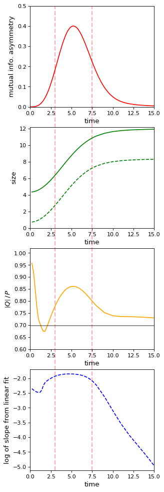
Figure 6: Size winding of the Gao-Jafferis wormhole teleportation protocol with $N$$=$$24$, $q$$=$$8$, ${\cal J}$$=$$1$, $\beta$$=$$8$, and $\mu$$=\pm 0.2$. Top: The mutual information asymmetry as a function of time. Second: The mean size of the thermal fermion operator. Third: $|Q|/P$ (orange line) averaged over size; the solid black line denotes $G(\beta)$. Bottom: The log of the fitted linear size winding slope.

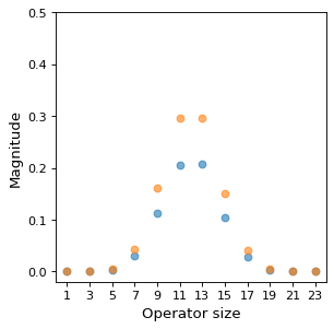
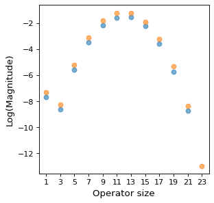
Figure 7: Distribution of the thermal fermion operator size at the scrambling time $t$$=$$15$, for the $N$$=$$24$ SYK model with $q$$=$$8$, $\cal J$$=$$1$, $\beta$$=$$8$, shown on a linear scale (left) and a log scale (right). The orange points are $P(s)$ as defined in eqn. V.1; also shown (blue points) are $|Q(s)|$ as defined in eqn. 43.

Figure 8: Distribution of the thermal fermion operator size at time $t$$=$$2.9$. Shown are $|Q^{\ell}(s)|$ (blue) and $P^{\ell}(s)$ (orange) as a function of the operator size $s$, averaged over the first 10 fermions of a single instantiation of the wormhole teleportation protocol with $N$$=$$20$, $q$$=$$4$, $\beta$$=$$4$, ${\cal J}$$=$$1$, on a linear scale (left) and a log scale (right).

V.2 Peaked-size teleportation

A universal feature of SYK scrambling dynamics is that, as the teleportation time interval is increased, the mean operator size eventually asymptotes to $N/2$. This scrambling time is roughly 15 for the example shown in Figure 4. As seen in Figure 7, at the scrambling time the operator size distribution is strongly and symmetrically peaked around $N/2$. The lower plot of Figure 4 shows that the standard deviation of the operator size distribution, in units of the mean size, starts out close to one at early times, but by the scrambling time has asymptoted to $1/\sqrt{N}$.

As observed in Schuster et al. (2022), if we choose the injection $t_{0}$ in the teleportation protocol to be greater than or equal to the scrambling time, then at $t$$=$$0$ the size of a thermal fermion for large $N$ will be strongly peaked at $N/2$. This allows the Left-Right interaction using the size operator to preserve quantum information transfer without invoking size winding.

This non-holographic many-body quantum effect, dubbed peaked-size teleportation in Schuster et al. (2022), will also be present at some level for $t_{0}$ values smaller then the scrambling time, including values where our through-the-wormhole quantum teleportation dominates. This is quantified in the long-range wormhole teleportation protocol, where the direct transmission mechanism is absent. Thus for example the red dashed line in Figure 3 represents quantum information transfer coming entirely from the “peaked-size teleportation”. In the infinite temperature limit (i.e. $\beta\to 0$) the through-the-wormhole teleportation disappears while the peaked-size teleporation remains; the size winding phases also disappear in this limit, since for $\beta$$=$$0$ the operators in Eq. V.1 are Hermitian.

Figure 8 shows the thermal fermion size distribution in an example of the Gao-Jafferis wormhole teleportation with $t_{0}$$=$$t_{1}$$=$$2.9$, approximately the choice that optimizes the holographic quantum information transfer. Note that the size distribution is not centered around $N/2$ and is more spread out than the late time example of Figure 7.

V.3 Size winding with the long-range protocol

The alert reader may at this point despair for the long-range protocol, in which $V$ has been replaced by $V^{b}$. How can we preserve the holographic size winding feature without using the size operator $V$? The answer is that $V^{b}$ is also a size operator equivalent to $V$. To see this, start with the definition of $V^{b}$ in eqn. 26 and write the commutation relations analogous to eqn. 47:

$$\Gamma_{j}^{(2)\ell}\Gamma_{j}^{(2)r}\Gamma_{J}^{(s)\ell}=(-1)^{j\cap J}\Gamma_{J}^{(s)\ell}\Gamma_{j}^{(2)\ell}\Gamma_{j}^{(2)r}$$ (51)

Then we use $\Gamma_{j}^{(2)\ell}\Gamma_{j}^{(2)r}\ket{I}=-\ket{I}$ to find:

$$\bra{I}\Gamma_{J}^{(s)\ell}\,V^{b}\,\Gamma_{J}^{(s)\ell}\ket{I} =-\sum_{|j\cap J|=0}+\sum_{|j\cap J|=1}-\sum_{|j\cap J|=2}$$

$$=s_{2}-\frac{N}{2}$$ (52)

where $s_{2}$ is the size measured by $V^{b}$. In terms of Majorana operator strings realized on qubits, it is easy to see the relation between the size $s$ measured by $V$ and the size $s_{2}$ measured by $V^{b}$: $s$ counts the number of Majoranas in the operator string, while $s_{2}$ counts the number of Majoranas in the operator string not counting pairs of Majoranas residing on the same qubit. Note that the maximum value of $s_{2}$ is $N/2$.

Figure 9 shows size winding using $V^{b}$ for the Left-Right interaction and as the size operator, for the case $N$$=$$20$, $q$$=$$4$, $\beta$$=$$4$, ${\cal J}$$=$$1$, $t_{0}$$=$$t_{1}$$=$$2.4$, $\mu$$=$$-0.2$.

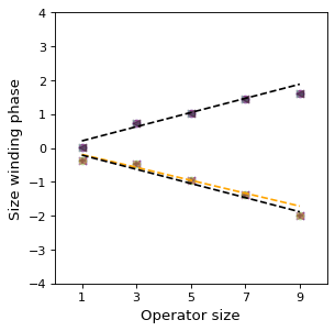
Figure 9: Example of size winding in the long-range wormhole teleportation protocol. Left: Phase of $Q^{\ell}(s)$ as a function of the operator size $s$ for the first 10 fermions of a single instantiation of the long-range wormhole protocol with $N$$=$$20$, $q$$=$$4$, $\beta$$=$$4$, ${\cal J}$$=$$1$, $t_{0}$$=$$2.4$, $\mu$$=$$-0.2$, using $V^{b}$ to generate the Left-Right interaction and as the size operator. The upper dashed black line is a linear fit to the Left size winding, weighted by the probability $P^{\ell}(s)$; the lower dashed black line is the corresponding right size winding, and the orange dashed line is a linear fit to the actual points after applying the Left-Right interaction. The x-axis is the size as measured by $V^{b}$, as defined in Eq. V.3. Right: The mutual information asymmetry for the same parameters, fixing also $t_{1}$$=$$t_{0}$; the dashed line shows $t_{0}$$=$$2.4$.

Figure 10: Size winding of the long-range wormhole teleportation protocol with $N$$=$$24$, $q$$=$$8$, ${\cal J}$$=$$1$, $\beta$$=$$8$, and $\mu$$=\pm 0.2$. Top: The mutual information asymmetry as a function of time. Second: The mean size of the thermal fermion operator. Third: $|Q|/P$ (orange line) averaged over size; the solid black line denotes $G(\beta)$. Bottom: The log of the fitted linear size winding slope.

V.4 Extracting the Lyapunov exponent from size winding

As already noted, operator size growth from scrambling in the SYK model is related to the Lyapunov exponent, but in our finite $N$ examples it is not possible to extract this exponent directly from the observed growth rate over the relevant time range. However, as observed by Nezami et al. (2021), in the large $N$, large $q$ limit of wormhole teleportation, as one approaches the scrambling time, the magnitude of the size winding slope decreases exponentially like exp$(-\lambda t)$, where $\lambda$ is again the Lyapunov exponent.

We see a corresponding behavior in our finite $N$, finite $q$ examples. This is shown for the Gao-Jafferis protocol in Figure 6, for the same cases as Figure 4: the first two plots starting from the top are the same as in Figure 4. The third plot shows the coherence diagnostic, i.e., the value of $|Q(s)|/P(s)$ averaged over size; notice that the coherence peaks in the time interval where the mutual information asymmetry peaks. The bottom plot shows the log of the magnitude of the fitted linear size winding slope; this also peaks in the time interval where the mutual information asymmetry peaks. Furthermore at later times the plot shows an exponential decline over time ranging from about 7.5 to the scrambling time 15. Figure 10 demonstrates similar behavior for the long-range wormhole teleportation protocol.

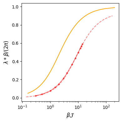
Figure 11: Lyapunov exponents. Left: The orange line is the SYK model Lyapunov exponent as a function of $\beta{\cal J}$, calculated in the large $N$, large $q$ limit Maldacena and Stanford (2016). The red points are exponents extracted from the fitted size winding slope of the SYK model with $N$$=$$26$, $q$$=$$8$, ${\cal J}$$=$$1$, fitting to an exponential over times ranging from 7.5 to 15. The dashed red line is a fit to the red points using a functional form similar to the orange line. Middle: Lyapunov exponents for different $N$. The red points are exponents extracted from the fitted size winding slope of the SYK model with $N$$=$$26$, $q$$=$$8$, ${\cal J}$$=$$1$, fitting to an exponential over times ranging from 7.5 to 15. Corresponding results are also shown for $N$$=$$24$ (blue points) and $N$$=$$22$ (green points). Right: The same as the left plot, but adding the corresponding results for size winding with sizes measured by $V^{b}$ (purple points).

Figure 11 shows the Lyapunov exponents as a function of $\beta$ as extracted from the size winding slope exponential dropoff. Here we have used the largest values of $N$ and $q$ available to us, attempting to make contact with the known analytic result for the large $N$, large $q$ limit Maldacena and Stanford (2016). In the plot we only use values of beta small enough that $\lambda t\gtrapprox 2$ over the fitted time range, to ensure that we are in the exponential regime.

The qualitative agreement with the large $N$, large $q$ result is encouraging, and resembles the large $N$, finite $q$ result obtained numerically and shown in Figure 11 of Maldacena and Stanford (2016). One would expect the agreement to worsen as we decrease $N$ and indeed this is the case, as shown in Figure 11.

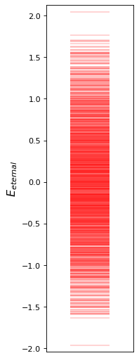
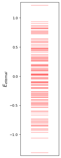
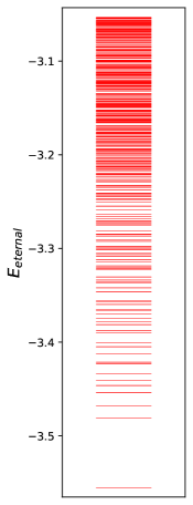
Figure 12: Spectra of the eternal traversable wormhole. Left: Using the $N$$=$$10$, $q$$=$$4$, ${\cal J}$$=$$1$ SYK model, averaged over 10 instantiations, and the interaction $V$ with $\mu$$=$$0.3$. Middle: Using the Learned17 model with $\mu$$=$$0.3$. Right Using the $N$$=$$18$, $q$$=$$4$, ${\cal J}$$=$$1$ SYK model, averaged over 10 instantiations, and the interaction $V^{b}$ with $\mu$$=$$0.3$; only the lowest 600 energy eigenstates are shown.

V.5 Eternal traversable wormhole

As discussed by Maldacena and Qi (2018), The holographic dual description can be elucidated by studying properties of the “eternal” traversable wormhole evident in the dynamics of the Hamiltonian

$$H_{\rm eternal}=H_{L}+H_{R}+\mu V$$ (53)

where here positive values of $\mu$ correspond to negative values of $\mu$ in the wormhole teleportation protocol (this is just the sign difference between applying a Left-Right interaction exp$(i\mu V)$ and performing time evolution with exp$(-i(H_{L}+H_{R}+\mu V)t)$).

The approximate $SL(2,R)$ remnant of reparametrization invariance is here related to a gap in the energy spectrum of $H_{\rm eternal}$. This gap is a robust feature evident already for $N$$=$$10$, as seen in Fig. 12. Here we also show the spectrum of our learned Hamiltonian used in the Google Sycamore experiment described in Jafferis et al. (2022). We henceforth refer to this as Learned17, since for this model $H_{\rm eternal}$ has 17 terms. In the large $N$ limit, Maldacena and Qi (2018) showed that the dependence of the energy gap on the coupling $\mu$ has two regimes: for large $\mu$ the energy gap grows linearly with $\mu$, while for small $\mu$ the dependence is related to the holographic $SL(2,R)$ symmetry. In the large $N$ limit with $q$$=$$4$, the prediction for the small $\mu$ regime is $E_{\rm gap}\propto\mu^{2/3}$. Fig. 13 shows the results of our simulation for $N$$=$$20$; the two distinct regimes are clearly visible, and a simple fit to the small $\mu$ behavior gives $E_{\rm gap}\propto\mu^{0.69}$, consistent with the large $N$ result. Similar results at finite $N$ were obtained in García-García et al. (2019).

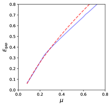
Figure 13: The energy gap of the eternal traversable wormhole as a function of $\mu$, for $N$$=$$20$, $q$$=$$4$, ${\cal J}$$=$$1$ (blue solid line). The red dashed line shows a fit of the $\mu<0.3$ portion of this result to a simple power law behavior $E_{\rm gap}=a\mu^{b}+c$, with $a,b,c$ = 1.3, 0.69, and -0.17 respectively.

As detailed in Maldacena and Qi (2018), one expects the thermofield double state $\ket{\rm tfd}$ of the wormhole teleportation protocol to approximate the ground state $\ket{\rm G}$ of $H_{\rm eternal}$. Indeed the overlap $\bra{\rm tfd}\ket{\rm G}$ approaches unity in two limits. The first limit is $\mu$ becoming large, where $\ket{\rm G}\to\ket{I}$, since as we saw in Eq. V.1, this maximally entangled state yields the minimum expectation value of the size operator $V$. Since $\ket{I}$ is also the infinite temperature limit of $\ket{\rm tfd}$, we see that $\bra{\rm tfd}\ket{\rm G}\to 1$ as $\mu\to\infty$ and $\beta\to 0$. The second limit is $\mu\to 0$, $\beta\to\infty$, since in this limit $H_{\rm eternal}\to H_{L}+H_{R}$, and large $\beta$ concentrates the support of the $\ket{\rm tfd}$ onto the SYK ground state.

In between these two limits, one can adjust $\beta$ as a function of $\mu$ to maximize the overlap $\bra{\rm tfd}\ket{\rm G}$. This leads to curves like those in Fig. 14. It is interesting to note from this figure that for the $N$$=$$10$, $q$$=$$4$, ${\cal J}$$=$$1$ model first discussed in Jafferis et al. (2022), optimizing the overlap in $\bra{\rm tfd}\ket{\rm G}$ gives a relation between $\beta$ and $\mu$ consistent with that obtained by asking for optimal mutual information transfer in the wormhole teleportation protocol. Furthermore, the Learned17 model of Jafferis et al. (2022) tracks the $\beta$ vs $\mu$ behavior of its parent SYK-based model over a large range.

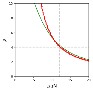
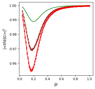
Figure 14: Left: The relation between $\beta$ and $\mu$ obtained by maximizing the overlap $\bra{\rm tfd}\ket{\rm G}$, shown for $H_{\rm eternal}$ with $N$$=$$10$, $q$$=$$4$, ${\cal J}$$=$$1$ averaged over 10 instantiations (red points), as well as the Learned17 model (green line) of Jafferis et al. (2022). The dashed lines show the values of $\mu$ (scaled by $qN$ as in Jafferis et al. (2022)), and $\beta$ that give the optimal mutual information transfer in the wormhole teleportation protocol, as described in Jafferis et al. (2022). Right: The maximal overlap of the $H_{\rm eternal}$ ground state and the thermofield double state, as a function of $\mu$, with $H_{L}$,$H_{R}$ taken from the $N$$=$$10$, $q$$=$$4$, ${\cal J}$$=$$1$ SYK model averaged over 10 instantiations (red points), the $N$$=$$8$, $q$$=$$4$, ${\cal J}$$=$$1$ SYK model averaged over 10 instantiations (brown points), and the Learned17 model of Jafferis et al. (2022) (green line).

If we now fix the relation between $\beta$ and $\mu$ by the criterion of maximizing the overlap of the $H_{\rm eternal}$ ground state and the thermofield double state, we can plot the maximal overlap as a function of $\mu$, as shown in Fig. 14 with $H_{L}$,$H_{R}$ taken from three example Hamiltonians: the $N$$=$$10$, $q$$=$$4$, ${\cal J}$$=$$1$ SYK model, the $N$$=$$8$, $q$$=$$4$, ${\cal J}$$=$$1$ SYK model, and the Learned17 model of Jafferis et al. (2022). In all cases (as previously noted for several examples in Maldacena and Qi (2018)) the overlap is close to unity over the entire range.

In the wormhole teleportation protocol, the Left-Right interaction exp$(i\mu V)$ is applied at $t$$=$$0$ when the state of the system, by construction, is close to $\ket{\rm tfd}$. It is thus interesting to construct a measure of how well $\ket{\rm tfd}$ respects the part of the approximate $SL(2,R)$ symmetry that generates global time translations. A reasonable figure of merit is

$$\frac{\bra{\rm tfd}(H_{\rm eternal}-E_{0})\ket{\rm tfd}}{|E_{0}|}$$ (54)

where $E_{0}$ is the energy of the true ground state $\ket{\rm G}$ of $H_{\rm eternal}$. When this quantity is small, the expectation values of all three $SL(2,R)$ generators in the thermofield double state either vanish or are small in natural units.

We plot this quantity in Fig. 15 (Left) for several examples of the Gao-Jafferis protocol. Recall that $\mu$$\simeq$$0.3$ optimizes the mutual information transfer in the wormhole teleportation protocol for both the $N$$=$$10$ and the Learned17 models, as discussed in Jafferis et al. (2022). In the figure we show for comparison $E_{\rm gap}/|E_{0}|$, i.e., the energy gap in units of the magnitude of the ground state energy. Notice that in all four examples the figure of merit is both numerically small and smaller than the rescaled gap energy; this can be taken as an indication that the $SL(2,R)$ symmetry is indeed approximately respected.

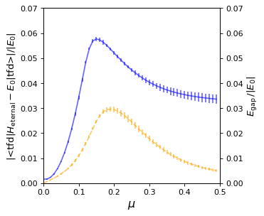
Figure 15: $SL(2,R)$ symmetry. Left: The figure of merit defined in Eq. 54, as a function of $\mu$, for the Gao-Jafferis wormhole teleportation protocol with $H_{L}$,$H_{R}$ taken from the $q$$=$$4$, ${\cal J}$$=$$1$ SYK model averaged over 10 instantiations with $N$$=$$12$ (blue solid), $N$$=$$10$ (red solid), $N$$=$$8$ averaged over 40 instantiations (brown solid), and the Learned17 model of Jafferis et al. (2022) (green solid). Shown on the same scale, with the same color coding but dashed lines, is the corresponding value of $E_{\rm gap}$, also in units of $|E_{0}|$. Right The same figure of merit (blue points) for the long-range wormhole teleportation protocol, with $H_{L}$,$H_{R}$ taken from the $N$$=$$18$, $q$$=$$4$, ${\cal J}$$=$$1$ SYK model averaged over 20 instantiations. Shown on the same scale (orange dashed lines) is the corresponding value of $E_{\rm gap}$ in units of $|E_{0}|$. In all cases $\beta$ is set to the value that minimizes $\bra{\rm tfd}(H_{\rm eternal}$$-$$E_{0})\ket{\rm tfd}/|E_{0}|$.

V.6 Modified Eternal Hamiltonian

We perform a similar analysis now for a modified version of the Hamiltonian in Eq. 53, where we replace the interaction operator $V$ with $V^{b}$:

$$H^{b}_{\rm eternal}=H_{L}+H_{R}+\mu V^{b}$$ (55)

It is useful at this point to identify some discrete symmetries respected by these two eternal Hamiltonians. As already discussed by García-García et al. (2019), the original eternal Hamiltonian of Eq. 53 commutes with the operator $Q$ defined by

$$Q\equiv{\rm e}^{i\pi V/2}$$ (56)

The operator $Q$ has eigenvalues: $\pm 1$, $\pm i$. The square of $Q$ is the overall parity operator $\Gamma^{5}$:

$$Q^{2}=\Gamma^{5}=\Gamma^{5}_{R}\cdot\Gamma^{5}_{L}\;;\quad{\rm where:}\quad\Gamma^{5}_{L}=\prod_{j=0}^{N-1}\Gamma^{(1)\ell}_{j}\;;\quad\Gamma^{5}_{R}=\prod_{j=0}^{N-1}\Gamma^{(1)r}_{j}$$ (57)

The Left and Right side parity operators $\Gamma^{5}_{L}$ and $\Gamma^{5}_{R}$ commute with each other and have eigenvalues $q_{L},q_{R}$$=$$\pm 1$, but they do not commute with $H_{\rm eternal}$. Obviously $\Gamma^{5}$ does commutes with the eternal Hamiltonian and also has eigenvalues $\pm 1$.

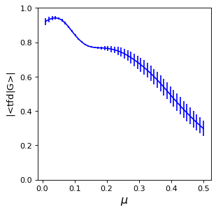
Figure 16: Left: The relation between $\beta$ and $\mu$ obtained by maximizing the overlap $\bra{\rm tfd}\ket{\rm G}$, shown for $H_{\rm eternal}$$=$$H_{L}$$+$$H_{R}$$+$$\mu V^{b}$ with $q$$=$$4$, ${\cal J}$$=$$1$ and $N$$=$$18$ averaged over 20 instantiations (green points), as well as $N$$=$$20$ averaged over 10 instantiations (red points), The dashed lines show the approximate values of $\mu$ and $\beta$ that give the optimal mutual information transfer in the long-range wormhole teleportation protocol. Right: The maximal overlap of the modified $H_{\rm eternal}$ ground state and the thermofield double state, as a function of $\mu$, with $H_{L}$,$H_{R}$ taken from the $N$$=$$18$, $q$$=$$4$, ${\cal J}$$=$$1$ SYK model averaged over 20 instantiations.

Our modified eternal Hamiltonian $H^{b}_{\rm eternal}$ has additional discrete symmetries. It commutes with $Q$, and also commutes with the Left/Right parity operators $\Gamma^{5}_{L}$, and $\Gamma^{5}_{R}$ individually, in addition to the total parity operator $\Gamma^{5}$.

From Eqs. 56 and 57 one can easily show that the discrete symmetry operators $Q$ and $\Gamma^{5}_{L}$ commute with each other when $N$$=$$0$ (mod 4), but anti-commute with each other when $N$$=$$2$ (mod 4).

Figure 12 (Right) shows the 600 lowest energy eigenvalues of $H^{b}_{\rm eternal}$ using the $N$$=$$18$, $q$$=$$4$, ${\cal J}$$=$$1$ SYK model, averaged over 10 instantiations, and the interaction $V^{b}$ with $\mu$$=$$0.3$. Since $N$$=$$18$$=$$2$ (mod 4), $Q$ acting on an eigenstate of $\Gamma^{5}_{L}$, or vice versa, gives a new state with the same energy eigenvalue. Thus in this spectrum all of the energy eigenstates are doubly degenerate. The ground state pair has $q_{Q}$$=$$\pm i$ with a suitable choice of basis, and has $q_{L}$$=$$\pm 1$ in a different suitable choice of basis. We see in the figure that an energy gap is evident; more generally we find that the spectra of $H^{b}_{\rm eternal}$ and $H_{\rm eternal}$ are qualitatively similar.

Figure 16 (Left) plots the value of $\beta$ as a function of $\mu$ that maximizes the overlap $\bra{\rm tfd}\ket{\rm G}$, where $\ket{\rm G}$ now denotes the ground state of the modified eternal Hamiltonian Eq. 55. As for the original eternal Hamiltonian Eq. 53, optimizing this overlap gives a relation between $\beta$ and $\mu$ consistent with that obtained by asking for optimal mutual information transfer in the wormhole teleportation protocol. In Figure 16 (Right) we see that the overlap $|\bra{\rm tfd}\ket{\rm G}|$ is fairly large in the relevant range of $\mu$, but significantly smaller than we had found in Figure 14 for the original eternal Hamiltonian.

Figure 15 (Right) shows the figure of merit defined in Eq. 54 for the long-range wormhole teleportation protocol, as a function of $\mu$ for the modified eternal Hamiltonian $H^{b}_{\rm eternal}$ with $N$$=$$18$, $q$$=$$4$, ${\cal J}$$=$$1$. Shown on the same scale is the corresponding value of the energy gap in units of $|E_{0}|$. Comparing to the results for $H_{\rm eternal}$ shown in Figure 15 (Left), note that for $H^{b}_{\rm eternal}$ the figure of merit is numerically quite small, but not smaller than the rescaled energy gap.

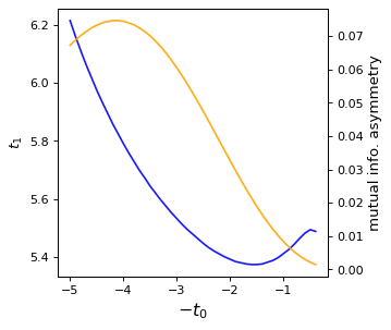
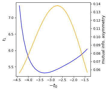
Figure 17: Causal time ordering of long-range wormhole teleportation. Left: $N$$=$$24$, $q$$=$$8$, ${\cal J}$$=$$1$, $\beta$$=$$20$. The Left-Right interaction using $V^{b}$ is applied at time $t$$=$$0$, with coupling strength $\mu$$=$$-0.18$. The blue line shows the extraction time $t_{1}$ as a function of insertion time $t_{0}$, as determined by maximizing the resulting mutual information asymmetry. The orange line shows the corresponding mutual information asymmetry. Right: $N$$=$$26$, $q$$=$$8$, ${\cal J}$$=$$1$, $\beta$$=$$16$. The Left-Right interaction using $V^{b}$ is applied twice, with coupling strength $\mu$$=$$-0.11$, at times $t$$=$$\pm 1.5$.

VI Causal time ordering

Figure 17 illustrates two examples of the causal time ordering of long-range wormhole teleportation. For large $t_{0}$,$t_{1}$ (left side of each plot), the “peaked-size teleporation” dominates, and the time ordering is “first in, last out”, as one would expect for any many-body mechanism based on scrambling followed by unscrambling. For times when the holographic wormhole teleportation dominates (right side of each plot), we see instead the causal time ordering “first in, first out”, that one would expect from traversing through a wormhole.

The example in the left plot uses $N$$=$$24$, $q$$=$$8$, ${\cal J}$$=$$1$, $\beta$$=$$20$, and the Left-Right interaction using $V^{b}$ is applied at time $t$$=$$0$, with coupling strength $\mu$$=$$-0.18$. The blue line shows the extraction time $t_{1}$ as a function of insertion time $t_{0}$, as determined by maximizing the resulting mutual information asymmetry. The orange line shows the corresponding mutual information asymmetry. While the causal time ordering is evident at early times, at later times the opposite time ordering, which arises from “peaked-size teleportation” and has steeper intrinsic slope, quickly dominates. Since some amount of “peaked-size teleportation” is always present during the period when the holographic wormhole teleportation is operative, it is non-trivial to predict over what time interval, if any, the causal time ordering dominates.

The example in the right plot uses $N$$=$$26$, $q$$=$$8$, ${\cal J}$$=$$1$, $\beta$$=$$16$. In this example, instead of applying the Left-Right interaction using $V^{b}$ at $t$$=$$0$, with coupling strength $\mu$$=$$-0.18$, we instead apply the Left-Right interaction twice, with a weaker coupling strength $\mu$$=$$-0.11$, at times $t$$=$$\pm 1.5$. Applying the Left-Right interaction in multiple time slices disfavors the “peaked-size teleportation” in favor of the holographic wormhole mechanism, increasing the time interval over which the causal time ordering is apparent. This is a general feature that applies also to the original Gao-Jafferis protocol, as noted in Jafferis et al. (2022).

VII Measurement, multipartite entanglement, and a classical channel

In order to implement a classical channel for long-range wormhole teleportation, two modifications of the protocol are required:

• At time $t=0$, instead of applying the Left-Right interaction operator exp$(i\mu V^{b})$, Alice measures the $2^{N/2}$ Left side qubits and communicates the result to Bob through a classical channel.

• Bob applies the Right side operator

  $$V^{cc}\equiv{\rm exp}\left(i\mu\sum_{j=0}^{N/2-1}\,s_{j}\,Z_{j+N/2}\right)$$ (58)

  where $s_{j}$ are the Pauli $Z$ eigenvalues $\pm 1$ of the measured left qubits.

• At time $t=t_{1}$, Bob swaps the first right qubit with the qubit $T$.

• If the measured parity $\Gamma^{5}_{\ell}$ was -1, Bob also applies a Pauli $Z$ gate to the qubit $T$.

To understand the role of multipartite entanglement in this protocol, we start with the simple case of the protocol with $t_{0}$$=$$t_{1}$$=$$\beta$$=$0. Since in this case there is no scrambling, we only need to consider the 5-qubit system $RQ\ell rT$, where $\ell$,$r$ refer to the first Left and first Right qubits, respectively. The $\beta$$=$$0$ initial state is

$$\frac{1}{\sqrt{2}}\left(\ket{00}_{RQ}+\ket{11}_{RQ}\right)\otimes\frac{1}{\sqrt{2}}\left(\ket{01}_{\ell r}+i\ket{10}_{\ell r}\right)\otimes\ket{0}$$ (59)

After applying the long-range protocol, the final state of the five qubits $RQ\ell rT$ is:

$$\frac{1}{2}\left({\rm e}^{-i\mu}\ket{00001}+i{\rm e}^{i\mu}\ket{01000}-{\rm e}^{i\mu}\ket{10101}+i{\rm e}^{-i\mu}\ket{11100}\right)$$ (60)

For the moment we consider the quantum channel with no measurement of the Left qubit $\ell$. Then it is easy to show that

$$I(R:T)=0\;;\quad I(R:\ell)={\rm log}_{2}\left(3-{\rm cos}(4\mu)\right)\;;\quad I(R:\ell T)=2$$ (61)

$${\rm tr}\left(\rho_{R\ell}^{2}\right)=\frac{1}{2}+2\,{\rm cos}^{2}\mu\,{\rm sin}^{2}\mu\qquad\qquad\qquad\qquad\qquad\qquad\qquad\quad$$

We see that there is no quantum information shared bilaterally between qubits $R$ and $T$, as expected. However for almost all values of the coupling $\mu$ there is tripartite mutual information $I(R$$:$$\ell$$:$$T)$ shared between qubits $R$, $\ell$, and $T$. This is computed as

$$I(R:\ell:T)=I(R:T)+I(R:\ell)-I(R:\ell T)=-2+{\rm log}_{2}\left(3-{\rm cos}(4\mu)\right)$$ (62)

Thus, for example, for $\mu$$=$0 we get $I(R$$:$$T)$$=$$0$, $I(R$$:$$\ell)$$=$$1$, $I(R$$:$$\ell T)$$=$$2$, and thus $I(R$$:$$\ell$$:$$T)$$=$$-1$, the minimum (i.e. most negative) possible value. In this example the 3-qubit system $R\ell T$ in the final state is sharing one qubit worth of quantum information, with part of it shared bilaterally between $R$ and $\ell$, no information shared bilaterally between $R$ and $T$, and the rest shared non-locally.

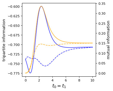
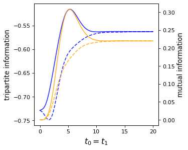
Figure 18: Multipartite quantum information sharing in the long-range wormhole teleportation protocol. Left: Using $N$$=$$24$, $q$$=$$4$, ${\cal J}$$=$$1$, $\beta$$=$$4$, and $|\mu|$$=$0.2, for a single instantiation of the SYK Hamiltonian. The blue solid/dashed lines show the tripartite information $I(R$$:$$L$$:$$T)$, where $L$ refers collectively to the 12 Left side qubits, as a function of $t_{0}$$=$$t_{1}$, for $\mu$ negative/positive. For comparison, the orange solid/dashed lines show the mutual information $I(R$$:$$T)$ for $\mu$ negative/positive. Right: Same thing for $N$$=$$24$, $q$$=$$8$, ${\cal J}$$=$$1$, $\beta$$=$$8$, and $|\mu|$$=$0.2,

Mutltipartite quantum information is a characteristic feature of scrambled systems Hosur et al. (2016), as we will see, but in this simple example there was no scrambling. Similarly holographic systems are known Hayden et al. (2013) generally to exhibit negative (or vanishing) tripartite information,i.e. they are “superextensive”, but in this simple example holography is not relevant. It is also worth observing, as noted in Hosur et al. (2016), that tripartite quantum information should really be regarded as a possible result of 4-body entanglement; in our example this is the statement that the initial state entanglement of qubits $\ell$ and $r$ is important.

To conclude our simple example consider the case $\mu$$=$$\pi/4$; now we get $I(R$$:$$\ell)$$=$$2$ and ${\rm tr}(\rho_{R\ell}^{2})$$=$$1$, so the qubits $R$ and $\ell$ are sharing all of their quantum information bilaterally, and the tripartite information $I(R$$:$$\ell$$:$$T)$ vanishes.

Figure 18 shows $I(R$$:$$L$$:$$T)$, where $L$ refers collectively to all the Left side qubits, as a function of $t_{0}$$=$$t_{1}$, for the long-range wormhole teleportation protocol with $N$$=$$24$, ${\cal J}$$=$$1$, $|\mu|$$=$$0.2$, and either $q$$=$$4$, $\beta$$=$$4$ (Left) or $q$$=$$8$, $\beta$$=$$8$ (Right). We see that $I(R$$:$$L$$:$$T)$ is negative for all values of $t_{0}$, as expected. The tripartite information as a function of $t_{0}$$=$$t_{1}$ tracks the mutual information $I(R$$:$$T)$ rather closely, and in the first example has an even more pronounced asymmetry between negative and positive values of $\mu$.

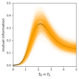
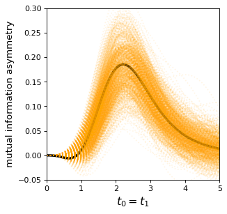
Figure 19: The effect of measuring the Left side qubits upon the end state mutual information of qubits $R$ and $T$ in the long-range wormhole teleportation protocol. The figures show the mutual information as a function of $t_{0}$$=$$t_{1}$ and the mutual information asymmetry between negative/positive values of $\mu$, for $N$$=$$20$, $q$$=$$4$, ${\cal J}$$=$$1$, $\beta$$=$$4$, and $|\mu|$$=$0.25, for a single instantiation of the SYK Hamiltonian. The black line in each figure denotes the result without measurement, while the orange dotted lines show results for all of the 1024 possible measurement outcomes.

The fact that the qubits $R$ and $T$ generally have multipartite entanglement with the Left side SYK qubits has a significant effect on the results of the classical channel long-range protocol. When the Left qubits are measured, this multipartite entanglement collapses down to bilateral entanglement between $R$ and $T$. The final value of $I(R$$:$$T)$ in general depends on the measurement outcome of the Left side qubits, and may be either larger or smaller than the value in the quantum channel protocol with no measurement.

Figure 19 shows the effect of measuring the Left side qubits upon the final state mutual information of qubits $R$ and $T$ in the long-range wormhole teleportation protocol. Here we compare, for the case $N$$=$$20$, $q$$=$$4$, ${\cal J}$$=$$1$, $\beta$$=$$4$, $|\mu|$$=$0.25, the mutual information $I(R$$:$$T)$ using either no measurement of the Left side qubits, or considering all 1024 possible measurement outcomes. We see that the value of the mutual information asymmetry does indeed depend significantly on the measurement outcome, and may be either larger or smaller.

The holographic interpretation of the traversable wormhole in the case of long-range wormhole teleportation with a classical channel was already discussed in Nezami et al. (2021), and can be extracted from the related work of Kourkoulou and Maldacena (2017) and Antonini et al. (2023).

VIII Outlook

We demonstrate a viable finite-$N$ long-range wormhole teleportation protocol, using a classical channel, and exhibit its main properties via classical computer simulation. Here we discuss the possibility of performing long-range wormhole teleportation on quantum hardware.

A quantum hardware implementation of the Gao-Jafferis protocol was reported in Jafferis et al. (2022). That experiment relied on two key enabling features: a performant quantum processor (Google Sycamore) and the use of the Learned17 model. The latter was developed starting from a model based on a single instantiation of $N$$=$$10$, $q$$=$$4$ SYK, with 430 operators total to describe $H_{L}$, $H_{R}$, and $V$. The learning procedure used gradient descent with L1 regularization and a loss function attempting to preserve a mutual information curve similar to Figure 1, and produced a learned model with 5$+$5$+$7$=$17 operators total to describe $H_{L}$, $H_{R}$, and $V$. We checked that, although it does not have single-sided late time thermalization Kobrin et al. (2023), the learned model exhibits the holographic features of wormhole teleportation, including size winding, causal time ordering, and the approximate SL(2,R) symmetry, as shown here and in Jafferis et al. (2022, 2023). These are non-trivial checks since the gradient descent loss function makes no reference to any of these features. Note also that the learning procedure is completely distinct from other procedures introduced in the literature to produce simplified versions of the SYK model, such as random sparsification Xu et al. (2020) and commuting models (see Appendix B and Gao (2023)).

Because of the difference between $V$ and $V^{b}$ as size operators (compare Eqs. V.1 and V.3) we have seen that in some respects $N$$=$$10$ Gao-Jafferis wormhole teleportation is similar to $N$$=$$20$ long-range wormhole teleportation. Thus learning or some other sparsification procedure will certainly be required to implement the long-range protocol even in the quantum channel.

Even more challenging is the prospect of performing long-range wormhole teleportation with the classical channel, thus transferring quantum information between two entangled systems that are, say, 100 km apart. Quantum teleportation systems at the 100 km scale over optical fiber already exist for the conventional Alice-Bob protocol Valivarthi et al. (2020). Long-range wormhole teleportation will require the ability, in addition, to prepare highly entangled states of many qubits in the optical domain. Performing the time evolution scrambling will require suitable quantum processors, either digital or analog Shackleton et al. (2023); Uhrich et al. (2023).

Appendix A Computation of the $t_{0}$$=$$t_{1}$$=$$\beta$$=$$\mathrm{𝟎}$ reduced density matrix for RT

The computation of the $t$$=$$0$, $\beta$$=$$0$ reduced density matrix for the reference and readout qubits $RT$ is straightforward using the following identities:

$$\chi_{\ell}^{\dagger}\chi_{\ell} =\frac{1}{2}(1+\Gamma_{0}^{(2)\ell})\;;\quad\chi_{\ell}\chi_{\ell}^{\dagger}=\frac{1}{2}(1-\Gamma_{0}^{(2)\ell})$$

$$\chi_{r}^{\dagger}\chi_{r} =\frac{1}{2}(1+\Gamma_{0}^{(2)r})\;;\quad\chi_{r}\chi_{r}^{\dagger}=\frac{1}{2}(1-\Gamma_{0}^{(2)r})$$

$$\Gamma_{0}^{(2)r}|I\rangle =-\Gamma_{0}^{(2)\ell}|I\rangle\;;\quad\quad\,\Gamma_{0}^{(2)r}\Gamma_{0}^{(2)\ell}|I\rangle=-|I\rangle$$

$$\Gamma_{0}^{(2)r}\chi_{\ell}|I\rangle =-\chi_{\ell}|I\rangle\;;\quad\quad\;\Gamma_{0}^{(2)r}\chi_{\ell}^{\dagger}|I\rangle=\chi_{\ell}^{\dagger}|I\rangle$$ (63)

$$\psi_{0}^{r}\Gamma_{0}^{(2)\ell}|I\rangle =\psi_{1}^{\ell}|I\rangle\;;\quad\quad\quad\psi_{1}^{r}\Gamma_{0}^{(2)\ell}|I\rangle=-\psi_{0}^{\ell}|I\rangle$$

$$\Gamma_{0}^{(2)r}\psi_{0}^{\ell}|I\rangle =-i\psi_{1}^{\ell}|I\rangle\;;\quad\quad\Gamma_{0}^{(2)r}\psi_{1}^{\ell}|I\rangle=i\psi_{0}^{\ell}|I\rangle$$

We also need to introduce the notation:

$$V_{01}=i\left(\psi_{0}^{\ell}\psi_{0}^{r}+\psi_{1}^{\ell}\psi_{1}^{r}\right)\;;\quad V_{0}=i\left(\psi_{0}^{\ell}\psi_{0}^{r}\right)\;;\quad V_{1}=i\left(\psi_{1}^{\ell}\psi_{1}^{r}\right)$$

and use the identities:

$$\{V_{01},\Gamma_{0}^{(2)\ell}\} =0\;;\quad\quad\quad\quad\{V_{01},\Gamma_{0}^{(2)r}\}=0$$

$$V_{01}\chi_{\ell}|I\rangle =0\;;\quad\quad\quad\quad V_{01}\chi_{\ell}^{\dagger}|I\rangle=0$$

$$V_{0}\chi_{\ell} =-\chi_{\ell}^{\dagger}V_{0}\;;\quad\quad V_{0}\chi_{\ell}^{\dagger}=-\chi_{\ell}V_{0}$$ (64)

$$V_{1}\chi_{\ell} =\chi_{\ell}^{\dagger}V_{0}\;;\quad\quad\quad V_{1}\chi_{\ell}^{\dagger}=\chi_{\ell}V_{0}$$

which imply:

$${\rm e}^{-i\mu V_{01}}\Gamma_{0}^{(2)r}\,{\rm e}^{i\mu V_{01}} ={\rm e}^{-2i\mu V_{01}}\Gamma_{0}^{(2)r}\;;\quad{\rm e}^{-2i\mu V_{01}}\Gamma_{0}^{(2)\ell}=\Gamma_{0}^{(2)\ell}\,{\rm e}^{2i\mu V_{01}}$$

$${\rm e}^{-2i\mu V_{01}}|I\rangle ={\rm e}^{2i\mu}|I\rangle\;;\quad{\rm e}^{2i\mu V_{01}}|I\rangle={\rm e}^{-2i\mu}|I\rangle$$ (65)

$${\rm e}^{-2i\mu V_{0}}\chi_{\ell}|I\rangle =-i\,{\rm sin}\mu|I\rangle\;;\quad{\rm e}^{-2i\mu V_{1}}\chi_{\ell}|I\rangle=-i\,{\rm sin}\mu|I\rangle$$

Thus for example:

$$\rho_{11} =\left\langle\chi_{\ell}\chi_{\ell}^{\dagger}\,{\rm e}^{-i\mu V}\chi_{r}\chi_{r}^{\dagger}\,{\rm e}^{i\mu V}\chi_{\ell}\chi_{\ell}^{\dagger}\right\rangle+\left\langle\chi_{\ell}^{\dagger}\,{\rm e}^{-i\mu V}\chi_{r}\chi_{r}^{\dagger}\,{\rm e}^{i\mu V}\chi_{\ell}\right\rangle$$

$$=\left\langle\frac{1}{2}(1-\Gamma_{0}^{(2)\ell})\frac{1}{2}\left(1-{\rm e}^{-2i\mu V_{01}}\Gamma_{0}^{(2)r}\right)\frac{1}{2}(1-\Gamma_{0}^{(2)\ell})\right\rangle+\left\langle\chi_{\ell}^{\dagger}\frac{1}{2}\left(1-{\rm e}^{-2i\mu V_{01}}\Gamma_{0}^{(2)r}\right)\chi_{\ell}\right\rangle$$

$$=\frac{1}{8}\left\langle(1-\Gamma_{0}^{(2)\ell})\left(1-{\rm e}^{-2i\mu V_{01}}\right)(1-\Gamma_{0}^{(2)\ell})\right\rangle+\frac{1}{2}\left\langle\chi_{\ell}^{\dagger}\left(1-{\rm e}^{-2i\mu V_{01}}\right)\chi_{\ell}\right\rangle$$

$$=\frac{1}{8}\left\langle\left(1-{\rm e}^{-2i\mu V_{01}}\right)\right\rangle+\frac{1}{8}\left\langle\Gamma_{0}^{(2)\ell}\left(1-{\rm e}^{-2i\mu V_{01}}\right)\Gamma_{0}^{(2)\ell}\right\rangle+\left\langle\chi_{\ell}^{\dagger}\chi_{\ell}\right\rangle$$ (66)

$$=\frac{1}{8}\left(1-{\rm e}^{2i\mu}+1-{\rm e}^{-2i\mu}\right)+\frac{1}{2}$$

$$=\frac{1}{2}(1+{\rm sin}^{2}\mu)$$

another example:

$$\rho_{14} =\left\langle\chi_{\ell}\,{\rm e}^{-i\mu V}\chi_{r}^{\dagger}\,{\rm e}^{i\mu V}\chi_{\ell}\chi_{\ell}^{\dagger}\right\rangle+\left\langle\chi_{\ell}^{\dagger}\chi_{\ell}\,{\rm e}^{-i\mu V}\chi_{r}^{\dagger}\,{\rm e}^{i\mu V}\chi_{\ell}\right\rangle$$

$$=\frac{1}{4}\left\langle(\psi_{0}^{\ell}+i\psi_{i}^{\ell})\left({\rm e}^{-2i\mu V_{0}}\psi_{0}^{r}-i\,{\rm e}^{-21\mu V_{1}}\psi_{1}^{r}\right)(1-\Gamma_{0}^{(2)\ell})\right\rangle$$

$$+\frac{1}{4}\left\langle(1+\Gamma_{0}^{(2)\ell})\left({\rm e}^{-2i\mu V_{0}}\psi_{0}^{r}-i\,{\rm e}^{-21\mu V_{1}}\psi_{1}^{r}\right)(\psi_{0}^{\ell}+i\psi_{i}^{\ell})\right\rangle$$ (67)

$$=\frac{i}{2}\left\langle\chi_{\ell}\left({\rm e}^{-2i\mu V_{0}}-{\rm e}^{-2i\mu V_{1}}\right)\chi_{\ell}\right\rangle-\frac{i}{8}\left\langle(1+\Gamma_{0}^{(2)\ell})\left({\rm e}^{-2i\mu V_{0}}+{\rm e}^{-2i\mu V_{1}}\right)(1-\Gamma_{0}^{(2)\ell})\right\rangle$$

$$=\frac{i}{2}\left\langle\chi_{\ell}\chi_{\ell}^{\dagger}\left(i\,{\rm sin}(2\mu V_{0})+i\,{\rm sin}(2\mu V_{1})\right)\right\rangle$$

$$\quad-\frac{i}{8}\left\langle\left({\rm e}^{-2i\mu V_{0}}+{\rm e}^{-2i\mu V_{1}}\right)\right\rangle-\frac{i}{8}\left\langle\Gamma_{0}^{(2)\ell}\left({\rm e}^{-2i\mu V_{0}}+{\rm e}^{-2i\mu V_{1}}\right)\Gamma_{0}^{(2)\ell}\right\rangle$$

$$={\rm sin}\mu$$

The final result for the $t$$=$$0$, $\beta$$=$$0$ reduced density matrix is shown is eqn. 15.

Appendix B Comparison with Gao’s commuting models

Here we make some comparisons with the non-holographic commuting models recently introduced and studied by Ping Gao Gao (2023). The purpose is to exhibit to what extent these models can be distinguished in terms of the properties of Gao-Jafferis teleportation. For simplicity we will refer to the models of Gao (2023) as “PG commuting models”, and the models of Jafferis et al. (2022) as “SYK-based models”.

Gao-Jafferis wormhole teleportation is based on SYK couplings ${\cal J}_{ijkl}$ drawn from a random Gaussian ensemble with mean zero and variance as given in Eq. 2. For $q$$=$$4$ there are ${\cal O}(N^{3})$ terms in the SYK Hamiltonian, while we scale the variance by ${\cal O}(N^{-3})$.

The PG commuting models of Gao (2023) are defined from a Hamiltonian

$$H_{L}=\sum_{(i,j)}{\cal J}_{ij}X^{\ell}_{i}X^{\ell}_{j}$$ (68)

where

$$X^{\ell}_{i}=\psi^{\ell}_{2i-2}\psi^{\ell}_{2i-1}\quad;\quad i=1,\ldots,N/2$$ (69)

and the sum in the Hamiltonian is over all the distinct tuples from choosing 2 distinct $X_{i}$ operators from $N/2$ possibilities. The couplings ${\cal J}_{ij}$ are drawn from a random Gaussian ensemble with mean zero and variance taken to be

$$\langle({\cal J}_{ij})^{2}\rangle=\frac{2^{q-1}(q/2-1)!(N/2-q/2)!}{(N/2-1)!}{\cal J}^{2}$$ (70)

with ${\cal J}$ an overall fixed constant. Note that for $q=4$ there are only ${\cal O}(N)$ terms in the commuting Hamiltonian, while we scale the variance by ${\cal O}(N^{-1})$.

Taking $\cal{J}$ =1 in both cases, the variance of the ensemble used for the PG commuting models is ${\cal O}(N^{2})$ larger than the variance of the ensemble used to define the corresponding SYK Hamiltonian. This very large ratio of variances, numerically $\gtrsim 100$ in the examples we consider, means that single instantiations of the PG commuting models are never even a rough approximation to the ensemble averages, and there is no sign of self-averaging in the PG commuting models even taking the largest $N$ values, $N\sim 20$$-$$30$, for which we can perform the simulation of the corresponding SYK-based models.

B.1 2-pt correlator of PG commuting models

In Gao (2023) the Euclidean 2-pt correlator for Left majoranas of the PG commuting models is defined as (compare to our Eq. 40):

$$G_{j}(\tau)=2Z^{-1}_{\beta}\,\bra{I}{\rm e}^{-\beta H_{L}}\psi^{\ell}_{j}(\tau)\psi^{\ell}_{j}(0)\ket{I}\;;\quad\psi^{\ell}_{j}(\tau)={\rm e}^{\tau H_{L}}\psi^{\ell}_{j}{\rm e}^{-\tau H_{L}}$$ (71)

where the Majorana index $j$ is not summed over. In Gao (2023) a closed form expression for the ensemble average of this correlator is derived in the approximation that the ensemble average of the numerator is performed separately from the ensemble average of the partition function $Z$ that appears in the denominator. The closed form expression is:

$$\overline{G_{j}(\tau)}={\rm exp}\left(-{\cal J}^{2}\tau(\beta-\tau)\right)$$ (72)

The same approximation is used in Gao (2023) to compute the OTOCs considered in the next section.

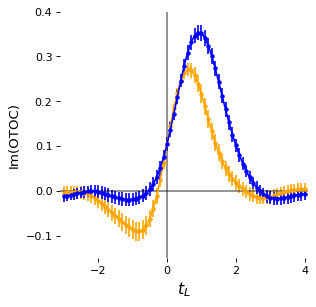
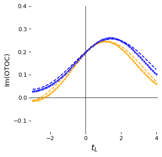
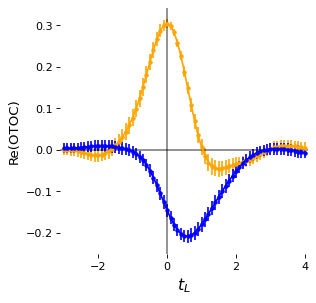
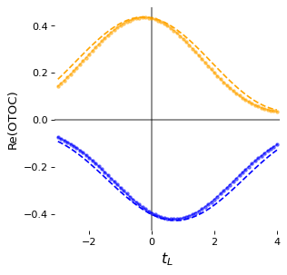
Figure 20: Comparison of $N$$=$$10$ PG commuting models (left) and SYK models (right) using a direct ensemble averaging of 100 instantiations of the finite $N$ OTOC, taking $\beta=1$, $\mu=\pm 0.139\pi$, and fixing $t_{R}=-0.720$. Shown is $-$sgn$(\mu)\,H_{i\mu}(t_{L},t_{R})$ as a function of $t_{L}$, for positive $\mu$ (blue points) and negative $\mu$ (orange points). The upper plots show the imaginary parts, and the lower plots the real parts. Also shown in the right plots are results (dashed lines) for the Learned17 SYK-based model introduced in Jafferis et al. (2022).

B.2 OTOCs

The fast scrambling behavior of the SYK model can be exhibited in a variety of out-of-time-order 4-point correlators (OTOCs). The analysis in Gao (2023) (see eqn 4.1 in that paper) uses the following OTOC in an attempt to connect to the properties of wormhole teleportation:

$$C(t_{L},t_{R})\equiv\langle{\rm tfd}|\{{\rm e}^{i\mu V}\psi^{\ell}_{j}(t_{L}){\rm e}^{-i\mu V},\psi^{r}_{j}(t_{R})\}|{\rm tfd}\rangle=-2{\rm Im}(H_{i\mu}(t_{L},t_{R}))$$ (73)

where

$$H_{i\mu}(t_{L},t_{R})\equiv-i\,\langle{\rm tfd}|{\rm e}^{i\mu V}\psi^{\ell}_{j}(t_{L}){\rm e}^{-i\mu V}\psi^{r}_{j}(t_{R})|{\rm tfd}\rangle$$ (74)

and the Majorana index $j$ here and elsewhere is not summed over; in the figures we use $j$$=$$2$. As in Gao (2023) it is useful to also consider the Euclidean version:

$$h_{\mu}(\tau_{1},\tau_{2})\equiv-i\,\langle{\rm tfd}|{\rm e}^{\mu V}\psi^{\ell}_{j}(\tau_{1}){\rm e}^{-\mu V}\psi^{r}_{j}(\tau_{2})|{\rm tfd}\rangle$$ (75)

Figure 20 shows our computation of the finite $N$ OTOC $-$sgn$(\mu)\,$Im($H_{i\mu}(t_{L},t_{R})$), Here $|\mu|$, $t_{R}$ and $\beta$ are fixed to values chosen in Gao (2023) to optimize the peaking behavior as a function of $t_{L}$ and the asymmetry in the OTOC between negative and positive $\mu$ values, i.e., the parameters were tuned attempting to maximize the extent to which the non-holographic PG commuting models for a given $\beta$ can “mimic” one of the characteristic behaviors of holographic wormhole teleportation. Our result agrees very well with Figure 5(c) of Gao (2023). Since the computation of this OTOC in Gao (2023) uses the same approximation as the computation of the 2-pt function (i.e. the partition function is ensemble-averaged separately), we do not expect exact agreement. We also used $N$$=$$10$ rather than $N$$=$$8$ as in Gao (2023), which can produce small differences.

For fixed $t_{R}$, the imaginary part of the OTOC shows peaking as a function of $t_{L}$, and that there is a somewhat higher peak for positive values of $\mu$ versus negative values. In Gao (2023) it was suggested that this behavior of the finite $N$ OTOC implies that the PG commuting models to some extent mimic the behavior of SYK wormhole teleportation, including the $\mu$ asymmetry that for wormhole teleportation is connected to a negative energy pulse in the holographic dual description (note that, for the conventions used in defining this OTOC, positive $\mu$ would be expected to correspond to a negative energy pulse in the large $N$ limit of Gao-Jafferis teleportation). We will show in the next subsection that it is not the case for teleportation with the finite $N$ PG commuting models that we consider here.

Figure 20 shows a side-by-side comparison of $N$$=$$10$ PG commuting models with SYK models, computing the same OTOC using a direct ensemble averaging of 100 instantiations. Here again we use the parameters chosen in Gao (2023) to maximize the extent to which the non-holographic PG commuting models for a given $\beta$ can “mimic” one of the characteristic behaviors of wormhole teleportation.

We also show the OTOC computed for the Learned17 model introduced in Jafferis et al. (2022). This model appears similar to the PG commuting models of Gao (2023), since the 5 terms in each of the Left and Right side Hamiltonians are mutually commuting. However the Majorana fermion groupings of the Learned17 model are such that the Left and Right side Hamiltonians are not instantiations of the PG commuting models. As already discussed in Jafferis et al. (2023), there are a number of observations and consistency checks indicating that this similarity is misleading, and that the Learned17 is SYK based. In Figure 20 we see additional evidence of this: the OTOC for the Learned17 model tracks the behavior of the model using two copies of $N$$=$$10$ SYK, with no possibility of confusing them with the corresponding ensemble averaged PG commuting model of Gao (2023). This is true in spite of the fact that we used the same parameter choices as in Gao (2023), which are far away from those used to obtain the Learned17 Hamiltonian in Jafferis et al. (2022).

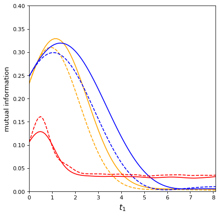
Figure 21: Comparison of the Gao-Jafferis teleportation protocol using either two copies of the $N$$=$$10$ SYK model, or two copies of the $N$$=$$10$ PG commuting model. Results are an ensemble average of 10 and 100 instantiations respectively, taking $\beta=1$, $\mu=\pm 0.139\pi$, and fixing the teleportation injection time as $t_{0}=-0.720$. Shown is the mutual information between the reference message qubit $R$ and the extracted final state message qubit $T$ as a function of the extraction time $t_{1}$. The PG commuting model results are shown for negative $\mu$ (solid red) and positive $\mu$ (dashed red). Results for the SYK model are shown for negative $\mu$ (solid orange) and positive $\mu$ (dashed orange). Also shown are results for the Learned17 SYK-based model introduced in Jafferis et al. (2022): for negative $\mu$ (solid blue) and positive $\mu$ (dashed blue).

B.3 Teleportation

We make a direct comparison of PG commuting and SYK-based models applying the teleportation protocol of Gao and Jafferis. Such a comparison did not appear in Gao (2023), where the analysis was limited to calculations that can be performed analytically in a certain approximation for the ensemble averaging. As for the OTOC comparisons of the previous section, we use the parameter choices from Gao (2023), which were tuned attempting to maximize the extent to which the non-holographic PG commuting models for a given $\beta$ can “mimic” behaviors of wormhole teleportation. Of course one does not expect to optimize the wormhole teleportation features of the SYK-based models for these same choices of parameters, so the comparison shown here essentially maximizes the potential to confuse holographic and non-holographic dynamics in the same teleportation protocol.

Figure 21 shows the comparison for $\beta=1$, with the mutual information plotted as a function of the extraction time $t_{1}$ for a fixed value of the injection time $t_{0}$. The $N$$=$$10$ SYK model shows the expected wormhole teleportation peak, with a larger peak for negative values of $\mu$, consistent with a negative energy pulse in the holographic dual description. The corresponding $N$$=$$10$ PG commuting model shows a much smaller peak, at a significantly earlier time, and with different late time behavior. Notably, the PG commuting model has a larger peak for positive values of $\mu$ rather than negative values, inconsistent with a holographic interpretation. In the same figure we also show results for the Learned17 model. As noted in the previous subsection, the Learned17 has a superficial similarity to the PG commuting models of Gao (2023). However, we see in Figure 21 that the teleportation behavior of the learned model tracks that of the SYK model, not that of the PG commuting model. We repeat that learned model was originally derived from the $N$$=$$10$ SYK model with $\beta=4$ and (in the conventions we use here) $\mu=\pm 0.095\pi$, with $t_{0}=-2.8$; nothing about the learning procedure, other than underlying holographic physics, would promote similarity to the SYK model for the parameter choices of Figure 21.

Figure 22: Comparison of PG commuting and SYK-based models. Results for the Gao-Jafferis protocol using a single instantiation of the SYK model with $N$$=$$20$, $q$$=$$4$, ${\cal J}$$=$$1$, $\beta$$=$$4$, and using $\mu$$=\pm 0.2$, compared with an ensemble average of 100 instantiations of the PG commuting model of Gao (2023) with the same parameter choices. Solid/dashed lines correspond to SYK/PG commuting models. Top: The mutual information $I(R$$:$$T)$ as a function of time $t_{0}$, for negative/positive values of $\mu$ (blue/orange lines). Second: The mean size of the thermal fermion operator. Third: $|Q|/P$ averaged over size. Bottom: The fitted linear slope of the phases of $Q^{\ell}(s)$.

Figure 23: Comparison of the distribution of the thermal fermion operator size. Left: The Gao-Jafferis protocol for a single instantiation of the SYK model with $N$$=$$20$, $q$$=$$4$, $\beta$$=$$4$, ${\cal J}$$=$$1$, and taking $t_{0}$$=$2.9. Shown are $|Q^{\ell}(s)|$ (blue) and $P^{\ell}(s)$ (orange) as a function of the operator size $s$; this is the same as Figure 8 but showing only the first fermion. Right: Ensemble average of 100 instantiations of the $N$$=$$20$ PG commuting model, also with $q$$=$$4$, $\beta$$=$$4$, ${\cal J}$$=$$1$, and taking $t_{0}$$=$1.4. The time chosen corresponds to the maximum slope of the phases from a weighted linear fit.

Figure 24: Size winding comparison for $N$$=$$20$ SYK-based and PG commuting models. Upper left: Size winding of the Gao-Jafferis protocol for a single instantiation of the SYK model with $N$$=$$20$, $q$$=$$4$, $\beta$$=$$4$, ${\cal J}$$=$$1$, $\mu$$=$$-0.2$, and taking $t_{0}$$=$2.9. This is the same example as in Figure 5 but showing only the size winding of the first fermion. Upper right: Ensemble average of 100 instantiations of the $N$$=$$20$ PG commuting model, also with $q$$=$$4$, $\beta$$=$$4$, ${\cal J}$$=$$1$, and taking $t_{0}$$=$1.4. The time chosen corresponds to the maximum slope of the phases from a weighted linear fit (upper black dashed line). The lower black dashed line is where the corresponding right size winding should lie, while the orange dashed line is a linear fit to the actual points after applying the Left-Right interaction. Lower: The same ensemble average of PG commuting models, looking now at time $t_{0}$$=$2.9, and averaged over the first 10 fermions. The black dashed line is a linear best fit with slope -0.002 $\pm 0.006$, i.e., consistent with an absence of size dependence in the phases of $Q^{\ell}(s)$.

B.4 Size winding

It is interesting to check if the PG commuting models can mimic the physics of size winding for parameter choices in the same range where the SYK-based models exhibit the size winding mechanism for quantum information transfer. In Figure 22 we show an average over 100 instantiations of the PG commuting model Gao (2023), using the same choice of parameters as for the Gao-Jafferis SYK-based example shown in Figure 5, i.e., $N$$=$$20$, $q$$=$$4$, $\beta$$=$$4$, ${\cal J}$$=$$1$, $\mu$$=\pm 0.2$. The top plot shows a comparison of the mutual information $I(R$$:$$T)$ for the two models. The Gao-Jafferis model shows the usual peaking behavior for negative $\mu$, while the PG commuting model shows no peaking and no asymmetry at all. Both models show the same nonzero $I(R$$:$$T)$ at $t_{0}$$=$$0$, corresponding to the direct transmission mechanism discussed in section III. For the PG commuting model the contributions to $I(R$$:$$T)$ appear to be a combination of the direct transmission and “peaked-size teleportation”. As is apparent in the second plot of Figure 22 and in Figure 23 (Right), the PG commuting model has an earlier scrambling time, $t_{0}$$\simeq$$2$, and already for $t_{0}$$=$$1.4$ the thermal fermion operator size is peaked around $N$$/$$2$. At this same early time the PG commuting model shows some linear size dependence of the phases of $Q^{\ell}(s)$, as seen in Figure 24 (Upper right); this possibility was already noted in Gao (2023). However the slope is much too small for the Left-Right interaction to convert Left size winding to Right size winding, so size winding is not a good description of the transfer of quantum information.

As already pointed out in section III, the direct transmission mechanism completely dies off by the scrambling time; thus for $t_{0}$$>$$2$ we expect the PG commuting model to display only “peaked-size teleportation”. The flat behavior of $I(R$$:$$T)$ of the PG commuting model for $t_{0}$$>$$2$ seen in Figure 5 (Top) is consistent with this. We furthermore see in Figure 5 (Bottom) that in the same regime there is no statistically significant dependence of the phases of $Q^{\ell}(s)$ on size. Thus for example with $t_{0}$$=$$2.9$, where the complete size winding mechanism works well for the SYK-based model - see Figure 24 (Upper left) - the phases in the PG commuting model shows no sign of size dependence - see Figure 24 (Lower).

None of the behaviors of the PG commuting model that we have displayed here resemble the SYK-based Learned17 model, which as shown in Jafferis et al. (2022) and Jafferis et al. (2023) exhibits excellent size winding.

B.5 Conclusions

In this appendix we have compared the interesting finite $N$ PG commuting models of Gao (2023) with the finite $N$ SYK and learned models of Jafferis et al. (2022), including for the choices of parameters determined in Gao (2023) as most likely to produce confusing similarities between the properties of these models, similarities that might confuse our ability to separate holographic from non-holographic behaviors when implementing the wormhole teleportation protocol.

Our results show no such confusion. This is a strong check that the results of Jafferis et al. (2022) for finite $N$, including the learned model used in the Google Sycamore experiment, are consistent with the expected properties of holographic wormhole dynamics.