A reference meteor magnitude for intercomparable fluxes
Abstract
The rate at which meteors pass through Earth’s atmosphere has been measured or estimated many times over; existing flux measurements span at least 12 astronomical magnitudes, or roughly five decades in mass. Unfortunately, the common practice of scaling flux to a universal reference magnitude of +6.5 tends to collapse the magnitude or mass dimension. Furthermore, results from different observation networks can appear discrepant due solely to the use of different assumed population indices, and readers cannot resolve this discrepancy without access to magnitude data. We present an alternate choice of reference magnitude that is representative of the observed meteors and minimizes the dependence of flux on population index. We apply this choice to measurements of recent Orionid meteor shower fluxes to illustrate its usefulness for synthesizing independent flux measurements.
1 Introduction
Historically, meteor shower activity has usually been measured in terms of zenithal hourly rate (ZHR), the number of meteors observed per hour by a visual observer under ideal conditions (Norton & Chitwood, 2008). The ZHR is related to but distinct from meteor flux (Rendtel, 2022). In recent decades, however, a number of research groups have begun to report meteor fluxes from camera networks or meteor radars (some examples include Campbell-Brown, 2004; Blaauw et al., 2016; Molau, 2022; Vida et al., 2022). These networks vary in sensitivity and coverage, and thus measure the meteor flux in different size regimes. For instance, the Southern Argentina Agile MEteor Radar (SAAMER) measures meteor fluxes down to a limiting equivalent optical magnitude of +9 (Bruzzone et al., 2021), while the NASA All-Sky Fireball Network has been used to measure the Perseid meteor shower flux to a limiting magnitude of approximately -3.5 (Ehlert & Erskine, 2020).
If the flux of a single meteor shower is measured simultaneously by several different networks with different limiting magnitudes, these fluxes can be combined to inspect the shower’s mass (or magnitude) distribution. For instance, Campbell-Brown et al. (2016) combined flux data from five different optical systems as well as the Canadian Meteor Orbit Radar (CMOR) in order to construct a mass distribution that spanned four decades in mass. Similarly, Blaauw (2017) combined radar, optical, and lunar impact data to construct a mass profile for the Geminids.
The determination of a network’s limiting magnitude, however, is not straightforward, as the detection limit usually varies over the detector’s field of view (FOV). For example, the distance from which meteors are viewed tends to vary within the FOV in a way that depends on FOV width and orientation; if the region surveyed by a portion of the FOV is more distant, the meteor must be brighter to be detected. One could address this by discarding all meteors that are too dim to be detected in any part of the field of view, but this typically results in a large reduction in the overall count.
The most common way to deal with a variable limiting magnitude is to divide the FOV into smaller pieces and scale the area of each piece to reflect its contribution to the overall flux, assuming that meteor magnitudes follow a power-law distribution (Kaiser, 1960; Koschack & Rendtel, 1990a; Bellot Rubio, 1994; Vida et al., 2022; Molau, 2022). This is known as the effective collection area method and is described in Section 2.1. Because the areas are scaled to correspond to a constant reference limiting magnitude, one can in theory choose any reference magnitude one likes, so long as the power-law assumption holds over the range of magnitudes considered. A common choice is to scale the flux to a constant limiting magnitude of +6.5 and/or convert to ZHR (e.g., Roggemans, 1989; Bruzzone et al., 2021; Molau, 2022; Vida et al., 2022) to facilitate comparisons with visual rates (Koschack & Rendtel, 1990b):
| (1) | ||||
| ZHR | (2) |
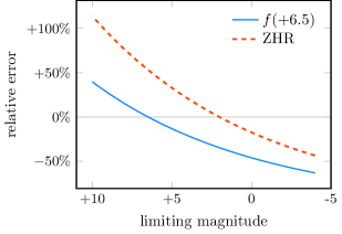
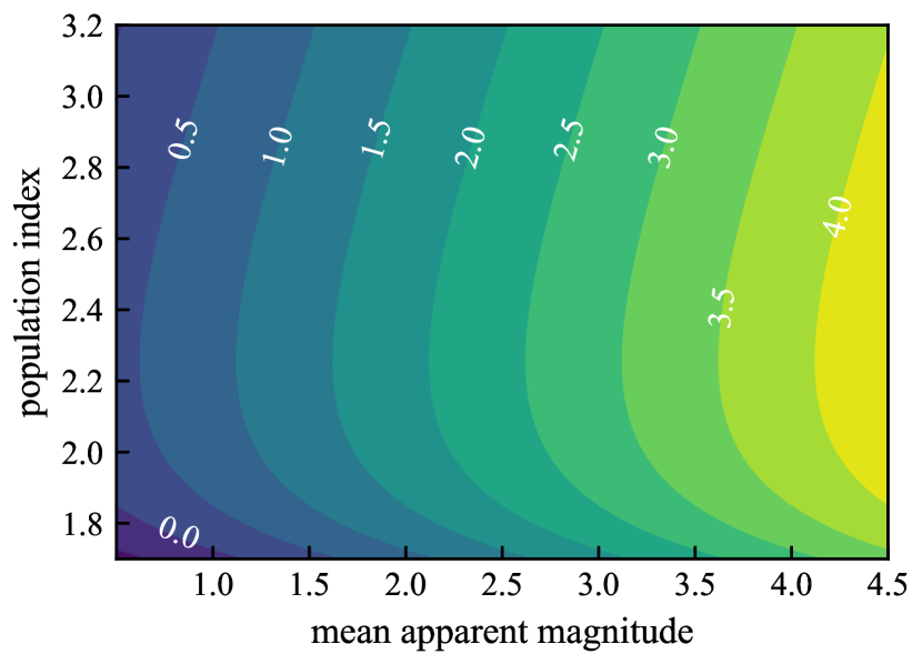
We use to denote the flux of meteors with absolute magnitudes brighter than , and we use to refer to the chosen reference magnitude. Notice that the above conversion depends on the assumed population index, ; if the flux is based on magnitudes that are very different from +6.5, the result can be quite sensitive to the choice of (see Figure 1). For example, if the meteor flux measured by CMOR is scaled from its limiting magnitude of +8 to an equivalent ZHR, but is used for a shower whose true value is , the ZHR will be inflated by 77%. Note that these fluxes include all meteors brighter than the given limiting magnitude. This is distinct from the dimmest apparent magnitude visible to a visual observer in the center of their visual field, which is also sometimes called the limiting magnitude (e.g., Koschack & Rendtel, 1990b), but which we call the visual limit.
Thus, while the use of a common limiting magnitude allows us to compare fluxes published by different groups using different data, it obscures the characteristic limiting magnitude of the system () and is sensitive to errors in the assumed magnitude distribution. If two independent flux measurements disagree, it can be unclear whether this is because the data are truly in conflict or because an incorrect choice of has been used. Even when it is clear that two sets of measurements use different values of , it is usually impossible for the reader to invert that choice unless magnitude information is also provided (or, in the case of the Video Meteor Network, a tool is provided that allows the reader to specify ; see Section 4.2). For this reason, the Campbell-Brown et al. (2016) and Blaauw (2017) studies exclusively used data from their own observation networks, which allowed them to enforce a consistent set of assumptions.
One possible solution to this problem of incompatible flux measurements is the choice of a reference magnitude that minimizes the dependence of the measured flux on population index. We derive an expression for such a reference magnitude in Section 2.2 that is compatible with the widely used “effective collection area” method of measuring fluxes. In Sections 2.3 and 2.4, we provide two alternative ways to estimate ; these estimates can be used by researchers to validate their flux calculations, and may in some cases enable readers to estimate for published fluxes. In Section 4, we apply these equations to several independent measurements of Orionid fluxes to demonstrate their value for synthesizing disparate measurements.
2 Reference limiting magnitude
The most common approach used to derive meteor flux from observed counts is the effective collection area (ECA) method. This method appears to have originated with Koschack & Rendtel (1990a) and Koschack & Rendtel (1990b), who used a similar approach to estimate the number of meteors that can be detected by a visual observer. Bellot Rubio (1994) adapted the approach to compute fluxes from camera data. These efforts were predated by Kaiser (1960), who developed an equivalent approach for radar data.
Today, it is widely used within the meteor astronomy community (recent examples include Blaauw, 2017; Margonis et al., 2019; Molau, 2022; Vida et al., 2022). We review this method in Section 2.1. We then derive a reference magnitude in Section 2.2 that minimizes the dependence of flux on population index.
We do not specify a method for determining the limiting magnitudes of a meteor observation network; this will depend on the properties of the network and the meteor detection algorithm. Our assumptions are that the limiting magnitude of the network has been characterized and that the ECA method is being used to measure fluxes. We refer readers to Molau et al. (2016) and Vida et al. (2022) for more information about the calculation of optical limiting magnitudes, and to Kaiser (1960) for an analogous discussion of radar fluxes. We do, however, offer an alternate method for estimating the reference magnitude that can be used to test whether the limiting magnitudes have been correctly calculated (see Section 2.4).
2.1 The effective collection area (ECA) method
Let denote the flux of meteors brighter than reference magnitude . The observed number of meteors follows a Poisson distribution with an expected value of
| (3) |
where is the number of meteors brighter than magnitude passing through area within time interval . If the meteors belong to a shower, they share a common velocity vector ; the unit vector is aligned with the meteors’ velocity vector. Note that is the meteor’s motion through space, and not its apparent angular motion; the latter plays a role in determining the limiting magnitude (Kingery & Blaauw, 2017; Molau et al., 2016).
If the collection area is flat and its normal vector points toward zenith, then the area presented to the shower is
| (4) |
where is the angle between the local zenith and the shower radiant (also known as the zenith angle). However, meteors entering the atmosphere at a high angle of incidence encounter a gentler atmospheric density gradient along their path, which is thought to decrease their peak brightness (Zvolánková, 1983). Both Zvolánková (1983) and Molau & Barentsen (2013) suggest that this can be handled by applying an exponent to the zenith angle term:
| (5) |
where the constant varies between showers but is approximately 1.5-2.
As discussed in Section 1, the limiting meteor magnitude typically varies within the field of observation. The ECA method handles this by dividing the field of view into a grid and assuming that the limiting magnitude does not vary appreciably within a grid cell. If cell covers area and has limiting meteor magnitude , then the expected number of meteors in that cell is
| (6) |
Recall from equation 1 that the relationship between limiting magnitude and flux is a power law; that is,
| (7) |
where is the population index. Therefore,
| (8) |
The sum of a set of independent Poisson random variables is itself a Poisson random variable, and its expected value is the sum of the expected values of its components. Thus, the expected total number of observed meteors across all cells is
| (9) |
where the quantity in parentheses is called the effective collection area:
| (10) |
Equation 9 can then be rewritten as
| (11) |
The observed number of events, , is an unbiased estimate for the rate of the Poisson process. Therefore, we estimate the flux as
| (12) |
and recover (for example) Equation 1 of Molau (2022).
Note that if varies smoothly across the FOV, one could replace the sum in Equation 10 with an integral. For instance, Kaiser (1960) integrates the equivalent of along the radar echo line; see Equation 18 of that paper. However, most optical applications of the ECA methods use the discrete form presented here.
2.2 Derivation of reference magnitude
We seek a reference limiting magnitude that minimizes the dependence of flux on population index. To obtain this, we set
| (13) |
It can be shown that is zero when:
| (14) |
We see from this equation that the optimal reference magnitude is a weighted average of the limiting magnitudes of each cell, and therefore lies within the network’s limiting magnitude range.
If we multiply both the numerator and denominator of equation 14 by , , , and , we find that can re-write equation 14 as follows:
| (15) |
We see that the weights are proportional to the expected number of meteors in each cell. Thus, is a weighted average of the limiting magnitude (which is used by Vida et al., 2022), where the weights are the expected rates for each cell.
2.3 Average limiting magnitude per meteor
The form of equation 15 hints that we can estimate the reference magnitude using the observed meteor counts:
| (16) |
Notice that we have replaced the expected counts, , with the observed counts, . This approximation makes it clear that our proposed reference magnitude not only lies within the network’s range of limiting magnitudes, but is in fact the per-meteor mean limiting magnitude. This makes a doubly appealing choice in that it is representative of the limiting magnitude distribution in addition to minimizing the dependence on .
We suggest that researchers publishing fluxes verify that the approximation given in equation 16 is similar to the true value given by equation 14. A large discrepancy could indicate that either the cell areas or population index are incorrect. We will also show in an upcoming paper that equation 16 provides a reference magnitude that minimizes the covariance between flux and population index when fitting for both quantities simultaneously.
If we use the sample mean of the limiting magnitude (Eq. 16) as a reference magnitude, then a sensible extension is to use the sample standard deviation of the limiting magnitude to describe the range of limiting magnitudes within a meteor detection network:
| (17) |
If the distribution of limiting magnitudes is strongly skewed or multi-model, researchers could consider quoting another measure of variation, such as the interquartile range.
2.4 Average absolute magnitude
If we assume that places a strict upper limit on the absolute meteor magnitude that can be observed in cell , then the probability of observing a meteor with absolute magnitude in that cell is:
| (18) |
Using this probability distribution, we can calculate the average absolute magnitude we expect for meteors in that cell:
| (19) |
We see that the average observed magnitude in any given cell should be systematically offset from the limiting magnitude in that cell by a constant value of . Furthermore, the probability that a meteor is detected in a cell with limiting magnitude is:
| (20) |
We can now combine equations 19 and 20 to obtain the expected absolute magnitude of a meteor detected by the system:
| (21) |
If we substitute the mean absolute meteor magnitude for the expected absolute meteor magnitude, equation 21 provides yet another estimate of :
| (22) |
Here we use the index to emphasize that this sum is performed over all meteors rather than all cells. This estimate depends only on the observed absolute magnitudes and the population index; it does not depend at all on the cell-specific limiting magnitudes.
Equation 21 has two important uses. First, it can be compared with equation 16 to determine whether the limiting magnitudes have been computed correctly. Second, it may be useful for estimating the reference limiting magnitude associated with a published flux value when only meteor counts and magnitudes are provided.
3 Inapplicability to visual rates
The ECA method as presented in Section 2.1 assumes that every meteor that is bright enough to be detected in a given cell will be detected. However, Koschack & Rendtel (1990a) found that there is no hard upper limit on meteor magnitude when it comes to human observers; instead, the probability of detection varies with the brightness of the meteor and its angular offset from the observer’s line of sight. As a result, Equations 14, 16, and 22 cannot be applied to visual observations; we derive an alternative in this section.
Equations 1 and 2 can be combined:
| (23) |
If we then set the derivative of this equation with respect to to zero, we obtain:
| (24) |
However, equation 23 does not account for observing conditions. If a visual observer is viewing a hazy or light-polluted sky, they may not be able to detect meteors down to magnitude +6.5. We seek a reference magnitude that takes this into account.
We have been unable to reproduce the derivation of equation 2 from the information provided in Koschack & Rendtel (1990a) and Koschack & Rendtel (1990b). We nevertheless have attempted to simulate a reasonable range of magnitudes that is consistent with their general approach. First, we constructed an empirical profile for airmass vs. elevation angle () by repeatedly evaluating the following integral for different choices of :
| (25) | ||||
| (26) |
where is the Earth’s radius, is the air density, and the integration variable is distance from the observer. We performed this task using the “StandardAtmosphereData” function in Mathematica (Wolfram Research, Inc., 2023), which defaults to the 1976 United States Standard Atmosphere model (United States Committee on Extension to the Standard Atmosphere (1976), COESA).
Next, we divided the visible sky into bins and calculated the elevation angle and distance corresponding to each bin, assuming that meteors ablate at a height of 100 km. The limiting magnitude of each bin is then:
| (27) |
where is the visual limit, the dimmest magnitude of an object visible to the observer.
Although Koschack & Rendtel (1990a) did not settle on a satisfactory functional form for the probability of perception, we were able to approximate Table 4 of Koschack & Rendtel using the following formula:
| (28) | ||||
| (29) |
Here “expit” is the standard logistic function, is apparent meteor magnitude, is the angular separation between the observer’s line of sight (LOS) and the meteor, and the constants are , , and . This approximation gives us values that are typically within 0.05 of the correct fractional value.
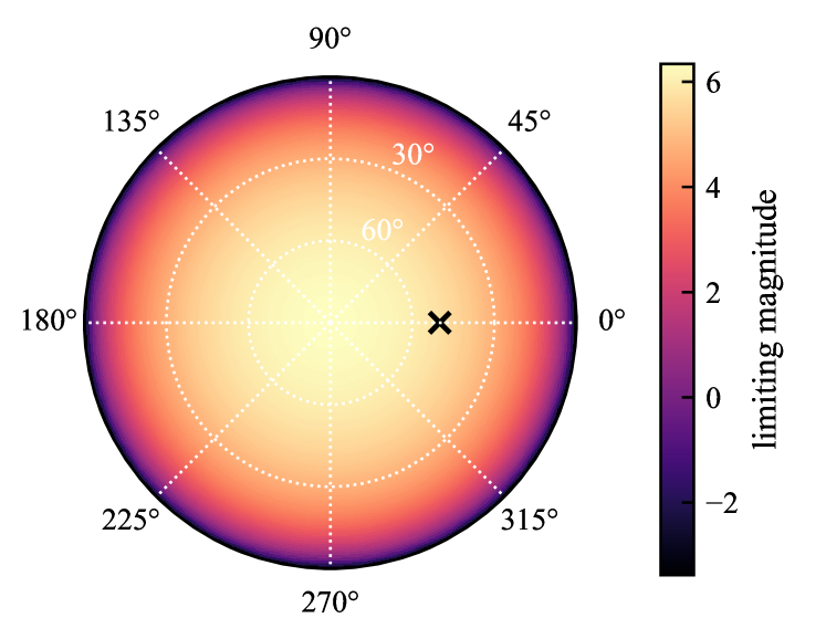
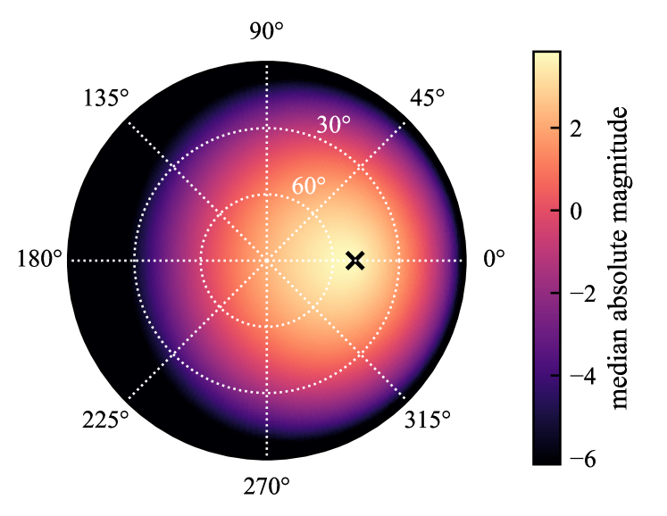
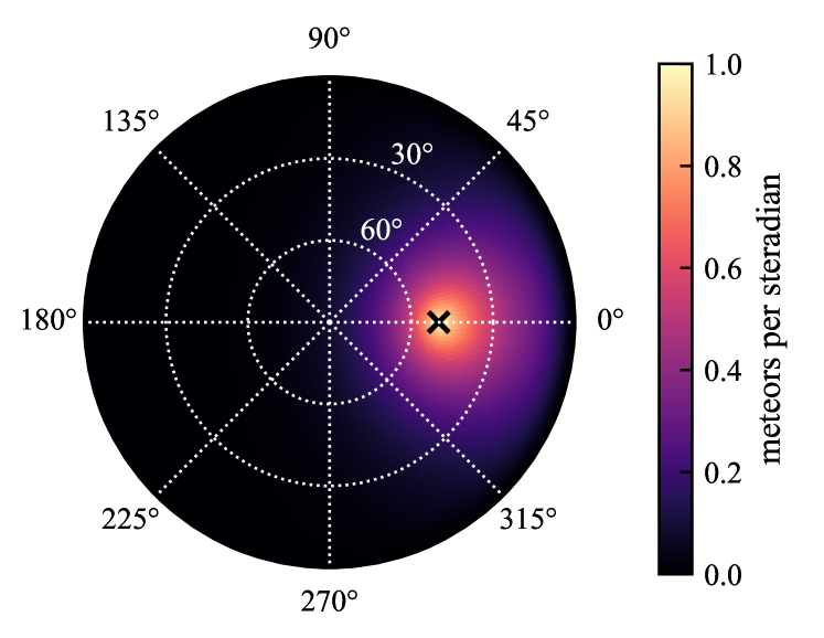
We can see from Equation 28 that the probability of observing a meteor right at the limit of detectability () is quite low, even in the center of the observer’s field of view (, ). The observer has a much better chance of observing meteors that are several magnitudes brighter than the detectability limit and that pass near the direction of their gaze. As a result, the typical magnitude observed will be quite a bit brighter than the limiting magnitude, especially in the peripheral visual field. This effect is illustrated in Figure 2.
The probability of perception complicates the determination of the reference magnitude. The number of meteors we expect to see in a given area is now:
| (30) |
where is the fraction of all meteors we expect to see in that area:
| (31) |
Because is a function of , it must be included in our calculation of . Equation 14 is replaced with:
| (32) |
This equation must be evaluated numerically. We have done so, using a range of plausible values, and found that
| (33) |
The two expressions agree to within 0.2 magnitudes between and . Furthermore, we find that the average apparent magnitude can be approximated as follows:
| (34) |
This expression allows us to estimate the visual limit from the mean apparent magnitude. Assuming the classical +6.5 limit, the mean apparent magnitude will be approximately +2.9 for .
If we combine equations 24, 33, and 34, we can estimate the reference magnitude directly from the mean apparent magnitude:
| (35) |
This approximate reference magnitude has both of our desired qualities: it minimizes the dependence of flux on and it is representative of the range of magnitudes observed. It does, however, require observers to record the apparent magnitudes of individual meteors; fortunately, the International Meteor Organization (IMO) Visual Meteor Database (VMDB) includes apparent magnitudes for a subset of all observations.
We would like to point out that our treatment of ZHR and reference magnitude neglects the difference between visual and camera or photometric magnitude. For instance, Jacchia (1957) found that visual magnitude estimates were 1-2 magnitudes brighter than photographic magnitude measurements for the same meteors. This difference, which they call the “color index,” is a function of photographic magnitude (see Figure 12b of that paper) and is attributed to the Purkinje effect (see also Protte & Hoffmann, 2020). If we assume that the perception probability applies to visual magnitude and use another sigmoid function to describe the color index, we predict an average apparent visual magnitude that is about half a magnitude dimmer than Equation 34. Unfortunately, Equation 31 becomes quite complicated in this case. A full treatment of this effect is beyond the scope of this paper; for now, we will simply consider the uncertainty associated with Equation 35 to be at least 0.5 magnitudes.
We began this section by drawing a distinction between the hard detection threshold assumed for instrumental detection and the lack of such a threshold for visual observations. However, instrumental detection thresholds will also be “softened” to some extent by noise. If the magnitude range of this softening effect is non-negligible compared to the range of detected magnitudes in the cell or the range of limiting magnitudes represented in the network, then the use of the ECA method – and Equations 14, 16, and 22 – may not be appropriate.
4 Application to the Orionids
In this Section, we compare fluxes from four independent meteor observation networks and demonstrate the benefit of using our proposed reference magnitude. These networks are the Global Meteor Network (GMN; Vida et al., 2021), the IMO Video Meteor Network (VMN; Molau & Barentsen, 2014), the IMO Visual Meteor Database (VMDB; Roggemans, 1988), and the Canadian Meteor Orbit Radar (CMOR; Jones et al., 2005).
We selected the Orionids for this demonstration because all four networks assume quite different values of for this shower (see Table 1). Normally, this would prohibit a useful synthesis of the data. However, we will attempt to estimate the reference magnitude of each network and show that this removes some of the discrepancy in activity. We include the past four years of Orionid activity; this choice is determined by GMN, whose fluxes date back to 2020.
All three flux networks (GMN, VMN, and CMOR) use the same flux-to-ZHR conversion (eqs. 1 and 2). Thus, once we determine for each network, we can convert the published ZHR values for that network to by inverting these equations, using each source’s assumed .
| network | |||
|---|---|---|---|
| CMOR | 3.0 | +8.0 | |
| GMN | 2.2 | +3.9 | |
| VMN | 2.5 | +2.0 | |
| VMDB | 2.4 | +2.6 |
Note – The population index () listed is the value used to calculate meteor flux or ZHR by each network. We also include our estimated reference magnitude ( or ) for each network where applicable.
4.1 Global Meteor Network (GMN)
GMN meteor fluxes are already reported to the appropriate reference magnitude (Equation 14; these are called time-area-product or TAP-weighted magnitudes in Vida et al., 2022). In fact, the GMN flux data files report the reference magnitude for each observation interval as well as the overall average; the reference magnitude may vary over time due to changes in observing conditions (Vida et al., 2022). In Table 1, we report the reference magnitude averaged over all years.
4.2 Video Meteor Network (VMN)
VMN fluxes can be obtained from a web portal111https://meteorflux.org/; these fluxes are quoted to magnitude +6.5 and are also converted to ZHR. We used the default options for the Orionids, with one exception: we opted to turn on the perception coefficient (PC) correction.
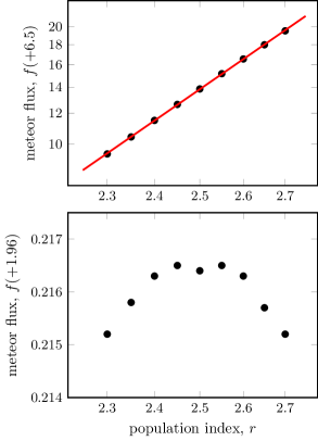
The website does not report meteor magnitudes, but it does allow the user to vary the assumed population index (Molau et al., 2014). This gives us an opportunity to extract using yet another approach. Using equation 1, we calculate:
| (36) |
Because , we can therefore obtain by repeatedly changing the assumed value of and regressing the reported against . The results of this process are shown in the top panel of Figure 4. We obtain in this manner. The bottom panel of Figure 4 demonstrates that this value does in fact minimize the variation in flux; when we use , the variation in flux over to is less than 1%, which is much less than the factor-of-two range we see in . Figure 4 also indicates that there is some noise in the data, which is probably due to rounding error; we therefore round our reference magnitude to +2.
4.3 Visual Meteor Database (VMDB)
Zenithal hourly rates (ZHR) for major showers are published by the International Meteor Organization (IMO) on their website.222https://www.imo.net/members/imo_live_shower These ZHRs are automatically computed from user-supplied data and the IMO does not recommend their use for scientific applications. We ignored this warning for the purposes of this demonstration and downloaded Orionid ZHR values for the years 2020 through 2023. The IMO uses for the “whole campaign.”
Magnitude counts are available to IMO members via the Video Meteor Database (VMDB).333https://www.imo.net/members/imo_vmdb We downloaded these data for Orionids between 2020 and 2023 (inclusive). Because visual observations do not contain distance information, these are apparent magnitudes; we found that the mean apparent magnitude was +2.75. When we input this value, along with into equation 35, we obtain a reference magnitude of .
4.4 Canadian Meteor Orbit Radar (CMOR)
CMOR is a patrol radar; it detects the reflection of an emitted radar pulse off of the surface of the cylinder of plasma produced by an ablating meteor. The ability to detect a meteor is therefore not determined by its brightness, but rather by the electron line density of the trail (usually denoted ). Furthermore, CMOR does not necessarily detect the meteor when its trail is at its peak electron line density. Instead, it detects a meteor when its velocity has no radial component relative to the radar station and its trail is therefore perpendicular to the radar beam.
Electron line density can be converted to an equivalent radar magnitude, but individual radar magnitudes are not readily available for those meteors contributing to the Orionid fluxes measured by CMOR. However, the CMOR flux pipeline accepts population index (in the form of a mass index) as an input parameter. We therefore varied in order to extract using the approach outlined in 4.2. We found that , which is fairly close to the limiting magnitude of +8.4 quoted in Campbell-Brown (2004).
4.5 Synthesis
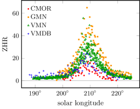
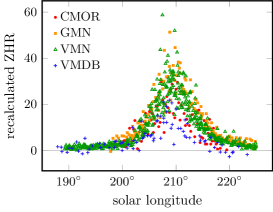
The raw ZHR values reported for each network are shown in Figure 5. The peak values are quite discrepant; the CMOR and VMDB data have a peak ZHR of approximately 15, the VMN data have a peak ZHR of about 30, and the GMN data have a peak ZHR of about 50.
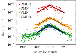
We convert ZHR to flux using equation 23 and each network’s chosen value of . We also fit a double-exponential function (Jenniskens, 1994) to the data in order to extract the peak value. Some of the data in Figure 5 show signs of sporadic contamination; for instance, both video networks appear to asymptote around . We therefore simultaneously fit for a constant background level and subtract it from the flux. The results are shown in Figure 6.
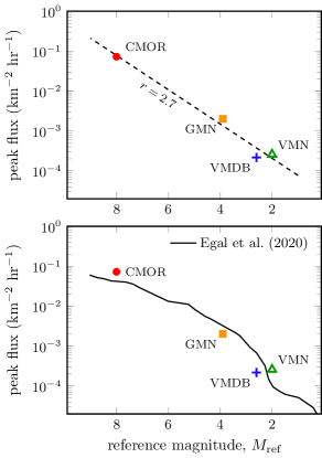
Our profile fits allow us to extract the peak ZHR or flux from each data set. These peak fluxes are then plotted against the reference magnitudes in Figure 7. If the mass distribution does indeed take the shape of a power law, then this plot should resemble a line. If we fit for using these four points, we obtain an overall population index of (corresponding to a peak ZHR of 28). On the other hand, the Orionid mass distribution may not resemble a power law over large ranges in mass. The dynamical simulations of Egal et al. (2020) predict a relative lack of Orionid particles at sizes that are roughly comparable with CMOR’s limiting magnitude. In the bottom panel of Figure 7, we compare our peak fluxes with the relative particle counts shown in Figure 13 of Egal et al. (2020), extracted using WebPlotDigitizer (Rohatgi, 2022). Masses have been converted into magnitudes using the mass-magnitude relation of Verniani (1973), and an arbitrary scaling has been applied to the particle counts to bring them into rough agreement with the data. Both distributions appear to be plausible matches to the data.
Although we have obtained using the measurements discussed in this paper, we do not suggest that the meteor astronomy community should necessarily adopt this value for the Orionid meteor shower. Our intent is instead to demonstrate how our proposed reference magnitude can be used to better compare disparate results. When fluxes are quoted to a network-specific reference magnitude, we can combine independent measurements to probe the magnitude distribution and reveal any remaining discrepancies. For instance, if we convert flux back to ZHR using for all networks, we find that the discrepancy between networks has been reduced (see Figure 8), but not eliminated. The spread in peak ZHR values has been reduced by approximately one-third (see Table 2). The visual rates are still lower than the instrumentally measured rates but, because we have accounted for differences in the assumed value of , we now know that this discrepancy must be due to some other factor.
| network | ZHR | ZHR |
|---|---|---|
| CMOR | 15.3 | 25.7 |
| GMN | 51.3 | 41.1 |
| VMN | 31.8 | 34.3 |
| VMDB | 15.3 | 16.0 |
5 Conclusion
Currently, meteor fluxes are typically scaled to ZHR or a standard limiting magnitude of +6.5 prior to publication. We argue that fluxes should be reported to a network-specific reference magnitude that is equal to a weighted average of the limiting magnitude of the observing station(s). This choice of reference magnitude minimizes the dependence of the reported flux on the assumed population index and therefore enables the synthesis of independent meteor shower flux measurements. This is particularly useful when the population index varies with magnitude, as the index that is most appropriate for computing flux from a particular set of observations may differ from the average index over a large range of magnitudes.
If researchers choose to publish fluxes using our suggested reference magnitude, we suggest that they also include some measure of the degree of variation within their network’s limiting magnitude. We have suggested the sample standard deviation of the limiting magnitude. If the variation in limiting magnitude is very large and if there are a sufficient number of meteor detections, the researcher could also consider subdividing the data into magnitude ranges (e.g., Molau et al., 2014).
In many cases, fluxes are quoted to a minimum mass rather than limiting magnitude. We favor the use of a reference magnitude rather than a reference mass for two reasons. First, magnitude is more closely related to the observed quantity: the apparent brightness seen by the observer or observing station. This is reflected in the effective collection area method for measuring fluxes, which depends only on limiting magnitude. The second reason is that there are multiple competing formulae for converting magnitude to mass (Jacchia et al., 1967; Verniani, 1973; Campbell-Brown et al., 2016), and therefore the conversion of magnitude to mass creates another opportunity to introduce discrepancies that arise from different assumptions rather than real differences in the data.
To demonstrate the utility of our reference magnitude, we estimated its value for several independent measurements of Orionid fluxes between 2020 and 2024. We included data from four networks, each of which used a different assumed population index to compute meteor flux or ZHR. We found that the data could be brought into closer agreement if we assume that the Orionid mass index is approximately 2.7. This synthesis could potentially be improved if exact, rather than estimated, reference magnitudes for CMOR and VMN were to be published. The data also suggest that a meteor observation network of extremely sensitive cameras with a reference magnitude of approximately +6 (similar to electron-multiplied charge-coupled device, or EMCCD, cameras; Brown & Weryk, 2020; Mills et al., 2021; Gural et al., 2022) would be a valuable addition.
This work was supported in part by NASA Cooperative Agreement 80NSSC21M0073 and by the Natural Sciences and Engineering Research Council of Canada.
References
- Bellot Rubio (1994) Bellot Rubio, L. R. 1994, WGN, Journal of the IMO, 22, 118
- Blaauw (2017) Blaauw, R. C. 2017, Planetary and Space Science, 143, 83, doi: 10.1016/j.pss.2017.04.007
- Blaauw et al. (2016) Blaauw, R. C., Campbell-Brown, M., & Kingery, A. 2016, MNRAS, 463, 441, doi: 10.1093/mnras/stw1979
- Brown & Weryk (2020) Brown, P., & Weryk, R. J. 2020, Icarus, 352, 113975
- Bruzzone et al. (2021) Bruzzone, J. S., Weryk, R. J., Janches, D., et al. 2021, The Planetary Science Journal, 2, 56, doi: 10.3847/PSJ/abe9af
- Campbell-Brown (2004) Campbell-Brown, M. D. 2004, MNRAS, 352, 1421, doi: 10.1111/j.1365-2966.2004.08039.x
- Campbell-Brown et al. (2016) Campbell-Brown, M. D., Blaauw, R., & Kingery, A. 2016, Icarus, 277, 141, doi: 10.1016/j.icarus.2016.05.001
- Egal et al. (2020) Egal, A., Wiegert, P., Brown, P. G., Campbell-Brown, M., & Vida, D. 2020, Astronomy and Astrophysics, 642, A120, doi: 10.1051/0004-6361/202038953
- Ehlert & Erskine (2020) Ehlert, S., & Erskine, R. B. 2020, Planetary & Space Science, 188, 104938, doi: 10.1016/j.pss.2020.104938
- Gural et al. (2022) Gural, P., Mills, T., Mazur, M., & Brown, P. 2022, Experimental Astronomy, 53, 1085, doi: 10.1007/s10686-021-09828-3
- Jacchia et al. (1967) Jacchia, L., Verniani, F., & Briggs, R. E. 1967, Smithsonian Contributions to Astrophysics, 10, 1
- Jacchia (1957) Jacchia, L. G. 1957, Astronomical Journal, 62, 358, doi: 10.1086/107551
- Jenniskens (1994) Jenniskens, P. 1994, Astronomy and Astrophysics, 287, 990
- Jones et al. (2005) Jones, J., Brown, P., Ellis, K. J., et al. 2005, Planetary and Space Science, 53, 413, doi: 10.1016/j.pss.2004.11.002
- Kaiser (1960) Kaiser, T. 1960, MNRAS, 121, 284, doi: 10.1093/mnras/121.3.284
- Kingery & Blaauw (2017) Kingery, A., & Blaauw, R. C. 2017, Planetary and Space Science, 143, 67, doi: 10.1016/j.pss.2017.03.006
- Koschack & Rendtel (1990a) Koschack, R., & Rendtel, J. 1990a, WGN, Journal of the IMO, 18, 44
- Koschack & Rendtel (1990b) —. 1990b, WGN, Journal of the IMO, 18, 119
- Margonis et al. (2019) Margonis, A., Christou, A., & Oberst, J. 2019, Astronomy & Astrophysics, 626, A25, doi: 10.1051/0004-6361/201834867
- Mills et al. (2021) Mills, T., Brown, P. G., Mazur, M. J., et al. 2021, MNRAS, 508, 3684
- Molau (2022) Molau, S. 2022, WGN, Journal of the IMO, 50, 126
- Molau & Barentsen (2013) Molau, S., & Barentsen, G. 2013, in Proceedings of the International Meteor Conference, 31st IMC, La Palma, Canary Islands, Spain, 2012, ed. M. Gyssens & P. Roggemans, 11–17
- Molau & Barentsen (2014) Molau, S., & Barentsen, G. 2014, in Meteoroids 2013, ed. T. J. Jopek, F. J. M. Rietmeijer, J. Watanabe, & I. P. Williams, 297–305
- Molau et al. (2014) Molau, S., Barentsen, G., & Crivello, S. 2014, in Proceedings of the International Meteor Conference, Giron, France, 18-21 September 2014, ed. J. L. Rault & P. Roggemans, 74–80
- Molau et al. (2016) Molau, S., Crivello, S., Goncalves, R., et al. 2016, WGN, Journal of the IMO, 44, 120
- Norton & Chitwood (2008) Norton, O. R., & Chitwood, L. A. 2008, Field Guide to Meteors and Meteorites (London: Springer-Verlag), doi: 10.1007/978-1-84800-157-2
- Protte & Hoffmann (2020) Protte, P., & Hoffmann, S. M. 2020, Astronomische Nachrichten, 341, 827, doi: 10.1002/asna.202013803
- Rendtel (2022) Rendtel, J. 2022, Handbook for Meteor Observers, 3rd edn. (International Meteor Organization)
- Roggemans (1988) Roggemans, P. 1988, WGN, Journal of the IMO, 16, 179
- Roggemans (1989) —. 1989, Handbook for Visual Meteor Observations (Cambridge, Mass.: Sky Publishing Corp.)
- Rohatgi (2022) Rohatgi, A. 2022, Webplotdigitizer: Version 4.6. https://automeris.io/WebPlotDigitizer
- United States Committee on Extension to the Standard Atmosphere (1976) (COESA) United States Committee on Extension to the Standard Atmosphere (COESA). 1976, U.S. Standard Atmosphere, 1976, NOAA-S/T-76-1562 (National Oceanic and Atmospheric Administration). https://ntrs.nasa.gov/citations/19770009539
- Verniani (1973) Verniani, F. 1973, Journal of Geophysical Research, 78, 8429, doi: 10.1029/JB078i035p08429
- Vida et al. (2022) Vida, D., Blaauw Erskine, R. C., Brown, P. G., et al. 2022, MNRAS, 515, 2322, doi: 10.1093/mnras/stac1766
- Vida et al. (2021) Vida, D., Šegon, D., Gural, P. S., et al. 2021, MNRAS, 506, 5046, doi: 10.1093/mnras/stab2008
- Wolfram Research, Inc. (2023) Wolfram Research, Inc. 2023, Mathematica, 13.3.0.0, Wolfram Research, Inc. https://www.wolfram.com/mathematica
- Zvolánková (1983) Zvolánková, J. 1983, Bulletin of the Astronomical Institutes of Czechoslovakia, 34, 122