We propose a method for constructing a confidence region for the solution to a conditional moment equation. The method is built around a class of algorithms for nonparametric regression based on subsampled kernels. This class includes random forest regression. We bound the error in the confidence region’s nominal coverage probability, under the restriction that the conditional moment equation of interest satisfies a local orthogonality condition. The method is applicable to the construction of confidence regions for conditional average treatment effects in randomized experiments, among many other similar problems encountered in applied economics and causal inference. As a by-product, we obtain several new order-explicit results on the concentration and normal approximation of high-dimensional -statistics.
Keywords: Random Forest Regression, Half-Sample Bootstrap, -statistics
JEL: C01, C14, C12
1. Introduction
Consider an independent and identically distributed sample , where each observation can be partitioned . We study a method for constructing a uniform confidence region for the parameter vector , where each is the unique scalar solution to the conditional moment equation
| (1.1) |
in and is a specified -vector in the domain of . Here, is an unknown nuisance parameter, identified via an auxiliary statistical problem, and is a known moment function. Many problems in applied economics and causal inference can be formulated as instances of (1.1), including nonparametric regression, quantile regression, and estimation of conditional average treatment effects.
To fix ideas, consider Banerjee et al., (2015), who study the effects of a poverty alleviation program implemented in Ghana.111Banerjee et al., (2015) study data collected from several similar graduation programs. We focus on the data from their evaluation of the program implemented in Ghana. Appendix E gives further details on our treatment of the Banerjee et al., (2015) data. For each individual in their sample, they observe the data , where is a measurement of total assets taken two years after the implementation of the program, is an indicator denoting assignment to the program, and is a vector of covariates. A broad aim of the study is to determine the conditions under which recipients of aid experience lasting improvements in welfare. One quantity that can inform this determination is the conditional average treatment effect (CATE)
| (1.2) |
where and are the potential outcomes generated by the intervention and is some chosen subvector of . A canonical approach to estimating (1.2) is premised on the observation that is the solution to the moment equation
| (1.3) |
of Robins et al., (1994) and Hahn, (1998), where the nuisance parameter collects the conditional outcome regression and Horvitz-Thompson weight
| (1.4) |
for the propensity score . See e.g., Nie and Wager, (2021), Foster and Syrgkanis, (2023), and references therein for further discussion.
Often, estimates of solutions to conditional moment equations of the form (1.1) or (1.3) are obtained by solving the empirical conditional moment equation
| (1.5) |
in , where is some first-stage estimator of the nuisance parameter and is some, potentially random and data-dependent, kernel function measuring the distance between and . Subsampled or bagged kernels, introduced by Breiman, (1996), and popularized by Wager and Athey, (2018) and Athey et al., (2019), are particularly convenient, due in part to their computational efficiency and robustness to tuning parameter choice. Popular examples of subsampled kernel estimators include -NN regression (Fix and Hodges,, 1989) and random forest regression (Breiman,, 2001). Solutions to conditional moment equations (1.5) constructed with random forest regression are referred to as Generalized Random Forests (GRF) (Athey et al.,, 2019).
Figure 1 displays GRF estimates of the CATE (1.2) for the experiment studied in Banerjee et al., (2015), where the chosen conditioning covariates are pretreatment measurements of monthly consumption and total assets.222These estimates are constructed by approximating the solution to the conditional moment (1.3) with a subsampled kernel estimator of the form (1.5) at each point on a grid. Both the nuisance parameter estimator and the kernel are constructed with the implementation of random forest regression made available through the “GRF” R package (Athey et al.,, 2019). The graduation program appears to be most effective for individuals with high level of baseline consumption and a low level of baseline assets.333The quartiles of baseline log consumption are 3.33, 3.76, and 4.20. The quartiles of baseline assets are -0.45, -0.71, and 0.03. Panel A of Figure E.4 displays of scatter plot of the joint distribution of baseline log consumption and assets. That is, individuals with an opportunity to increase their assets are able to do so only if they have a high level of baseline consumption. The effect of the program for individuals with low baseline consumption or high baseline assets appears more muted. These results are suggestive of a poverty trap: individuals without a stable source of consumption may be incentivized to sell productive assets (Kraay and McKenzie,, 2014; Balboni et al.,, 2022).
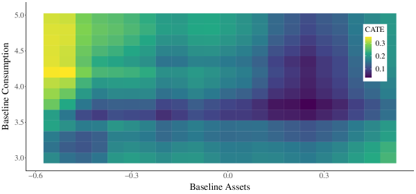 |
Notes: Figure 1 displays a heat map giving CATE estimates for the intervention studied in Banerjee et al., (2015) on post-treatment assets. The color of each rectangle indicates the estimate of the CATE queried at the rectangle’s central point. The horizontal and vertical axes display the baseline monthly consumption, normalized to dollars and measured in logs base 10, and the baseline value of an index for total assets. CATE estimates are obtained by solving the empirical moment equation (1.5) for each value on an evenly spaced grid on both axes. The nuisance parameter estimate and the kernel are constructed with the implementation of random forest regression made available through the “GRF” R package (Athey et al.,, 2019). See Appendix E for further details.
The information communicated by Figure 1 is rich and granular. This contrasts with the more widely encountered practice of reporting regression coefficients on linear interactions of pretreatment covariates with treatment indicators. In fact, as we will see, the latter approach gives a substantively different picture of the heterogeneity in the effect of the Banerjee et al., (2015) graduation program.
We contribute a method for assessing the statistical significance of estimates typified by Figure 1. In particular, we propose a computationally simple procedure for constructing uniform upper and lower confidence bounds for solutions to conditional moment equations (1.1) centered around subsampled kernel estimators of the form (1.5). Formally, we construct a family of random intervals
| (1.6) |
on the basis of the observed data, such that
| (1.7) |
for some sequence , where is some statistical family that contains the distribution of the data . We say that a region (1.6) satisfying (1.7) is uniformly asymptotically valid at the rate . Here, uniformity operates over both the -dimensional query-vector and the statistical family .444Following Li, (1989), uniform validity of a confidence region for nonparametric regression is often referred to as “Honesty” (see., e.g., Chernozhukov et al., (2014); Armstrong and Kolesár, (2020); Kuchibhotla et al., (2023)). We use the label “uniform validity,” following e.g., Romano and Shaikh, (2012), to distinguish this property from “Honest” construction of subsampled kernels (Athey and Imbens,, 2016; Wager and Athey,, 2018), which will be studied in detail in Section 3. The main theoretical contribution of this paper is the construction of uniform asymptotically valid confidence regions whose error rate converges to zero in asymptotic regimes where the number of points in the query-vector may increase much more quickly than the sample size .555The leading examples for choices of the query-vector are cases where is taken to be the observed values of the covariates or where gives a fine grid over the domain of . In both cases the dimension of the query-vector is either equal to or potentially large relative to the sample size .
We begin, in Section 2, by defining the proposed confidence region and illustrating its application to the Banerjee et al., (2015) experiment. Our construction can be seen as an instance of subsampling (Politis et al.,, 1999; Politis and Romano,, 1994), although our formal analysis is more directly connected to the exchangeably weighted bootstrap (Præstgaard and Wellner,, 1993; Chernozhuokov et al.,, 2022).
In Section 3, we give a bound on the accuracy of the proposed confidence region. We require that the confidence region be built around the solution to a Neyman orthogonal moment. This restriction mitigates the error induced by estimation of nuisance parameters. Our result is comparable to the generic bounds on the accuracy of Gaussian multiplier bootstrap confidence regions for nonparametric regression and -estimation given in Chernozhukov et al., (2014) and Belloni et al., (2018), respectively. We generalize these results, in the sense that we treat inference for conditional -estimators whose score function is potentially unknown to the researcher. We document that the proposed confidence region is accurate and informative at empirically relevant sample sizes with a simulation calibrated to the Banerjee et al., (2015) data.
As a by-product of this analysis, we give several new results on the concentration and normal approximation of large order, high-dimensional, -statistics. In particular, we give a concentration inequality and central limit theorem for high-dimensional -statistics with explicit order-dependence. These bounds are applicable to non-degenerate -statistics whose order satisfies , up to a dimension dependent logarithmic factor. This generality represents a substantial improvement over existing results (Song et al.,, 2019; Minsker,, 2023), that apply to the regime , and is essential for our application. Our results hinge on a new concentration inequality for the difference between a -statistic and its Hájek projection (Hájek,, 1968), obtained through a Hoffman-Jørgensen type argument enabled by a symmetrization inequality due to Sherman, (1994). We collect these results in Section 4. Section 5 concludes.
1.1. Related Literature
There is an extensive literature on estimation of solutions to conditional moment equations. See, for example, Newey, (1993), Ai and Chen, (2003), Chen and Pouzo, (2012), and Chernozhukov et al., (2023). Chen and Christensen, (2018) and Chen et al., (2024) propose related methods for constructing uniform confidence bands for parameters identified by conditional moments, emphasizing achieving minimax rates in Hölder classes by building confidence regions around carefully constructed sieve estimators with Lepski’s method (Chernozhukov et al.,, 2014). See also Singh and Vijaykumar, (2023) for an analysis of inference for kernel ridge regression. By contrast, our aim is to provide a simple procedure for uniform inference based on estimators whose precise structure may be unknown to the user.
We contribute to a large literature on the role of Neyman orthogonality in estimation of solutions to moment equations with nuisance parameters. Chernozhukov et al., (2018), Chernozhukov et al., (2022), and Ichimura and Newey, (2022) provide extensive discussion and guidance on the derivation of orthogonal moments. Nie and Wager, (2021), Foster and Syrgkanis, (2023), and Kennedy, (2023) apply aspects of this analysis to conditional moment estimation. The closest paper, in this literature, is Belloni et al., (2018), who give a related, general, treatment of -estimation. We build on this analysis by studying conditional -estimators with unknown score functions.
Our paper is motivated by Athey and Imbens, (2016), Wager and Athey, (2018), and Athey et al., (2019), who popularized estimation of solutions to conditional moment equations with subsampled kernel regression. The estimators considered in Section 3 are closely related to the “Orthogonal Random Forests” estimator proposed in Oprescu et al., (2019). Methods for constructing confidence regions for random forests regression are studied in Sexton and Laake, (2009), Wager et al., (2014), Mentch and Hooker, (2016) and Athey et al., (2019). We contribute to this literature by providing methods for constructing uniformly asymptotically valid confidence regions.
Our formal analysis builds on a groundbreaking sequence of papers on central limit theorems for maxima of sums initiated by Chernozhukov et al., (2013). Extensions and refinements of these results are given in Chernozhukov et al., 2017a and Chernozhuokov et al., (2022). Similar approaches for applying these results to the construction of uniform confidence regions are given in Chernozhukov et al., (2014) and Belloni et al., (2018). Other aspects of our analysis draw on the consideration of exchangeably weighted bootstrap approximations to asymptotically linear statistics given in Præstgaard and Wellner, (1993), Chung and Romano, (2013), and Yadlowsky et al., (2023).
The asymptotic analysis of -statistics has a long and involved history (see e.g., Lee,, 1990 for a textbook introduction). We provide a more detailed literature review in Section 4. Recently, several papers have demonstrated that central limit theorems for non-degenerate, real-valued, -statistics of order can hold, even if is increasing at some rate that satisfies as increases to infinity (Wager and Athey,, 2018; DiCiccio and Romano,, 2022; Peng et al.,, 2022; Minsker,, 2023). However, to the best of our knowledge, there are no general, order-explicit, exponential moment inequalities or high-dimensional central limit theorems that obtain in this regime. In particular, Song et al., (2019) and Minsker, (2023) establish high-dimensional moment inequalities and central limit theorems that apply to the regime .666Minsker, (2023) additionally gives an exponential moment inequality that holds in the regime by placing stringent restrictions on the smoothness of the kernel of the -statistic of interest. These smoothness restrictions will not hold in our application to subsampled kernel regression. As we will see, this is insufficient for our main application to subsampled kernel regression. We generalize these results, obtaining exponential moment inequalities and non-asymptotic, high-dimensional, central limit theorems, with explicit order dependence, that hold in the regime .
Finally, we contribute to a large literature on the statistical analysis of subsampled kernel regression and random forest regression. A wide variety of consistency results are given in, e.g., Bühlmann and Yu, (2002), Lin and Jeon, (2006), Biau et al., (2008), Mentch and Hooker, (2014), Scornet et al., (2015), and Cattaneo et al., (2024). High dimensional consistency results are given in Syrgkanis and Zampetakis, (2020), Chi et al., (2022), and Huo et al., (2023).
1.2. Notation
The data and take values in the spaces and , respectively. Define the generic norm on . The nuisance parameter is a finite collection of real-valued functions , each having domain . Define the norm
| (1.8) |
for any . The nuisance parameter takes values in the space .
The quantities and denote universal positive constants, whose values are allowed to depend only on the family of distributions . For two real-valued functions and on a domain , we say if for each in . The set collects all of the subsets of of size and denotes the subset of the observed data with indices in the set . For a functional on , we use the notation
to denote first and second order directional derivatives, respectively. Throughout, for any function and vector , we let denote the vector .
2. Implementation
We build confidence regions around solutions to the empirical conditional moment equation
| (2.1) |
in the variable , evaluated at each in . Let denote the solution to (2.1) evaluated at . Our construction is agnostic to the structure of the empirical moment (2.1). This property is essential for the application to subsampled kernel regression considered in Section 3.
2.1. Construction
For any in , let denote the vector of solutions to (2.1) evaluated at each in with the data replaced by the subsample . Our proposal is premised on approximating the sampling distribution of the root
| (2.2) |
with the conditional distribution of the half-sample bootstrap root
| (2.3) |
where denotes a random element of , i.e., a random half-sample of . The nuisance parameter estimator does not need to be re-estimated when computing (2.3). A version of the half-sample bootstrap is implemented by default in the GRF R package (Athey et al.,, 2019).777The version of the half-sample bootstrap considered in Athey et al., (2019) is based on combining estimates of the variances of components of a linearization of the moment with a Delta method type argument. By contrast, the bootstrap root Equation 2.3 is agnostic to the structure of the conditional moment under consideration. The half-sample bootstrap is an instance of subsampling (Politis and Romano,, 1994; Politis et al.,, 1999).
Let denote the variance of , conditioned on the data , and let denote the quantile of the distribution of the studentized process
| (2.4) |
again conditioned on the data . Here, denotes the diagonal matrix with elements .888The quantities and are easily approximated by resampling the bootstrap root (2.3). To simplify exposition, we omit explicit consideration of residual randomness induced by this approximation. The confidence region considered in this paper has the following structure.
Definition 2.1 (Uniform Confidence Region).
Define the intervals
| (2.5) |
The level- uniform confidence region for is given by .
Confidence regions with the same structure, based on different choices of bootstrap root, are studied in, e.g., Chernozhukov et al., (2014) and Belloni et al., (2018). The essential feature of the bootstrap root (2.3) is that it can be computed without knowing anything about the structure of the estimator . In particular, approaches based on the Rademacher or Gaussian multiplier bootstrap rely on knowledge of a linear approximation to .
To gain intuition, suppose that the estimator satisfies a linear representation
| (2.6) |
for some function . Let denote a collection of random variables, where takes the value if the index is an element of the random set used to define the half-sample bootstrap, and takes the value otherwise. Observe that
| (2.7) |
The representation (2.7) is due to Yadlowsky et al., (2023), who draw on a similar observation made in the context of two-sample testing in Chung and Romano, (2013). The weights are exchangeable Rademacher random variables, i.e., they are uniformly distributed on . If the weights were fully independent, the representation (2.7) reduces to the Rademacher bootstrap.999In Section D.2, we consider a variant of the bootstrap root (2.3) based on re-estimating and re-scaling on a subsample of a random size . For this construction, the equivalent objects to the weights are fully independent. That is, this bootstrap root is equivalent to the Rademacher bootstrap root for linear statistics. We show that the resulting confidence regions obtain the same error rates on coverage accuracy. Chernozhuokov et al., (2022) give a central limit theorem for statistics of the form (2.6). We obtain a central limit theorem for the statistic (2.7) by adapting a coupling argument due to Yadlowsky et al., (2023). In particular, we show (in a suitable sense) that limiting conditional distribution of the bootstrap root (2.3) is the same as the limiting distribution of the root (2.2).
In practice, many widely applied estimators are not perfectly linearly decomposable. Often, however, estimators do satisfy an approximate linear decomposition, in the sense that the equality (2.6) holds with a remainder term of order, say, for some positive constant . As we will see, estimators constructed with subsampled kernels are approximately linear around some unknown function . If an estimator is approximately linear, then the subsampled estimate is immediately also approximately linear.101010Approximate linearity does not immediately imply a representation analogous to (2.7) for a root constructed with an empirical bootstrap, as approximate linearity would not necessarily hold under the empirical distribution. Thus, for approximately linear statistics, the representation (2.7) continues to hold, now with a remainder term of order . As a consequence, the validity of the confidence region formulated in 2.1, for approximately linear estimators, follows from the central limit theorems discussed in the preceding paragraph and an appropriate generalization of Slutsky’s theorem.
2.2. Application
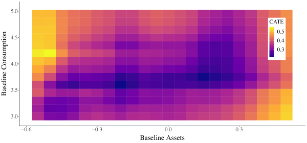
We now return to the application to the data studied in Banerjee et al., (2015), considered in Section 1. Figure 2 displays upper and lower confidence bounds for the CATE (1.2) on post-treatment assets. These bounds are built with the confidence region formulated in 2.1.
Consistent with the qualitative features of the estimates displayed in Figure 1, the null hypothesis that the CATE is equal to zero is only rejected for individuals with low baseline assets and high baseline consumption. That is, the graduation program has a positive impact on individuals who do not have many assets to begin with, but who do have access to a stable source of consumption. On the other hand, the confidence regions contain zero for individuals who have either low baseline consumption or high baseline assets.
| Panel A: Upper Bound |
 |
| Panel B: Lower Bound |
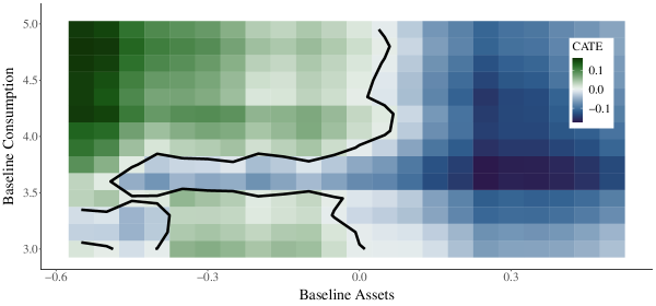 |
Notes: Figure 2 displays heat maps giving half-sample upper and lower confidence bounds for the CATE of the intervention studied in Banerjee et al., (2015) on post-treatment total assets. The confidence bounds are constructed at level . The upper and lower bounds are displayed with different color palettes to emphasize the use of different scales. A contour line has been superimposed over the lower bound to demarcate where the bound crosses zero. The axes and estimator are the same as in Figure 1.
It is illustrative to contrast the estimates and confidence bounds displayed in Figures 1 and 2 with a more frequently encountered method for assessing treatment effect heterogeneity—interacted linear regression. Table 1 reports estimates and standard errors associated with several linear regression specifications, constructed with the same data. The first column reports the coefficient from a regression of post-treatment assets on a treatment indicator. Consistent with results reported in Banerjee et al., (2015), the average effect of the program is positive and significant. The second and third specifications interact the treatment indicator with pre-treatment assets and consumption, respectively. In both cases, the estimate of the coefficient on the interaction is statistically insignificant. The fourth specification interacts both pre-treatment assets and consumption with a treatment indicator. Here, all coefficients lose statistical significance.
The implicit view of much of applied economics appears to be that the flexibility afforded by nonparametric methods is not worth sacrificing the statistical precision of more parsimonious, linear, alternatives.111111We conduct a small survey of papers published in the American Economic Review in the first six months of 2023. Of 38 empirical papers, 30 assess treatment effect heterogeneity in some way. As best as we can tell, only two papers display nonparametric estimates of effect heterogeneity. By contrast, 10 display the results of an interacted linear regression typified by Table 1. The rest are either structural papers, or are only interested in interactions with binary covariates. See Section D.1 for more details. The exercise here suggests otherwise. The linearity imposed by interacted regression masks the structure in the effect heterogeneity recovered by the GRF estimator. The resulting bias is so substantial that statistical significance is lost. The half-sample confidence regions developed in this paper enable the recovery of statistically significant measurements of effect heterogeneity. The remainder of the paper is devoted to developing theoretical guarantees on the accuracy of confidence bounds typified by Figure 2.
| Dependent Variable: Post-Treatment Assets | ||||
| (1) | (2) | (3) | (4) | |
| Treatment | 0.218 (0.031) | 0.194 (0.032) | 0.102 (0.172) | 0.111 (0.201) |
| Assets | 0.770 (0.051) | 1.229 (0.288) | ||
| Consumption | 0.06 (0.022) | -0.026 (0.026) | ||
| Assets Consumption | -0.119 (0.076) | |||
| Treatment Assets | 0.047 (0.093) | -0.065 (0.552) | ||
| Treatment Consumption | 0.031 (0.045) | 0.021 (0.050) | ||
| Treatment Assets Consumption | 0.027 (0.141) | |||
| Observations: | 2,438 | 2,438 | 2,438 | 2,438 |
3. Subsampled Kernel Regression
We establish a bound on the accuracy of the nominal coverage probability for the confidence region introduced in 2.1. We begin in Section 3.1 by discussing subsampled kernel regression and introducing several quantities that take a prominent role in our analysis. Our results apply to conditional moments that satisfy a Neyman orthogonality condition, in addition to several simple regularity conditions. We overview these restrictions in Section 3.2. Our main result is stated in Section 3.3. The results of a simulation calibrated to the Banerjee et al., (2015) data are reported in Section 3.4.
3.1. Subsampled Kernel Regression
Subsampled kernel regression is a broad class of algorithms for solving regression problems of the form (1.5), based on constructing a data-driven kernel function with subsampling. Formally, fix some positive integer and let collect a sequence of subsets of drawn independently and uniformly from . Let denote some auxiliary source of randomness and let collect a set of independent random variables with the same distribution as . We study conditional empirical moment estimators of the form (1.5), where the kernel function admits the decomposition
| (3.1) |
for some known kernel . Several widely applied instances of subsampled kernels are as follows.
Example 3.1 (Subsampled -Nearest Neighbor Regression).
Example 3.2 (Random Forest Regression).
Random forest regression, introduced by Breiman, (2001), is another example of a kernel with the structure (3.1). In this case, each pair generates some partition of the domain of . The kernel is non-zero if and only if and are in the same element of the partition generated by . Often, such partitions are constructed with recursive algorithms, e.g., the “CART” algorithm of Breiman et al., (1984).
We impose the following restrictions on the kernels under consideration.
Assumption 3.1 (Honesty and Symmetry).
(i) The kernel is Honest in the sense that
| (3.2) |
where denotes conditional independence and denotes the set .
(ii) The kernel is positive and satisfies the restriction almost surely. Moreover, the conditional expectation is invariant to permutations of the data .
The “Honesty” condition stipulated in Part (i) of Assumption 3.1 imposes the restriction that any part of the data that can affect the value of the moment cannot affect the value of the kernel . This condition was introduced in Athey and Imbens, (2016). Honesty is often achieved through kernel construction schemes based on sample-splitting; see Wager and Athey, (2018) and Athey et al., (2019) for further discussion. Part (i) of Assumption 3.1 imposes several weak regularity conditions.
The following two quantities restrict the “size” and “variability” of the chosen kernel.
Definition 3.1 (Shrinkage and Incrementality).
(i) We say that the kernel has a uniform shrinkage rate if
| (3.3) |
(ii) We say that a kernel is uniformly incremental if
| (3.4) |
where is an independent random variable with distribution .
The shrinkage rate of a kernel is analogous to the bandwidth of a classical, deterministic, kernel. The incrementality restriction ensures that the chosen kernel is not overly dependent on a single data point. Both notions were introduced by Wager and Athey, (2018) and have been characterized explicitly for various widely applied subsampled kernel estimators.121212The terminology “shrinkage” was introduced in Oprescu et al., (2019), and is not intended to connote (explicit) regularization.
Example 3.3 (continues=ex: knn).
In the case of honest subsampled -NN regression, Khosravi et al., (2019) show that , where is the “intrinsic dimension” of the measure of the covariates . Roughly speaking, a distribution has an intrinsic dimension of if it is (locally) well approximated by a measure supported on a subspace of of dimension . See e.g., Kpotufe, (2011) for further discussion. In turn, Khosravi et al., (2019) and Peng et al., (2022) show that the kernels associated with both honest and non-honest variants of -NN regression are incremental, up to logarithmic factors that depend on the dimension of the covariates.
Example 3.4 (continues=ex: random forest).
Analogously, for honest random forest regression, Wager and Athey, (2018) establish that , where is the dimension of the domain of . See e.g., Wager and Athey, (2018) and Oprescu et al., (2019) for further discussion. Bounds adaptive to the intrinsic dimension of the measure of are given in Huo et al., (2023) under further restrictions. Wager and Athey, (2018) and Peng et al., (2022) give simple conditions under which the kernel associated with subsampled, honest, random forest regression is uniformly incremental, again up to dimension dependent logarithmic factors.
3.2. Moment Restrictions
The uniform confidence region introduced in 2.1 is based on undersmoothing, in the sense that the construction makes no explicit correction for bias. In other words, the confidence regions that we consider are reliant on the use of estimators whose bias is of a smaller stochastic order than the sampling variance. To this end, we emphasize the use of conditional moments , that satisfy a local Neyman Orthogonality condition.
Definition 3.2 (Local Neyman Orthogonality).
We say that a conditional moment is uniformly locally Neyman orthogonal if
| (3.5) |
for all in and in .
The use of Neyman orthogonal moments ensures that the bias induced by the estimation of the nuisance parameter with is small (Newey,, 1994).
In addition to Neyman orthogonality, we require several smoothness restrictions on the function . In the main text, to ease exposition, we impose the following linearity and boundedness restriction.
Assumption 3.2 (Moment Linearity and Boundedness).
The moment function satisfies the linear representation
| (3.6) |
for some known functions and . Moreover, the absolute value of the function is bounded by the constant almost surely.
The linearity restriction entailed in Assumption 3.2 is inessential and is imposed for the sake of simplicity.131313In Appendix A, we show that moment linearity can be replaced by the high-level assumption that is consistent for . This state of affairs is standard in -estimation problems (see e.g., Newey and McFadden,, 1994). As our running examples use linear moments, and sufficient conditions for the consistency of have been established (see e.g., Assumption 4.1 and Theorem 4.3 of Oprescu et al.,, 2019), we omit a detailed consideration of nonlinear moments. The boundedness restriction is easily weakened to a slightly more involved assumption stated in terms of the sub-exponential norm. Again, we impose boundedness to ease exposition.
We maintain the following mild smoothness restrictions on the moment function .
Assumption 3.3 (Moment Smoothness).
(i) The moment is second order smooth, in the sense that
| (3.7) |
for each in .
(ii) The variogram
is uniformly Lipschitz in both of its components, in the sense that
| (3.8) |
holds for all and in and
| (3.9) |
holds for each and in .
(iii) Define the moments
associated with the functions and introduced in Assumption 3.2. Both moments are uniformly Lipschitz in their first component, in the sense that
| (3.10) |
for each in and all and in . Moreover, the first moment is uniformly Lipschitz in its third component and bounded from below in the sense that
| (3.11) | ||||
| (3.12) |
for each in and some positive constant .
Neyman orthogonal moments satisfying the smoothness restrictions specified in Assumptions 3.2 and 3.3 are available for many widely considered statistical problems.
Example 3.5 (Nonparametric Regression).
Suppose that contains a measurement of an outcome and a vector of covariates and that the data are some function, e.g., a sub-vector, of . In this setting, we are often interested in estimating the conditional expectation function
Here, the parameter is identified via the linear moment function . As there are no nuisance parameters, local Neyman orthogonality is immediate.
Example 3.6 (Conditional Average Treatment Effects).
Now, suppose that additionally contains a binary valued variable that indicates whether unit has been randomly assigned to an intervention. In this case, interest may be in estimating a CATE (1.2). Under strong ignorability, the CATE is identified by several moment functions, e.g., those implied by inverse propensity weighting or outcome regression (Imbens and Rubin,, 2015). The moment (1.3) is the unique Neyman orthogonal identifying moment for the parameter (1.2) (see e.g., Hahn,, 1998; Chernozhukov et al.,, 2018). Note that, in this case, Part (i) of Assumption 3.3 is implied by the more refined bound
| (3.13) |
where and are defined in (1.4). This structure yields the celebrated “Double Robustness” result for estimation of average treatment effects and conditional average treatment effects; see Chernozhukov et al., (2018) and Kennedy, (2023) for further discussion. We impose the more general condition (3.7), as this bound exhibits many of the same features and will hold for a wider variety of problems.
Example 3.7 (Conditional Local Average Treatment Effects).
In turn, suppose that additionally contains a measurement of a binary instrument and that interest is now in estimating the conditional local average treatment effect
| (3.14) |
where and are the potential outcomes for the treatment generated by the instrument . Under standard assumptions (Angrist et al.,, 1996), Tan, (2006) and Frölich, (2007) show that the unique Neyman orthogonal moment function for the parameter (3.14) is given by
| (3.15) |
where the nuisance parameter now collects the nuisance functions
| (3.16) |
and denotes the instrumental propensity score.
Additional examples of problems where smooth Neyman orthogonal identifying moments are available include estimation of partially linear regression and partially linear instrumental variable regression (Chernozhukov et al.,, 2018), dynamic treatment effects (Lewis and Syrgkanis,, 2021), and long-term treatment effects identified by surrogate outcomes (Athey et al.,, 2020; Chen and Ritzwoller,, 2023). Ichimura and Newey, (2022) and Belloni et al., (2018) provide extensive discussion on the derivation of Neyman orthogonal moments. Further discussion of the role of Neyman orthogonality in semiparametric estimation is given in Chernozhukov et al., (2018) and Foster and Syrgkanis, (2023).
3.3. Coverage
The following theorem gives a bound on the error in the nominal coverage probability of the confidence regions introduced in 2.1. We emphasize that the result is applicable to asymptotic regimes where the dimension of the query-vector can be exponentially larger than the sample size .
Theorem 3.1 (Coverage Error Bound).
Suppose that the kernel satisfies Assumption 3.1, has uniform shrinkage rate , and is uniformly incremental and that the Neyman orthogonal moment function satisfies Assumptions 3.2 and 3.3. Moreover, suppose that quantity is uniformly bounded as varies over and that has been chosen to satisfy . If the nuisance parameter estimator satisfies the probability bound
| (3.17) |
for some sequence , then the confidence region formulated in 2.1 satisfies the bound
| (3.18) |
for all sufficiently large and .141414The statistical family is defined implicitly by the omitted constants in the uniform bounds stated in 3.1 and Assumption 3.3, in addition to the restriction that is bounded as varies over .
Remark 3.1.
Theorem 3.1 follows from an application of a more general result stated in Appendix A. This result applies to conditional moment estimators that are not necessarily constructed with subsampled kernels. Rather, the result holds under the high-level assumption that the estimator is approximately linear, with a sufficiently small remainder term, and has sufficiently small bias and stochastic equicontinuity. These conditions are verified for subsampled kernel regression in Appendix B.
Several aspects of this argument are new. In particular, through a standard series of expansions (see e.g., Chernozhukov et al.,, 2018), we show that the root is approximated by
| (3.19) | ||||
with a remainder term given by the second term in (3.18). The quantity (3.19) can be recognized as a complete, deterministic, -statistic of order .151515The incrementality condition specified in 3.1 ensures that this -statistic is non-degenerate. We then apply a new result that demonstrates that -statistics of order are approximately linear with a remainder term of order , up to logarithmic factors. This is a dramatic improvement over analogous results given in Song et al., (2019) and Minsker, (2023), whose remainder terms exhibit polynomial decay as and grow and only apply to regime . This regime is unsuitable for our application. This result has other applications and is discussed in detail in Section 4.
In other words, we establish that the root satisfies a linear representation of the form (2.6) up to a small remainder term. It immediately follows that the bootstrap root satisfies the linear representation (2.7), up to a small remainder term, as it is constructed with subsampling. We conclude by applying suitable high-dimensional central limit theorems (Chernozhuokov et al.,, 2022) to the linear terms (2.6) and (2.7). To handle the half-sample bootstrap, we apply an argument, based on a coupling proposed in Yadlowsky et al., (2023), similar to the Poissonization trick used in Præstgaard and Wellner, (1993).
Remark 3.2.
Remark 3.3.
It is worth emphasizing that the coverage bound given in Theorem 3.1 is achieved without assuming that the estimator is constructed with sample-splitting. That is, the nuisance parameter estimator can be computed using the same data used to evaluate the conditional moment . Often, sample-splitting is necessary to ensure that stochastic equicontinuity is sufficiently small (Chernozhukov et al.,, 2018). Avoiding sample-splitting can be practically important; Ritzwoller and Romano, (2023) show that the randomness induced by sample-splitting can be large.
Theorem 3.1 states a bound on coverage error in terms of two generic sequences: , expressing the rate of convergence of the nuisance parameter estimator , and , measuring the effective bandwidth of the kernel. The bound (3.18) exhibits an interesting tradeoff between these objects and the choice of subsample size . To see this, suppose that
| (3.20) |
with probability greater than , for some constants , , and between and . In this case, ignoring logarithmic factors and other constants, the bound (3.18) can be re-expressed as
| (3.21) |
In other words, the confidence region defined in 2.1 is consistent if
| (3.22) |
respectively. That is, we are able to accommodate larger values of the shrinkage rate and nuisance parameter estimation error if the subsample size is larger, relative to the sample size . However, as the subsample size increases, the normal approximation error (i.e., the first term in (3.18)) increases.
Recall from Section 3.1 that, for many popular, honest, subsampled kernel estimators, the shrinkage rate satisfies a bound for some small constant and some integer measuring the (potentially, intrinsic) dimension of the covariates . Thus, in order to ensure that the second inequality in consistency condition (3.22) is satisfied, it is essential to accommodate subsample sizes close to one, i.e., the regime . This is enabled by the general results on the asymptotic linearity of -statistics given in Section 4.
On the other hand, when the subsample size scaling factor is close to one, the restriction imposed by the consistency condition (3.22) on the rate of convergence of the nuisance parameter estimator is very weak. Observe that the case implies the familiar condition that nuisance parameters can be estimated at the rate in root mean squared error (Chernozhukov et al.,, 2018). If the nuisance parameter estimator is itself estimated with random forest regression, Syrgkanis and Zampetakis, (2020), Chi et al., (2022), and Huo et al., (2023), among others, give conditions under which sufficient rates of convergence can be achieved.
3.4. Performance
We now measure the performance of the confidence region formulated in 2.1. We apply a method for simulation design proposed by Athey et al., (2021). In particular, we calibrate a simulation to the Banerjee et al., (2015) data using a Generative Adversarial Network (GAN) (Goodfellow et al.,, 2014). Further details on this calibration are given in Appendix E. In effect, we construct a data generating process that approximates the Banerjee et al., (2015) data, where we know the true value of the CATE queried at each value used to construct the grids displayed in Figures 1 and 2.
Measurements are taken as two parameters vary. First, we consider several values of the sample size . In particular, we consider settings with , for in , where is the sample size of the Banerjee et al., (2015) data. Second, we vary the proportion . We consider three regimes: , , and . Observe that increases in proportion to in the first regime and that is constant as varies in the third regime.161616We choose the same value of for constructing the empirical moment and the nuisance parameter estimator . The second regime resides between these two extremes.
Figure 3 displays measurements of the coverage and width of the confidence region formulated in 2.1, in addition to measurements of the bias of the estimator . The first row displays measurements of the coverage of the confidence region, the coverage of the lower bound (i.e., Panel B of Figure 2), and the coverage of the upper bound (i.e., Panel A of Figure 2). The nominal level is . At the observed sample size , i.e., , the confidence region is somewhat anti-conservative. Consistent with the structure of the bound (3.18), coverage does not improve as the sample size increases unless the proportion also decreases. In the regimes where the proportion decreases as the sample multiplier increases, coverage becomes moderately conservative.
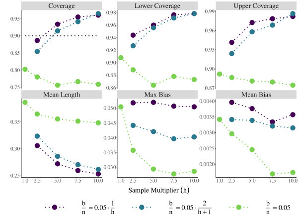 |
Notes: Figure 3 displays several measurements of the performance of the confidence intervals formulated in 2.1 in a simulation calibrated to the Banerjee et al., (2015) data. The nominal level is ; a horizontal dotted line is displayed at the nominal coverage in the first panel. The confidence bounds considered are constructed analogously to the confidence bounds displayed in Figure 2. The -axis of each panel is the sample multiplier . The color of each measurement varies with the choice of . Further details on this design and implementation of this simulation are given in Appendix E.
The second row of Figure 3 illustrates a bias-variance trade-off with the subsample size . The first panel displays measurements of the average width of the confidence region. Here, the average is taken over both simulation draws and the query-vector . The width of the confidence region is increasing in the proportion and is essentially constant if is constant as increases. By contrast, the second two panels display the maximum and average bias of the estimator , again taken over the query-vector . The bias is decreasing in the proportion and is essentially constant if is constant as varies.171717The default value for the proportion in the GRF R package is . The results of this simulation suggest that this proportion should be reduced, at least in settings where the dimension of the covariate vector is small.
4. General Results for High-Dimensional -Statistics
An essential step in the proof of Theorem 3.1 follows from a new order-explicit bound on the remainder in a linear approximation to a high-dimensional -statistic. In this section, we present this result and state several corollaries. In particular, we give new order-explicit results on the concentration and normal approximation of high-dimensional -statistics. That is, we consider the asymptotic behavior of the order -statistic
| (4.1) |
where the vector collects the deterministic, symmetric, real-valued kernel function evaluated at the -vector of points in the space . We assume that each component of the kernel function has mean zero. Proofs for results stated in this section are given in Appendix C.
4.1. Context
The asymptotic analysis of -statistics was initiated by Hoeffding, (1948), who established a central limit theorem in the regime where the order is fixed and the sample size is increasing. The Hoeffding central limit theorem has been extended only recently to the regime where the order increases with the sample size . DiCiccio and Romano, (2022) give a result with this flavor in the regime where . Wager and Athey, (2018), Peng et al., (2022), and Minsker, (2023) are able to strengthen this result to the regime where . We state and prove this more general result for the sake of completeness, and because its main ideas will serve as useful touch points in the more involved analysis to follow. We use an argument similar to the proof of Theorem 3.1 of Minsker, (2023). Define the kernel variance , the Hájek projection
| (4.2) |
and the Hájek projection variance .
Theorem 4.1 (Hoeffding Central Limit Theorem).
For any sequence of kernel orders , where
| (4.3) |
as , we have that
| (4.4) |
as , where denotes convergence in distribution.
Remark 4.1.
Theorem 4.1 is established by considering the decomposition
| (4.5) |
In particular, we give a high-probability bound for the second term and apply a standard central limit theorem to the first term. The condition (4.3) is needed to bound the second term. As a by-product of the proof, we show that . Thus, the normalization (4.3) implies that .
Large deviation bounds for high-dimensional -statistics, i.e., -statistics with vector-valued kernels, were not given until Hoeffding, (1963). This result is now more standard; a modern version is stated as follows. A proof is given in Song et al., (2019). The norm denotes the -Orlicz norm.181818Random variables are sub-Exponential if and only if they have a finite -Orlicz norm (Section 2.7, Vershynin,, 2018).
Lemma 4.1 (Lemma A.5, Song et al., (2019)).
If the -Orlicz norm bound
| (4.6) |
is satisfied for each in , then
| (4.7) |
with probability greater than , where .
Again, Lemma 4.1 demonstrates that concentrates in the regime that , up to a logarithmic factor that depends on the dimension . Here, however, concentration is expressed in terms of the quantity , rather than the more appropriate, and potentially substantively smaller, normalizing quantity used in Theorem 4.1. In part motivated by this incongruity, Arcones and Giné, (1993), Arcones, (1995), Giné et al., (2000), establish a series of refined large deviation bounds for high-dimensional -statistics that use the appropriate normalizing factor (among many other related results). See De la Pena and Giné, (1999) for a textbook treatment. However, the constants used to express these bounds depend implicitly on the order , and so are not applicable to asymptotic regimes where may be growing with the sample size .
More recently, Chen, (2018), Chen and Kato, (2019), and Song et al., (2019) have studied central limit theorems for high-dimensional -statistics. Of these papers, only Song et al., (2019) gives results with explicit dependence on the order . Their results are only applicable to the regime where . Minsker, (2023) gives a large deviation bound with the correct normalizing factor and explicit order dependence, but this result is again only applicable to the regime .
4.2. Concentration of the Hájek Residual
We obtain a large deviation bound on the difference
| (4.8) |
We refer to the quantity (4.8) as the Hájek residual (Hájek,, 1968). This bound is used in the proof of Theorem 3.1 and implies a new large deviation bound and central limit theorem for high-dimensional -statistics, stated in the following subsection.
Theorem 4.2.
Define the terms
| (4.9) |
If the kernel function satisfies the bound (4.6) for each in , then
| (4.10) | |||
with probability greater than .
Remark 4.2.
Roughly speaking, the bound (4.10) follows by first demonstrating that the Hájek residual can be expressed as a degenerate -statistic of order . This allows us to derive Hoffman-Jørgensen type bounds on higher moments of (4.8) with a symmetrization argument. Here, we make essential use of a symmetrization inequality for completely degenerate kernels, with explicit dependence on the order, due to Sherman, (1994). This symmetrization inequality was also used in Song et al., (2019) and Minsker, (2023).
Remark 4.3.
The bound (4.10) implies that if for some positive constant , then the Hájek residual is (roughly) of stochastic order for all sufficiently large . This is a dramatic improvement over existing bounds (Song et al.,, 2019; Minsker,, 2023), which decay polynomially as and increase and only converge to zero in the regime . In our view, this result hints at an explanation for the widespread success of subsampling in machine learning and statistical inference. Subsampled statistics, of a large order, are essentially linear.
4.3. Concentration and Normal Approximation
We now state a large deviation bound and central limit theorem for the high-dimensional -statistic (4.1). Both results are corollaries of Theorem 4.2, apply to the regime , and depend on the correct normalizing factor.
Corollary 4.1.
Let be the diagonal matrix with components .
(ii) Let denote a centered Gaussian random vector with covariance matrix . Under the same conditions as Theorem 4.2, we have that
| (4.12) |
where denotes the set of hyper-rectangles in .
Remark 4.4.
De la Pena and Giné, (1999) state a result analogous to Part (i) of 4.1, in the sense that the -statistic is normalized by the correct quantity . The constants used in their bound depend implicitly on . Part (i) of 4.1 improves substantially on Lemma 4.1 in contexts where the Hájek projection variances are smaller than .191919Section 4 of Song et al., (2019) gives several examples of statistics where the Hájek projection variance is smaller than . Under the restriction , imposed in the application to subsampled kernel regression considered in Section 3, Part (i) of 4.1 only improves on Lemma 4.1 by a constant factor. Part (ii) of 4.1 gives a high-dimensional equivalent to Theorem 4.1. An analogous half-sample bootstrap central limit theorem follows from arguments very similar to parts of the proof of Theorem 3.1.
5. Conclusion
We propose a confidence region for solutions to conditional moment equations. The confidence region is built around an estimator based on subsampled kernel regression. As a running example, we consider the construction of confidence regions for conditional average treatment effects around a Generalized Random Forest (Athey et al.,, 2019). Empirically, we document that the proposed confidence region is able to recover treatment effect heterogeneity undetected by interacted linear regression. Theoretically, we establish a bound on coverage accuracy that illustrates a bias-variance tradeoff in the user-chosen subsample size. In order to do this, we obtain several new results on the asymptotics of high-dimensional -statistics.
We give conditions sufficient for the asymptotic validity of the proposed confidence regions. However, the confidence region is not necessarily optimal, in any particular sense, under the maintained assumptions. It is likely to be the case an optimal confidence region would need to incorporate a bias estimate and procedure for choosing tuning parameters to balance bias and variance (see e.g., Chernozhukov et al., (2014), Chen et al., (2024) for instantiations of these ideas). Adapting this approach to subsampled moment regression is an interesting direction for further research.
References
- Adler and Taylor, (2009) Adler, R. J. and Taylor, J. E. (2009). Random fields and geometry. Springer Science & Business Media.
- Ai and Chen, (2003) Ai, C. and Chen, X. (2003). Efficient estimation of models with conditional moment restrictions containing unknown functions. Econometrica, 71(6):1795–1843.
- Angrist et al., (1996) Angrist, J. D., Imbens, G. W., and Rubin, D. B. (1996). Identification of causal effects using instrumental variables. Journal of the American statistical Association, 91(434):444–455.
- Arcones, (1995) Arcones, M. A. (1995). A bernstein-type inequality for u-statistics and u-processes. Statistics & probability letters, 22(3):239–247.
- Arcones and Giné, (1993) Arcones, M. A. and Giné, E. (1993). Limit theorems for u-processes. The Annals of Probability, pages 1494–1542.
- Armstrong and Kolesár, (2020) Armstrong, T. B. and Kolesár, M. (2020). Simple and honest confidence intervals in nonparametric regression. Quantitative Economics, 11(1):1–39.
- Athey et al., (2020) Athey, S., Chetty, R., Imbens, G., and Kang, H. (2020). Estimating treatment effects using multiple surrogates: The role of the surrogate score and the surrogate index.
- Athey and Imbens, (2016) Athey, S. and Imbens, G. (2016). Recursive partitioning for heterogeneous causal effects. Proceedings of the National Academy of Sciences, 113(27):7353–7360.
- Athey et al., (2021) Athey, S., Imbens, G. W., Metzger, J., and Munro, E. (2021). Using wasserstein generative adversarial networks for the design of monte carlo simulations. Journal of Econometrics.
- Athey et al., (2019) Athey, S., Tibshirani, J., and Wager, S. (2019). Generalized random forests. The Annals of Statistics, 47(2):1148–1178.
- Balboni et al., (2022) Balboni, C., Bandiera, O., Burgess, R., Ghatak, M., and Heil, A. (2022). Why do people stay poor? The Quarterly Journal of Economics, 137(2):785–844.
- Banerjee et al., (2015) Banerjee, A., Duflo, E., Goldberg, N., Karlan, D., Osei, R., Parienté, W., Shapiro, J., Thuysbaert, B., and Udry, C. (2015). A multifaceted program causes lasting progress for the very poor: Evidence from six countries. Science, 348(6236):1260799.
- Belloni et al., (2018) Belloni, A., Chernozhukov, V., Chetverikov, D., and Wei, Y. (2018). Uniformly valid post-regularization confidence regions for many functional parameters in z-estimation framework. Annals of statistics, 46(6B):3643.
- Biau et al., (2008) Biau, G., Devroye, L., and Lugosi, G. (2008). Consistency of random forests and other averaging classifiers. Journal of Machine Learning Research, 9(9).
- Boucheron et al., (2013) Boucheron, S., Lugosi, G., and Massart, P. (2013). Concentration inequalities: A nonasymptotic theory of independence,(2013).
- Breiman, (1996) Breiman, L. (1996). Bagging predictors. Machine learning, 24:123–140.
- Breiman, (2001) Breiman, L. (2001). Random forests. Machine learning, 45:5–32.
- Breiman et al., (1984) Breiman, L., Friedman, J., Olshen, R., and Stone, C. J. (1984). Classification and regression trees. Routledge.
- Bühlmann and Yu, (2002) Bühlmann, P. and Yu, B. (2002). Analyzing bagging. The annals of Statistics, 30(4):927–961.
- Cattaneo et al., (2024) Cattaneo, M. D., Klusowski, J. M., and Tian, P. M. (2024). On the pointwise behavior of recursive partitioning and its implications for heterogeneous causal effect estimation.
- Chen and Ritzwoller, (2023) Chen, J. and Ritzwoller, D. M. (2023). Semiparametric estimation of long-term treatment effects. Journal of Econometrics, 237(2):105545.
- Chen, (2018) Chen, X. (2018). Gaussian and bootstrap approximations for high-dimensional u-statistics and their applications.
- Chen et al., (2024) Chen, X., Christensen, T., and Kankanala, S. (2024). Adaptive estimation and uniform confidence bands for nonparametric structural functions and elasticities. The Review of Economic Studies.
- Chen and Christensen, (2018) Chen, X. and Christensen, T. M. (2018). Optimal sup-norm rates and uniform inference on nonlinear functionals of nonparametric iv regression: Nonlinear functionals of nonparametric iv. Quantitative Economics, 9(1):39–84.
- Chen and Kato, (2019) Chen, X. and Kato, K. (2019). Randomized incomplete -statistics in high dimensions. The Annals of Statistics, 47(6):3127 – 3156.
- Chen and Pouzo, (2012) Chen, X. and Pouzo, D. (2012). Estimation of nonparametric conditional moment models with possibly nonsmooth generalized residuals. Econometrica, 80(1):277–321.
- Chernozhukov et al., (2018) Chernozhukov, V., Chetverikov, D., Demirer, M., Duflo, E., Hansen, C., Newey, W., and Robins, J. (2018). Double/debiased machine learning for treatment and structural parameters: Double/debiased machine learning. The Econometrics Journal, 21(1).
- Chernozhukov et al., (2013) Chernozhukov, V., Chetverikov, D., and Kato, K. (2013). Gaussian approximations and multiplier bootstrap for maxima of sums of high-dimensional random vectors.
- Chernozhukov et al., (2014) Chernozhukov, V., Chetverikov, D., and Kato, K. (2014). Anti-concentration and honest, adaptive confidence bands. The Annals of Statistics, 42(5):1787–1818.
- (30) Chernozhukov, V., Chetverikov, D., and Kato, K. (2017a). Central limit theorems and bootstrap in high dimensions. The Annals of Probability, 45(4):2309 – 2352.
- (31) Chernozhukov, V., Chetverikov, D., and Kato, K. (2017b). Detailed proof of nazarov’s inequality. arXiv preprint arXiv:1711.10696.
- Chernozhukov et al., (2022) Chernozhukov, V., Escanciano, J. C., Ichimura, H., Newey, W. K., and Robins, J. M. (2022). Locally robust semiparametric estimation. Econometrica, 90(4):1501–1535.
- Chernozhukov et al., (2023) Chernozhukov, V., Newey, W. K., and Santos, A. (2023). Constrained conditional moment restriction models. Econometrica, 91(2):709–736.
- Chernozhuokov et al., (2022) Chernozhuokov, V., Chetverikov, D., Kato, K., and Koike, Y. (2022). Improved central limit theorem and bootstrap approximations in high dimensions. The Annals of Statistics, 50(5):2562–2586.
- Chi et al., (2022) Chi, C.-M., Vossler, P., Fan, Y., and Lv, J. (2022). Asymptotic properties of high-dimensional random forests. The Annals of Statistics, 50(6):3415–3438.
- Chung and Romano, (2013) Chung, E. and Romano, J. P. (2013). Exact and asymptotically robust permutation tests. The Annals of Statistics, 41(2):484–507.
- De la Pena and Giné, (1999) De la Pena, V. and Giné, E. (1999). Decoupling: from dependence to independence. Springer.
- DiCiccio and Romano, (2022) DiCiccio, C. and Romano, J. (2022). Clt for u-statistics with growing dimension. Statistica Sinica, 32(1).
- Efron and Stein, (1981) Efron, B. and Stein, C. (1981). The jackknife estimate of variance. The Annals of Statistics, pages 586–596.
- Fix and Hodges, (1989) Fix, E. and Hodges, J. L. (1989). Discriminatory analysis. nonparametric discrimination: Consistency properties. International Statistical Review/Revue Internationale de Statistique, 57(3):238–247.
- Foster and Syrgkanis, (2023) Foster, D. J. and Syrgkanis, V. (2023). Orthogonal statistical learning. The Annals of Statistics, 51(3):879–908.
- Frölich, (2007) Frölich, M. (2007). Nonparametric iv estimation of local average treatment effects with covariates. Journal of Econometrics, 139(1):35–75.
- Giné et al., (2000) Giné, E., Latała, R., and Zinn, J. (2000). Exponential and moment inequalities for u-statistics. In High Dimensional Probability II, pages 13–38. Springer.
- Goodfellow et al., (2014) Goodfellow, I., Pouget-Abadie, J., Mirza, M., Xu, B., Warde-Farley, D., Ozair, S., Courville, A., and Bengio, Y. (2014). Generative adversarial nets. Advances in neural information processing systems, 27.
- Götze et al., (2021) Götze, F., Sambale, H., and Sinulis, A. (2021). Concentration inequalities for polynomials in -sub-exponential random variables. Electronic Journal of Probability, 26(none):1 – 22.
- Hahn, (1998) Hahn, J. (1998). On the role of the propensity score in efficient semiparametric estimation of average treatment effects. Econometrica, pages 315–331.
- Hájek, (1968) Hájek, J. (1968). Asymptotic normality of simple linear rank statistics under alternatives. The Annals of Mathematical Statistics, pages 325–346.
- Hanson and Wright, (1971) Hanson, D. L. and Wright, F. T. (1971). A bound on tail probabilities for quadratic forms in independent random variables. The Annals of Mathematical Statistics, 42(3):1079–1083.
- Hoeffding, (1948) Hoeffding, W. (1948). A class of statistics with asymptotically normal distribution. Ann. Math. Statist., 19(4):293–325.
- Hoeffding, (1963) Hoeffding, W. (1963). Probability inequalities for sums of bounded random variables. Journal of the American Statistical Association, pages 13–30.
- Huo et al., (2023) Huo, Y., Fan, Y., and Han, F. (2023). On the adaptation of causal forests to manifold data. arXiv preprint arXiv:2311.16486.
- Ichimura and Newey, (2022) Ichimura, H. and Newey, W. K. (2022). The influence function of semiparametric estimators. Quantitative Economics, 13(1):29–61.
- Imbens and Rubin, (2015) Imbens, G. W. and Rubin, D. B. (2015). Causal inference in statistics, social, and biomedical sciences. Cambridge University Press.
- Kennedy, (2023) Kennedy, E. H. (2023). Towards optimal doubly robust estimation of heterogeneous causal effects. Electronic Journal of Statistics, 17(2):3008–3049.
- Khosravi et al., (2019) Khosravi, K., Lewis, G., and Syrgkanis, V. (2019). Non-parametric inference adaptive to intrinsic dimension. arXiv preprint arXiv:1901.03719.
- Kpotufe, (2011) Kpotufe, S. (2011). k-nn regression adapts to local intrinsic dimension. Advances in neural information processing systems, 24.
- Kraay and McKenzie, (2014) Kraay, A. and McKenzie, D. (2014). Do poverty traps exist? assessing the evidence. Journal of Economic Perspectives, 28(3):127–148.
- Kuchibhotla et al., (2023) Kuchibhotla, A. K., Balakrishnan, S., and Wasserman, L. (2023). Median regularity and honest inference. Biometrika, 110(3):831–838.
- Lee, (1990) Lee, A. (1990). U-statistics: theory and practice. Taylor & Francis.
- Lewis and Syrgkanis, (2021) Lewis, G. and Syrgkanis, V. (2021). Double/debiased machine learning for dynamic treatment effects. In NeurIPS, pages 22695–22707.
- Li, (1989) Li, K.-C. (1989). Honest confidence regions for nonparametric regression. The Annals of Statistics, 17(3):1001–1008.
- Lin and Jeon, (2006) Lin, Y. and Jeon, Y. (2006). Random forests and adaptive nearest neighbors. Journal of the American Statistical Association, 101(474):578–590.
- Mentch and Hooker, (2014) Mentch, L. and Hooker, G. (2014). Ensemble trees and clts: Statistical inference for supervised learning. stat, 1050:25.
- Mentch and Hooker, (2016) Mentch, L. and Hooker, G. (2016). Quantifying uncertainty in random forests via confidence intervals and hypothesis tests. The Journal of Machine Learning Research, 17(1):841–881.
- Minsker, (2023) Minsker, S. (2023). U-statistics of growing order and sub-gaussian mean estimators with sharp constants. Mathematical Statistics and Learning.
- Montgomery-Smith, (1993) Montgomery-Smith, S. J. (1993). Comparison of sums of independent identically distributed random variables. Probability and Mathematical Statistics, 14:281–285.
- Newey, (1993) Newey, W. K. (1993). Efficient estimation of models with conditional moment restrictions. In Econometrics, volume 11 of Handbook of Statistics, pages 419–454. Elsevier.
- Newey, (1994) Newey, W. K. (1994). The asymptotic variance of semiparametric estimators. Econometrica: Journal of the Econometric Society, pages 1349–1382.
- Newey and McFadden, (1994) Newey, W. K. and McFadden, D. (1994). Large sample estimation and hypothesis testing. Handbook of econometrics, 4:2111–2245.
- Nie and Wager, (2021) Nie, X. and Wager, S. (2021). Quasi-oracle estimation of heterogeneous treatment effects. Biometrika, 108(2):299–319.
- Oprescu et al., (2019) Oprescu, M., Syrgkanis, V., and Wu, Z. S. (2019). Orthogonal random forest for causal inference. In International Conference on Machine Learning, pages 4932–4941. PMLR.
- Peng et al., (2022) Peng, W., Coleman, T., and Mentch, L. (2022). Rates of convergence for random forests via generalized u-statistics. Electronic Journal of Statistics, 16(1):232–292.
- Politis and Romano, (1994) Politis, D. N. and Romano, J. P. (1994). Large sample confidence regions based on subsamples under minimal assumptions. The Annals of Statistics, pages 2031–2050.
- Politis et al., (1999) Politis, D. N., Romano, J. P., and Wolf, M. (1999). Subsampling. Springer Science & Business Media.
- Præstgaard and Wellner, (1993) Præstgaard, J. and Wellner, J. A. (1993). Exchangeably weighted bootstraps of the general empirical process. The Annals of Probability, pages 2053–2086.
- Ritzwoller and Romano, (2023) Ritzwoller, D. M. and Romano, J. P. (2023). Reproducible aggregation of sample-split statistics. arXiv preprint arXiv:2311.14204.
- Robins et al., (1994) Robins, J. M., Rotnitzky, A., and Zhao, L. P. (1994). Estimation of regression coefficients when some regressors are not always observed. Journal of the American statistical Association, 89(427):846–866.
- Romano and Shaikh, (2012) Romano, J. P. and Shaikh, A. M. (2012). On the uniform asymptotic validity of subsampling and the bootstrap. The Annals of Statistics, 40(6).
- Scornet et al., (2015) Scornet, E., Biau, G., and Vert, J.-P. (2015). Consistency of random forests. Annals of Statistics, 43(4):1716–1741.
- Sexton and Laake, (2009) Sexton, J. and Laake, P. (2009). Standard errors for bagged and random forest estimators. Computational Statistics & Data Analysis, 53(3):801–811.
- Sherman, (1994) Sherman, R. P. (1994). Maximal inequalities for degenerate u-processes with applications to optimization estimators. The Annals of Statistics, 22(1):439–459.
- Singh and Vijaykumar, (2023) Singh, R. and Vijaykumar, S. (2023). Kernel ridge regression inference. arXiv preprint arXiv:2302.06578.
- Song et al., (2019) Song, Y., Chen, X., and Kato, K. (2019). Approximating high-dimensional infinite-order -statistics: Statistical and computational guarantees. Electronic Journal of Statistics, 13(2).
- Syrgkanis and Zampetakis, (2020) Syrgkanis, V. and Zampetakis, M. (2020). Estimation and inference with trees and forests in high dimensions. In Conference on learning theory, pages 3453–3454. PMLR.
- Tan, (2006) Tan, Z. (2006). Regression and weighting methods for causal inference using instrumental variables. Journal of the American Statistical Association, 101(476):1607–1618.
- van der Vaart and Wellner, (2013) van der Vaart, A. W. and Wellner, J. A. (2013). Weak convergence and empirical processes: with applications to statistics. Springer.
- Vershynin, (2018) Vershynin, R. (2018). High-dimensional probability: An introduction with applications in data science, volume 47. Cambridge university press.
- Wager and Athey, (2018) Wager, S. and Athey, S. (2018). Estimation and inference of heterogeneous treatment effects using random forests. Journal of the American Statistical Association, 113(523):1228–1242.
- Wager et al., (2014) Wager, S., Hastie, T., and Efron, B. (2014). Confidence intervals for random forests: The jackknife and the infinitesimal jackknife. The Journal of Machine Learning Research, 15(1):1625–1651.
- Yadlowsky et al., (2023) Yadlowsky, S., Fleming, S., Shah, N., Brunskill, E., and Wager, S. (2023). Evaluating treatment prioritization rules via rank-weighted average treatment effects.
Supplemental Appendix to:
Uniform Inference for Subsampled Moment Regression111Date:
David M. Ritzwoller
Vasilis Syrgkanis
Stanford University
Stanford University
Contents appendix.Asubsection.A.1subsection.A.2subsection.A.3subsection.A.4subsubsection.A.4.1subsubsection.A.4.2subsubsection.A.4.3appendix.Bsubsection.B.1subsubsection.B.1.1subsubsection.B.1.2subsubsection.B.1.3subsubsection.B.1.4appendix.Csubsection.C.1subsection.C.2subsection.C.3subsection.C.4appendix.Dsubsection.D.1subsection.D.2subsubsection.D.2.1subsubsection.D.2.2appendix.Esubsection.E.1subsection.E.2subsection.E.3
Appendix A An Abstract Bound on Coverage Error
In this appendix, we give an abstract bound on the accuracy of the nominal coverage probability for the confidence region introduced in 2.1. That is, we make no use of the kernel structure expressed in (1.5). We specify a set of high-level assumptions in Section A.1. The abstract bound is stated in Section A.2 and proved in Section A.3. Proofs for supporting Lemmas are given in Section A.4.
A.1. Assumptions
We require several mild smoothness restrictions on the moment function . In contrast to the set of assumptions specified in Section 3.2, we do not require moment linearity. Instead, we impose the following generalization of Part (iii) of Assumption 3.3.
Assumption A.1 (Moment Restrictions).
The moment function is twice continuously differentiable in its second argument. Let
| (A.1) |
denote the Jacobian and Hessian of in , respectively. The Jacobian is uniformly Lipschitz in its second argument and bounded from below in the sense that
| (A.2) | ||||
| (A.3) |
for each in and some positive constant . The Hessian is uniformly bounded as , , and vary over their respective domains.
We additionally require Neyman orthogonality and second order smoothness, i.e., Part (i) of Assumption 3.3.
Moreover, we impose an analogous smoothness restriction on the centered empirical moment
| (A.4) |
where we have made the dependence on implicit to ease notation.
Assumption A.2 (Empirical Smoothness).
The centered empirical moment is twice continuously differentiable in its second argument. Let
| (A.5) |
denote the Jacobian and Hessian of in , respectively. The Hessian is uniformly bounded almost surely as , , and vary over their respective domains.
Next, we impose a set of high-level restrictions on the structure of the empirical conditional moment (2.1). At times we refer to the normalized statistic
| (A.6) |
First, we impose a condition that ensures that (A.6) is approximately linear. Recall that the norm denotes the -Orlicz norm.
Assumption A.3 (Approximate Linearity).
There exists a function , a constant , and real-valued sequences and such that ,
| (A.7) |
hold for all in and in . Moreover, if denotes and , then
| (A.8) |
Remark A.1.
Second, we impose several restrictions relating to the estimators and . Throughout, we measure the error in the estimator of in terms of the norm
| (A.9) |
A closely related collection of conditions, in the context of estimation of the solution to unconditional orthogonal moments, is stated as Assumption 3.2 of Chernozhukov et al., (2018).
Assumption A.4 (Bias, Consistency, and Stochastic Equicontinuity).
Recall the definition of the object introduced in Assumption A.3.
(i) Define the quantity
| (A.10) |
There exists a sequence such that
| (A.11) |
uniformly over any vector .
(ii) There exist sequences , , , , , and such that
| (A.12) | ||||
| (A.13) | ||||
| (A.14) | ||||
(iii) There exist sequences , , , and such that
| (A.15) |
and
| (A.16) |
respectively.
A.2. Coverage
The following theorem gives a non-asymptotic bound on the error in the nominal coverage probability of the confidence regions introduced in 2.1.
Theorem A.1 (Generic Coverage Error Decomposition).
Collect the error sequences
and assume that and for any . Suppose that the Neyman orthogonal moment function satisfies Assumption A.1 and Part (i) of Assumption 3.3 and that the centered empirical moment function satisfies Assumption A.2. If Assumptions A.3 and A.4 hold, then the confidence region defined in 2.1 satisfies
| (A.17) |
Remark A.2.
Theorem A.1 is verified by considering the decomposition
| (A.18) |
First, through a standard series of expansions (see e.g., Chernozhukov et al.,, 2018), we show that the first term in (A.18) is bounded above by with probability greater than . An analogous bound holds for the bootstrap root , as the half-sample bootstrap root is obtained with subsampling. These bounds produce the latter terms on the right-hand side of (A.17).
The first term on the right-hand side of (A.17) is obtained through the application of suitable of high-dimensional central limit theorems for the second term in (A.18) (Chernozhuokov et al.,, 2022). In the case of the bootstrap root, the central limit theorem that we apply leverages the representations (2.7). In particular, we apply an argument based on a coupling proposed in Yadlowsky et al., (2023). Basically, the weights in the sums (2.7) are coupled with a sequence of independent and identically distributed weights and the difference between the sums using the two types of weights are bounded. This bound uses a Lévy-type generalization of an appropriate Bernstein-type bound.
A.3. Proof of Theorem A.1
Throughout, we let denote the set of hyper-rectangles in . Fix a rectangle in , where and are vectors in with , interpreted componentwise. For each , define the enlarged rectangle . Let denote a centered Gaussian random vector with covariance matrix . Let be the diagonal matrix with components . We have that
| (A.19) | |||
| (A.20) | |||
| (A.21) |
and that similarly
| (A.22) | |||
| (A.23) | |||
| (A.24) |
for any . We provide bounds for each term, (A.19) through (A.24).
To bound the Gaussian approximation errors (A.19) and (A.22), we apply the following Theorem, which establishes a generic quantitative central limit for the statistic in addition to generic quantitative conditional central limit theorems for both bootstrap procedures.
Theorem A.2.
Suppose that the moment function satisfies Assumption A.1 and Part (i) of Assumption 3.3 and that Assumptions A.3 and A.4 hold.
(i) The inequality
| (A.25) |
holds.
(ii) If the bootstrap root is constructed with the Half-Sample bootstrap, then the inequality
| (A.26) |
holds with probability greater than .
To bound the differences in the Gaussian probabilities (A.20) and (A.23), we apply the following anti-concentration inequality, stated in Chernozhukov et al., 2017b and often referred to as Nazarov’s inequality.
Lemma A.1 (Chernozhukov et al., 2017b, , Theorem 1, ).
Let be a centered Gaussian random vector in such that for all in and some constant . For every and , the inequality
holds.
In particular, we have that
for all .
Finally, to bound the terms (A.21) and (A.24) resulting from variance estimation, we apply the following bound on the accuracy of bootstrap variance estimate .
Lemma A.2.
Suppose that Assumption A.3 holds. If the bootstrap root is constructed with the Half-Sample bootstrap, then
| (A.27) |
To apply Lemma A.2, observe that the Borell-TIS inequality (e.g., Theorem 2.1.1 of Adler and Taylor,, 2009) implies that
Thus, Theorem A.2 implies that
and that
with probability greater than . Hence, Lemma A.2 implies that
with probability at least . Thus, we have that
and that
with probability greater than .
A.4. Proofs for Supporting Lemmas
A.4.1. Proof of Theorem A.2, Part (i)
Throughout, we take for all without loss of generality. We begin by showing that the root is well-approximated by the statistic . Take to be any component of the vector . By a Taylor expansion about , we have that
| (A.30) |
for some between and . Moreover, we can write
| (A.31) |
and
| (A.32) |
Thus, by the identity
| (A.33) |
the equalities (A.30), (A.31), and (A.32) imply that
| (A.34) | |||
| (A.35) | |||
| (A.36) | |||
| (A.37) | |||
| (A.38) |
where
| (A.39) | ||||
| (A.40) | ||||
| (A.41) | ||||
| (A.42) |
respectively.
We now give bounds for the terms (A.35), (A.36), (A.37), and (A.38). To handle (A.35), observe that Parts (i) and (ii) of Assumption A.4 imply that
| (A.43) |
with probability greater than . Moreover, a Taylor expansion, second-order smoothness, i.e., Assumption A.1, and Assumption A.4, Part (ii), give that
| (A.44) |
with probability greater than .
Next, we handle the term (A.36). By Assumption A.2, a Taylor expansion gives
| (A.45) |
for some, potentially different, between and . To bound this term, observe that
| (A.46) |
Hence, Assumption A.2 and Assumption A.4, Parts (ii) and (iii) imply that
| (A.47) |
with probability greater than . Moreover, we have that
| (A.48) |
with probability greater than .
Finally, we handle the terms (A.37) and (A.38). Assumption A.4, Part (ii), and Assumption A.1 imply that
| (A.49) | ||||
| (A.50) |
with probabilities greater than and , respectively. Putting the pieces together, the decomposition (A.34) and the lower-boundedness of the Jacobian imply that
| (A.51) | ||||
with probability greater than , by the bounds (A.43), (A.44), (A.47), (A.48), (A.49), and (A.50).
With this in place, consider the decomposition
| (A.52) | ||||
| (A.53) |
and we recall that the function is defined in Assumption A.3. Fix a rectangle in . Define the normalized functions
and the analogously normalized rectangle and the enlarged rectangle . Observe that the decomposition (A.52) implies that
| (A.54) | |||
| (A.55) | |||
| (A.56) | |||
| (A.57) |
for each . The proof is complete by providing appropriate bounds for the terms (A.54) through (A.57).
We bound the normal approximation term (A.54) through the application of the following quantitative central limit theorem, stated as Theorem 2.1 of Chernozhuokov et al., (2022).
Lemma A.3 (Chernozhuokov et al.,, 2022, Theorem 2.1, ).
Let be a collection of independent, centered, random vectors in and let be a centered Gaussian random vector with covariance matrix
| (A.58) |
If there exist absolute constants , , and such that the bounds
| (A.59) |
hold, then the inequality
| (A.60) |
holds for some constant that depends only on and .
In particular, observe that
| (A.61) |
by definition and that
| (A.62) |
by Assumption A.3. Similarly we have that
| (A.63) |
by Assumption A.3. Consequently, as
| (A.64) |
by definition, Lemma A.3 implies that
| (A.65) |
In turn, to bound the term (A.55), we have that
| (A.66) |
by Lemma A.1. Moreover, to bound the term (A.56), recall that
| (A.67) |
by Assumption A.3. Thus, by choosing , the bound (A.51) implies that the sum of term (A.56) and term (A.57) is upper bounded by . Hence, by plugging this choice of into (A.66) and (A.67), we can conclude that
| (A.68) |
as required.
A.4.2. Proof of Theorem A.2, Part (ii)
The result follows from an argument whose structure is similar to the proof of Theorem A.2, Part (i). Again, we take for all , without loss of generality. We are interested in studying the discrepancy
We know from (A.52) that
| (A.69) |
where is defined in (A.53). On the other hand, as is constructed with a random half-sample of the data , we have that
| (A.70) |
where and are constructed with the half-sample .
The proof of Theorem A.2, Part (i), worked by giving a high probability bound for the first and third term in (A.69) and showing that the the second term satisfies a central limit theorem. Here, as we are interested in giving a bound conditioned on the data , we show that the difference between the second terms in (A.69) and (A.70) satisfies a central limit theorem on the event that the first and third terms in (A.69) and (A.70) satisfy a specified bound, which we show holds with high probability. In particular, let and denote the events that
| (A.71) |
respectively. Similarly, let and denote the events that
| (A.72) | ||||
respectively, where is defined analogously to . Define the event . Fix a hyper-rectangle in . Recall the definitions of the transformed rectangle and the enlarged transformed rectangle . On the event , we have
for each . As the data are drawn independently and identically with distribution in and we have assumed that and , by setting , Assumption A.3 and the bound (A.51) imply that the event occurs with probability greater than . Thus, Lemma A.1 implies that
| (A.73) | |||
| (A.74) | |||
with probability greater than . Hence, it suffices to bound the term (A.74).
To this end, we apply a coupling argument introduced in Yadlowsky et al., (2023), which is similar to a Poissonization technique studied in Præstgaard and Wellner, (1993) (see also Section 3.6.2 of van der Vaart and Wellner, (2013)). In particular, let be a random variable taking the value when is an element of the subset and taking the value otherwise. Observe that
| (A.75) |
Let denote a collection of random variables valued on . We define their joint distribution as follows. Let denote a random variable with distribution . If , then choose indices in with and set . If , then choose indices with and set . Set for all other units. Observe that the collection are independent and identically distributed Rademacher random variables. With this in place, we obtain the decomposition
| (A.76) |
Let denote the event that
| (A.77) |
Fix any rectangle and define the enlarged rectangle . On the event , the decomposition (A.76) implies that
| (A.78) | |||
| (A.79) |
for all . Lemma A.1 implies that (A.79) is less than . To handle the term (A.78), we apply the following quantitative central limit theorem, stated as Lemma 4.6 in Chernozhuokov et al., (2022).
Lemma A.4 (Chernozhuokov et al.,, 2022, Lemma 4.6, ).
Consider the setting and assumptions of Lemma A.3. Let collect the observed data and let be a collection of independent Rademacher random variables. We have that
| (A.80) |
with probability greater than
| (A.81) |
for some constant that depends only on the constants and defined in the statement of Lemma A.3.
Thus, on the event , Lemma A.3 and Lemma A.4 imply that
with probability greater than . Hence, it suffices to give a high probability bound on for a suitable choice of .
To this end, observe that
| (A.82) | ||||
| (A.83) |
Consider the decomposition
| (A.84) |
for some to be chosen. Observe that
| (A.85) |
by the multiplicative Chernoff bound. To bound the first term in (A.84), we combine two inequalities. The first inequality is the following standard Bernstein-type bound, stated in Song et al., (2019).
Lemma A.5 (Lemma A.2, Song et al., (2019)).
Let be independent, centered, random vectors in . Define the quantity
| (A.86) |
and assume that for all and . The inequality
holds for any constant .
The second inequality is a Lévy type inequality for independent random vectors, due to Montgomery-Smith, (1993). See Chapter 1 of De la Pena and Giné, (1999) for a textbook treatment.
Lemma A.6 (Theorem 1.1.5, De la Pena and Giné, (1999)).
Let be independent random vectors in . There exists a universal constants and such that
| (A.87) |
for all .
A.4.3. Proof of Lemma A.2, Part (i)
Again, we take for all , without loss of generality. Recall from the proof of Theorem A.2, Part (ii), that is a random variable taking the value when is an element of the subset , and taking the value otherwise, and that
| (A.95) |
To ease notation, define the objects
We are interested in studying
where the notation denotes that the expectation is evaluated only over the random variables . On the event , defined as the intersection of the events (A.71) and (A.72), we have that
We can evaluate
Observe that
and thereby
| (A.96) |
Now, observe that the first term in (A.96) satisfies
with probability greater than , by Bernstein’s inequality (see e.g., Theorem 2.8.1 of Vershynin, (2018)). To handle the second term in (A.96), we apply the following sub-exponential formulation of the Hanson and Wright, (1971) exponential concentration inequality for quadratic forms, due to Götze et al., (2021).
Lemma A.7 (Proposition 1.1, Götze et al., (2021)).
Let be independent, centered, random variables satisfying and . If is any symmetric matrix, then the inequality
| (A.97) |
holds for any , where and denote the Frobenius and operator norms, respectively.
In particular, if denotes the matrix with zeroes on the diagonal and in every other entry, then
and so Lemma A.7 implies that
with probability greater than . Thus, on the event , we have that
with probability greater than , as . By setting
Assumption A.3 and the bound (A.51) imply that the event occurs with probability greater than . Thus, we can conclude that
with probability greater than , as required.
Appendix B Proof of Theorem 3.1
The result follows from an application of Theorem A.1. We begin by verifying the requisite assumptions. To this end, observe that Assumption A.1 follows immediately from Assumption 3.2 and Part (iii) of Assumption 3.3. Neyman orthogonality and Part (i) of Assumption 3.3 hold by assumption. Likewise, by definition, Assumption 3.2 implies that Assumption A.2 holds with
| (B.1) |
and , respectively.
We now quantify the generic sequences and defined in Assumption A.3. Recall the normalized statistic defined in (A.6). By the definition (3.1), this quantity can be written
Define the de-randomized kernel function and Hájek projection
| (B.2) | ||||
| (B.3) |
respectively, in addition to the quantities
| (B.4) |
The result below follows from an application of Theorem 4.2.
Lemma B.1 (Asymptotic Linearity).
Suppose that the de-randomized kernel function (B.2) is bounded by almost surely and is invariant to permutations of its second argument. If and are chosen to satisfy and there exists a constant such that
| (B.5) |
for some positive constant , then
| (B.6) |
with probability greater than for all larger than a constant that depends only on .
In particular, observe that Assumption 3.2 implies that the de-randomized kernel function (B.2) is bounded by , up to a constant that depends only on . Permutation invariance again follows by assumption. We may assume that the first condition in (B.5) holds, as otherwise the desired bound is vacuously true. The second condition in (B.5) follows, with , from incrementality. Consequently, we can choose
| (B.7) |
and , respectively.
Next, we quantify the sequences introduced in Assumption A.4. The Lemma below follows from arguments similar to those used in Wager and Athey, (2018) and Oprescu et al., (2019). The novelty is that each bound is uniform over the query-vector .
Lemma B.2 (Bias, Consistency, and Stochastic Equicontinuity).
Suppose that the kernel is honest and has a uniform shrinkage rate . Suppose that the rate condition (3.17), stated in Theorem A.1, holds for some sequences and and that and are chosen to satisfy .
(i) If the boundedness part of Assumption 3.2 and Assumption 3.3, Part (iii), hold, then
| (B.8) | ||||
| (B.9) |
(ii) Suppose that the Neyman orthogonal moment function satisfies Assumption 3.2 and Assumption 3.3, Part (i). If there exists some constant such that ,
for all sufficiently large , then
for all sufficiently large .
(iii) If the Neyman orthogonal moment function satisfies Assumption 3.2 and Assumption 3.3, then
With these results in place, we apply Theorem A.1. We may assume that there exists some small constant such that
| (B.10) |
for sufficiently large , as otherwise the bound is vacuously true. Recall the sequence
| (B.11) |
introduced in the statement of Theorem A.1. Observe that the choice
suggested by Lemma B.1 implies that
Thus, Lemmas B.1 and B.2 imply that
| (B.12) | ||||
| (B.13) | ||||
| (B.14) |
as is uniformly bounded, where we have used the facts that
in writing (B.14) as well as the fact that the terms and are smaller than other terms appearing in the bound. Observe that the normalizations (B.10) imply that
Thus, the term (B.13) is bounded from above by (B.12). Similarly, as the normalizations (B.10) imply that
the term (B.14) is bounded from above by (B.12). Hence, we find that
| (B.15) |
as is uniformly bounded. Similarly, Lemmas B.1 and B.2 imply that
| (B.16) |
as is uniformly bounded. Moreover, as
for each in , we have that
| (B.17) |
The result follows by combining the bounds (B.15), (B.16), and (B.17) through Theorem A.1 and applying incrementality.
B.1. Proofs for Supporting Lemmas
B.1.1. Proof of Lemma B.1
To ease notation, we define the parameter
and drop dependence on and when writing , as these values will be taken to be and throughout. We are interested in studying the discrepancy
| (B.18) |
Define the quantities
| (B.19) |
for some collection of independent random variables having the same distribution as . The statistics and are the complete, randomized and de-randomized, -statistics associated with the randomized -dimensional kernel , respectively. Consider the decomposition
| (B.20) |
A high-probability bound for the third term in (B.20) is obtained from Theorem 4.2, stated in Section 4.2. In particular, Theorem 4.2 and the conditions
imply that
| (B.21) |
with probability greater than for all larger than some constant that depends only on .
Bounds for the first two terms in (B.20) are obtained from Lemma A.5. In particular, observe that
and that therefore we can write
Conditioned on the data and the residual randomness , the observations , , are centered, mutually independent, and satisfy
by assumption. Consequently, Lemma A.5 implies that
| (B.22) |
with probability greater than . In turn, we can similarly write
Conditioned on the data , the observations , , are centered, mutually independent, and satisfy
by assumption. Thus, Lemma A.5 implies that
| (B.23) |
Putting the pieces together, the bounds (B.21), (B.22), and (B.23) imply that
| (B.24) |
with probability greater than . In the proof of Theorem 4.2, we show that . Thus, the restriction implies that . By combining this inequality with , we find that
with probability greater than , as required.
B.1.2. Proof of Lemma B.2, Part (i)
We begin by verifying the inequality (B.8). Observe that
| (Honesty) | ||||
Therefore, the normalization
| (B.25) |
implies that
By the boundedness part of Assumption 3.2 and Assumption 3.3, Part (iii), we find that
| (B.26) |
where final inequality follows from the definition of the shrinkage rate and the normalization (B.25).
Next, we verify the inequality (B.9). Define the function
and observe that
| (B.27) |
Consider the decomposition
| (B.28) |
where
| (B.29) | ||||
| (B.30) | ||||
| (B.31) |
respectively. We again apply Lemma A.5 to bound (B.29) and (B.30). In particular, by boundedness part of Assumption 3.2, Lemma A.5 conditioned on and and conditioned on implies that
| (B.32) | ||||
| (B.33) |
respectively. In turn, we apply Lemma 4.1, stated in Section 4.1, to bound the term (B.45). In this case, by boundedness part of Assumption 3.2, Lemma 4.1 implies that
| (B.34) |
Thus, the decomposition (B.42), Lemma 4.1, and the bounds (B.46) and (B.47) imply
| (B.35) |
as .
B.1.3. Proof of Lemma B.2, Part (ii)
By moment linearity, i.e., Assumption 3.2, we have that
| (B.36) | ||||
| (B.37) | ||||
| (B.38) |
where we recall that
| (B.39) | ||||
| (B.40) |
We begin by studying the term (B.37), i.e.,
| (B.41) |
Consider the decomposition
| (B.42) |
where
| (B.43) | ||||
| (B.44) | ||||
| (B.45) |
We again apply Lemma A.5 to bound (B.43) and (B.44). In particular, by the boundedness part of Assumption 3.2, Lemma A.5 conditioned on and and conditioned on implies that
| (B.46) | ||||
| (B.47) |
respectively. In turn, we apply Lemma 4.1, stated in Section 4.1, to bound the term (B.45). In this case, by the boundedness part of Assumption 3.2, Lemma 4.1 implies that
| (B.48) |
Thus, the decomposition (B.42), Lemma 4.1, and the bounds (B.46) and (B.47) imply
| (B.49) |
as .
Now, turning to the term
| (B.50) |
combining the bounds (A.43) and (A.44) given in the proof of Theorem A.2, Part (ii), with the bound (B.26) derived in Part (i) of this Lemma implies that
| (B.51) |
where
| (B.52) |
Consequently, the decomposition (B.36), implies that
with probability greater than . Thus, by the restrictions that ,
for all sufficiently large , we find that
as required.
B.1.4. Proof of Lemma B.2, Part (iii)
We give the details of the proof of the stated probability bound on the discrepancy
| (B.53) |
only. The argument giving the analogous bound associated with the term is identical. Define the functions
| (B.54) | ||||
| (B.55) |
where the notation indicates that we are evaluating the expectation over the randomness in . Define the quantities
| (B.56) | ||||
| (B.57) | ||||
| (B.58) |
and consider the decomposition
| (B.59) |
To bound the term (B.56), we apply Lemma A.5 conditioned on all randomness except the random subsets . In particular, as
by the boundedness part of Assumption 3.2, we have that
| (B.60) |
To bound the term (B.57), we again apply Lemma A.5 conditioned on all randomness except . As
by the boundedness part of Assumption 3.2, we have that
| (B.61) |
To bound the term (B.58), we apply Lemma 4.1. In particular, observe that
by the boundedness part of Assumption 3.2. In turn, observe that
where the first inequality follows from Honesty and Jensen’s inequality, the second inequality follows from Assumption 3.3, Part (ii), and the definition of the shrinkage rate , and the third inequality follows from Assumption 3.3, Part (ii), and the normalization that almost surely. Thus, we obtain
| (B.62) | |||
Now, observe that
with probability greater than . Putting the pieces together, as , the decomposition (B.59) and the bounds (B.60), (B.61), and (B.62) imply that
as required.
Appendix C Proofs for Results Stated in Section 4
C.1. Proof of Theorem 4.1
We drop the dependence on to ease notation. The argument will follow by first re-expressing the -statistic of interest in terms of its Hoeffding expansion, stated as follows (see e.g., Efron and Stein, (1981)).
Lemma C.1.
Let be a collection of independent and identically distributed real-valued random variables and denote some symmetric function satisfying . There exist functions such that
| (C.1) |
and all random terms on the right-hand side of (C.1) are mean-zero and uncorrelated. Moreover, the function is given by the Hájek projection .
In particular, Lemma C.1 implies that there exist functions such that
| (C.2) |
and that all terms on the right-hand side of (C.2) are mean-zero and uncorrelated. Thus, we have that
| (C.3) |
and that thereby
| (C.4) |
Moreover, we can write
| (C.5) |
and thereby
| (C.6) |
through a simple counting argument. Consequently, we have that
| (C.7) |
by the inequality (C.4). Now, consider the decomposition
| (C.8) | ||||
| (C.9) |
Observe that the normalization (4.3) and Chebychev’s inequality imply that the term (C.9) is as . The result then follows by applying the central limit theorem to the term (C.8).
C.2. Proof of Theorem 4.2
We are interested in studying the quantity
| (C.10) |
Observe that
| (C.11) |
and that consequently the difference (C.10) can be written
| (C.12) |
In other words, the difference (C.10) can be re-expressed as a scaled, complete, -statistic of order with the kernel function
| (C.13) |
Moreover, the kernel function (C.13) is completely degenerate, in the standard sense that
| (C.14) |
almost surely.
To give a high-probability bound on the difference (C.12), we invert a bound on the higher-order moment
for arbitrary , where is an arbitrary element of the query-vector . We express this problem more tractably through a symmetrization argument. In particular, we apply the following symmetrization inequality, due to Sherman, (1994). See Theorem 5.2 of Song et al., (2019) for an expedited proof.
Lemma C.2 (Theorem 5.2, Song et al., (2019)).
Let denote a collection of independent and identically distributed real-valued random variables. Consider a real-valued symmetric kernel function of order that satisfies
| (C.15) |
almost surely. Let denote an independent collection of Rademacher random variables. If is any convex, non-negative, and non-decreasing function, then the symmetrization inequality
| (C.16) |
holds, where for each subset in .
The application of Lemma C.2 is facilitated by the following moment bound for higher moments of Rademacher chaos, often referred to as the Bonami inequality.
Lemma C.3 (Theorem 3.2.2, De la Pena and Giné, (1999)).
Fix a collection of real-valued quantities and let denote an independent collection of Rademacher random variables. Consider the homogeneous Rademacher chaos of order , given by
| (C.17) |
where for each subset in . The moment inequality
| (C.18) |
holds for every .
Lemma C.3 implies that
| (C.19) |
Consequently, Lemma C.2 implies that
| (C.20) |
To simplify the expression (C.20), we apply the following representation of complete -statistics, due to Hoeffding, (1948). To express this result, we require some additional notation. Let denote the set of permutations of , treating each permutation in as a bijection from to . For each permutation , define the set
| (C.21) |
Observe that if is divisible by , the collection is a mutually exclusive partition of the set for each permutation .
Lemma C.4 (Hoeffding, (1948)).
The complete -statistic of order with kernel function admits the alternative representations
where denotes the largest integer smaller than or equal to .
In particular, by Lemma C.4, Jensen’s inequality, and the bound
we have that
| (C.22) |
where is an arbitrary element of . We note that the summands in (C.22) are now independent and identically distributed.
To bound the expectation (C.22), we apply the following version of Rosenthal’s inequality for non-negative random variables.
Lemma C.5 (Theorem 15.13, Boucheron et al., (2013)).
Let denote a collection of independent real-valued and non-negative random variables. For all , the moment inequality
holds.
In particular, Lemma C.5 and the Binomial Theorem imply that
| (C.23) |
It remains to bound the two moments in (C.23). To bound the variance term, we apply a Hoeffding expansion to the symmetric statistic , stated as Lemma C.1 in the proof of Theorem 4.1. In particular, Lemma C.1 implies that there exist functions such that
| (C.24) |
where all random terms on the right-hand side of (C.24) are mean-zero and uncorrelated. Consequently, we find that
| (C.25) |
To bound the higher order moment in (C.23), we apply the following standard maximal inequality.
Lemma C.6.
Let denote a collection of centered real-valued random variables. If for all in , then
| (C.26) |
Proof.
We apply the following standard maximal inequality.
Lemma C.7 (Lemma 5.5, Song et al., (2019)).
Let denote a collection of centered, real-valued, random variables. For each in , define the standard convexified Young function
| (C.27) |
If there exists some constant such that for each in , then the moment bound
| (C.28) |
holds.
Observe that
| (C.29) |
by the fact that and the assumption that . Consequently, Lemma C.7 implies that
| (C.30) |
as required.
If is clear that , by assumption, and so Lemma C.6 implies that
| (C.31) |
Putting the pieces together, the bounds (C.25) and (C.31) imply that
| (C.32) |
Hence, an application of Markov’s inequality and a union bound implies that
| (C.33) |
Through the choice , we find that
| (C.34) |
with probability greater than , as required.
C.3. Proof of 4.1, Part (i)
Observe that
| (C.35) | ||||
Lemma A.5 implies that
| (C.36) |
with probability greater than . The result then follows from (C.35) and Theorem 4.2.
C.4. Proof of 4.1, Part (ii)
Fix a rectangle in , where and are vectors in with , interpreted componentwise. Define the enlarged rectangle for each . Define the normalized quantity
| (C.37) |
Observe that the decomposition (C.35) implies that
| (C.38) | |||
| (C.39) | |||
| (C.40) |
We bound the normal approximation term (C.38) through the application of Lemma A.3. In particular, observe that
| (C.41) |
by definition. Additionally, we have that
| (C.42) |
and that
| (C.43) |
by assumption. Consequently, as
| (C.44) |
by definition, Lemma A.3 implies that
| (C.45) |
Now, to bound the differences in the Gaussian probabilities (A.20) and (A.23), we apply Lemma A.1. In particular, we have that
| (C.46) |
The result then follows from the decomposition (C.40) and Theorem 4.2.
Appendix D Additional Results and Discussion
D.1. A Small Survey of Heterogeneity Assessment
We conduct a small-scale survey of treatment effect heterogeneity estimation in applied economics. We review the 45 papers published in the American Economic Review between January and June of 2023. We consider only the main text of each article.
First, we categorize each paper according to whether it was empirical. Of the empirical papers, we determine whether any of the figures or tables display estimates of treatment effect heterogeneity. (We exclude intertemporal effect heterogeneity, e.g., event-studies). We then categorize each of the papers that display estimates of treatment effect heterogeneity according to whether their report is nonparametric, based on interacted linear regression, based on the interaction of treatment with binary covariates, or involves a structural model.
We categorize 38 papers as empirical. Of these, 30 report treatment effect heterogeneity. Two papers report treatment effect heterogeneity nonparametrically. Nine papers use interacted linear regression. Seven papers use structural modeling. Twelve papers report coefficient on interactions of binary covariates. Many of these papers discretize the a continuous covariate into a binary covariate, e.g., age into indicators for age above and below 50.
D.2. Binomial-Sample Bootstrap
Recall that the half-sample bootstrap root is given by
| (D.1) |
where denotes a random element of and denotes a version of the estimator evaluated on the data . Our theoretical analysis of the half-sample bootstrap is based on the observation that if the estimator admits a linear representation
| (D.2) |
for some function , then the root admits the representation
| (D.3) |
where is equal to 1 if is in and is equal to otherwise. The weights are exchangeable Rademacher random variables.
In this appendix, we discuss an alternative subsampling procedure that induces analogous weights that are fully independent. That is, for statistics that admit the linear representation (D.2), the sampling procedure considered here is equivalent to the Rademacher bootstrap. We refer to this procedure as the ”Binomial-Sample” bootstrap. The Binomial-Sample bootstrap root is given by
| (D.4) |
where is an independent random variable with a distribution and denotes a random element of . That is, is a random set in of cardinality . If the estimator admits a linear representation (D.2), then the root admits the representation
| (D.5) |
where is equal to 1 if is in and is equal to otherwise. The weights are fully independent.
A bound exactly analogous to Theorem 3.1 holds if the confidence region formulated in 2.1 is constructed with the Binomial-Sample bootstrap. This follows immediately from the following Theorem, which gives results analogous to Theorem A.2, Part (ii), and Lemma A.2, stated in the proof of Theorem A.1.
Theorem D.1.
Suppose that the moment function satisfies Assumption A.1 and Part (i) of Assumption 3.3 and that Assumptions A.3 and A.4 hold.
(i) If the bootstrap root is constructed with the Binomial-Sample bootstrap, then the inequality
| (D.6) |
holds with probability greater than .
(ii) Moreover, in this case, we have that
| (D.7) |
Remark D.1.
Figure D.1 displays upper and lower confidence bounds for the CATE (1.2) on post-treatment assets. These bounds are built with the confidence region formulated in 2.1, implemented with the binomial-sample bootstrap given. The qualitative and quantitative features of this figure are very similar to the features of Figure 2.
| Panel A: Upper Bound |
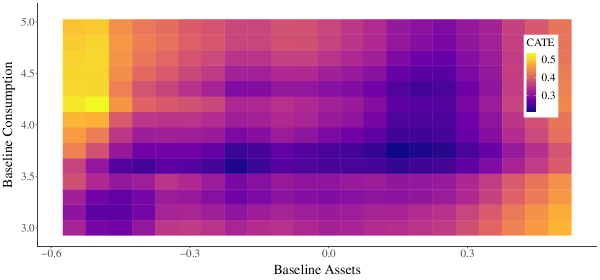 |
| Panel B: Lower Bound |
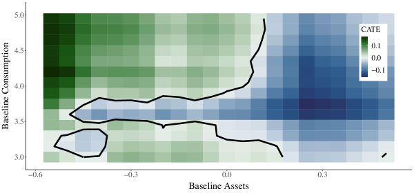 |
Notes: Figure D.1 displays heat maps giving binomial-sample upper and lower confidence bounds for the CATE of the intervention studied in Banerjee et al., (2015) on post-treatment total assets. The confidence bounds are constructed at level . The upper and lower bounds are displayed with different color palettes to emphasize the use of different scales. A contour line has been superimposed over the lower bound to demarcate where the bound crosses zero. The axes and estimator are the same as in Figure 1.
D.2.1. Proof of Theorem D.1, Part (i)
The result follows from an argument very similar to the proof of Theorem A.2, Part (ii). Again, we take for all , without loss of generality. Here, we are interested in studying the discrepancy
By analogy to (A.70), we can write
| (D.8) | ||||
| (D.9) |
where and are constructed with the subsample . Let denote the event that
| (D.10) |
Similarly, let and denote the events that
| (D.11) | ||||
| (D.12) |
respectively, where is again defined analogously to . Define the event . Fix a hyper-rectangle in , and again recall the normalized and enlarged hyper-rectangles and . On the event , we have
for each . Let be a random variable taking the value with is an element of the subset and taking the value otherwise. Observe that
| (D.13) |
and that the weights are independent and identically distributed Rademacher random variables. Thus, on the event , we have
| (D.14) |
with probability greater than by Lemmas A.1 and A.4. Hence, it suffice to give a high probability bound on for suitable choices of and .
To this end, observe that a multiplicative Chernoff bound implies that
| (D.15) |
with probability greater than . Thus, as the data are drawn independently and identically with distribution in and we have assumed that and for any fixed , by setting and , Assumption A.3 and the bound Equation A.51 imply that the event occurs with probability greater than , as required.
D.2.2. Proof of Theorem D.1, Part (ii)
Again, we take for all , without loss of generality. Recall from the proof of Theorem A.2, Part (iii), that is a random variable taking the value when is an element of the subset , and taking the value otherwise, and that
| (D.16) |
Define the object
We are interested in studying
where the notation denotes that the expectation is evaluated only over the random variables . On the event , defined in the proof of Theorem A.2, Part (iii), we have that
We can evaluate
as the weights are mutually independent.
Now, observe that
with probability greater than by Bernstein’s inequality. Thus, on the event , we find that
with probability greater than . By setting
and , Assumption A.3 and the bound (A.51) imply that the event occurs with probability greater than . Consequently, we find that
with probability greater than , as required. .
Appendix E Details Concerning Data and Simulations
In this appendix, we document our treatment of the Banerjee et al., (2015) data. Section E.1 details our acquisition and cleaning of these data. In Section E.2, we give further details concerning the construction of Figure 1 and Figure 2. Section E.3 discusses our simulation calibration.
E.1. Data
The data from Banerjee et al., (2015) were acquired from https://dataverse.harvard.edu/dataset.xhtml?persistentId=doi:10.7910/DVN/NHIXNT on September 10, 2021. The data from the graduation program implemented in Pakistan are considered in Chen and Ritzwoller, (2023) and Ritzwoller and Romano, (2023). Here, we consider the data from the graduation program implemented in Ghana, as it has a larger sample size.
The data record measurements of many pre-treatment and post-treatment outcomes for 2,606 individuals in the northern region of Ghana. Baseline survey measurements were made prior to the allocation of treatment. A multifaceted treatment, composed of productive assets, consumption support, health and nutritional education, and savings requirements was randomly allocated to 632 of the individuals. Banerjee et al., (2015) consider data from two endline surveys, made two years and three years after the initial asset transfer, respectively. For the purpose of this paper, we consider only data from the baseline survey, records of the treatment allocation, and measurements from the first endline survey. We omit data from 164 attrited individuals, none of whom were assigned to the treatment.
The covariate vector is composed of measurements of 16 pre-treatment outcomes. Five of these outcomes are associated with consumption: total monthly consumption and total monthly consumption on food, non-food, and durable commodities. Each consumption variable is measured in 2014 US dollars. We transform total monthly consumption to logs, base 10. Three of the variables are associated with assets, each of which is an index constructed from survey data measuring total assets, total productive assets, and total household assets. We transform the total assets measurement to logs, base 10. Five of the outcomes are associated with food security. These consist of four binary variables indicating different aspects of food security, e.g. did a child skip a meal, in addition to an index aggregating these measurements.202020There are individuals with missing values for the food security index. We impute these values with the median values of the food security index. The final four variables are associated with finance and income: the total amount of outstanding loans, the total amount of savings, income from agriculture, and total income from business. The covariate vector collects the total monthly consumption and assets for each individual. The outcome measures the total assets two years after the initial asset transfer. Again, we transform these measurements to logs, base 10.
E.2. Parameter Choices
E.3. Simulation Calibration
We calibrate a simulation to the Banerjee et al., (2015) data using a collection of Generalized Adversarial Networks (GAN) (Goodfellow et al.,, 2014). This approach to simulation design was proposed by Athey et al., (2021). Roughly speaking, a GAN is a pair of neural networks. The objective of the first network, the generator, is to generate data that looks like the Banerjee et al., (2015) data. The objective of the second network, the discriminator, is to discriminate between the real Banerjee et al., (2015) data and the data generated by the generator. These networks compete iteratively until convergence. The idea is that, after convergence, the generator is a good proxy for the true process that generated the Banerjee et al., (2015) data. We use the “WGAN” package associated with Athey et al., (2021).
To calibrate our simulation, we estimate three GANs. The first GAN estimates the distribution of the covariates , i.e., baseline consumption and baseline total assets. The second GAN estimates the distribution of conditional on . Recall that collects all baseline covariates, other than the covariates in . The third GAN estimates the distribution of conditioned on , , and . To generate an observation , we generate , generate conditioned on , and generate the potential outcomes and from the estimated distributions of conditioned on , , and and , respectively. The treatment indicator is is drawn i.i.d., Bernoulli with the observed probability in the Banerjee et al., (2015) data and we set . In this way, we know the true treatment effect for each unit in our simulation. We draw 10 million observations with this process. In the simulation, datasets of various sizes are sampled from this collection.
We use a related procedure to determine the true CATE at each value in the query-vector (i.e., the centers of each of the rectangles displayed in Figure 1). Specifically, for each in , we draw 100,000 observations from the distribution of conditioned on . We then draw observations and for each of these replicates, and compute the average of the true treatment effects . Figure E.2 displays these pseudo-true values of the CATE , alongside a reproduction of the estimates of the true CATE constructed with GRF. Our simulation design captures many of the same features of the data recovered by GRF, but gives a somewhat smoother picture of the CATE.
| Panel A: CATE Estimates |
 |
| Panel B: Calibrated CATE values |
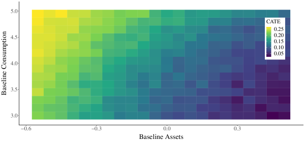 |
Notes: Figure E.2 displays heat-maps comparing GRF estimates of the CATE of the program considered in Banerjee et al., (2015) to the “true” value of CATE used in our calibrated simulation. Panel A recreates Figure 2. Panel B is constructed analogously.
Figure E.3 displays a scatterplot comparing the moments of the data from the Banerjee et al., (2015) data to the data generated by our calibrated simulation. The distributions match quite closely. Figure E.4 compares a scatter plot of the observed values of baseline consumption and baseline assets in the Banerjee et al., (2015) data with a heat-map of the distribution of these covariates in our simulation. The limits of the horizontal and vertical axes in this Figure match Figures 1 and 2 displayed in the main text. Some observations fall outside of the limits of this figure. The quartiles of baseline log consumption are 3.33, 3.76, and 4.20. The quartiles of baseline assets are -0.45, -0.71, and 0.03.
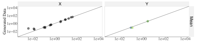 |
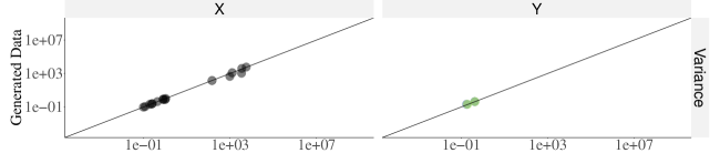 |
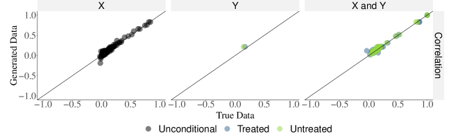 |
Notes: Figure E.3 displays scatterplots comparing the moments of the data from Banerjee et al., (2015) to the GAN generated simulation data. Columns differentiate between different types of variables. Rows differentiate between different types of moments. The x-axis of each sub-panel measures the moments of the true data. The y-axis of each sub-panel measures the moments of the generated data. The x and y axes in the first two rows are displayed in log-scale. A forty-five degree line is displayed in all sub-panels. Blue and green dots denote moments conditioned on treatment being set to one and zero, respectively. Black dots denote unconditioned moments.
| Panel A: Observed Covariates |
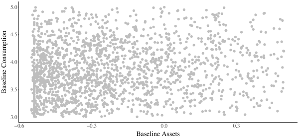 |
| Panel B: Simulation Covariate Density |
 |
Notes: Panel A of Figure E.4 displays a scatter plot of the observed values of baseline consumption and baseline assets in the Banerjee et al., (2015) data. The horizontal and vertical axes display the baseline monthly consumption, normalized to 2014 dollars on a logarithmic scale base 10, and an index for baseline assets, respectively. Panel B displays a heat-map giving the density of the joint distribution of baseline consumption and baseline assets associated with our calibrated simulation.