SceneFactory: A Workflow-centric and Unified Framework for Incremental Scene Modeling

Abstract

We present SceneFactory, a workflow-centric and unified framework for incremental scene modeling, that supports conveniently a wide range of applications, such as (unposed and/or uncalibrated) multi-view depth estimation, LiDAR completion, (dense) RGB-D/RGB-L/Mono//Depth-only reconstruction and SLAM. The workflow-centric design uses multiple blocks as the basis for building different production lines. The supported applications, i.e., productions avoid redundancy in their designs. Thus, the focus is on each block itself for independent expansion. To support all input combinations, our implementation consists of four building blocks in SceneFactory: (1) Mono-SLAM, (2) depth estimation, (3) flexion and (4) scene reconstruction. Furthermore, we propose an unposed & uncalibrated multi-view depth estimation model (U${}^{2}$-MVD) to estimate dense geometry. U${}^{2}$-MVD exploits dense bundle adjustment for solving for poses, intrinsics, and inverse depth. Then a semantic-awared ScaleCov step is introduced to complete the multi-view depth. Relying on U${}^{2}$-MVD, SceneFactory both supports user-friendly 3D creation (with just images) and bridges the applications of Dense RGB-D and Dense Mono. For high quality surface and color reconstruction, we propose due-purpose Multi-resolutional Neural Points (DM-NPs) for the first surface accessible Surface Color Field design, where we introduce Improved Point Rasterization (IPR) for point cloud based surface query. We implement and experiment with SceneFactory to demonstrate its broad practicability and high flexibility. Its quality also competes or exceeds the tightly-coupled state of the art approaches in all tasks. We contribute the code to the community.

I Introduction

Simultaneous Localization and Mapping (SLAM) plays an important role in robotics. Previous works have made substantial progress for robust localization of robots [1, 2, 3], including in challenging environments [4], while the mapping of the environment is often sparse. With the aim of producing higher quality maps, dense mapping [5] and 3D reconstruction [6] have been developed. Dense mapping provides a point set as a mapping representation, but is much denser. Alternatively, 3D reconstruction [6] produces meshes for compactness and continuity reasons, which is more user friendly.

However, we observe that most works construct the whole pipeline in a high tight-compact design. This restricts the model to a specific application and is difficult to upgrade each submodule. So this initiates our first research question: Can we design a framework that will support all of the production lines?

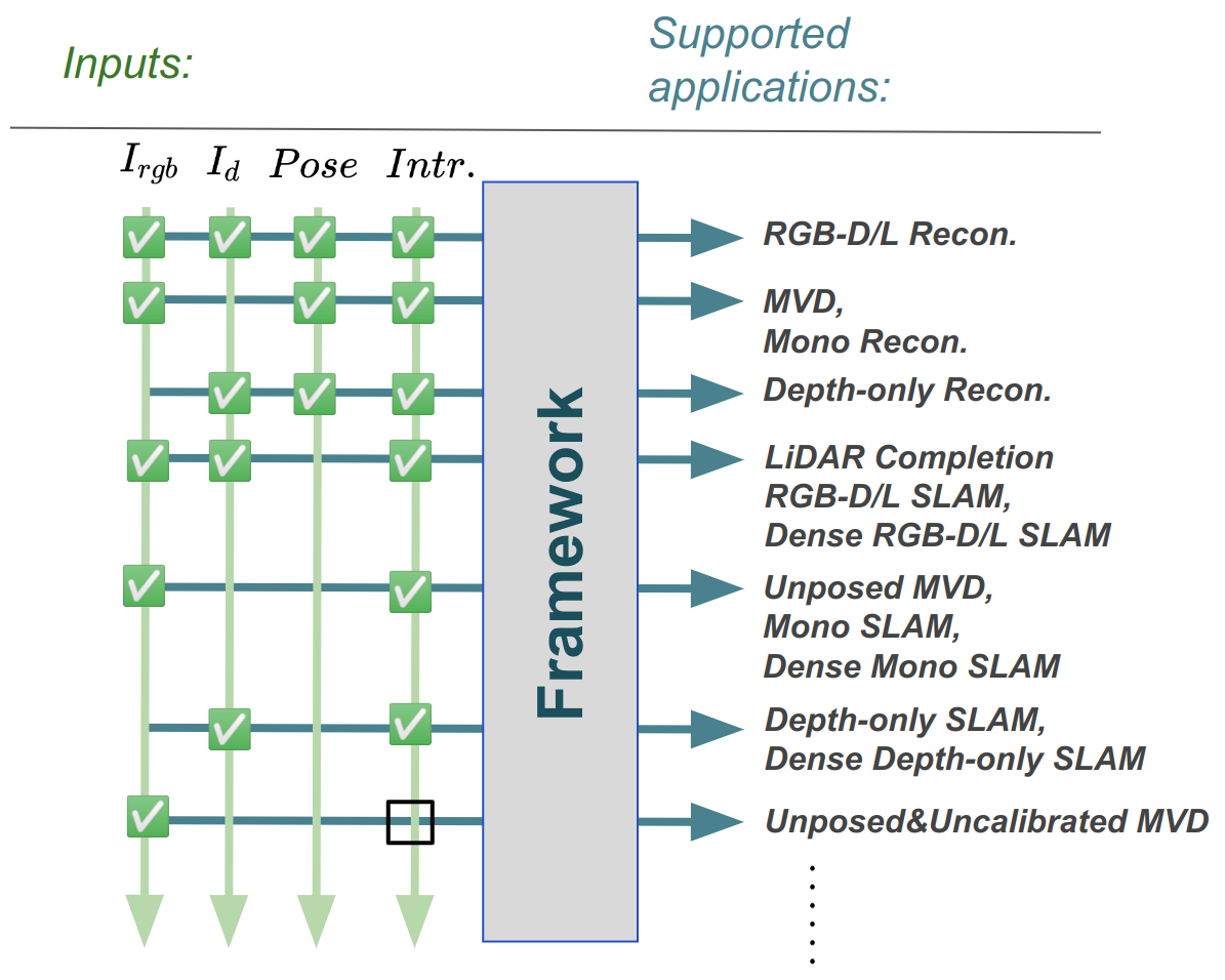
Figure 1: SceneFactory is workflow-centric and supports a wide range of applications given different input combinations of RGB $\mathbf{I}_{\text{rgb}}$, depth $\mathbf{I}_{\text{d}}$, pose $\mathbf{G}$ and intrinsics $\mathbf{\theta}$.

First of all, we do a traversal of all possible input cases and have a look at what the tasks might be. As shown in Fig. 1, given different input combinations of RGB $\mathbf{I}_{\text{rgb}}$, depth $\mathbf{I}_{\text{d}}$, pose $\mathbf{G}$ and intrinsics $\mathbf{\theta}$, a number of applications could be run. And our goal at the very beginning is to support them all in our single framework.

To achieve this goal, we design our framework in a workflow-centric way. The advantage of such a design philosophy is that all tasks are connected by a dependency graph to reduce redundancy. For example, as in our design Fig. 2, the final task usually depends on the other tasks. However, the other tasks can also be the final task. All subtasks work both independently and together, each block must be complete on its own. Thus, this brings us to four blocks in the workflow: tracker, density estimator, chromaticity estimator and reconstructor.

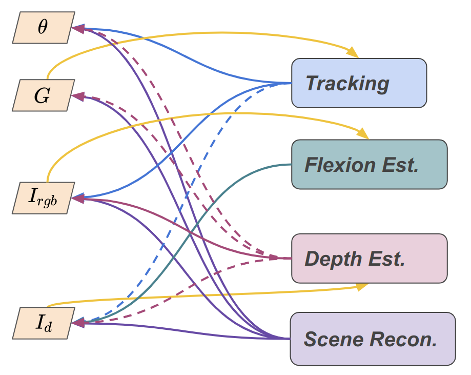
Figure 2: Dependency graph for SceneFactory. The solid line indicate strict dependency, while dash line indicate optional dependency. The links between application and blocks follows Fig. 1 and are not drawn. When pose $\mathbf{G}$/RGB $\mathbf{I}_{\text{rgb}}$/depth $\mathbf{I}_{\text{d}}$ is given, their dependency is filled without additional calling.

On the tracking block, we subtract and find the greatest common divisor, Mono-SLAM. Mono-SLAM considers more complicated conditions than RGB-D and Stereo SLAM because of the difficult depth estimation. Which operates the simplest sensor setup with less observation demands. However, Mono-SLAM relies on only sparse keypoints, and thus we further introduce a dense estimation task for dense depth-related applications. The “loose connection” concept directs us to build a dense SLAM where each module focuses on its own task.

This is followed by dense estimation, which is widely studied under the topic of dense monocular SLAM. Dense monocular SLAM is one of the most challenging branches of SLAM algorithms. To estimate the dense information, researchers currently rely on encoder-decoder to generate and then optimise the mono-depth code [7, 8], use deep multi-view stereo (MVS) for direct depth estimation [9], or estimate using optical flow to provide the dense correlation between keyframes [10, 11]. However, mono-depth naturally loses scale and intrinsic information, usually resulting in distorted structures. For MVS nets, they are overfitted with the trained camera intrinsic. They will be dysfunctional for custom cameras and new scenes. Therefore, we turn to optical flow for correlation search and use dense bundle fitting to estimate the dense structure. Our dense estimation design is also influenced by the observation that DROID-SLAM [10] and Sigma-Fusion [11] show much depth with a cone-like distortion. Focusing on the cone distortion, we make an analysis and provide a different solution than Rosinol et al. [11]. We find that the problems come from the non-covisible regions, the low texture regions and the in-plane epipole. For the first two, we find it is not the problem of the optical flow, because the optical flow is designed for tracking points, which does not assume a static environment. But for static, i.e., rigid scenes, this is detrimental for both pose and density estimation. Therefore, our first innovation is to add a static check to the optical flow based dense estimation. Second, for the in-plane epipole, since it cannot be shielded by static check, we simply precompute possible epipoles and remove related matches. However, the side effect of the above improvements will be missing regions in the depth image.

For use in SLAM sequences, we further introduce good neighborhood selection aiming to reduce the above situations. But even with this selection, the side effect of producing missing regions still exists. An example is in Section IV, where there is a hole in the wall. Inspired by MonoSDF [12], that the monocular depth shares point properties with the real depth, we turn to monodepth and find in our scene case that although monodepth is distorted between structures, in-structure coplanarity is preserved. Therefore, we propose to utilize this in-structure property with ScaleCov model. That relies on learned deep covariance to fill the clipped locations with regressed scale image. In SLAM related application, we additionally scale the depth to global to make the mapping consistent.

Even though our depth estimation model fits well into the Mono-SLAM, the model on its own supports unposed & uncalibrated multi-view depth estimation. Which further provides a user-friendly application that only RGB images are required.

Afterwards, for immersive visualization in 3D reconstruction, there have been some successful attempts recently, such as ESLAM [13] and NeRF-SLAM [14]. They borrow the NeRF-like training scheme to produce high quality view synthesis. However, the ray integration naturally suffers from many samples with large space and time cost. Therefore, we turn to another related branch, Neural Surface Light Fields (NSLF), without the optimization of geometry. Recent research of NSLF has verified the efficiency on SLAM sequences [15]. Because NSLF only learns surface field, each surface position is not modified. But, the existing online SLF method [15] requires an external SDF model [16] to provide the surface points. Therefore, we propose here due-purpose multi-resolutional neural points (DM-NPs) to overcome this limitation. Following NSLF-OL [15], which use a multi-resolutional hashgrid for efficient online learning, we create a multi-resolutional point grid for fast SLF learning. Moreover, since our point-based representation naturally provides position on surfaces, a straightforward idea is to use point rasterization. However, point rasterization is a dysfunction compared to surface rasterization (as introduced in Section III-C). To make it work, we propose Improved Point Rasterization to make it really useful compared to Pytorch3D[17]’s point rasterization. What’s more, our CUDA implementation is also 10 to 50 times faster than Pytorch3D’s CUDA implementation.

In summary, as shown in Fig. 1, we intend to design a modular scene modeling methods that each module supports individual applications, while it can be combined into ones.

The contributions of this work are:

1. We propose a workflow-centric framework, SceneFactory, that supports all incremental scene modeling applications with different combination under the connection of a dependency graph.

2. We propose a dual-purpose multiresolution neural points representation for both Surface Light Fields (SLF) and Improved Point Rasterization (IPR). Which is (1) the first surface-gettable SLF model, (2) the first to make point rasterization as usable as surface rasterization.

3. Propose a robust depth estimation block with (1) an unposed & uncalibrated multiview depth estimation model (U${}^{2}$-MVD) and (2) a deep correlation kernel based depth completion model, ScaleCov.

4. We capture the first dense mono-SLAM purpose RGB-X dataset for high quality monocular reconstruction.

In the following, we first describe the related work on dense monocular SLAM, neural rendering in SLAM and multi-view depth estimation. Then, in three separate sections, we introduce the due-purpose multiresolutional neural points representation, the unposed & uncalibrated depth estimation, and the whole SceneFactory structure. Afterwards, we conduct experiments to thoroughly evaluate the performance of the system. Finally, we conclude this paper and attach the supplementary.

II Related Works

II-A Dense SLAM

Textureless walls impose sensing challenges, since they can hardly be mapped in a mono or multi-camera setup. Thus, dense SLAM systems operate the dense depth from laser scanners or RGB-D sensors to approach a high quality surface reconstruction. When depth is involved, traditional fusion methods [18] incrementally update the Truncated Signed Distance Field (TSDF) and then extract afterwards a mesh using Marching Cubes [19]. More recently, neural priors are used for Neural Implicit Representation [16, 20].

Uni-Fusion’s implicit representation supports even more data properties without any training [21]. With the even more recent trend of volumetric rendering, trained neural implicit rendering methods also come into view [22, 15].

However, the application scenario of scanners and depth sensors is still limited by their low affordability, portability and accessibility. Alternatively, almost everyone has their own monocular camera at hand, e.g. in a mobile phone. Therefore, there are still some works in this direction in the last years.

Optimizing an entire sequence of depths is not feasible given the large number of variables involved. To reduce the computational costs of depth estimation, CodeSLAM [7] and DeepFactors [8] optimize the latent codes of depth images. However, the single-frame depth encoder-decoder needs to be pre-trained with similar data sets. Instead of optimizing poses and depths at the same time, Tandem [9] first solves frame poses and then uses pre-trained MVSNet to recover the dense structure. On the other hand, DROID-SLAM [10] ensembles dense optical flow modules into the pipeline, and optimizes poses and downsampled inverse depths using dense bundle adjustment. To cope with DROID-SLAM’s noisy depth estimation, Sigma-Fusion [11] introduces depth uncertainty into DROID-SLAM’s framework and uses TSDF to provide a high quality dense reconstruction.

Starting in 2022, more researchers realized the high potential of using NeRF for high quality mapping. Orbeez-SLAM [23] and NeRF-SLAM [24] first embedded NeRF in SOTA-SLAM frameworks. For example, Orbeez-SLAM generates a sparse map using OrbSLAM3 [25] to set up a coarse occupancy grid for on-ray point sampling. NeRF is then applied directly given the tracked poses. Orbeez-SLAM gets the high quality rendering from NeRF. But we find that it also inherits the problem of NeRF, especially for SLAM sequences. That it can hardly work with non-around-object sequences. While based on Sigma-Fusion, which provides dense depth in nature, NeRF-SLAM addresses the above problem by monitoring depth along with color.

II-B Neural Rendering in SLAM

In our view, neural rendering is a topic that has the potential to replace reconstruction for high quality mapping.

Major group of 3D reconstruction mainly relies on marching cubes to extract mesh from explicit [18] or implicit [16, 20, 21]. This is not an efficient update due to the complicated (implicit)-to-explicit-to-mesh steps. While the alternative view synthesis relies on rendering, shows a more direct way to extract visualization from implicit. View generation could be super efficient.

The success of neural rendering in SLAM begins with the invention of iMAP [26] and NICE-SLAM [22]. iMAP applies volumetric rendering to MLPs and optimizes poses and MLPs with photometric loss. NICE-SLAM, which improves the rendering base, replaces the MLPs with hierarchical feature grids. This further improves the surface quality. To avoid the problem we mentioned in Orbeez-SLAM, NICE-SLAM uses RGB-D sequences to provide depth information to avoid the convergence problem. NICE-SLAM certainly provides a good basis for neural rendering. However, it still has the problems that 1. it is not real-time capable, 2. the color result is of low quality.

To cope with this, Orbeez-SLAM and NeRF-SLAM give a solution by coupling SOTA-SLAM with SOTA-NeRF, instant-ngp [27]. On the other hand, NSLF-OL [15] focuses only on surface color, and produces real-time neural surface light field model to work together with an external real-time reconstruction model.

However, working alongside make SLF’s performance highly depends on the hosting reconstruction model. Therefore, in this work, we also propose to make SLF model supports surface extraction.

II-C Multi-view Depth Estimation

Depth from multi-view could be obtained from multiple ways, such as depth-from-video, multi-view stereo and pointmaps.

Depth-from-video directly estimates depth images and camera poses from video sequences with known camera intrinsics. DeMoN [28] firstly utilize deep learning technique to estimate the depth and motion with a single network. Not only operating on pair of images, DeepTAM [29] and DeepV2D [30] process more images with alternating mapping and tracking modules. However, according to [31], such methods are overfitted to the trained scale and camera parameters. Which are difficult to generalize to arbitrary real-world applications.

Multi-view stereo estimates 3D geometry from unconstrained images with given intrinsic and extrinsic information. Here we only focus on the depth image estimation from MVS. MVS is starting to get a boost with the trend of deep learning. DeepMVS [32], as the first deep network based method, aggregates sampled patchwise deep features to estimate full image depth. It has demonstrated the high potential of high quality depth estimation with deep learning. Similarly, MVSNet [33] learns a feature map for whole images and fuses multi-view information into one feature map. Then MVSNet’s design serves as mainstream for following deep learning models [34, 35, 36, 37].

Pointmaps methods start attracting more attentions from 2024. It uses dense 2D field of 3D points as geometric representation. Pointmaps are first used in visual localization [38, 39] and monocular 3D reconstruction [40, 41]. A recent pointmaps-based work DUSt3R [42], designs a flexible stereo 3D reconstruction model. DUSt3R groundbreakingly unifies different 3D tasks. For the first time, it also provides a user-friendly interface that does not require camera parameters.

Our work is partly inspired by the seminal work DUSt3R. On the one hand, we want to provide a user-friendly interface like DUSt3R. On the other hand, we want to provide a unified model for all possible 3D related scene modeling.

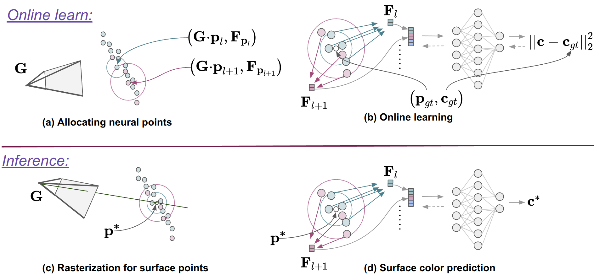
Figure 3: Illustration of the multiresolution neural points in 2D.

III Dual-purposes Multiresolutional Neural Points

In this section, we introduce the dual-purpose representation that simultaneously supports Surface Light Fields (SLF) and point rasterization. This representation is the first SLF method to support surface querying.

III-A Multiresolutional Neural Points

Intuitively, a neural point is a point with a feature. We denote a neural point as $\mathbf{v}=(\mathbf{F}_{v},\mathbf{p}_{v})$ with feature $\mathbf{F}_{v}\in\mathbb{R}^{m}$ and position $\mathbf{p}_{v}\in\mathbb{R}^{3}$.

Then, inspired by instant-ngp [27], we use multiresolution neural points to improve learning efficiency. These are multiple sets of neural points with different density. We denote them as $\mathbf{V}_{a}$ the set of $\mathbf{v}$ with resolution/density $a$.

During training, we follow NSLF-OL [15] to feed the set of colored pairs ${(\mathbf{p}_{i},\mathbf{c}_{i})}_{i}$ for coding and training. For each point position, we examine the density in its region and assign neural points. Then the MLP coding is applied.

III-A1 Neural Points Allocation

For the feedpoint set $\mathbf{Q}=\{\mathbf{p}_{i}\}_{i}$, given a set of resolutions $\mathbf{a}$, we downsample to get $\{\mathbf{Q}_{a}\}_{a\in\mathbf{a}}$. Then, for each point $\mathbf{p}_{i}$ in $\mathbf{Q}_{a}$, we check the closest distance to $a$ level neural points, if dist is greater than threshold $t_{a}$, the set of neural points is extended by adding this point and assigning it initialize with feature.

III-A2 Surface Points Encoding

SLF’s inference is on the surface, so this coding is an interpolation of the feature.

We draw a 2D illustration in Fig. 3. For inference point $\mathbf{p}\in\mathbf{Q}$, we utilize efficient KDTree to find its $K$ nearest neighbor ($\{\mathbf{v}^{a}_{k}\}_{k\in\{1,\cdots,K\}}$ with distance $\{d^{a}_{k}\}_{k\in\{1,\cdots,K\}}$) of inference point from each level.

The $a$ level feature is

$$F^{a}_{\mathbf{p}}=\sum_{i\in\{1,\cdots,K\}}w_{i}F^{a}_{v_{i}}$$ (1)

where $w_{i}=exp(-\frac{{d_{i}}^{2}}{\sigma})/\sum_{j}exp(-\frac{{d_{j}}^{2}}{\sigma})$.

III-A3 Color Prediction

Then the color prediction is generated by concatenating features along different levels and decoded with MLP: $f_{\text{MLP}}\circ f_{\text{concat}}((F^{a}_{\mathbf{p}})_{a\in\mathbf{a}})$.

III-B Mapping via Online Learning

We learn this SLF in an online fashion by continuously feeding data according to [15]. A main thread of this module is to continuously train the SLF. As soon as a new posed image with depth is input to the renderer, it is assigned a trained iteration, $it_{\text{trained}}$, to train in a least-touched strategy.

During the training iteration of a given frame, it randomly samples $n_{\text{train}}$ pixels and pass the corresponding point pairs $\{(\mathbf{p}_{n},\mathbf{c}_{n})_{n\in\{1,\cdots,n_{\text{train}}\}}\}$ to the neural allocation Section III-A1 and prediction Section III-A3 for the resulting color $(\mathbf{c}^{*}_{n})_{n}$.

We compute the MSE

$$L_{\text{MSE}}=\sum_{n\in\{1,\cdots,n_{\text{train}}\}}\parallel\mathbf{c}^{*}_{n}-\mathbf{c}_{n}\parallel^{2}$$ (2)

and use the Adam optimizer for stochastic gradient descent optimization of the features of neural points and MLP.

In addition, we use the following two strategy to speed up the training.

III-B1 Jump-start Training Strategy

From the experiment, we find that our SLF converges slowly on the first frame. While super fast for the following frames if the first frame gets rough color. Otherwise, the other frames would also be relatively slow.

We think the problem is from the chaos of parameters as it is randomly initialized. So we set a $10\times$ higher learning rate for the first $5$ iterations and recover then. This way, even the first image converges in a second.

III-B2 Least-trained First Training Strategy

The second training strategy is that after the first frame, when another frame is input, the previous well-trained frame shouldn’t have the same chance to be trained as the new one. So an intuitive way is to always train the least trained frame.

In this way, all subsequent frames are converged in one second.

III-C Improved Point Rasterization (IPR)

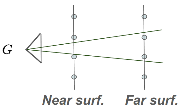
Figure 4: Near-far-imbalance.

Above is the training process where the depth is given. During the inference, we have to estimate the depth. Therefore, point rasterization is introduced.

For simplicity, we will now operate on points in camera space. To render an image with a resolution of $H\times W$, we cast a batch of rays $(\mathbf{o}_{i}=\mathbf{0},\mathbf{d}_{i}\in{\mathbb{S}^{2}})_{i\in\{1,\cdots,HW\}}$ with $(\mathbf{o},\mathbf{d})$ as the ray source and direction.

On the other hand, the positions of the neural points are first transformed into NDC space.

Set camera space point $\mathbf{p}=[X,Y,Z]^{T}$ as an example, projected point in NDC is then $\mathbf{p}_{\text{ndc}}=[f_{x}\frac{X}{Z}+p_{x},f_{y}\frac{Y}{Z}+p_{y},\frac{1}{Z}]^{T}$. Where $(f_{x},f_{y},p_{x},p_{y})$ are intrinsic parameters. In this way, each ray is directed to $+z_{\text{ndc}}$, i.e., $\mathbf{d}_{\text{ndc}}=[0,0,1]^{T}$. The source of the NDC space ray is obtained by projecting $\mathbf{d}$ accordingly.

Points within a radius $r_{\text{ndc}}$ around each ray $(\mathbf{o}_{\text{ndc}}=[x_{\text{ndc}},y_{\text{ndc}},z_{\text{ndc}}]^{T},\mathbf{d}_{\text{ndc}})$ are then computed using only the $(x,y)$ coordinate.

Thus, for each ray $(\mathbf{o},\mathbf{d})_{i}$, we find its $K_{\text{ray}}$ nearest neural point neighbors and the distance $\{(\mathbf{p}_{nb,k},d_{nb,k})\}_{k\in\{1,\cdots,K_{\text{ray}}\}}$ within the radius. The rasterized point is thus

$$\mathbf{p}_{\text{raster}}=\sum_{k\in\{1,\cdots,K\}}w_{nb,k}\mathbf{p}_{nb,k}$$ (3)

where $w_{nb,k}=exp(-\frac{{d_{k}}^{2}}{\sigma})/\sum_{j}exp(-\frac{{d_{j}}^{2}}{\sigma})$. However, unlike mesh rasterization, point rasterization suffers from the following problems:

1. the point distribution in NDC space is distorted. That is, the points near the camera are more sparse while the points far from the camera are more dense compared to Euclidean space. This results in holes in the near region.

2. the rasterization may contain several layers of points.

To deal with 1) the hole problem, we introduce an adaptive radius to PR. This changes the radius depending on the depth.

Considering that our finest resolution is $r=0.005m$ and the screen space is at $z=1$, we expect that each point with a $0.005m$ gap can completely cover a pixel at $z=1$. The coverage radius should be $l_{\text{coverage}}=\sqrt{2}(r\cdot f_{im})$ where $f_{i}m$ is the focal length parameter. To simplify the implementation, our CUDA code creates a $l_{\text{coverage}}\times l_{\text{coverage}}$ window for this point.

If $z<1$, the scenario in Fig. 4 can occur because the points are distorted in the screen space. The ray will then penetrate the near surface. To solve this problem, we increase the coverage area, the coverage length becomes $l_{\text{coverage}}=\sqrt{2}(r\cdot f_{im})/z$.

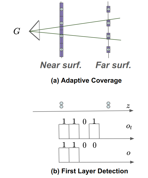
Figure 5: Improved Point Rasterization.

For the 2) problem of multiple layers, we propose to use first-layer detection to keep only the points of the first layer. Given $n$ and $z$-axis ascending sorted points traced by a given ray, $\{\mathbf{z}_{0},\cdots z_{n}\}$, we compute the occupancy of point $z_{t}$.

$$o_{t}=\left\{\begin{aligned} 1\ \ \ \ \ \ \ \ &&&t=0,\\ z_{t+1}-z_{t}<th&&&t>0.\\ \end{aligned}\right.$$ (4)

Then, by cumulating production, we get the mask of the first layer points:

$$o_{\{0,\cdots\}}=cumprod(o_{\{0,\cdots\}}).$$ (5)

We implement our IPR with CUDA, which is about 20 times faster than Pytorch3d’s CUDA implementation (40 FPS vs 2 FPS). We demonstrate the effect of IPR in Suppl.-B.

III-D Visualization

This function plays an important role in rasterizing the depth image and extracting the surface point colors under certain viewpoints. First, we rasterize at the level of neural points with the highest resolution. Then, transforming back to world coordinates with $\mathbf{T}$, the color prediction is obtained by

$$\mathbf{c}_{raster}=f_{MLP}\circ f_{concat}((F^{a}_{\mathbf{T}\mathbf{p}_{raster}})_{a\in\mathbf{a}}).$$ (6)

We follow [15] to create another thread with an interactive GUI to provide a first-person view of the scene.

This thread gets a signal from the user to rotate and move the view camera. The view synthesis is rendered in real time.

IV Depth Estimation

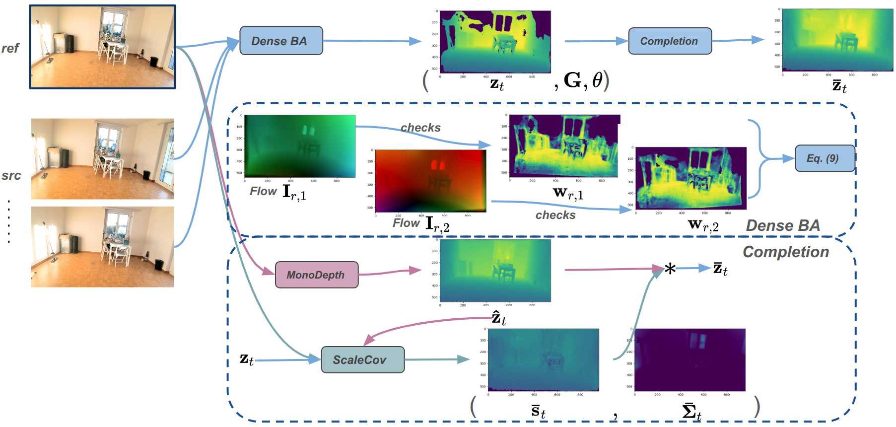
Figure 6: Depth estimation via unposed & uncalibrated multi-view depth estimation model (U${}^{2}$-MVD).

In this section, we introduce our unposed & uncalibrated multi-view depth estimation model (U${}^{2}$-MVD) that is depicted as in Fig. 6. As an adjunct to SLAM, we additionally add good neighbor frame selection for more suitable frames.

IV-A Depth Recovery with Dense Correlation

We acquire dense correspondences from SOTA optical flow estimation model DKMv3 [43] for pixel-wise correspondences $\mathbf{l}_{i,j}\in\mathbb{R}^{H\times W\times 2}$ between the frames $i$ and $j$. Then the expected correspondence pixel would be $\mathbf{x}_{j}^{*}=\mathbf{l}_{i,j}+\mathbf{x}_{i}$, where $\mathbf{x}_{i}$ is the pixel coordinate in frame $i$. However, if false correspondences occur, it will strongly affect the resulting pose and depth. That is, the optical flow cannot be fully trusted.

IV-A1 Cross Check

Because single-source matching is risky, we apply cross-checking of correspondences to ensure a high quality match:

$$\mathbf{w}_{i,j,(u,v)}=\begin{cases}1&\text{if }||\mathbf{x}_{i,(u,v)}-(\mathbf{x}^{*}_{j,(u,v)}+\mathbf{I}_{j,i,(u,v)})||_{2}<0.5,\\ 0,&\text{otherwise}\end{cases}$$ (7)

where $(u,v)$ is the pixel coordinate in the image.

IV-A2 Static Check

We have assumed that our scene is static. However, optical flow is not designed for static scenes. That is, the flow is not constrained by the rigid body. Therefore, unlike previous works [10] that trust the flow, we apply epipolar constraint to filter out the non-rigid flow:

$$\mathbf{w}_{i,j,(u,v)}=\begin{cases}1&\text{if }dist_{line}(\mathbf{L}_{j,(u,v)},\mathbf{x}^{*}_{j,(u,v)})^{2}<3.84,\\ 0,&\text{otherwise}\end{cases}$$ (8)

where $\mathbf{L}_{j,(u,v)}$ is the epipolar line for $\mathbf{x}^{*}_{j,(u,v)}$, $dist_{line}$ is the distance from point to line. The epipolar line $\mathbf{L}_{j}$ is obtained by solving the essential matrix with $1000$ randomly chosen correspondences.

IV-A3 In-image Epipole Check

However, since the above static check relies on the epipolar constraint, this check does not work near the epipole, i.e., if the epipole is in the image, the near pixels will all pass the static check.

Therefore, we compute the epipole position in image and filter out the near pixel correspondences.

IV-A4 Dense Bundle Adjustment (DBA)

Although the SOTA optical flow is used, from experiment, single flow is still too fragile for dense reconstruction use.

Therefore, more source frames are usually involved in MVD tasks. In our formulation, we project reference frame’s depth to all source frames and supervise via dense correspondences between each reference-source pair ($\mathcal{B}_{t}$). In connecting with SLAM, we also collect dense matching from reference (frame $t$) to neighbor frames ($\mathcal{B}_{t}$) in window, and compute dense BA to stabilize the inverse depth of reference frame $\mathbf{d}_{t}$.

Then we follow DROID [10, 44] to denote the poses, the intrinsics and the projection function as $\mathbf{G}$, $\mathbf{\theta}$ and $\Pi$. The cost function of the Dense Bundle Adjustment (DBA) would be the sum of the projection errors over all neighboring frames:

$$\mathcal{L}(\mathbf{G},\mathbf{d}_{t},\mathbf{\theta})=\sum_{j\in\mathcal{B}_{t}}\parallel\mathbf{x}^{*}_{j}-\Pi(\mathbf{G}_{tj}\circ\Pi^{-1}(\mathbf{x}_{t},\mathbf{d}_{t},\mathbf{\theta}),\mathbf{\theta})\parallel^{2}.$$ (9)

This cost function is solved efficiently with Gaussian-Newton. For the detailed formulation, please refer to DROID-SLAM [10, 44]. Eq. 9 directly solves poses, intrinsics and inverse depth at the same time with only optical flow (dense correspondences) as true value.

IV-A5 Monocular Depth and Depth Completion

In addition to the DBA, we utilize Metric3Dv2 [45] for monocular depth $\mathbf{\hat{z}_{t}}$ on the reference frame $t$. $\mathbf{\hat{z}_{t}}$ could help the DBA from a good start point. While more importantly, we use $\mathbf{\hat{z}_{t}}$ to assist completing the DBA depth with vacancy.

Recent monocular depth methods [46, 45] provide high quality depth estimation of structures. However, because the estimation from a single image naturally loses scale and intrinsic information, as in Fig. 7b, the relative positions between different structures are distorted. Besides, monodepth suffers vision illusion such as Ames room in Fig. 13. Which make inter-structure of monodepth theoretically not reliable.

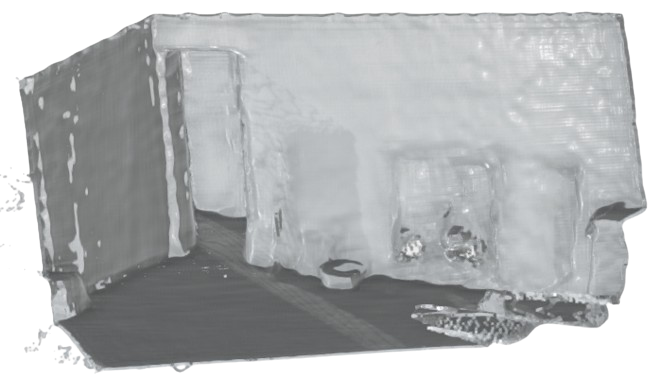
(a) width=.5

[width=.5][Over view]

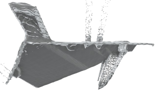
(b) Monocular depth example.

Nevertheless, we still find useful information: the coplanarity is preserved. Which reminds us to extract useful information from intra-structure.

Thus we intend to utilize learned covariance function that can semantically identify intra- and extra-structures. We find that DepthCov [47] learns deep prior. However, a problem of DepthCov is that it directly regresses depth image with true sparse depth observation. This means that if there is no true sample on certain structure, the depth of that structure would be arbitrary wrong. An extreme example is with only $1$ sample, then the whole depth image will be the same value.

Conversely, we introduce ScaleCov, which regresses scale image for monodepth $\mathbf{\hat{z}_{t}}$ given DBA depth $\mathbf{z_{t}}$ as observation. ScaleCov does not face this problem, because in the worst case identical scale image does not ruin the depth structures.

Following DepthCov, we utilize its deep learned covariance function (kernel function) $K$ to formulate ScaleCov as

$$\mathbf{s}_{*}=\mathbf{K}_{fn}(\mathbf{K}_{nn}+\sigma_{n}^{2}\mathbf{I})^{-1}\mathbf{s}_{n},$$ (10)

$$\mathbf{\Sigma}_{*}=\mathbf{K}_{ff}-\mathbf{K}_{fn}(\mathbf{K}_{nn}+\sigma_{n}^{2}\mathbf{I})^{-1}\mathbf{K}_{nf}.$$ (11)

Where, we sample non-vacancy depth from DBA depth and compute scales $\mathbf{s}_{n}=\mathbf{z}_{t,n}/\mathbf{\hat{z}}_{t,n}$, and use $\mathbf{K}_{ff}$, $\mathbf{K}_{fn}$ and $\mathbf{K}_{nn}$ to denotes the correlation matrix between query points, query and observations, and observations. $\mathbf{s}_{*}$ and $\mathbf{\Sigma}_{*}$ are the queried scale and variance that would be associated with the depth image.

For the finished image we consider the depth to be complete is more trustworthy and let

$$\mathbf{\bar{s}}_{t}(\mathbf{x})=\begin{cases}\mathbf{z}_{t}(\mathbf{x})/\mathbf{\hat{z}}_{t}(\mathbf{x}),&\text{if }\mathbf{z}_{t}(\mathbf{x})>0\\ \mathbf{s}_{*}(\mathbf{x}),&\text{otherwise}\end{cases}$$ (12)

$$\mathbf{\bar{\Sigma}}_{t}(\mathbf{x})=\begin{cases}\mathbf{0},&\text{if }\mathbf{z}_{t}(\mathbf{x})>0\\ \mathbf{\Sigma}_{*}(\mathbf{x}),&\text{otherwise}\end{cases}$$ (13)

where $\mathbf{x}$ the pixel coordinate.

The final completed depth is

$$\mathbf{\bar{z}}_{t}=\mathbf{\bar{s}}_{t}*\mathbf{\hat{z}}_{t}$$ (14)

where the corresponding pixel-wise variance is $\mathbf{\bar{\Sigma}}_{t}$.

In addition to the MVD completion shown in Fig. 6, ScaleCov can also support sparse LiDAR depth completion as shown in Fig. 21b.

IV-B Depth Frame Selection

We observe that all previous dense mono SLAMs estimate global geometry using keyframes. It makes sense to estimate depth for keyframes because during the tracking process, the main burden of keyframes is to gain information. The goal is to keep the landmarks in view.

However, we find it problematic to use neighbor keyframes to support depth recovery. This does not guarantee a good basis for triangulation, especially in dense cases.

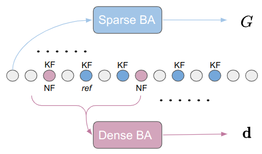
Figure 8: Pose and depth computation.

Therefore, as abstracted in Fig. 8, the good neighbor frames (NF) may not be keyframes (KF). In addition, the tracking model stores non-KF poses as a relative pose to the previous KF. This may not be accurate. While using our depth model, we only input intrinsics and images to estimate the depth without using the poses of the NFs.

Next, we ask the question: “How to choose a frame that is good for depth estimation?”

Reliable depth estimation requires a reference frame for triangulation. Therefore, our answer is: “A frame has a good neighborhood for triangulation”.

Because the tracking model provides poses for all frames, we can use the relative poses to the reference frame to help verify. We select neighboring frames according to Algorithm 2, where the relative facing angle and baseline are used.

IV-C Recover Scale to Global

Since Section IV-A is applied without poses, a scale recovery operation is required to adjust to the tracking scale.

While the global scale is hidden in the tracked landmarks or provided poses.

When landmarks are given, the relative scale from local to global is recovered by using RANSAC regression $s_{t,g}=RANSACRegressor(\{\mathbf{z}_{t}^{l}(\mathbf{x})/\mathbf{\bar{z}}_{t}(\mathbf{x})*s=1\}_{\mathbf{x}\in\mathcal{P}_{t}})$, where $\mathbf{z}_{t}^{l}$ and $\mathbf{\bar{z}}_{t}$ are the landmarks from the tracker and the estimated depth from Section IV-A, $\mathcal{P}_{t}$ and $\mathbf{x}$ are the set of landmarks in frame $t$ and pixel coordinate.

When landmarks are missing (use provided poses), we adjust depth with the scale difference between solved and provided poses.

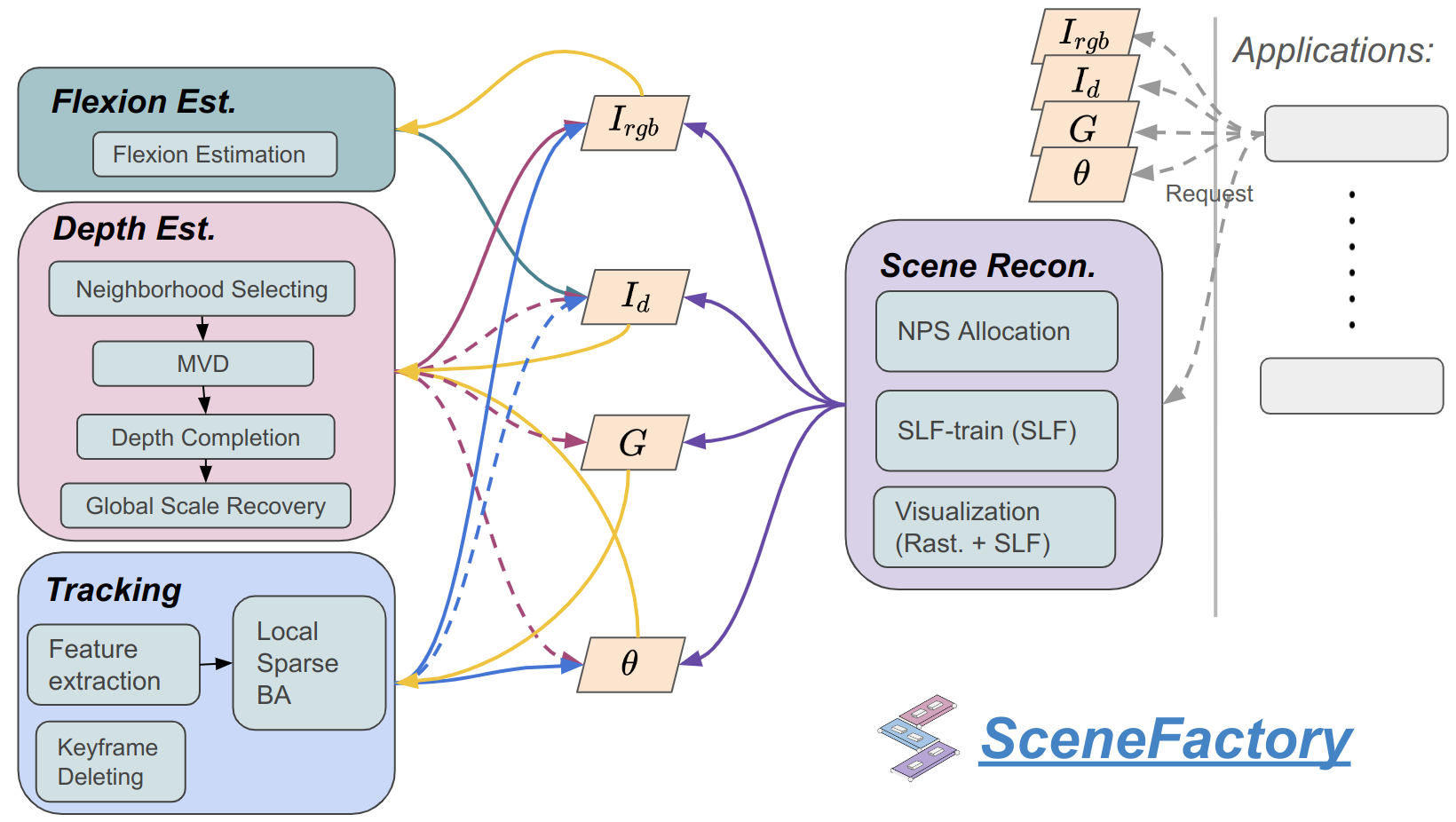
Figure 9: The dependency graph in SceneFactory. The yellow line indicates the dependency edge when the value is None. The green, purple, blue, and pink lines indicate the dependency edge of the Bending, Depth, Tracking, and Scene Reconstruction blocks. The gray line indicates the requirement of a specific application. The solid/dotted line shows mandatory/optional dependency. Inside of each module, the black arrow indicates the pipeline.

V A Unified Framework for Incremental Scene Modeling

SceneFactory supports various combinations of $\mathbf{I}_{rgb}$, $\mathbf{I}_{d}$, $\mathbf{G}$ and $\mathbf{\theta}$ as input. We plot the entire pipeline in Fig. 9 to have a brief overview. All of the applications in Fig. 1 can find their corresponding parts in this diagram.

SceneFactory consists of four building blocks:

• flexion estimation block to the complete the image,

• depth estimation block to estimate and complete the depth,

• tracking block to complete pose,

• scene reconstructing block.

In this section, we introduce each of these blocks respectively (Sections V-B, V-C, V-A and V-D) and combine them to a whole workflow (Section V-E).

V-A Tracking Block

For the tracking block, we use Mono-SLAM because it is a greatest common divisor with minimal demands. More specifically, our tracking block is based on DPVO [48], while we generalize it to also to support RGB-D/L input.

DPVO is based on sparse correspondences, while the pose $\mathbf{G}$ is optimized with sparse bundle adjustment:

$$\mathcal{L}_{track}(\mathbf{G},\mathbf{P})=\sum_{(k,j)\in\mathcal{E}}\parallel\Pi(\mathbf{G}_{ij}\circ\Pi^{-1}(\mathbf{P}^{{}^{\prime}}_{k}))-[\hat{\mathbf{P}}^{{}^{\prime}}_{kj}+\delta_{kj}]\parallel_{\Sigma_{kj}}^{2}.$$ (15)

where $\mathbf{P}^{{}^{\prime}}_{k}$ is the patch $k$ in image $i$, $\hat{\mathbf{P}}^{{}^{\prime}}_{kj}$ is the center of patch $\mathbf{P}^{{}^{\prime}}_{kj}$ in image $j$, $\delta_{kj}$ is the patch update.

The above formulation is solved efficiently with Gauss Newton. When the depth $\mathbf{I}_{d}$ is given, we extract patch $\mathbf{P}$ from the corresponding position. We fix the patch from valid depth pixel and optimize only the poses $\mathbf{G}$ from $\mathcal{L}_{track}$ with Gauss Newton. We choose DPVO for the generalization because it does not require explicit extraction of matches, and thus well fit the sparse observation of the LiDAR. From our experiment, this generalized version is more accurate by utilizing the metric depth.

V-B Flexion Estimation Block

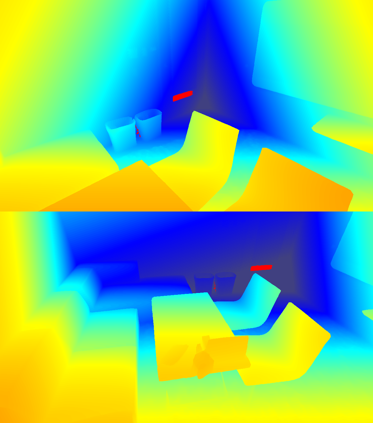
(a) Colorized depth

(b) Flexion

Figure 10: Depth images and their correspondingly converted flexion images.

Flexion estimation is required when $\mathbf{I}_{rgb}$ is missing (depth only).

To support depth-only tracking in our RGBD SLAM framework, a feature matching operation is required. However, the depth image does not contain the SE3-invariant context for descriptor extraction.

Therefore, we use the seminal depth converter [49] to convert the depth image into a flexion image that has the SE3-invariant properties. An example is given in Fig. 10b. We colorize the depth only for better visualization. We see that flexion images contain a more consistent value, which is more suitable for feature matching [49].

Therefore, depth-only applications are able to treat flexion as RGB and serve as RGBD applications as in Fig. 22.

V-C Depth Estimation Block

The depth estimation block is mainly our U${}^{2}$-MVD (in Section IV) with intrinsics given for pose-free MVD to support incremental application. It fills the depth void for RGB applications, allowing them to work as RGB-D applications.

Note that when no metric depth is specified, tracking frames only requires sparse-BA with images. Depth estimation is only required when KF and NFs are detected or MVD is called for certain application requests. Once requested, this block will query memory for good neighbor selection (Section IV-B), pose-free MVD (Section IV-A), depth completion (Section IV-A5) and scale recovery (Section IV-C).

We put the depth estimation behind the tracking sequences because the tracker’s sparse BA will also optimize poses in a local window, the updated landmarks will affect the scale recovery.

V-D Reconstruction Block

The reconstruction block uses our DM-NPs presented in Section III. This block maintains two threads: 1) NPs allocation and online learning, and 2) visualization.

V-D1 Online-learning thread

A training thread is used to continuously train our SLF model. As soon as a new keyframe with ($\mathbf{I}_{rgb}^{{}^{\prime}}$, $\mathbf{I}_{d}^{{}^{\prime}}$, $\mathbf{G}^{{}^{\prime}}$) is input to the renderer, it is assigned a trained iteration, $it_{trained}$, to train in a least-touch-first strategy.

During the training iteration of a given frame, it will randomly sample $n_{train}$ pixels and pass the corresponding point pairs $\{(\mathbf{p}_{n},\mathbf{c}_{n})_{n\in\{1,\cdots,n_{train}\}}\}$ to the neural allocation Section III-A1 and prediction Section III-A3 for the resulting color $(\mathbf{c}^{*}_{n})_{n}$.

We compute the MSE

$$\mathcal{L}_{MSE}=\sum_{n\in\{1,\cdots,n_{train}\}}\parallel\mathbf{c}^{*}_{n}-\mathbf{c}_{n}\parallel^{2}$$ (16)

and use the Adam optimizer for a stochastic gradient descent optimization of neural point features and MLP.

V-D2 Visualization thread

Another thread for the renderer is to provide an interactive GUI to provide a first person view of the scene.

This thread gets a signal from the user to rotate and move the view camera. The view synthesis is rendered in real time (Section III-D).

V-E Main Function

SceneFactory’s main functions are $EstablishProductLine$ and $Step$ as in Algorithm 1.

1 Function $EstablishProductLine$($(\mathbf{I}_{rgb}$, $\mathbf{I}_{d}$, $\mathbf{G}$, $\mathbf{\theta}$, $app)$):

       // Build product line

2       $pLine=AssemblingParts(\mathbf{I}_{rgb}$, $\mathbf{I}_{d}$, $\mathbf{G}$, $\mathbf{\theta}$, $app)$;

3       return $pLine$;

4

5End Function

6 Function $pLine.Step$($(\mathbf{I}_{rgb}$, $\mathbf{I}_{d}$, $\mathbf{G}$, $\mathbf{\theta}$, $app)$):

       // Product line start working part-by-part

7       $\mathbf{V}_{inter}\leftarrow pLine.Package(\mathbf{I}_{rgb}$, $\mathbf{I}_{d}$, $\mathbf{G}$, $\mathbf{\theta}$, $app)$;

8       for $f_{part}$ in pLine.parts do

9            $\mathbf{V}_{inter}=f_{part}(\mathbf{V}_{inter})$

10       end for

11      return $pLine.Unpackage(\mathbf{V}_{inter})$;

12

End Function

Algorithm 1 Main functions

When a task is triggered, SceneFactory successively checks the availability of image $\mathbf{I}_{rgb}$, pose $\mathbf{G}$, depth $\mathbf{I}_{d}$ and intrinsics $\mathbf{\theta}$, to prepare the product line ready. Then the operation are conducted following Fig. 9.

For example, if $\mathbf{I}_{rgb}$ is missing (depth only), flexion block (Section V-B) is added to the product line to estimate the trackable image from depth. If SceneFactory is required to solve intrinsics without a $\mathbf{\theta}$ input, it will add intrinsic-free DBA to the line for $\mathbf{\theta}$. If SceneFactory is asked to solve poses without poses $\mathbf{G}$ as input, it will add a tracker to the line for predicting the pose $\mathbf{G}^{{}^{\prime}}$. If the metric depth is missing, depth estimator block (Section V-C) will be added for estimating the depth. While if the metric depth input is sparse (from LiDAR), only the depth completion part will be added. When reconstruction is requested by the application, the completed frame parameters with image, depth, pose and intrinsics are required to be fed into the reconstruction block (Section V-D) for online learning and visualization. And corresponding parts are all be added to the product line.

Then the product line treats each step function as a task. If a single task is requested (such as MVD, Completion and etc.), production line will return the step result as a product. While if sequential application is requested (such as SLAM, Reconstruction and etc.), product line will conditionally step on each frame for the intermediate and return product at the end of this production process.

VI Experiments

The main experiments are conducted on multi-view depth estimation, surface light field and Dense SLAM.

VI-A Settings

VI-A1 Implementation Details

We use $l=3$ levels of neural points with resolution starting at $r_{0}=0.005m$ with multiplier $m_{reso}=4$. Our reconstruction model uses the Adam optimizer with $lr=1e-3$ for both NPS and MLP. The k-nearest neighbor search between query and NPS is done with KD-Tree, while the rasterization is done with our CUDA-implemented IPR. For the depth estimation model, we rely on DKMv3 [43] for dense correspondences (optical flow), and Metric3Dv2 [45] for monocular depth. We follow DepthCov [47] to build our ScaleCov for depth completion. We extend the monocular tracking model DPVO [48] to RGB-D and RGB-L. Due to the optimization of local windowed frames, we only allow out-of-window (fixed) frames for depth and reconstruction. All experiments are conducted on a PC with an Intel i9-13900KSi9-13900KS CPU and an NVIDIA GeForce 4090 GPU.

VI-A2 Datasets

Our experiments mainly rely on datasets for scenes:

Replica [26]

Replica has recently become the most widely used synthetic dataset for reconstruction and synthesis of views. It consists of 8 RGB-D sequences for rooms and offices.

ScanNet [50]

ScanNet is also widely used for RGB-D reconstruction. However, ScanNet is captured with old camera sensors with high motion blur. Which is harmful for dense matching.

KITTI [51]

The KITTI dataset is one of the most famous outdoor dataset with stereo camera, Velodyne laserscanner and GPS. We use its depth completion data branch for RobustMVD benchmarking.

ETH3D [52]

ETH3D is a widely used benchmark in the field of 3D reconstruction. This dataset provides multi-view images with ground truth poses and mesh reconstruction. We use its multi-view benchmark data branch for RobustMVD.

DTU [53]

DTU is the most widely used object-level dataset in deep learning based multi-view stereo work. DTU provides high quality images with dense point cloud for each object. Although the tabletop object is not the research focus of this paper, we use DTU for RobustMVD.

Tanks&Temples [54]

Tanks&Temples captures real indoor and outdoor scenes with high quality videos. It is mostly used alongside the DTU dataset for generalization testing. We also use it for RobustMVD.

Our Dataset

We acquire the first dense mono-SLAM purpose RGB-X dataset. Previous RGB-D reconstruction purpose dataset contains large rotations, which is acceptable for RGB-D SLAM even with blur. However, for dense monocular purpose, sufficient parallax between consecutive frames is required. Large rotations and blurry images are detrimental to both tracking and depth estimation. Moreover, recent SOTA Dense Mono-SLAM only focus on small room- or object-scale reconstruction. With our own datasets we also want to show that the proposed method scales to larger scenes. Therefore, we acquire our own dataset using a motion pattern with good parallax and four different sensor systems, which are depicted in Fig. 11 (More detail place find Suppl.-C). The datasets ordered from small to large scale are:

• Apartment living room using Xiaomi Phone (RGB)

• University of Würzburg Robotics hall using a Kinect Azure (RGB-D)

• Veitshöchheim Palace captured from a handheld mapping system (RGB-L)

• University of Wüzburg building complex captured from an UAV of the Center for Telematics (RGB-L)

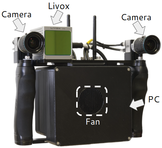
(a) width=0.45

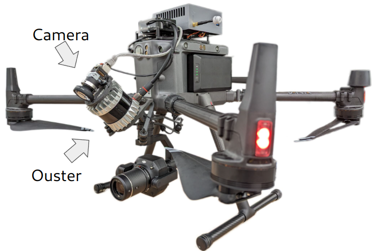
(b) width=0.5

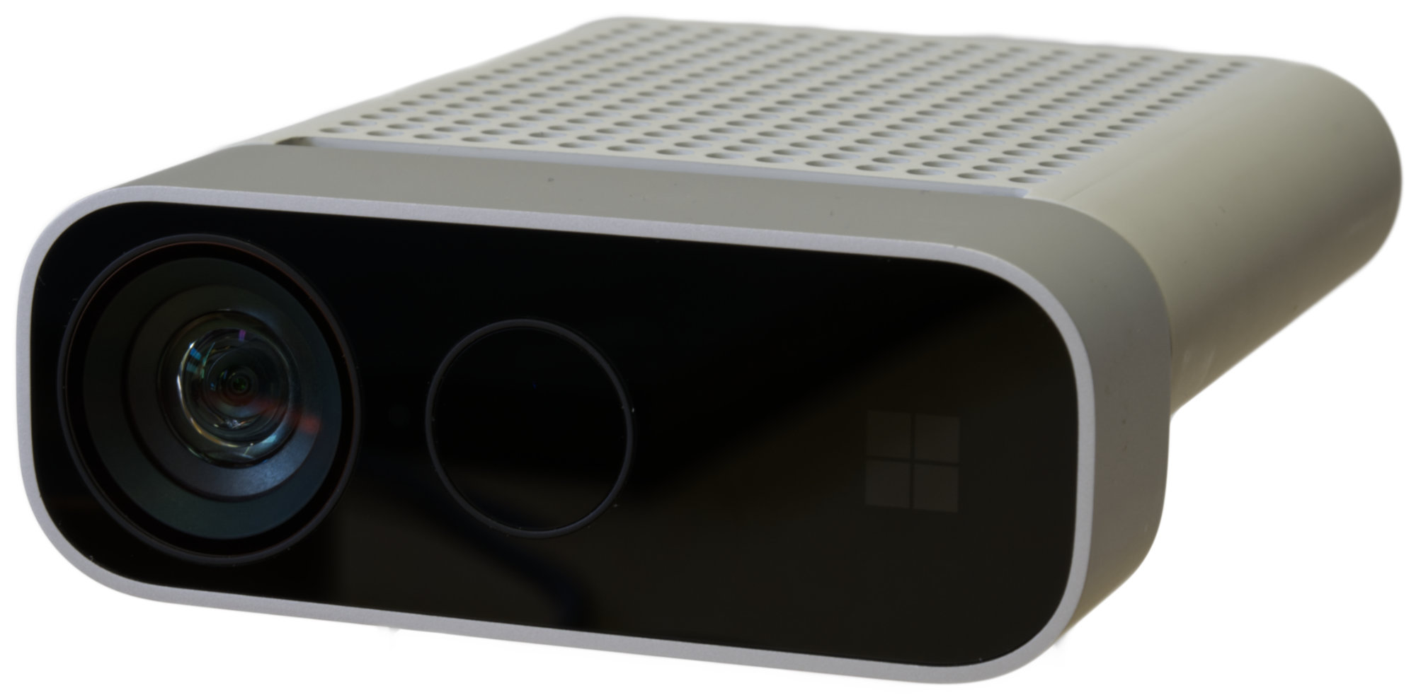
(c) width=0.4

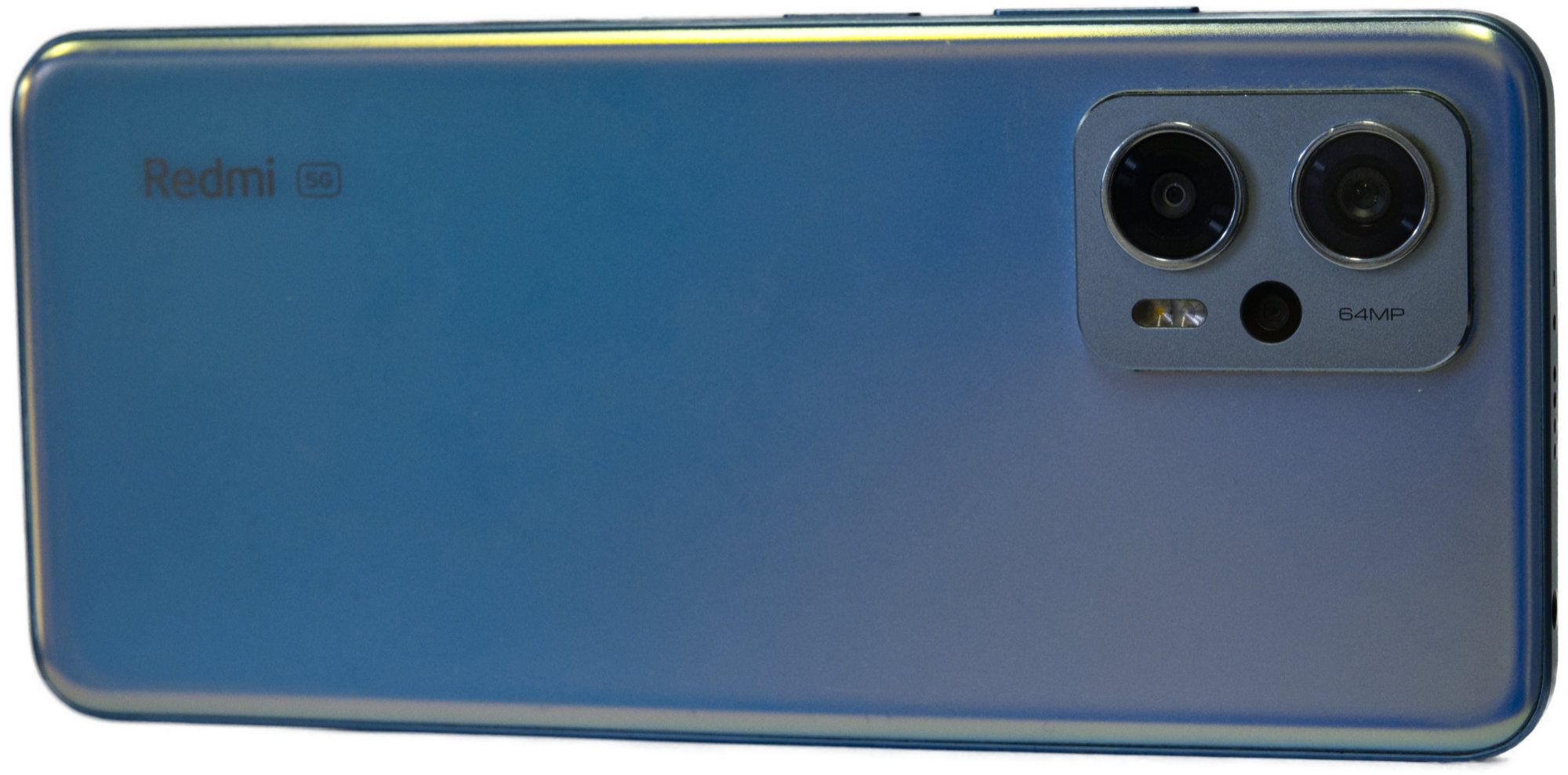
(d) width=0.4

Figure 11: Sensors employed for capturing the datasets.

VI-A3 Baselines

We compare our framework to both multi-view depth estimation (MVD) and incremental scene reconstruction (ISR) models.

For MVD, we compare with famous classic COLMAP [55, 56] and Deep learning based methods, such as MVSNet [33], Vis-MVSSNet [37], MVS2D [57], DeMon [28], DeepV2D [30], Robust MVD baseline [31], DUSt3R [42] and more. In particular, the latest fully supervised model DUSt3R [42] supports the closest to us. While ours is not a deep learning model.

For ISR, we include Dense RGB-D-SLAM SOTAs (NICE-SLAM [22], Vox-Fusion), Dense Mono-SLAM SOTAs (NeRF-SLAM, DROID-SLAM, NICER-SLAM), Surface Light Field model (NSLF-OL [15]).

VI-A4 Evaluation Metrics

In the MVD test, we follow RobustMVD [31] to use relative depth error and inlier ratio to metric the estimation quality. Since our model does not input both ground truth (GT) depth and inlier, for fair evaluation we follow DUSt3R [42] to align the depth to GT scale with median value.

In the ISR test, our evaluations are mainly for color, geometry, and pose. For color, we use PSNR, SSIM, and LPIPS. For geometry, we use accuracy, completion, and completion ratio. For trajectory, we use ATE RMSE. Before evaluating the geometry and trajectory, we follow NICER-SLAM to align the reconstruction and trajectories with the ICP tool of CloudCompare [58]. For the monocular scenario, scale is also corrected.

VI-B Effect of Multiview Detph Estimation

Methods		GT	GT	GT	Align	KITTI		ScanNet		ETH3D		DTU		T&T
		Pose	Range	Intrinsics		rel $\downarrow$	$\tau\uparrow$	rel $\downarrow$	$\tau\uparrow$	rel $\downarrow$	$\tau\uparrow$	rel $\downarrow$	$\tau\uparrow$	rel$\downarrow$	$\tau\uparrow$
(a)	COLMAP [55, 56]	$\checkmark$	$\times$	$\checkmark$	$\times$	12.0	58.2	14.6	34.2	16.4	55.1	0.7	96.5	2.7	95.0
	COLMAP Dense [55, 56]	$\checkmark$	$\times$	$\checkmark$	$\times$	26.9	52.7	38.0	22.5	89.8	23.2	20.8	69.3	25.7	76.4
(b)	MVSNet [33]	$\checkmark$	$\checkmark$	$\checkmark$	$\times$	22.7	36.1	24.6	20.4	35.4	31.4	(1.8)	$(86.0)$	8.3	73.0
	MVSNet Inv. Depth [33]	$\checkmark$	$\checkmark$	$\checkmark$	$\times$	18.6	30.7	22.7	20.9	21.6	35.6	(1.8)	$(86.7)$	6.5	74.6
	Vis-MVSSNet [37]	$\checkmark$	$\checkmark$	$\checkmark$	$\times$	9.5	55.4	8.9	33.5	10.8	43.3	(1.8)	(87.4)	4.1	87.2
	MVS2D ScanNet [57]	$\checkmark$	$\checkmark$	$\checkmark$	$\times$	21.2	8.7	(27.2)	(5.3)	27.4	4.8	17.2	9.8	29.2	4.4
	MVS2D DTU [57]	$\checkmark$	$\checkmark$	$\checkmark$	$\times$	226.6	0.7	32.3	11.1	99.0	11.6	(3.6)	(64.2)	25.8	28.0
(c)	DeMon [28]	$\checkmark$	$\times$	$\checkmark$	$\times$	16.7	13.4	75.0	0.0	19.0	16.2	23.7	11.5	17.6	18.3
	DeepV2D KITTI [30]	$\checkmark$	$\times$	$\checkmark$	$\times$	(20.4)	(16.3)	25.8	8.1	30.1	9.4	24.6	8.2	38.5	9.6
	DeepV2D ScanNet [30]	$\checkmark$	$\times$	$\checkmark$	$\times$	61.9	5.2	(3.8)	(60.2)	18.7	28.7	9.2	27.4	33.5	38.0
	MVSNet [33]	$\checkmark$	$\times$	$\checkmark$	$\times$	14.0	35.8	1568.0	5.7	507.7	8.3	(4429.1)	(0.1)	118.2	50.7
	MVSNet Inv. Depth [33]	$\checkmark$	$\times$	$\checkmark$	$\times$	29.6	8.1	65.2	28.5	60.3	5.8	(28.7)	(48.9)	51.4	14.6
	Vis-MVSNet [37]	$\checkmark$	$\times$	$\checkmark$	$\times$	10.3	54.4	84.9	15.6	51.5	17.4	(374.2)	(1.7)	21.1	65.6
	MVS2D ScanNet [57]	$\checkmark$	$\times$	$\checkmark$	$\times$	73.4	0.0	(4.5)	(54.1)	30.7	14.4	5.0	57.9	56.4	11.1
	MVS2D DTU [57]	$\checkmark$	$\times$	$\checkmark$	$\times$	93.3	0.0	51.5	1.6	78.0	0.0	(1.6)	(92.3)	87.5	0.0
	Robust MVD Baseline [31]	$\checkmark$	$\times$	$\checkmark$	$\times$	7.1	41.9	7.4	38.4	9.0	42.6	2.7	82.0	5.0	75.1
(d)	DeMoN [28]	$\times$	$\times$	$\checkmark$	$\|\mathbf{t}\|$	15.5	15.2	12.0	21.0	17.4	15.4	21.8	16.6	13.0	23.2
	DeepV2D KITTI [30]	$\times$	$\times$	$\checkmark$	med	(3.1)	(74.9)	23.7	11.1	27.1	10.1	24.8	8.1	34.1	9.1
	DeepV2D ScanNet [30]	$\times$	$\times$	$\checkmark$	med	10.0	36.2	(4.4)	(54.8)	11.8	29.3	7.7	33.0	8.9	46.4
	DUSt3R 224-NoCroCo [42]	$\times$	$\times$	$\times$	med	15.14	21.16	7.54	40.00	9.51	40.07	3.56	62.83	11.12	37.90
	DUSt3R 224 [42]	$\times$	$\times$	$\times$	med	15.39	26.69	(5.86)	(50.84)	4.71	61.74	2.76	77.32	5.54	56.38
	DUSt3R 512 [42]	$\times$	$\times$	$\times$	med	9.11	39.49	(4.93)	( 60.20)	2.91	76.91	3.52	69.33	3.17	76.68
	Ours	$\times$	$\times$	$\times$	med	2.08	82.01	7.19	22.17	1.87	50.14	15.61	33.74	2.46	81.00

TABLE I: Multi-view depth evaluation with different settings: a) Classical approaches; b) with poses and depth range, without alignment; c) absolute scale evaluation with poses, without depth range and alignment; d) without poses and depth range, but with alignment. (Parentheses) denote training on data from the same domain. The best results for each setting are in bold.

One of the most important components of SceneFactory is the depth estimator. We follow the Multiview Depth Estimation (MVD) benchmark, RobustMVD [31], to evaluate the depth result on 5 widely used datasets (KITTI, ScanNet, ETH3D, DTU, and Tanks&Temple). Because our model also support intrinsic-free, which is not listed in [31], so besides of the whole benchmark, we find DUSt3R [42] as the most similar work to follow for comparison.

VI-B1 Quantitative Evaluation

Please find Table I the benchmarking result. We follow DUSt3R [42] to add an additional column (GT Intrinsics) to indicate the requirement of intrinsics. Both ours and DUSt3R do not require GT pose, depth range, and intrinsics. First, on the indoor and outdoor datasets ETH3D, Tanks&Temple and KITTI, our model outperforms performs best on all (a-d) folds.

On the indoor dataset ScanNet, our model does not outperform DUSt3R. This is because ScanNet was originally acquired for RGB-D SLAM, which contains large rotation and small translation. The reference and source images do not have a good triangulation relationship. The other thing is that ScanNet’s image contains strong motion blur, which is harmful to dense matching based models like our model. Nevertheless, our model still outperforms the matching-based baseline, RobustMVD.

At the object level, our model performs particularly poorly on the DTU dataset. We believe this is because in our model, none of the optical flow, monodepth, or deep covariance is trained on the object.

While differently, DUSt3R requires training on eight indoor&outdoor dataset, which includes indoor, outdoor, synthetic, real-world, object-centric and more.

Our model relies on dense bundle adjustment, which we consider is less affected by the deep prior.

Therefore, from a practical point of view, DUSt3R 1) is not guaranteed to work on custom scene dataset (will be shown in Section VI-B3), 2) DUSt3R is not able to work with given poses and intrinsics. These are not a problem for our model and allow us to work with our entire SceneFactory pipeline.

VI-B2 Qualitative Evaluation

We show the estimated depth and error in Fig. 12 next to the Table I. Where we have attached the robustMVD’s qualitative result of the $5$ dataset in Table I sequentially.

Please find in figure that our result has better performance on outdoor and indoor dataset except for ScanNet. Which we consider is because of the nature of our method of dense matching. while ScanNet contains strong motion blur caused by quite old RGB camera. However, DUSt3R is more with monodepth because during the benchmarking, DUSt3R does not benefit from more source views. So is not affected by this issue.

Although our average score on object dataset DTU is lower, but it is because our method fail on some cases. While the robustMVD selected qualitative figure is still better.

Ref-RGB	DUSt3R-MVD	DUSt3R-absrel	Ours-MVD	Ours-absrel

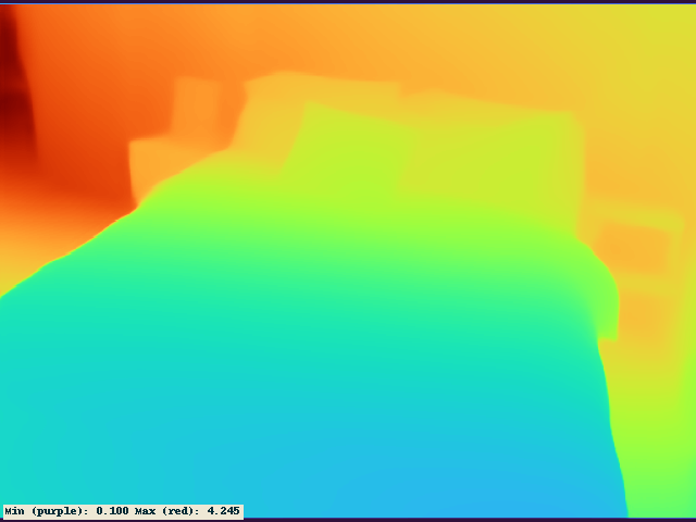
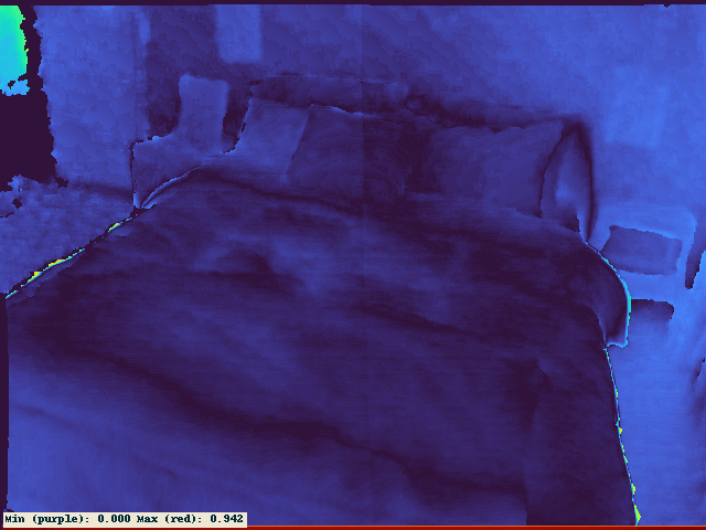
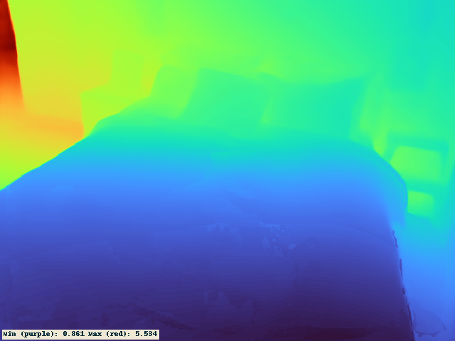
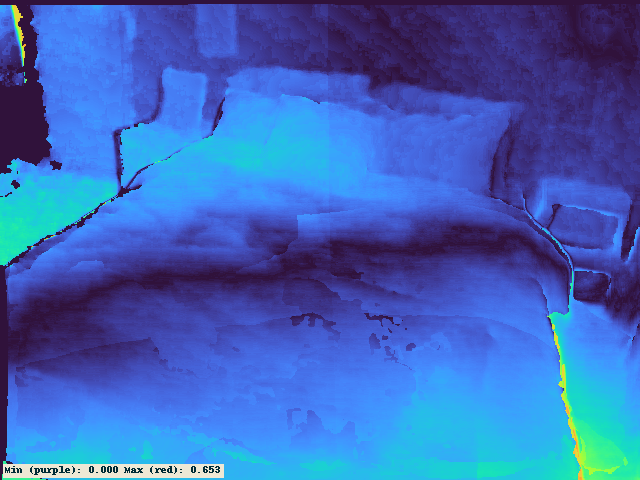
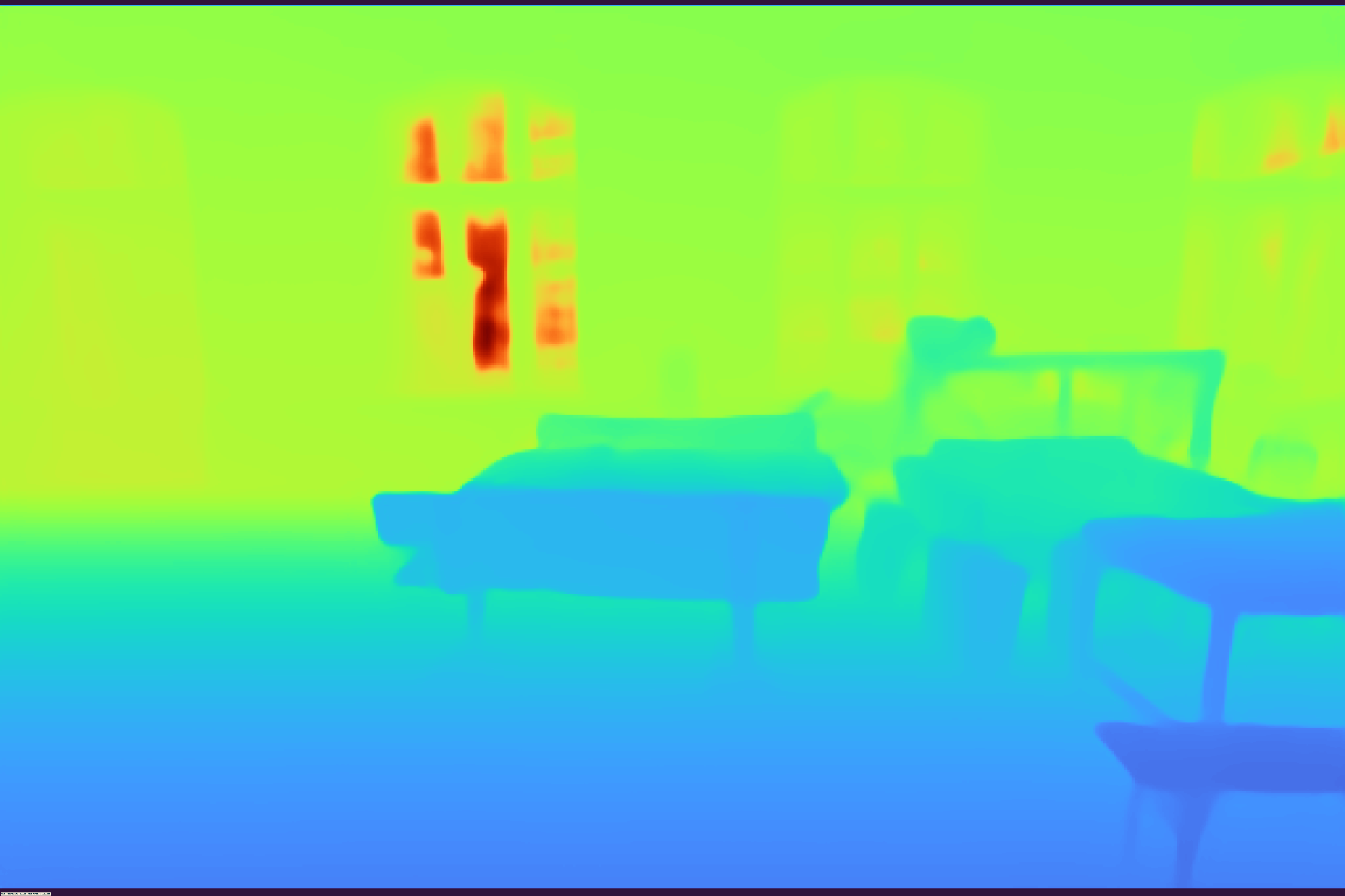
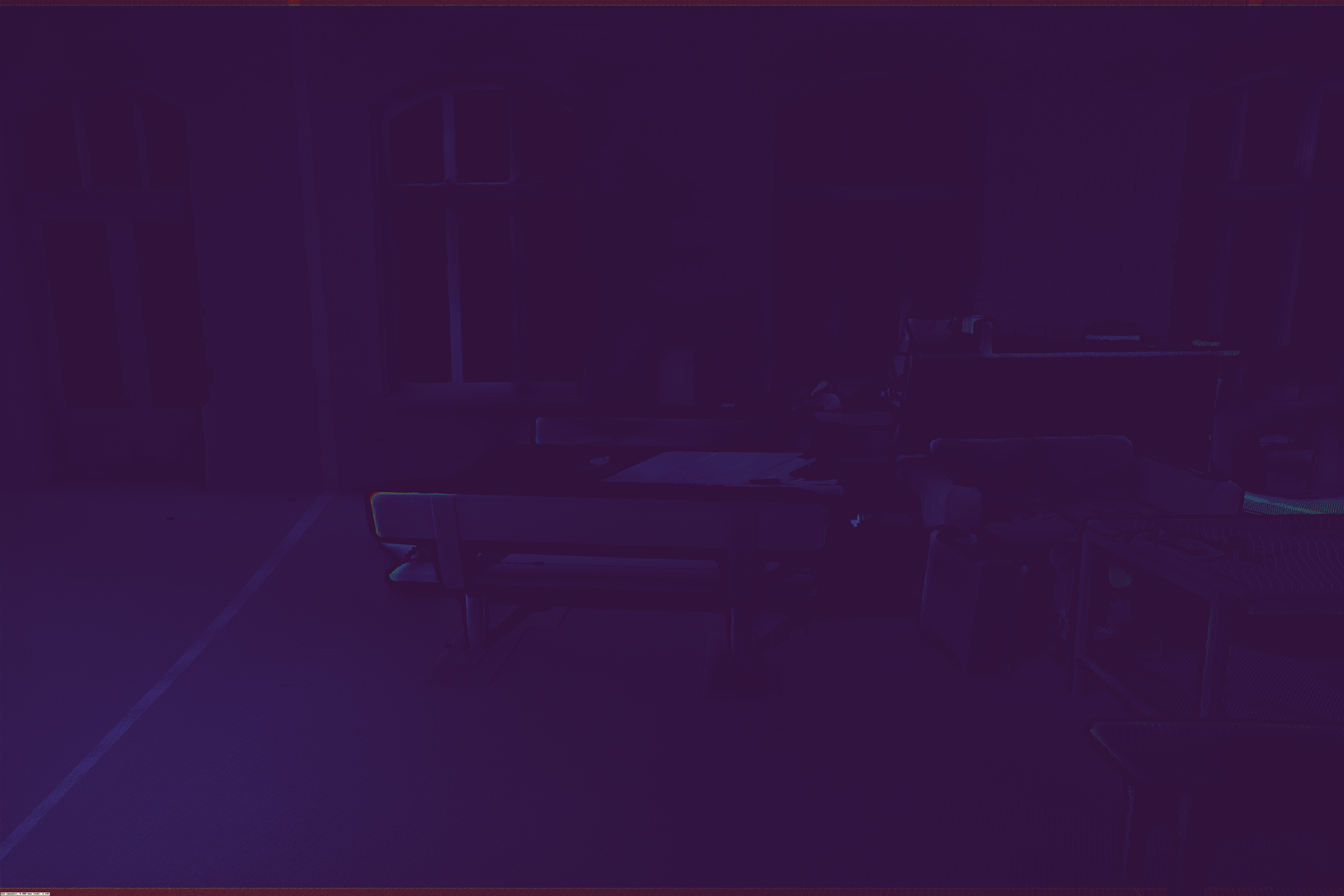
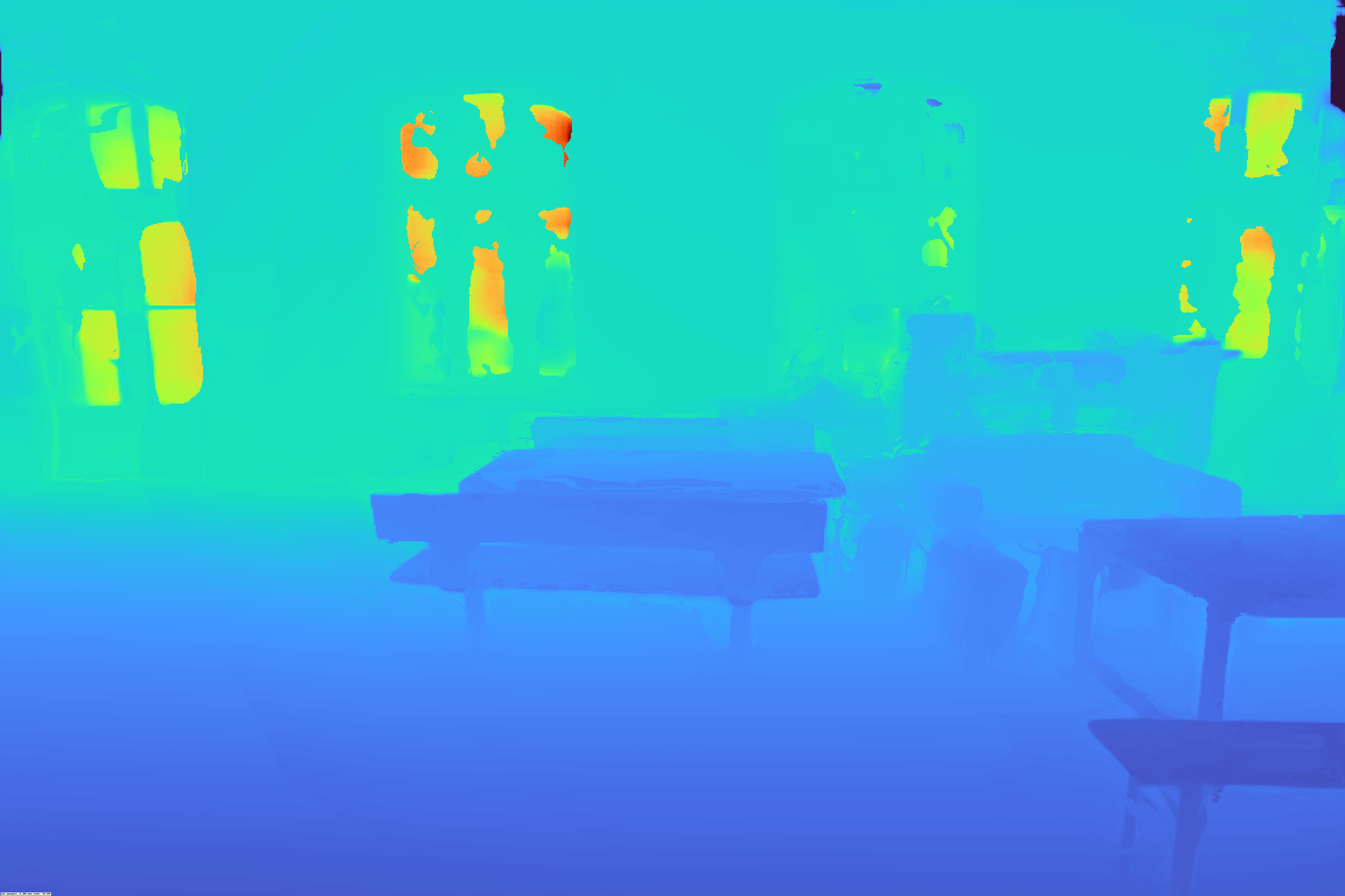
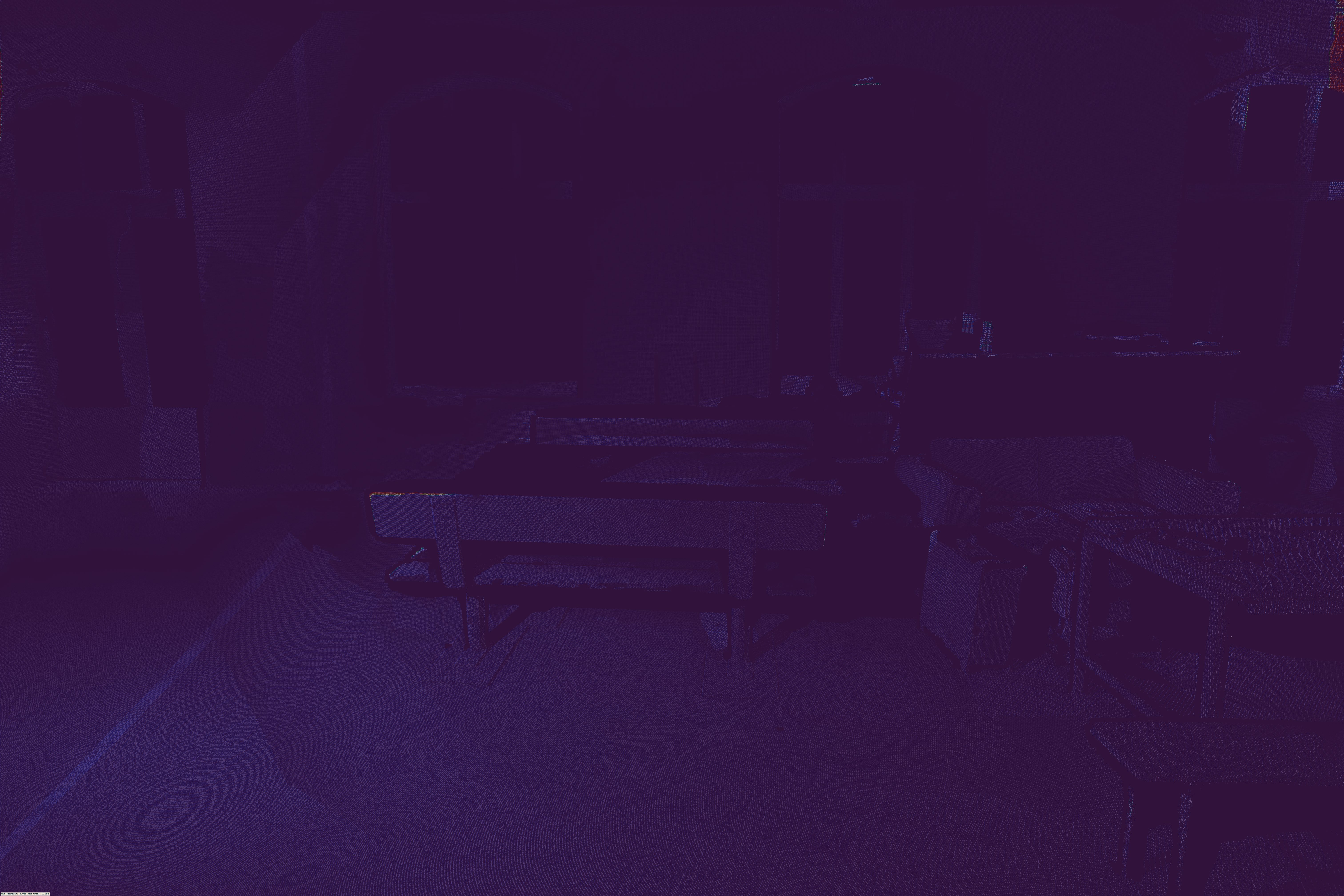
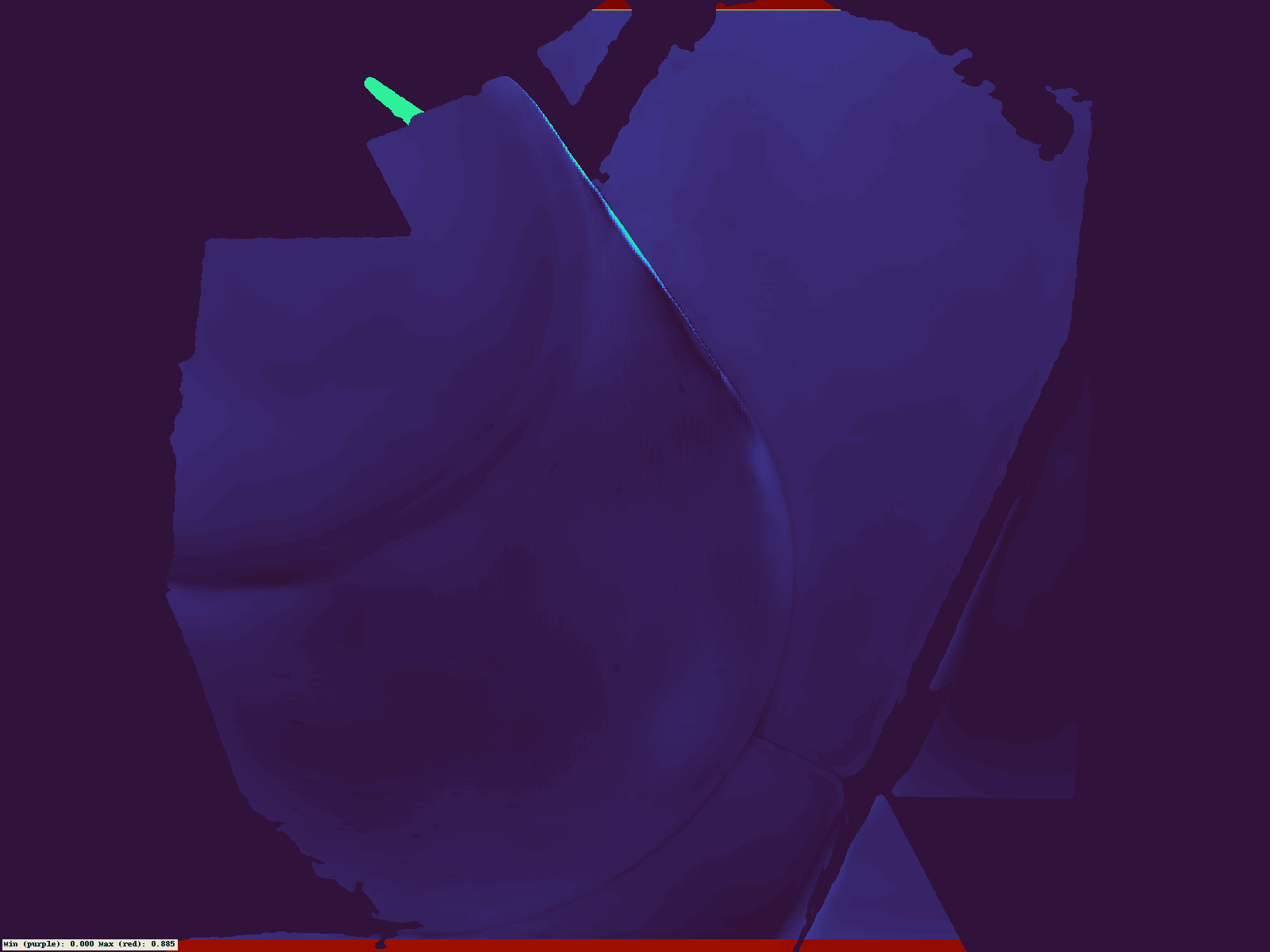
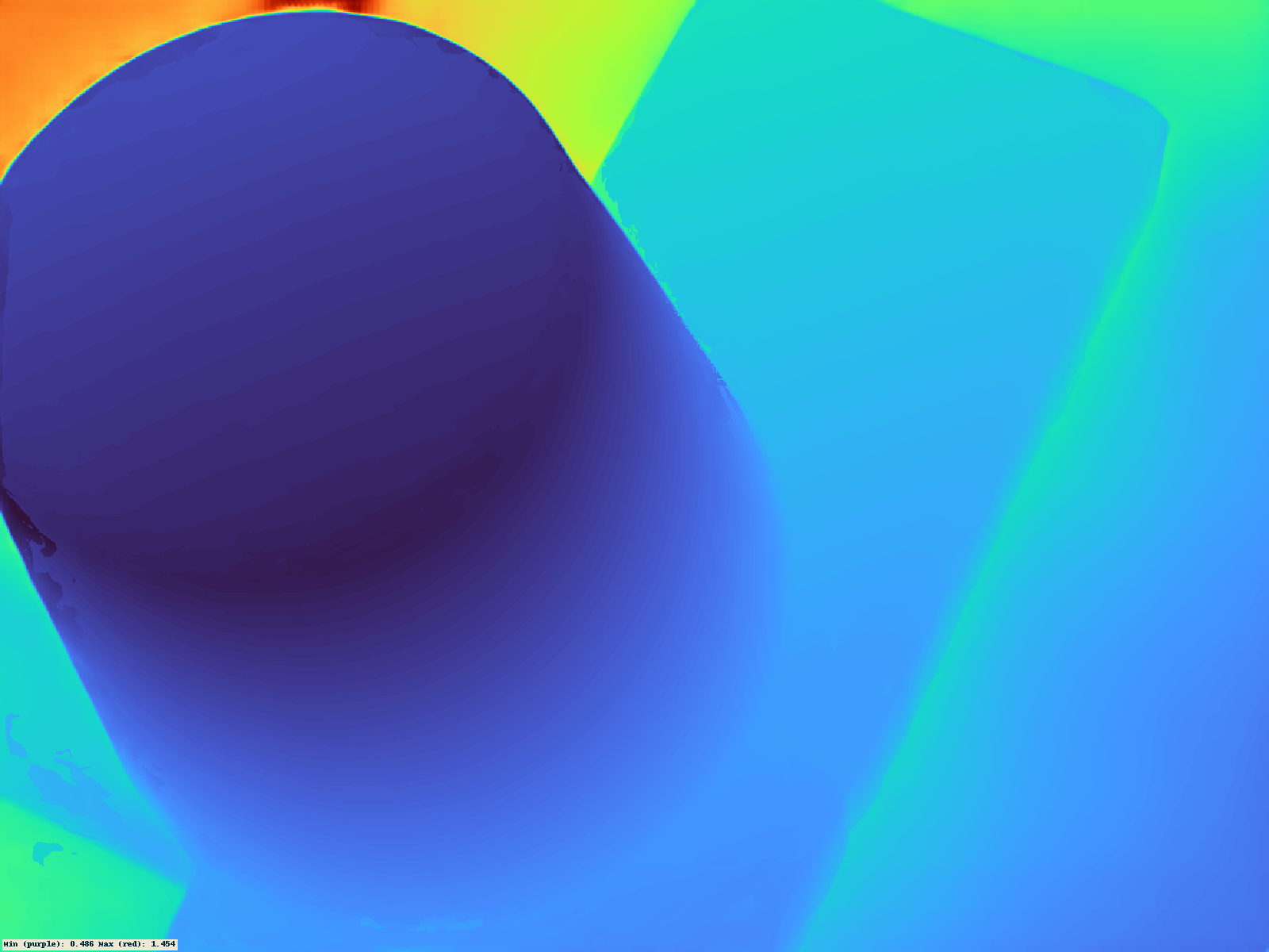
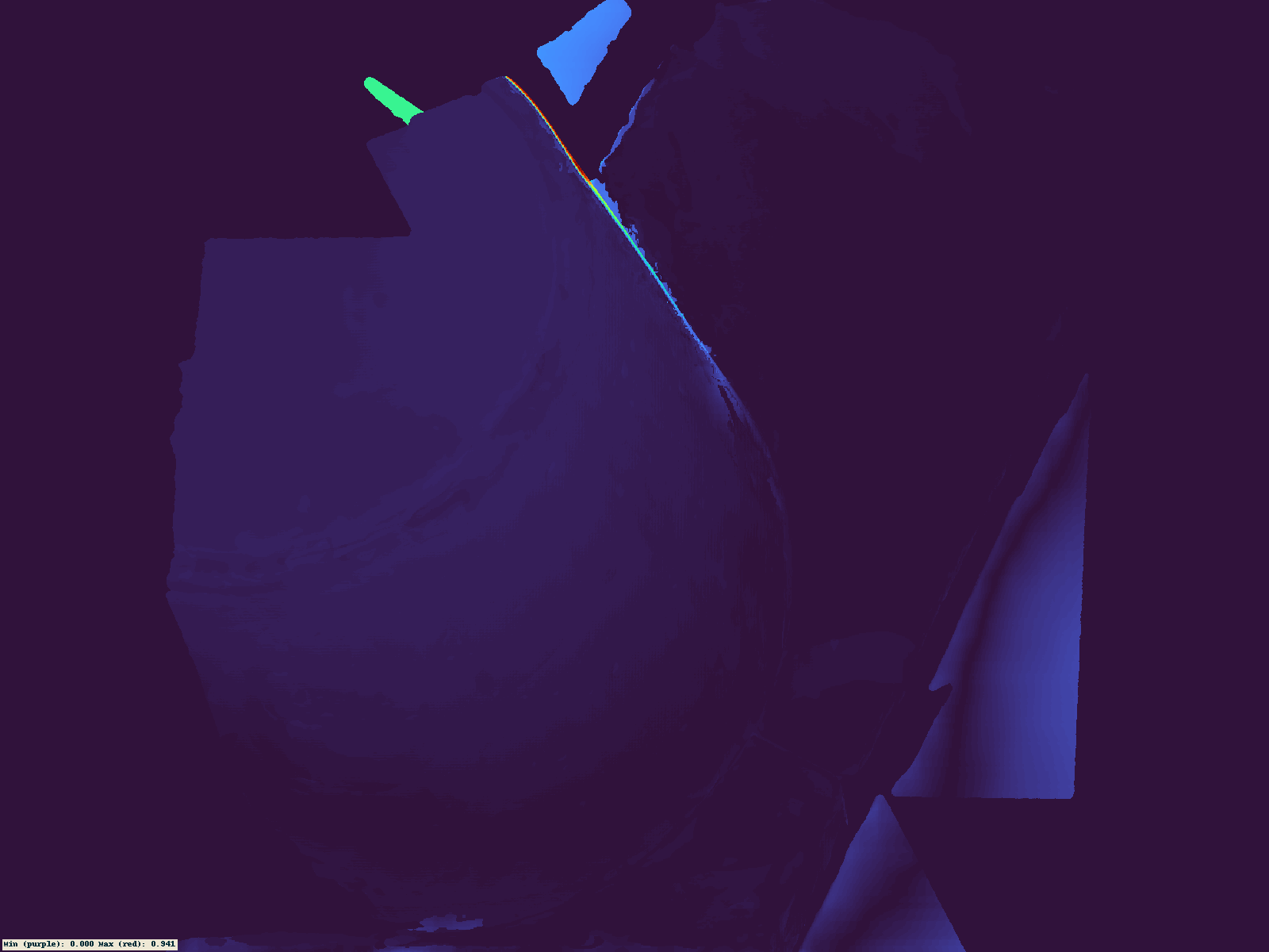
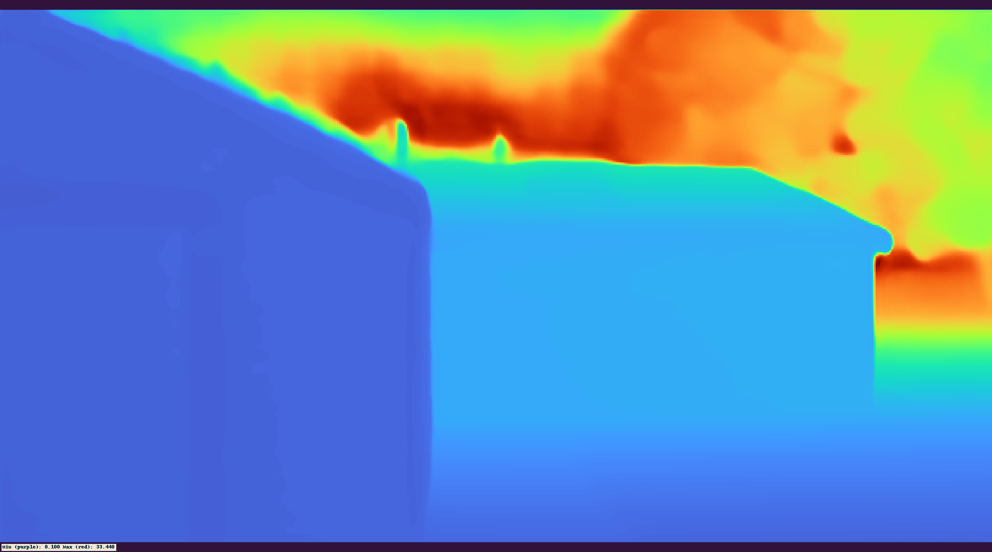
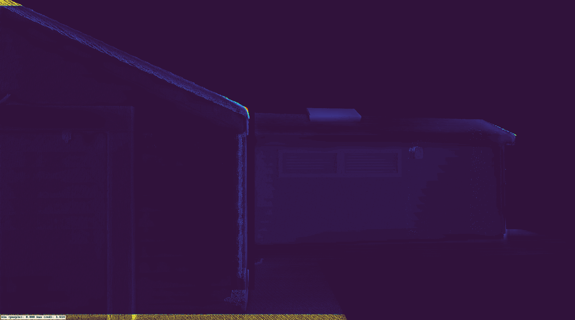
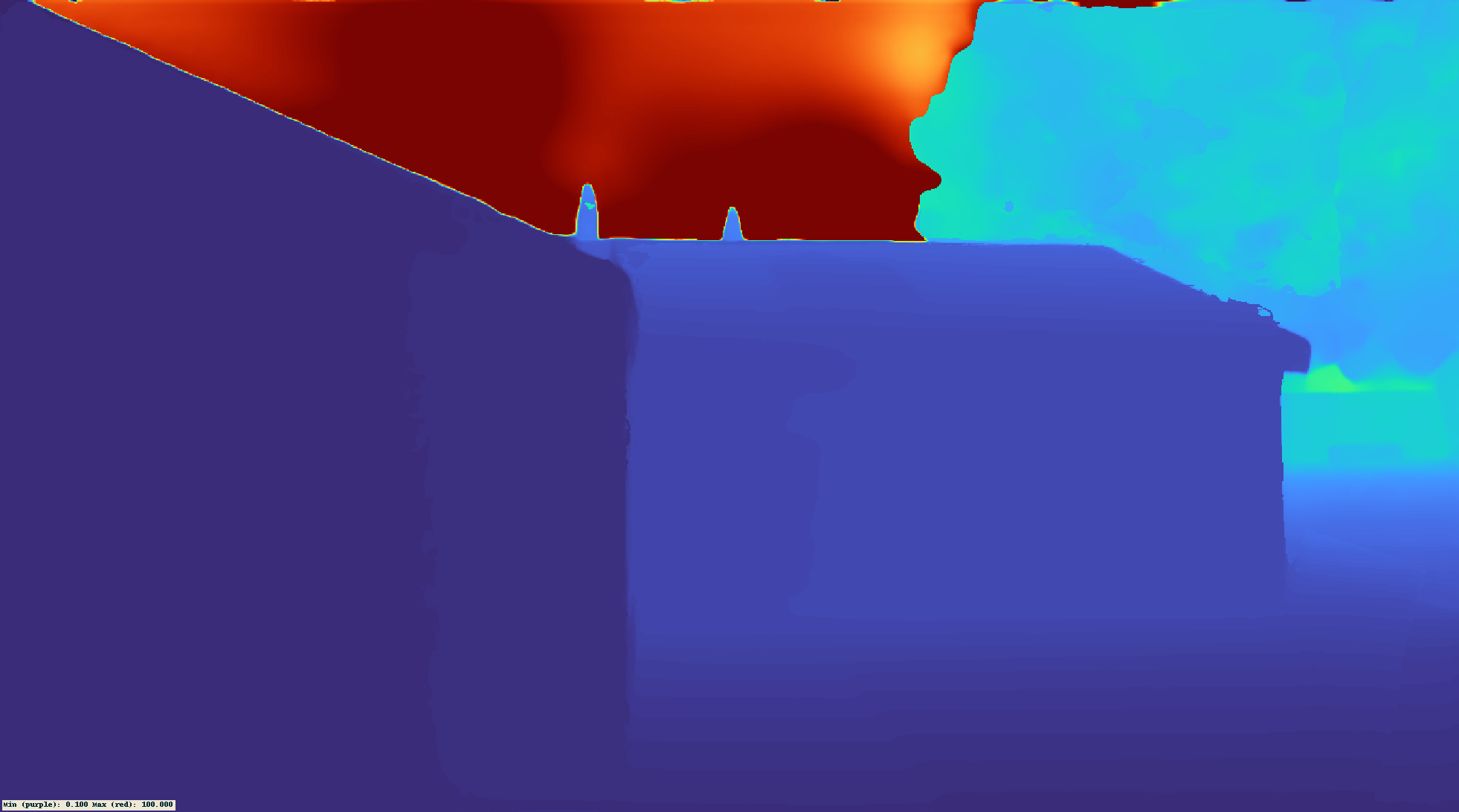
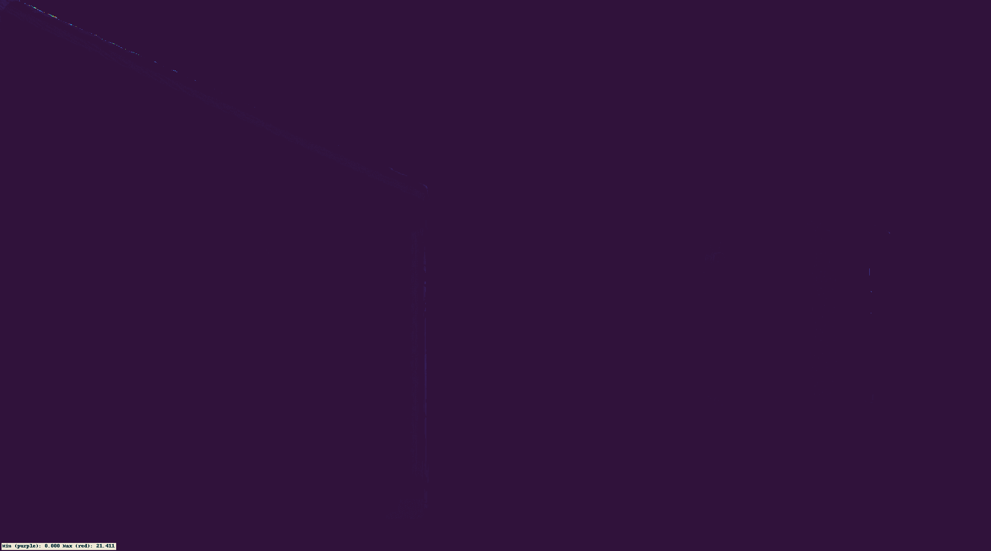
Figure 12: Result of MVD.

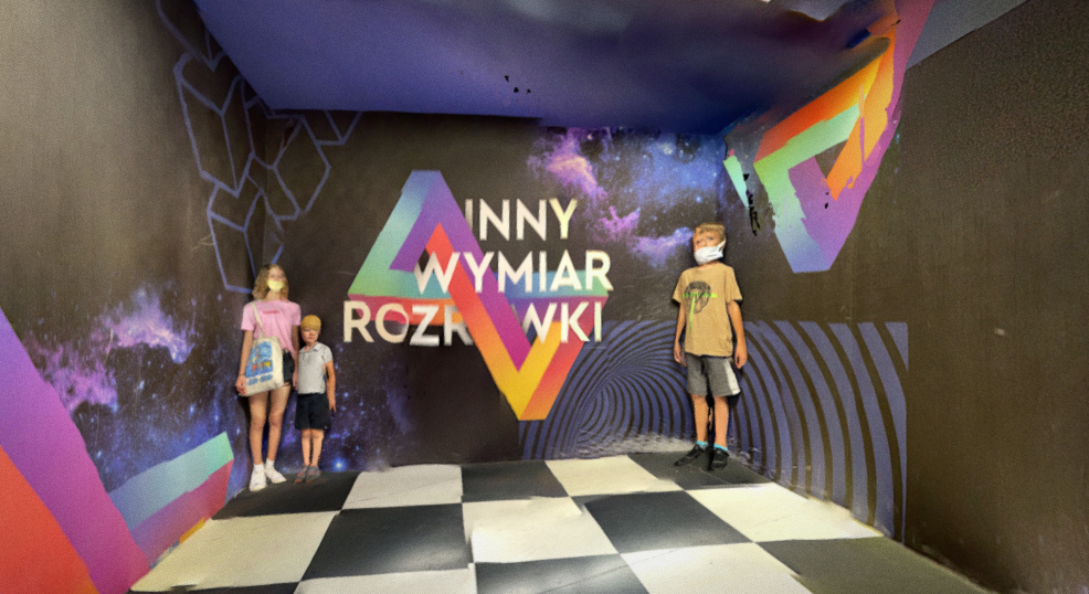
(a) width=.5

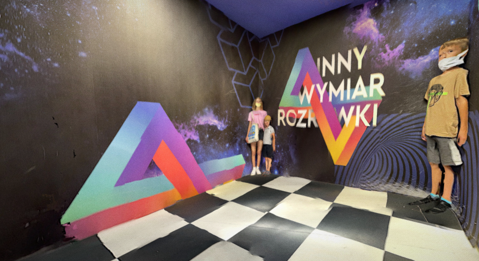
(b) width=.5

Figure 13: MVS input of Ames room. The true shape please find webpage ${}^{4}$.

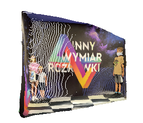
(a) width=.5

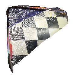
(b) width=.4

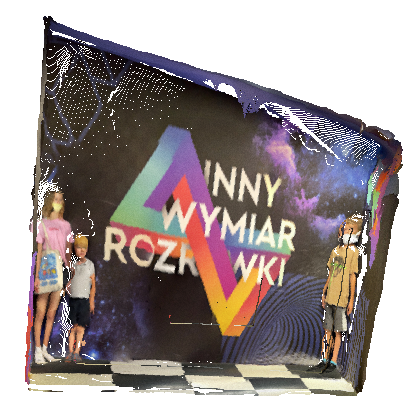
(c) width=.5

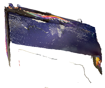
(d) width=.5

Figure 14: MVD on Ames room. The true shape please find webpage ${}^{4}$.

VI-B3 Demonstration on Custom Data

As we claimed earlier, DUSt3R is not guaranteed to work due to the limitation of the training dataset. In addition, due to the fact that 1) DUSt3R does not improve with increasing number of source images in the RobustMVD benchmark and 2) performs similarly with and without source images. We suggest that the SOTA DUSt3R is mainly based on its strength of monocular depth.

To verify this, we test on the vision illusion that also happens to a human eye vision, the Ames Room. Here we show the data of the Ames Room in Fig. 13. Where we capture the image from Sketchfab resource Ames Room to create the illusion of a distorted room. Where typically shows incorrect relative scales on the left and right corners. DUSt3R, as we suspected, shows the Ames space as a normal space, as in Fig. 14. While our model, on the contrary, really reproduces the distorted room.

Therefore, our MVD shows similar or even better MVD performance and a much more reliable result.

TABLE II: Full model comparison on Replica sequences. Header indicates scene names.

		Office0	Office1	Office2	Office3	Office4	Room0	Room1	Room2
NICE-SLAM [22]	PSNR $\uparrow$	28.38	30.68	23.90	24.88	25.18	23.46	23.97	25.94
	SSIM $\uparrow$	0.908	0.935	0.893	0.888	0.902	0.798	0.838	0.882
	LPIPS $\downarrow$	0.386	0.278	0.330	0.287	0.326	0.443	0.401	0.315
Surface Light Field methods
NSLF-OL[15]+DI-Fusion[16]	PSNR $\uparrow$	28.59	26.70	21.10	21.89	25.74	23.24	25.68	24.88
	SSIM $\uparrow$	0.913	0.879	0.863	0.847	0.893	0.816	0.883	0.888
	LPIPS $\downarrow$	0.371	0.497	0.362	0.368	0.401	0.371	0.308	0.330
SceneFactory (Ours)	PSNR $\uparrow$	33.38	31.89	24.84	25.39	31.14	27.98	29.51	30.64
	SSIM $\uparrow$	0.921	0.893	0.837	0.873	0.893	0.858	0.883	0.898
	LPIPS $\downarrow$	0.167	0.267	0.208	0.129	0.178	0.111	0.149	0.145

NSLF-OL	SceneFactory	Ground Truth

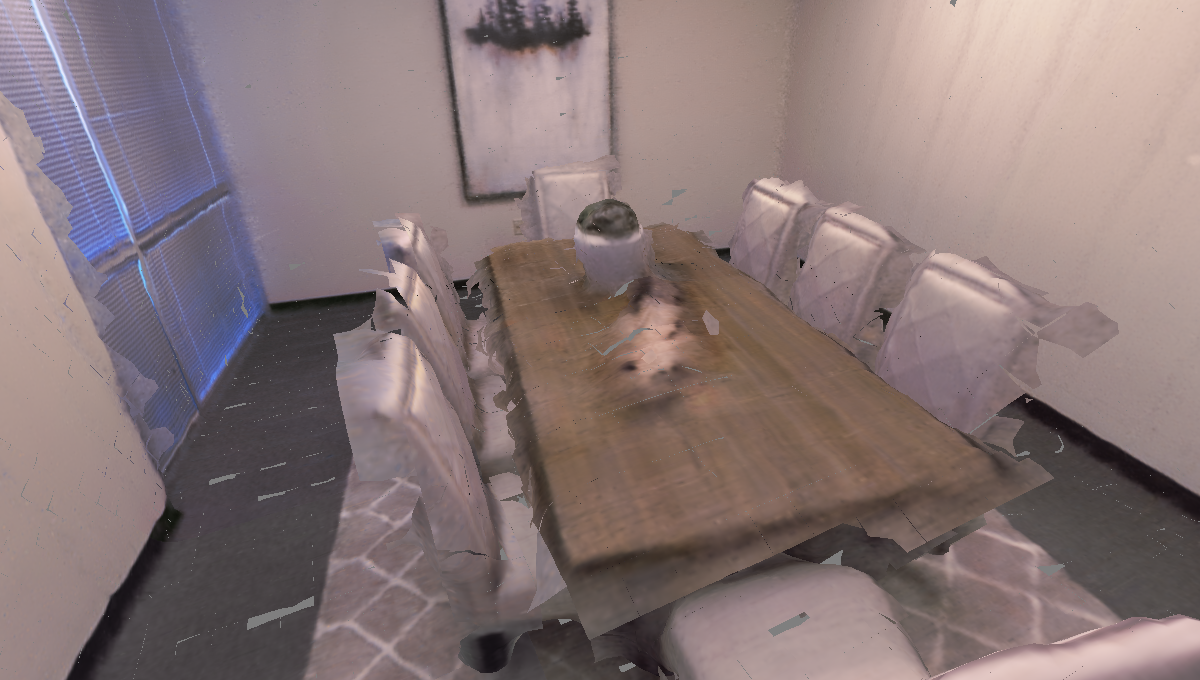
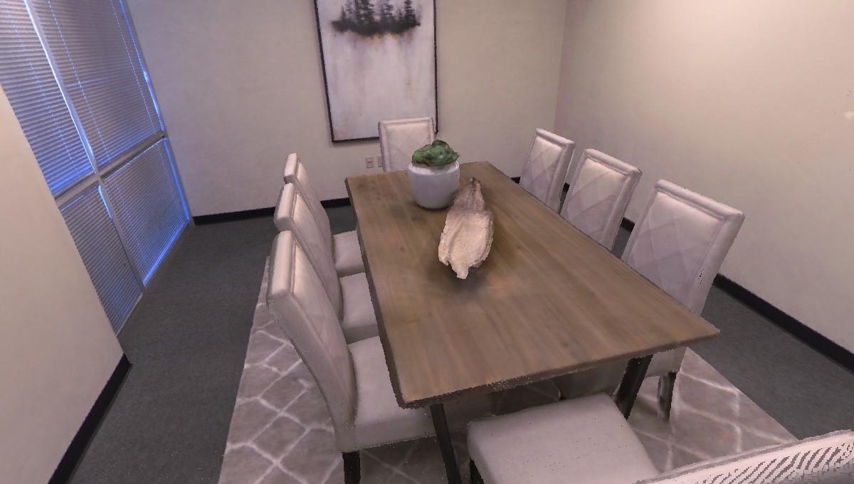
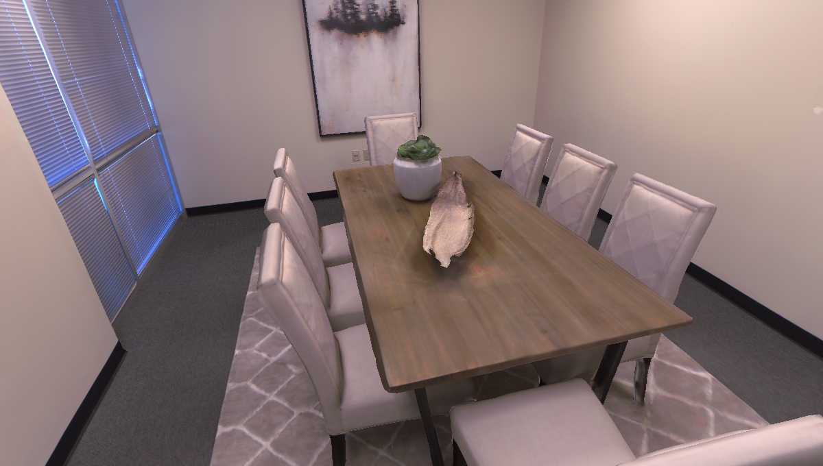
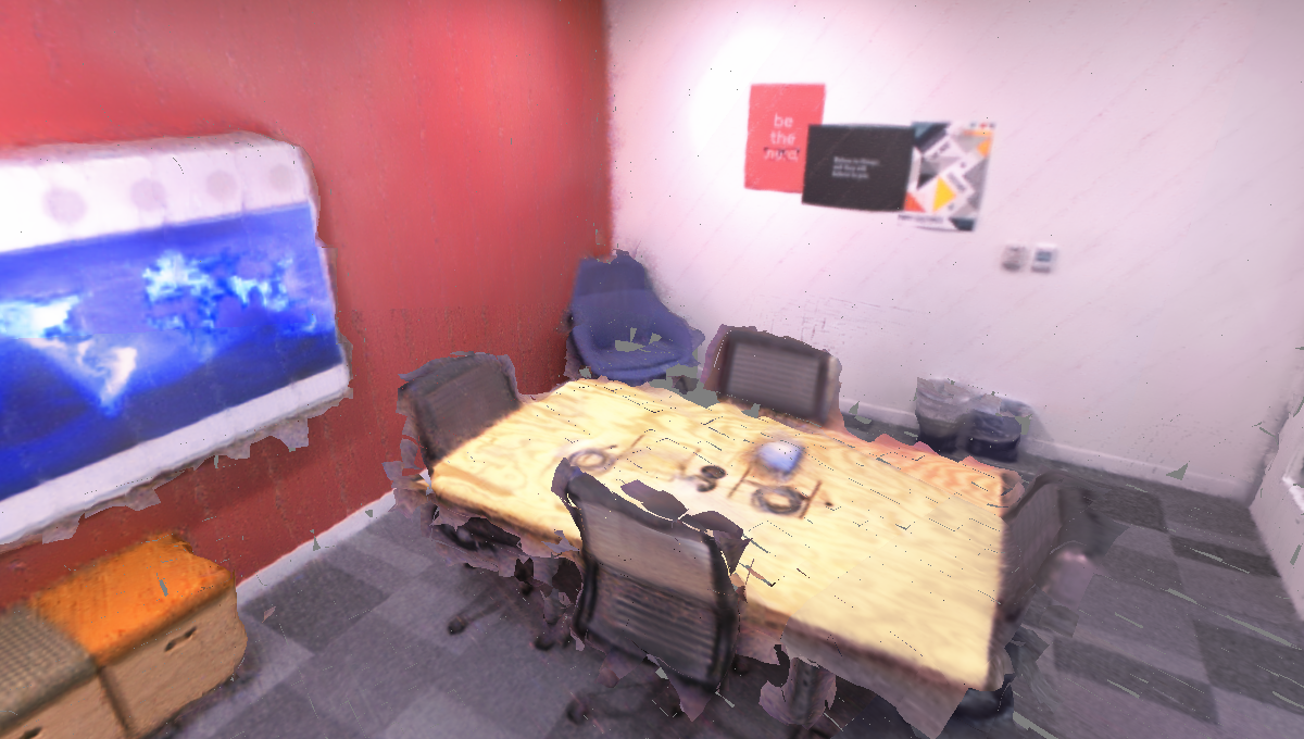
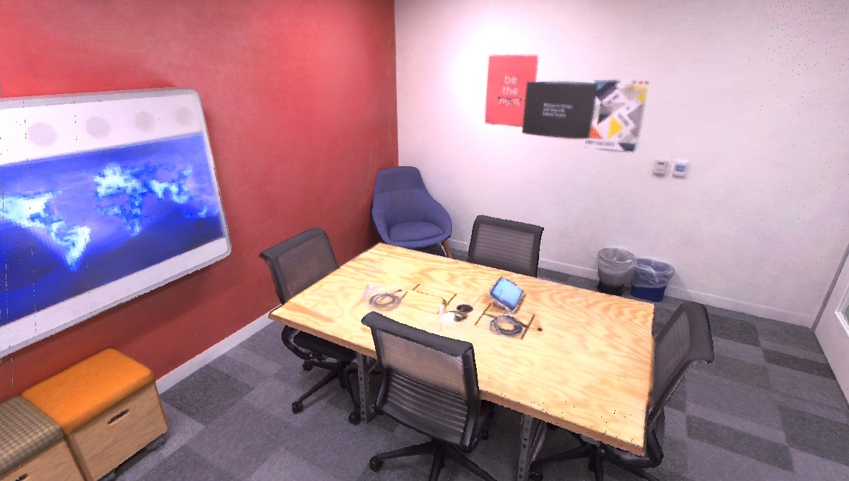
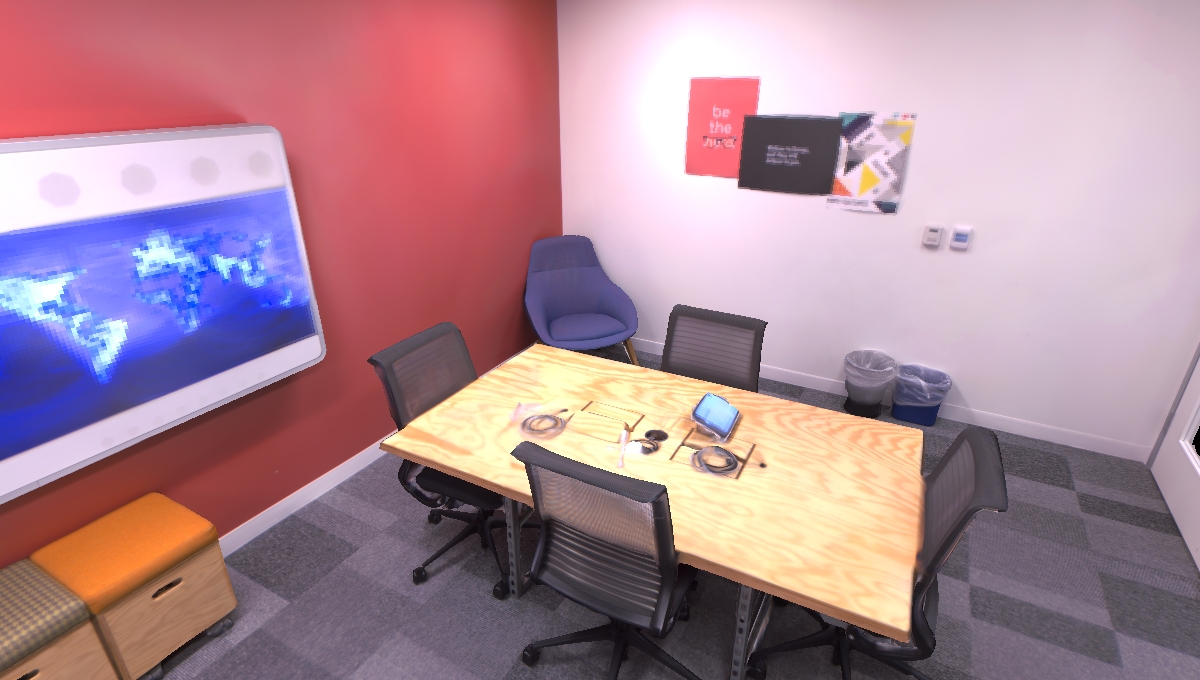
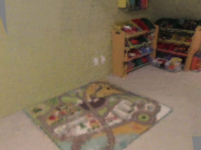
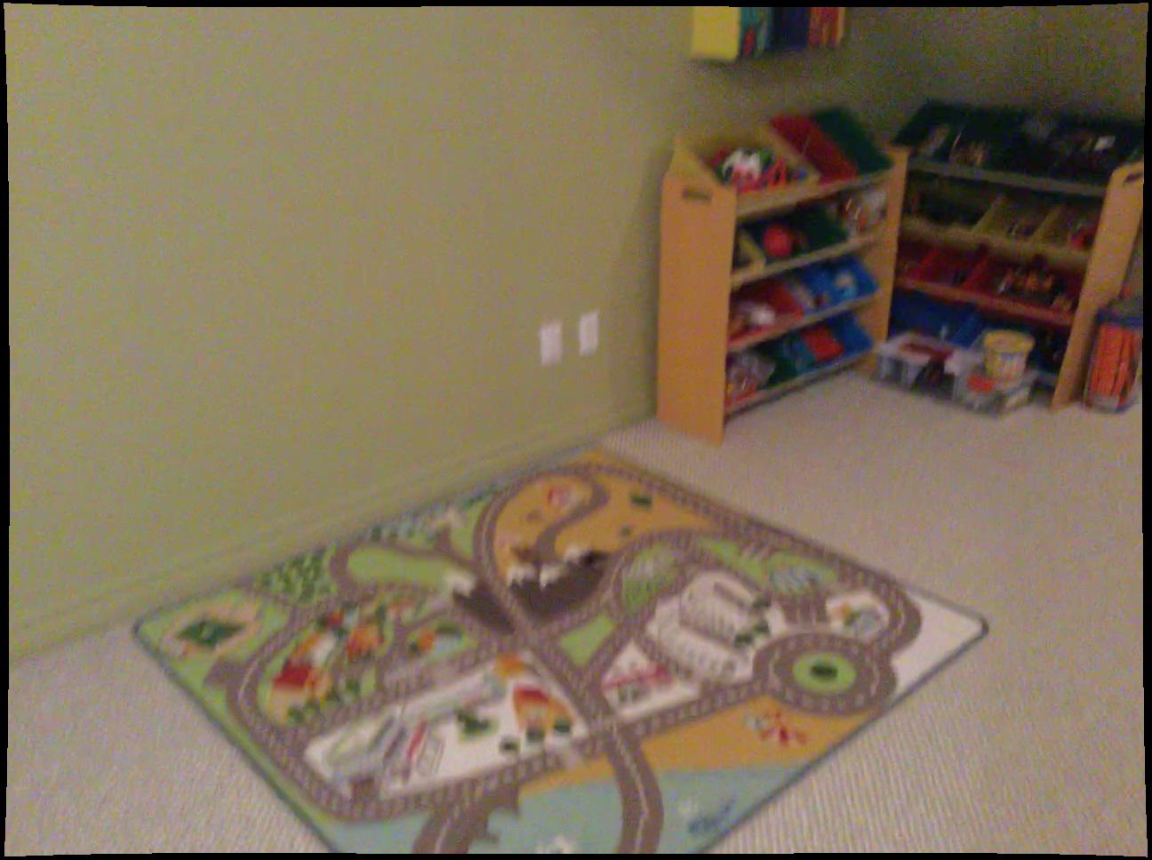
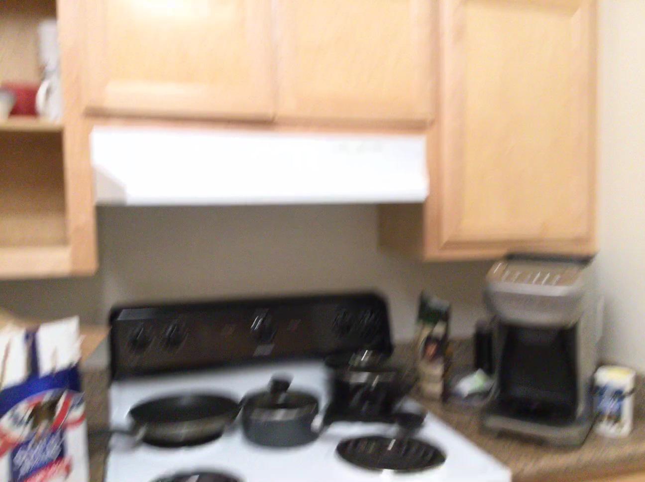
Figure 15: Result of Surface Light Field test on Replica and ScanNet dataset.

VI-C Evaluation on Surface Light Fields (SLF)

In the test above, we generate depth from images. In this subsection, we generate a color image and explore the importance of our surface light field model.

VI-C1 Replica Test

To mitigate the effects of other SceneFactory blocks, image, depth, pose and intrinsics $(\mathbf{I}_{rgb},\mathbf{I}_{d},\mathbf{G},\mathbf{\theta})$ are all available in the dependency graph ( Fig. 2).

First, we follow the scene-level SLF model NSLF-OL [15] to test on the replica dataset. From Table II, our model strongly outperforms the NICE-SLAM and SOTA SLF model, NSLF-OL on all PSNR, SSIM, LPIPS metrics. To make the comparison more obvious, we show images in the Fig. 15, the first two rows are from the Replica dataset. From this, we can see that the main advances of our model are that on the one hand, unlike NSLF-OL, our DM-NPs itself can provide a cleaner surface, and on the other hand, our SLF recovers the color better. Also, NSLF-OL only works alongside the surface model, while our SLF model can support surface generation by itself.

We demonstrate the result images in Fig. 15 the row $1,2$. Where it shows better color rendering.

VI-C2 ScanNet Test

TABLE III: Surface Light Field comparison on ScanNet sequences.

		0568	0164
NSLF-OL +Di-Fusion	PSNR $\uparrow$	19.09	18.78
	SSIM $\uparrow$	0.500	0.595
	LPIPS $\downarrow$	0.575	0.551
SceneFactory	PSNR $\uparrow$	19.90	21.85
	SSIM $\uparrow$	0.573	0.688
	LPIPS $\downarrow$	0.536	0.444

Following the same setup, we continue testing on ScanNet. Please find Fig. 15. The ScanNet image has a lot of blur on the image and more noise in the depth (due to the low quality capture).

However, our result is still better than NSLF-OL with better quantitative evaluation (Table III). From the image shown in Fig. 15 the row $3,4$, we can see that the structure of NSLF-OL is not well reconstructed. Our result is much clearer.

VI-D Evaluation of Dense SLAM

In this section, we evaluate SceneFactory’s main application, Dense SLAM, in both RGB-D and monocular settings after SOTA NICER SLAM.

VI-D1 Replica Test

TABLE IV: Camera Tracking Results on the Replica Dataset. ATE RMSE [cm] ($\downarrow$) is used as the evaluation metric.

	rm-0	rm-1	rm-2	off-0	off-1	off-2	off-3	off-4	Avg.
RGB-D input
NICE-SLAM	1.69	2.04	1.55	0.99	0.90	1.39	3.97	3.08	1.95
Vox-Fusion	0.27	1.33	0.47	0.70	1.11	0.46	0.26	0.58	0.65
SceneFactory	0.20	0.12	0.14	0.17	0.07	0.13	0.29	0.22	0.17
RGB input
COLMAP	0.62	23.7	0.39	0.33	0.24	0.79	0.14	1.73	3.49
NeRF-SLAM	17.26	11.94	15.76	12.75	10.34	14.52	20.32	14.96	14.73
DIM-SLAM	0.48	0.78	0.35	0.67	0.37	0.36	0.33	0.36	0.46
DROID-SLAM	0.34	0.13	0.27	0.25	0.42	0.32	0.52	0.40	0.33
NICER-SLAM	1.36	1.60	1.14	2.12	3.23	2.12	1.42	2.01	1.88
SceneFactory	0.20	0.20	0.15	0.20	0.12	0.25	0.29	0.22	0.20

First, we follow Dense Mono-SLAM SOTA, NICER-SLAM, to have a complete test on both color and geometric on Replica dataset.

We show the tracking performance, from Table IV, SceneFactory achieves the best tracking performance overall. While with RGB input, SceneFactory uses Momo-SLAM DPVO, but with RGB-D input, SceneFactory uses our generalized DPVO with RGB-D, which achieves the best performance.

Notably, with RGB and depth as input, NSLF-OL requires an external reconstruction model to provide the surface prediction. While in contrast, SceneFactory itself also supports surface. We render inputted frames for depth and accumulate a point cloud. To fit in the evaluation script of NICER-SLAM, we extract mesh via Screened Poisson Surface Reconstruction for the evaluation. Table V shows the performance of the reconstruction. In addition, to demonstrate the ability to reconstruct surface color, we show the color result in Table V in the view synthesis comparison. The upper rows are with RGB-D input, while the lower rows are with RGB input.

From the tables, we can see that with RGB-D input, SceneFactory outperforms all SOTAs in both reconstruction and view generation over all scenes by a wide margin. To better demonstrate the quality, we show a qualitative evaluation in Fig. 16. Here our method works best. Please find the high detailed texture on the quilt.

TABLE V: Reconstruction Results on the Replica dataset. Best results are highlighted as first, second, and third.

		rm-0	rm-1	rm-2	off-0	off-1	off-2	off-3	off-4	Avg.
RGB-D input
NICE	Acc.[cm]$\downarrow$	3.53	3.60	3.03	5.56	3.35	4.71	3.84	3.35	3.87
	Comp.[cm]$\downarrow$	3.40	3.62	3.27	4.55	4.03	3.94	3.99	4.15	3.87
	Comp.Ratio[$<\!5$cm %]$\uparrow$	86.05	80.75	87.23	79.34	82.13	80.35	80.55	82.88	82.41
Vox-Fusion	Acc.[cm]$\downarrow$	2.53	1.69	3.33	2.20	2.21	2.72	4.16	2.48	2.67
	Comp.[cm]$\downarrow$	2.81	2.51	4.03	8.75	7.36	4.19	3.26	3.49	4.55
	Comp.Ratio[$<\!5$cm %]$\uparrow$	91.52	91.34	86.78	81.99	82.03	85.45	87.13	86.53	86.59
Ours	Acc.[cm]$\downarrow$	1.49	1.16	1.24	1.11	0.91	1.37	1.62	1.52	1.30
	Comp.[cm]$\downarrow$	3.65	2.88	4.31	1.68	2.23	3.59	3.59	4.02	3.24
	Comp.Ratio[$<\!5$cm %]$\uparrow$	87.61	90.02	86.83	93.43	90.39	86.24	84.98	85.07	88.07
RGB input
NeRF-S.	Acc. [cm]$\downarrow$	11.84	10.62	11.86	9.32	14.40	11.54	16.31	11.11	12.13
	Comp. [cm]$\downarrow$	5.63	5.88	9.22	13.29	10.17	6.95	7.81	5.26	8.03
	Comp. Ratio [%]$\uparrow$	61.13	68.19	47.85	37.64	56.17	66.20	55.67	61.86	56.84
DROID-S.	Acc. [cm]$\downarrow$	12.18	8.35	3.26	3.01	2.39	5.66	4.49	4.65	5.50
	Comp. [cm]$\downarrow$	8.96	6.07	16.01	16.19	16.20	15.56	9.73	9.63	12.29
	Comp. Ratio [%]$\uparrow$	60.07	76.20	61.62	64.19	60.63	56.78	61.95	67.51	63.60
NICER-S.	Acc. [cm]$\downarrow$	2.53	3.93	3.40	5.49	3.45	4.02	3.34	3.03	3.65
	Comp. [cm]$\downarrow$	3.04	4.10	3.42	6.09	4.42	4.29	4.03	3.87	4.16
	Comp. Ratio [%]$\uparrow$	88.75	76.61	86.1	65.19	77.84	74.51	82.01	83.98	79.37
Ours	Acc. [cm]$\downarrow$	3.61	4.02	5.53	2.71	2.17	4.09	4.23	3.69	3.76
	Comp. [cm]$\downarrow$	6.98	6.76	12.24	6.46	5.59	10.31	7.53	10.46	8.29
	Comp. Ratio [%]$\uparrow$	74.06	72.59	63.85	77.80	75.26	65.56	68.89	69.10	70.89

TABLE VI: Novel View Synthesis Evaluation on Replica Dataset. Best results are highlighted as first, second, and third.

		rm-0	rm-1	rm-2	off-0	off-1	off-2	off-3	off-4	Avg.
RGB-D input
NICE-S.	PSNR $\uparrow$	22.12	22.47	24.52	29.07	30.34	19.66	22.23	24.94	24.42
	SSIM $\uparrow$	0.689	0.757	0.814	0.874	0.886	0.797	0.801	0.856	0.809
	LPIPS $\downarrow$	0.330	0.271	0.208	0.229	0.181	0.235	0.209	0.198	0.233
Vox-F.	PSNR $\uparrow$	22.39	22.36	23.92	27.79	29.83	20.33	23.47	25.21	24.41
	SSIM $\uparrow$	0.683	0.751	0.798	0.857	0.876	0.794	0.803	0.847	0.801
	LPIPS $\downarrow$	0.303	0.269	0.234	0.241	0.184	0.243	0.213	0.199	0.236
Ours	PSNR $\uparrow$	27.72	28.86	30.17	32.59	31.39	24.44	25.34	30.47	28.87
	SSIM $\uparrow$	0.850	0.872	0.899	0.915	0.892	0.837	0.867	0.887	0.877
	LPIPS $\downarrow$	0.124	0.166	0.143	0.165	0.262	0.208	0.132	0.184	0.173
RGB input
NeRF-S.	PSNR $\uparrow$	16.45	19.62	21.17	21.44	20.86	15.49	15.11	18.96	18.64
	SSIM $\uparrow$	0.576	0.700	0.754	0.773	0.747	0.731	0.688	0.790	0.720
	LPIPS $\downarrow$	0.330	0.177	0.170	0.335	0.229	0.251	0.282	0.241	0.252
DROID-S.	PSNR $\uparrow$	21.41	24.04	22.08	23.59	21.29	20.64	20.22	20.22	21.69
	SSIM $\uparrow$	0.693	0.786	0.826	0.868	0.863	0.828	0.808	0.819	0.812
	LPIPS $\downarrow$	0.329	0.270	0.228	0.232	0.207	0.231	0.234	0.237	0.246
NICER-S.	PSNR $\uparrow$	25.33	23.92	26.12	28.54	25.86	21.95	26.13	25.47	25.41
	SSIM $\uparrow$	0.751	0.771	0.831	0.866	0.852	0.820	0.856	0.865	0.827
	LPIPS $\downarrow$	0.250	0.215	0.176	0.172	0.178	0.195	0.162	0.177	0.191
Ours	PSNR $\uparrow$	23.12	24.10	24.11	26.15	24.68	21.55	22.44	24.42	23.82
	SSIM $\uparrow$	0.686	0.749	0.765	0.816	0.852	0.731	0.739	0.789	0.766
	LPIPS $\downarrow$	0.353	0.307	0.366	0.338	0.291	0.381	0.346	0.375	0.344

In the monocular setting with RGB input only, our model cannot outperform the NeRF-like SOTA NICER-SLAM. Please find Fig. 16, our model 1) doesnot support completion, 2) directly fuse depth images without optimizing the geometry that cause false surface to render on. Which we consider the reason that cannot surpass the NICER-SLAM. (However, NICER-SLAM takes $\sim 10$ hours train per scene excluding the preprocess time that costs more. While our model only takes minutes). But as a DBA-based method, compared to our closest model DROID-SLAM, our model still achieves much better scores to a level as useful as the NeRF-like method.

We believe this is due to the post-optimization nature of the global geometry for NeRF-like models. While DBA-based methods rely more on a separate solution of the local inverse depth. There is no post-optimization involved.

Moreover, DBA based methods is mainly relies on triangulation. However, Replica dataset are originally captured for Dense RGB-D reconstruction purpose but not for Dense Mono. This means that the trajectory of the replica sequences inherently does not consider the effect of the interrelation of frames for depth estimation.

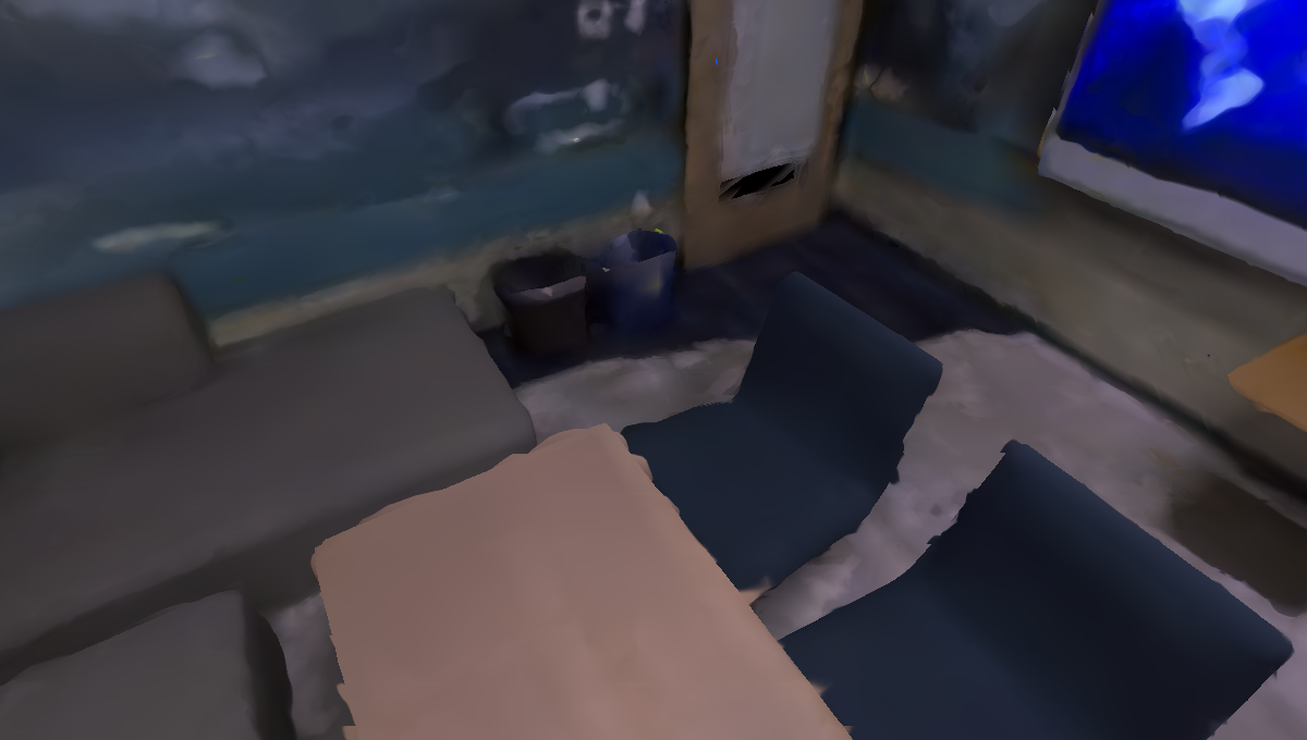
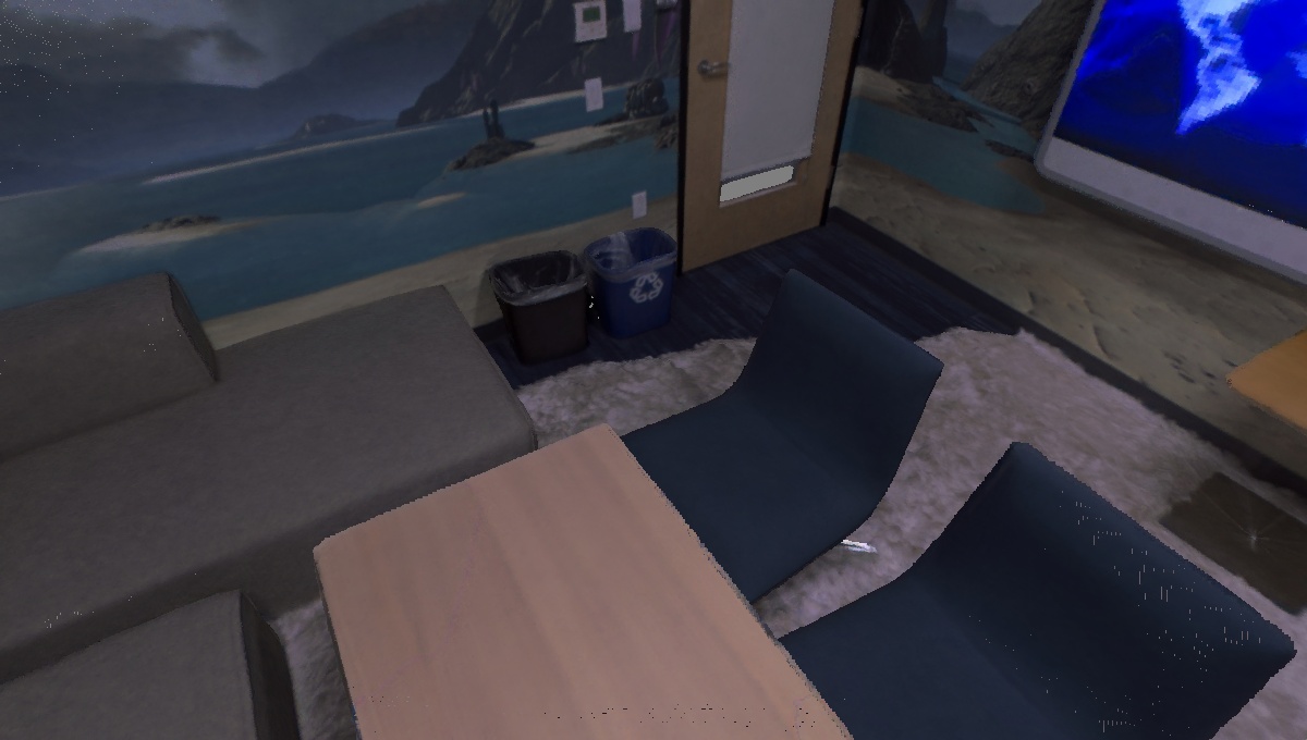
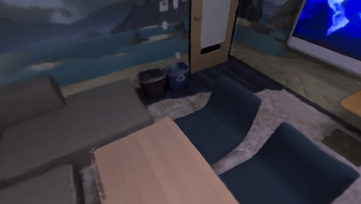
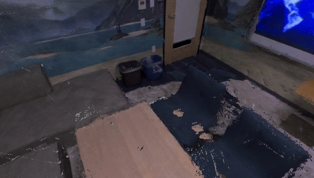
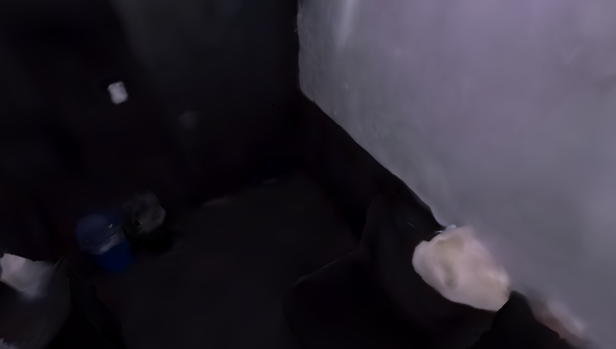
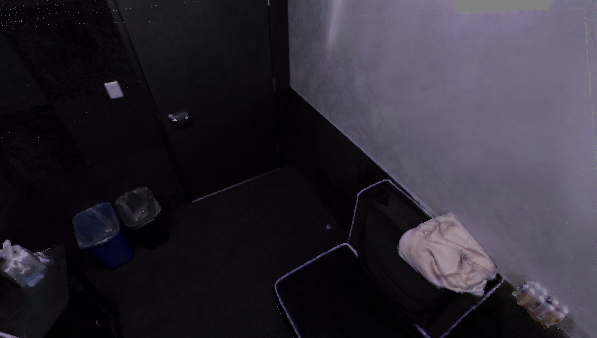
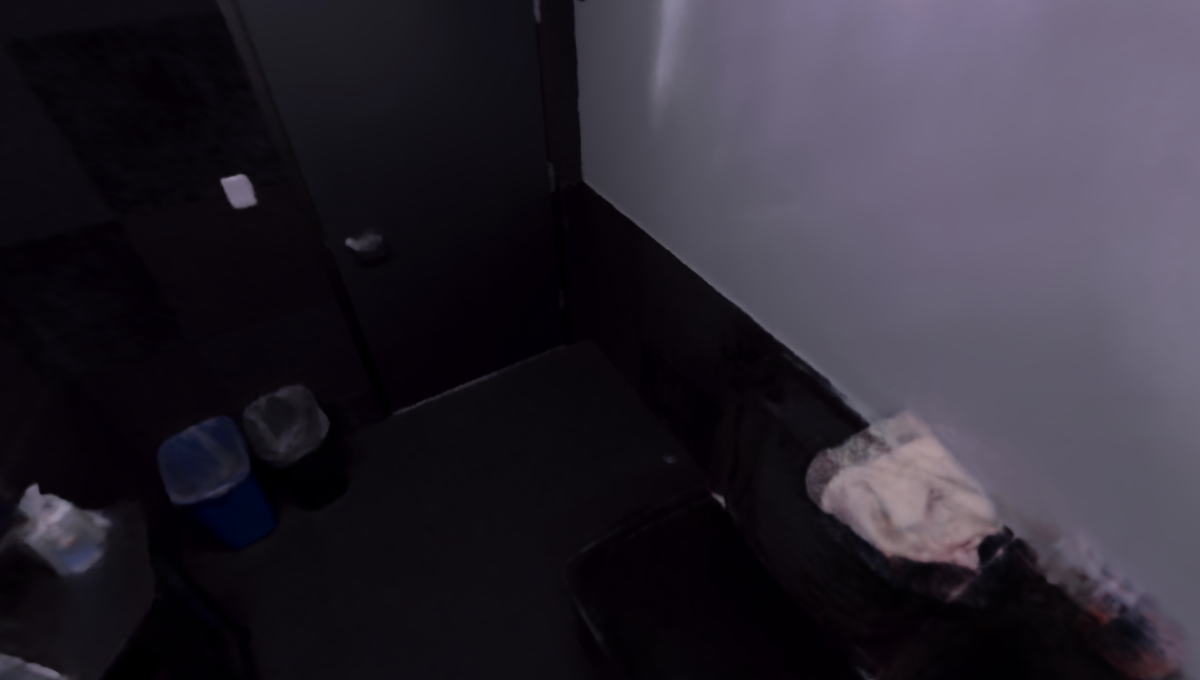
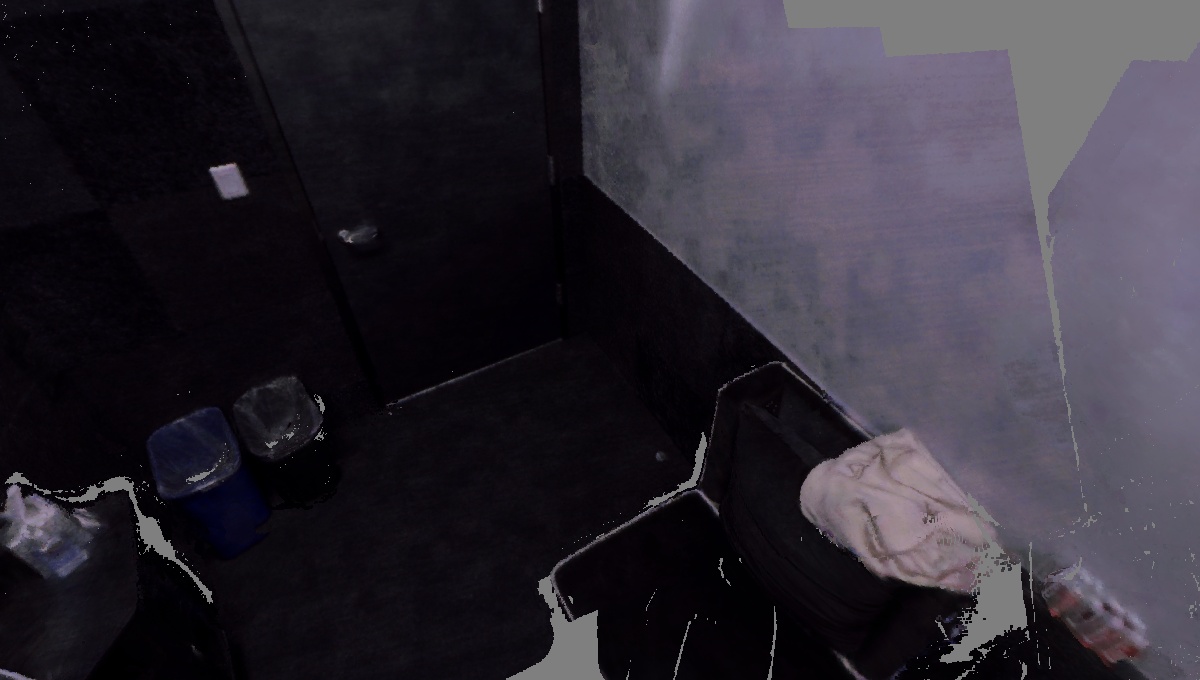
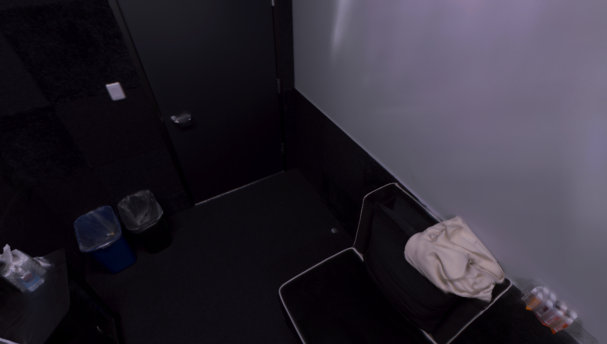
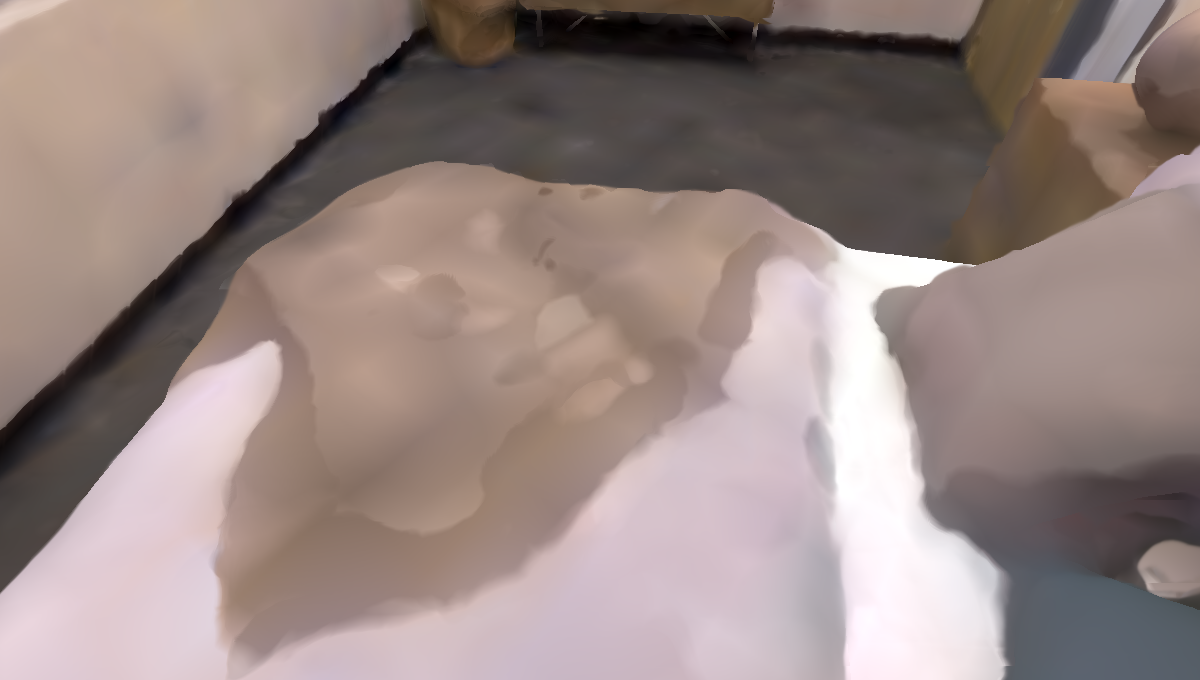
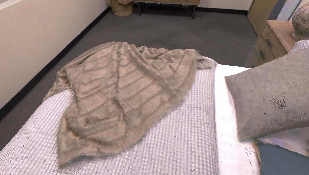
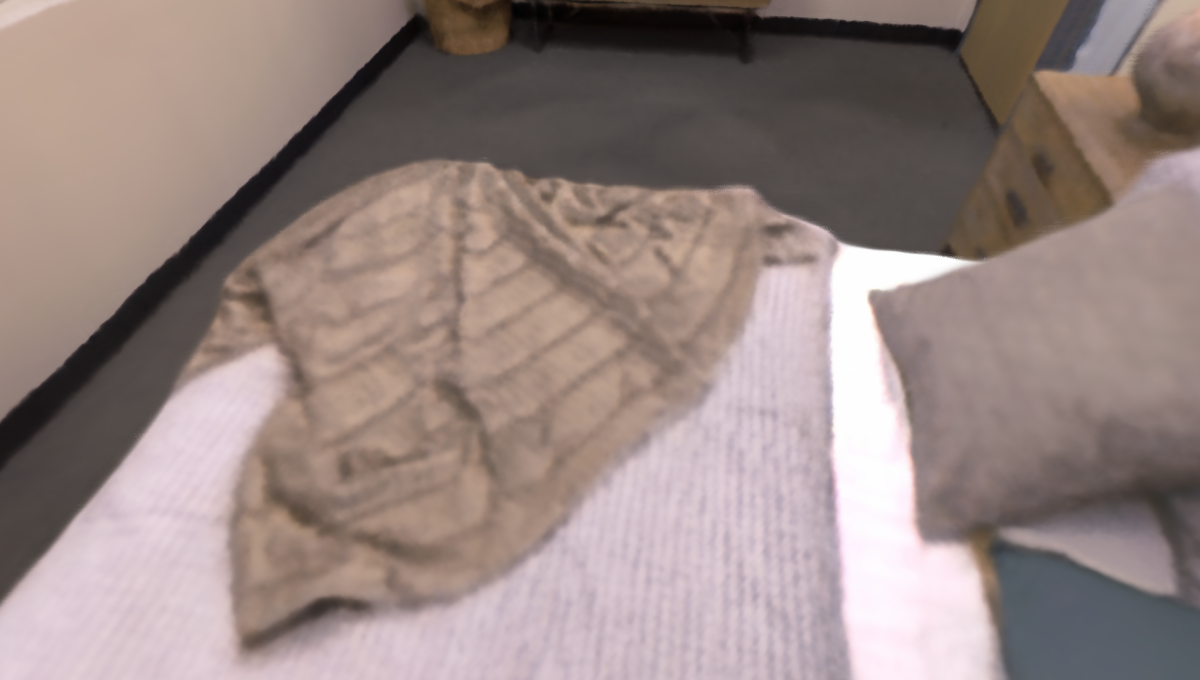
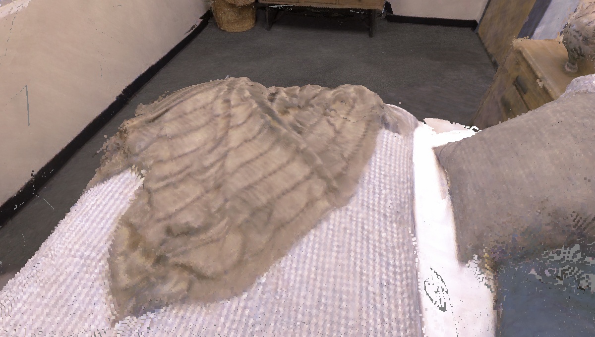
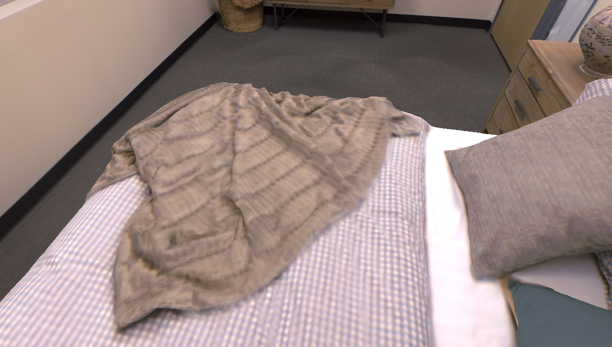
NICE-SLAM	Ours	NICER-SLAM	Ours	GT
RGB-D Input		RGB Input

Figure 16: Qualitative evaluation on replica.

To better illustrate this issue, we test on our own dataset for Dense Mono-SLAM purpose in large scene, with mostly xy-directional motion.

Besides, we find that recent SOTA NeRF-like Dense SLAM, NICER-SLAM, highly focus on the repeated encircling capturing of a object/scene. This is because NICER-SLAM theoretically expires on large scale scene: 1) NICER-SLAM works in bounded model, the poses are required to bound the scene (from their open release); 2) NICER-SLAM’s hashgrid resolution is preset to $2048$ with about 24 GB usage of GPU memory. But this is far too low for a large scene, while it is hard to increase the resolution further. (This is also the reason why the unbounded multi-hashgrid method, NSLF-OL [15], uses SLF instead of NeRF). So when scale increase, NICER-SLAM’s tracking and then mapping will dysfunction. Even new branch, Gaussian Splatting-based Dense Mono SLAM, MonoGS, also rarely test on large scale. While SLAM in robotics are usually excircle-like capturing the scene.

Therefore, to better explore the performance, our dataset mainly contains middle- and large-range scenes which are rarely involved by them.

VI-E Dense Mono-SLAM Purpose dataset

The above tests give an overview of the performance of the tracker and the reconstructor.

We collect this dataset because we find that the current RGB-D sequences are all intended for RGB-D tracking or dense RGB-D reconstruction in small scene. Due to the fact that RGB-D sequences contain real 3D metric depth, the sequence can simply move arbitrarily. For example, in ScanNet and Replica there is a lot of almost purely rotational motion.

On the other hand, monocular sequences dataset are only used for tracking and SfM purposes because no depth ground truth is available. For Dense Mono-SLAM, however, the challenge goes beyond tracking and mapping. Unlike Mono-SLAM that only estimates sparse points with matching pairs, dense Mono-SLAM requires a much larger region to cover.

Moreover, in the real robotics application, the scene is usually captured on large scene and non-repeat capturing which is rarely involved in recent Dense Mono SLAM SOTAs.

Therefore, we have not found any published dataset that is primarily for Dense Mono SLAM purposes in robotics. To fill this gap, we hereby present the first large-scale RGB-D/L dataset for dense mono-SLAM purposes:

• Mid-scale ($\sim 20\times 10m$) scene (RGB-D) as Fig. 17b,

• Large-scale ($\sim 80\times 50m$) scene (RGB-L) as Fig. 17b,

• Small-scale ($\sim 5\times 5m$) scene (RGB) as Fig. 17b,

• Very-large-scale ($\sim 300\times 200m$) scene (RGB-L) as Fig. 17b

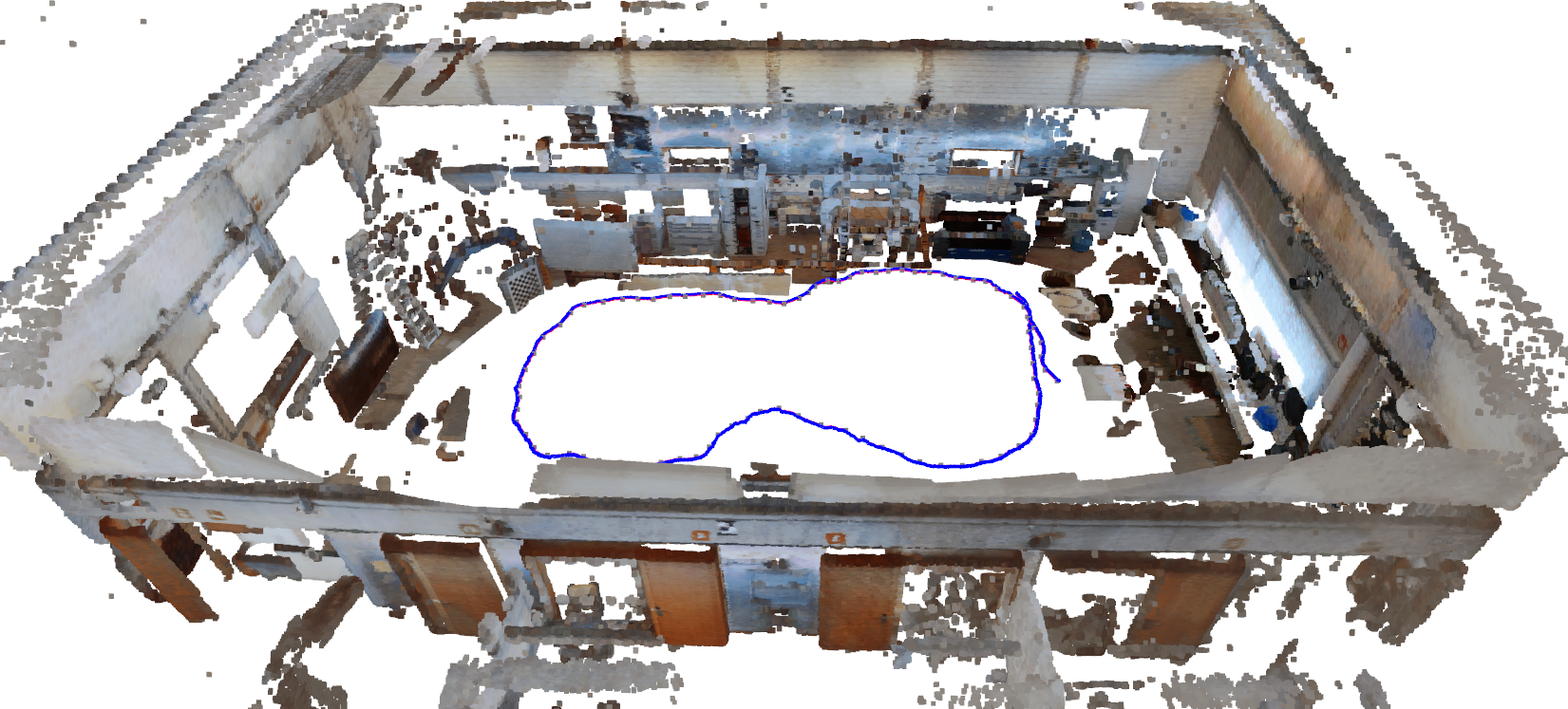
(a) width=.5

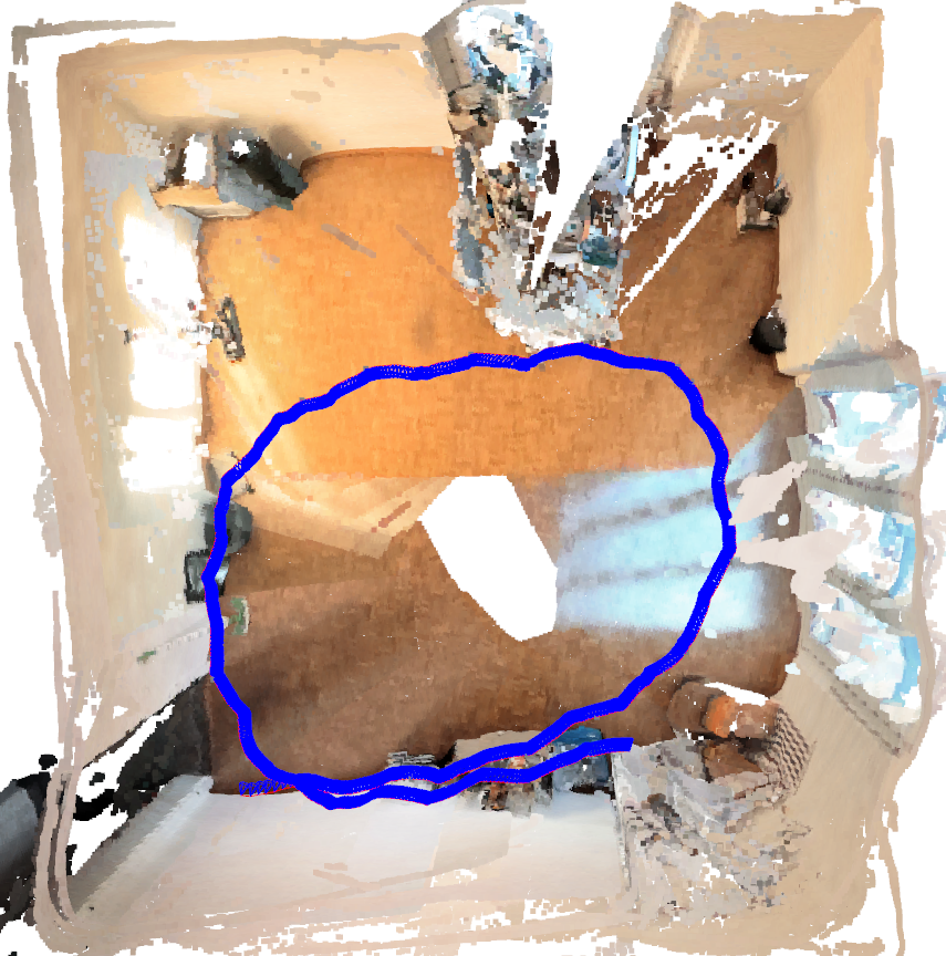
[width=.5][Schloss (RGB-L)]
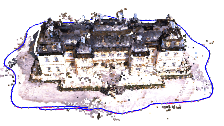
[width=.3][Living room (RGB)] [width=.5][Univ land (RGB-L)]

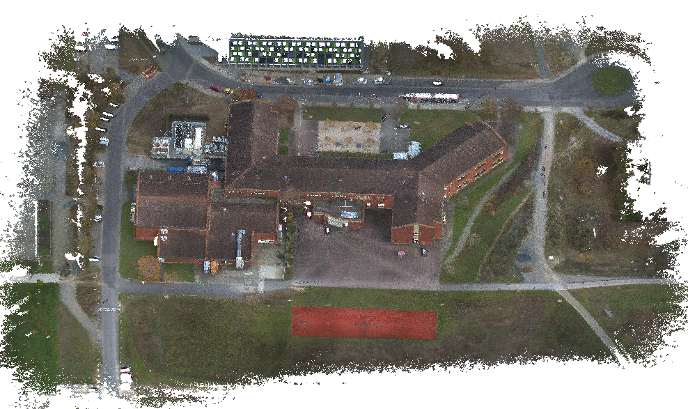
(b) Our dataset with different ranges.

We capture our mid-range data, Robotics Hall, with an Azure Kinect RGB-D camera. Because of the range limitation of Kinect Depth ($1m-5m$), we turn to RGB-L for large-range data, Schloss Veitshöchheim. For small-range data, living room, we use cell phone for just quick quality demonstration. To explore the extreme, we capture very large-range data, university land with an aerial view RGB-L capture.

Figs. 17b, 17b and 17b’s trajectory is a circle because the target are on the same level. Fig. 17b’s drone trajectory is parallel to the ground because the aerial view also well fits the $xy$-directional translation.

In the previous test, we align the surface result with ICP, which becomes challenging in the large scene due to the large partial non-overlap. To standardize the comparison, in our dataset, we use the alignment matrix from trajectory comparison to transform the result reconstruction to ground truth.

VI-E1 Mid-scale data

TABLE VII: Test on robotics hall of our dataset.

NICER. MonoGS Ours Ours (RGB-D) ATE [m] $\downarrow$ 2.44 2.17 0.59 0.22 Acc. [m]$\downarrow$ 1.009 0.724 0.360 0.138 Comp. [m]$\downarrow$ 1.246 0.837 0.368 0.141 Comp. Ratio [%]$\uparrow$ 33.11 49.58 74.84 99.13 PSNR $\uparrow$ 19.20 - 15.13 14.65 SSIM $\uparrow$ 0.690 - 0.442 0.468 LPIPS${}_{alex}$ $\downarrow$ 0.449 - 0.628 0.615 Time 8 hours 25 min. 10 min. 5 min.

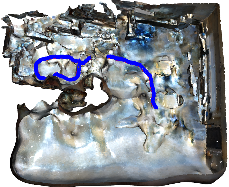
(c) width=.5

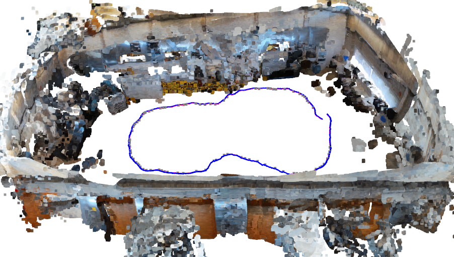
[width=.5][MonoGS]
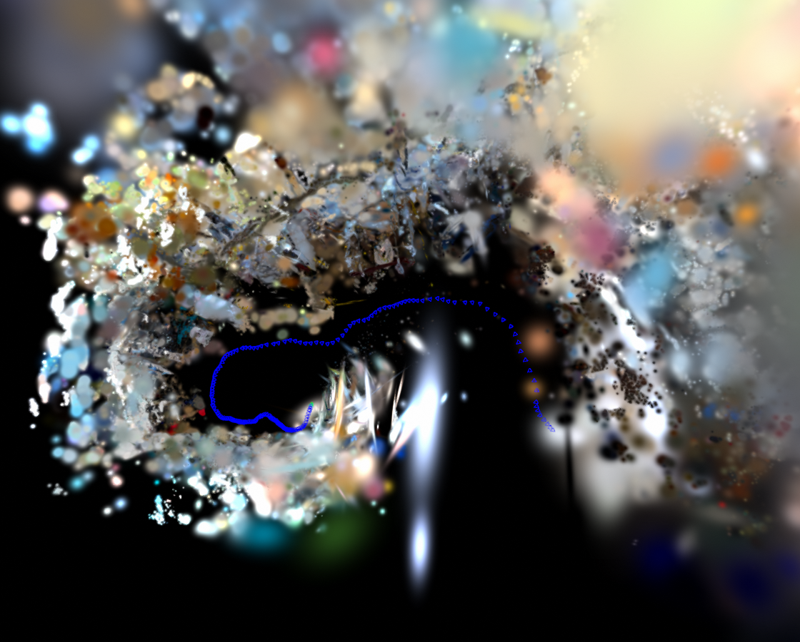
[width=.5][Ours (RGB)] [width=.5][Ours (RGB-D)]

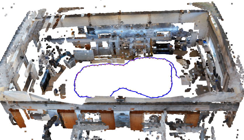
(d) Test result on our mid-range scene. Trajectories are plotted blue.

For a handheld camera, since our task is mainly with scene modeling, our facing direction of the camera is inside-out. Therefore, our capture scheme should follow a certain rule, as shown in Fig. 17b:

• move in circle in the scene

• viewing direction is perpendicular to the moving direction.

Please find Table VII the result on robotics hall. SceneFactory can easily achieve best tracking and reconstruction than two most new Dense Mono SLAM SOTA, NICER-SLAM and MonoGS.

However, we find NICER-SLAM works better on image rendering even with much worse tracking and inconsistent scale. To unfold the truth, we visualize the trajectory with reconstruction. Please find Fig. 18d, both NICER-SLAM and MonoGS severely suffer the scale. This further confirms our speculation: The tight coupled Dense Mono SLAM SOTAs (NICER-SLAM, MonoGS) models attend to one thing and lose sight of another.

Besides, NICER-SLAM’s open release need preprocess of data sequence (COLMAP and more), which takes much more hours than the $8h$ in table. MonoGS is relatively faster, but the result can hardly be viewed in any non-trained view. Which is, you can only view the mid-range and large-range (next test) in the same trained view. As claims in NSLF-OL [15], this is not usable in SLAM because SLAM captures contains very sparse view-directions.

VI-E2 Large-scale data

TABLE VIII: Test on schloss of our dataset.

NICER. MonoGS Ours Ours (RGB-L) ATE [m] $\downarrow$ - 12.90 0.31 0.37 Acc. [m]$\downarrow$ - 7.050 5.074 0.423 Comp. [m]$\downarrow$ - 19.956 0.215 0.321 Comp. Ratio [%]$\uparrow$ - 2.6435 95.67 86.54 Time 4 (28%) hours 2 hours 13 min. 9 min.

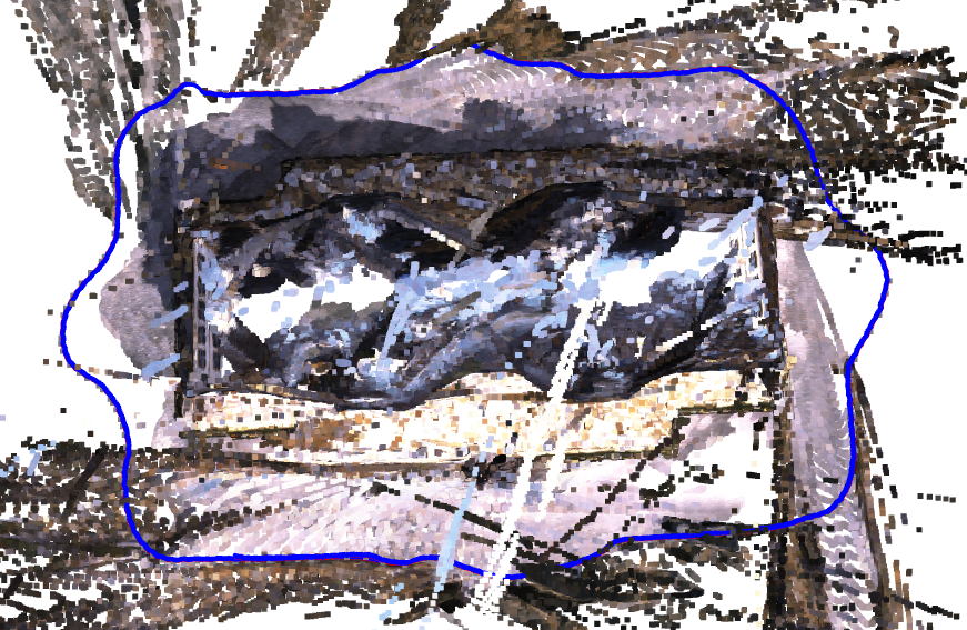
[width=.5][MonoGS]
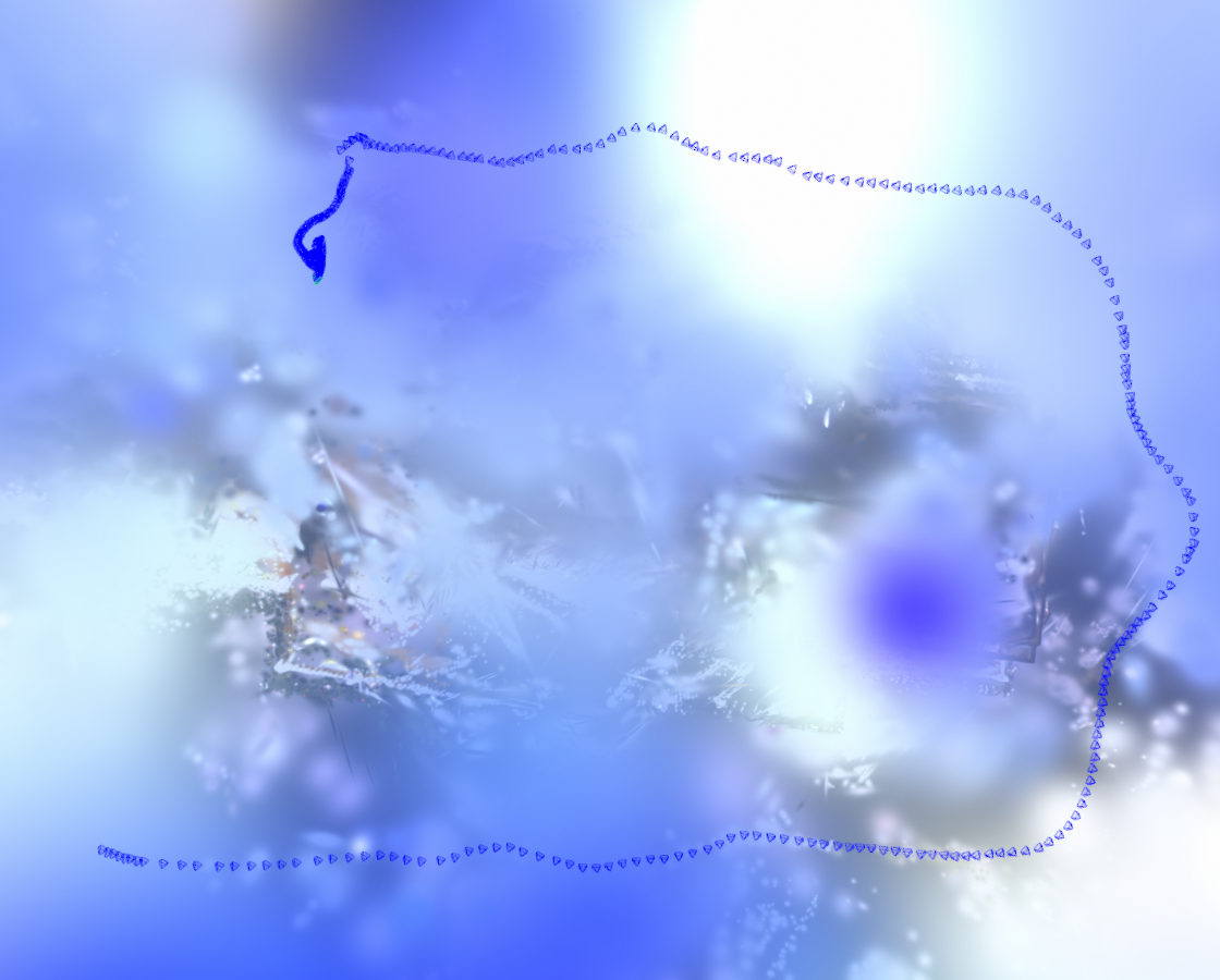
[width=.5][Ours (RGB)] [width=.5][Ours (RGB-L)]

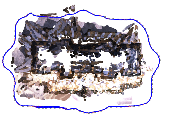
(e) width=.5

(f) Test result on our large-range scene.

For even larger scenes, RGB-D camera dysfunctions, therefore, we turn to Livox LiDAR to provide the metric depth.

We use our handheld RGB-L camera to capture scenes. Because the range is large, our target should be captured outside-in following the same rule as Section VI-E1.

For the larger range scene, from Table VIII, NICER-SLAM fails at $28\%$, MonoGS shows very large tracking error. This can also be revealed by the Fig. 19f, that MonoGS loss the scale in the middle. Besides of the better performance on large-range, the time cost should also be considered. NICER-SLAM takes $4$ hours for only $28\%$ without the counting of preprocessing. MonoGS takes $2$ hours. While ours are still in a acceptable range.

VI-E3 Aerial-view data test

To better demonstrate the potential, we further extend the test scale to very-large. That is too large to capture with basic hand-held devices. Therefore we turn to the aerial devices.

The data is captured with a custom made UAV (DJI Matrice 300 RTK) featuring a LUCID camera and a co-clibrated OUSTER OS1 laser scanner flying over an university bulding, which is a former high-school.

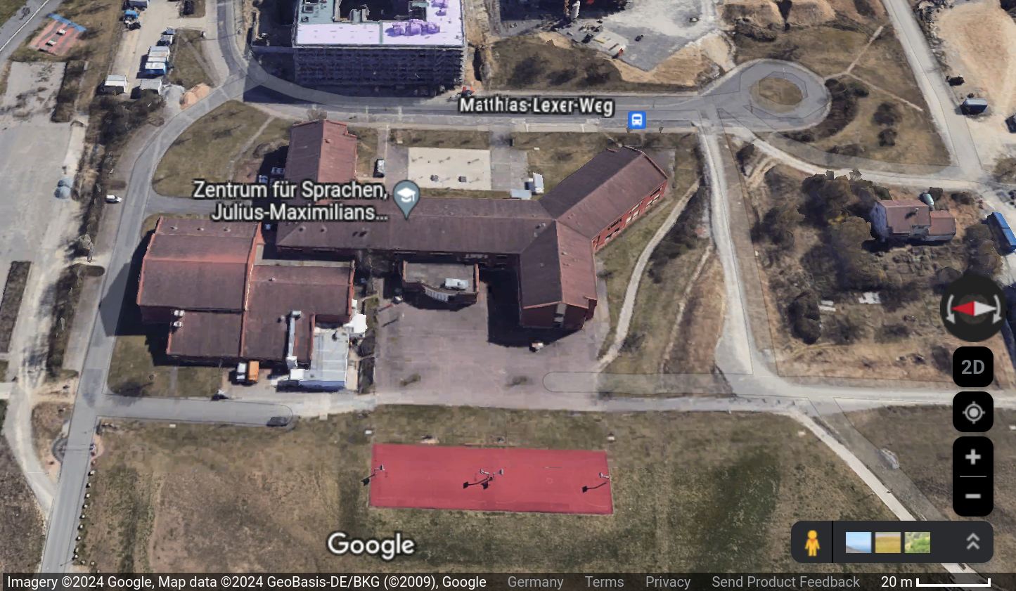
(g) width=.5

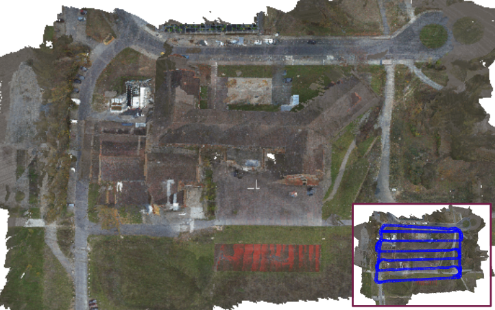
(h) width=.5

Figure 20: SceneFactory’s Dense Mono SLAM on our very-large range scene.

The Dense SLAM result are demonstrated in Fig. 20. Without the use of metric depth. SceneFactory can provide a high quality reconstruction of this very-large scene.

VI-F Exclusive Applications

Besides of previously demonstrated hot tasks, SceneFactory also support more usages.

VI-F1 LiDAR Completion

Our ScaleCov model supports completion of metric LiDAR depth. Given RGB and sparse depth image from Livox, ScaleCov regresses the full depth and variance to the customers. We provide one example in Fig. 21b.

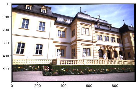
(a) width=.5

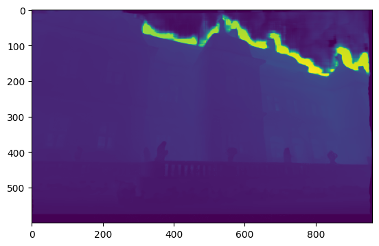
[width=.5][Livox depth]
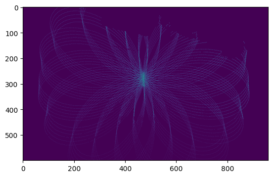
[width=.5][Completed depth] [width=.5][Depth variance]

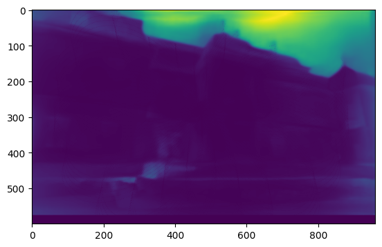
(b) Complete LiDAR depth with ScaleCov.

This technique is also utilized in previous test Fig. 19f.

VI-F2 Dense Depth-only SLAM

Color sensors are usually more sensitive to the surroundings. When color sensor dysfunction (because of poor lighting condition or even night), the depth sensor could instead plays an role.

SceneFactory implement depth-only SLAM under with the factory lines of depth-flexion and RGB-D SLAM. Which is firstly transform depth image to trackable RGB image with depth-flexion. Then the application is employed same as our RGB-D SLAM application.

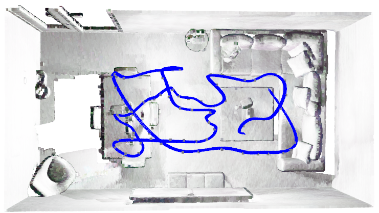
Figure 22: Depth-only SLAM result. (We cut the ceiling for better visualization.)

Please find Fig. 22 our demo of office2 in replica dataset, with only depth as input, The reconstruction result is with high quality and smoothness.

VII Conclusion

In this paper, we have introduced a workflow-centric and unified framework for incremental scene modeling, called SceneFactory. Following the structure of a “Factory”, we have designed “assembly lines” for a wide range of applications, to achieve high flexibility, adaptability and production diversification.

In addition, within the framework, we propose an unposed & uncalibrated multi-view depth estimation model for high flexible use. We introduce surface accessible surface light field design together with improved point rasterization to enable the surface query for the first time.

Our experiments show that SceneFactory is highly competitive or even better than compact SOTAs in such applications. The high quality and broad applicability of the design further enhances the progress of our design.

Needless to say, a lot of work remains to be done. In future work, we will concentrate on adding more applications to the production lines, e.g., deformable reconstruction, active SLAM, or scene understanding [59].

Supplementary

-A Good Neighbor Selection

The dense bundle adjustment relies on the selection of good neighbors. We choose neighbor frames by filtering the relative poses following Algorithm 2.

1 Function FindGoodNeighbors($[\mathbf{G}_{nb,1},\cdots],\mathbf{G}_{i}),\tau_{nb}=2$):

       // select frame by relative pose

2       $ids=[];Ts=[]$

3       for $\mathbf{G}_{j}\in[\mathbf{G}_{nb,1},\cdots]$ do

             // transformation from i to j

4             $\mathbf{T}_{ji}=\mathbf{G}_{i}^{-1}\mathbf{G}_{j};$

5             $\mathbf{R}_{ji},\mathbf{t}_{ji}=\mathbf{T}_{ji};$

6             $l_{baseline}=||\mathbf{t}_{ji}||_{2};$

7             $\theta_{facing}=\arccos([0,0,1]\mathbf{R}_{ji}[0,0,1]^{T});$

8             if $l_{baseline}>\tau_{baseline}$ and $\theta_{facing}>\tau_{facing}$  then

9                   $ids.append(j);$ $Ts.append(\mathbf{T}_{ji})$

10             end if

11            

12       end for

13      if $len(ids)<\tau_{nb}$ then

14             return $\emptyset;$

15      else

             // return the best $\tau_{nb}$ XY directional baselines

16             return $SortByBaselineXY(ids,Ts)[:\tau_{nb}];$

17       end if

18      

19

20

End Function

Algorithm 2 Depth neighbor frame selection.

-B Improved Point Rasterization Ablation Test

Effect of Adaptive Radius

Please find Fig. 23b, there is black hole on the desk. This is because of the fix radius of pytorch3d’s point rasterization in NDC space. Which would be much more severe when camera goes even closer. While our IPR doesnot have this problem.

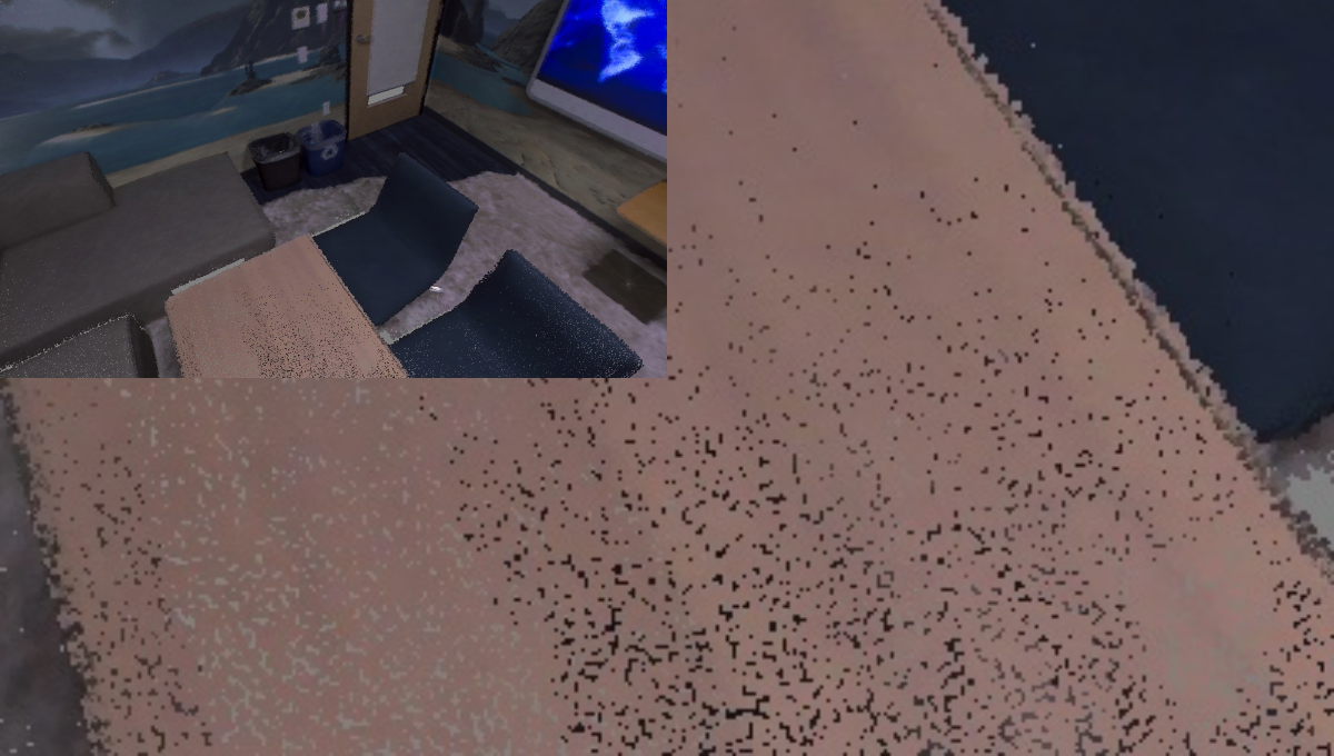
(a) width=.48

[width=.48][Ours Rast. ($\sim 0.025s$)]

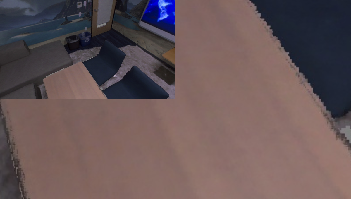
(b) Effect of Adaptive Radius and our implementation in arbitrary view.

Effect of First-layer filter

Besides of the adaptive radius. Our IPR can also get the surface with layer filter as in Fig. 24. Without the layer filter, the result surface points will lay in the middle of multiple surface layers and thus result in a vacancy during color rendering.

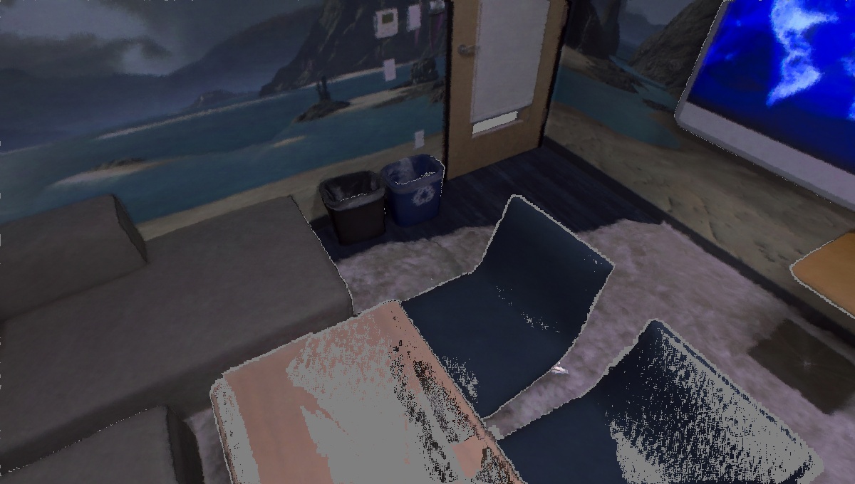
(c) width=.48

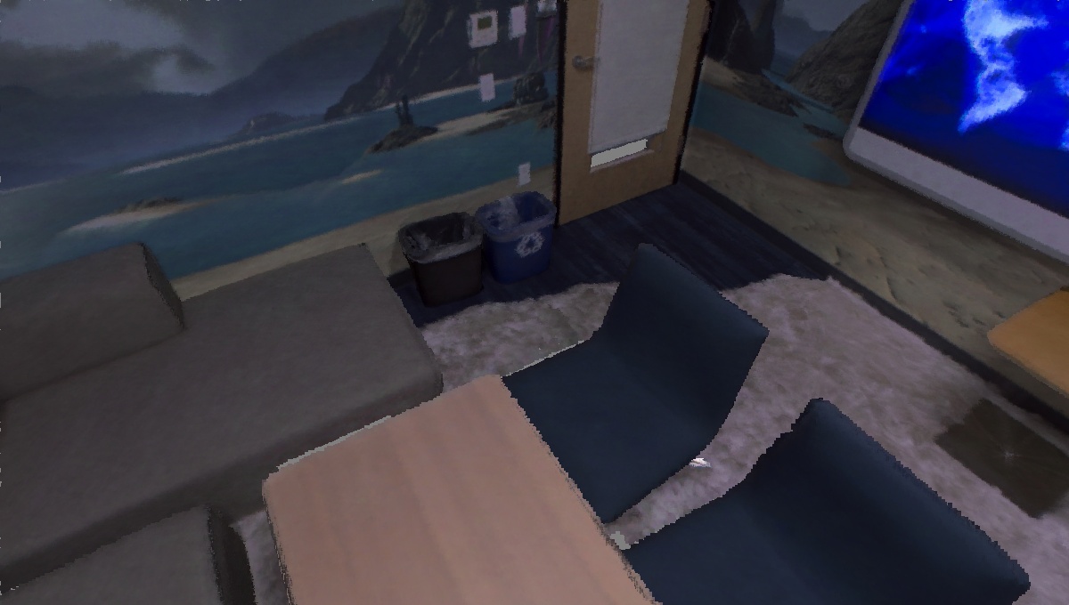
(d) width=.48

Figure 24: Effect of Layer Filter.

-C Description of the Sensor Systems

For collecting our own RGB-X dataset, described in Sec. VI-A2, two commercial sensors are employed: the Microsoft Azure Kinect RGB-D sensor and the built-in camera of a Xiaomi Redmi smartphone. Furthermore, two custom-built sensor systems are used for capturing the datasets:

Handheld mapping system

Our custom-built handheld mapping device is show in Fig. 11(a). It is based on a commercial camera rig with the sensors mounted to the top bar. The sensors are a Livox AVIA Lidar and two IDS U3-30C0CP global-shutter cameras with a Sony IMX392 2.35 MPixel RGB CMOS sensor. The Lidar sensor has a Field of View (FoV) of $70.4^{\circ}\times 77.2^{\circ}$. The cameras are equipped with 4 mm lenses, which results in a similar FoV of $77.3^{\circ}\times 61.9^{\circ}$. Below the sensors a 3D printed enclosure is mounted with an embedded PC for data recording and power supply electronics. Cameras and Lidar are co-calibrated using a calibration board.

From the system we extract a synchronized RGB-L data stream with Lidar scans and camera images with 10 Hz. While the system features stereo cameras, in this work we focus on mono-SLAM. Therefore, only the camera closest to the Lidar sensor is used. The data is captured with the system handheld and an average walking speed of 0.84 $\frac{m}{s}$. During data collection the sensors always points towards the captured object. The trajectory around Veitshöchheim Palace is 251 m long and was captured in 5 min. It consists of 3000 Lidar scans and 3000 RGB images.

UAV mapping system

The UAV mapping system is based on the DJI Matrice 300 RTK and is shown in Fig. 11(b). It carries an Ouster OS1-128 Lidar and a LUCID Vision Labs Phoenix PHX032S-CC global-shutter camera with a Sony IMX265 3.2 MPixel RGB CMOS sensor. The Lidar sensor has a FoV of $360^{\circ}\times 45^{\circ}$. The camera is used with a 4.5 mm fixed lens with a horizontal FoV of $84.7^{\circ}$. The co-calibrated camera is mounted directly on top of the Lidar sensor. For the data collection an embedded PC is mounted on top of the UAV. The aerial imagery is captured with an oblique angle and a lawnmower pattern flight trajectory.

References

- [1] J. Engel, T. Schöps, and D. Cremers, “Lsd-slam: Large-scale direct monocular slam,” in European conference on computer vision. Springer, 2014, pp. 834–849.
- [2] R. Mur-Artal and J. D. Tardós, “Orb-slam2: An open-source slam system for monocular, stereo, and rgb-d cameras,” IEEE transactions on robotics, vol. 33, no. 5, pp. 1255–1262, 2017.
- [3] C. Campos, R. Elvira, J. J. G. Rodríguez, J. M. Montiel, and J. D. Tardós, “Orb-slam3: An accurate open-source library for visual, visual–inertial, and multimap slam,” IEEE Transactions on Robotics, vol. 37, no. 6, pp. 1874–1890, 2021.
- [4] K. Ebadi, L. Bernreiter, H. Biggie, G. Catt, Y. Chang, A. Chatterjee, C. E. Denniston, S.-P. Deschênes, K. Harlow, S. Khattak, L. Nogueira, M. Palieri, P. Petráček, M. Petrlík, A. Reinke, V. Krátký, S. Zhao, A.-a. Agha-mohammadi, K. Alexis, C. Heckman, K. Khosoussi, N. Kottege, B. Morrell, M. Hutter, F. Pauling, F. Pomerleau, M. Saska, S. Scherer, R. Siegwart, J. L. Williams, and L. Carlone, “Present and Future of SLAM in Extreme Environments: The DARPA SubT Challenge,” IEEE Transactions on Robotics, vol. 40, pp. 936–959, 2024.
- [5] C. Kerl, J. Sturm, and D. Cremers, “Dense visual slam for rgb-d cameras,” in 2013 IEEE/RSJ International Conference on Intelligent Robots and Systems. IEEE, 2013, pp. 2100–2106.
- [6] R. A. Newcombe, S. Izadi, O. Hilliges, D. Molyneaux, D. Kim, A. J. Davison, P. Kohi, J. Shotton, S. Hodges, and A. Fitzgibbon, “Kinectfusion: Real-time dense surface mapping and tracking,” in 2011 10th IEEE international symposium on mixed and augmented reality. Ieee, 2011, pp. 127–136.
- [7] M. Bloesch, J. Czarnowski, R. Clark, S. Leutenegger, and A. J. Davison, “Codeslam—learning a compact, optimisable representation for dense visual slam,” in Proceedings of the IEEE conference on computer vision and pattern recognition, 2018, pp. 2560–2568.
- [8] J. Czarnowski, T. Laidlow, R. Clark, and A. J. Davison, “Deepfactors: Real-time probabilistic dense monocular slam,” IEEE Robotics and Automation Letters, vol. 5, no. 2, pp. 721–728, 2020.
- [9] L. Koestler, N. Yang, N. Zeller, and D. Cremers, “Tandem: Tracking and dense mapping in real-time using deep multi-view stereo,” in Conference on Robot Learning. PMLR, 2022, pp. 34–45.
- [10] Z. Teed and J. Deng, “Droid-slam: Deep visual slam for monocular, stereo, and rgb-d cameras,” Advances in neural information processing systems, vol. 34, pp. 16 558–16 569, 2021.
- [11] A. Rosinol, J. J. Leonard, and L. Carlone, “Probabilistic volumetric fusion for dense monocular slam,” in Proceedings of the IEEE/CVF Winter Conference on Applications of Computer Vision, 2023, pp. 3097–3105.
- [12] Z. Yu, S. Peng, M. Niemeyer, T. Sattler, and A. Geiger, “Monosdf: Exploring monocular geometric cues for neural implicit surface reconstruction,” Advances in neural information processing systems, vol. 35, pp. 25 018–25 032, 2022.
- [13] M. M. Johari, C. Carta, and F. Fleuret, “Eslam: Efficient dense slam system based on hybrid representation of signed distance fields,” in Proceedings of the IEEE/CVF Conference on Computer Vision and Pattern Recognition, 2023, pp. 17 408–17 419.
- [14] A. Rosinol, J. J. Leonard, and L. Carlone, “Nerf-slam: Real-time dense monocular slam with neural radiance fields,” arXiv preprint arXiv:2210.13641, 2022.
- [15] Y. Yuan and A. Nüchter, “Online learning of neural surface light fields alongside real-time incremental 3d reconstruction,” IEEE Robotics and Automation Letters, 2023.
- [16] J. Huang, S.-S. Huang, H. Song, and S.-M. Hu, “Di-fusion: Online implicit 3d reconstruction with deep priors,” in Proceedings of the IEEE/CVF Conference on Computer Vision and Pattern Recognition, 2021, pp. 8932–8941.
- [17] N. Ravi, J. Reizenstein, D. Novotny, T. Gordon, W.-Y. Lo, J. Johnson, and G. Gkioxari, “Accelerating 3d deep learning with pytorch3d,” arXiv preprint arXiv:2007.08501, 2020.
- [18] R. A. Newcombe, S. Izadi, O. Hilliges, D. Molyneaux, D. Kim, A. J. Davison, P. Kohi, J. Shotton, S. Hodges, and A. Fitzgibbon, “Kinectfusion: Real-time dense surface mapping and tracking,” in 2011 10th IEEE international symposium on mixed and augmented reality. Ieee, 2011, pp. 127–136.
- [19] W. E. Lorensen and H. E. Cline, “Marching cubes: A high resolution 3d surface construction algorithm,” in Seminal graphics: pioneering efforts that shaped the field, 1998, pp. 347–353.
- [20] Y. Yuan and A. Nüchter, “An algorithm for the se (3)-transformation on neural implicit maps for remapping functions,” IEEE Robotics and Automation Letters, vol. 7, no. 3, pp. 7763–7770, 2022.
- [21] ——, “Uni-fusion: Universal continuous mapping,” IEEE Transactions on Robotics, 2024.
- [22] Z. Zhu, S. Peng, V. Larsson, W. Xu, H. Bao, Z. Cui, M. R. Oswald, and M. Pollefeys, “Nice-slam: Neural implicit scalable encoding for slam,” in Proceedings of the IEEE/CVF Conference on Computer Vision and Pattern Recognition, 2022, pp. 12 786–12 796.
- [23] C.-M. Chung, Y.-C. Tseng, Y.-C. Hsu, X.-Q. Shi, Y.-H. Hua, J.-F. Yeh, W.-C. Chen, Y.-T. Chen, and W. H. Hsu, “Orbeez-slam: A real-time monocular visual slam with orb features and nerf-realized mapping,” in 2023 IEEE International Conference on Robotics and Automation (ICRA). IEEE, 2023, pp. 9400–9406.
- [24] A. Rosinol, J. J. Leonard, and L. Carlone, “Nerf-slam: Real-time dense monocular slam with neural radiance fields,” in 2023 IEEE/RSJ International Conference on Intelligent Robots and Systems (IROS). IEEE, 2023, pp. 3437–3444.
- [25] C. Campos, R. Elvira, J. J. G. Rodríguez, J. M. Montiel, and J. D. Tardós, “Orb-slam3: An accurate open-source library for visual, visual–inertial, and multimap slam,” IEEE Transactions on Robotics, vol. 37, no. 6, pp. 1874–1890, 2021.
- [26] E. Sucar, S. Liu, J. Ortiz, and A. J. Davison, “imap: Implicit mapping and positioning in real-time,” in Proceedings of the IEEE/CVF International Conference on Computer Vision, 2021, pp. 6229–6238.
- [27] T. Müller, A. Evans, C. Schied, and A. Keller, “Instant neural graphics primitives with a multiresolution hash encoding,” ACM transactions on graphics (TOG), vol. 41, no. 4, pp. 1–15, 2022.
- [28] B. Ummenhofer, H. Zhou, J. Uhrig, N. Mayer, E. Ilg, A. Dosovitskiy, and T. Brox, “Demon: Depth and motion network for learning monocular stereo,” in Proceedings of the IEEE conference on computer vision and pattern recognition, 2017, pp. 5038–5047.
- [29] H. Zhou, B. Ummenhofer, and T. Brox, “Deeptam: Deep tracking and mapping,” in Proceedings of the European conference on computer vision (ECCV), 2018, pp. 822–838.
- [30] Z. Teed and J. Deng, “Deepv2d: Video to depth with differentiable structure from motion,” in International Conference on Learning Representations, 2019.
- [31] P. Schröppel, J. Bechtold, A. Amiranashvili, and T. Brox, “A benchmark and a baseline for robust multi-view depth estimation,” in 2022 International Conference on 3D Vision (3DV). IEEE, 2022, pp. 637–645.
- [32] P.-H. Huang, K. Matzen, J. Kopf, N. Ahuja, and J.-B. Huang, “Deepmvs: Learning multi-view stereopsis,” in Proceedings of the IEEE conference on computer vision and pattern recognition, 2018, pp. 2821–2830.
- [33] Y. Yao, Z. Luo, S. Li, T. Fang, and L. Quan, “Mvsnet: Depth inference for unstructured multi-view stereo,” in Proceedings of the European conference on computer vision (ECCV), 2018, pp. 767–783.
- [34] Y. Yao, Z. Luo, S. Li, T. Shen, T. Fang, and L. Quan, “Recurrent mvsnet for high-resolution multi-view stereo depth inference,” in Proceedings of the IEEE/CVF conference on computer vision and pattern recognition, 2019, pp. 5525–5534.
- [35] J. Yang, W. Mao, J. M. Alvarez, and M. Liu, “Cost volume pyramid based depth inference for multi-view stereo,” in Proceedings of the IEEE/CVF conference on computer vision and pattern recognition, 2020, pp. 4877–4886.
- [36] X. Gu, Z. Fan, S. Zhu, Z. Dai, F. Tan, and P. Tan, “Cascade cost volume for high-resolution multi-view stereo and stereo matching,” in Proceedings of the IEEE/CVF conference on computer vision and pattern recognition, 2020, pp. 2495–2504.
- [37] J. Zhang, S. Li, Z. Luo, T. Fang, and Y. Yao, “Vis-mvsnet: Visibility-aware multi-view stereo network,” International Journal of Computer Vision, vol. 131, no. 1, pp. 199–214, 2023.
- [38] E. Brachmann, A. Krull, S. Nowozin, J. Shotton, F. Michel, S. Gumhold, and C. Rother, “Dsac-differentiable ransac for camera localization,” in Proceedings of the IEEE conference on computer vision and pattern recognition, 2017, pp. 6684–6692.
- [39] J. Revaud, Y. Cabon, R. Brégier, J. Lee, and P. Weinzaepfel, “Sacreg: Scene-agnostic coordinate regression for visual localization,” arXiv preprint arXiv:2307.11702, 2023.
- [40] C.-H. Lin, C. Kong, and S. Lucey, “Learning efficient point cloud generation for dense 3d object reconstruction,” in proceedings of the AAAI Conference on Artificial Intelligence, vol. 32, no. 1, 2018.
- [41] J. Wang, B. Sun, and Y. Lu, “Mvpnet: Multi-view point regression networks for 3d object reconstruction from a single image,” in Proceedings of the AAAI Conference on Artificial Intelligence, vol. 33, no. 01, 2019, pp. 8949–8956.
- [42] S. Wang, V. Leroy, Y. Cabon, B. Chidlovskii, and J. Revaud, “Dust3r: Geometric 3d vision made easy,” arXiv preprint arXiv:2312.14132, 2023.
- [43] J. Edstedt, I. Athanasiadis, M. Wadenbäck, and M. Felsberg, “Dkm: Dense kernelized feature matching for geometry estimation,” in Proceedings of the IEEE/CVF Conference on Computer Vision and Pattern Recognition, 2023, pp. 17 765–17 775.
- [44] A. Hagemann, M. Knorr, and C. Stiller, “Deep geometry-aware camera self-calibration from video,” in Proceedings of the IEEE/CVF International Conference on Computer Vision, 2023, pp. 3438–3448.
- [45] M. Hu, W. Yin, C. Zhang, Z. Cai, X. Long, H. Chen, K. Wang, G. Yu, C. Shen, and S. Shen, “A versatile monocular geometric foundation model for zero-shot metric depth and surface normal estimation,” 2024.
- [46] W. Yin, C. Zhang, H. Chen, Z. Cai, G. Yu, K. Wang, X. Chen, and C. Shen, “Metric3d: Towards zero-shot metric 3d prediction from a single image,” in Proceedings of the IEEE/CVF International Conference on Computer Vision, 2023, pp. 9043–9053.
- [47] E. Dexheimer and A. J. Davison, “Learning a depth covariance function,” in Proceedings of the IEEE/CVF Conference on Computer Vision and Pattern Recognition, 2023, pp. 13 122–13 131.
- [48] Z. Teed, L. Lipson, and J. Deng, “Deep patch visual odometry,” Advances in Neural Information Processing Systems, vol. 36, 2024.
- [49] R. Lösch, M. Sastuba, J. Toth, and B. Jung, “Converting depth images and point clouds for feature-based pose estimation,” in 2023 IEEE/RSJ International Conference on Intelligent Robots and Systems (IROS), 2023.
- [50] A. Dai, A. X. Chang, M. Savva, M. Halber, T. Funkhouser, and M. Nießner, “Scannet: Richly-annotated 3d reconstructions of indoor scenes,” in Proceedings of the IEEE conference on computer vision and pattern recognition, 2017, pp. 5828–5839.
- [51] A. Geiger, P. Lenz, C. Stiller, and R. Urtasun, “Vision meets robotics: The kitti dataset,” International Journal of Robotics Research (IJRR), 2013.
- [52] T. Schops, J. L. Schonberger, S. Galliani, T. Sattler, K. Schindler, M. Pollefeys, and A. Geiger, “A multi-view stereo benchmark with high-resolution images and multi-camera videos,” in Proceedings of the IEEE conference on computer vision and pattern recognition, 2017, pp. 3260–3269.
- [53] R. Jensen, A. Dahl, G. Vogiatzis, E. Tola, and H. Aanæs, “Large scale multi-view stereopsis evaluation,” in Proceedings of the IEEE conference on computer vision and pattern recognition, 2014, pp. 406–413.
- [54] A. Knapitsch, J. Park, Q.-Y. Zhou, and V. Koltun, “Tanks and temples: Benchmarking large-scale scene reconstruction,” ACM Transactions on Graphics, vol. 36, no. 4, 2017.
- [55] J. L. Schonberger and J.-M. Frahm, “Structure-from-motion revisited,” in Proceedings of the IEEE conference on computer vision and pattern recognition, 2016, pp. 4104–4113.
- [56] J. L. Schönberger, E. Zheng, J.-M. Frahm, and M. Pollefeys, “Pixelwise view selection for unstructured multi-view stereo,” in Computer Vision–ECCV 2016: 14th European Conference, Amsterdam, The Netherlands, October 11-14, 2016, Proceedings, Part III 14. Springer, 2016, pp. 501–518.
- [57] Z. Yang, Z. Ren, Q. Shan, and Q. Huang, “Mvs2d: Efficient multi-view stereo via attention-driven 2d convolutions,” in Proceedings of the IEEE/CVF conference on computer vision and pattern recognition, 2022, pp. 8574–8584.
- [58] R. from http://www.cloudcompare.org/, “Cloudcompare (version 2.11),” 2024.
- [59] Y. Ming, X. Yang, W. Wang, Z. Chen, J. Feng, Y. Xing, and G. Zhang, “Benchmarking neural radiance fields for autonomous robots: An overview,” arXiv preprint arXiv:2405.05526, 2024.