Adaptive Exploration for Data-Efficient General Value Function Evaluations
Abstract
General Value Functions (GVFs) (Sutton et al, 2011) are an established way to represent predictive knowledge in reinforcement learning. Each GVF computes the expected return for a given policy, based on a unique pseudo-reward. Multiple GVFs can be estimated in parallel using off-policy learning from a single stream of data, often sourced from a fixed behavior policy or pre-collected dataset. This leaves an open question: how can behavior policy be chosen for data-efficient GVF learning? To address this gap, we propose GVFExplorer, which aims at learning a behavior policy that efficiently gathers data for evaluating multiple GVFs in parallel. This behavior policy selects actions in proportion to the total variance in the return across all GVFs, reducing the number of environmental interactions. To enable accurate variance estimation, we use a recently proposed temporal-difference-style variance estimator. We prove that each behavior policy update reduces the mean squared error in the summed predictions over all GVFs. We empirically demonstrate our method’s performance in both tabular representations and nonlinear function approximation.
1 Introduction
The ability to predict many different signals is a key attribute of human, animal, and likely artificial intelligence too. In reinforcement learning (RL), a model of predictive knowledge that is grounded in an agent’s sensory experience is formulated as General Value Functions (GVFs) (Sutton et al., 2011). Each GVF is defined by a unique policy and pseudo-reward known as cumulant. GVFs generalize the classic concept of a value function. They measure an agent’s expected cumulative discounted value of cumulant, where the discount factor may vary as a function of state (instead of being fixed). A significant subclass of GVFs focus on predicting these values for a given fixed policy. These predictive GVFs can answer questions like: “How much time is there before the agent hits a wall, given its current way of moving?” or “What is the probability of the agent to collect a particular object in an allotted time, under a given policy” (White et al., 2015; Schlegel et al., 2021; Sherstan, 2020).
As each GVF may be defined in terms of a unique policy-cumulant pair, this requires off-policy learning to update all GVFs in parallel. Prior works have estimated GVF values by either using a pre-collected datasets (Xu et al., 2022) or by following a fixed, randomized behavior policy (Sutton et al., 2011). However, these methods can suffer from large value estimation errors if the behavior policy or dataset is ill-suited for learning a particular GVF. Here, “ill-suited” means that the behavior policy can be very different from the GVF policies or the behavior policy does not sufficiently visit regions crucial for learning GVFs. Our work addresses this gap by focusing on the question of exploration for evaluating GVFs: how can we adapt an agent’s behavior policy to strategically sample data for multiple GVF evaluations in parallel? While exploration has been extensively studied in context of optimal control in Markov Decision Processes (MDP), the question of constructing a policy that can learn multiple quantities in parallel has remained largely untouched.
To accurately evaluate multiple GVFs in parallel, we aim to design a behavior policy that minimizes the overall mean squared error (MSE) in their predictions. An intuitive approach would be to follow each GVF’s target policy for some period of time (e.g. one episode) in a round-robin manner, and parallely update all GVFs off-policy. However, this approach can be highly data inefficient as actions are sampled according to given policies, overlooking high-variability regions crucial for learning. To overcome this limitation, we introduce an approach, GVFExplorer, that strategically directs the behavior policy to sample actions in proportion to the total variance across GVF predictions. This strategy is based on the understanding that prioritizing high-variance regions leads to more informative samples which ultimately enhance the accuracy of GVF evaluations. We use an existing temporal difference (TD) based variance estimator (Jain et al., 2021) to allow bootstrapping and iterative updates.
Contributions:
(1) We design an adaptive behavior policy that enables learning multiple GVF predictions accurately and efficiently in parallel [Algorithm 1]. (2) We derive an iterative behavior update rule that directly minimizes the overall prediction error [Theorem 5.1]. (3) We prove that in the tabular setting, each update to the behavior policy reduces the total MSE across GVFs [Theorem 5.2]. (4) We establish the existence of a variance operator that enables us to use TD-based variance estimation [Lemma 6.1]. (5) We empirically demonstrate that GVFExplorer lowers the total MSE when estimating multiple GVFs compared to baseline approaches and enables evaluating a larger number of GVFs in parallel.
2 Related Work
In RL, the exploration literature has mainly focused on exploration for improving policy performance for a single objective (Oudeyer et al., 2007; Schmidhuber, 2010; Jaderberg et al., 2016; Machado et al., 2017; Eysenbach et al., 2018; Burda et al., 2018; Guo et al., 2022). Refer to Ladosz et al. (2022) for a detailed survey on exploration techniques in RL. While related to exploration, our work instead focuses on learning a behavior policy for evaluating multiple GVFs.
Our work is most closely related to other works on learning multiple GVFs. While Xu et al. (2022) studies a similar problem of evaluating multiple GVFs using an offline dataset, our method operates online without any pre-collected samples. Thus, our work avoids the data coverage limitations of offline approaches. Linke et al. (2020) develops exploration for learning GVFs in a stateless bandit context, which does not deal with the off-policy learning or function approximation challenges present in the full Markov Decision Process (MDP) context. Prior works like Hanna et al. (2017) learned a behavior policy for a single policy evaluation problem using a REINFORCE-style (Williams, 1992) variance-based method called BPS. This idea is similar to variance reduction techniques in Monte Carlo Simulation, which use Importance Sampling and derive a minimum-variance sampling strategy (Owen, 2013; Frank et al., 2008). Metelli et al. (2023) also extends this idea to the control setting. However, these methods are focused on single-task evaluation or control. Predicting multiple values is more challenging due to the need to carefully balance action selection among various interrelated learning problems. Perhaps the closest to our work is the algorithm of McLeod et al. (2021), which uses weight changes in the Successor Representation (SR) (Dayan, 1993) as an intrinsic reward to learn a behavior policy that supports multiple predictive tasks. GVFExplorer is simpler, optimizing the behavior policy to directly minimize total prediction error over GVFs, resulting in an intuitive variance-proportional sampling strategy. We will compare the two approaches empirically as well.
3 Preliminaries
Consider an agent interacting with the environment to obtain estimate different General Value Function (GVF) (Sutton et al., 2011). We assume an episodic, discounted Markov decision process (MDP) where is the set of states, is the action set, is the transition probability function, is the -dimensional probability simplex, and is the discount factor.
Each GVF is conditioned on a fixed policy , and has a cumulant . For simplicity, we assume that all cumulants are scalar, and that the GVFs share the environment discount factor . This eases the exposition, but our results can be extended to general multidimensional cumulants and state dependent discount factor .
Each GVF is a value function where . Each GVF can be viewed as answering the question, “what is the expected discounted sum of received while following ?” We can also define action-value GVFs: . Similar to traditional value functions, we have: .
At every time step , the agent is in state , takes an action and receives cumulant values for all , transitioning to a new state . This repeats until reaching a terminal state or a maximum step count. Then the agent resets to a new initial state and starts again. The agent interacts with environment using some behavior policy, . The goal of the agent is to compute the approximate values corresponding to the true GVFs value . We formalize this objective as minimizing the Mean Squared Error (MSE) under some state weighting for all GVFs:
| (1) |
In our experiments, we use the uniform distribution for . In principle, this objective could be generalized to prioritize certain GVFs by using a weighted MSE.
Importance Sampling.
To estimate multiple GVFs with distinct target policies in parallel, off-policy learning is essential. Importance sampling (IS) is one of the primary tools for off-policy value learning (Hesterberg, 1988; Precup, 2000; Rubinstein & Kroese, 2016). IS allows to estimate the expected return under a target policy , using trajectories from a different behavior policy . The probability of trajectory occurring under is denoted by , and under by . The true value for any state can be estimated by sampling actions under as . This IS estimate is unbiased, i.e. . There are also variations of IS that provides lower variance, such as per-decision IS, weighted IS and discounted stationary distribution IS (Precup, 2000).
4 Problem Formulation
As described in the previous section, the goal of the agent is to minimize the total mean squared error (MSE) across the given GVFs (Equation 1). Note that . As we will be using unbiased IS estimation for off-policy correction, the task of reducing the total MSE essentially becomes minimizing the total variance across GVFs. Thus, the crux of our problem is to find a behavior policy that gathers data in such a way as to minimize the variance across the set of GVFs.
Prior works (Kahn & Marshall, 1953; Owen, 2013) have studied a simpler version of the above problem, seeking an optimal behavior policy for estimating a single target policy value using IS through variance reduction:
However, this analytical solution of is infeasible for estimating multiple GVFs due to its dependence on the unknown quantity . To address this limitation and estimate multiple GVFs as well, our approach involves optimizing to minimize the total variance in cumulants across all GVFs, under state weighting :
| (2) |
4.1 Objective Function
To solve this optimization problem, we will rely on the variance function , which measures the variance in the return of target policy in a state when actions are sampled under a different behavior policy . In-depth insights into the variance operator is explored in Section 6. The variance function for a given state is defined as:
Similarly, for each state-action pair, we can define:
In this work, the objective is to find an optimal behavior policy that efficiently collects data to minimize the sum of variances under some desired state distribution . Thus, the objective is:
| (3) |
Next, we present an iterative update for the behavior policy obtained by solving the objective in Equation 3.
5 Theoretical Framework
Theorem 5.1.
(Behavior Policy Update:) Given target policies for , let denote the number of updates to the behavior policy and let be the per-step IS weight. Using the variance state-action function , the behavior policy updates as follows:
| (4) |
Proof.
The proof is presented in Appendix A. ∎
Theorem 5.1 outlined above provides an iterative solution using the variance under the previous behavior policy to guide the next policy . These updates drive the behavior policy to explore areas with higher variability, leading to a decrease in the overall variance and, hence, MSE. Furthermore, this approach of reducing overall variance also allows accurate learning of multiple GVF values with fewer data samples, thereby reducing the number of environmental interactions needed to obtain good approximations. In the next theorem, we will establish that each update from to decrease the overall variance across GVFs, providing monotonic progress towards the overall objective in an oscillation-free manner.
Theorem 5.2.
(Behavior Policy Improvement:) The behavior policy update in Eq.(4) ensures that the aggregated variances across all target policies decrease with each update step , that is,
Proof.
The proof is in Appendix A. ∎
6 Variance Function
The theorems given in the previous section suggest an approach to learn an optimal behavior policy is dependent on the variance function . We will study this variance function in detail now.
What is the Variance Function ?
In an off-policy context, Jain et al. (2021) introduced the variance function , which estimates the variance in return under a target policy using data from a different behavior policy . We will directly use this function as our variance estimator and present it here for completeness. The function for a state-action pair under , with an importance sampling correction factor , is defined as:
| (5) | ||||
Here, is the return at time , and (Sutton & Barto, 2018) is the TD error. The variance function relates the variance under from the current state-action pair to the next, when trajectories are sampled from . This allows us to effectively bootstrap and iteratively update using temporal difference (TD) style method. Similarly, variance given state:
| (6) |
Both state and state-action variances are interconnected, with . Note that the value function is required to compute the TD error . Following Jain et al. (2021), we substitute the value estimate for the true function to compute in Eq.(5) and Eq.(6).
Next, we prove the existence of , which was not actually covered in Jain et al. (2021). This existence proof inherently establishes an upper bound on the IS ratio . This condition limits the divergence of the behavior policy from the target policy, aligning with methodologies like TRPO (Schulman et al., 2015) and Retrace (Munos et al., 2016), which control the stability of policy updates by regulating the divergence.
When does the Variance Function Exists?
Let denote the pseudo-reward and represent the transition probability matrix . The matrix form of is:
| (7) |
The existence of hinges on the invertibility of matrix . Lemma 6.1 establishes the existence of the above inverse using Definitions A.1, A.2 and A.3.
Lemma 6.1.
(Variance Function Existence:) Given a discount factor , the existence of variance function depends on the invertibility of matrix if the below condition is satisfied:
Proof.
Proof in Appendix A. ∎
Lemma 6.1 results in a loose upper bound on the IS weight . This constraint emerges naturally as a necessary condition for the existence of the variance operator in Equation 7.
7 Algorithm
We are now ready to discuss the GVFExplorer algorithm, detailed in Algorithm 1. Our approach uses two networks: one for the value function () and another for the variance function (), each with heads (one head for each GVF). The agent begins with a randomly initialized behavior policy. At each step, the agent observes cumulants for each of the GVFs, then it updates the -network using off-policy TD. In our experiments, we use Expected Sarsa (Sutton & Barto, 2018), which has lower variance than other off-policy learning methods. This happens because Expected Sarsa updates the target with the expected value over the target policy’s actions for the next state value. The TD-error generated by the -network is then used to update the variance network (see Equation 5). We use Expected Sarsa for the -network update as well. The behavior policy is then updated based on the new variance estimates, using Equation 4. This iterative process continues through environment steps, ultimately producing a refined -network for GVF value predictions.
To further enhance the algorithm’s adaptability and efficiency, we incorporate established Deep RL techniques such as Experience Replay Buffer for data reuse and target networks for both and to improve learning stability.
8 Experiments
We investigate the empirical utility of our proposed algorithm in both discrete and continuous state environments. Our experiments are designed to answer the following questions: (a) can GVFExplorer evaluate multiple GVFs efficiently? (b) how does GVFExplorer compare with the different baselines (explained below) in terms of convergence speed and estimation quality? (c) can GVFExplorer handle a large number of GVFs? (d) can GVFExplorer work with non-linear function approximations? The code is available at Github https://github.com/arushijain94/ExplorationofGVFs.
Baselines.
We benchmark GVFExplorer against several different baselines: (1) RoundRobin: uses a round-robin strategy to episodically sample from all target policies and uses off-policy Expected Sarsa for parallel estimation of multiple GVFs; (2) MixturePolicy: similar to RoundRobin, but uses a combined policy from all the given target policies; (3) SR: a Successor Representation (SR) based method which uses a intrinsic reward of total change in SR and reward weights to learn a behavior policy, as in(McLeod et al., 2021). (4) BPS: behavior policy search method originally designed for single target policy evaluation using a REINFORCE-style variance estimator (Hanna et al., 2017); we adapted it by averaging the variance across multiple GVFs (as in our objective). BPS results are limited to tabular settings due to scalability and performance issues. (5) UniformPolicy: a uniform sampling policy over the action space. We include all the relevant hyperparameters and implementation details in Section B.1.
Experimental Settings.
To answer the questions presented above, we consider different settings: (Setting 1): In a tabular setting, we examine two GVFs with distinct target policies but identical cumulants, . (Setting 2): In the same environment, we assess two GVFs with different target policy-cumulant pairs, . (Setting 3): To verify the scalability of proposed method with high number of GVFs, we evaluate combinations of different target policies with different cumulants , resulting in 40 GVFs. (Setting 4): In a continuous state environment with non-linear function approximator, we evaluate two distinct GVFs, . Across these varied settings, we measure the MSE as a function of the the number of actions taken by the agent.
8.1 Tabular Experiments
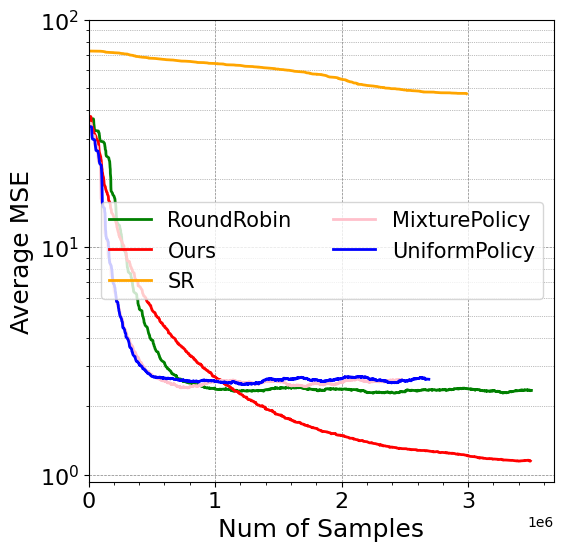
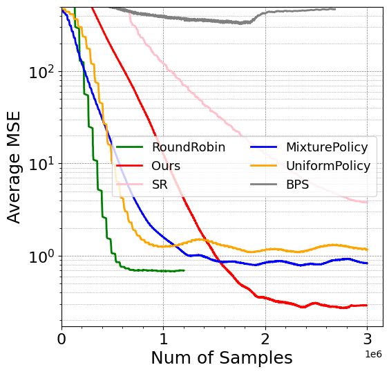
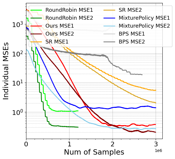
We consider a grid with discrete states and four actions which moves the agent in four cardinal directions. The discount factor is . The environment is stochastic, where with probability, agent uniformly moves in any direction. In (Setting 1), the cumulant is placed at the top left corner with a reward of and zero everywhere else. The agent starts from any non-goal state. The episode terminates either after steps or upon reaching the goal. Detailed description of the two target policies is provided in Section B.1. The true value function is calculated analytically as for MSE computation. Figure 1 compares the averaged MSEs and the individual MSE for the estimated for all algorithms. The results indicate that GVFExplorer reduces the MSE faster, indicating more precise value estimation given the same number of agent-environment interactions.
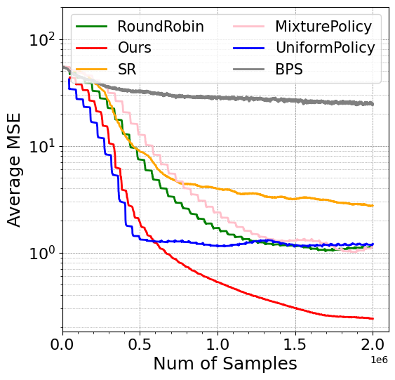
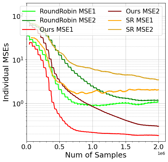
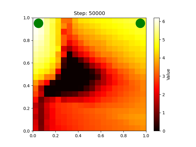
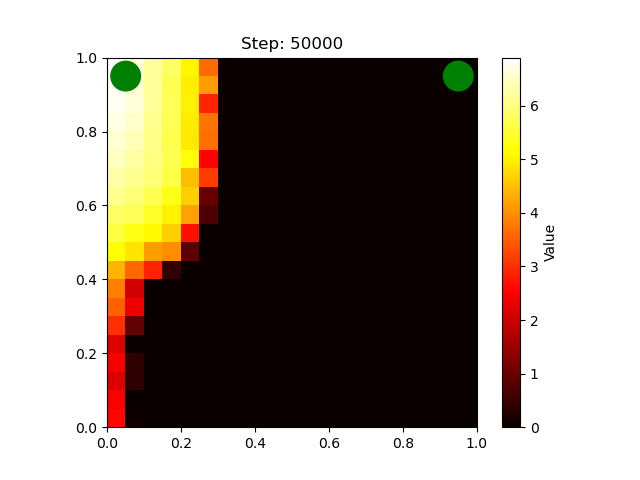
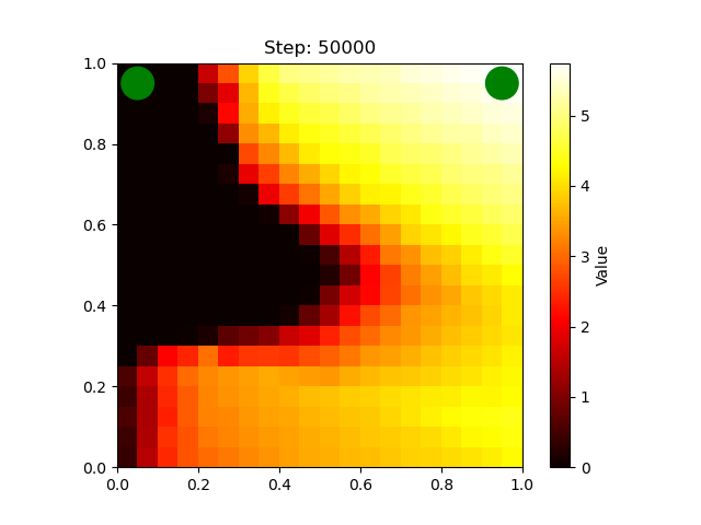
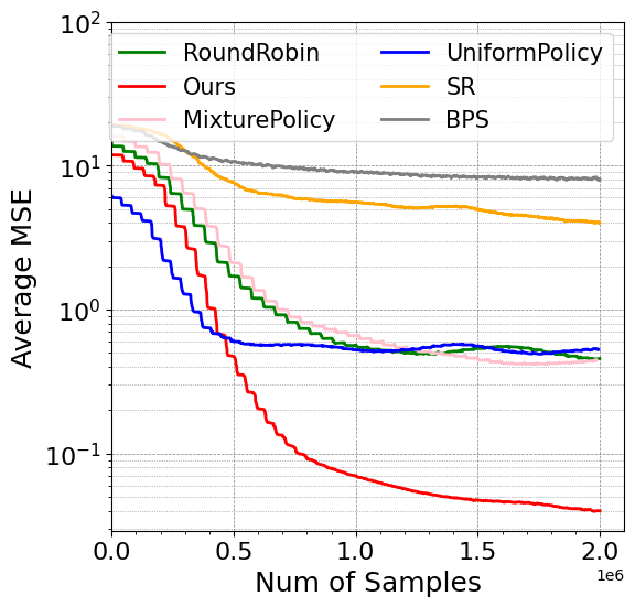
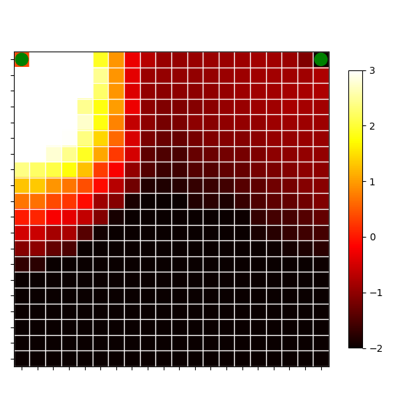
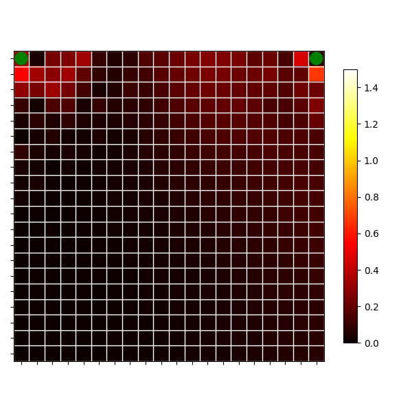
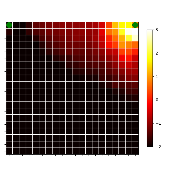
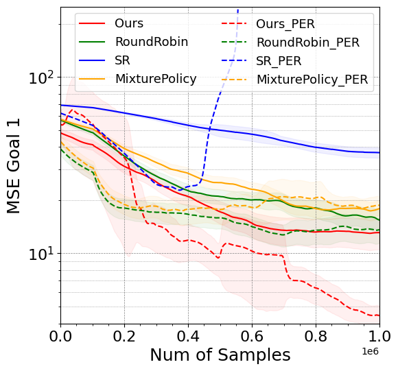
Next, in (Setting 2), we evaluate two GVFs, each with a different target policy-cumulant pairs. For GVF1, the cumulant is assigned to the top-left corner with zero elsewhere, while GVF2 receives at the top-right corner only. Figure 2 presents the comparison of MSEs for different algorithms; GVFExplorer produces better value estimates compared to the baselines. We also qualitatively analyse the results, by comparing baseline RoundRobin and GVFExplorer. In Figure 2(b,e) the plots depict the averaged absolute difference between true and estimated GVF values across states, . GVFExplorer leads to smaller errors (duller colors), especially around the high variance goal regions. In Figure 2(c,f) we show GVFExplorer’s estimated variance for GVF1 and GVF2, demonstrating high variance regions. This plot highlights the need for strategic non-uniform sampling, by focusing on high variance regions to minimize environmental interactions. These variance plots show log-scale empirical values; most areas appear black, due to their relatively small magnitude compared to high variance regions.


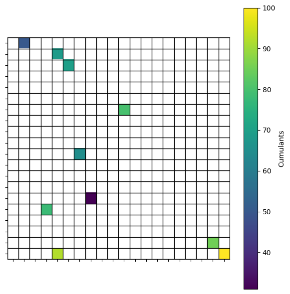
In the Setting 3, we evaluate our method’s ability to handle a large number of GVFs. We examine four target policies (), each aligned with a cardinal direction, and ten cumulants (), aiming to predict GVF combinations (). Each GVF is associated with a state space region (“goal”), uniformly sampled and assigned cumulant value ranging from to . The agent receives a zero cumulant signal on non-goal states. In Figure 3, we present a comparison of the average MSE across the various GVFs, illustrating the scalability of the proposed algorithm when increasing the number of GVFs. Notably, baseline SR shows limited scalability, because the varying cumulant scales affect the intrinsic behavior rewards (summation of SR weight change and reward weights). We omit BPS from this analysis due to its suboptimal performance in earlier experiments.
8.2 Continuous State Environment with Non-Linear Function Approximation
We use a Continuous GridWorld environment that extends the tabular experiments to a continuous state space (McLeod et al., 2021), and maintain four discrete cardinal actions. This environment is purposefully selected for its suitability in demonstrating meaningful and distinct GVF goals, offering a clearer qualitative analysis compared to more complex environments. We examine Setting 4 and consider two GVFs. The first GVF has a cumulant at the top-left corner and the second GVF has at the top-right corner , with zero cumulant assigned everywhere else. We used a constant discount . We used an Experience Replay Buffer with capacity and batch size for all the experiments. Further specifics on the computation of the true value functions using Monte Carlo and details on network architectures are provided in Section B.2.
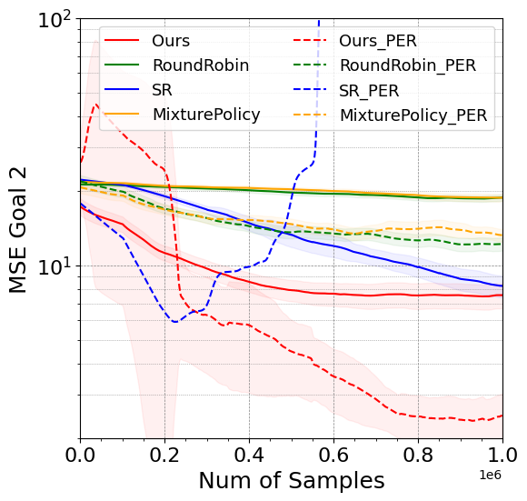
Prioritized Experience Replay (PER).
In our study, we also integrated Prioritized Experience Replay (PER) (Schaul et al., 2015) to evaluate the effectiveness of our algorithm. Unlike the standard Experience Replay Buffer which uniformly samples experiences, PER usually assigns priorities to samples based on the magnitude of the TD error in the Q-network. PER influences the weighting of samples during gradient updates without modifying the data collection process. In contrast, GVFExplorer adjusts the sampling strategy based on the total variance, defined as the expected cumulative discounted squared TD errors over time (refer Equation 6). GVFExplorer proactively uses future errors to adapt the sampling strategy. Whereas, PER focuses on one-step errors and only alters gradient updates without affecting the sampling strategy. Our method differs from PER in its independence from the replay buffer size ( or example, online learning in tabular experiments), offering flexibility with limited memory, while PER is known for diminishing performance with smaller buffer sizes.
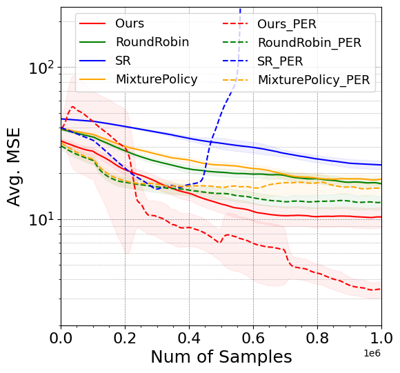
However, with further analysis, we found that PER is compatible with GVFExplorer, and in fact enhances its effectiveness. We use the absolute sum of TD errors across multiple GVF functions as a priority metric for PER in all the baselines, including GVFExplorer. We also conducted experimental trials using TD error of variance function to set the priority in GVFExplorer, but the results are not as good as the one obtained with priority on function’s TD error. In Figure 4, we present the MSE for both standard experience replay (solid lines) and PER (dotted lines) for all the algorithms. Interestingly PER reduces the MSE for most of the methods, but its integration with GVFExplorer offers a notable improvement. For the SR baseline, where the TD error in SR predictions is used as priority due to lack of a separate Q-network, we noted a substantial performance degradation. This suggests that the non-stationarity in the SRs’ TD errors under a dynamic behavior policy might lead PER to prioritize states that became less relevant under the current policy. The original SR work by McLeod et al. (2021) does not use PER in the experiments.
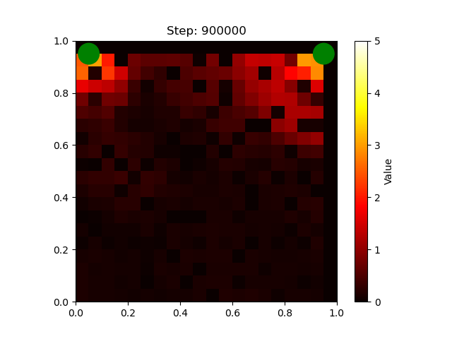
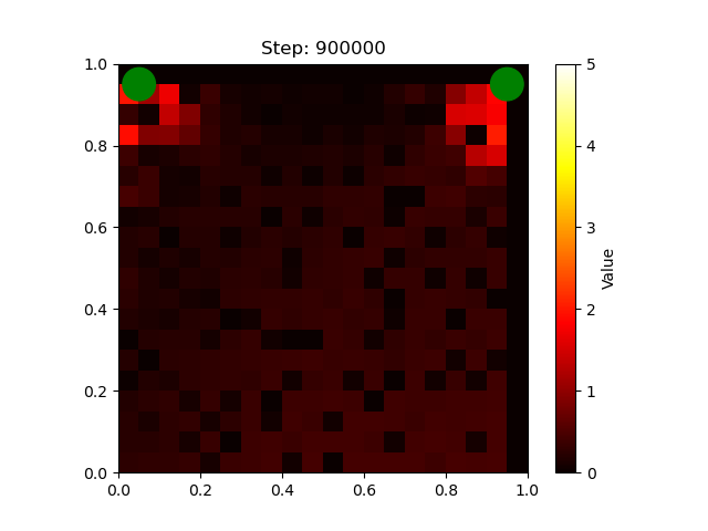
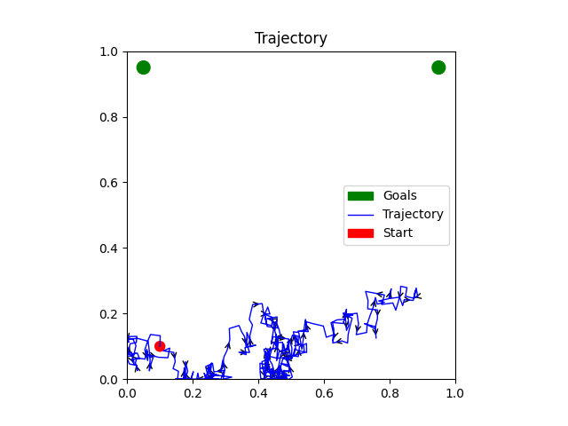
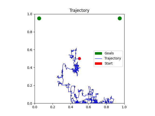
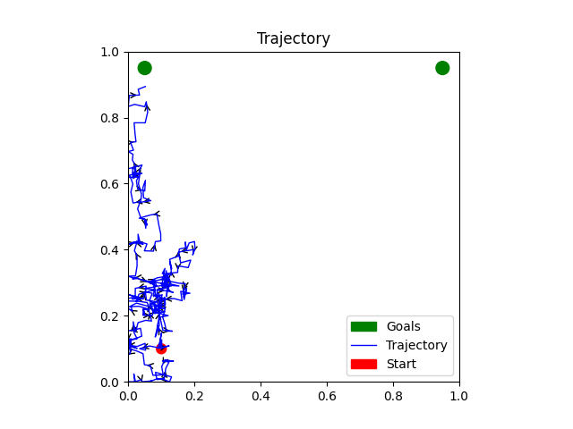
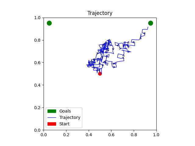
In Figure 5, we compare the absolute value errors for the baseline RoundRobin and GVFExplorer by discretizing the state space. Due to the objective of minimizing total MSE, we see smaller error magnitudes near the goals in GVFExplorer, indicating a focus on high-variance areas. Further insights into the variance estimation by GVFExplorer is shown in Section B.2. In Figure 6, GVFExplorer algorithm initially exhibits goal-directed behavior due to higher variability, resulting into faster cumulant propagation along other states. As the variance near the goals diminishes, the agent shifts its focus to other regions in descending order of variance, presenting a strategic data sampling approach. Finally, Table 1 summarizes the results highlighting the performance of various algorithms at steps.


| Avg MSE steps | SR | MixturePolicy | RoundRobin | GVFExplorer (Ours) | % Improvement of GVFExplorer (against best baseline) |
| Standard Replay Buffer | 21.7 | 18.25 | 16.78 | 5.19 | 69% |
| Prioritized Exp. Replay | 112 | 14.7 | 11.62 | 3.87 | 66% |
9 Discussion
In this work, we addressed the problem of parallel evaluations of multiple GVFs, each conditioned on a given target policy and cumulant. We developed a method to adaptively learn a behavior policy that uses a single experience stream to estimate all GVF values in parallel. The behavior policy selects actions in proportion to the total variance of the return across the multiple GVFs. This guides the policy to explore less known areas, thereby accelerating information flow and minimizing environmental interactions. We theoretically proved that each behavior policy update step reduces the total prediction error. Our empirical analysis showed the scalability of GVFExplorer for a large number of GVFs in a tabular setting and its ability to adapt to non-linear function approximation.
Limitations and Future Work.
One notable drawback of GVFExplorer is the increased time complexity, due to simultaneously learning two networks - one for value and the other for variance estimation. Additionally, GVFExplorer has not been evaluated in environments with significant range variations in cumulant functions. Disparities in cumulant ranges could lead to very different variances and potentially result in oversampling areas with higher cumulant values. Some calibration across cumulants may be necessary in such cases.
In this work we focused on minimizing the total MSE, but other loss functions, such as weighted MSE could also be considered. However, weighted MSE requires a priori knowledge about the weighting of errors in different GVFs, which is not readily available. A potential future direction could be to use variance scales to automatically adjust these weights, in order to provide uniform MSE reduction across all GVFs. Looking ahead, we are interested in testing our approach with multi-dimensional cumulants and general state-dependent discount factors, as well as, extending the applicability of GVFExplorer to control settings where the target policies are unknown.
References
- Bacon (2018) Pierre-Luc Bacon. Temporal Representation Learning. McGill University (Canada), 2018.
- Burda et al. (2018) Yuri Burda, Harrison Edwards, Amos Storkey, and Oleg Klimov. Exploration by random network distillation. arXiv preprint arXiv:1810.12894, 2018.
- Dayan (1993) Peter Dayan. Improving generalization for temporal difference learning: The successor representation. Neural computation, 5(4):613–624, 1993.
- Eysenbach et al. (2018) Benjamin Eysenbach, Abhishek Gupta, Julian Ibarz, and Sergey Levine. Diversity is all you need: Learning skills without a reward function. arXiv preprint arXiv:1802.06070, 2018.
- Frank et al. (2008) Jordan Frank, Shie Mannor, and Doina Precup. Reinforcement learning in the presence of rare events. In Proceedings of the 25th international conference on Machine learning, pp. 336–343, 2008.
- Guo et al. (2022) Zhaohan Guo, Shantanu Thakoor, Miruna Pîslar, Bernardo Avila Pires, Florent Altché, Corentin Tallec, Alaa Saade, Daniele Calandriello, Jean-Bastien Grill, Yunhao Tang, et al. Byol-explore: Exploration by bootstrapped prediction. Advances in neural information processing systems, 35:31855–31870, 2022.
- Hanna et al. (2017) Josiah P Hanna, Philip S Thomas, Peter Stone, and Scott Niekum. Data-efficient policy evaluation through behavior policy search. In International Conference on Machine Learning, pp. 1394–1403. PMLR, 2017.
- Hesterberg (1988) Timothy Classen Hesterberg. Advances in importance sampling. Stanford University, 1988.
- Jaderberg et al. (2016) Max Jaderberg, Volodymyr Mnih, Wojciech Marian Czarnecki, Tom Schaul, Joel Z Leibo, David Silver, and Koray Kavukcuoglu. Reinforcement learning with unsupervised auxiliary tasks. arXiv preprint arXiv:1611.05397, 2016.
- Jain et al. (2021) Arushi Jain, Gandharv Patil, Ayush Jain, Khimya Khetarpal, and Doina Precup. Variance penalized on-policy and off-policy actor-critic. In Proceedings of the AAAI Conference on Artificial Intelligence, volume 35, pp. 7899–7907, 2021.
- Kahn & Marshall (1953) Herman Kahn and Andy W Marshall. Methods of reducing sample size in monte carlo computations. Journal of the Operations Research Society of America, 1(5):263–278, 1953.
- Ladosz et al. (2022) Pawel Ladosz, Lilian Weng, Minwoo Kim, and Hyondong Oh. Exploration in deep reinforcement learning: A survey. Information Fusion, 85:1–22, 2022.
- Linke et al. (2020) Cam Linke, Nadia M Ady, Martha White, Thomas Degris, and Adam White. Adapting behavior via intrinsic reward: A survey and empirical study. Journal of artificial intelligence research, 69:1287–1332, 2020.
- Machado et al. (2017) Marlos C Machado, Clemens Rosenbaum, Xiaoxiao Guo, Miao Liu, Gerald Tesauro, and Murray Campbell. Eigenoption discovery through the deep successor representation. arXiv preprint arXiv:1710.11089, 2017.
- McLeod et al. (2021) Matthew McLeod, Chunlok Lo, Matthew Schlegel, Andrew Jacobsen, Raksha Kumaraswamy, Martha White, and Adam White. Continual auxiliary task learning. Advances in Neural Information Processing Systems, 34:12549–12562, 2021.
- Metelli et al. (2023) Alberto Maria Metelli, Samuele Meta, and Marcello Restelli. On the relation between policy improvement and off-policy minimum-variance policy evaluation. In Uncertainty in Artificial Intelligence, pp. 1423–1433. PMLR, 2023.
- Munos et al. (2016) Rémi Munos, Tom Stepleton, Anna Harutyunyan, and Marc Bellemare. Safe and efficient off-policy reinforcement learning. Advances in neural information processing systems, 29, 2016.
- Oudeyer et al. (2007) Pierre-Yves Oudeyer, Frdric Kaplan, and Verena V Hafner. Intrinsic motivation systems for autonomous mental development. IEEE transactions on evolutionary computation, 11(2):265–286, 2007.
- Owen (2013) Art B Owen. Monte carlo theory, methods and examples, 2013.
- Precup (2000) Doina Precup. Eligibility traces for off-policy policy evaluation. Computer Science Department Faculty Publication Series, pp. 80, 2000.
- Puterman (2014) Martin L Puterman. Markov decision processes: discrete stochastic dynamic programming. John Wiley & Sons, 2014.
- Rubinstein & Kroese (2016) Reuven Y Rubinstein and Dirk P Kroese. Simulation and the Monte Carlo method. John Wiley & Sons, 2016.
- Schaul et al. (2015) Tom Schaul, John Quan, Ioannis Antonoglou, and David Silver. Prioritized experience replay. arXiv preprint arXiv:1511.05952, 2015.
- Schlegel et al. (2021) Matthew Schlegel, Andrew Jacobsen, Zaheer Abbas, Andrew Patterson, Adam White, and Martha White. General value function networks. Journal of Artificial Intelligence Research, 70:497–543, 2021.
- Schmidhuber (2010) Jürgen Schmidhuber. Formal theory of creativity, fun, and intrinsic motivation (1990–2010). IEEE transactions on autonomous mental development, 2(3):230–247, 2010.
- Schulman et al. (2015) John Schulman, Sergey Levine, Pieter Abbeel, Michael Jordan, and Philipp Moritz. Trust region policy optimization. In International conference on machine learning, pp. 1889–1897. PMLR, 2015.
- Sherstan (2020) Craig Sherstan. Representation and general value functions. 2020.
- Sutton & Barto (2018) Richard S Sutton and Andrew G Barto. Reinforcement learning: An introduction. MIT press, 2018.
- Sutton et al. (2011) Richard S Sutton, Joseph Modayil, Michael Delp, Thomas Degris, Patrick M Pilarski, Adam White, and Doina Precup. Horde: A scalable real-time architecture for learning knowledge from unsupervised sensorimotor interaction. In The 10th International Conference on Autonomous Agents and Multiagent Systems-Volume 2, pp. 761–768, 2011.
- Watkins (2004) David S Watkins. Fundamentals of matrix computations. John Wiley & Sons, 2004.
- White et al. (2015) Adam White et al. Developing a predictive approach to knowledge. 2015.
- Williams (1992) Ronald J Williams. Simple statistical gradient-following algorithms for connectionist reinforcement learning. Machine learning, 8:229–256, 1992.
- Xu et al. (2022) Tengyu Xu, Zhuoran Yang, Zhaoran Wang, and Yingbin Liang. A unifying framework of off-policy general value function evaluation. Advances in Neural Information Processing Systems, 35:13570–13583, 2022.
Appendix A Proofs
See 5.1
Proof.
We formulate Equation 3 as a Lagrangian equation below to solve for the optimal behavior policy .
| (8) |
Here, and denotes the Lagrangian multipliers. The following KKT conditions satisfy:
-
1.
-
2.
-
3.
-
4.
-
5.
Gradient of .
The gradient of w.r.t. ,
Solving I part.
We will compute the gradient of in Equation 5 w.r.t to given . Here, is IS weight. We expand relation with to derive the gradient,
The final term is difficult to estimate in the off-policy setting. Hence, we are omitting (IV part) from the above gradient, which is similar to Jain et al. (2021), where the gradient of was omitted.
Solving for the Lagrangian Equation 8 further by substituting the (I part), and taking derivation of II & III part and using the (1) KKT condition.
| (9) |
From (2)KKT condition, we know that either or . Following the arguments of IS, support for can only be when the support for target policy . Solving for the case when support for target policy in non-zero, then let . We can simplify the gradient of Lagrangian in Equation 9,
| (10) | ||||
We know that the numerator is always positive (variance is positive), therefore . Let . From condition (5), we know that . Using Equation 10 and summing over all the actions we get,
Therefore, the update for optimal behavior policy becomes,
As the optimal policy appear on both the sides, this can be interpreted as an iterative update, where denotes the iterate number.
∎
See 5.2
Proof.
Theorem 5.1 suggests, for any given behavior policy, the next successive approximation minimizes the objective function Equation 3, i.e.,
| (11) | ||||
We will omit writing and assume that . Further, we will use the notation for ease of writing. From Equation 11, we can establish the relation,
| (12) |
Now, we will use Equation 12 relation to further simplify the equation and establish that variance decreases with every update step . We will use the notation to denote the products.
| (13) | ||||
∎
Definition A.1.
(Spectral Radius) The spectral radius of a matrix is denoted by , where denotes the eigenvalue of .
Lemma A.2.
The spectral radius of a matrix follows the relation, , where, is the infinity norm over a matrix.
Proof.
Following the derivation from Bacon (2018) Ph.D. thesis and work of Watkins (2004), we use the eigenvalue of a matrix to show that . We can write , when is the eigenvalue of . For any sub-multiplicative matrix norm, . Using this property,
The above is true for any eigenvalue of . So this must also be true for the maximum eigenvalue of . Therefore, we can express,
∎
Lemma A.3.
When the spectral radius of , then exits and is equal to,
Proof.
The proof for the Lemma is presented in Puterman (2014)[Proposition A.3]. ∎
See 6.1
Proof.
Following Lemma A.3, the inverse exists if spectral radius . Further, from Lemma A.2, we know that for any given matrix , spectral radius satisfies, . Hence, using the above two lemmas, we can express,
Further, if spectral radius satisfies the below condition, then the inverse exists,
We expand the middle infinity norm term and get
We can further express the above condition as ∎
Appendix B Experiments
We consider the two target policies with four cardinal directions left (L), right (R), up (U) and down (D) for the tabular and non-linear function approximation environments. These policies are specified as follows for every state :
| (14) |
B.1 Tabular Environment
We consider a tabular grid environment with stochastic dynamics. We use the target policies in Section B.1 for the different experimental settings. The Table 2 summarizes the averaged MSE with the same samples for different experimental settings.
| Avg MSE steps | BPS | SR | UniformPol | RoundRobin | MixPol | GVFExplorer (Ours) | % Improvement of Ours (against best baseline) |
| Distinct policies same cumulant | 26.13 | 2.76 | 1.22 | 1.15 | 1.15 | 0.24 | 79% |
| Distinct policies distinct cumulants | 8.2 | 4.1 | 0.54 | 0.47 | 0.44 | 0.04 | 91% |
| Large num of GVFs | - | 53.3 | 2.66 | 2.35 | 2.64 | 1.66 | 29% |
Hyperparameter Tuning:
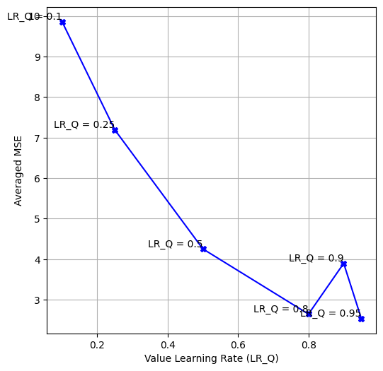
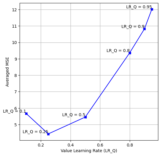
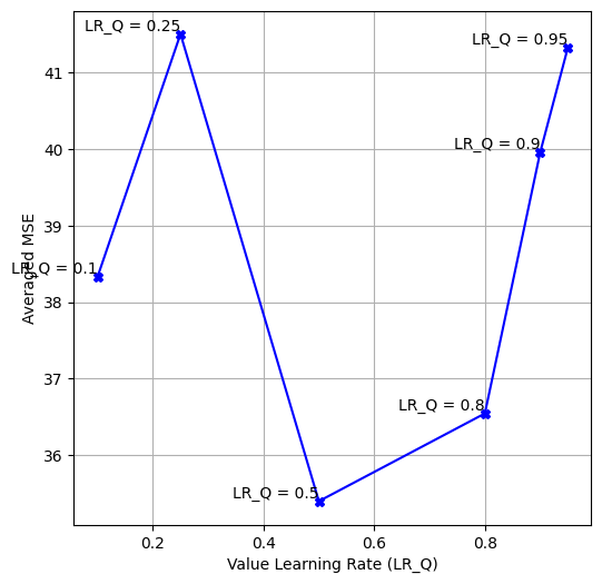
In our experiments, we use linearly decaying learning rates that starts with initial value of and gradually decreased to an optimized minimum value within steps of environmental interactions. We used different learning rates for value and variance function in GVFExplorer. The minimum learning rate parameter was swept within for both value and variance function. The optimal minimum learning rate was determined based on the one achieving the lowest average Mean Squared Error (MSE) after sample interactions. This hyperparameter tuning approach was consistently applied for all algorithms including baselines. Figure 7 shows the sensitivity analysis of varying learning rates for value functions (all baselines) and variance functions (our method) with the averaged MSE performance in experiment Setting 1 with distinct target policies and same cumulant. The learning rate resulting in the lowest MSE was selected as optimal. In Table 3, we show the optimal hyperparameters for the four experimental settings discussed in the paper earlier (refer Experimental Settings in Section 8).
Baselines.
(1) RoundRobin: We used a round robin strategy to sample data from all given target policies episodically. We used Expected Sarsa to estimate all GVF value functions in parallel when a transition is given as ,
(2) MixturePolicy, UniformPolicy are also evaluated using Expected Sarsa. (3)SR: (McLeod et al., 2021) Used a summation of weight change in SR and reward weights to get the intrinsic reward for behavior policy. Further Expected Sarsa is used over this intrinsic reward to learn the Q value function for behavior policy. Following the original work of McLeod et al. (2021), we use greedy policy over this behavior’s function to update the behavior policy. We use same learning rates for SR, reward weights and behavior policy Q function learning. (4)BPS: (Hanna et al., 2017) Use a Reinforce style estimator to learn , as mentioned in the original paper. Since, the original work is only about single policy evaluation, we extended for multiple GVFs by updating behavior policy as summation over . The behavior policy weight is updated as:

Experiment with Semi-greedy in 20x20 Grid :
In Setting 2, we evaluated semi-greedy target policies with distinct cumulants, and within a 20x20 grid. The target policies are designed with a bias towards top-left and top-right goals respectively,
| (15) | ||||
We keep the same cumulants as in previous experiments, on top-left corner and on top-right corner only, with cumulant everywhere else. In Figure 8, we compare the average MSE performance, where GVFExplorer exhibits comparable MSE to RoundRobin baseline but requires more samples to converge. This outcome can be attributed to the near-greedy nature of the target policies, which inherently guides RoundRobin along goal directed trajectories, enabling it to achieve nearly accurate predictions with fewer samples. The optimal hyperparameters for RoundRobin, UniformPolicy and MixturePolicy is . We used for ours GVFExplorer. Another baseline SR has and BPS as as optimal hyperparameters.
Experiment with high number of GVF predictions, Setting 3:
In this setting, we considered target policies in the four cardinal directions, namely:
We considered different cumulants, each with a single goal of constant reward at states uniformly choose from . The cumulant value is uniformly choosen between and is depicted in Figure 9. In total, the task is to predict GVF values. The experimental results are described in the main paper.
| Exp. Settings | Setting 1 | Setting 2 | Setting 3 | Setting 4 | ||||||||
| GVFExplorer (Ours) |
|
|
|
|
||||||||
| RoundRobin | 0.95 | 0.8 | 0.8 | |||||||||
| MixturePolicy | 0.95 | 0.8 | 0.8 | |||||||||
| UniformPolicy | 0.95 | 0.8 | 0.8 | - | ||||||||
| SR | 0.25 | 0.5 | 0.25 | |||||||||
| BPS | 0.5 | 0.8 | - | - |
B.2 Continuous State Environment with Non-linear Function Approximation
Continuous Environment.
We consider a Continuous GridWorld, similar to the tabular environment above, but with continuous state space (McLeod et al., 2021). It is a square-shaped environment with dimension and has four discrete actions similar as before. We consider two GVFs, similar to tabular Setting 2, where first GVF has cumulant at the left-top corner and second one has cumulant in top-right corner . The target policies are similar to one used in tabular environment before. Agent receives zero cumulant signal everywhere else. The agent moves with unit in the selected direction with an additional uniform noise . The agent can start randomly from anywhere, except it can not be within diameter of the goal state. The episode ends either when total steps are taken or agent reaches within diameter of the goal. In Figure 10 we show the estimated variance from each GVF separately, motivating the need to have a sampling strategy which prioritize high variance areas for reduced data interactions.
Computation of the true GVF values in continuous environment.
We compute the true GVF values in a continuous environment by using a Monte Carlo (MC) method. To manage the continuous states, we discretize the state space into a grid and select a continuous initial state from each such grid cell. We then calculate the average discounted return over trajectories that follow policy with cumulant . Finally, we assess the mean squared error (MSE) between the estimated and true GVF values using these same discretized states (), expressed as for all the algorithms.
Network Architecture.
We use distinct deep networks for learning value and variance . Both networks are similar. It has a shared feature extractor for input states and individual output heads for each GVF, yielding a multidimensional outputs for both value and variance. Additionally, variance network incorporates a softplus layer prior to each head’s output, guaranteeing a positive numerical values.