1]\orgdivDepartment Mathematics, \orgnameFriedrich-Alexander Universität Erlangen-Nürnberg (FAU), \orgaddress\streetCauerstr. 11, \cityErlangen, \postcode91058, \countryGermany
2]\orgdivCompetence Center for Scientific Computing (FAU CSC), \orgnameFriedrich-Alexander Universität Erlangen-Nürnberg (FAU), \orgaddress\streetMartensstr. 5a, \cityErlangen, \postcode91058, \countryGermany
3]\orgdivChair of Applied Mathematics, Continuous Optimization, Department Mathematics, \orgnameFriedrich-Alexander Universität Erlangen-Nürnberg (FAU), \orgaddress\streetCauerstrasse 11, \cityErlangen, \postcode91058, \countryGermany
4]\orgdivSchool of Applied Mathematics (FGV-EMAp), \orgnameFundação Getúlio Vargas, \orgaddress\streetPraia de Botafogo 190, \cityRio de Janeiro, \postcode22250-900, \countryBrazil
5]\orgdivInstituto de Matemática, \orgnameUniversidade Federal do Rio de Janeiro (UFRJ), \orgaddress\street Av. Athos da Silveira Ramos 149, \cityRio de Janeiro, \postcodeC.P. 68530, 21941-909, \countryBrazil
The obstacle problem for linear scalar conservation laws with constant velocity
Abstract
In this contribution, we present a novel approach for solving the obstacle problem for (linear) conservation laws. Usually, given a conservation law with an initial datum, the solution is uniquely determined. How to incorporate obstacles, i.e., inequality constraints on the solution so that the resulting solution is still “physically reasonable” and obeys the obstacle, is unclear. The proposed approach involves scaling down the velocity of the conservation law when the solution approaches the obstacle. We demonstrate that this leads to a reasonable solution and show that, when scaling down is performed in a discontinuous fashion, we still obtain a suitable velocity - and the solution satisfying a discontinuous conservation law. We illustrate the developed solution concept using numerical approximations.
keywords:
obstacle problem for conservation laws, obstacle problem, viscosity approximation, discontinuous conservation laws, solution constrained PDEpacs:
[MSC Classification]35L65,35L03,35L81,35N99
1 Introduction
1.1 The obstacle problem in the literature
Hyperbolic conservation laws involving constraints on the solution (usually called obstacles) arise naturally in many applications. For instance, in traffic modeling, it is natural to impose that vehicle density cannot exceed a certain threshold.
Bounds on the velocity can be envisioned, given by speed limits, or on the vehicular flux in a certain region [1, 2, 3, 4, 5, 6, 7, 8, 9, 10, 11]. Elsewhere, in multi-phase flows modeled by hyperbolic equations, constraints may appear in the solutions, leading to obstacles. For related problems involving hyperbolic settings, [12, 13, 14, 15, 16, 17, 18, 19] provide a few examples. In addition, pedestrian flows may involve congestion, so population density should be limited; see [20] for a recent survey.
More generally, in cases where the solution of a partial differential equation represents the density of a medium, e.g., a population, fluid, group of vehicles, or group of pedestrians, one may consider a variety of situations where a constraint on the density is imposed in a certain region of space or time. Therefore, since, in many cases, such dynamics are described by parabolic or hyperbolic evolution equations, a modeling mechanism capable of modifying an existing problem is useful to introduce density constraints in a meaningful way. This is especially interesting in cases where the solutions of the “free” problem (i.e., without constraint) typically violate the constraint; then, additional mechanisms that enforce the obstacle can be defined while remaining consistent with the underlying model.
The existing literature on obstacle problems is already substantial, especially concerning parabolic or elliptic problems. Since this is not the focus of our work, we cite only a few selected contributions, which are either foundational/surveys/monographs [21, 22, 23, 24, 25, 26, 27] or publications involving interesting applications [28, 29, 30]. Most approaches, especially in the parabolic setting, state the obstacle problem in a variational setting, where connecting the mathematical tools used to proper physical interpretations is not easy. Namely, a typical method to obtain a solution to an obstacle problem is by penalization. For instance, when a function that must remain below some obstacle is sought, the evolution equation is supplemented by some source terms acting to decrease on the set where in the setting of some approximation scheme. In general, though, such terms may have no ready interpretation in the model setting and often represent mathematical artifacts reminiscent of more abstract problems intended to find appropriate projections on convex sets [25, 21].
For hyperbolic conservation laws, in particular, the penalization approach has been applied by a few authors, e.g., [12, 17, 31]. One drawback is that a penalization term is, in general, not consistent with the conservation (or evolution) of the total mass. However, a constraint on a point-wise density should not necessarily affect the evolution of the total mass. In view of this, in the setting of an obstacle problem for a conservation law preserving mass, authors in [31] introduced a Lagrange multiplier (effectively a source term) designed to counterbalance the effect of the penalization on the total mass. However, the resulting formulation relies on mass creation and destruction to enforce the obstacle constraint while preserving the total mass. Here, we propose a different approach, which we argue is more natural.
Indeed, when trying to enforce an obstacle-like condition, density variations should originate from rearrangement of individuals rather than the destruction/creation of mass, especially in the case of traffic or pedestrian models. Thus, we expect that changes in the local velocity of the vehicles or individuals can be enough to adjust the density to satisfy the constraint. For a comparison of the two approaches, see Fig. 1.
With these remarks in mind, we propose a new formulation for the obstacle problem for a one-dimensional hyperbolic conservation law. In this work, we consider the case of a linear flux only. As shown below, the linear case allows for a cleaner exposition, focusing on the main innovations of our approach.
1.2 Problem statement and outline
The obstacle problems for linear conservation laws with constant coefficients reads
for an obstacle . As evident, the proposed system is over-determined in the sense that the Cauchy problem admits a unique solution without the obstacle. As a result, how to incorporate the obstacle into the solution is not straightforward when the following holds:
-
•
mass is conserved even when hitting the obstacle;
-
•
the solution still satisfies a semi-group property in time;
-
•
the solution behaves physically reasonably in the sense that mass is not instantaneously transported across space.
Having this in mind, one may need to adjust the velocity of the conservation law accordingly. Following this approach, we want the velocity of the conservation law to decrease when the solution approaches the obstacle. Thus, for a smoothed version of the Heaviside function , we consider the following nonlinear conservation law:
| (1) |
Here, the velocity becomes small when approaches , and whenever is not close to the obstacle, the dynamics evolve with the constant speed of (almost) as expected for the conservation law without the obstacle. However, the smoothness of remains problematic, as we indeed want the dynamics to hit the obstacle and only slow down when hitting it. Thus, the singular limit of the solution and the velocity is of interest as well as what values attains at this limit point, resulting in a discontinuous (in the solution) conservation law (compare, in particular, Rem. 5),
| (2) |
where denotes the Heaviside function. All the raised points are addressed in this manuscript, starting in Sec. 2 with the assumptions on the conservation law, the obstacle, and more (see Asm. 2). Additionally, as we deal with the viscous approximation of Eq. 1, we look into its well-posedness, i.e., existence and uniqueness of solutions.
In Sec. 3, we then show that the solutions to the viscosity approximation and Eq. 1 satisfy the obstacle constraint strictly as long as the initial datum is “compatible” and the density remains non-negative in the viscosity limit (for non-negative initial datum), uniformly in .
As we are interested in the mentioned convergence for , crefsec:Lipschitz presents one-sided Lipschitz (OSL) bounds for the solution and the velocity, uniformly in , from which we can conclude certain compactness properties of the solution and the velocity, culminating in the convergence result in Thm. 13. In addition, we show that even in the limit , the tuple satisfies a (discontinuous) conservation law, which is indeed of the form stated in Eq. 2.
Sec. 5 then characterizes the limit solution and velocity in specific, more restrictive setups, illustrating the reasonableness of the approach and providing insights into the limiting velocity. Surprisingly, the velocity does not become zero when the density approaches the obstacle. This phenomenon may seem counter-intuitive at first glance, but assuming that the velocity is zero, no mass is transported when the obstacle is active, i.e., a “full blocking” results once the obstacle is active. We also showcase how a backward shock front originating from the point of contact of the obstacle and the solution propagate.
Next, Sec. 6 continues to motivate the chosen approach for the obstacle problem, this time via optimization. On a formal level, we want to maximize the velocity of the conservation law at each point in time so the obstacle is not violated when forward propagating in time. This leads to an optimization problem for all time . We again see how the velocity behaves if the solution touches the obstacle, coinciding with the result in Sec. 5.
In Sec. 7, we conclude the contribution with numerical approximations by means of a tailored Godunov scheme, demonstrating the reasonableness of the approach and showing the approximate solution for some specific cases for a better understanding and intuition.
2 Preliminaries
First, we define a sequence of functions that approximates the Heaviside function smoothly and later plays an important role in approximating a solution to the obstacle problem. These functions should have the following properties:
Assumption 1 (Approximation of Heaviside function).
To approximate the Heaviside function, we consider a sequence for all , . Here, fulfills the following:
-
•
;
-
•
;
-
•
, for all ;
-
•
for all , and and all ;
-
•
it holds that
and
-
•
for all .
From the first point, we see that pointwise. The last point is not explicitly referenced again in this work. However, the assumption is not very restrictive and is used in the proof of Thm. 4.
To demonstrate that the above requirements are reasonable, the following is a simple example of such function .
Example 1 (Example of approximation).
We set , for , where satisfies all the properties outlined in Asm. 1.
Now, as stated in the introduction, we want to investigate Eq. 1 and its limiting behavior for and with initial condition . To proceed, assumptions about the regularity of the data are necessary.
Assumption 2 (Regularity).
Here denotes the space of functions with bounded variation and will denote the total variation (semi-norm).
Existence and uniqueness to Eq. 1 for can be found in the standard literature. We present the notion of solution (i.e., weak entropy solution) and a precise statement about existence and uniqueness.
Definition 1 (Entropy solution).
Given the definition of an entropy solution, we can state the existence and uniqueness of Eq. 1 as follows:
Theorem 3 (Existence and uniqueness to Eq. 1).
Proof.
To obtain quantitative estimates with regard to the parameter, we approximate Eq. 1 with a viscosity to work with smooth solutions, as detailed in the following
Definition 2 (Viscosity approximation).
The viscosity approximation approach has been laid out by, e.g., Kružkov [32]. However, it is not canonical to have on the right-hand side of a viscosity approximation. In fact, this term ensures the obstacle condition even for the viscosity approximation.
In the following, we state properties of the viscosity approximation and start with the well-posedness of Eqs. 3 to 4. For existence, we resort to parabolic theory.
Theorem 4 (Existence for the viscous equation Eq. 3).
Proof.
To prove this statement, we follow the steps in [35, Chapter II, Section 2] while extending the arguments to a space-dependent flux (as is our case).
To apply the results in [35], we first extend to a function such that and for some and for all .
The result is , and after obtaining the maximum principle Lem. 7, which is proved for first the extension as well, we obtain the result for Eq. 3. This is because will then only be evaluated on .
∎
Thanks to classical embedding theorems, we also obtain the following
Remark 1 (Asymptotic behavior of ).
Now, by embedding theorems, we have a classical solution of the viscous approximation. Thus, we can obtain bounds in as well as :
Theorem 5 (Estimates for ).
For , the solution to Eq. 3 satisfies
- bound:
-
- Spatial -bound:
-
For all , the following holds:
- -bound in time:
-
There exists such that for all ,
for all , where .
Even more, for monotonically decreasing , we even obtain uniform bounds in :
Remark 2 (Uniform bounds for monotone obstacles).
Let be decreasing and be the solution as in Eq. 3. Then, in and the following holds uniformly:
The case of increasing obstacles is trivial as the obstacle never becomes active.
Now, we have collected the necessary tools to prove that is indeed an entropy solution to Eq. 1:
Theorem 6 ( converges toward the entropy solution for ).
Proof.
The convergence of for on subsequences follows from Thm. 5 and the Riesz–Kolmogorov-type Theorem for Bochner spaces [37, Theorem 3]. Showing that is an entropy solution and by the uniqueness of entropy solution in Thm. 3, we indeed obtain convergence on all subsequences. This a standard argument that can be found in [32, p.236]. For this, must be bounded uniformly in . This is proven in Sec. 3. ∎
3 Comparison principles
Thm. 3 shows that respects the obstacle. However, we can even prove that the obstacle is never hit. This prevents the “full blocking”, as mentioned in the introduction.
Lemma 7 (Maximum principle/Obstacle is respected).
Let be a solution to Eq. 3 for . Then,
| (5) |
Proof.
First, extend to as discussed in the proof of Thm. 4. Let be the solution to
| (6) | |||||
| (7) |
Not only will we obtain the maximum principle for , but the maximum principle also implies that solves Eqs. 3 and 4:
Fix . In the end, we want to use [38, Theorem 1]. Here, must be differentiable a.e. Fortunately, this is guaranteed by Lipschitz continuity of all involved functions. Moreover, has to exist, and has to hold, both of which can be seen by invoking Asm. 2 and Rem. 1.
In the spirit of [38, Theorem 1], set
for . Set for and choose any .
Then, as a first case, if , we have
| (8) |
In the second case, if , then, according to standard optimality conditions [39, Chapter 2], we obtain
| (9) |
Then, we can differentiate as follows:
| Using Eq. 9, | ||||
Now, , and exists for all because of Asm. 2 and Rem. 1. Similarly,
Altogether, [38, Theorem 1] is applicable, and combining both cases for a.e. and all yields
Now, consider the Cauchy problem for the corresponding differential equation (instead of the inequality)
on that uniquely defines on because is globally Lipschitz (see Asm. 1). Since and , for all because equilibria are not allowed to be crossed. We also note that does not depend on ! Then, the ODE comparison principle (see, e.g., [40, Lemma 1.2, p.24]) implies for ,
This yields the claim. ∎
So, in fact, the obstacle is not even hit at all for , which also implies that the mass is transported with a positive velocity.
The same argument also allows for the proof of a minimum principle:
Theorem 8 (Minimum principle).
Proof.
The proof is similar to the previous one that shows that the obstacle is respected. It is again based on [38, Theorem 1]. ∎
Of note, the solution can be negative for ; however, in the limit, it will satisfy the expected lower bound of .
This also allows us to state bounds for the entropy solution:
Remark 3 (Bounds on entropy solution).
Let . Because -convergence implies point-wise convergence a.e. of a subsequence, the entropy solution from Thm. 6 fulfills the bounds
This can be obtained by letting in Eq. 10 and Eq. 5 point-wise a.e.. Here, we note that an upper bound exists on such that and does not depend on , as stated in the proof of Lem. 7. This allows for the strict inequality to hold pointwise a.e.
4 OSL bounds for and uniformly in
As stated earlier, the condition gives uniform -bounds of in and . We now want to find OSL bounds that provide a more general compactness result in , . We need the following:
Lemma 9 (OSL bounds and compactness).
Let be open and be a sequence of functions such that
Then, for every compact , and there exist and a subsequence such that
Proof.
First, we prove that is finite and does not depend on for every compact . Let be compact, and a compact interval . Set and for any .
Consequently, , and per [41, Theorem 13.35], the classical compactness result for functions of bounded variation gives convergence to in along a subsequence. ∎
Note that the result from Lem. 9 also holds if instead of . To obtain this, replace with and use Lem. 9.
Unfortunately, linear conservation laws have no intrinsic “smoothing” because of the lack of Oleinik-type estimates. However, as we later want to pass to the limit nevertheless, we impose an OSL condition on the initial datum, which is preserved over time (the same cannot easily be obtained with a argument).
Assumption 10 (Initial datum revisited).
In the following, we derive OSL bounds for uniform in :
Theorem 11 (OSL condition for in space).
There exists with such that with , and it holds that
where the right-hand side term is bounded thanks to Asm. 10.
Consequently, with —see Asm. 2— with and ,
Here, is interpreted as the lower OSL bound of .
Proof.
As before, we apply [38, Theorem 1]. Let
and for all . Choose . We distinguish two cases:
The first case is . Here,
since Eq. 8 and as in Asm. 2.
The second case is . Once again, optimality conditions lead to
| (12) |
and we then obtain
| Plugging in the strong form Eq. 3, we have | ||||
| We write for the positive and negative parts, respectively, and incorporate : | ||||
| Per Asm. 2, holds for , and we estimate as follows | ||||
| According to Eq. 10, there exists s.t. for all . Because , holds, so we can continue the estimate as | ||||
Applying [38, Theorem 1] and combining both cases, we obtain, for a.e. ,
Then, fix any . Now, if , we have a desirable lower bound on .
However, if , then . So,
holds, which implies, after integration,
which is the claimed inequality. Here, we remind the reader that is assumed in Eq. 11. ∎
A similar result can be derived for the velocity .
Theorem 12.
(OSL condition for in space) Let , be a solution to Eq. 3. Then, for fixed , there exists with such that
for all , , where
| (13) | ||||
| (14) | ||||
| (15) | ||||
| (16) | ||||
| (17) | ||||
| (18) |
Proof.
As before, we want to invoke [38, Theorem 1]. Fix and . Since
for all , from and the boundedness of , we obtain
The same argument can be employed for derivatives thereof. Therefore, [38] is indeed applicable.
Now, choose , where
We distinguish two cases.
- Case 1:
- Case 2:
-
For the sake of clarity, we (have to) introduce the following abbreviations (for , multi-index ):
Note that needs to be sharply distinguished from ; see also Asm. 1. Moreover, the notation is a bit misleading, as it still depends on . For , however, we have uniform -bounds in , which further motivates omitting the index.
In the following, we sometimes write rather than, e.g., , i.e., without its argument. Remember that is defined so that ,
So, based on standard optimality conditions, the following must hold:
(19) Expanding the above expressions (in the abbreviated notation), we obtain
and setting yields
(20) We apply Eq. 19 to Eq. 20, use twice, , and expand to arrive at the estimate (21) Using Eq. 19 as well as the identities and , we obtain and eventually replacing with in most cases yields We factor out for several expressions. Additionally, for according to Thm. 11, we have independent of (see Eq. 25) such that for all . Therefore, we can estimate if is sufficiently small: (22) (23)
Therefore, combining both cases, we show that by using [38, Theorem 1], for a.e. ,
| (24) |
Again, two cases have to be distinguished. For this, fix such that is differentiable (this is possible a.e.).
-
•
Case 2.1: () In this case, a bound on can be obtained immediately without Eq. 24: Choose some such that . If we choose as in Thm. 11, then from Thm. 11,
(25) holds. Here, . Then, we can estimate the following:
where and that is decreasing. Since the infimum of is positive per Asm. 2, the last expression has a uniform bound in . Namely,
(26) where .
-
•
Case 2.2: : Here, we estimate Eqs. 22 and 23 (once again in the abbreviated notation) using and :
Recall and the estimates from the fifth point of Asm. 1 to control the quotients. We set , factor out and estimate the other terms roughly: We additionally require to get remove . Let be as in Eq. 17. If , a feasible bound is found. If , then one can compute . In particular, . So, we estimate for this case Thus, if a maximal interval exists such that with as in Eq. 17 and for all , then Eq. 24 becomes for a.e. , whence
If no such interval exists, then, by continuity, stays below the maximum and the bound computed in Eq. 26.
Finally, in all cases, we obtain that
with defined as in Eq. 18. It remains to prove that is bounded uniformly in , which is a consequence of
where , which completes the proof. ∎
The obtained results allow us to pass to the limit, i.e., :
Theorem 13 (Convergence of and ).
Proof.
This follows from Theorems 5, 6, 9 and 11. ∎
Remark 4 (Missing time compactness of to obtain strong convergence).
Note that thanks to Thm. 12, one obtains by Lem. 9 total variation estimates of in a space uniform in . However, we could not obtain the required (compare [37, Theorem 3]) time compactness for strong convergence in , but we are left with a weaker form of convergence: Either the weak-star convergence in Thm. 13 or, for every , there exists and a sequence with such that
Indeed, is OSL-bounded from above (see Thm. 12).
One may wonder what the velocity and solution satisfy in the limit. This is characterized in the following:
Lemma 14 (Dynamics of the solution and velocity in the limit ).
The sequence of Thm. 13 satisfies in the limit the following weak form of a conservation law for :
| (27) |
Proof.
This is a direct consequence of Thm. 13 together with the fact that the product of a strongly and a weakly-* convergent sequence converges weak-*. ∎
Remark 5 (Discontinuous conservation laws/relation to Lem. 14).
Looking back to the regularized obstacle problem in Eq. 1, this equation converges to a discontinuous (in the solution and spatial variable (!)) conservation law as the velocity converges to a discontinuous function, i.e.,
and thus, we obtain
| (28) |
where is a test function as in Lem. 14 and is the Heaviside function with a value at zero that is undetermined, i.e., can attain any value in . One may wonder whether applying results on the uniqueness of these discontinuous conservation laws is possible [42, 43, 44, 45, 46, 47]; however, the discontinuous conservation law considered here does not seem to fit into the required frameworks.
5 Characterization of the limit in specific cases
This section presents characterizations of the solutions approached in Thm. 13 under additional assumptions on its smoothness and more. They serve to build an intuition on what happens in this limit as well as how the dynamics behave at the obstacle.
Suppose we have a solution as in Eq. 27 that is piecewise smooth in the sense that it is smooth outside of a finite number of curves in , across which or has jump discontinuities. We take a representative that is also piecewise smooth, such that and have well-defined traces at every point of discontinuity and the coincidence set , is of the form
for two continuous piecewise smooth curves on with non-decreasing. Suppose there exists a well-defined first collision time. We can set it without loss of generality to be (this is a contradiction to Asm. 2 as we postulated ; however, thanks to the semi-group property of any conservation law, we can shift time accordingly).
Then, the following result relying on the Rankine–Hugoniot condition [48, 49] gives a characterization of the boundary curves of the coincidence region in terms of the traces of and from the outside of :
Theorem 15.
Assume that and adhere to Asm. 2, is strictly decreasing on some interval , and the limits for ,
exist for a.e. point along the curves . Suppose further that is uniformly bounded on the (open) set . Under the previous assumptions, we have the following:
-
1.
The velocity field as in Lem. 14 (and thus the speed of the characteristics) is given by
(29) -
2.
, holds, and
(30) -
3.
In intervals where is differentiable, either , or if is smooth at ,
(31) which, if has a jump discontinuity at , results in
(32)
In particular, has a discontinuity along . When , then is the speed of a backward congestion shock originated by the collision with the obstacle.
Proof.
Consider a sufficiently small open ball centered on a point where is smooth. Let and set with obvious notation (see Fig. 2).
Take a test function supported in . Since is a distributional solution of the conservation law in we have (here, for the sake of brevity, we omit the arguments of the functions)
| as , and we obtain | ||||
| (33) | ||||
Let us look at each of the two integrals in turn. First, note that in the coincidence set , the obstacle is a distributional solution of
| (34) |
Since does not depend on , we conclude that is the zero distribution on . Therefore, owing to distribution theory, the function is constant in for almost all . Thus, holds a.e. on for a.e. .
To identify , we recall that is OSL continuous from below in the spatial variable (see Thm. 12 and apply the limit) uniformly in . Let us see that, actually,
Let be this Lipschitz constant. Writing , observe that for a.e. for which are defined, and :
As , we obtain that the left-hand side converges to since (see the definition of ), whereas as . So, in total,
for all , whence for a.e. . Thus, plug into to obtain . This proves the representation Eq. 29.
Going back to Eq. 33, we deduce for the first integral, using the divergence theorem (let denote the surface measure),
For the second integral in Eq. 33, we find again with the divergence theorem and the fact that on , satisfy the transport equation,
Therefore, the following holds:
Since is arbitrary, we conclude that
| (35) |
for a.e. exploiting the given structure of and the fact that the center of is arbitrary.
Now, suppose that and is strictly smaller than . Then, from the strict monotonicity of and Eq. 35, we have , which is absurd. Therefore, , and Eq. 30 follows by rearranging.
Eqs. 32 and 31 remain to be proven. Suppose that has a jump discontinuity at . Then, by assumption, there exists the trace and, necessarily, . The proof of Eq. 32 is entirely analogous to the proof of Eq. 30, but instead of Eq. 35, we obtain
and thus, since .
Suppose now that is continuous at , has a trace from the right, , and . Then, , which implies that . Observe that necessarily, . The formal calculation to show Eq. 31 is as follows. Compute the derivative of along the curve to find . But, along , holds; therefore, using Eq. 34 for on ,
| (36) | ||||
giving Eq. 31. However, while is differentiable, is not differentiable at , and so, the calculation is not justified. To circumvent this problem, a more careful computation is needed, which we now provide.
Let and consider the quantity
On the one hand, we have
| (37) |
On the other hand, we find
| (38) |
The first term gives
as , from our smoothness assumptions on from outside of . Note that we can use the transport equation for since is outside the coincidence region . For the second term in Eq. 38, we find
Now, clearly the first term converges to when , while the second can be easily bounded by , which also vanishes in the limit .
Therefore, which together with Eq. 37 gives the rigorous analogue of Eq. 36. Thus, we find that
Finally, recalling that we obtain Eq. 31 by rearranging. This completes the proof.
∎
6 Motivation of velocity for by optimization
The result from Thm. 15 can also be formally motivated from an optimization perspective. We can, in fact, demonstrate that the velocity , found in the previous chapter, is maximal in an sense for each time.
To this end, let us first assume that the density moves with a space- and time-dependent velocity (the choice of this dependency becomes clear later) while obeying the scalar conservation law
| (39) |
The conservation laws’ characteristics emanating from , i.e., are given as a solution of the ODE (see, e.g., [50, Sec. 2]):
| (40) |
We assume that is OSL from below in the spatial variable and essentially bounded in . According to [50, 51], the solution to Eq. 39 satisfies
for all and . The previously mentioned solution formula makes the semi-group property (in time) of the dynamics visible.
We then define the -obstacle violation by introducing the function for all and choose a :
| (41) | ||||
| Performing a substitution according to Eq. 40, i.e., , we obtain | ||||
with . Thanks to the previously assumed regularity, we can compute the time-derivative and obtain the following by applying the chain rule for :
| and substituting according to Eq. 40, | ||||
| (42) | ||||
This yields, in particular (recalling again the properties of the characteristics in Eq. 40),
| (43) |
On an abstract level, we have the function measuring the violation of the obstacle. We also have (the initial datum respects the obstacle) that . If we can manage to show that
| (44) |
we know that the obstacle is never violated, i.e, .
Thus, assume there exists such that . Then, there exists measurable with Lebesgue-measure greater zero so that
Recalling Eq. 43, we have
and so, we obtain by postulating Eq. 44 in a weak sense that
If we keep in mind that we want the velocity at time to be maximal in some topology, we obtain the optimization problem (in )
| (45) | ||||||
| subject to | ||||||
where the inequality constraint is meant distributionally.
For sets that are irregular (e.g., Cantor sets), the authors are unccertain on how to characterize solutions to the Eq. 45, but if this could be established, it may even present a more direct way to “solve the obstacle problem.” However, assuming that the set is a union of disjoint intervals for an index set , we can solve on each on these intervals Eq. 45.
Theorem 16 (The solution to Eq. 45).
For , the optimality system in Eq. 45 with the additional assumption that, for an index set and a set of disjoint intervals ,
admits a unique solution
This characterizes the velocity at time so that one can see the solution to the obstacle as the solution of the conservation law
The choice of considering the solution on characteristics Eq. 41 is due to our requiring the expression to be time-sensitive concerning the obstacle violation and differentiable.
Remarkably, under the assumptions in Thm. 16, the characterization of the velocity coincides with the results in Sec. 5, namely, Eq. 29. This underlines the reasonability of the proposed approach, as in a regular enough setting, all presented approaches (regularization in in Sec. 4, characterization by Rankine–Hugoniot type approach in Sec. 5, and the optimization approach in this Sec. 6) coincide.
7 Visualization by means of a tailored Godunov scheme
In this section, we conduct numerical studies to “validate” the theoretical results about properties of the solution to Eq. 1, i.e.,
on with initial condition , . Here, if not stated otherwise, is as in Ex. 1, i.e., , and ,
| (46) | ||||
| for all and the corresponding initial data | ||||
| , | ||||
| (47) | ||||
for all . Of note, (due to nondifferentiability) and (due to lack of Lipschitz bounds) are not in accordance with Asm. 2.
To simulate Eq. 1, we employ a space-dependent Godunov method as laid out in [52, (34)] but use an adaptive step size such that a Courant-Friedrichs-Lévy-type condition (for non–space-dependent flux case, see [53, (13.11)]) holds in every time step.
For the spatial step size, we chose . The adapted temporal step size then leads to several million time steps in every instance.
7.1 Visualization of for different scenarios
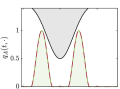
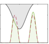
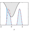
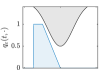
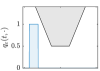
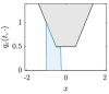
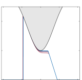
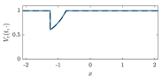
In Sec. 7.1, we let and observe the behavior of for different obstacles and initial data. Choosing as the obstacle and as the initial datum, we obtain the result in Fig. 3. Density accumulates “in front of” the obstacle, which can be interpreted as a “traffic jam”. Also, density uses almost all the possible space under . In Fig. 4, we offer some more perspectives that also indicate very clearly that the obstacle is obeyed.


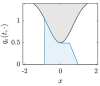


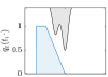
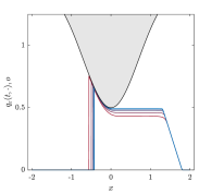
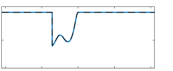
Choosing the data and , we obtain the results portrayed in Fig. 5.


In fact, the lack of regularity of this data does not prevent the solution from behaving in a physical/intuitive manner. However, at and , some minor diffusion effects can be observed in the sense that the solution seems to “fade out” to its right. This is a numerical problem and would be far greater if one employs a Lax–Friedrichs scheme [52, p.16] instead of a Godunov scheme.
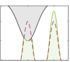
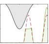
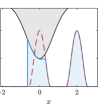
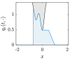
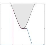
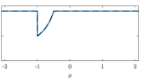
The obstacle in the case of and (see Fig. 6) is a little more delicate. Still, the solution behaves in the desired manner. Once the first stalactite of the obstacle is passed, the density between the two stalactites only starts to increase once the second one is hit. After some time, all the “room” is used by the solution.


7.2 as
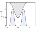
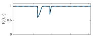
To observe the behavior of with becoming very small, we simulate Eq. 1 with initial datum and obstacle for several different , as shown in Fig. 7.
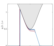
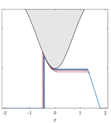
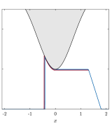
We see that for smaller , the solution moves closer to the obstacle. This becomes especially evident around the point . This behavior can be motivated by the fact that as on (recall Asm. 1). So, the smaller , the later slows down.
Thus, as suggested in Thm. 13 1), the convergence of as can be identified numerically.
Moreover, if we choose a different regularization of , namely, or (see Fig. 7), we see the same behavior. Note that the latter function (e.g., due to non-differentiability) does not meet the requirements in Asm. 1. In fact, the solutions for larger are closer to the solution for than in Fig. 7. This is due to the -regularization being more precise.
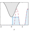
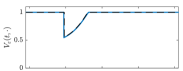
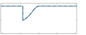
7.3 Visualization of
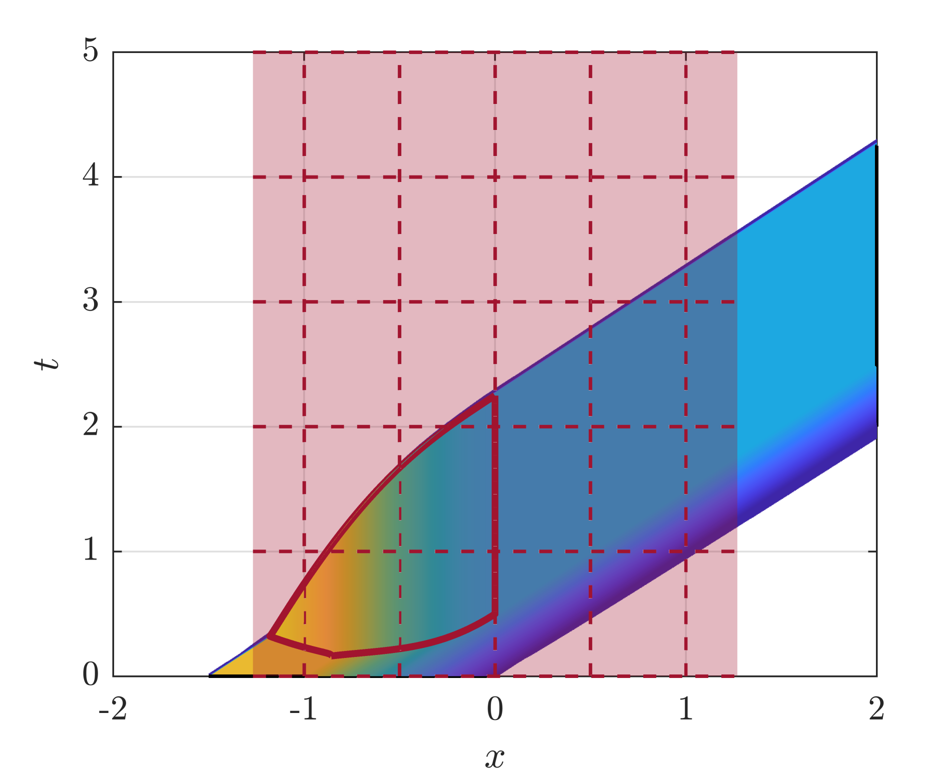
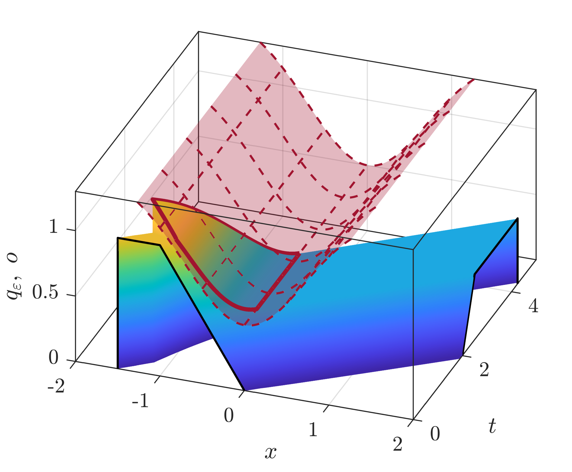
Motivated by Thm. 15, we hypothesize that if and there exists an interval such that on , holds for all , where . As we can not compute , we want to analyze for the small value of . In fact, at least numerically, our examples in Fig. 8 show the desired behavior.
8 Open problems—future research
The most important question not answered in this work is whether the solution to Eq. 28 is unique and if it is independent of the regularization .
Moreover, several generalizations are straightforward to some degree:
-
•
The same approach works if we do not assume a constant velocity if the obstacle is not present but rather a space- and time-dependent velocity satisfying required regularity for well-posedness.
- •
-
•
The same argument can be made for nonlocal conservation laws [50].
-
•
In the case of systems of conservation laws [54] and multi-d conservation laws, the presented approach may require some refinement. Particularly in the multi-d case, researchers may choose to steer toward the direction of the velocity field, which cannot be represented by a simple rescaling.
Data Availability
There is no associated data.
Acknowledgments
L. Pflug and J. Rodestock have been supported by the DFG – Project-ID 416229255 – SFB 1411.
References
- \bibcommenthead
- Berthelin et al. [2007] Berthelin, F., Degond, P., Delitala, M., Rascle, M.: A model for the formation and evolution of traffic jams. Archive for Rational Mechanics and Analysis 187(2), 185–220 (2007) https://doi.org/10.1007/s00205-007-0061-9
- Andreianov et al. [2016a] Andreianov, B., Donadello, C., Razafison, U., Rosini, M.D.: Qualitative behaviour and numerical approximation of solutions to conservation laws with non-local point constraints on the flux and modeling of crowd dynamics at the bottlenecks. ESAIM Math. Model. Numer. Anal. 50(5), 1269–1287 (2016) https://doi.org/10.1051/m2an/2015078
- Andreianov et al. [2016b] Andreianov, B., Donadello, C., Rosini, M.D.: A second-order model for vehicular traffics with local point constraints on the flow. Math. Models Methods Appl. Sci. 26(4), 751–802 (2016) https://doi.org/10.1142/S0218202516500172
- Chalons et al. [2013] Chalons, C., Goatin, P., Seguin, N.: General constrained conservation laws. Application to pedestrian flow modeling. Netw. Heterog. Media 8(2), 433–463 (2013) https://doi.org/10.3934/nhm.2013.8.433
- Berthelin [2002] Berthelin, F.: Existence and weak stability for a pressureless model with unilateral constraint. Math. Models Methods Appl. Sci. 12(2), 249–272 (2002) https://doi.org/10.1142/S0218202502001635
- De Nitti et al. [2024] De Nitti, N., Serre, D., Zuazua, E.: Pointwise constraints for scalar conservation laws with positive wave velocity. cvgmt preprint (2024). http://cvgmt.sns.it/paper/6472/
- Colombo and Goatin [2007] Colombo, R.M., Goatin, P.: A well posed conservation law with a variable unilateral constraint. J. Differential Equations 234(2), 654–675 (2007) https://doi.org/10.1016/j.jde.2006.10.014
- Dymski et al. [2018] Dymski, N.S., Goatin, P., Rosini, M.D.: Existence of solutions for a non-conservative constrained Aw-Rascle-Zhang model for vehicular traffic. J. Math. Anal. Appl. 467(1), 45–66 (2018) https://doi.org/10.1016/j.jmaa.2018.07.025
- Garavello and Goatin [2011] Garavello, M., Goatin, P.: The Aw-Rascle traffic model with locally constrained flow. J. Math. Anal. Appl. 378(2), 634–648 (2011) https://doi.org/10.1016/j.jmaa.2011.01.033
- Garavello and Villa [2017] Garavello, M., Villa, S.: The Cauchy problem for the Aw-Rascle-Zhang traffic model with locally constrained flow. J. Hyperbolic Differ. Equ. 14(3), 393–414 (2017) https://doi.org/10.1142/S0219891617500138
- Bayen et al. [2022] Bayen, A., Friedrich, J., Keimer, A., Pflug, L., Veeravalli, T.: Modeling multilane traffic with moving obstacles by nonlocal balance laws. SIAM Journal on Applied Dynamical Systems 21(2), 1495–1538 (2022) https://doi.org/10.1137/20m1366654
- Levi [2001] Levi, L.: Obstacle problems for scalar conservation laws. M2AN Math. Model. Numer. Anal. 35(3), 575–593 (2001) https://doi.org/%****␣main_42.bbl␣Line␣225␣****10.1051/m2an:2001127
- Rodrigues [2004] Rodrigues, J.F.: On hyperbolic variational inequalities of first order and some applications. Monatsh. Math. 142(1-2), 157–177 (2004) https://doi.org/10.1007/s00605-004-0238-3
- Rodrigues [2002] Rodrigues, J.F.: On the hyperbolic obstacle problem of first order. vol. 23, pp. 253–266 (2002). https://doi.org/10.1142/S0252959902000249 . Dedicated to the memory of Jacques-Louis Lions. https://doi.org/10.1142/S0252959902000249
- Goudon and Vasseur [2016] Goudon, T., Vasseur, A.: On a model for mixture flows: derivation, dissipation and stability properties. Arch. Ration. Mech. Anal. 220(1), 1–35 (2016) https://doi.org/10.1007/s00205-015-0925-3
- Saldanha da Gama et al. [2012] Gama, R.M., Pedrosa Filho, J.J., Martins-Costa, M.L.: Modeling the saturation process of flows through rigid porous media by the solution of a nonlinear hyperbolic system with one constrained unknown. ZAMM Z. Angew. Math. Mech. 92(11-12), 921–936 (2012) https://doi.org/10.1002/zamm.201100031
- Berthelin and Bouchut [2003] Berthelin, F., Bouchut, F.: Weak solutions for a hyperbolic system with unilateral constraint and mass loss. Ann. Inst. H. Poincaré C Anal. Non Linéaire 20(6), 975–997 (2003) https://doi.org/%****␣main_42.bbl␣Line␣300␣****10.1016/S0294-1449(03)00012-X
- Rossi et al. [2020] Rossi, E., Weißen, J., Goatin, P., Göttlich, S.: Well-posedness of a non-local model for material flow on conveyor belts. ESAIM: Mathematical Modelling and Numerical Analysis 54(2), 679–704 (2020) https://doi.org/10.1051/m2an/2019062
- Fernández-Real and Figalli [2020] Fernández-Real, X., Figalli, A.: On the obstacle problem for the 1d wave equation. Mathematics in Engineering 2(4), 584–597 (2020) https://doi.org/10.3934/mine.2020026
- Bellomo et al. [2022] Bellomo, N., Gibelli, L., Quaini, A., Reali, A.: Towards a mathematical theory of behavioral human crowds. Mathematical Models and Methods in Applied Sciences 32(02), 321–358 (2022)
- Lions and Stampacchia [1967] Lions, J.-L., Stampacchia, G.: Variational inequalities. Comm. Pure Appl. Math. 20, 493–519 (1967) https://doi.org/10.1002/cpa.3160200302
- Kinderlehrer and Stampacchia [1980] Kinderlehrer, D., Stampacchia, G.: An Introduction to Variational Inequalities and Their Applications. Pure and Applied Mathematics, vol. 88, p. 313. Academic Press, Inc. [Harcourt Brace Jovanovich, Publishers], New York-London (1980)
- Rodrigues [1987] Rodrigues, J.-F.: Obstacle Problems in Mathematical Physics. North-Holland Mathematics Studies, vol. 134, p. 352. North-Holland Publishing Co., Amsterdam (1987). Notas de Matemática, 114. [Mathematical Notes]
- Mignot and Puel [1976] Mignot, F., Puel, J.-P.: Inéquations variationnelles et quasivariationnelles hyperboliques du premier ordre. J. Math. Pures Appl. (9) 55(3), 353–378 (1976)
- Brézis [1972] Brézis, H.: Problèmes unilatéraux. J. Math. Pures Appl. (9) 51, 1–168 (1972)
- Rudd and Schmitt [2002] Rudd, M., Schmitt, K.: Variational inequalities of elliptic and parabolic type. Taiwanese J. Math. 6(3), 287–322 (2002) https://doi.org/10.11650/twjm/1500558298
- Korte et al. [2009] Korte, R., Kuusi, T., Siljander, J.: Obstacle problem for nonlinear parabolic equations. J. Differential Equations 246(9), 3668–3680 (2009) https://doi.org/10.1016/j.jde.2009.02.006
- Rodrigues and Santos [2012] Rodrigues, J.F., Santos, L.: Quasivariational solutions for first order quasilinear equations with gradient constraint. Arch. Ration. Mech. Anal. 205(2), 493–514 (2012) https://doi.org/10.1007/s00205-012-0511-x
- Chalub and Rodrigues [2006] Chalub, F.A.C.C., Rodrigues, J.F.: A class of kinetic models for chemotaxis with threshold to prevent overcrowding. Port. Math. (N.S.) 63(2), 227–250 (2006)
- Bögelein et al. [2011] Bögelein, V., Duzaar, F., Mingione, G.: Degenerate problems with irregular obstacles. J. Reine Angew. Math. 650, 107–160 (2011) https://doi.org/10.1515/CRELLE.2011.006
- Amorim et al. [2017] Amorim, P., Neves, W., Rodrigues, J.F.: The obstacle-mass constraint problem for hyperbolic conservation laws. Solvability. Ann. Inst. H. Poincaré C Anal. Non Linéaire 34(1), 221–248 (2017) https://doi.org/10.1016/j.anihpc.2015.11.003
- Kružkov [1970] Kružkov, S.N.: First order quasilinear equations in several independent variables. Mathematics of the USSR-Sbornik 10(2), 217 (1970) https://doi.org/10.1070/SM1970v010n02ABEH002156
- Alt [2016] Alt, H.W.: Linear Functional Analysis. Springer, London (2016). https://doi.org/10.1007/978-1-4471-7280-2 . http://dx.doi.org/10.1007/978-1-4471-7280-2
- Evans and Gariepy [2015] Evans, L.C., Gariepy, R.F.: Measure Theory and Fine Properties of Functions, Revised Edition. Chapman and Hall/CRC, Boca Raton (2015). https://doi.org/10.1201/b18333 . http://dx.doi.org/10.1201/b18333
- Godlewski and Raviart [1991] Godlewski, E., Raviart, P.A.: Hyperbolic Systems of Conservation Laws. Mathématiques & applications. Ellipses, Paris (1991). https://books.google.de/books?id=X3qyvAEACAAJ
- Brezis [2010] Brezis, H.: Functional Analysis, Sobolev Spaces and Partial Differential Equations. Springer, New York (2010). https://doi.org/10.1007/978-0-387-70914-7 . http://dx.doi.org/10.1007/978-0-387-70914-7
- Simon [1986] Simon, J.: Compact sets in the space . Annali di Matematica Pura ed Applicata 146, 65–96 (1986)
- Milgrom and Segal [2002] Milgrom, P., Segal, I.: Envelope theorems for arbitrary choice sets. Econometrica 70(2), 583–601 (2002) https://doi.org/%****␣main_42.bbl␣Line␣600␣****10.1111/1468-0262.00296
- Nocedal and Wright [2006] Nocedal, J., Wright, S.: Numerical Optimization. Springer, New York (2006). https://doi.org/10.1007/978-0-387-40065-5 . http://dx.doi.org/10.1007/978-0-387-40065-5
- Teschl [2012] Teschl, G.: Ordinary Differential Equations and Dynamical Systems. American Mathematical Society, Providence (2012). https://doi.org/10.1090/gsm/140 . http://dx.doi.org/10.1090/gsm/140
- Leoni [2009] Leoni, G.: A First Course in Sobolev Spaces. American Mathematical Society, Providence (2009). https://doi.org/10.1090/gsm/105 . http://dx.doi.org/10.1090/gsm/105
- BULÍČEK et al. [2011] BULÍČEK, M., GWIAZDA, P., MÁLEK, J., ŚWIERCZEWSKA-GWIAZDA, A.: On scalar hyperbolic conservation laws with a discontinuous flux. Mathematical Models and Methods in Applied Sciences 21(01), 89–113 (2011) https://doi.org/10.1142/s021820251100499x
- Bulíček et al. [2017] Bulíček, M., Gwiazda, P., Świerczewska-Gwiazda, A.: On unified theory for scalar conservation laws with fluxes and sources discontinuous with respect to the unknown. Journal of Differential Equations 262(1), 313–364 (2017) https://doi.org/10.1016/j.jde.2016.09.020
- Carrillo [2003] Carrillo, J.: Conservation laws with discontinuous flux functions and boundary condition. Journal of Evolution Equations 3(2), 283–301 (2003) https://doi.org/10.1007/s00028-003-0095-x
- Martin and Vovelle [2008] Martin, S., Vovelle, J.: Convergence of implicit finite volume methods for scalar conservation laws with discontinuous flux function. ESAIM: Mathematical Modelling and Numerical Analysis 42(5), 699–727 (2008) https://doi.org/10.1051/m2an:2008023
- Dias and Figueira [2005] Dias, J.-P., Figueira, M.: On the approximation of the solutions of the riemann problem for a discontinuous conservation law. Bulletin of the Brazilian Mathematical Society, New Series 36(1), 115–125 (2005) https://doi.org/10.1007/s00574-005-0031-5
- Dias and Figueira [2004] Dias, J.-P., Figueira, M.: On the riemann problem for some discontinuous systems of conservation laws describing phase transitions. Communications on Pure & Applied Analysis 3(1), 53–58 (2004) https://doi.org/10.3934/cpaa.2004.3.53
- Rankine [1870] Rankine, W.J.M.: Xv. on the thermodynamic theory of waves of finite longitudinal disturbance. Philosophical Transactions of the Royal Society of London 160, 277–288 (1870) https://doi.org/10.1098/rstl.1870.0015
- Hugoniot [1887] Hugoniot, H.: Memoir on the propagation of movements in bodies, especially perfect gases (first part). J. de l’Ecole Polytechnique 57(3) (1887)
- Keimer and Pflug [2017] Keimer, A., Pflug, L.: Existence, uniqueness and regularity results on nonlocal balance laws. Journal of Differential Equations 263(7), 4023–4069 (2017) https://doi.org/10.1016/j.jde.2017.05.015
- Bouchut and James [1998] Bouchut, F., James, F.: One-dimensional transport equations with discontinuous coefficients. Nonlinear Analysis: Theory, Methods & Applications 32(7), 891–933 (1998) https://doi.org/10.1016/s0362-546x(97)00536-1
- Zhang and Liu [2003] Zhang, P., Liu, R.-X.: Hyperbolic conservation laws with space-dependent flux: I. characteristics theory and riemann problem. Journal of Computational and Applied Mathematics 156(1), 1–21 (2003) https://doi.org/10.1016/s0377-0427(02)00880-4
- LeVeque [1992] LeVeque, R.J.: Numerical Methods for Conservation Laws. Birkhäuser, Basel (1992). https://doi.org/10.1007/978-3-0348-8629-1 . http://dx.doi.org/10.1007/978-3-0348-8629-1
- Bressan [2000] Bressan, A.: Hyperbolic Systems of Conservation Laws: The One-Dimensional Cauchy Problem. Oxford University PressOxford, Oxford (2000). https://doi.org/10.1093/oso/9780198507000.001.0001 . http://dx.doi.org/10.1093/oso/9780198507000.001.0001