Gravitational form factors of the pion and meson dominance

Abstract

We show that the recent MIT lattice QCD data for the pion’s gravitational form factors are, in the covered momentum transfer range, fully consistent with the meson dominance principle. In particular, the $2^{++}$ component can be accurately saturated with the $f_{2}(1270)$ meson, whereas the $0^{++}$ component with the $\sigma$ meson. To incorporate the large width of the $\sigma$, we use the dispersion relation with the spectral density obtained from the analysis of the physical pion scattering data by Donoghue, Gasser, and Leutwyler. We also discuss the implications of the perturbative QCD constraints at high momentum transfers, leading to specific sum rules for the spectral densities of the gravitational form factors, and argue that these densities cannot be of definite sign.

[1]organization=H. Niewodniczanski Institute of Nuclear Physics PAN, postcode=31-342, city=Cracow, country=Poland

[2]organization=Institute of Physics, addressline=Jan Kochanowski University, postcode=25-406, city=Kielce, country=Poland

[3] organization=Departamento de Fisica Atomica, Molecular y Nuclear and Instituto Carlos I de Fisica Teorica y Computacional, addressline=Universidad de Granada, postcode=E-18071, city=Granada, country=Spain

Recently, high precision lattice QCD data for the gravitational form factors (GFFs) of the pion were released [1, 2], with the pion mass $m_{\pi}=170$ MeV close to the physical point, and including all the species of partons (light quarks and gluons). This vastly improves on the early simulations of the quark contributions [3, 4], recently repeated in [5] for the pion masses $\sim 250$ MeV, or for the gluonic contributions [6] and the gluonic scalar component (trace anomaly) [7], studied at large pion masses. The accuracy of the data of [1, 2] and the proximity to the physical limit allows for more stringent comparisons with theoretical expectations and models. GFFs, describing the mechanical properties of hadrons, have been discussed since the work of Pagels dating back to 1965 [8] (for a review and literature see, e.g., [9]). Numerous model calculations for the pion have been carried out, see in particular [10, 11, 12, 13, 14, 15, 16, 17, 18, 19]. Importantly, an extraction of the quark parts of the pion GFFs were inferred from the $\gamma\gamma^{\ast}\to\pi^{0}\pi^{0}$ experimental data [20] in [21], using the link of GFFs to the generalized distribution amplitudes.

The GFFs of the pion correspond to the matrix elements of the stress-energy-momentum (SEM) tensor $\Theta^{\mu\nu}$ between on-shell pion states,

$$\langle\pi(p^{\prime})|\Theta^{\mu\nu}(0)|\pi(p)\rangle\equiv\Theta^{\mu\nu}=$$

$$2P^{\mu}P^{\nu}A(q^{2})+\frac{1}{2}(q^{\mu}q^{\nu}-g^{\mu\nu}q^{2})D(q^{2}),$$ (1)

where $P=\frac{1}{2}(p+p^{\prime})$, $q=p^{\prime}-p$, and $t=q^{2}$. On-shell, one has $P^{2}=m_{\pi}^{2}-q^{2}/4$ and $P\cdot q=0$. We omit for brevity the isospin indices of the pion, as the considered operator is isoscalar. We consider the full SEM operator, summing up the contributions from all the quarks species and gluons, $\Theta^{\mu\nu}=\sum_{p}\Theta^{\mu\nu}_{p}$, whose matrix elements are conserved, $q_{\mu}\Theta^{\mu\nu}(q^{2})=0$, as well as renormalization scale and scheme independent [1, 22, 23, 24]. The trace is given by

$$\Theta^{\mu}_{\mu}\equiv\Theta(q^{2})=2\left(m_{\pi}^{2}-\frac{q^{2}}{4}\right)A(q^{2})-\frac{3}{2}q^{2}D(q^{2}).$$ (2)

The Lorentz invariant vertex functions $A(t)$ and $D(t)$, as well as $\Theta(t)$, obey a number of constraints based on relativity, analyticity, unitarity, chiral symmetry, and pQCD, which provide a basic qualitative understanding of the $t$ dependence, as we shall discuss later. In particular, from the mass sum rule $\langle\pi(p)|\Theta^{\mu\nu}(0)|\pi(p)\rangle=2p^{\mu}p^{\nu}$ one infers the normalization condition $A(0)=1$, hence $\Theta(0)=2m_{\pi}^{2}$, whereas a chiral Ward identity yields a low energy theorem in Chiral Perturbation Theory ($\chi$PT) [25, 26],

$$D(0)=-1+{\cal O}(m_{\pi}^{2}),\;\;\;\Theta(t)=2m_{\pi}^{2}+t+{\cal O}(t^{2},tm_{\pi}^{2}).$$ (3)

The rank-two tensor $\Theta^{\mu\nu}$ can be decomposed into a sum of two separately conserved irreducible tensors corresponding to well-defined total angular momentum, $J^{PC}=0^{++}$ (scalar) and $2^{++}$ (tensor), namely [27]

$$\Theta^{\mu\nu}=\Theta_{S}^{\mu\nu}+\Theta_{T}^{\mu\nu},$$ (4)

$$\Theta_{S}^{\mu\nu}=\frac{1}{3}\left(g^{\mu\nu}-\frac{q^{\mu}q^{\nu}}{q^{2}}\right)\Theta,$$

$$\Theta_{T}^{\mu\nu}=\Theta^{\mu\nu}-\frac{1}{3}\left(g^{\mu\nu}-\frac{q^{\mu}q^{\nu}}{q^{2}}\right)\Theta$$

$$\hskip 28.45274pt=2\left[P^{\mu}P^{\nu}-\frac{P^{2}}{3}\left(g^{\mu\nu}-\frac{q^{\mu}q^{\nu}}{q^{2}}\right)\right]A.$$

Since $\Theta$ and $A$ carry the information on good $J^{PC}$ channels, they should be regarded as the primary objects, whereas the $D$-term form factor mixes the quantum numbers, with the explicit formula

$$D=-\frac{2}{3t}\left[\Theta-\left(2m_{\pi}^{2}-\tfrac{1}{2}\,t\right)A\right].$$ (5)

Next, we review the analyticity features of GFFs. The functions $A(t)$, $D(t)$, and $\Theta(t)$ are real in the space-like region, where $t=-Q^{2}<0$, and develop branch cuts at the $2\pi,4\pi,K\bar{K}$, etc. production thresholds, corresponding to $t=4m_{\pi}^{2},16m_{\pi}^{2},4m_{K}^{2}$, etc. The leading perturbative QCD (pQCD) asymptotics at $t\to-\infty$ is $A(t)=-3D(t)=-48\pi\alpha f_{\pi}^{2}/t$  [28, 29], where $\alpha$ is the strong coupling constant and $f_{\pi}=93$ MeV denotes the pion weak decay constant. From analyticity and the limits at small and large momenta, GFFs satisfy dispersion relations, which in a once-subtracted form are

$$A(t) = 1+\frac{1}{\pi}\int_{4m_{\pi}^{2}}^{\infty}ds\frac{t}{s}\frac{{\rm Im}A(s)}{s-t-i\epsilon},$$ (6)

$$D(t) = D(0)+\frac{1}{\pi}\int_{4m_{\pi}^{2}}^{\infty}ds^{\prime}\frac{t}{s}\frac{{\rm Im}D(s)}{s-t-i\epsilon},$$ (7)

and similarly, since $\Theta(t)\sim\alpha^{2}f_{\pi}^{2}$ [28, 29] (see also below) one has

$$\Theta(t) = 2m_{\pi}^{2}+\frac{1}{\pi}\int_{4m_{\pi}^{2}}^{\infty}ds\frac{t}{s}\frac{{\rm Im}\Theta(s)}{s-t-i\epsilon}.$$ (8)

Here $2i\,{\rm Im}F(s)\equiv{\rm disc}\,F(s)\equiv F(s+i\epsilon)-F(s-i\epsilon)$ is the usual discontinuity with a spectral density $\rho(s)={\rm Im}F(s)/\pi$ along the branch cut at $s>4m_{\pi}^{2}$.

With the above dispersion relations, modeling and explaining the behavior of GFFs in the space-like region $-t=Q^{2}\geq 0$ may be viewed as modeling the discontinuities along the cut, which corresponds to analyzing the $s$-channel matrix element $\langle\pi\pi|\Theta^{\mu\nu}|0\rangle$. One typically distinguishes three domains: close to the production threshold, where $\chi$PT sets in, at large values of $|s|$, where pQCD can be used, and in an intermediate region, $s\sim 1-2$ GeV, where meson resonances are dominant. With the explanation of the recent lattice QCD results as a primary goal, we begin with the resonance region, discussing the a posteriori small $\chi$PT and pQCD effects afterwards.

The intermediate energy region can in principle be handled by means of final state interactions, using for unitarization the Omnés [30] or Bethe-Salpeter [31] representations applied to the matrix element $\langle\pi\pi|\Theta^{\mu\nu}|0\rangle$, hence implementing Watson’s final state theorem for the $\pi\pi$ scattering, $\Theta(s+i\epsilon)=e^{2i\delta_{\pi\pi}(s)}\Theta(s-i\epsilon)$, in the elastic region $4m_{\pi}^{2}\leq s\leq 4m_{K}^{2}$ (see below). Nonetheless, the impact of unitarization in the time-like region onto the space-like region is mild and resonating phase-shifts can be effectively replaced by a simple step function mimicking a monopole with a slight mass-shift of the nominal Breit-Wigner (BW)value, $\delta(m_{R}^{2})=\pi/2$ [13]. We thus content ourselves for the moment with the narrow resonance approximation [33, 34] which befits the large-$N_{c}$ limit [35, 36] and explicitly realizes the tensor decomposition of Eq. (4).

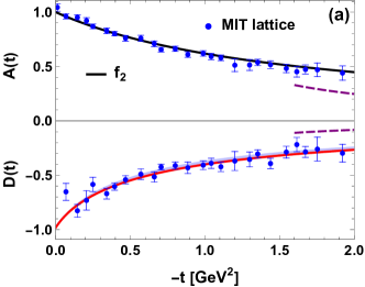
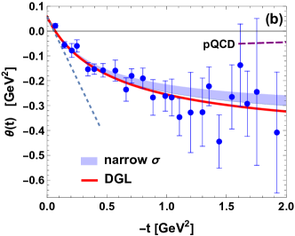
Figure 1: Gravitational form factors of the pion, plotted as functions of the space-like momentum transfer $-t$: (a) Form factors $A(t)$ and $D(t)$, with the data from [1]. The upper line (for $A$) is the monopole fit of Eq. (17) with the physical mass of $f_{2}(1270)$. The lower line (for $D$) is obtained from Eq. (5) and the model for $A$ and $\Theta(t)$. (b) The trace form factor $\Theta(t)$. The data are obtained from [1] via Eq. (5), with errors added in quadrature. The tangent (dashed line) at the origin is the $\chi$PT formula $2m_{\pi}^{2}+t$. The model curve (DGL) is obtained for the Donoghue, Gasser, and Leutwyler spectral density shown in Fig. 2, used in the dispersion relation (8). The long-dashed lines are the pQCD results for $\Lambda_{\rm QCD}=225~{}{\rm MeV}$ [29]. See the text for details.

Applying the standard resonance saturation by inserting a complete set of intermediate hadronic states yields

$$\langle\pi\pi|\Theta^{\mu\nu}|0\rangle=\sum_{R}\langle\pi\pi|R\rangle\frac{1}{m_{R}^{2}-q^{2}}\langle R|\Theta^{\mu\nu}|0\rangle,$$ (9)

with the contributions limited to $0^{++}$ and $2^{++}$ states. However, the field representation of higher spin particles, such as the tensor mesons, is not unique when particles are not on-shell and generally produces polynomial pieces which diverge at large energies. Instead, it is far more convenient to compute the absorptive part of the form factor which, which at $q^{2}\to s+i\epsilon$ reads

$$\frac{1}{\pi}{\rm Im}\langle\pi\pi|\Theta^{\mu\nu}|0\rangle=\sum_{R}\langle\pi\pi|R\rangle\langle R|\Theta^{\mu\nu}|0\rangle\delta(m_{R}^{2}-s),$$ (10)

and then reconstruct the dispersive part upon implementation of suitable subtraction constants. The vacuum to hadron transition amplitudes are

$$\langle S|\Theta^{\mu\nu}|0\rangle = f_{S}(g^{\mu\nu}q^{2}-q^{\mu}q^{\nu})/3,$$ (11)

$$\langle T|\Theta^{\mu\nu}|0\rangle = f_{T}m_{T}^{2}\epsilon^{\mu\nu}_{\lambda},$$

where $\epsilon^{\mu\nu}_{\lambda}$ is the spin-2 polarization tensor, which is symmetric $\epsilon^{\mu\nu}_{\lambda}=\epsilon^{\nu\mu}_{\lambda}$, traceless $g_{\mu\nu}\epsilon^{\mu\nu}_{\lambda}=0$, and transverse $q_{\mu}\epsilon^{\mu\nu}_{\lambda}=0$. The extra factor 3 in the definition is conventional such that $\langle S|\Theta|0\rangle=f_{S}m_{S}^{2}$. The on-shell couplings of the resonances to the $\pi\pi$ continuum are taken as

$$\langle S|\pi\pi\rangle = g_{S\pi\pi},$$ (12)

$$\langle T|\pi\pi\rangle = g_{T\pi\pi}\epsilon^{\alpha\beta}_{\lambda}P^{\alpha}P^{\beta}=g_{T\pi\pi}\epsilon^{\alpha\beta}_{\lambda}p^{\prime\alpha}p^{\beta}.$$

Thus, we get

$$\frac{1}{\pi}{\rm Im}\langle\pi\pi|\Theta^{\mu\nu}|0\rangle=\sum_{S}\frac{g_{S\pi\pi}f_{S}}{3}\delta(m_{S}^{2}-q^{2})(g^{\mu\nu}q^{2}-q^{\mu}q^{\nu})$$

$$+\sum_{T,\lambda}\epsilon_{\lambda}^{\alpha\beta}P^{\alpha}P^{\beta}\epsilon^{\mu\nu}_{\lambda}g_{T\pi\pi}f_{T}\delta(m_{T}^{2}-q^{2}),$$ (13)

which naturally complies with separate conservation for each contribution when contracting with $q^{\mu}$. The sum over tensor polarizations is given by [40, 41],

$$\sum_{\lambda}\epsilon_{\lambda}^{\alpha\beta}\epsilon^{\mu\nu}_{\lambda}=\frac{1}{2}\left(X^{\mu\alpha}X^{\nu\beta}+X^{\nu\alpha}X^{\mu\beta}\right)-\frac{1}{3}X^{\mu\nu}X^{\alpha\beta},$$ (14)

with $X^{\mu\nu}=g^{\mu\nu}-q^{\mu}q^{\nu}/q^{2}$, hence the on-shell condition $P\cdot q=0$ implies $P_{\alpha}X^{\alpha,\beta}=P^{\beta}$ and we get

$$\sum_{\lambda}\epsilon_{\lambda}^{\alpha\beta}P_{\alpha}P_{\beta}\epsilon^{\mu\nu}_{\lambda}=P^{\mu}P^{\nu}-\frac{1}{3}(g^{\mu\nu}-\frac{q^{\mu}q^{\nu}}{q^{2}})P^{2}$$ (15)

(cf. the tensor structure in Eq. (4)). Therefore, in the narrow resonance, large-$N_{c}$ motivated approach

$$\frac{1}{\pi}{\rm Im}A(s) = \frac{1}{2}\sum_{T}g_{T\pi\pi}f_{T}\delta(m_{T}^{2}-q^{2}),$$ (16)

$$\frac{1}{\pi}{\rm Im}\Theta(s) = \sum_{S}g_{S\pi\pi}f_{S}m_{S}^{2}\delta(m_{S}^{2}-q^{2}),$$

where, as expected, $A$ and $\Theta$ get contributions exclusively from the $2^{++}$ and $0^{++}$ states, respectively. As already suggested in [26], taking just one resonance per channel, i.e., using ${\rm Im}A(s)=\pi m_{f_{2}}^{2}\delta\left(s-m_{f_{2}}^{2}\right)$ and ${\rm Im}\Theta(s)=\pi m_{\sigma}^{4}\delta\left(s-m_{\sigma}^{2}\right)$ in the dispersion relations (6,8), gives

$$A(-Q^{2})=\frac{m_{f_{2}}^{2}}{m_{f_{2}}^{2}+Q^{2}},$$ (17)

$$\Theta(-Q^{2})=2m_{\pi}^{2}-\frac{m_{\sigma}^{2}Q^{2}}{m_{\sigma}^{2}+Q^{2}},$$ (18)

where the $2^{++}$ state is the $f_{2}(1270)$ meson, and the $0^{++}$ state is the $\sigma$ or $f_{0}(500)$ meson. The comparison of formula (17), taken with the Particle Data Group central value $m_{f_{2}}=1.275$ MeV, to the MIT lattice data [1] is shown in the top part of Fig. 1(a). As we can see, the data for $A$ are properly reproduced, with $\chi^{2}/{\rm DOF}=0.70$ for 25 data points, a success echoing the fit to the early noisy data [3, 4] in a similar model [13].

The scalar channel is more problematic since $\sigma$ is very broad and it is a priori not obvious what numerical value for $m_{\sigma}$ one should effectively use in the present context. Taking it as a model parameter, a fit to the lattice data for $D(t)$ obtained with Eq. (17,18) and relation (5) yields $m_{\sigma}=0.64(2)$ GeV, with $\chi^{2}/{\rm DOF}=0.97$ for 24 data points. The results for $D$ and $\Theta$ are shown in Fig. 1(a) and (b), respectively, with bands whose widths reflect the uncertainty in $m_{\sigma}$. The corresponding data points for $\Theta$ are obtained from the lattice data for $A$ and $D$ [1] with Eq. (2) (we have added the errors in quadrature, which may not be accurate due to possible correlations). We note a proper agreement of the model with the data.

Since $D$ depends on both the scalar and tensor channels, in an alternative strategy one can treat both $m_{f_{2}}$ and $m_{\sigma}$ as parameters in a joint fit to the $A$ and $D$ data. The result is $m_{f_{2}}=1.24(3)~{}{\rm GeV}$ and $m_{\sigma}=0.65(3)~{}{\rm GeV}$, with $\chi^{2}/{\rm DOF}=0.8$ for 49 data points. The corresponding model curves are very close to the previously described fit, hence are not displayed in the figure. We note that with the present lattice accuracy, any improvement of the model, such as adding higher states or nonzero widths with new fitted parameters, is not verifiable due to an appearance of overfitting. This feature is in fact consistent with the expected insensitivity of the space-like physics to the time-like details.

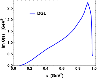
Figure 2: Digitized ${\rm Im}\,\Theta(s)$ from Fig. 3, case $A_{1}$, of [30]. Note that the spectral density incorporates the $\pi\pi$ rescattering, thus it has the physics of the $\sigma$ meson (a mild bump around $s\sim 0.4~{}{\rm GeV}$) and $f_{0}(980)$ (a minimum near its mass).

Given the fact that $f_{0}(500)$ is broad, it is worth to account for it in our analysis. In a more sophisticated treatment, we take ${\rm Im}\,\Theta(s)$ from the analysis of Donoghue, Gasser, and Leutwyler [30], where the physical scalar-isoscalar $\pi\pi$ phase shifts are used as input to solve the coupled $\pi\pi$ and $K\bar{K}$ channel Omnès-Muskhelishvili equations [42], with constants fixed by $\chi$PT. For definiteness, we use case $A_{1}$ from Fig. 3 of [30], corresponding to a solution with the CERN-Cracow-Munich [43] phase shifts as input. The used digitized ${\rm Im}\,\Theta(s)$ is shown in Fig. 2. The upper limit is about $\lambda^{2}\sim 1{\rm~{}GeV}^{2}$, the vicinity of $f_{0}(980)$, where ${\rm Im}\,\Theta(s)$ sharply drops to a low value. Then, we use dispersion relation (8), integrating up to $\lambda^{2}$ to obtain $\Theta(-Q^{2})$ in the space-like region. Since the MIT lattice data are for $m_{\pi}=170$ MeV, whereas the physical analysis is of course at the physical value of $m_{\pi}$, we take in Eq. (8) the lattice value in the $2m_{\pi}^{2}$ term.

We see some remarkable features in Fig. 1(b). The lowest $Q^{2}=-t$ data point is above zero at the $2.5\sigma$ level, in accordance with the positivity of $\Theta(0)=2m_{\pi}^{2}$. The model slope at the origin is

$$\left.d\Theta(t)/dt\right|_{t=0}=\frac{1}{\pi}\int_{4m_{\pi}^{2}}^{\lambda^{2}}ds\frac{{\rm Im}\Theta(s)}{s^{2}}\simeq 1,$$ (19)

close to the chiral limit value, which is indicated with the dashed line in Fig. 1(b), showing $2m_{\pi}^{2}+t$. We note that the model follows the data within the uncertainties. At larger values of $Q^{2}$ the errors are too large to draw strong conclusions, yet in the covered range the data seem to flatten. At large $Q^{2}$, the dispersion relation (8) with the literally taken spectral function of Fig. 2 and the upper limit $\lambda^{2}$ yields

$$\Theta(-Q^{2})\sim 2m_{\pi}^{2}-\int_{4m_{\pi}^{2}}^{\lambda^{2}}\!\!\!ds\,{\rm Im}\Theta(s)/s\simeq-0.46~{}{\rm GeV}^{2}.$$ (20)

We will return to the issue of the asymptotics shortly.

At the origin,

$$D(0)=-1+\frac{4m_{\pi}^{2}}{3m_{f_{2}}^{2}}-\frac{2}{3}\left[\left.d\Theta(t)/dt\right|_{t=0}-1\right]$$

$$\hskip 56.9055pt=-1+{\cal O}(m_{\pi}^{2})\simeq-0.98.$$ (21)

The gravitational ms (mean squared) radii, defined as $\langle r^{2}\rangle_{F}=\left.6(dF(t)/dt)/F(t)\right|_{t=0}$, are

$$\langle r^{2}\rangle_{A}=\frac{6}{m_{f_{2}}^{2}}=(0.38~{}{\rm fm})^{2},$$ (22)

$$\langle r^{2}\rangle_{D}=\frac{1}{D(0)}\left[-\frac{2}{m_{f_{2}}^{2}}-\frac{4}{\pi}\int_{4m_{\pi}^{2}}^{\lambda^{2}}ds\frac{{\rm Im}\Theta(s)}{s^{3}}+\frac{8m_{\pi}^{2}}{m_{f_{2}}^{4}}\right]$$

$$\hskip 56.9055pt\simeq(0.71~{}{\rm fm})^{2}.$$

The obtained numbers and the hierarchy pattern $\langle r^{2}\rangle_{A}<\langle r^{2}\rangle_{EM}<\langle r^{2}\rangle_{D}$ (where $\langle r^{2}\rangle_{EM}=(0.659(4)~{}{\rm fm})^{2}$ is the electromagnetic ms radius of the pion) are consistent with the analysis of [21] for the quark radii (our value for $\langle r^{2}\rangle_{D}$ is 20% smaller). With the narrow $\sigma$ discussed earlier, we get $D(0)=-1+4m_{\pi}^{2}/(3m_{f_{2}}^{2})=-0.98$ and

$$\langle r^{2}\rangle_{D}=\frac{1}{D(0)}\left[-\frac{2}{m_{f_{2}}^{2}}-\frac{4}{m_{\sigma}^{2}}+\frac{8m_{\pi}^{2}}{m_{f_{2}}^{4}}\right]\simeq(0.66~{}{\rm fm})^{2}.$$ (23)

In the chiral limit, sum rule (20) with a positive spectral function means that the large-$Q^{2}$ value of $\Theta$ is negative. Given the smallness of $\Theta(0)=2m_{\pi}^{2}$ and the slope equal to 1, one expects a zero at $t=-Q_{0}^{2}$, i.e., $\Theta(-Q_{0}^{2})=0$, where at LO in the chiral expansion $Q_{0}^{2}=2m_{\pi}^{2}$. This behavior is indeed seen in Fig. 1(b), where the change of sign occurs at $Q_{0}^{2}\simeq 0.07~{}{\rm GeV}^{2}$, slightly above the value $2m_{\pi}^{2}$.

At NLO $\chi$PT, the spectral function above the $2\pi$ production threshold is [30]

$$\frac{1}{\pi}{\rm Im}\Theta(s)=\frac{\sqrt{1-\frac{4m_{\pi}^{2}}{s}}\left(2m_{\pi}^{2}+s\right)\left(2s-m_{\pi}^{2}\right)}{32\pi^{2}f_{\pi}^{2}},$$ (24)

which is manifestly positive. Assuming, for the sake of an estimate, $\Lambda_{\chi}=4m_{\pi}^{2}$, corresponding to the $4\pi$ production threshold, one obtains the contribution to the mass sum rule (20)

$$-\frac{1}{\pi}\int_{4m_{\pi}^{2}}^{16m_{\pi}^{2}}ds\frac{{\rm Im}\Theta(s)}{s}=-0.03~{}{\rm GeV}^{2},$$ (25)

which is about $50\%$ of the value at the origin, $\Theta(0)=2m_{\pi}^{2}$, and small compared to the values reached in Fig. 1(b) at higher $Q^{2}$.

To analyze the high energy limit, we recall that the trace anomaly of QCD reads

$$\Theta^{\mu}_{\mu}=\frac{\beta(\alpha)}{4\alpha}{G^{\mu\nu}}^{2}+[1+\gamma_{m}(\alpha)]\sum_{f}m_{f}\bar{q}_{f}q_{f},$$ (26)

where $f$ enumerates active flavors, $\beta(\alpha)=\mu^{2}d\alpha/d\mu^{2}=-\alpha[\beta_{0}(\alpha/4\pi)+\dots]<0$ is the QCD beta function, $\gamma_{m}(\alpha)=2\alpha/\pi+\dots$ is the quark mass anomalous dimension, $\alpha(-Q^{2})=(4\pi/\beta_{0})\ln\left(Q^{2}/\Lambda_{\rm QCD}^{2}\right)$ is the running strong coupling constant, and $\beta_{0}=\tfrac{1}{3}(11N_{c}-2N_{f})$, with $N_{c}=3$ colors and $N_{f}$ active flavors. Interesting conclusions for the spectral density may be drawn from the recently obtained asymptotic behavior of the components of $\Theta(Q^{2})$. The quark contribution yields about 25% to the normalization at $Q^{2}=0$ [46, 47] and in pQCD, the behavior of the scalar-isoscalar form factor related to the chirally odd quark component of (26) can be written as $m_{q}\langle\pi(p^{\prime})|\bar{q}q(0)|\pi(p)\rangle\sim c\,m_{\pi}^{2}f_{\pi}^{2}\alpha(-Q^{2})/Q^{2}$ [48], with a constant $c$. The situation is different, however, for the gluonic part, where it has recently been shown [29] that at $Q^{2}\to\infty$

$$\langle\pi(p^{\prime})|\frac{\beta(\alpha)}{4\alpha}{G^{\mu\nu}}^{2}(0)|\pi(p)\rangle\sim 16\pi\beta\left(\alpha(-Q^{2})\right)f_{\pi}^{2},$$ (27)

which means that $\Theta(-Q^{2})$ goes to zero from the negative side very slowly, as a negative constant divided by $(\ln Q^{2}/\Lambda_{\rm QCD}^{2})^{2}$ (see the long-dashed line in Fig. 1(b)). This flatness is also quite spectacularly seen in the lattice simulations of the gluonic trace anomaly [7], which extend to $Q^{2}\sim 3.7~{}{\rm GeV}^{2}$ (albeit with pion masses significantly higher from the physical value).

Dispersion relation (8) leads to the sum rule

$$2m_{\pi}^{2}-\frac{1}{\pi}\int_{4m_{\pi}^{2}}^{\infty}ds\frac{{\rm Im}\,\Theta(s)}{s}=0.$$ (28)

In view of the earlier discussion, where the integration with the spectral density of Fig. 2 up to $\lambda^{2}\sim 1~{}{\rm GeV}^{2}$ led to a large negative value of $\Theta(-Q^{2})$, sum rule (28) means that ${\rm Im}\Theta(s)$ cannot be positive definite and needs to acquire a negative sign at larger values of $s$, beyond the range shown in Fig. 2. We remark that positivity of a three-point spectral function is not formally protected.

Actually, the dispersive integral can be evaluated upwards from a high mass scale $\Lambda$, where pQCD is supposed to set in, by analytically continuing the LO pQCD result from negative space-like region $t=-Q^{2}$ to the complex plane $-t=e^{-i\theta}|t|$. Thus, the positive time-like region corresponds to $\theta\to-\pi$, such that one has $q^{2}=s+i\epsilon$ and $\ln(Q^{2}/\Lambda^{2})\to\ln(se^{-i\pi}/\Lambda^{2})=\ln(s/\Lambda^{2})-i\pi$. On the upper lip of the cut at $s\gg 4m_{\pi}^{2}$, with the notation $L=\log(s/\Lambda_{\rm QCD}^{2})$, one gets

$$\alpha(s)\equiv\alpha(s+i\epsilon)=\left(\frac{4\pi}{\beta_{0}}\right)\frac{1}{L-i\pi},$$ (29)

yielding a positive imaginary part ${\rm Im}\,\alpha(s+i\epsilon)^{2}=(4\pi/\beta_{0})^{2}2\pi L/(L^{2}+\pi^{2})^{2}$, hence

$$\frac{1}{\pi}{\rm Im}\Theta(s)=-\left(\frac{4\pi}{\beta_{0}}\right)^{2}\frac{4\beta_{0}Lf_{\pi}^{2}}{(L^{2}+\pi^{2})^{2}}+{\cal O}(\alpha^{3}).$$ (30)

This implies that ${\rm Im}\Theta(s)<0$ at large energies, which is the desired result. After computing the integral, the contribution to sum rule (28) is

$$-\frac{1}{\pi}\int_{\Lambda^{2}}^{\infty}ds\frac{{\rm Im}\Theta(s)}{s}=4\beta_{0}[\alpha(-\Lambda^{2})]^{2}f_{\pi}^{2}+{\cal O}(\alpha^{3}),$$ (31)

which for $\Lambda^{2}\sim 20\Lambda_{\rm QCD}^{2}\sim 1{\rm GeV}^{2}$ is about $5f_{\pi}^{2}\sim 0.04~{}{\rm GeV}^{2}$, small compared to the values reached in Fig. 1. This means that the spectral function must acquire negative values at lower values of $s$ than $\Lambda^{2}$, and/or pick them up from higher order or non-perturbative effects.

The asymptotic values of $A(-Q^{2})$ and $D(-Q^{2})$ vanish as $1/Q^{2}$ divided by log corrections [28, 29, 51]. Therefore the following sum rules immediately follow:

$$0 = 1-\frac{1}{\pi}\int_{4m_{\pi}^{2}}^{\infty}ds\frac{1}{s}{\rm Im}\,A(s),$$

$$0 = D(0)-\frac{1}{\pi}\int_{4m_{\pi}^{2}}^{\infty}ds\frac{1}{s}{\rm Im}\,D(s).$$ (32)

In fact, since $Q^{2}A(-Q^{2})$ and $Q^{2}D(Q^{2})$ also tend to zero due to the extra suppression by $1/\ln Q^{2}$ from $\alpha$, one has two more sum rules:

$$0=\frac{1}{\pi}\int_{4m_{\pi}^{2}}^{\infty}ds\,{\rm Im}A(s),\;\;\;\;0=\frac{1}{\pi}\int_{4m_{\pi}^{2}}^{\infty}ds\,{\rm Im}D(s),$$ (33)

implying that the spectral densities for $A(s)$ and $D(s)$ cannot have a well-defined sign.

In conclusion, we have shown that the high precision MIT lattice QCD data for the gravitational form factors of the pion can be naturally understood and accurately described with the meson dominance principle, working very well in the momentum transfer range used on the lattice. The analysis requires the projection on good spin quantum numbers. The tensor $2^{++}$ component, corresponding to $A$, can be saturated with the $f_{2}(1270)$ meson whereas the scalar $0^{++}$ component (the trace form factor $\Theta$) can be described by using the physical spectral function (involving the scalar-isoscalar $\sigma$ meson) in the dispersion relation. The form factor $D$ is obtained as a combination of $A$ and $\Theta$. We have also exploited the pQCD constraints at high momentum transfers, with the peculiar feature that at infinite space-like momentum $\Theta(-Q^{2})$ goes to a constant times log corrections. These constraints lead to sum rules for the spectral densities of the gravitational form factors, which imply that these densities cannot be of definite sign. The numerical smallness of the (negative) LO pQCD contribution to the spectral density of $\Theta$, together with a positive contribution from $\chi$PT and a large positive contribution from the resonance region up to $s\sim 1~{}{\rm GeV}^{2}$, means that the higher mass resonances or higher orders in pQCD must bring in large negative contributions to the spectral density of $\Theta$. This feature is needed to reconcile the available lattice data and the theoretical requirements.

We are grateful to the authors of Ref. [1] for providing us the data tables for Fig. 1(a), as well as to the authors of Ref. [7] for communicating their numerical results. Supported by the Polish National Science Centre grant 2018/31/B/ST2/01022 (WB), by the Spanish MINECO and European FEDER funds grant and Project No. PID2020–114767 GB-I00 funded by MCIN/AEI/10.13039/501100011033, and by the Junta de Andalucía grant FQM-225 (ERA).

References

- Hackett et al. [2023] D. C. Hackett, P. R. Oare, D. A. Pefkou, P. E. Shanahan, Gravitational form factors of the pion from lattice QCD, Phys. Rev. D 108 (2023) 114504. doi:10.1103/PhysRevD.108.114504. arXiv:2307.11707.
- Pefkou [2023] D. A. Pefkou, Gravitational form factors of hadrons from lattice QCD, Ph.D. thesis, MIT, 2023.
- Brommel [2007] D. Brommel, Pion Structure from the Lattice, Ph.D. thesis, Regensburg U., 2007. doi:10.3204/DESY-THESIS-2007-023.
- Brömmel et al. [2008] D. Brömmel, et al. (QCDSF, UKQCD), The Spin structure of the pion, Phys. Rev. Lett. 101 (2008) 122001. doi:10.1103/PhysRevLett.101.122001. arXiv:0708.2249.
- Delmar et al. [2024] J. Delmar, C. Alexandrou, S. Bacchio, I. Cloët, M. Constantinou, G. Koutsou, Generalized form factors of the pion and kaon using twisted mass fermions, in: 40th International Symposium on Lattice Field Theory, 2024. arXiv:2401.04080.
- Shanahan and Detmold [2019] P. E. Shanahan, W. Detmold, Gluon gravitational form factors of the nucleon and the pion from lattice QCD, Phys. Rev. D 99 (2019) 014511. doi:10.1103/PhysRevD.99.014511. arXiv:1810.04626.
- Wang et al. [2024] B. Wang, F. He, G. Wang, T. Draper, J. Liang, K.-F. Liu, Y.-B. Yang (QCD), Trace anomaly form factors from lattice QCD, Phys. Rev. D 109 (2024) 094504. doi:10.1103/PhysRevD.109.094504. arXiv:2401.05496.
- Pagels [1966] H. Pagels, Energy-momentum structure form factors of particles, Phys. Rev. 144 (1966) 1250–1260. doi:10.1103/PhysRev.144.1250.
- Polyakov and Schweitzer [2018] M. V. Polyakov, P. Schweitzer, Forces inside hadrons: pressure, surface tension, mechanical radius, and all that, Int. J. Mod. Phys. A 33 (2018) 1830025. doi:10.1142/S0217751X18300259. arXiv:1805.06596.
- Broniowski et al. [2008] W. Broniowski, E. Ruiz Arriola, K. Golec-Biernat, Generalized parton distributions of the pion in chiral quark models and their QCD evolution, Phys. Rev. D 77 (2008) 034023. doi:10.1103/PhysRevD.77.034023. arXiv:0712.1012.
- Broniowski and Ruiz Arriola [2008] W. Broniowski, E. Ruiz Arriola, Gravitational and higher-order form factors of the pion in chiral quark models, Phys. Rev. D 78 (2008) 094011. doi:10.1103/PhysRevD.78.094011. arXiv:0809.1744.
- Frederico et al. [2009] T. Frederico, E. Pace, B. Pasquini, G. Salme, Pion Generalized Parton Distributions with covariant and Light-front constituent quark models, Phys. Rev. D 80 (2009) 054021. doi:10.1103/PhysRevD.80.054021. arXiv:0907.5566.
- Masjuan et al. [2013] P. Masjuan, E. Ruiz Arriola, W. Broniowski, Meson dominance of hadron form factors and large- phenomenology, Phys. Rev. D 87 (2013) 014005. doi:10.1103/PhysRevD.87.014005. arXiv:1210.0760.
- Fanelli et al. [2016] C. Fanelli, E. Pace, G. Romanelli, G. Salme, M. Salmistraro, Pion Generalized Parton Distributions within a fully covariant constituent quark model, Eur. Phys. J. C 76 (2016) 253. doi:10.1140/epjc/s10052-016-4101-1. arXiv:1603.04598.
- Freese and Cloët [2019] A. Freese, I. C. Cloët, Gravitational form factors of light mesons, Phys. Rev. C 100 (2019) 015201. doi:10.1103/PhysRevC.100.015201. arXiv:1903.09222, [Erratum: Phys.Rev.C 105, 059901 (2022)].
- Krutov and Troitsky [2021] A. F. Krutov, V. E. Troitsky, Pion gravitational form factors in a relativistic theory of composite particles, Phys. Rev. D 103 (2021) 014029. doi:10.1103/PhysRevD.103.014029. arXiv:2010.11640.
- Xing et al. [2023] Z. Xing, M. Ding, L. Chang, Glimpse into the pion gravitational form factor, Phys. Rev. D 107 (2023) L031502. doi:10.1103/PhysRevD.107.L031502. arXiv:2211.06635.
- Xu et al. [2024] Y.-Z. Xu, M. Ding, K. Raya, C. D. Roberts, J. Rodríguez-Quintero, S. M. Schmidt, Pion and kaon electromagnetic and gravitational form factors, Eur. Phys. J. C 84 (2024) 191. doi:10.1140/epjc/s10052-024-12518-x. arXiv:2311.14832.
- Li and Vary [2024] Y. Li, J. P. Vary, Stress inside the pion in holographic light-front QCD, Phys. Rev. D 109 (2024) L051501. doi:10.1103/PhysRevD.109.L051501. arXiv:2312.02543.
- Masuda et al. [2016] M. Masuda, et al. (Belle), Study of pair production in single-tag two-photon collisions, Phys. Rev. D 93 (2016) 032003. doi:10.1103/PhysRevD.93.032003. arXiv:1508.06757.
- Kumano et al. [2018] S. Kumano, Q.-T. Song, O. V. Teryaev, Hadron tomography by generalized distribution amplitudes in pion-pair production process and gravitational form factors for pion, Phys. Rev. D 97 (2018) 014020. doi:10.1103/PhysRevD.97.014020. arXiv:1711.08088.
- Ji [1995] X.-D. Ji, A QCD analysis of the mass structure of the nucleon, Phys. Rev. Lett. 74 (1995) 1071–1074. doi:10.1103/PhysRevLett.74.1071. arXiv:hep-ph/9410274.
- Lorcé [2018] C. Lorcé, On the hadron mass decomposition, Eur. Phys. J. C 78 (2018) 120. doi:10.1140/epjc/s10052-018-5561-2. arXiv:1706.05853.
- Hatta et al. [2018] Y. Hatta, A. Rajan, K. Tanaka, Quark and gluon contributions to the QCD trace anomaly, JHEP 12 (2018) 008. doi:10.1007/JHEP12(2018)008. arXiv:1810.05116.
- Novikov and Shifman [1981] V. A. Novikov, M. A. Shifman, Comment on the psi-prime — J/psi pi pi Decay, Z. Phys. C 8 (1981) 43. doi:10.1007/BF01429829.
- Donoghue and Leutwyler [1991] J. F. Donoghue, H. Leutwyler, Energy and momentum in chiral theories, Z. Phys. C 52 (1991) 343–351. doi:10.1007/BF01560453.
- Raman [1971] K. Raman, Gravitational form-factors of pseudoscalar mesons, stress-tensor-current commutation relations, and deviations from tensor- and scalar-meson dominance, Phys. Rev. D 4 (1971) 476–488. doi:10.1103/PhysRevD.4.476.
- Tong et al. [2021] X.-B. Tong, J.-P. Ma, F. Yuan, Gluon gravitational form factors at large momentum transfer, Phys. Lett. B 823 (2021) 136751. doi:10.1016/j.physletb.2021.136751. arXiv:2101.02395.
- Tong et al. [2022] X.-B. Tong, J.-P. Ma, F. Yuan, Perturbative calculations of gravitational form factors at large momentum transfer, JHEP 10 (2022) 046. doi:10.1007/JHEP10(2022)046. arXiv:2203.13493.
- Donoghue et al. [1990] J. F. Donoghue, J. Gasser, H. Leutwyler, The Decay of a Light Higgs Boson, Nucl. Phys. B 343 (1990) 341–368. doi:10.1016/0550-3213(90)90474-R.
- Nieves and Ruiz Arriola [2000] J. Nieves, E. Ruiz Arriola, Bethe-Salpeter approach for unitarized chiral perturbation theory, Nucl. Phys. A 679 (2000) 57–117. doi:10.1016/S0375-9474(00)00321-3. arXiv:hep-ph/9907469.
- Nieves and Ruiz Arriola [2009] J. Nieves, E. Ruiz Arriola, Meson Resonances at large Nc: Complex Poles vs Breit- Wigner Masses, Phys. Lett. B679 (2009) 449–453. doi:10.1016/j.physletb.2009.08.021. arXiv:0904.4590 [hep-ph].
- Ecker et al. [1989a] G. Ecker, J. Gasser, H. Leutwyler, A. Pich, E. de Rafael, Chiral lagrangians for massive spin 1 fields, Phys. Lett. B223 (1989a) 425.
- Ecker et al. [1989b] G. Ecker, J. Gasser, A. Pich, E. de Rafael, The role of resonances in chiral perturbation theory, Nucl. Phys. B321 (1989b) 311.
- Pich [2002] A. Pich, Colorless mesons in a polychromatic world, in: The Phenomenology of Large QCD, 2002, pp. 239–258. doi:10.1142/9789812776914\_0023. arXiv:hep-ph/0205030.
- Ledwig et al. [2014] T. Ledwig, J. Nieves, A. Pich, E. Ruiz Arriola, J. Ruiz de Elvira, Large- naturalness in coupled-channel meson-meson scattering, Phys. Rev. D 90 (2014) 114020. doi:10.1103/PhysRevD.90.114020. arXiv:1407.3750.
- Toublan [1996] D. Toublan, Lowest tensor meson resonances contributions to the chiral perturbation theory low-energy coupling constants, Phys. Rev. D 53 (1996) 6602–6607. doi:10.1103/PhysRevD.53.6602. arXiv:hep-ph/9509217, [Erratum: Phys.Rev.D 57, 4495 (1998)].
- Ecker and Zauner [2007] G. Ecker, C. Zauner, Tensor meson exchange at low energies, Eur. Phys. J. C 52 (2007) 315–323. doi:10.1140/epjc/s10052-007-0372-x. arXiv:0705.0624.
- Nieves et al. [2011] J. Nieves, A. Pich, E. Ruiz Arriola, Large-Nc Properties of the rho and f0(600) Mesons from Unitary Resonance Chiral Dynamics, Phys. Rev. D 84 (2011) 096002. doi:10.1103/PhysRevD.84.096002. arXiv:1107.3247.
- Scadron [1968] M. D. Scadron, Covariant Propagators and Vertex Functions for Any Spin, Phys. Rev. 165 (1968) 1640–1647. doi:10.1103/PhysRev.165.1640.
- Novozhilov [1975] Y. V. Novozhilov, Introduction to Elementary Particle Theory, International Series of Monographs In Natural Philosophy, Pergamon Press, Oxford, UK, 1975.
- Pham and Truong [1977] T. N. Pham, T. N. Truong, Muskhelishvili-Omnes Integral Equation with Inelastic Unitarity: Single and Coupled Channel Equations, Phys. Rev. D 16 (1977) 896. doi:10.1103/PhysRevD.16.896.
- Becker et al. [1979] H. Becker, G. Blanar, W. Blum, M. Cerrada, H. Dietl, J. Gallivan, B. Gottschalk, G. Grayer, G. Hentschel, E. Lorenz, et al., A model-independent partial-wave analysis of the -system produced at low four-momentum transfer in the reaction at 17.2 GeV/c, Nucl. Phys. B 151 (1979) 46–70.
- Ananthanarayan et al. [2001] B. Ananthanarayan, G. Colangelo, J. Gasser, H. Leutwyler, Roy equation analysis of pi pi scattering, Phys. Rept. 353 (2001) 207–279. doi:10.1016/S0370-1573(01)00009-6. arXiv:hep-ph/0005297.
- Garcia-Martin et al. [2011] R. Garcia-Martin, R. Kaminski, J. R. Pelaez, J. Ruiz de Elvira, F. J. Yndurain, The Pion-pion scattering amplitude. IV: Improved analysis with once subtracted Roy-like equations up to 1100 MeV, Phys. Rev. D 83 (2011) 074004. doi:10.1103/PhysRevD.83.074004. arXiv:1102.2183.
- Gasser and Leutwyler [1982] J. Gasser, H. Leutwyler, Quark Masses, Phys. Rept. 87 (1982) 77–169. doi:10.1016/0370-1573(82)90035-7.
- Ji [1995] X.-D. Ji, Breakup of hadron masses and energy - momentum tensor of QCD, Phys. Rev. D 52 (1995) 271–281. doi:10.1103/PhysRevD.52.271. arXiv:hep-ph/9502213.
- Lepage and Brodsky [1980] G. P. Lepage, S. J. Brodsky, Exclusive Processes in Perturbative Quantum Chromodynamics, Phys. Rev. D 22 (1980) 2157. doi:10.1103/PhysRevD.22.2157.
- Donoghue and Na [1997] J. F. Donoghue, E. S. Na, Asymptotic limits and structure of the pion form-factor, Phys. Rev. D 56 (1997) 7073–7076. doi:10.1103/PhysRevD.56.7073. arXiv:hep-ph/9611418.
- Ruiz Arriola and Sanchez-Puertas [2024] E. Ruiz Arriola, P. Sanchez-Puertas, The phase of the electromagnetic form factor of the pion (2024). arXiv:2403.07121.
- Krutov and Troitsky [2023] A. F. Krutov, V. E. Troitsky, Pion gravitational form factors at large momentum transfer in the instant-form relativistic impulse approximation approach, Phys. Rev. D 108 (2023) 094043. doi:10.1103/PhysRevD.108.094043. arXiv:2310.14287.