On the quadratic stability of asymmetric Hermite basis and application to plasma physics

Abstract

We analyze why the discretization of linear transport with asymmetric Hermite basis functions can be instable in quadratic norm. The main reason is that the finite truncation of the infinite moment linear system looses the skew-symmetry property with respect to the Gram matrix. Then we propose an original closed formula for the scalar product of any pair of asymmetric basis functions. It makes possible the construction of two simple modifications of the linear systems which recover the skew-symmetry property. By construction the new methods are quadratically stable with respect to the natural $L^{2}$ norm. We explain how to generalize to other transport equations encountered in numerical plasma physics. Basic numerical tests illustrate the unconditional stability properties of our algorithms.

1 Introduction

Asymmetric Hermite basis are widely used for the numerical discretization of transport phenomenon in plasma physics, since they are amenable for the preservation of natural invariants such as the total mass or the total energy. However they are not symmetric which, on mathematical grounds, means that they do not constitute an orthonormal family of the space $L^{2}(\mathbb{R})$ endowed with the scalar product

$$(\alpha,\beta)=\int_{\mathbb{R}}\alpha(v)\beta(v)dv,\qquad\alpha,\beta\in L^{2}(\mathbb{R}).$$ (1)

In consequence they can trigger numerical instabilities in numerical methods. The aim of our work is to explain how to recover the hidden quadratic stability of asymmetric Hermite basis, which turns into new and stable numerical methods. Mathematically this is based on exact formulas for the calculation of the scalar product of two asymmetric functions. To the best of our knowledge, these formulas are original with respect to the huge literature on special functions [16, 12].

In plasma physics literature [1, 7, 8, 9, 11, 17, 10, 13, 18, 4], the theory of Hermite basis is often motivated by the development of plasma numerical simulators. The convergence of the Hermite-Fourier method with symmetric functions is provided in [13, 6, 3]: unfortunately the theory is difficult to extend to the asymmetric case. The seminal reference is Holloway who discussed these two cases in [8]. When employing symmetrically-weighted basis functions, particle number, mass and total energy are preserved for odd number of moments, or momentum are preserved for even number of moments. On the other hand, asymmetrically-weighted basis functions, conserves particle number, total energy and momentum simultaneously. In [10], K. Kormann and A. Yurova, using the idea of telescoping sums to show conservation for the symmetrically-weighted and asymmetrically-weighted cases, reached conclusions consistent with those in [8]. This is the reason why researchers are more interested in asymmetrically-weighted basis functions.

Subsequent research [18] by Schumer and Holloway conducted comprehensive numerical simulations of both symmetric and asymmetric methods, revealing that the asymmetrically-weighted Hermite method became numerically unstable. On the contrary, the symmetrically-weighted method is more robust and suitable for long-time simulations. Among recent works which explicitly mention the instability of asymmetric basis, we quote [13, 2] where the first contribution relies on adding a Fokker-Planck perturbation to enforce stability while the second contribution details a weighted norm which changes dynamically in time (its net effect is that the underlying reference temperature increases in time). Funaro and Manzini provide in [6] a mathematical investigation of the stability of the Hermite-Fourier spectral approximation of the Vlasov-Poisson model for a collisionless plasma in the electrostatic limit. The analysis includes high-order artificial collision operators of Lenard-Bernstein type. In [15], the authors proposed a spectral method for the 1D-1V Vlasov-Poisson system where the discretization in velocity space is based on asymmetrically-weighted Hermite functions, dynamically adapted through two velocity variables, which aims to maintain the stability of the numerical solution. To our knowledge, none of the quoted works has ever explained the origin of the numerical instability of asymmetric basis.

Our theoretical contributions are threefold. Firstly we provide a simple linear explanation of the numerical instability phenomenon. Secondly we propose in Theorems 4.1 and 4.4 original compact formulas for the scalar product (1) of two asymmetric Hermite functions. Thirdly we show how to modify the matrices of the discrete problem so as to recover the natural stability of the model problem, as in Lemma 5.1 for example.

The plan of this work is as follows. In Section 2, we provide a simple example of the instability attached to truncated asymmetric basis for the numerical simulation of $\partial_{t}f+e\partial_{v}f=0$. Then in Section 3, we analyze the structure of the Gram matrix of asymmetric basis. Section 4 is devoted to the exact calculation of the coefficients of the Gram matrix, where we propose formulas which are new to our knowledge. In Section 5 we present two easy-to-implement modifications of the matrix of the problem, where the antisymmetry with respect to the Gram matrix is recovered by construction. The next Section 6 is devoted to a simple generalization to the equation $\partial_{t}f+v\partial_{x}f=0$. Finally, Section 7, we illustrate the general properties with numerical tests.

The notations try to keep the technicalities to the minimum, and we will use the language of linear algebra to detail the properties of the various objects.

2 Notations and illustration of the numerical instability

Our model problem is the transport equation in velocity

$$\partial_{t}f(t,v)+e\partial_{v}f(t,v)=0.$$ (2)

The constant $e>0$ represents some constant electric field (for plasma physics applications). Any solution of the equation preserves the quadratic norm

$$\frac{d}{dt}\int_{\mathbb{R}}f(t,v)^{2}dv=0.$$ (3)

Let $(H_{m})_{m\in\mathbb{N}}$ be the family of Hermite polynomials [16, 19, 12] which is orthogonal with respect to the Gaussian weight $e^{-v^{2}}$. Introducing a reference temperature $T>0$ (for plasma physics applications), the asymmetric basis $(\psi_{m})_{m\in\mathbb{N}}$ and the asymmetric basis $(\psi^{m})_{m\in\mathbb{N}}$ are defined as

$$\left\{\begin{array}[]{lrl}\psi_{m}(v)=&e^{\frac{-v^{2}}{T}}T^{-\frac{1}{2}}(2^{m}m!\sqrt{\pi})^{-\frac{1}{2}}H_{m}(v/\sqrt{T}),\\ \psi^{m}(v)=&(2^{m}m!\sqrt{\pi})^{-\frac{1}{2}}H_{m}(v/\sqrt{T})&=e^{\frac{v^{2}}{T}}T^{\frac{1}{2}}\psi_{m}(v).\end{array}\right.$$

Due to orthogonality property $\int_{\mathbb{R}}\psi_{m}(v)\psi^{n}(v)dv=\delta_{mn}$, the two families are dual. The classical symmetric Hermite function corresponds to

$$\phi_{m}(v)=e^{\frac{v^{2}}{2T}}T^{\frac{1}{4}}\psi_{m}(v)=e^{\frac{-v^{2}}{2T}}T^{-\frac{1}{4}}\psi^{m}(v).$$

The family of Hermite functions $(\phi_{m})_{m\in\mathbb{N}}$ forms a complete orthonormal family (Hilbertian family) of $L^{2}(\mathbb{R})$. Other important identities for all $m\in\mathbb{N}$ are

$$(\psi_{m})^{\prime}(v)=-\sqrt{\frac{2(m+1)}{T}}\ \psi_{m+1}(v)\mbox{ and }(\psi^{m})^{\prime}(v)=\sqrt{\frac{2m}{T}}\ \psi^{m-1}(v).$$

The second identity is natural because the derivative of a polynomial is a polynomial of lesser degree. The first property can be deduced with the help of duality between $(\psi_{m})_{m\in\mathbb{N}}$ and $(\psi^{m})_{m\in\mathbb{N}}$.

Then the common procedure to discretize (2) starts from the a priori infinite representation

$$f(v)=\sum_{m\geq 0}u_{m}\psi_{m}\left(v\right)$$ (4)

where the coefficients $u_{m}$ are the moments of the function $f$. By definition one has

$$e^{\frac{v^{2}}{2T}}T^{\frac{1}{4}}f(v)=\sum_{m\geq 0}u_{m}\phi_{m}\left(v\right).$$ (5)

The condition for the convergence in $L^{2}(\mathbb{R})$ of the series in (5) writes as

$$e^{\frac{v^{2}}{2T}}T^{\frac{1}{4}}f\in L^{2}(\mathbb{R})\Longleftrightarrow\left\|e^{\frac{v^{2}}{2T}}T^{\frac{1}{4}}f\right\|_{L^{2}(\mathbb{R})}^{2}=\sum_{m\geq 0}|u_{m}|^{2}<\infty.$$ (6)

Let $f(v,t)$ be a solution of the transport equation (2). Under convenient convergence conditions on the series, one has

$$\left\{\begin{array}[]{lll}\partial_{t}f(t,v)=\sum_{m\geq 0}u_{m}^{\prime}(t)\psi_{m}\left(v\right),\\ \partial_{v}f(t,v)=-\sum_{m\geq 0}u_{m}(t)\sqrt{\frac{2(m+1)}{T}}\psi_{m+1}\left(v\right).\end{array}\right.$$

Therefore (2) rewrites as

$$\sum_{m\geq 0}u_{m}^{\prime}(t)\psi_{m}\left(v\right)-e\sum_{m\geq 0}u_{m}(t)\sqrt{\frac{2(m+1)}{T}}\psi_{m+1}\left(v\right)=0$$

from which one deduces the identities

$$u_{0}^{\prime}(t)=0\mbox{ and }u_{m}^{\prime}(t)-e\sqrt{\frac{2m}{T}}u_{m-1}(t)=0\mbox{ for all }m\geq 1.$$ (7)

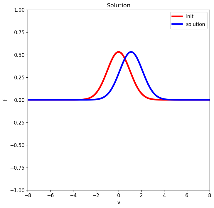
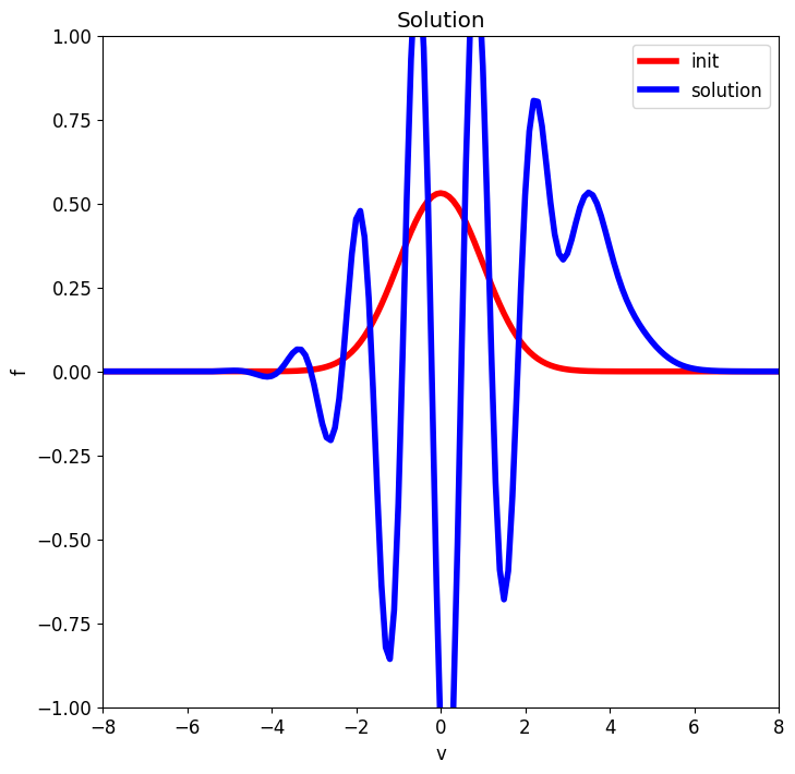
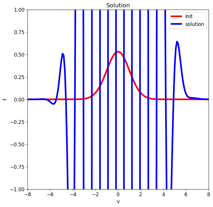
Figure 1: Results of the advection test computed the scheme (12) at time $t_{1}=1$, $t_{2}=2$, $t_{3}=3$ then $t_{4}=4$ ($N=19$ and $\Delta t=0.1$. Until time $t\approx t_{2}$, the solution is correct. Then a numerical instability starts to be visible for $t\approx t_{3}$, and blows up exponentially for $t\geq t_{4}$.

Remark 2.1.

The equations (7) display two remarkable properties:

• the variation of the first moment is zero which expresses that the density $\int f(t,v)v$ is constant in time,

• the other equations are ordered in an ascending series in the sense that the variation of $u_{m}$ depends only on $u_{m-1}$.

In our opinion, these properties are the reasons why the ascending series (7) is very popular in plasma physics.

In this work, we will systematically rewrite such relations as linear systems. Let us define the infinite triangular and sparse matrix $D\in\mathbb{R}^{\mathbb{N}\times\mathbb{N}}$

$$D=(d_{mn})_{m,n\geq 0},\qquad d_{mn}=-e\sqrt{\frac{2m}{T}}\delta_{m-1,n}.$$ (8)

Only the first diagonal below the main diagonal is non zero. The notation for the infinite vector of moments is $U(t)=(u_{m}(t))_{m\geq 0}\in\mathbb{R}^{\mathbb{N}}$. With these notations the transport equation (2) yields the infinite system

$$\frac{d}{dt}U+DU=0.$$ (9)

Let $\Pi$ be the reconstruction operator such that

$$\Pi U=f\mbox{ where }U=(u_{m})_{m\geq 0}\mbox{ and }f(v)=\sum_{m\geq 0}u_{m}\psi_{m}(v).$$

This definition is formal in the sense that the spaces are not specified. From (9) one can write $\Pi\partial_{t}U+\Pi DU=0$. By construction on has $\Pi\partial_{t}U=\partial_{t}\Pi U=\partial_{t}f$ and

$$\Pi DU=e\partial_{v}f.$$ (10)

So (9) formally implies the transport equation (2). To give a rigorous meaning to these formal calculations, it is sufficient to take $U\in X$ where $X$ is the space of vectors with compact support

$$X=\left\{U\in\mathbb{R}^{\mathbb{N}}\mid u_{m}=0\mbox{ for }m\geq m_{0}\right\}.$$ (11)

The numerical discretization is easily performed with a simple truncation for moments between $0\leq m\leq N$. That is one considers the truncated vector of moments $U_{N}(t)=(u_{m}(t))_{0\leq m\leq N}\in\mathbb{R}^{N+1}$ and the truncated matrix

$$D^{N}=(d_{mn})_{0\leq m,n\leq N},\quad N\in\mathbb{R}^{(N+1)\times(N+1)}.$$

For the simplicity of the numerical analysis, the discretization will be systematically performed with a Crank-Nicholson technique, which means that the fully discrete system writes

$$\frac{U^{n+1}_{N}-U^{n}_{N}}{\Delta t}+D^{N}\frac{U_{N}^{n}+U_{N}^{n+1}}{2}=0,\quad n\geq 0,$$ (12)

where the time step is $\Delta t>0$. This numerical method is in principle adapted to equations which preserve some quadratic energy as it is the case for the transport equation. It has the advantage that, a priori, no CFL condition is required.

An example of a simulation is provided in Figure 1 at four different time $t_{1}=2$, $t_{2}=3$, $t_{3}=4$ and $t_{4}=5$. The initial data is $U=(1,0,0,\dots)$, that is only the first moment is non zero. The electric field is $e=1$. The initial data is a pure Gaussian. It is clear on the final result that the numerical simulation is spoiled with an important numerical instability which is in clear contradiction with the preservation of the quadratic norm (3). If one believes the numerical scheme (12) is correct (which is the case), then the instability visible in Figure 1 is a paradox since the initial equation (2) is stable. The rest of this work is devoted to analyze the reason of this instability and to propose ways to control it.

3 Structure of the Gram matrix

To understand the nature of the problem at stake, let us expand the quadratic norm of $f(t)$ as

$$\int_{\mathbb{R}}f(t,v)^{2}dv=\int_{\mathbb{R}}\left(\sum_{m\geq 0}u_{m}(t)\psi_{m}(v)\right)^{2}dv.$$ (13)

Formally, that is considering that all sums are convergent, one has the double expansion

$$\int_{\mathbb{R}}\left(\sum_{m\geq 0}u_{m}(t)\psi_{m}(v)\right)^{2}dv=\sum_{m\geq 0}\sum_{n\geq 0}a_{mn}u_{m}(t)u_{n}(t)$$

where the coefficients are

$$a_{mn}=a_{nm}=\int\psi_{m}\left(v\right)\psi_{n}\left(v\right)dv.$$ (14)

It yields to the following definition which is central in our work.

Definition 3.1.

The doubly infinite symmetric Gram matrix $A=A^{T}=(a_{mn})_{m,n\geq 0}\in\mathbb{R}^{\mathbb{N}\times\mathbb{N}}$ of the problem is the collection of all scalar products of the asymmetric basis functions.

Let $\left<\cdot,\cdot\right>$ be the standard Euclidean scalar product between vectors. By definition of the matrix $A$, one has formally

$$\left<AU,V\right>=\int_{\mathbb{R}}f(v)g(v)dv\mbox{ where }f=\Pi U\mbox{ and }g=\Pi V.$$ (15)

Remark 3.2.

In the references [2, 10], the authors consider a weighted scalar product $(\alpha,\beta)_{\omega}=\int_{\mathbb{R}}\alpha(v)\beta(v)\omega(v)dv$. In both references the weight function is a non trivial Maxwellian function $\omega(v)=e^{v^{2}/T}$ where the parameter $T>0$ can take different values. The temperature $T=T(t)$ can even change dynamically in time, as in [2]. In our case, the weight function is the trivial one $\omega(v)\equiv 1$ and the scalar product (1) is non weighted.

The properties of the Gram matrix are studied below.

Lemma 3.3.

The triangular matrix $D$ is skew-symmetric with respect to the scalar product induced by the matrix $A$, that is $AD+D^{T}A=0$.

Proof.

Take any $U,V\in X$. One has

$$\left<ADU,V\right>=\int_{\mathbb{R}}\Pi(DU)(v)g(v)dv=\int_{\mathbb{R}}e\partial_{v}f(v)g(v)dv.$$

An integration by parts yields

$$\left<ADU,V\right>=-\int_{\mathbb{R}}f(v)e\partial_{v}f(v)g(v)dv=-\left<U,ADV\right>.$$

Since it holds for all $U,V\in X$, one gets the claim. ∎

Remark 3.4.

Based on this property, a solution of (9) satisfies the formal identities

$$0=\left<AU,\frac{d}{dt}U\right>+\left<AU,DU\right>=\frac{d}{dt}\frac{\left<U,AU\right>}{2}+\left<U,ADU\right>=\frac{d}{dt}\frac{\left<U,AU\right>}{2}$$ (16)

since $AD$ is a skew-symmetric matrix. One recovers that the quadratic energy $\left<U,AU\right>$ is constant in time, see (3). This strongly suggests that the instability visible in Figure 1 is a finite dimensional effect caused by the truncation of the number of moments.

To analyze the effect of moment truncation on this phenomenon we decompose the lower triangular infinite matrix $D$ as

$$D=\left(\begin{array}[]{cc}D_{11}^{N}&D_{12}^{N}\\ D_{21}^{N}&D_{22}^{N}\end{array}\right)$$

where the blocks are

$$\left\{\begin{array}[]{clcl}D_{11}^{N}=D^{N}&\in\mathbb{R}^{(N+1)\times(N+1)},&D_{12}^{N}=0&\in\mathbb{R}^{(N+1)\times\mathbb{N}},\\ D_{21}^{N}&\in\mathbb{R}^{\mathbb{N}\times(N+1)},&D_{22}^{N}&\in\mathbb{R}^{\mathbb{N}\times\mathbb{N}}.\end{array}\right.$$

Similarly we decompose the infinite Gram matrix

$$A=\left(\begin{array}[]{cc}A_{11}^{N}&A_{12}^{N}\\ A_{21}^{N}&A_{22}^{N}\end{array}\right)$$

where the blocks are

$$\left\{\begin{array}[]{clcl}A_{11}^{N}&\in\mathbb{R}^{(N+1)\times(N+1)},&A_{12}^{N}&\in\mathbb{R}^{(N+1)\times\mathbb{N}},\\ A_{21}^{N}&\in\mathbb{R}^{\mathbb{N}\times(N+1)},&A_{22}^{N}&\in\mathbb{R}^{\mathbb{N}\times\mathbb{N}}.\end{array}\right.$$

Lemma 3.5.

For all $N\geq 1$, one has

$$A_{11}^{N}D_{11}^{N}+(D_{11}^{N})^{T}A_{11}^{N}\neq 0.$$ (17)

Proof.

The equality $AD+D^{T}A=0$ reduces to

$$\left\{\begin{array}[]{ll}A_{11}^{N}D_{11}^{N}+A_{12}^{N}D_{21}^{N}+(D_{11}^{N})^{T}A_{11}^{N}+(D_{21}^{N})^{T}A_{21}^{N}=0,\\ A_{12}^{N}D_{22}^{N}+(D_{22}^{N})^{T}A_{21}^{N}=0,\\ A_{21}^{N}D_{11}^{N}+A_{22}^{N}D_{21}^{N}+(D_{11}^{N})^{T}A_{21}^{N}+(D_{21}^{N})^{T}A_{21}^{N}=0,\\ A_{22}^{N}D_{22}^{N}+(D_{22}^{N})^{T}A_{21}^{N}=0.\end{array}\right.$$ (18)

One obtains $A_{11}^{N}D_{11}^{N}+(D_{11}^{N})^{T}A_{11}^{N}=-A_{12}^{N}D_{21}^{N}-(D_{21}^{N})^{T}A_{21}^{N}\in\mathbb{R}^{(N+1)\times(N+1)}$. Since $D$ is an infinite triangular matrix with only one non zero diagonal just below the main diagonal (see (8)), then the coefficients of $D_{21}^{N}$ are all zero except one at its top right corner which is non zero

$$D_{21}^{N}=\left(\begin{array}[]{c|c|c|c|c|c|c|c|c|c}0&0&0&0&\dots&\dots&\begin{array}[]{c}-e\sqrt{\frac{2(N+1)}{T}}\\ 0\\ 0\\ 0\\ \cdots\\ 0\\ 0\\ 0\\ \cdots\end{array}\end{array}\right)\in\mathbb{R}^{\mathbb{N}\times(N+1)}.$$ (19)

The multiplication by $A_{12}^{N}$ yields a matrix which is zero everywhere except its last column (which is proportional to the first column of $A_{12}^{N}$) that is

$$A_{12}^{N}D_{21}^{N}=\left(\begin{array}[]{c|c|c|c|c|c|c}0&0&0&0&\dots&\dots&\begin{array}[]{c}m_{0}\\ m_{1}\\ m_{2}\\ m_{3}\\ \cdots\\ \cdots\\ m_{N}\end{array}\end{array}\right)\in\mathbb{R}^{(N+1)\times(N+1)}.$$

One obtains $A_{12}^{N}D_{21}^{N}-(D_{21}^{N})^{T}A_{21}^{N}\neq 0$. So one obtains

$$A_{11}^{N}D_{11}^{N}+(D_{11}^{N})^{T}A_{11}^{N}=-A_{12}^{N}D_{21}^{N}-(D_{21}^{N})^{T}A_{21}^{N}\neq 0$$

which yields the claim. ∎

In our opinion, this property (17) expresses that fact that the truncation to a finite number of moments (parameter $N$, representing $N+1$ moments) spoils the skew-symmetric property explained in Lemma 3.3. That is why the boundedness (16) of the solution is not preserved by moment truncation.

4 Coefficients of the Gram matrix

The coefficients of the matrix $A$ are $L^{2}$ scalar products of asymmetric functions. These coefficients are computable in finite terms since the product of two asymmetric functions can be expressed as a Gaussian function multiplied by a polynomial function. However, to our knowledge, the exact value of these coefficients is not available in the reference literature on special functions [16, 19, 12]. For further developments in the next Section, we propose in this Section some formulas for the calculation of the quadratic scalar product of asymmetric Hermite functions.

Theorem 4.1.

If the sum of the indices is odd $m+n\in 2\mathbb{N}+1$, then $a_{mn}=0$. Otherwise

$$a_{m-l,m+l}=(-1)^{l}T^{-\frac{1}{2}}2^{-2m-\frac{1}{2}}\frac{(2m)!}{m!\sqrt{(m-l)!(m+l)!}}.$$ (20)

Proof.

If $m+n$ is odd, then $\psi_{m}\psi_{n}$ is equal to a Gaussian function multiplied by an odd polynomial, so its integral vanishes. In this case $a_{mn}=0$. So let us consider the other case.

One has $\sqrt{2m/T}\ a_{mn}=\sqrt{2m/T}\ \int\psi_{m}(v)\psi_{n}(v)dv$. Using the general identity $(\psi_{m})^{\prime}(v)=-\sqrt{\frac{2(m+1)}{T}}\ \psi_{m+1}(v)$, one can write

$$\sqrt{2m/T}\ a_{mn}=-\int\psi_{m-1}^{\prime}(v)\psi_{n}(v)dv=\int\psi_{m}(v)\psi_{n}^{\prime}(v)dv$$

$$=-\sqrt{2(n+1)/T}\int\psi_{m}(v)\psi_{n+1}(v)dv=-\sqrt{2(n+1)/T}\ a_{m-1,n+1}.$$

That is

$$\sqrt{m}\ a_{mn}=-\sqrt{n+1}\ a_{m-1,n+1}.$$ (21)

One gets by iteration

$${\left(m(m-1)\dots 2\right)}^{\frac{1}{2}}a_{mn}=(-1)^{m}{\left(n(n+1)\dots(m+n)\right)}^{\frac{1}{2}}a_{0,m+n}$$

that is

$$a_{mn}=(-1)^{m}\left({\frac{(n+m)!}{n!m!}}\right)^{\frac{1}{2}}a_{0,m+n}.$$ (22)

The technical Lemma 4.2 yields the value of $a_{0,m+n}$ from which one obtains

$$a_{mn}=(-1)^{m}\left({\frac{(n+m)!}{n!m!}}\right)^{\frac{1}{2}}(-1)^{(m+n)/2}T^{-\frac{1}{2}}2^{-(m+n)-\frac{1}{2}}\frac{(m+n)!^{\frac{1}{2}}}{\left(\frac{m+n}{2}\right)!}$$

that is

$$a_{mn}=(-1)^{\frac{m-n}{2}}T^{-\frac{1}{2}}2^{-(m+n)-\frac{1}{2}}\frac{(m+n)!}{\left(\frac{m+n}{2}\right)!\sqrt{m!n!}}.$$

This is the claim up to the change of indices $(m,n)\leftarrow(m-l,n+l)$. ∎

Lemma 4.2.

Let $m\in 2\mathbb{N}$. One has $a_{0m}=(-1)^{m/2}T^{-\frac{1}{2}}2^{-m-\frac{1}{2}}\frac{(m!)^{\frac{1}{2}}}{(m/2)!}$.

Proof.

One has $\psi_{0}(v)\psi_{m}(v)=T^{-1}\pi^{-\frac{1}{2}}(2^{m}m!)^{-\frac{1}{2}}e^{-2v^{2}/T}H_{m}(v/\sqrt{T})$. To be able to perform a rescaling in this expression, one can use the general formula [12, page 255]

$$H_{m}(\lambda x)=\sum_{l=0}^{[m/2]}\lambda^{m-2l}(\lambda^{2}-1)^{l}\frac{m!}{(m-2l))!l!}H_{m-2l}(x).$$

Take $\lambda=1/\sqrt{2}$ and $x=\sqrt{2}v/\sqrt{T}$. Then

$$H_{m}(v/\sqrt{T})=\left(-\frac{1}{2}\right)^{m/2}\frac{m!}{(m/2)!}+R(v)$$

where the residual $R(v)$ is orthogonal to the weight $e^{-2v^{2}/T}$ because it is a linear combination of Hermite polynomials of degree $\geq 1$ (with convenient weight). One obtains

$$a_{0m}=\int\psi_{0}(v)\psi_{m}(v)dv=T^{-1}\pi^{-\frac{1}{2}}(2^{m}m!)^{-\frac{1}{2}}\left(-\frac{1}{2}\right)^{m/2}\frac{m!}{(m/2)!}\sqrt{T\pi/2}$$

which yields the claim after simplification. ∎

Lemma 4.3.

Take $m\in\mathbb{N}$. Then

$$a_{mm}=T^{-\frac{1}{2}}2^{-2m-\frac{1}{2}}\frac{(2m)!}{\left(m!\right)^{2}}.$$ (23)

For large $m\gg 1$, one has $a_{mm}\approx(T\pi 2m)^{-\frac{1}{2}}$.

This formula is approximately in accordance with the fact that the amplitude of the Hermite functions decreases like $O(m^{-\frac{1}{4}})$ in the main ”support” of Hermite functions [19].

Proof.

The Stirling formula written as $m!\approx\sqrt{2\pi m}(m/e)^{m}$ yields that

$$a_{mm}\approx T^{-\frac{1}{2}}2^{-2m-\frac{1}{2}}\frac{\sqrt{2\pi 2m}(2m/e)^{2m}}{\left(\sqrt{2\pi m}(m/e)^{m}\right)^{2}}\approx(T\pi 2m)^{-\frac{1}{2}}.$$

∎

Unfortunately the previous formula (23) cannot be used to calculate the coefficients in a stable manner because the calculation on the computer of the factorial of large natural numbers is difficult. Nevertheless $a_{mm}=O(m^{-\frac{1}{4}})$ which is an indication that the ratio of large numbers in (23) is asymptotically a small number. It gives the intuition of the following formulas which provide a stable method to calculate all coefficients.

Theorem 4.4.

The coefficients of the Gram matrix can be evaluated with computationally stable formulas.
i) To calculate the diagonal coefficients of the Gram matrix, use the recurrence formulas

$$\left\{\begin{array}[]{ll}a_{00}=(2T)^{-\frac{1}{2}},\\ a_{m+1,m+1}=\frac{2m+1}{2m+2}a_{mm},&m\geq 0.\end{array}\right.$$ (24)

ii) To calculate the upper extra-diagonal coefficients of the Gram matrix, use the recurrence formulas which starts from the diagonal

$$\begin{array}[]{ll}\forall m\geq 1:\quad a_{m-l-1,m+l+1}=\sqrt{\frac{m-l}{m+l+1}}a_{m-l,m+l},&l=0,\dots,m-1,\\ \end{array}$$ (25)

iii) The lower diagonal coefficients are equal to the upper extra-diagonal coefficients

$$\forall m\geq 1:\quad a_{m+l,m-l}=a_{m-l,m+l}\mbox{ for }1\leq l\leq m.$$ (26)

Proof.

The first set (24) of formulas are deduced from (23). The second set (25) of formulas are deduced from (23). The Gram matrix being symmetric, the symmetry (26) is trivial.

The computational stability of the formulas is because the only operations are multiplication by positive numbers $\leq 1$. ∎

5 Application to truncated matrices

Our objective now is to modify the matrix $D^{N}=D_{11}^{N}$ such that one recovers the skew-symmetry with respect to $A^{N}=A_{11}^{N}$. The new matrix will be denoted as $\overline{D}^{N}=\overline{D}_{11}^{N}$ and one will typically enforce

$$A^{N}\overline{D}^{N}+(\overline{D}^{N})^{T}A^{N}=0.$$ (27)

Lemma 5.1.

Assume the modified matrix satisfies (27). Then the solution of

$$\partial_{t}U^{N}+\overline{D}^{N}U^{N}=0$$

preserves the weighted quadratic norm, that is $\frac{d}{dt}\left<U^{N},A^{N}U^{N}\right>=0$.

Proof.

Indeed one has

$$\frac{d}{dt}\left<U^{N},A^{N}U^{N}\right>=2\left<U^{N},A^{N}\partial_{t}U^{N}\right>=-2\left<U^{N},A_{11}^{N}\overline{D}^{N}U^{N}\right>=0$$

since the matrix $A^{N}\overline{D}^{N}$ is skew-symmetric (27). ∎

However it is needed to modify $D^{N}$ as small as possible to keep the good approximation properties of this matrix. We will consider two methods.

5.1 First method

The first method is more efficient than the second one. However we discovered this possibility through numerical explorations which explains why it is described more as a numerical recipe rather than the application of some general principle. The final result of the Section is described in Theorem 5.8.

Consider the formal identities of a solution of (9)

$$\left<U,A\frac{d}{dt}U\right>+\left<U,ADU\right>=0$$ (28)

where the infinite vector has finite number of moments, that is $U\in X$ where $X$ is defined in (11). More precisely assume that $U=(U_{1}^{N},U_{2}^{N})^{T}$ with $U_{2}^{N}=\mathbf{0}$. Substituting $U$ into (28), one obtains

$$\left<U_{1}^{N},A_{11}^{N}\frac{d}{dt}U_{1}^{N}\right>+\left<U_{1}^{N},\left(A_{11}^{N}D_{11}^{N}+A_{12}^{N}D_{21}^{N}\right)U_{1}^{N}\right>=0.$$

The first modified matrix $\overline{D}^{N}=\overline{D}_{11}^{N}$ is defined such that the previous identity is a triviality for solutions of $\partial_{t}U_{1}^{N}+\overline{D}_{11}^{N}U_{1}^{N}=0$. One obtains $A_{11}^{N}\frac{d}{dt}U_{1}^{N}+\left(A_{11}^{N}D_{11}^{N}+A_{12}^{N}D_{21}^{N}\right)U_{1}^{N}=0$ which yields

$$-A_{11}^{N}\overline{D}_{11}^{N}U_{1}^{N}+\left(A_{11}^{N}D_{11}^{N}+A_{12}^{N}D_{21}^{N}\right)U_{1}^{N}=0.$$

Requiring that it holds for all possible $U_{1}^{N}\in\mathbb{R}^{N+1}$ yields

$${\overline{D}}_{11}^{N}=D_{11}^{N}+\left(A_{11}^{N}\right)^{-1}A_{12}^{N}D_{21}^{N},$$ (29)

which leads to formal identity $\left<U_{1}^{N},\frac{d}{dt}U_{1}^{N}\right>+\left<U_{1}^{N},{\overline{D}}_{11}^{N}U_{1}^{N}\right>=0$. In fact, this formal identities is equivalent to the formal identities (28), considering $U$ in $X$ (the space of vectors with compact support). This can also be interpreted as the consideration of the quadratic norm of (13) being taken into account. The following result shows that the requirement of skew symmetry is recovered.

Lemma 5.2.

The modified matrix (29) is skew-symmetric with respect to the Gram matrix (27).

Proof.

By definition one has $A_{11}^{N}{\overline{D}}_{11}^{N}=A_{11}^{N}D_{11}^{N}+A_{12}^{N}D_{21}^{N}$. The right hand side is skew-symmetric because of the first line of (18). Therefore one has $A_{11}^{N}{\overline{D}}_{11}^{N}+\left(A_{11}^{N}{\overline{D}}_{11}^{N}\right)^{T}=0$. ∎

It remains to calculate explicitly the correction term $\left(A_{11}^{N}\right)^{-1}A_{12}^{N}D_{21}^{N}$ for the modified matrix (29) to be completely constructed. This is the purpose of the next technical results. For the first lemma, we consider a matrix $X^{N}\in\mathbb{R}^{(N+1)\times\mathbb{N}}$ where only the first column of the square matrix $X^{N}$ is non zero.

$$X^{N}=\left(\begin{array}[]{c|c|c|c| c}z^{N}&0&0&0&\dots\end{array}\right),\qquad\mbox{ where }0,z^{N}\in\mathbb{R}^{N+1}.$$ (30)

Lemma 5.3.

Take $z$ as the unique solution of $A_{11}^{N}z^{N}=g^{N}$ where $g^{N}\in\mathbb{R}^{N+1}$ is the first column of $A_{12}^{N}$. Then one has ${\overline{D}}^{N}=D_{11}^{N}+X^{N}D_{21}^{N}.$

Proof.

Let us study the equation $X^{N}D_{21}^{N}-\left(A_{11}^{N}\right)^{-1}A_{12}^{N}D_{21}^{N}=0$. It is equivalent to the equation

$$\left(A_{11}^{N}X^{N}-A_{12}^{N}\right)D_{21}^{N}=0\in\mathbb{R}^{(N+1)\times(N+1)}.$$

Due to the special form (19) of $D_{21}^{N}$, the first $N$ columns of $\left(A_{11}^{N}X^{N}-A_{12}^{N}\right)D_{21}^{N}$ vanish identically. Moreover the last column also vanishes provided the first column of $A_{11}^{N}X^{N}-A_{12}^{N}$ vanishes as well. It writes $A_{11}^{N}z^{N}-g^{N}=0$ which corresponds to the claim. ∎

If $N=2M$ is even, then one can check that all coefficients with an even index of $g^{N}$ vanish by construction. On the other hand if $N=2M+1$ is odd, then one can check that all coefficients with an odd index of $g^{N}$ vanish by construction. Since one diagonal over two consecutive ones of matrix $A_{11}^{N}$ vanish, this is also the case for the inverse matrix $\left(A_{11}^{N}\right)^{-1}$. It explains that the vector $z^{N}$ has an additional structure:

$$\begin{array}[]{llll}\mbox{for even }N=2M,&z_{2k}^{N}=0\mbox{ for all }0\leq k\leq M,\\ \mbox{for odd }N=2M+1,&z_{2k+1}^{N}=0\mbox{ for all }0\leq k\leq M.\end{array}$$ (31)

The index of lines is counted from 0 because it is in accordance with the index of the first moment which is 0 as well. We split the calculation of the coefficients of the vector in two cases depending on the parity of $N$.

5.1.1 First case $N=2M$

Proposition 5.4.

$z_{2k+1}^{N}=\sqrt{\dfrac{(2M+1)!}{(2k+1)!}}\left(\dfrac{-1}{4^{M-k}(M-k)!}\right)$ for all $0\leq k\leq M$.

Proof.

The proof goes by checking the identity $A_{11}^{N}z^{N}=g^{N}$ where the coefficients of $z^{N}$ with odd index are given in the claim. The coefficients with even index vanish identically.

According to Proposition 4.1, one has for $0<p=2q+1<2M$

$$a_{p,2k+1}=(-1)^{\frac{p+2k+1}{2}+p}\,T^{-\frac{1}{2}}\,2^{-(p+2k+1)-\frac{1}{2}}\,\frac{(p+2k+1)!}{(\frac{p+2k+1}{2})!\sqrt{p!(2k+1)!}}.$$

Here $p$ is the index of a line of the matrix $A_{11}^{N}$. Using the value given in the claim, one calculates

$$\sum_{k=0}^{M-1}a_{p,2k+1}z_{2k+1}^{N}= (-1)^{\frac{p+2M+1}{2}+p}\,T^{-\frac{1}{2}}\,2^{-(p+2M+1)-\frac{1}{2}}$$

$$\times\sum_{k=0}^{M}(-1)^{k-M-1}\dbinom{p+2k+1}{p}\dbinom{(p+2M+1)/2}{(p+2k+1)/2}$$

$$\times\frac{1}{\sqrt{p!(2M+1)!}}\frac{p!(2M+1)!}{(\frac{p+2M+1}{2})!}.$$

Then using Lemma 5.5, one has

$$\sum_{k=0}^{M-1}a_{p,2k+1}z_{2k+1}^{N}= (-1)^{\frac{p+2M+1}{2}+p}\,T^{-\frac{1}{2}}\,2^{-(p+2M+1)-\frac{1}{2}}$$

$$\times\dbinom{p+2M+1}{p}\frac{1}{\sqrt{p!(2M+1)!}}\frac{p!(2M+1)!}{(\frac{p+2M+1}{2})!}.$$

$$= (-1)^{\frac{p+2M+1}{2}+p}\,T^{-\frac{1}{2}}\,2^{-(p+2M+1)-\frac{1}{2}}\frac{(p+2M+1)!}{(\frac{p+2M+1}{2})!\sqrt{p!(2M+1)!}}$$

$$= a_{p,2M+1}.$$

That is $\sum_{k=0}^{M-1}a_{p,2k+1}z_{2k+1}^{N}=a_{p,2M+1}$ for all $0<p<2M$. Note that the coefficients $a_{p,2M+1}$ for all $0<p<2M$ are those of $g^{N}$ (one coefficient over two consecutive ones). Therefore the coefficients given in the claim are exactly the coefficients of $z^{N}$. ∎

To show the following purely technical Lemma 5.5 needed in the above proof, we define

$$S(N,p)=\sum_{k=0}^{M-1}(-1)^{k-M-1}\dbinom{p+2k+1}{p}\dbinom{(p+2M+1)/2}{(p+2k+1)/2}$$

where $N=2M$ is even and $p=2q+1$ (for all $0\leq q<M$) is odd.

Lemma 5.5.

$S(N,p)=\dbinom{p+2M+1}{p}$.

Proof.

One checks the identity

$$S(N,p)=\sum_{k=0}^{M}(-1)^{k-M-1}\dbinom{p+2k+1}{p}\dbinom{(p+2M+1)/2}{(p+2k+1)/2}+\dbinom{p+2M+1}{p}$$

rewritten as

$$S(N,p)=\sum_{k=0}^{M}(-1)^{k}{P}(N,p,k)\dbinom{M}{k}+\dbinom{p+2M+1}{p}$$ (32)

where $P(N,p,k)$ is defined as

$$\begin{array}[]{rrccc}{P}(N,p,k)=&(-1)^{-M-1}\dfrac{((p+2M+1)/2)!}{p!M!}&\times&\dfrac{(p+2k+1)!k!}{(2k+1)!\left((p+2k+1)/2\right)!}\\ =&C(N,p)&\times&\dfrac{(2q+2k+2)!k!}{(2k+1)!\left(q+k+1\right)!}.\end{array}$$

By direct expansion, one checks $P(N,p,k)$ can be written as a polynomial with respect to the variable $k$. To show this fact, define $A(k,q)=\dfrac{(2q+2k+2)!k!}{(2k+1)!\left(q+k+1\right)!}$. It is clear that $A(k,0)=2$. It is also clear that

$$A(k,q+1)=\frac{(2q+2k+4)(2q+2k+3)}{q+k+2}A(k,q)=2(2q+2k+3)A(k,q).$$

By iteration, one has that $A(k,q)$ is a polynomial in $k$ of degree $q$. So ${P}(N,p,k)$ is also a polynomial in $k$ of degree $q=(p-1)/2<M$.

On the other hand, one has the general identity for all degrees $0<r<M$.

$$\sum_{k=0}^{M}(-1)^{k}k^{r}\dbinom{M}{k}=0,\quad r<M.$$

Since ${P}(N,p,k)$ is a polynomial in $k$ of the convenient degree, then the sum in (32) vanishes, which ends the proof. ∎

5.1.2 Second case $N=2M+1$

The analysis is very similar to the first case.

Proposition 5.6.

$z_{2k}^{N}=\sqrt{\dfrac{(2M)!}{(2k)!}}\left(\dfrac{-1}{4^{M-k}(M-k)!}\right)$.

Proof.

The proof is similar to that of Proposition 5.4. It relies on the technical Lemma 5.7. ∎

Define

$$S(N,p)=\sum_{k=0}^{M-1}(-1)^{k-M-1}\dbinom{p+2k+2}{p+1}\dbinom{(p+2M+2)/2}{(p+2k+2)/2}$$

where $N=2M+1$ is odd and $p=2q-2$ (for all $1\leq q\leq M$) is even.

Lemma 5.7.

$S(N,p)=\dbinom{p+2M+2}{p+1}$.

Proof.

The proof is similar to that of Lemma 5.5, so it is omitted. ∎

5.1.3 Final result

Theorem 5.8.

The modified matrix (29) can be written as

$${\overline{D}}^{N}=D_{11}^{N}-e\sqrt{\frac{2(N+1)}{T}}Y^{N}$$

where the last matrix is $Y^{N}=\left(\begin{array}[]{c|c|c|c| c}0&0&\dots&0&z^{N}\end{array}\right)\in\mathbb{R}^{(N+1)\times(N+1)}$ and $0,z^{N}\in\mathbb{R}^{N+1}$.

For $N=2M$ even, the first (equation for mass) and third line (equation for kinetic energy) vanish. For $N=2M+1$ odd, the second line (impulse) vanish.

Proof.

It comes from the structure (19) of $D_{12}^{N}$ and the structure (30) of $X^{N}$. The coefficients vanish accordingly to (31). ∎

In addition, according to Proposition 5.4 and 5.6, we have

$$z_{1}=\sqrt{(2M+1)!}\left(\dfrac{-1}{4^{M}(M)!}\right).$$

and

$$z_{0}=\sqrt{(2M)!}\left(\dfrac{-1}{4^{M}(M)!}\right),\qquad z_{2}=\sqrt{\dfrac{(2M)!}{(2)!}}\left(\dfrac{-1}{4^{M-1}(M-1)!}\right).$$

When $M$ takes a relatively large value, these corresponding values can become notably small, thereby allowing (up to arbitrary precision of course) for simultaneous conservation of mass, momentum, and energy. For example, with $M=20$, we observe $z_{0}=3.38\times 10^{-7}$, $z_{2}=1.9102\times 10^{-5}$ and $z_{1}=2.162\times 10^{-6}$.

Remark 5.9.

In practice one can as well neglect very small coefficients. For example one can nullify $z_{1}$ or the pair $z_{0},z_{2}$. This will be used in one of the numerical tests.

5.2 Second method

The second method uses a natural penalization technique with a parameter $\varepsilon>0$ and is much simpler. The modified matrix is now defined as

$$\begin{array}[]{lll}\overline{D}^{N}&=&D^{N}-\frac{1}{2}(A^{N}+\varepsilon I^{N})^{-1}\left((A^{N}+\varepsilon I^{N})D^{N}+(D^{N})^{T}(A^{N}+\varepsilon I^{N})\right)\\ &=&\frac{1}{2}D^{N}-\frac{1}{2}(A^{N}+\varepsilon I^{N})^{-1}(D^{N})^{T}(A^{N}+\varepsilon I^{N}).\end{array}$$ (33)

The penalization term $\varepsilon I^{N}$ helps to calculate the inverse matrix $(A^{N}+\varepsilon I^{N})^{-1}$ because we have observed that the condition number of the matrix $A^{N}$ blows up as $N$ increases. The drawback of the second method with respect to the first one is that it incorporates an additional source of approximation through the penalization parameter.

Lemma 5.10.

Assume (33). Then the solution of

$$\partial_{t}U^{N}+\overline{D}^{N}U^{N}=0$$

preserves the weighted quadratic norm with penalization, that is

$$\frac{d}{dt}\left(\left<U^{N},A^{N}U^{N}\right>+\varepsilon\|U^{N}\|^{2}\right)=0.$$

Proof.

Similar as proof of Lemma 5.1. ∎

6 Generalization to $\partial_{t}f+v\partial_{x}f=0$

Consider in 1D the equation

$$\partial_{t}f(t,x,v)+v\partial_{x}f(t,x,v)=0.$$ (34)

This equation is usually a building block in a splitting strategy used for the numerical discretization of a classical Vlasov equation such as

$$\partial_{t}f+\mathbf{v}\cdot\nabla_{x}f+(\mathbf{E}+\mathbf{v}\times\mathbf{B})\cdot\nabla_{v}f=0.$$ (35)

The other building block is the transport equation (1).

Discretization of the model problem (34) with the method of moment yields the infinite differential system

$$\partial_{t}U+B\partial_{x}U=0$$ (36)

where $B=(b_{nm})\in\mathbb{R}^{\mathbb{N}\times\mathbb{N}}$ is defined by its coefficients

$$b_{nm}=T^{\frac{1}{2}}\left(\sqrt{\frac{m+1}{2}}\delta_{m+1,n}+\sqrt{\frac{m}{2}}\delta_{m-1,n}\right).$$ (37)

Lemma 6.1.

Formal solutions to (36) satisfy the conservation of two quadratic norms $\frac{d}{dt}\int_{x}\|U\|^{2}=0$ and $\frac{d}{dt}\int_{x}\left<U,AU\right>=0$.

Proof.

Evident. ∎

Corollary 6.2.

The matrix $B$ is symmetric $B^{T}=B$ and is symmetric with respect to the Gram matrix $AB=BA$.

Proof.

The first property is just the definition (37). The second is a corollary of the preservation of the norm $\left<U,AU\right>$ of Lemma 6.1: a detailed proof can be performed with the method of Lemma 3.3. ∎

The approximation of $B$ with a finite number of moments yields the matrix $B^{N}:=B_{11}^{N}\in\mathbb{R}^{(N+1)\times(N+1)}$ where

$$B=\left(\begin{array}[]{cc}B_{11}^{N}&B_{12}^{N}\\ B_{21}^{N}&B_{22}^{N}\end{array}\right)$$

with $B_{11}^{N}\in\mathbb{R}^{(N+1)\times(N+1)}$, $B_{12}^{N}=(B_{21}^{N})^{T}\in\mathbb{R}^{\mathbb{N}\times(N+1)}$ and $B_{22}^{N}\in\mathbb{R}^{\mathbb{N}\times\mathbb{N}}$.

Since $B^{N}$ is symmetric by construction, then the solution of the equation $\partial_{t}U^{N}+B^{N}\partial_{x}U^{N}=0$ preserves the quadratic norm $\frac{d}{dt}\int_{x}\|U^{N}\|^{2}=0$. However one important problem remains, which is the fact that the equation $\partial_{t}f+v\partial_{x}f=0$ is usually just one stage in a splitting algorithm where many basic equations are discretized. The other equation can be for instance the model equation $\partial_{t}f+e\partial_{v}f=0$ (actually this block is always present in all physical models we are interested in). That is why it is important to guarantee the stability with respect to a criterion which is common to all parts of the general method. This criterion is the preservation of the norm $\left<U,AU\right>$.

In our opinion, the only way to obtain such a general criterion is to modify $B^{N}$ as it was done for $D^{N}$ so that it becomes symmetric with respect to $A^{N}=A_{11}^{N}$. The two methods for the modification of the matrix $D^{N}$ are quite easy to generalize to the matrix $B^{N}$ so we provide only the main ideas.

A first modified matrix writes

$$\overline{B}^{N}=B^{N}+(A_{11}^{N})^{-1}A_{12}^{N}B_{21}^{N}.$$ (38)

Lemma 6.3.

The modified matrix (38) is symmetric with respect to the truncated Gram matrix $A^{N}B^{N}=B^{N}A^{N}$ and is computable explicitly.

Proof.

The first property is because $A_{11}^{N}\overline{B}^{N}=A_{11}^{N}B_{11}^{N}+A_{12}^{N}B_{21}^{N}$ is a symmetric matrix since $B$ is symmetric. The second property is because $B_{21}^{N}$ is proportional to $D_{21}^{N}$. More precisely one has the relation $B_{21}^{N}=-\frac{T}{2e}D_{21}^{N}$ which is deduced from (19) and (37). So one obtains

$${\overline{B}}^{N}=B_{11}^{N}+\sqrt{\frac{T(N+1)}{2}}Y^{N}$$

where the matrix $Y^{N}$ is explicitly given in Proposition 5.8. ∎

Another possibility is to use to penalization technique of Section 5.2. That is we define the second modified matrix (still with the notation $A^{N}=A_{11}^{N}$)

$$\begin{array}[]{lll}\overline{B}^{N}&=&B^{N}-\frac{1}{2}(A^{N}+\varepsilon I^{N})^{-1}\left((A^{N}+\varepsilon I^{N})B^{N}-B^{N}(A^{N}+\varepsilon I^{N})\right)\\ &=&\frac{1}{2}B^{N}+\frac{1}{2}(A^{N}+\varepsilon I^{N})^{-1}B^{N}(A^{N}+\varepsilon I^{N}).\end{array}$$ (39)

Lemma 6.4.

Solutions to $\partial_{t}U^{N}+\overline{B}^{N}\partial_{x}U^{N}=0$ with the first (resp. second) modified matrix preserves the norm $\left<U^{N},A^{N}U^{N}\right>$ (resp. $\left<U^{N},A^{N}U^{N}\right>+\varepsilon\|U^{N}\|$).

Proof.

Evident. ∎

7 Numerical illustrations

We have implemented a specialized research code in Python to evaluate the new moments methods. We discretize space with a finite difference (FD) method and time with a Crank-Nicolson scheme. Solving each time step involves solving a set of linear equations using the Krylov method, specifically the GMRES[20] method, with the initial guess derived from the solution at the preceding time step.

7.1 Transport equation

In this Section, we recalculate the test of Figure 1 with $N=19$, $\Delta t=0.1$ and $T=2$. We use the stabilized method explained in Section 5.

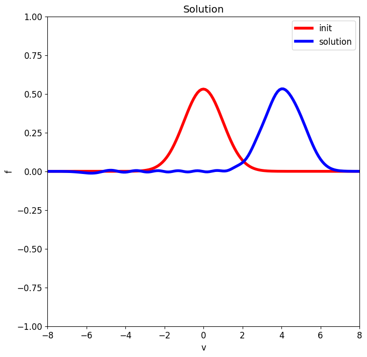
Figure 2: Results of the advection test computed the scheme (12) at time $t_{1}=1$ to $t_{4}=4$ ($N=19$ and $\Delta t=0.1$).

In Figures 2-3 we plot the results where the matrix $\overline{D}^{N}$ is obtained with the method of Section 5.1. A numerical recurrence phenomenon [14] with a change of sign is visible if $N$ is odd.

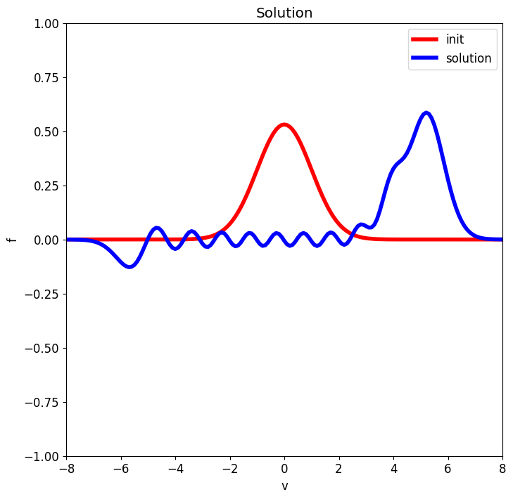
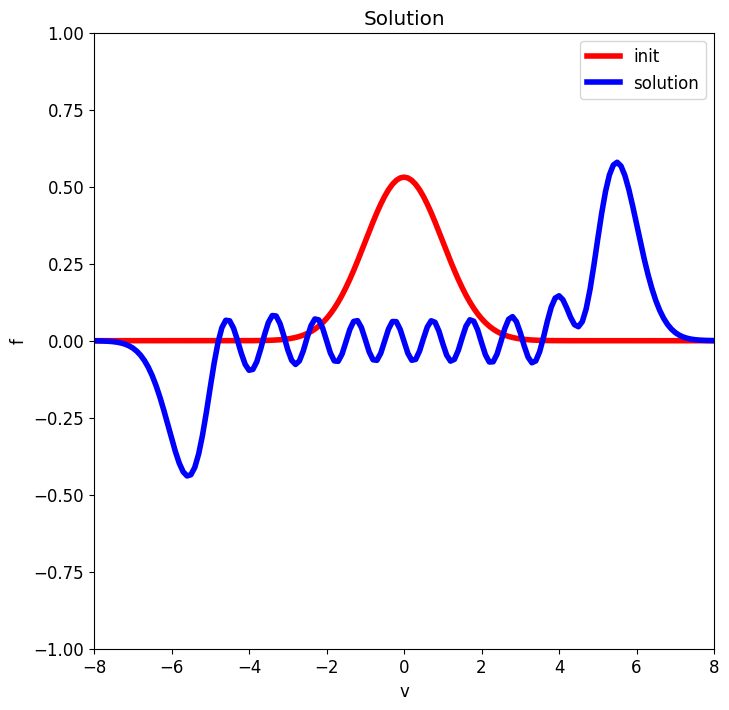
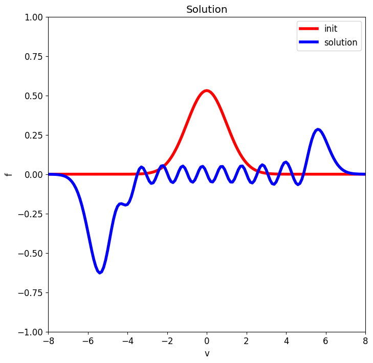
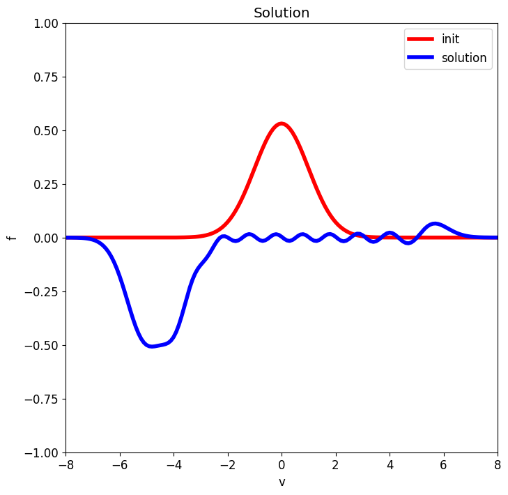
Figure 3: Results of the advection test computed the scheme (12) at time $t_{5}=5$ to $t_{8}=8$ ($N=19$ and $\Delta t=0.1$). No numerical instability even at further time.

In Figure 4 we plot the results where the matrix $\overline{D}^{N}$ is obtained with the method of Section 5.2. The norm $\left<U^{N},A^{N}U^{N}\right>+\varepsilon\|U^{N}\|^{2}$ is rigorously constant one time step after the other, as stated in Lemme 5.10.

Next, we desire to perform a numerical test with the capability to establish the numerical accuracy of the method, even if it is not directly part of the objective of this work. In this case, the parameters $N=19$, $\Delta t=0.1$ and $T=2$. To this aim we propose to start from the known formula [16] which is valid in the sense of distribution

$$\delta(v)=\sum_{m\geq 0}\varphi_{m}(0)\varphi_{m}(v).$$

One has as well in the sense of distribution

$$\delta(v)=\delta(v)e^{-v^{2}/2T}=\sum_{m\geq 0}\varphi_{m}(0)\psi_{m}(v).$$

We consider the initial data

$$U^{N}=(\varphi_{i}(0))_{0\leq i\leq N}.$$

The reference solution is a Dirac mass which moves at velocity $e=1$. In the Figure 5, we plot the initial discrete solution and the numerical solution at time $t=2$ (for convenience all results are post-multiplied by a factor $c=-1$). It is clear at inspection of the Figure 5 that the velocity at which the Dirac evolves is numerically close to $e=1$.

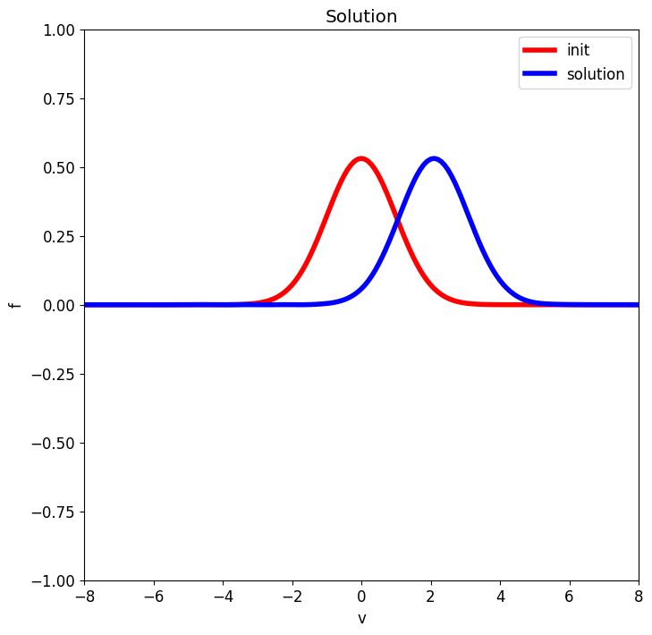
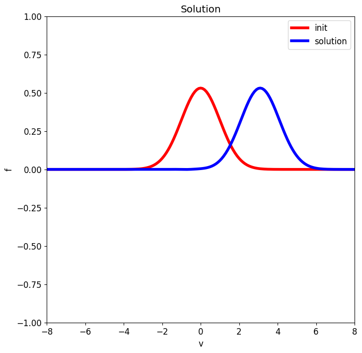
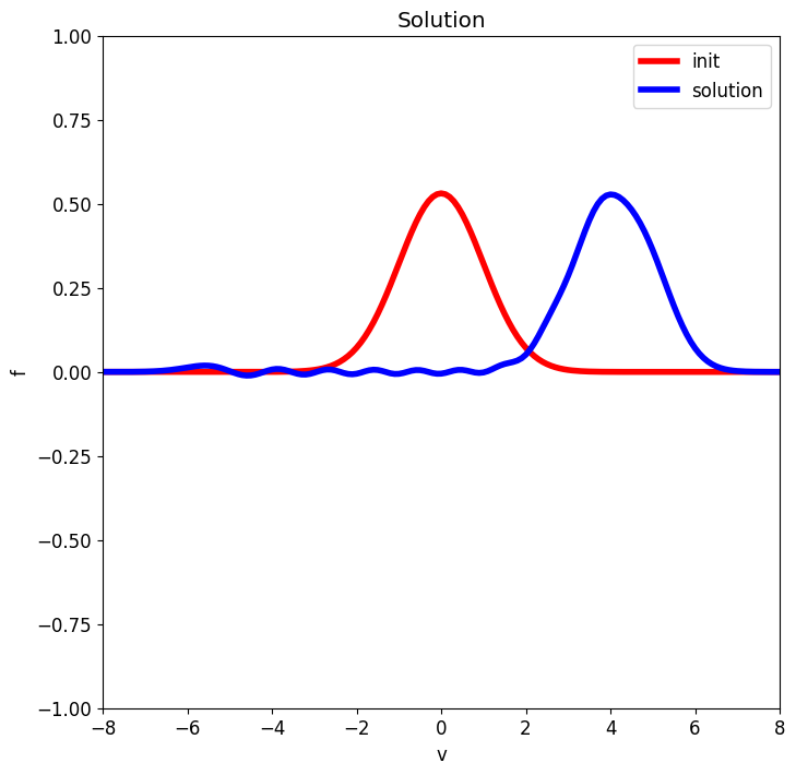
Figure 4: Results of the advection test computed the scheme (12) at time $t_{1}=1$, $t_{2}=2$, $t_{3}=3$ then $t_{4}=4$ ($N=19$ and $\Delta t=0.1$. No numerical instability even at further time.

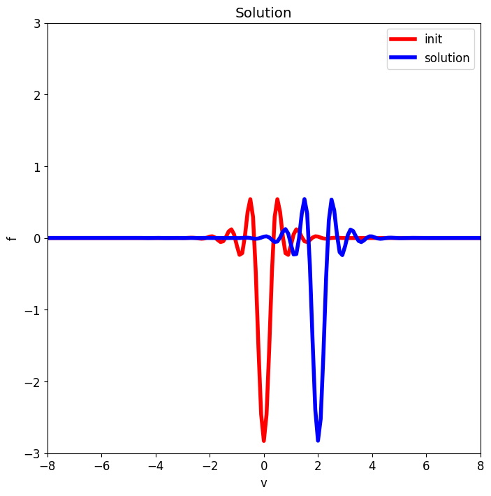
Figure 5: Results of the advection of a Dirac mass (multiplied by -1 for convenience). The final time is $t=2$.

7.2 Diocotron instability

As outlined in Section 6, our method can be employed for solving the Vlasov equation (35) coupled with the Poisson equation. The diocotron instability, observable in magnetized low-density nonneutral plasmas with velocity shear, generates electron vortices akin to the Kelvin-Helmholtz fluidic shear instability. It arises when charge neutrality is disrupted, observed in scenarios like non-neutral electron beams and layers. The magnetic field’s strength induces electron motion dominated by advection within the self-consistent $\mathbf{E}\times\mathbf{B}$ velocity field. The initial non-monotonic electron density profile creates an unstable $\mathbf{E}\times\mathbf{B}$ shear flow, resembling Kelvin-Helmholtz shear layer instability in fluid dynamics and the diocotron instability in beam and plasma physics. As this instability progresses nonlinearly, the initially axisymmetric electron density distribution distorts, resulting in discrete vortices and eventual breakup. This test case holds significance in both fundamental physics and practical applications, such as beam collimation.

The initial condition and the parameters are the same as those in [21], with a uniform external magnetic field $\mathbf{B}=(0,0,5)$ applied along the $z$-axis within a domain of length $L=22$. Additionally, the external electric field is set to $0$ for this particular problem. The initial condition is given by

$$f(t=0,r,v)=\dfrac{C}{2\pi}\exp\left\{\frac{-|\mathbf{v}|^{2}}{2}\right\}\exp\left\{\frac{-(r-L/4)^{2}}{2(0.03L)^{2}}\right\},$$

where $r=\sqrt{(x-L/2)^{2}+(y-L/2)^{2}}$, and the constant $C$ is selected to ensure that the overall electron charge $Q_{e}$ equals $-400$. The time integrator employs a time step of $\Delta t=0.01$, and the simulation is executed until the final time $T=10.0$.

We consider three distinct methods. The first method is the original one without stabilization. The second method is with the first stabilization method. The third method implements the simplification explained in Remark 5.9, that is we nullify the first coefficients of the modified matrices.

We perform tests at $N=40$. For finite difference grid, we test a grid resolution of $64$. We are interested in the way our new methods recover the quadratic stability.

(a) time$=0$

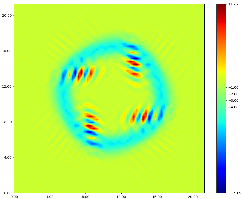
(b) time$=3.80$

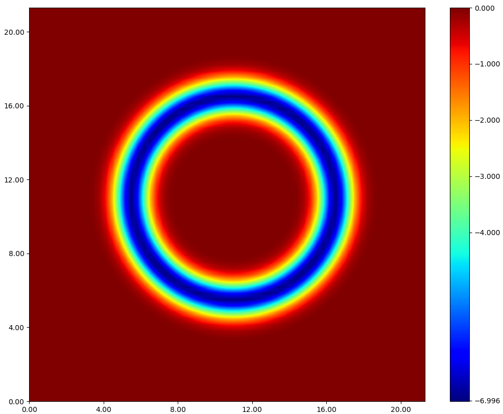
(c) time$=0$

(d) time$=3.80$

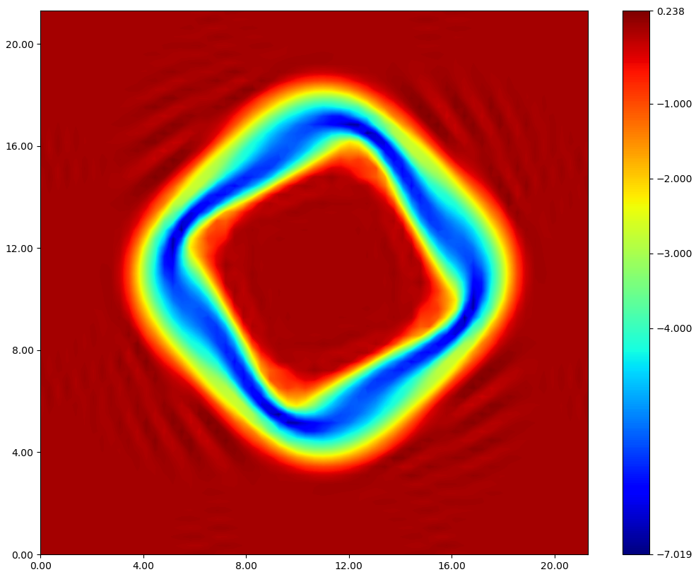
(e) time$=10$

(f) time$=0$

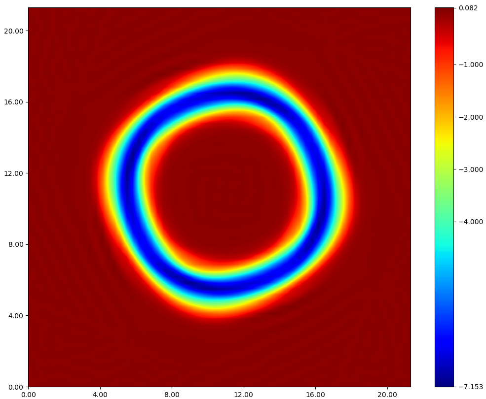
(g) time$=3.80$

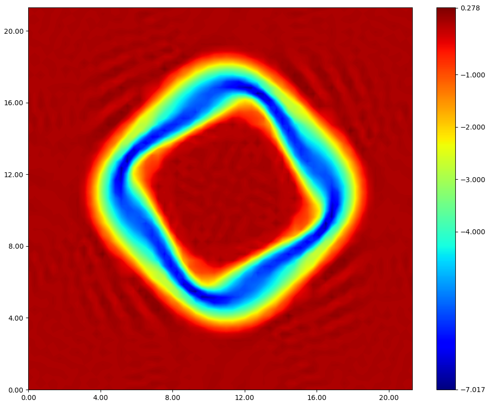
(h) time$=10$

Figure 6: 2D diocotron instability: Evolution of electron charge density over time utilizing three distinct methods: the unstabilized method (first row), the stabilized method (second row), and the numerically conservative method (third row). These visualisations are based on a $64^{2}$ mesh grid. Each figure’s color bar displays the respective minimum and maximum values of the charge densities.

Fig. 6 illustrates how the electron charge density changes over time, for the unstabilized method (first row), the stabilized method (second row) and the stabilized method conservative in mass (third row). From the first row one can observe the numerical instability ($t=3.80$), and the blow-up. From the second and third rows, one can observe that two methods are well stabilized for all times. The results in the third row closely align with the results presented in the second row, based on visual standards. Conversely, none of the three methods enforces the positivity of the particle distribution function, resulting in minor oscillations around zero values.

7.3 Two-stream instability

We take the data of the two stream instability from [5]. The initial data is

$$f_{0}(x,v)=\frac{2}{7}\left(1+\cos kx+\alpha(\cos 2kx+\cos 3kx)/1.2\right)(1+v^{2})\frac{1}{\sqrt{2\pi}}e^{-v^{2}/2}$$

with $\alpha=0.01$ and $k=0.5$. For this problem only two moments are non zero, which are $u_{0}(x)=\frac{12}{7}\left(1+\cos kx+\alpha(\cos 2kx+\cos 3kx)/1.2\right)$ and $u_{2}(x)=\frac{10\sqrt{2}}{7}\left(1+\cos kx+\alpha(\cos 2kx+\cos 3kx)/1.2\right)$. All other moments vanish. The results are shown in Figure 7 and 8. The density function calculated at time $t=20$ is represented together with the history of the norm of the electric field with respect to the time variable. Up to a multiplicative constant, the norm of the electric field is in accordance with the result from [5].

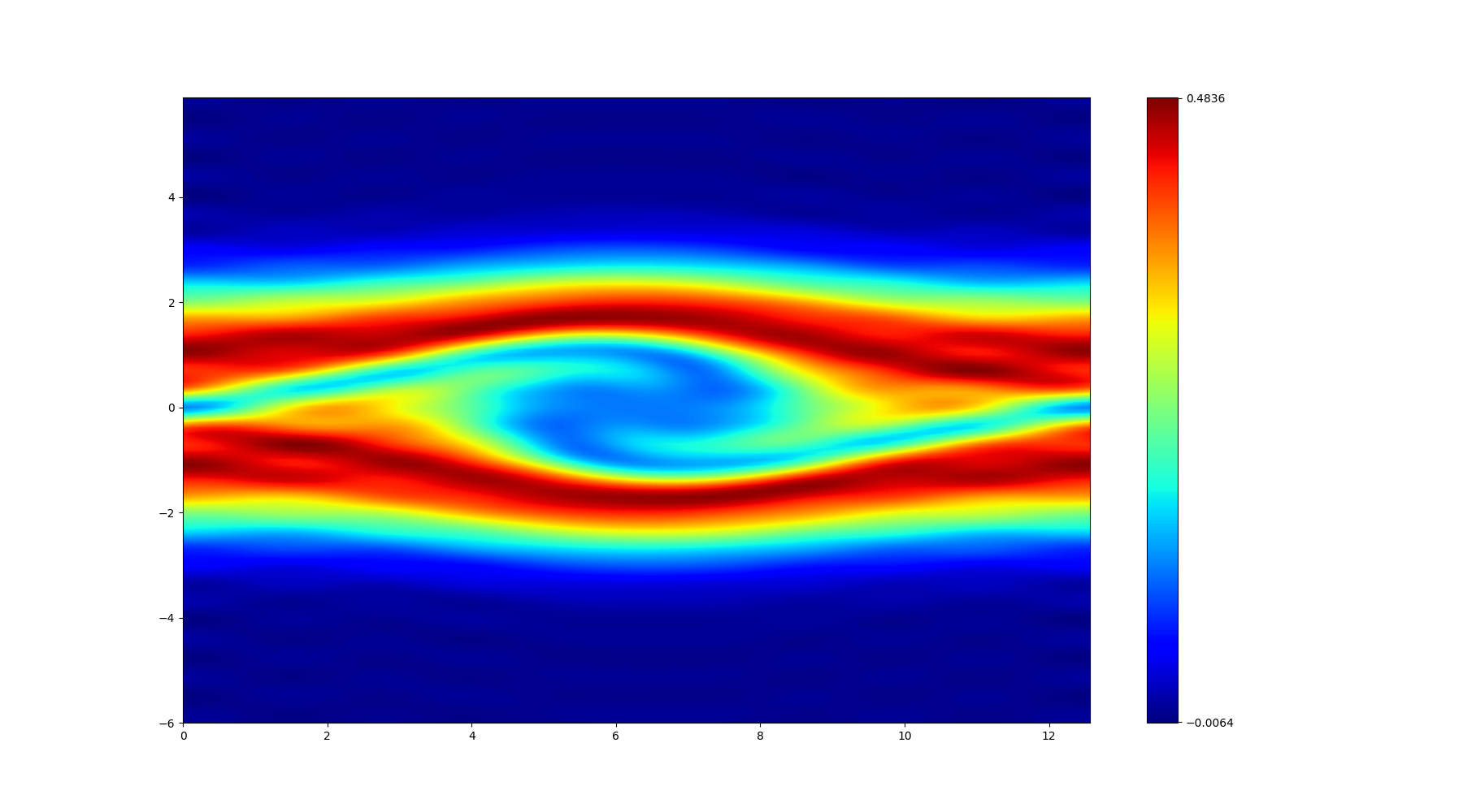
Figure 7: Density function at time $t=20$.

In our opinion our numerical results illustrate that the stabilization of the asymmetric Hermite functions has a potential for the computation of such non linear dynamics without any post-processing or filtering of the numerical results.

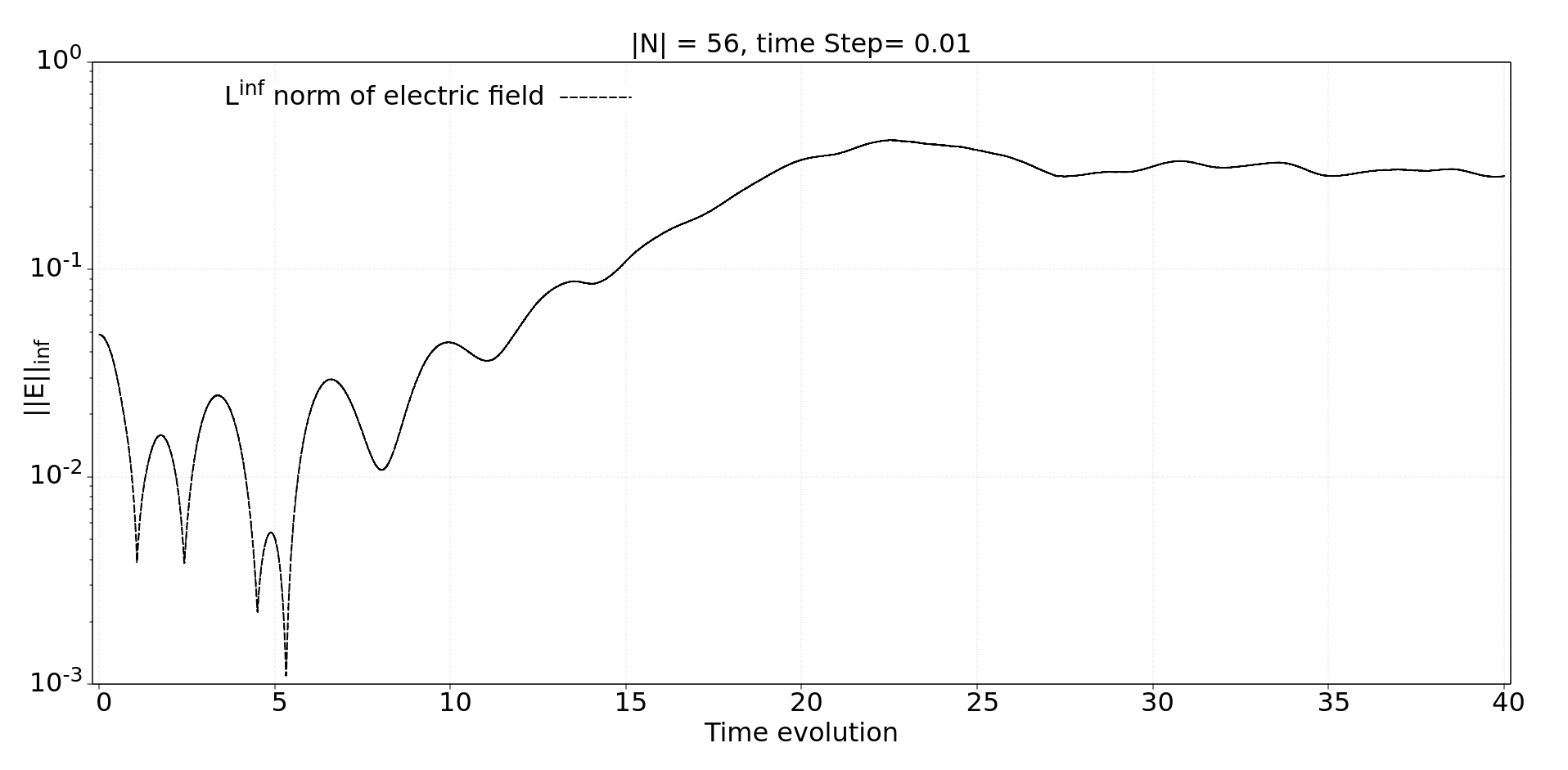
Figure 8: History of the electric field norm with respect to the time variable.

Acknowledments. Both authors deeply thank Sever Hirstoaga and Frédérique Charles whose remarks were essential during the elaboration stage of this work.

Funding. This study has been supported by ANR MUFFIN ANR-19-CE46-0004.

References

• [1] T. P. Armstrong, R. C. Harding, G. Knorr, and D. Montgomery. Solution of Vlasov’s equation by transform methods. Methods in Computational Physics, 9:29-86, 1970.
• [2] M. Bessemoulin-Chatard and F. Filbet, On the stability of conservative discontinuous Galerkin/Hermite spectral methods for the Vlasov-Poisson system, Journal of Computational Physics, Volume 451, 2022.
• [3] S. Le Bourdiec, F. De Vuyst, and L. Jacquet. Numerical solution of the Vlasov-Poisson system using generalized Hermite functions. Computer physics communications, 175(8):528-544, 2006.
• [4] F. Charles, B. DesprΓ©s, R. Dai and S. A. Hirstoaga, Discrete moments models for Vlasov equations with non constant strong magnetic limit, Comptes Rendus. MΓ©canique, Volume 351, S1, 307-329, 2023.
• [5] F. Filbet and T. Xiong. Conservative Discontinuous Galerkin/Hermite Spectral Method for the Vlasov-Poisson System. Communications on Applied Mathematics and Computation, 4(1): 34-59, 2022.
• [6] D. Funaro, G. Manzini. Stability and conservation properties of Hermite-based approximations of the Vlasov-Poisson system. Journal of Scientific Computing, 88(1), 29, 2021.
• [7] H. Gajewski and K. Zacharias. On the convergence of the Fourier-Hermite transformation method for the Vlasov equation with an artificial collision term. Journal of Mathematical Analysis and Applications, 61(3):752-773, 1977.
• [8] J. P. Holloway. Spectral velocity discretizations for the Vlasov-Maxwell equations. Transport Theory Stat. Phys., 25(1):1-32, 1996.
• [9] A. J. Klimas. A numerical method based on the Fourier-Fourier transform approach for modeling 1-D electron plasma evolution. Journal of Computational Physics, 50(2):270-306, 1983.
• [10] K. Kormann, A. Yurova. A generalized Fourier-Hermite method for the Vlasov-Poisson system. BIT Numerical Mathematics, 61(3), 881-909, 2021.
• [11] O. Koshkarov, G. Manzini, G. L. Delzanno, C. Pagliantini, and V. Roytershtein. The multi-dimensional Hermite-discontinuous Galerkin method for the Vlasov-Maxwell equations. Technical Report LA-UR-19-29578, Los Alamos National Laboratory, 2019.
• [12] W. Magnus, F. Oberhettinger and R. P. Soni, Formulas and Theorems for the Special Functions of Mathematical Physics, Grundlehren der mathematischen Wissenschaften (GL, volume 52), 1996.
• [13] G. Manzini, D. Funaro and G. L. Delzanno, Convergence of spectral discretizations of the Vlasov-Poisson system, SIAM J. Numer. Anal, Vol. 55, n. 5 (2017), pp. 2312-2335.
• [14] M. Mehrenberger, L. Navoret and N. Pham, Recurrence phenomenon for Vlasov-Poisson simulations on regular finite element mesh, Commun. in Comput. Phys., 2020.
• [15] C. Pagliantini, G. L. Delzanno, S. Markidis. Physics-based adaptivity of a spectral method for the Vlasov–Poisson equations based on the asymmetrically-weighted Hermite expansion in velocity space. Journal of Computational Physics, 112252, 2023.
• [16] F. W. Olver, D. W. Lozier, R. Boisvert and C. W. Clark, The NIST Handbook of Mathematical Functions, Cambridge University Press, New York, NY, 2010.
• [17] J. T. Parker and P. J. Dellar. Fourier-Hermite spectral representation for the Vlasov-Poisson system in the weakly collisional limit. Journal of Plasma Physics, 81(2):305810203, 2015.
• [18] J. W. Schumer and J. P. Holloway. Vlasov simulations using velocity-scaled Hermite representations. J. Comput. Phys., 144(2):626-661, 1998.
• [19] G. Szego, Orthogonal Polynomials, AMS, 1955.
• [20] Saad, Youcef, and Martin H. Schultz. GMRES: A generalized minimal residual algorithm for solving nonsymmetric linear systems. SIAM Journal on scientific and statistical computing 7.3 (1986): 856-869.
• [21] Sriramkrishnan Muralikrishnan, Antoine J. Cerfon, Matthias Frey, Lee F. Ricketson, Andreas Adelmann, Sparse grid-based adaptive noise reduction strategy for particle-in-cell schemes, Journal of Computational Physics: X, Volume 11, 2021, 100094, ISSN 2590-0552.