Convergence analysis of three semi-discrete numerical schemes for nonlocal geometric flows including perimeter terms

Abstract

We present and analyze three distinct semi-discrete schemes for solving nonlocal geometric flows incorporating perimeter terms. These schemes are based on the finite difference method, the finite element method, and the finite element method with a specific tangential motion. We offer rigorous proofs of quadratic convergence under $H^{1}$-norm for the first scheme and linear convergence under $H^{1}$-norm for the latter two schemes. All error estimates rely on the observation that the error of the nonlocal term can be controlled by the error of the local term. Furthermore, we explore the relationship between the convergence under $L^{\infty}$-norm and manifold distance. Extensive numerical experiments are conducted to verify the convergence analysis, and demonstrate the accuracy of our schemes under various norms for different types of nonlocal flows.

MSCcodes: 65M60, 65M12, 35K55

Keywords: Nonlocal geometric flows; Finite difference method; Finite element method; Tangential motion; Error analysis; Manifold distance

1 Introduction

In this paper, we analyze and establish the convergence result of three distinct numerical methods for evolving a closed plane curve $\Gamma(t)$ under a nonlocal flow that involves perimeter. The normal velocity of $\Gamma(t)$ is determined by the formula

$$\mathcal{V}=\left(\kappa-f(L)\right){\mathcal{N}},$$ (1.1)

where $\kappa$ represents the curvature of the curve, $f$ is a Lipschitz function, $L$ is the perimeter, and ${\mathcal{N}}$ is the unit inner normal vector. Equation (1.1) encompasses a wide range of geometric flows, including:

$$f(L)=\begin{cases}\frac{2\pi}{L},&\text{for area-preserving curve shortening flow of simple curves \cite[cite]{[\@@bibref{}{Gage1986}{}{}]} },\\ \frac{2\pi\,\mathrm{ind}(\Gamma)}{L},&\text{for area-preserving curve shortening flow of nonsimple curves \cite[cite]{[\@@bibref{}{Wang2014}{}{}]}},\\ \frac{2\pi-\beta}{L},&\text{for curve flows with a prescribed rate of change of area \cite[cite]{[\@@bibref{}{Dallaston2016,Tsai2018}{}{}]}},\end{cases}$$

where $\beta\in(-\infty,\infty)$, $\mathrm{ind}(\Gamma)\in{\mathbb{Z}}$ denotes the rational index [19] of a nonsimple curve $\Gamma$. The inclusion of an additional nonlocal force, $f(L)$, enables us to control the area change of an evolving curve. Indeed, by the theorem of turning tangents [19], the rate of area change can be determined by [13]

$$\frac{\mathrm{d}A}{\mathrm{d}t}=\int_{\Gamma}\mathcal{V}\cdot{\mathcal{N}}\mathrm{d}s=\begin{cases}0,\quad&\text{for}\quad f(L)=\frac{2\pi}{L}\quad\text{and simple curves},\\ 0,\quad&\text{for}\quad f(L)=\frac{2\pi\,\mathrm{ind}(\Gamma)}{L}\quad\text{and nonsimple curves},\\ -\beta,\quad&\text{for}\quad f(L)=\frac{2\pi-\beta}{L}\quad\text{and simple curves}.\end{cases}$$

In this paper, we focus on the study of curve evolutions that maintain their topological characteristics.

In recent years, there has been significant emphasis on the development of theoretical and modeling frameworks for nonlocal geometric flows. One prominent instance of such work is the area-preserving curve shortening flow (AP-CSF), which has become vital in the field of image processing [24, 36, 35] and can be interpreted as a limit of the nonlocal model of the Ginzburg-Laudau equation [7]. The existence and convergence results of AP-CSF for both simple and nonsimple closed curve cases have been extensively explored [23, 41]. Moreover, the study of curve flows with a prescribed rate of change in the enclosed area has arisen in connection with the investigation of contracting bubbles in fluid mechanics [9, 10, 11], and the long-time behavior of such flows has been addressed in [39]. For more comprehensive theoretical studies related with nonlocal geometric flows, we refer to [8, 25, 38].

Extensive numerical methods have been employed to simulate the AP-CSF and curve flows with a prescribed rate of change in the enclosed area. Examples of such methods for the AP-CSF include the finite difference method [29], the MBO method [34], the crystalline algorithm [40], as well as PFEMs [32, 6]. Additionally, a rescaled spectral collocation scheme was proposed in [11] for closed embedded plane curves with a prescribed rate of change in the enclosed area. However, there has been relatively little research on the numerical analysis of these methods. Recently, in [26], the authors proposed a semi-discrete finite element method for the AP-CSF of simple curves and established its convergence in $H^{1}$-norm. The nonlocal nature of the geometric equations presents a major challenge for the error analysis.

In this paper, we propose three numerical schemes for nonlocal geometric flows involving perimeter (1.1) and give their error estimates. Our main observation is that the difference between the nonlocal term and its discrete version can be managed through the disparity of the local term. Specifically, we introduce the following three different types of semi-discrete schemes:

• Firstly, we employ a finite difference method to discretize the parametrization equation of (1.1)

  $$\begin{split}&\partial_{t}X=\frac{1}{|\partial_{\xi}X|}\partial_{\xi}\Big{(}\frac{\partial_{\xi}X}{|\partial_{\xi}X|}\Big{)}-f(L)\Big{(}\frac{\partial_{\xi}X}{|\partial_{\xi}X|}\Big{)}^{\perp},\quad\xi\in{\mathbb{S}}^{1},\end{split}$$ (1.2)

  where ${\mathbb{S}}^{1}=[0,2\pi]$, $(a,b)^{\perp}:=(-b,a)$ denotes a clockwise rotation by $\pi/2$ and the periodic function $X(\xi,t):{\mathbb{S}}^{1}\times[0,T]\rightarrow\mathbb{R}^{2}$ is a parameterization of the closed curve $\Gamma\subset\mathbb{R}^{2}$. Under certain appropriate assumptions, we demonstrate that the resulting semi-discrete scheme converges quadratically in the discrete $H^{1}$-norm as defined in [15]. The proof is based on a careful Taylor expansion result and an averaged approximation of the normal vector.

• Secondly, we utilize a finite element method for a natural weak formulation of (1.2). The derived semi-discrete scheme is based on our previous work on AP-CSF of simple curves [26]. An $H^{1}$-optimal error estimate follows from our key observation mentioned above.

• Thirdly, we introduce an artificial tangential motion and apply a finite element method for an alternative parametrization of the geometric equation

  $$\partial_{t}X=\frac{\partial_{\xi\xi}X}{|\partial_{\xi}X|^{2}}-f(L){\mathcal{N}}.$$ (1.3)

  This form of reparametrization was initially proposed by Deckelnick and Dziuk for the curve shortening flow [12] to improve the mesh quality during evolution. It was later interpreted as a DeTurck trick by Elliot and Fritz in [22]. Recently, the DeTurck trick has been further applied to various geometric flows such as elastic flow [33], anisotropic curve shortening flow [17, 16, 14] and fourth-order flows [18]. We emphasize that we have successfully extended the DeTurck trick to the general nonlocal flow case. The resulting semi-discrete scheme yields an asymptotic equidistribution property, as well as an $H^{1}$-optimal error estimate.

As a byporduct, we further explore the convergence of the schemes under manifold distance, a topic extensively discussed in the numerical computation community [4, 5, 42, 27, 28]. We prove that, for simple curves, convergence in the function $L^{\infty}$-norm implies convergence under the manifold distance. Moreover, we prove an optimal convergence of the finite difference scheme under the manifold distance.

The rest of this paper is organized as follows. In Section 2, we briefly introduce the mathematical notations. In Section 3, we propose the semi-discrete schemes and provide the error estimates for the finite difference method. In Section 4, we consider the finite element method, and the finite element method with a tangential motion. Section 5 aims to establishing a connection between the convergence of the manifold distance and $L^{\infty}$-norm. Section 6 presents extensive numerical experiments for the three different numerical schemes and various types of nonlocal flows. The numerical results demonstrate our convergence analysis results in both the $H^{1}$-norm and the manifold distance. Moreover, a better mesh quality is achieved for the finite element method with the aid of tangential motions. Finally, we draw some conclusions in Section 7.

2 Notations

Throughout the paper, we denote the quantities related to the real solution and discrete solution by capital and lower-case letters, respectively. Specifically, for the solution of (1.2), we denote ${\mathcal{T}}=\frac{\partial_{\xi}X}{|\partial_{\xi}X|}$ and ${\mathcal{N}}={\mathcal{T}}^{\perp}$ by the tangent and inner normal of the curve, respectively. Thus (1.2) can be simply written as

$$\partial_{t}X=\frac{1}{|\partial_{\xi}X|}\partial_{\xi}{\mathcal{T}}-f(L){\mathcal{N}},\quad\xi\in{\mathbb{S}}^{1};\qquad X(\xi,0)=X^{0}(\xi).$$ (2.1)

Direct computation gives

$$\partial_{t}|\partial_{\xi}X|=\partial_{t}\partial_{\xi}X\cdot{\mathcal{T}}=\partial_{\xi}(\partial_{t}X\cdot{\mathcal{T}})-\partial_{t}X\cdot\partial_{\xi}{\mathcal{T}}=-|\partial_{\xi}X||\partial_{t}X|^{2}-f(L)|\partial_{\xi}X|\partial_{t}X\cdot\mathcal{N}.$$ (2.2)

For spatial discretization, we utilize a uniform mesh, where the equidistributed grid points ${\mathcal{G}}_{h}:=\{\xi_{1},\ldots,\xi_{N}\}\subset{\mathbb{S}}^{1}$ are given by $\xi_{j}=jh,j=0,\ldots,N$ for $h=2\pi/N$ with $N\geq 2$. We use a periodic index, i.e., $a_{j}=a_{j\pm N}$ when involved. Denote $X_{j}=X(\xi_{j})$, $\dot{X}_{j}=\partial_{t}X(\xi_{j})$, and set

$$Q_{j}=|X_{j}-X_{j-1}|,\quad\mathcal{T}_{j}=\frac{X_{j}-X_{j-1}}{Q_{j}},\quad j=1,\ldots,N.$$

Let $x_{h}:{\mathcal{G}}_{h}\rightarrow{\mathbb{R}}^{2}$ be a grid function. We define the discrete length element $q_{j}$, the discrete tangent $\tau_{j}$ and normal $n_{j}$ as

$$q_{j}=|x_{j}-x_{j-1}|,\quad\tau_{j}=\frac{x_{j}-x_{j-1}}{q_{j}},\quad n_{j}=\tau^{\perp}_{j},$$ (2.3)

where $x_{j}=x_{h}(\xi_{j})$ denotes the vertex of the polygon that approximates the curve. Denote $l_{h}=\sum\limits_{j=1}^{N}q_{j}$ by the perimeter of the polygon. Throughout the article, we denote $C$ by a general constant which is independent of the mesh size $h$ and might vary from line to line.

(Assumption 2.1) Suppose that the solution of (1.2) satisfies $X\in C^{1}\left([0,T],C^{4}({\mathbb{S}}^{1})\right)$, i.e.,

$$K_{1}(X):=\|X\|_{C^{1}\left([0,T],C^{4}({\mathbb{S}}^{1})\right)}<\infty,$$

and there exist constants $0<C_{1}<C_{2}$ such that

$$C_{1}\leq\left|\partial_{\xi}X(\xi,t)\right|\leq C_{2},\quad\forall\ (\xi,t)\in{\mathbb{S}}^{1}\times[0,T].$$ (2.4)

Under this assumption, we have the following results, which have been established in [15].

Lemma 2.1.

[15, Lemmas 3.1, 3.3] Under Assumption 2.1, there exists $h_{0}>0$ such that for $0<h\leq h_{0}$, we have

$$C_{1}\leq Q_{j}/h\leq C_{2},\quad\frac{Q_{j}+Q_{j+1}}{2h}=|\partial_{\xi}X(\xi_{j})|+O(h^{2}),$$ (2.5a)

$${\mathcal{T}}_{j}+{\mathcal{T}}_{j+1}=2\,{\mathcal{T}}(\xi_{j})+O(h^{2}),\quad{\mathcal{T}}_{j}=\frac{1}{2}\left({\mathcal{T}}(\xi_{j})+{\mathcal{T}}(\xi_{j-1})\right)+O(h^{2}),$$ (2.5b)

$$\frac{{\mathcal{T}}_{j+1}-{\mathcal{T}}_{j}}{h}=\partial_{\xi}{\mathcal{T}}(\xi_{j})+O(h^{2}),\quad\frac{\dot{X}_{j+1}-\dot{X}_{j}}{h}=\frac{1}{2}\left(\partial_{t}\partial_{\xi}X(\xi_{j})+\partial_{t}\partial_{\xi}X(\xi_{j+1})\right)+O(h^{2}),$$ (2.5c)

$$\left|\tau_{j+1/2}^{\perp}-{\mathcal{N}}(\xi_{j})\right|\leq\frac{2}{|{\mathcal{T}}_{j}+{\mathcal{T}}_{j+1}|}\left(|{\mathcal{T}}_{j}-\tau_{j}|+|{\mathcal{T}}_{j+1}-\tau_{j+1}|\right)+Ch^{2},$$ (2.5d)

where $\tau_{j+1/2}:=\frac{\tau_{j}+\tau_{j+1}}{|\tau_{j}+\tau_{j+1}|}$ represents the averaged vertex tangent.

For a grid function $u:{\mathcal{G}}_{h}\rightarrow{\mathbb{R}}^{2}$, we define the backward difference quotient as

$$\delta u_{j}:=\frac{u_{j}-u_{j-1}}{h},\quad j=1,\ldots,N.$$

Moreover, to measure the error, we introduce the following discrete norms:

$$\|u\|_{L^{2}_{G}}:=\Bigl{(}h\sum_{j=1}^{N}|u_{j}|^{2}\Bigr{)}^{\frac{1}{2}},\quad\|u\|_{H^{1}_{G}}:=\Bigl{(}h\sum_{j=1}^{N}\bigl{(}|u_{j}|^{2}+|\delta u_{j}|^{2}\bigr{)}\Bigr{)}^{\frac{1}{2}}.$$ (2.6)

3 Finite difference method

In this section, we utilize a finite difference method to solve the equation (1.2).

Definition 3.1.

A semi-discrete finite difference approximation of (1.2) is to find a grid function $x_{h}:{\mathcal{G}}_{h}\times[0,T]\rightarrow{\mathbb{R}}^{2}$ such that

$$\dot{x}_{j}=\frac{2}{q_{j}+q_{j+1}}\left(\tau_{j+1}-\tau_{j}\right)-f(l_{h})\tau^{\perp}_{j+1/2}\quad\text{in }\quad(0,T];\qquad x_{j}(0)=X^{0}(\xi_{j}).$$ (3.1)

Theorem 3.2.

Let $X(\xi,t)$ be a solution of (1.2) satisfying Assumption 2.1. Then there exists $h_{0}>0$ such that for all $0<h\leq h_{0}$, there exists a unique finite difference semi-discrete solution $x_{h}(t)$ in the sense of (3.1). Furthermore, we have the following error estimate

$$\sup_{t\in[0,T]}\|X(t)-x_{h}(t)\|_{H^{1}_{G}}\leq Ch^{2},$$ (3.2)

where the constants $h_{0},C$ depend on $C_{1},C_{2},K_{1}(X),T$ and $f$.

First, we compute the evolution equation for the discrete length $q_{j}$.

Lemma 3.3.

Suppose $x_{h}$ is the finite difference semi-discrete solution in the sense of (3.1), then we have

$$\dot{q}_{j}+\tfrac{q_{j-1}+q_{j}}{4}|\dot{x}_{j-1}|^{2}+\tfrac{q_{j}+q_{j+1}}{4}|\dot{x}_{j}|^{2}+\tfrac{q_{j-1}+q_{j}}{4}f(l_{h})\dot{x}_{j-1}\cdot\tau_{j-1/2}^{\perp}+\tfrac{q_{j+1}+q_{j}}{4}f(l_{h})\dot{x}_{j}\cdot\tau_{j+1/2}^{\perp}=0.$$ (3.3)

Proof   We begin by computing $\dot{q}_{j}$ as

$$\dot{q}_{j} =\left(\dot{x}_{j}-\dot{x}_{j-1}\right)\cdot\tau_{j}$$

$$=\tau_{j}\cdot\left(\frac{2}{q_{j}+q_{j+1}}\left(\tau_{j+1}-\tau_{j}\right)-f(l_{h})\tau_{j+1/2}^{\perp}-\frac{2}{q_{j}+q_{j-1}}\left(\tau_{j}-\tau_{j-1}\right)+f(l_{h})\tau_{j-1/2}^{\perp}\right)$$

$$=\frac{2}{q_{j}+q_{j+1}}\left(\tau_{j}\cdot\tau_{j+1}-1\right)-f(l_{h})\tau_{j+1/2}^{\perp}\cdot\tau_{j}-\frac{2}{q_{j}+q_{j-1}}\left(1-\tau_{j}\cdot\tau_{j-1}\right)+f(l_{h})\tau_{j-1/2}^{\perp}\cdot\tau_{j}$$

$$=\frac{2}{q_{j}+q_{j+1}}\left(\tau_{j}\cdot\tau_{j+1}-1\right)-f(l_{h})\tau_{j+1/2}^{\perp}\cdot\tau_{j}+\frac{2}{q_{j}+q_{j-1}}\left(\tau_{j}\cdot\tau_{j-1}-1\right)-f(l_{h})\tau_{j-1/2}^{\perp}\cdot\tau_{j-1}$$

$$=:J_{j}+J_{j-1},$$ (3.4)

where for the last second equality, we have employed the property

$$\tau_{j-1/2}^{\perp}\cdot\tau_{j}=\tau_{j-1}^{\perp}/|\tau_{j}+\tau_{j-1}|\cdot\tau_{j}=-\tau_{j-1}\cdot\tau_{j}^{\perp}/|\tau_{j}+\tau_{j-1}|=-\tau_{j-1}\cdot\tau_{j-1/2}^{\perp}.$$ (3.5)

Multiplying (3.1) by $\frac{q_{j}+q_{j+1}}{4}f(l_{h})\tau_{j+1/2}^{\perp}$, we obtain

$$\frac{q_{j}+q_{j+1}}{4}f(l_{h})\tau_{j+1/2}^{\perp}\cdot\dot{x}_{j}+\frac{q_{j}+q_{j+1}}{4}f(l_{h})^{2}-f(l_{h})\tau_{j+1/2}^{\perp}\cdot\frac{\tau_{j+1}-\tau_{j}}{2}=0,$$

which can be simplified as

$$\frac{q_{j}+q_{j+1}}{4}f(l_{h})\tau_{j+1/2}^{\perp}\cdot\dot{x}_{j}+\frac{q_{j}+q_{j+1}}{4}f(l_{h})^{2}+f(l_{h})\tau_{j+1/2}^{\perp}\cdot\tau_{j}=0,$$ (3.6)

by using (3.5). Combining (3.1) and (3.6), we get

$$J_{j} =\frac{2}{q_{j}+q_{j+1}}\left(-\frac{1}{2}|\tau_{j}-\tau_{j+1}|^{2}\right)-f(l_{h})\tau_{j+1/2}^{\perp}\cdot\tau_{j}$$

$$=-\frac{1}{q_{j}+q_{j+1}}\left|\dot{x}_{j}+f(l_{h})\tau_{j+1/2}^{\perp}\right|^{2}\left(\frac{q_{j}+q_{j+1}}{2}\right)^{2}-f(l_{h})\tau_{j+1/2}^{\perp}\cdot\tau_{j}$$

$$=-\frac{q_{j}+q_{j+1}}{4}\left(|\dot{x}_{j}|^{2}+2f(l_{h})\tau_{j+1/2}^{\perp}\cdot\dot{x}_{j}+f(l_{h})^{2}\right)-f(L_{h})\tau_{j+1/2}^{\perp}\cdot\tau_{j}$$

$$=-\frac{q_{j}+q_{j+1}}{4}|\dot{x}_{j}|^{2}-\frac{q_{j}+q_{j+1}}{2}f(l_{h})\tau_{j+1/2}^{\perp}\cdot\dot{x}_{j}-\frac{q_{j}+q_{j+1}}{4}f(l_{h})^{2}-f(l_{h})\tau_{j+1/2}^{\perp}\cdot\tau_{j}$$

$$=-\frac{q_{j}+q_{j+1}}{4}|\dot{x}_{j}|^{2}-\frac{q_{j}+q_{j+1}}{4}f(l_{h})\tau_{j+1/2}^{\perp}\cdot\dot{x}_{j}.$$

Plugging this into (3.4) yields (3.3), and the proof is completed. $\Box$

Proof  [Proof of Theorem 3.2]  We define

$$\begin{split}T^{*}=\sup\Bigl{\{}t\in[0,T]:x_{h}\,\,\,\mathrm{solves}\,\,\,\eqref{Semidiscrete,FDM}\,\,\,\text{ with }\,\,\,\tfrac{C_{1}}{2}\leq\frac{q_{j}(t)}{h}\leq 2C_{2},\,\,\,\max_{j=1,\ldots,N}|{\mathcal{T}}_{j}(t)-\tau_{j}(t)|\leq h^{\frac{5}{4}}\Bigr{\}}.\end{split}$$ (3.7)

Clearly $T^{*}>0$. Noticing the nonlinear terms in (3.1) are locally Lipschitz with respect to $x_{j}$, we get local existence and uniqueness using standard ODE theory. Furthermore, since $q_{j}(0)=Q_{j}(0)$ and $\tau_{j}(0)={\mathcal{T}}_{j}(0)$, the desired estimate also holds by continuity. By (3.7) and the Lipschitz continuity of $f$, we have $\forall\ t\in[0,T^{*}]$,

$$\begin{split}2\pi C_{1}\leq L\leq 2\pi C_{2},&\quad\pi C_{1}\leq l_{h}\leq 4\pi C_{2},\quad|f(L)|\leq C,\end{split}$$ (3.8)

where $C$ is a constant depending on $C_{1},C_{2}$ and $f$. We claim that there exists a constant $h_{1}>0$ such that for $0<h\leq h_{1}$, it holds

$$\max_{j=1,\ldots,N}|\dot{x}_{j}(t)|\leq C,\quad\forall\ t\in[0,T^{*}],$$ (3.9)

where $C$ depends on $C_{1},C_{2}$ and $f$. Indeed, by (3.1), (2.5c), (3.7) and (3.8), we obtain

$$|\dot{x}_{j}|^{2} \leq 2\left|\frac{2}{q_{j}+q_{j+1}}\left(\tau_{j+1}-\tau_{j}\right)\right|^{2}+2\left|f(l_{h})\tau_{j+1/2}^{\perp}\right|^{2}\leq C\left|\frac{\tau_{j+1}-\tau_{j}}{h}\right|^{2}+C$$

$$\leq C\left(\left|\frac{{\mathcal{T}}_{j+1}-{\mathcal{T}}_{j}}{h}\right|+\frac{2}{h}\max_{k=1,\ldots,N}|{\mathcal{T}}_{k}-\tau_{k}|\right)^{2}+C\leq C.$$

Moreover, based on (2.5b), we have

$$\min_{j=1,\ldots,N}|{\mathcal{T}}_{j}+{\mathcal{T}}_{j+1}|\geq 1,$$ (3.10)

when $h$ is sufficiently small. Define the truncation error as

$$\mathcal{R}_{j} :=\dot{X}_{j}-\frac{2}{Q_{j}+Q_{j+1}}\left(\mathcal{T}_{j+1}-\mathcal{T}_{j}\right)+f(L){\mathcal{N}}(\xi_{j}),$$ (3.11)

$$\widetilde{\mathcal{R}}_{j} :=\dot{Q}_{j}+\tfrac{Q_{j-1}+Q_{j}}{4}|\dot{X}_{j-1}|^{2}+\tfrac{Q_{j}+Q_{j+1}}{4}|\dot{X}_{j}|^{2}$$

$$\quad+\tfrac{Q_{j-1}+Q_{j}}{4}f(L)\dot{X}_{j-1}\cdot{\mathcal{N}}(\xi_{j-1})+\tfrac{Q_{j+1}+Q_{j}}{4}f(L)\dot{X}_{j}\cdot{\mathcal{N}}(\xi_{j}).$$ (3.12)

1. Estimates of the truncation error $\mathcal{R}_{j},\widetilde{\mathcal{R}}_{j}$. Employing (1.2), (2.5a) and (2.5c), one gets

   $$\begin{split}\mathcal{R}_{j}&=\dot{X}_{j}-\frac{2}{Q_{j}+Q_{j+1}}\left({\mathcal{T}}_{j+1}-{\mathcal{T}}_{j}\right)+f(L){\mathcal{N}}(\xi_{j})\\ &=\dot{X}_{j}-\frac{1}{|\partial_{\xi}X(\xi_{j})|+O(h^{2})}\left(\partial_{\xi}{\mathcal{T}}(\xi_{j})+O(h^{2})\right)+f(L){\mathcal{N}}(\xi_{j})\\ &=\dot{X}_{j}-\frac{1}{|\partial_{\xi}X(\xi_{j})|}\left(1+O(h^{2})\right)\cdot\left(\partial_{\xi}{\mathcal{T}}(\xi_{j})+O(h^{2})\right)+f(L){\mathcal{N}}(\xi_{j})\\ &=\dot{X}_{j}-\frac{1}{|\partial_{\xi}X(\xi_{j})|}\partial_{\xi}{\mathcal{T}}(\xi_{j})+f(L){\mathcal{N}}(\xi_{j})+O(h^{2})\\ &=O(h^{2}).\end{split}$$ (3.13)

   Similarly, applying (2.2), (2.5b) and (2.5c), we derive

   $$\dot{Q}_{j} =\left(\dot{X}_{j}-\dot{X}_{j-1}\right)\cdot{\mathcal{T}}_{j}$$

   $$=\frac{h}{4}\left(\partial_{t}\partial_{\xi}X(\xi_{j-1})+\partial_{t}\partial_{\xi}X(\xi_{j})\right)\cdot\left({\mathcal{T}}(\xi_{j})+{\mathcal{T}}(\xi_{j-1})\right)+O(h^{3})$$

   $$=\frac{h}{2}\partial_{t}\partial_{\xi}X(\xi_{j-1})\cdot{\mathcal{T}}(\xi_{j-1})+\frac{h}{2}\partial_{t}\partial_{\xi}X(\xi_{j})\cdot{\mathcal{T}}(\xi_{j})+O(h^{3})$$

   $$=\frac{h}{2}\left(-|\partial_{\xi}X||\partial_{t}X|^{2}(\xi_{j-1})-f(L)|\partial_{\xi}X|(\xi_{j-1})\partial_{t}X(\xi_{j-1})\cdot{\mathcal{N}}(\xi_{j-1})\right)$$

   $$\quad+\frac{h}{2}\left(-|\partial_{\xi}X||\partial_{t}X|^{2}(\xi_{j})-f(L)|\partial_{\xi}X|(\xi_{j})\partial_{t}X(\xi_{j})\cdot{\mathcal{N}}(\xi_{j})\right)+O(h^{3}),$$

   which together with (2.5a) implies

   $$\begin{split}\widetilde{\mathcal{R}}_{j}&=\dot{Q}_{j}+\frac{Q_{j-1}+Q_{j}}{4}|\dot{X}_{j-1}|^{2}+\frac{Q_{j}+Q_{j+1}}{4}|\dot{X}_{j}|^{2}\\ &\quad+\frac{Q_{j-1}+Q_{j}}{4}f(L)\dot{X}_{j-1}\cdot\mathcal{N}(\xi_{j-1})+\frac{Q_{j+1}+Q_{j}}{4}f(L)\dot{X}_{j}\cdot\mathcal{N}(\xi_{j})=O(h^{3}).\end{split}$$ (3.14)

2. Stability. Denote $e_{j}(t)=X_{j}(t)-x_{j}(t)$. Subtracting (3.1) from (3.11), one gets

   $$\dot{e}_{j}-\frac{2}{q_{j}+q_{j+1}}\left(({\mathcal{T}}_{j+1}-\tau_{j+1})-({\mathcal{T}}_{j}-\tau_{j})\right)$$

   $$= -f(L)\left(\mathcal{N}(\xi_{j})-\tau_{j+1/2}^{\perp}\right)-\left(f(L)-f(l_{h})\right)\tau_{j+1/2}^{\perp}$$

   $$\quad+2\frac{(q_{j}-Q_{j})+(q_{j+1}-Q_{j+1})}{(Q_{j}+Q_{j+1})(q_{j}+q_{j+1})}\left({\mathcal{T}}_{j+1}-{\mathcal{T}}_{j}\right)+\mathcal{R}_{j}$$

   $$= :I^{1}_{j}+I^{2}_{j}+I^{3}_{j}+I^{4}_{j}.$$

   Multiplying both sides with $\frac{1}{2}(q_{j}+q_{j+1})\dot{e}_{j}$ and summing together over all $j=1,\ldots,N$, we obtain

   $$\frac{1}{2}\sum_{j=1}^{N}(q_{j}+q_{j+1})|\dot{e}_{j}|^{2}-\sum_{j=1}^{N}\left(({\mathcal{T}}_{j+1}-\tau_{j+1})-({\mathcal{T}}_{j}-\tau_{j})\right)\cdot\dot{e}_{j}=\sum_{k=1}^{4}\sum_{j=1}^{N}\frac{1}{2}(q_{j}+q_{j+1})I_{j}^{k}\cdot\dot{e}_{j}.$$

   Applying (3.7), Young’s inequality, Assumption 2.1 and (2.5a), we arrive at

   $$-\sum_{j=1}^{N}\left(({\mathcal{T}}_{j+1}-\tau_{j+1})-({\mathcal{T}}_{j}-\tau_{j})\right)\cdot\dot{e}_{j}$$

   $$= \ \frac{1}{2}\frac{\mathrm{d}}{\mathrm{d}t}\sum_{j=1}^{N}q_{j}|{\mathcal{T}}_{j}-\tau_{j}|^{2}+h\sum_{j=1}^{N}\left(\frac{Q_{j}-q_{j}}{Q_{j}}\ \delta\dot{X}_{j}\cdot({\mathcal{T}}_{j}-\tau_{j})+\frac{q_{j}}{2Q_{j}}\left(\delta\dot{X}_{j}\cdot{\mathcal{T}}_{j}\right)|{\mathcal{T}}_{j}-\tau_{j}|^{2}\right)$$

   $$\geq \ \frac{1}{2}\frac{\mathrm{d}}{\mathrm{d}t}\sum_{j=1}^{N}q_{j}|{\mathcal{T}}_{j}-\tau_{j}|^{2}-C\sum_{j=1}^{N}\left(\frac{1}{h}(Q_{j}-q_{j})^{2}+q_{j}|{\mathcal{T}}_{j}-\tau_{j}|^{2}\right),$$

   where for the first equality, we used the result in [15] (cf. page 9 in [15]). Employing (2.5d), (3.7), (3.8), (3.10) and Young’s inequality, we get

   $$\sum_{j=1}^{N}\frac{q_{j}+q_{j+1}}{2}I_{j}^{1}\cdot\dot{e}_{j} \leq\ Ch\sum_{j=1}^{N}\big{|}\mathcal{N}(\xi_{j})-\tau_{j+1/2}^{\perp}\big{|}|\dot{e}_{j}|$$

   $$\leq\ C(\varepsilon)h\sum_{j=1}^{N}|{\mathcal{T}}_{j}-\tau_{j}|^{2}+\varepsilon h\sum_{j=1}^{N}|\dot{e}_{j}|^{2}+C(\varepsilon)h^{4}.$$

   Similarly, using (2.5a), (2.5c), Young’s inequality and (3.13), one obtains

   $$\sum_{j=1}^{N}\frac{1}{2}(q_{j}+q_{j+1})I_{j}^{3}\cdot\dot{e}_{j} \leq\ C\sum_{j=1}^{N}\bigl{(}|Q_{j}-q_{j}|+|Q_{j+1}-q_{j+1}|\bigr{)}|\dot{e}_{j}|$$

   $$\leq\varepsilon h\sum_{j=1}^{N}|\dot{e}_{j}|^{2}+\frac{C(\varepsilon)}{h}\sum_{j=1}^{N}|Q_{j}-q_{j}|^{2},$$

   $$\sum_{j=1}^{N}\frac{1}{2}(q_{j}+q_{j+1})I_{j}^{4}\cdot\dot{e}_{j} \leq\ \varepsilon h\sum_{j=1}^{N}|\dot{e}_{j}|^{2}+C(\varepsilon)h^{4}.$$

   It remains to estimate the term related to $I_{j}^{2}$. Firstly we estimate the error of the perimeter by applying the trapezoidal quadrature formula and (2.5a)

   $$\begin{split}|L-l_{h}|&=\bigg{|}\int_{{\mathbb{S}}^{1}}|\partial_{\xi}X|\ \mathrm{d}\xi-\sum_{j=1}^{N}\frac{q_{j}+q_{j+1}}{2}\bigg{|}\\ &=\bigg{|}h\sum_{j=1}^{N}|\partial_{\xi}X|(\xi_{j})+O(h^{2})-\sum_{j=1}^{N}\frac{q_{j}+q_{j+1}}{2}\bigg{|}\\ &=\bigg{|}\sum_{j=1}^{N}\frac{Q_{j}+Q_{j+1}}{2}+O(h^{2})-\sum_{j=1}^{N}\frac{q_{j}+q_{j+1}}{2}\bigg{|}\\ &\leq\sum_{j=1}^{N}|Q_{j}-q_{j}|+Ch^{2}.\end{split}$$ (3.15)

   This immediately yields

   $$\sum_{j=1}^{N}\frac{1}{2}(q_{j}+q_{j+1})I_{j}^{2}\cdot\dot{e}_{j}\leq \ Ch\sum_{j=1}^{N}|L-l_{h}||\dot{e}_{j}|\leq C(\varepsilon)|L-l_{h}|^{2}+\varepsilon h\sum_{j=1}^{N}|\dot{e}_{j}|^{2}$$

   $$\leq \ C(\varepsilon)\left(\sum_{j=1}^{N}|Q_{j}-q_{j}|\right)^{2}+C(\varepsilon)h^{4}+\varepsilon h\sum_{j=1}^{N}|\dot{e}_{j}|^{2}$$

   $$\leq \ C(\varepsilon)\frac{1}{h}\sum_{j=1}^{N}|Q_{j}-q_{j}|^{2}+C(\varepsilon)h^{4}+\varepsilon h\sum_{j=1}^{N}|\dot{e}_{j}|^{2}.$$

   By combining the above inequalities, (3.7) and choosing $\varepsilon$ to be sufficiently small, we are led to

   $$h\sum_{j=1}^{N}|\dot{e}_{j}|^{2}+\frac{\mathrm{d}}{\mathrm{d}t}\sum_{j=1}^{N}q_{j}|{\mathcal{T}}_{j}-\tau_{j}|^{2}\leq Ch^{4}+C\sum_{j=1}^{N}\left(\frac{1}{h}(Q_{j}-q_{j})^{2}+q_{j}|{\mathcal{T}}_{j}-\tau_{j}|^{2}\right).$$

   Through integration and utilizing Gronwall’s inequality, we obtain

   $$\int^{t}_{0}h\sum_{j=1}^{N}|\dot{e}_{j}|^{2}\ \mathrm{d}s+\sup_{0\leq s\leq t}\sum_{j=1}^{N}q_{j}|{\mathcal{T}}_{j}-\tau_{j}|^{2}\leq Ch^{4}+C\int^{t}_{0}\frac{1}{h}\sum_{j=1}^{N}(Q_{j}-q_{j})^{2}\ \mathrm{d}s,$$ (3.16)

   for $0\leq t\leq T^{*}$, where $C$ is a constant depending on $C_{1},C_{2},K_{1}(X),T$ and $f$.

3. Length difference estimate. By using (3.9) and (3.15), we can derive the following estimates

   $$(|\dot{x}_{j}|^{2}-|\dot{X}_{j}|^{2})\leq(|\dot{x}_{j}|+|\dot{X}_{j}|)|\dot{x}_{j}-\dot{X}_{j}|\leq C|\dot{e}_{j}|,\quad f(l_{h})-f(L)\leq C\sum_{j=1}^{N}|Q_{j}-q_{j}|+Ch^{2}.$$

   Subtracting (3.12) from (3.3), integrating from $0$ to $t$, and applying (2.5d) together with the above estimate, we get

   $$|Q_{j}-q_{j}|(t) \leq\int^{t}_{0}|\dot{Q}_{j}-\dot{q}_{j}|(s)\ \mathrm{d}s+|Q_{j}-q_{j}|(0)$$

   $$\leq C\int^{t}_{0}|q_{j}-Q_{j}|+|q_{j+1}-Q_{j+1}|+|q_{j-1}-Q_{j-1}|\ \mathrm{d}s$$

   $$\quad+Ch\int^{t}_{0}|\tau_{j}-{\mathcal{T}}_{j}|+|\tau_{j+1}-{\mathcal{T}}_{j+1}|+|\tau_{j-1}-{\mathcal{T}}_{j-1}|\ \mathrm{d}s$$

   $$\quad+Ch\int^{t}_{0}\sum_{j=1}^{N}|Q_{j}-q_{j}|\ \mathrm{d}s+Ch^{3}+Ch\int^{t}_{0}|\dot{e}_{j-1}|+|\dot{e}_{j}|\ \mathrm{d}s+\int^{t}_{0}|\widetilde{\mathcal{R}}_{j}|\ \mathrm{d}s.$$

   This together with (3.14) yields

   $$\frac{1}{h}\sum_{j=1}^{N}(Q_{j}-q_{j})^{2}(t) \leq C\int^{t}_{0}h\sum_{j=1}^{N}|\dot{e}_{j}|^{2}\ \mathrm{d}s+C\int^{t}_{0}\frac{1}{h}\sum_{j=1}^{N}(Q_{j}-q_{j})^{2}\ \mathrm{d}s$$

   $$\qquad\qquad+C\int^{t}_{0}h\sum_{j=1}^{N}|{\mathcal{T}}_{j}-\tau_{j}|^{2}\ \mathrm{d}s+Ch^{4}.$$

   Applying Gronwall’s inequality, we get

   $$\begin{split}\frac{1}{h}\sum_{j=1}^{N}(Q_{j}-q_{j})^{2}(t)&\leq C\int^{t}_{0}h\sum_{j=1}^{N}|\dot{e}_{j}|^{2}\ \mathrm{d}s+C\int^{t}_{0}\sum_{j=1}^{N}q_{j}|{\mathcal{T}}_{j}-\tau_{j}|^{2}\ \mathrm{d}s+Ch^{4}\\ &\leq C\int^{t}_{0}h\sum_{j=1}^{N}|\dot{e}_{j}|^{2}\ \mathrm{d}s+C\sup_{0\leq s\leq t}\sum_{j=1}^{N}q_{j}|{\mathcal{T}}_{j}-\tau_{j}|^{2}+Ch^{4}\\ &\leq Ch^{4}+C\int_{0}^{t}\frac{1}{h}\sum_{j=1}^{N}(Q_{j}-q_{j})^{2}(s)ds,\end{split}$$ (3.17)

   where for the last inequality we utilized (3.16). Hence Gronwall’s inequality gives

   $$\frac{1}{h}\sum_{j=1}^{N}(Q_{j}-q_{j})^{2}(t)\leq Ch^{4},\quad 0\leq t\leq T^{*}.$$ (3.18)

   This together with (3.16) implies

   $$\int^{T^{*}}_{0}h\sum_{j=1}^{N}|\dot{e}_{j}|^{2}\ \mathrm{d}s+\sup_{0\leq t\leq T^{*}}\sum_{j=1}^{N}q_{j}|{\mathcal{T}}_{j}-\tau_{j}|^{2}\leq Ch^{4}.$$ (3.19)

Now we are ready to complete the proof by a continuity argument. It follows from (3.19) that there exists $h_{2}>0$ such that when $h\leq h_{2}$,

$$|{\mathcal{T}}_{j}-\tau_{j}|(t)\leq h^{-\frac{1}{2}}\Bigl{(}h\sum_{k=1}^{N}|{\mathcal{T}}_{k}-\tau_{k}|^{2}(t)\Bigr{)}^{\frac{1}{2}}\leq Ch^{-\frac{1}{2}}h^{2}\leq\tfrac{1}{2}h^{\frac{5}{4}},\quad 0\leq t\leq T^{*}.$$

On the other hand, it can be easily derived from (3.18) that

$$|Q_{j}(t)-q_{j}(t)|\leq Ch^{3/2},\quad 0\leq t\leq T^{*},$$

which together with (2.5a) yields

$$\tfrac{2}{3}C_{1}\leq q_{j}(t)/h\leq\tfrac{3}{2}C_{2},\quad h\leq h_{3}.$$

By continuity we can extend $T^{*}$ such that

$$\tfrac{C_{1}}{2}\leq\frac{q_{j}(t)}{h}\leq 2C_{2},\quad\max_{j=1,\ldots,N}|{\mathcal{T}}_{j}(t)-\tau_{j}(t)|\leq h^{\frac{5}{4}}.$$

This contradicts (3.7) if $T^{*}<T$. Therefore, $T^{*}=T$. As for the estimate of $e_{j}$, we first notice

$$\delta e_{j}=\delta X_{j}-\delta x_{j}=\frac{Q_{j}({\mathcal{T}}_{j}-\tau_{j})}{h}+\frac{(Q_{j}-q_{j})}{h}\tau_{j}.$$

Recalling (3.18) and (3.19), we immediately get

$$h\sum_{j=1}^{N}|e_{j}|^{2} \leq C\int^{t}_{0}h\sum_{j=1}^{N}|\dot{e}_{j}|^{2}\mathrm{d}s\leq Ch^{4},$$

$$h\sum_{j=1}^{N}|\delta e_{j}|^{2} \leq Ch\sum_{j=1}^{N}\left(|{\mathcal{T}}_{j}-\tau_{j}|^{2}+\frac{(Q_{j}-q_{j})^{2}}{h^{2}}\right)\leq Ch^{4},$$

which yields

$$\|X(t)-x_{h}(t)\|_{H^{1}_{G}}=\Bigl{(}h\sum_{j=1}^{N}\bigl{(}|e_{j}|^{2}+|\delta e_{j}|^{2}\bigr{)}\Bigr{)}^{\frac{1}{2}}\leq Ch^{2},\quad 0\leq t\leq T,$$

and the proof is completed by taking $h_{0}=\min\{h_{1},h_{2},h_{3}\}$. $\Box$

4 Finite element methods

In this section, we present two finite element methods based on different formulations and establish their error estimates. The parametrization (1.2) naturally leads to a weak formulation: for any $v\in(H^{1}({\mathbb{S}}^{1}))^{2}$, it holds

$$\begin{split}&\int_{{\mathbb{S}}^{1}}|\partial_{\xi}X|\partial_{t}X\cdot v\ \mathrm{d}\xi+\int_{{\mathbb{S}}^{1}}{\mathcal{T}}\cdot\partial_{\xi}v\ \mathrm{d}\xi+\int_{{\mathbb{S}}^{1}}f(L)(\partial_{\xi}X)^{\perp}\cdot v\ \mathrm{d}\xi=0.\end{split}$$ (4.1)

For spatial discretization, let $0=\xi_{0}<\xi_{1}<\ldots<\xi_{N}=2\pi$ be a partition of ${\mathbb{S}}^{1}$. We denote $h_{j}=\xi_{j}-\xi_{j-1}$ as the length of the interval $I_{j}:=[\xi_{j-1},\xi_{j}]$ and $h=\max\limits_{j}h_{j}$. We assume that the partition and the exact solution are regular in the following senses, respectively:

(Assumption 4.1) There exist constants $c_{p}$ and $c_{P}$ such that

$$\min_{j}h_{j}\geq c_{p}h,\quad|h_{j+1}-h_{j}|\leq c_{P}h^{2},\quad 1\leq j\leq N.$$

(Assumption 4.2) Suppose the solution of (1.2) satisfies $X\in W^{1,\infty}\left([0,T],H^{2}({\mathbb{S}}^{1})\right)$, i.e.,

$$K_{2}(X):=\|X\|_{W^{1,\infty}\left([0,T],H^{2}({\mathbb{S}}^{1})\right)}<\infty,$$

and there exist constants $0<C_{1}<C_{2}$ such that (2.4) holds.

We define the following finite element space consisting of piecewise linear functions satisfying periodic boundary conditions:

$$V_{h}=\left\{v\in C({\mathbb{S}}^{1},{\mathbb{R}}^{2}):v|_{I_{j}}\in P_{1}(I_{j}),\quad 1\leq j\leq N,\quad v(\xi_{0})=v(\xi_{N})\right\},$$

where $P_{1}$ denotes all polynomials with degrees at most $1$. For any continuous function $v\in C({\mathbb{S}}^{1},{\mathbb{R}}^{2})$, the linear interpolation $I_{h}v\in V_{h}$ is uniquely determined through $I_{h}v(\xi_{j})=v(\xi_{j})$ for all $1\leq j\leq N$ and can be explicitly written as $I_{h}v(\xi)=\sum\limits_{j=1}^{N}v(\xi_{j})\varphi_{j}(\xi)$, where $\varphi_{j}$ represents the standard Lagrange basis function satisfying $\varphi_{j}(\xi_{i})=\delta_{ij}$.

4.1 FEM with only the normal motion

In this part, we present a finite element method based on the original parametrization (1.2).

Definition 4.1.

We call a function

$$x_{h}(\xi,t)=\sum_{j=1}^{N}x_{j}(t)\varphi_{j}(\xi):{\mathbb{S}}^{1}\times[0,T]\rightarrow{\mathbb{R}}^{2}$$ (4.2)

is a semi-discrete solution of (1.2) if it satisfies $x_{h}(\xi,0)=I_{h}X^{0}$ and for all $v_{h}\in V_{h}$, it holds

$$\int_{{\mathbb{S}}^{1}}q_{h}\partial_{t}x_{h}\cdot v_{h}\ \mathrm{d}\xi+\int_{{\mathbb{S}}^{1}}\tau_{h}\cdot\partial_{\xi}v_{h}\ \mathrm{d}\xi+\int_{{\mathbb{S}}^{1}}\frac{\mathbf{h}^{2}q_{h}}{6}\partial_{\xi}\partial_{t}x_{h}\cdot\partial_{\xi}v_{h}\mathrm{~{}d}\xi+\int_{{\mathbb{S}}^{1}}f(l_{h})(\partial_{\xi}x_{h})^{\perp}\cdot v_{h}\ \mathrm{d}\xi=0,$$ (4.3)

where

$$q_{h}=|\partial_{\xi}x_{h}|=\sum\limits_{j=1}^{N}\frac{q_{j}}{h_{j}}\chi_{I_{j}},\quad\tau_{h}=\frac{\partial_{\xi}x_{h}}{|\partial_{\xi}x_{h}|}=\sum\limits_{j=1}^{N}\frac{x_{j}-x_{j-1}}{q_{j}}\chi_{I_{j}},$$ (4.4)

represent the discrete length element and unit tangent vector, respectively, $l_{h}$ represents the perimeter of the evolved polygon with vertices $x_{j}$, and $\mathbf{h}=\sum\limits_{j=1}^{N}h_{j}\chi_{I_{j}}$ with $\chi$ being the characteristic function.

Remark 4.2.

Compared to the original formulation (4.1), here an extra term $\int_{{\mathbb{S}}^{1}}\frac{\mathbf{h}^{2}|\partial_{\xi}x_{h}|}{6}\partial_{\xi}\partial_{t}x_{h}\cdot\partial_{\xi}v_{h}\mathrm{~{}d}\xi$ is introduced in (4.3), which reduces to the so-called mass-lumped scheme (4.5). Clearly this term does not affect the convergence order for a linear finite element method. As was interpreted in [26, 21], this mass-lumped version can preserve the length shortening property for the CSF/AP-CSF, which was missing for the original formula.

Taking $v_{h}=(\varphi_{j},0)$ and $v_{h}=(0,\varphi_{j})$ for $j=1,\ldots,N$ in (4.3), we are led to the following $2N$ ordinary differential equations:

$$\frac{q_{j}+q_{j+1}}{2}\dot{x}_{j}=\tau_{j+1}-\tau_{j}-f(l_{h})(x_{j+1}-x_{j-1})^{\perp},$$ (4.5)

where $\tau_{j}$ is the discrete tangent defined as (2.3). Furthermore, we have the following identities

$$\dot{q}_{j} =-\frac{1}{q_{j}+q_{j+1}}|\tau_{j+1}-\tau_{j}|^{2}-\frac{1}{q_{j}+q_{j-1}}|\tau_{j-1}-\tau_{j}|^{2}+\tau_{j}\cdot\left(r_{j}-r_{j-1}\right)$$ (4.6)

$$=-\frac{q_{j}+q_{j+1}}{4}|\dot{x}_{j}-r_{j}|^{2}-\frac{q_{j}+q_{j-1}}{4}|\dot{x}_{j-1}-r_{j-1}|^{2}+\tau_{j}\cdot\left(r_{j}-r_{j-1}\right),$$ (4.7)

where for simplicity we denote

$$r_{j}=-f(l_{h})\frac{n_{j}q_{j}+n_{j+1}q_{j+1}}{q_{j}+q_{j+1}}.$$ (4.8)

Theorem 4.3.

Let $X(\xi,t)$ be a solution of (1.2) satisfying Assumption 4.2. Assume that the partition of ${\mathbb{S}}^{1}$ satisfies Assumption 4.1. Then there exists $h_{0}>0$ such that for all $0<h\leq h_{0}$, there exists a unique semi-discrete solution $x_{h}$ for (4.3). Furthermore, the solution satisfies

$$\begin{split}\int^{T}_{0}\|\partial_{t}X-\partial_{t}x_{h}\|^{2}_{L^{2}}\mathrm{d}t+\sup_{t\in[0,T]}\|X-x_{h}\|^{2}_{H^{1}}\leq Ch^{2},\end{split}$$ (4.9)

where $h_{0}$ and $C$ depend on $c_{p},c_{P},C_{1},C_{2},T$, $K_{2}(X)$ and $f$.

Before presenting the proof of Theorem 4.3, we first list a lemma which will be used later.

Lemma 4.4.

[26, Lemma 4.2] Under Assumptions 3.1 and 3.2, suppose further

$$\int_{{\mathbb{S}}^{1}}\left|{\mathcal{T}}-\tau_{h}\right|^{2}q_{h}\mathrm{d}\xi+\||\partial_{\xi}X|-q_{h}\|_{L^{2}}^{2}\leq Ch^{2},\quad\forall\ t\in[0,T^{*}],$$

then there exists a constant $h_{0}$ such that for any $0<h\leq h_{0}$, we have

$$\inf_{\xi}q_{h}\geq 3C_{1}/4,\quad\text{and}\quad\sup_{\xi}q_{h}\leq 3C_{2}/2,\quad\forall\ t\in[0,T^{*}],$$

where $C_{1}$ and $C_{2}$ are the lower and upper bounds of $|\partial_{\xi}X|$ shown in (2.4).

Proof  Similar to the proof of Theorem 3.2, we apply the continuity argument. Define

$$T^{*}=\sup\{t\in[0,T]:\eqref{Semidiscrete1,weak}\,\,\,\text{has a unique solution}\,\,\,x_{h}\,\,\,\text{and}\,\,\,\inf q_{h}\geq C_{1}/2,\,\,\sup q_{h}\leq 2C_{2}\}.$$ (4.10)

Since the nonlinear terms in (4.5) are locally Lipschitz with respect to $x_{j}$, the local existence and uniqueness follow from standard ODE theory, and thus $T^{*}>0$. Moreover, due to the Lipschitz property of $f$ and Assumption (4.10), for any $t\in[0,T^{*}]$, it holds that

$$\begin{split}2\pi C_{1}\leq L\leq 2\pi C_{2},&\quad\pi C_{1}\leq l_{h}\leq 4\pi C_{2},\quad|f(L)|\leq C,\end{split}$$ (4.11)

where $C$ is a constant depending on $C_{1},C_{2},f$.

1. Stability. Taking the difference between (4.1) and (4.3), and choosing $v_{h}=I_{h}(\partial_{t}X)-\partial_{t}x_{h}\in V_{h}$, we get

   $$\quad\int_{{\mathbb{S}}^{1}}|\partial_{t}X-\partial_{t}x_{h}|^{2}q_{h}\mathrm{d}\xi+\int_{{\mathbb{S}}^{1}}\left({\mathcal{T}}-\tau_{h}\right)\left(\partial_{\xi}\partial_{t}X-\partial_{\xi}\partial_{t}x_{h}\right)\mathrm{d}\xi$$

   $$=\int_{{\mathbb{S}}^{1}}\partial_{t}X\cdot(q_{h}-|\partial_{\xi}X|)\left(I_{h}\partial_{t}X-\partial_{t}x_{h}\right)\mathrm{d}\xi+\int_{{\mathbb{S}}^{1}}\frac{\mathbf{h}^{2}q_{h}}{6}\partial_{\xi}\partial_{t}x_{h}\cdot\partial_{\xi}\left(I_{h}\partial_{t}X-\partial_{t}x_{h}\right)\mathrm{d}\xi$$

   $$\quad+\int_{{\mathbb{S}}^{1}}q_{h}(\partial_{t}X-\partial_{t}x_{h})\cdot(\partial_{t}X-I_{h}\partial_{t}X)d\xi+\int_{{\mathbb{S}}^{1}}\left({\mathcal{T}}-\tau_{h}\right)\cdot\left(\partial_{\xi}\partial_{t}X-\partial_{\xi}I_{h}\partial_{t}X\right)\mathrm{d}\xi$$

   $$\quad+\int_{{\mathbb{S}}^{1}}f(L)\left(\partial_{\xi}X-\partial_{\xi}x_{h}\right)^{\perp}\cdot\left(\partial_{t}x_{h}-I_{h}\partial_{t}X\right)\mathrm{d}\xi$$

   $$\quad+\int_{{\mathbb{S}}^{1}}\Big{(}f(L)-f(l_{h})\Big{)}\left(\partial_{\xi}x_{h}\right)^{\perp}\cdot\left(\partial_{t}x_{h}-I_{h}\partial_{t}X\right)\mathrm{d}\xi=:\ J_{1}+J_{2}+J_{3}+J_{4}+J_{5}+J_{6}.$$

   The estimates of the second term on the left side and $J_{j}$ for $1\leq j\leq 4$ can be found in [21, Lemma 5.1] or [26, Lemma 4.1], which can be summarized as follows:

   $$\quad\int_{{\mathbb{S}}^{1}}\left({\mathcal{T}}-\tau_{h}\right)\cdot\left(\partial_{\xi}\partial_{t}X-\partial_{\xi}\partial_{t}x_{h}\right)\mathrm{d}\xi$$

   $$\geq\frac{1}{2}\frac{\mathrm{d}}{\mathrm{d}t}\Big{(}\int_{{\mathbb{S}}^{1}}|\mathcal{T}-\tau_{h}|^{2}q_{h}\mathrm{d}\xi\Big{)}-C\|\partial_{\xi}\partial_{t}X\|_{L^{\infty}}\Big{(}\int_{{\mathbb{S}}^{1}}|{\mathcal{T}}-\tau_{h}|^{2}q_{h}d\xi+\||\partial_{\xi}X|-q_{h}\|_{L^{2}}^{2}\Big{)},$$

   $$J_{1}+J_{2}+J_{3}+J_{4}\leq\varepsilon\int_{\mathbb{S}^{1}}\left|\partial_{t}X-\partial_{t}X_{h}\right|^{2}q_{h}\mathrm{d}\xi+C(\varepsilon)\left\|\partial_{t}X\right\|_{L^{\infty}}^{2}\||\partial_{\xi}X|-q_{h}\|_{L^{2}}^{2}$$

   $$\qquad\qquad\qquad\qquad\qquad\qquad+C(\varepsilon)h^{2}\|\partial_{t}X\|_{H^{1}}^{2}+C\int_{\mathbb{S}^{1}}|\mathcal{T}-\tau_{h}|^{2}q_{h}\mathrm{d}\xi,$$

   where $\varepsilon$ is a generic positive constant which will be chosen later. For $J_{5}$ and $J_{6}$, in view of the Lipschitz property of $f$, (4.11), and the identity

   $$|\partial_{\xi}X-\partial_{\xi}x_{h}|^{2}=(|\partial_{\xi}X|-q_{h})^{2}+|\partial_{\xi}X|q_{h}|\mathcal{T}-\tau_{h}|^{2},$$ (4.12)

   applying similar techniques in [26] (cf. proof of Lemma 4.1), we can get

   $$J_{5} =\int_{{\mathbb{S}}^{1}}f(L)\left(\partial_{\xi}X-\partial_{\xi}x_{h}\right)^{\perp}\cdot\left(\partial_{t}X-I_{h}\partial_{t}X\right)\mathrm{d}\xi$$

   $$\qquad\qquad\qquad+\int_{{\mathbb{S}}^{1}}f(L)\left(\partial_{\xi}X-\partial_{\xi}x_{h}\right)^{\perp}\cdot\left(\partial_{t}x_{h}-\partial_{t}X\right)\mathrm{d}\xi$$

   $$\leq C\left\|\partial_{\xi}X\right\|_{L^{\infty}}\int_{{\mathbb{S}}^{1}}\left|{\mathcal{T}}-\tau_{h}\right|^{2}q_{h}\mathrm{d}\xi+C\int_{{\mathbb{S}}^{1}}(|\partial_{\xi}X|-q_{h})^{2}\mathrm{d}\xi+Ch^{2}\|\partial_{t}X\|_{H^{1}}^{2}$$

   $$\ +C(\varepsilon)\left\|\partial_{\xi}X\right\|_{L^{\infty}}\int_{{\mathbb{S}}^{1}}\left|{\mathcal{T}}-\tau_{h}\right|^{2}q_{h}\mathrm{d}\xi+C(\varepsilon)\||\partial_{\xi}X|-q_{h}\|_{L^{2}}^{2}+\varepsilon\int_{{\mathbb{S}}^{1}}\left|\partial_{t}x_{h}-\partial_{t}X\right|^{2}q_{h}\mathrm{d}\xi,$$

   $$J_{6} =\int_{{\mathbb{S}}^{1}}\big{(}f(L)-f(l_{h})\big{)}\left(\partial_{\xi}x_{h}\right)^{\perp}\cdot\left(\partial_{t}X-I_{h}\partial_{t}X\right)\mathrm{d}\xi$$

   $$\qquad\qquad\qquad+\int_{{\mathbb{S}}^{1}}\big{(}f(L)-f(l_{h})\big{)}\left(\partial_{\xi}x_{h}\right)^{\perp}\cdot\left(\partial_{t}x_{h}-\partial_{t}X\right)\mathrm{d}\xi$$

   $$\leq C|L-l_{h}|^{2}+C\|\partial_{t}X-I_{h}\partial_{t}X\|_{L^{2}}^{2}+C(\varepsilon)|L-l_{h}|^{2}+\varepsilon\int_{{\mathbb{S}}^{1}}q_{h}\left|\partial_{t}x_{h}-\partial_{t}X\right|^{2}\ \mathrm{d}\xi$$

   $$\leq C(\varepsilon)\||\partial_{\xi}X|-q_{h}\|^{2}_{L^{2}}+Ch^{2}\|\partial_{t}X\|^{2}_{H^{1}}+\varepsilon\int_{{\mathbb{S}}^{1}}q_{h}\left|\partial_{t}x_{h}-\partial_{t}X\right|^{2}\ \mathrm{d}\xi.$$

   Here we use the inequalities $|L-l_{h}|^{2}\leq\||\partial_{\xi}X|-q_{h}\|_{L^{1}}^{2}\leq C\||\partial_{\xi}X|-q_{h}\|_{L^{2}}^{2}$. Combining all the above estimates, we are led to

   $$\int_{{\mathbb{S}}^{1}}|\partial_{t}X-\partial_{t}x_{h}|^{2}q_{h}\mathrm{d}\xi+\frac{1}{2}\frac{\mathrm{d}}{\mathrm{d}t}\int_{{\mathbb{S}}^{1}}|\mathcal{T}-\tau_{h}|^{2}q_{h}\mathrm{d}\xi\leq 4\varepsilon\int_{{\mathbb{S}}^{1}}|\partial_{t}X-\partial_{t}x_{h}|^{2}q_{h}\mathrm{d}\xi$$

   $$\qquad+C(\varepsilon)h^{2}\|\partial_{t}X\|^{2}_{H^{2}}+C(\varepsilon,K_{2}(X))\||\partial_{\xi}X|-q_{h}\|_{L^{2}}^{2}+C(\varepsilon,K_{2}(X))\int_{{\mathbb{S}}^{1}}|\mathcal{T}-\tau_{h}|^{2}q_{h}\mathrm{d}\xi.$$

   Choosing $\varepsilon$ small enough, integrating both sides with respect to time from $0$ to $t$ and applying Gronwall’s argument, we arrive at

   $$\int_{0}^{t}\int_{{\mathbb{S}}^{1}}|\partial_{t}X-\partial_{t}x_{h}|^{2}q_{h}\mathrm{d}\xi\mathrm{d}s+\sup\limits_{0\leq s\leq t}\int_{{\mathbb{S}}^{1}}|{\mathcal{T}}-\tau_{h}|^{2}q_{h}\mathrm{d}\xi\leq C\int_{0}^{t}\||\partial_{\xi}X|-q_{h}\|_{L^{2}}^{2}\mathrm{d}s+Ch^{2},$$ (4.13)

   where $C$ is a constant depending on $c_{p}$, $c_{P}$, $C_{1}$, $C_{2}$, $T$, $K_{2}(X)$ and $f$.

2. Length difference estimate. Applying the Lipschitz property of $f$ and (4.11), a mild modification of the proof of [26, Lemma 4.3, Lemma 4.4] enables us to establish the same length difference estimate as in [26]:

   $$\||\partial_{\xi}X|-q_{h}\|_{L^{2}}^{2}\leq C\int_{0}^{t}\int_{{\mathbb{S}}^{1}}\left|\partial_{t}X-\partial_{t}x_{h}\right|^{2}q_{h}\mathrm{d}\xi\mathrm{d}s+C\int^{t}_{0}\int_{{\mathbb{S}}^{1}}\left|{\mathcal{T}}-\tau_{h}\right|^{2}q_{h}\mathrm{d}\xi\mathrm{d}s+Ch^{2},$$ (4.14)

   where $C$ depends on $c_{p}$, $c_{P}$, $C_{1}$, $C_{2}$, $T$, $K_{2}(X)$ and $f$. For the details, we refer to [26].

Combining (4.13) and (4.14), employing Gronwall’s inequality, we derive

$$\int_{0}^{t}\int_{{\mathbb{S}}^{1}}\left|\partial_{t}X-\partial_{t}x_{h}\right|^{2}q_{h}\mathrm{d}\xi\mathrm{d}s+\sup_{0\leq s\leq t}\int_{{\mathbb{S}}^{1}}\left|{\mathcal{T}}-\tau_{h}\right|^{2}q_{h}\mathrm{d}\xi\leq Ch^{2},\quad\forall\ t\in[0,T^{*}],$$ (4.15)

which together with (4.14) yields

$$\||\partial_{\xi}X|-q_{h}\|_{L^{2}}^{2}\leq Ch^{2}.$$

Applying Lemma 4.4, there exists $h_{0}>0$ depending on $c_{p},c_{P},C_{1},C_{2},T$, $K_{2}(X)$ such that for any $0<h\leq h_{0}$, we have

$$\inf q_{h}\geq 3C_{1}/4,\quad\text{and}\quad\sup q_{h}\leq 3C_{2}/2,\quad t\in[0,T^{*}].$$

By standard ODE theory, we can uniquely extend the above semi-discrete solution in a neighborhood of $T^{*}$, and thus $T^{*}=T$. The estimate (4.9) can be concluded similarly as in [26, Theorem 2.5] by integration, (4.12) and (4.15):

$$\quad\|X(\cdot,t)-x_{h}(\cdot,t)\|_{H^{1}}^{2}=\int_{{\mathbb{S}}^{1}}|X-x_{h}|^{2}\mathrm{d}\xi+\int_{{\mathbb{S}}^{1}}|\partial_{\xi}X-\partial_{\xi}x_{h}|^{2}\mathrm{d}\xi$$

$$\leq 2\int_{{\mathbb{S}}^{1}}\big{(}\int_{0}^{t}\partial_{t}X-\partial_{t}x_{h}\mathrm{d}s\big{)}^{2}\mathrm{d}\xi+2\|X^{0}-I_{h}X^{0}\|_{L^{2}}^{2}+\||\partial_{\xi}X|-q_{h}\|_{L^{2}}^{2}+\int_{{\mathbb{S}}^{1}}|\mathcal{T}-\tau_{h}|^{2}|\partial_{\xi}X|q_{h}\mathrm{d}\xi$$

$$\leq 2\int_{{\mathbb{S}}^{1}}T\int_{0}^{t}|\partial_{t}X-\partial_{t}x_{h}|^{2}\mathrm{d}s\mathrm{d}\xi+Ch^{2}\leq Ch^{2},$$

and the proof is completed. $\Box$

4.2 FEM with tangential motions

The aforementioned methods are developed based on the equation (1.1) and only normal motion is allowed. They might suffer from the fact that the mesh will have inhomogeneous properties during the evolution, for instance, some nodes may cluster and the mesh may become distorted. This will lead to instability and even the breakdown of the simulation. To address this challenge, various techniques have been proposed to improve the mesh quality for evolving various types of geometric flows in the literature, such as mesh redistribution [3], and the introduction of artificial tangential velocity [6, 20, 30, 37].

In this subsection, to achieve equipartition property for long-time evolution, we derive another formulation of (1.1) by introducing a tangential velocity. We consider the equation

$$\partial_{t}X=(\kappa-f(L)){\mathcal{N}}+\gamma(X){\mathcal{T}},$$

where ${\mathcal{N}},{\mathcal{T}}$ are the unit normal vector and tangent vector respectively, and $\gamma$ is the tangential velocity to be determined. It is important to note that the presence of tangential velocity has no impact on the shape of evolving curves [12, 22], and suitable choices of tangential velocity may help the redistribution of mesh points [31, 30, 37]. As mentioned in the introduction, inspired by the work of [12, 22] for curve shortening flow, we consider an explicit tangential velocity given by

$$\gamma(X)=\frac{\partial_{\xi}X\cdot\partial_{\xi\xi}X}{|\partial_{\xi}X|^{3}}.$$

More generally, for a fixed parameter $0<\alpha\leq 1$, we consider a series of reparametrizations $X_{\alpha}$ which are determined by

$$\alpha\partial_{t}X_{\alpha}+(1-\alpha)(\partial_{t}X_{\alpha}\cdot{\mathcal{N}}){\mathcal{N}}=\frac{\partial_{\xi\xi}X_{\alpha}}{|\partial_{\xi}X_{\alpha}|^{2}}-f(L){\mathcal{N}};\quad X_{\alpha}(\xi,0)=X^{0}(\xi).$$ (4.16)

Below we provide three justifications for (4.16).

• The solution $X_{\alpha}$ of the evolution equation (4.16) has the same shape as the standard parametrization equation (1.2) since they share the same normal velocity

  $$\partial_{t}X_{\alpha}\cdot{\mathcal{N}} =\alpha\partial_{t}X_{\alpha}\cdot{\mathcal{N}}+(1-\alpha)\partial_{t}X_{\alpha}\cdot{\mathcal{N}}$$

  $$=\left(\frac{\partial_{\xi\xi}X_{\alpha}}{|\partial_{\xi}X_{\alpha}|^{2}}-\gamma(X_{\alpha}){\mathcal{T}}-f(L){\mathcal{N}}\right)\cdot{\mathcal{N}}$$

  $$=\left(\frac{1}{|\partial_{\xi}X_{\alpha}|}\partial_{\xi}\left(\frac{\partial_{\xi}X_{\alpha}}{|\partial_{\xi}X_{\alpha}|}\right)-f(L){\mathcal{N}}\right)\cdot{\mathcal{N}}$$

  $$=\kappa-f(L),$$

  where we note that the curvature $\kappa$ and perimeter $L$ are geometric quantities independent of the parametrization.

• The evolution of (4.16) has asymptotic equidistribution property in a continuous level. More precisely, suppose $X_{\alpha}^{e}$ is the equilibrium of (4.16), i.e., $\partial_{t}X_{\alpha}^{e}=0$, then formally we have

  $$\partial_{\xi}|\partial_{\xi}X_{\alpha}^{e}| =\partial_{\xi\xi}X_{\alpha}^{e}\cdot{\mathcal{T}}=\left(\frac{\partial_{\xi\xi}X_{\alpha}^{e}}{|\partial_{\xi}X_{\alpha}^{e}|^{2}}-f(L){\mathcal{N}}\right)\cdot|\partial_{\xi}X_{\alpha}^{e}|^{2}{\mathcal{T}}=0,$$

  which means the equilibrium has constant arc-length. This leads us to expect that the corresponding numerical solution for (4.16) has equidistributed mesh points for long-time evolution.

• As explained in [22, Section 8], we can write the standard parametrization equation (1.2) as

  $$\partial_{t}X=\Delta_{\Gamma[X]}X-f(L){\mathcal{N}},$$

  where $\Gamma[X]$ is the image of $X$ and $\Delta_{\Gamma[X]}$ is the Laplace-Beltrami operator over the curve $\Gamma[X]$. The DeTurck’s trick for operator $\Delta_{\Gamma[X]}$ maintains the normal term $f(L){\mathcal{N}}$ unaffected and leads to (4.16). In this aspect, the nonlocal flows can be viewed as a natural generalization of [22, Section 8].

Next we present a finite element method for (4.16). For fixed $\alpha$, multiplying $|\partial_{\xi}X|^{2}$ for both sides of (4.16) (below we omit the subscript $\alpha$ for simplicity), we obtain the following weak formulation: for any $\ v\in(H^{1}({\mathbb{S}}^{1}))^{2}$, it holds

$$\int_{{\mathbb{S}}^{1}}|\partial_{\xi}X|^{2}(\alpha\partial_{t}X+(1-\alpha)(\partial_{t}X\cdot{\mathcal{N}}){\mathcal{N}})\cdot v\mathrm{d}\xi+\int_{{\mathbb{S}}^{1}}\partial_{\xi}X\cdot\partial_{\xi}v\mathrm{d}\xi+\int_{{\mathbb{S}}^{1}}f(L)|\partial_{\xi}X|^{2}{\mathcal{N}}\cdot v\mathrm{d}\xi=0.$$ (4.17)

We use the same spatial discretization for ${\mathbb{S}}^{1}$ as in the last subsection and assume it satisfies Assumption 4.1. We further assume the exact solution of (4.16) is regular in the following sense.

(Assumption 4.3) Suppose that the solution of (4.16) with an initial value $X^{0}\in H^{2}({\mathbb{S}}^{1})$ satisfies $X\in W^{1,\infty}\left([0,T],H^{2}({\mathbb{S}}^{1})\right)$, i.e.,

$$K_{2}(X):=\|X\|_{W^{1,\infty}\left([0,T],H^{2}({\mathbb{S}}^{1})\right)}<\infty,$$

and there exist constants $0<C_{1}<C_{2}$ such that (2.4) holds.

Definition 4.5.

We call a function $x_{h}(\xi,t)=\sum\limits_{j=1}^{N}x_{j}(t)\varphi_{j}(\xi):{\mathbb{S}}^{1}\times[0,T]\rightarrow{\mathbb{R}}^{2}$ is a semi-discrete solution of (4.16) if it satisfies $x_{h}(\xi,0)=I_{h}X^{0}$ and

$$\int_{{\mathbb{S}}^{1}}|\partial_{\xi}x_{h}|^{2}(\alpha\partial_{t}x_{h}+(1-\alpha)(\partial_{t}x_{h}\cdot n_{h})n_{h})\cdot v_{h}\ \mathrm{d}\xi+\int_{{\mathbb{S}}^{1}}\partial_{\xi}x_{h}\cdot\partial_{\xi}v_{h}\ \mathrm{d}\xi\\ +\int_{{\mathbb{S}}^{1}}f(l_{h})|\partial_{\xi}x_{h}|^{2}n_{h}\cdot v_{h}\ \mathrm{d}\xi=0,$$ (4.18)

for any $v_{h}\in V_{h}$, where $n_{h}=\tau_{h}^{\perp}$ represents the piecewise unit normal vector.

Theorem 4.6.

Let $X(\xi,t)$ be a solution of (4.16) satisfying Assumption 4.3. Assume that the partition of ${\mathbb{S}}^{1}$ satisfies Assumption 4.1. Then there exists $h_{0}>0$ such that for all $0<h\leq h_{0}$, there exists a unique semi-discrete solution $x_{h}$ for (4.18). Furthermore, the solution satisfies

$$\sup_{t\in[0,T]}|X-x_{h}|_{H^{1}}^{2}+\alpha\int^{T}_{0}\|\partial_{t}X-\partial_{t}x_{h}\|_{L^{2}}^{2}\ \mathrm{d}t +(1-\alpha)\int^{T}_{0}\|n_{h}\cdot(\partial_{t}X-\partial_{t}x_{h})\|_{L^{2}}^{2}\ \mathrm{d}t$$

$$\qquad\qquad\qquad\leq{CTh^{2}+Ce^{MT/\alpha}h^{2}},$$

where $h_{0}$, $C$ and $M$ depend on $c_{p}$, $c_{P}$, $C_{1}$, $C_{2}$, $K_{2}(X)$, and $f$.

Proof  Fix $\alpha\in(0,1]$. We consider a Banach space $Z_{h}=C([0,T],V_{h})$ equipped with the norm

$$\|v_{h}\|_{Z_{h}}:=\sup_{t\in[0,T]}\|v_{h}(t)\|_{L^{2}},\quad v_{h}\in Z_{h},$$

and a nonempty closed convex subset $B_{h}$ of $Z_{h}$ defined by

$$B_{h}:=\bigg{\{}v_{h}\in Z_{h}|\sup_{t\in[0,T]}e^{-Mt/\alpha}\|(\partial_{\xi}X-\partial_{\xi}v_{h})(t)\|_{L^{2}}^{2}\leq K^{2}h^{2}\ \text{and}\ v_{h}(\cdot,0)=I_{h}X^{0}(\cdot)\bigg{\}},$$ (4.19)

where $M,K>0$ are constants that will be determined later. For any $u_{h}\in B_{h}$, applying interpolation error, inverse inequality and (4.19), one can easily derive

$$\|(\partial_{\xi}X-\partial_{\xi}u_{h})(t)\|_{L^{\infty}} \leq\|(\partial_{\xi}X-I_{h}\partial_{\xi}X)(t)\|_{L^{\infty}}+\|(I_{h}\partial_{\xi}X-\partial_{\xi}I_{h}u_{h})(t)\|_{L^{\infty}}$$

$$\leq Ch^{1/2}+Ch^{-1/2}\|(I_{h}\partial_{\xi}X-\partial_{\xi}u_{h})(t)\|_{L^{2}}$$

$$\leq Ch^{1/2}+Ch^{-1/2}\left(\|(\partial_{\xi}X-I_{h}\partial_{\xi}X)(t)\|_{L^{2}}+\|(\partial_{\xi}X-\partial_{\xi}u_{h})(t)\|_{L^{2}}\right)$$

$$\leq Ch^{1/2}\left(1+e^{\frac{Mt}{2\alpha}}K\right).$$

It follows from Assumption 4.3 that there exists a constant $h_{0}>0$ depending on $\alpha,M,$ $K,T,K_{2}(X)$ such that for any $0<h\leq h_{0}$, we have

$$\inf_{\xi}|\partial_{\xi}u_{h}|\geq C_{1}/2,\quad\sup_{\xi}|\partial_{\xi}u_{h}|\leq 2C_{2}.$$ (4.20)

Setting $\widehat{q_{h}}=|\partial_{\xi}u_{h}|$ and denoting $\widehat{l_{h}}$ as the perimeter of $u_{h}$, due to the Lipschitz property of $f$, it holds that

$$\begin{split}2\pi C_{1}\leq L\leq 2\pi C_{2},&\quad\pi C_{1}\leq\widehat{l_{h}}\leq 4\pi C_{2},\quad|f(\widehat{l_{h}})|\leq C,\end{split}$$ (4.21)

where $C$ is a constant depending on $C_{1},C_{2}$ and $f$. We define a continuous map $F:B_{h}\rightarrow Z_{h}$ as follows. For any $u_{h}\in B_{h}$, we define $y_{h}$ as the unique solution of the following linear equation:

$$\begin{split}&\int_{{\mathbb{S}}^{1}}\widehat{q_{h}}^{2}(\alpha\partial_{t}y_{h}+(1-\alpha)(\partial_{t}y_{h}\cdot\widehat{n_{h}})\widehat{n_{h}})\cdot v_{h}\ \mathrm{d}\xi+\int_{{\mathbb{S}}^{1}}\partial_{\xi}y_{h}\cdot\partial_{\xi}v_{h}\ \mathrm{d}\xi\\ &\qquad\qquad+\int_{{\mathbb{S}}^{1}}f(\widehat{l_{h}})\widehat{q_{h}}(\partial_{\xi}y_{h})^{\perp}\cdot v_{h}\ \mathrm{d}\xi=0,\quad\forall\ v_{h}\in V_{h},\end{split}$$ (4.22)

with initial data $y_{h}(0)=I_{h}X^{0}$, where $\widehat{n_{h}}=\left(\frac{\partial_{\xi}u_{h}}{|\partial_{\xi}u_{h}|}\right)^{\perp}$.

1. Length difference estimate for $u_{h}\in B_{h}$. Applying (4.19) and the triangle inequality, we obtain

   $$\|(|\partial_{\xi}X|-\widehat{q_{h}})(t)\|_{L^{2}}\leq\|(\partial_{\xi}X-\partial_{\xi}u_{h})(t)\|_{L^{2}}\leq Khe^{Mt/(2\alpha)},\quad 0\leq t\leq T.$$ (4.23)

2. Stability estimate for $y_{h}\in Z_{h}$. Taking $v=v_{h}$ in (4.17) and subtracting (4.22) from (4.17), we get

   $$\int_{{\mathbb{S}}^{1}}\widehat{q_{h}}^{2}\left(\alpha\left(\partial_{t}X-\partial_{t}y_{h}\right)\cdot v_{h}+(1-\alpha)\left(\partial_{t}X-\partial_{t}y_{h}\right)\cdot\widehat{n_{h}}(\widehat{n_{h}}\cdot v_{h})\right)\ \mathrm{d}\xi$$

   $$\qquad\qquad\qquad+\int_{{\mathbb{S}}^{1}}\left(\partial_{\xi}X-\partial_{\xi}y_{h}\right)\cdot\partial_{\xi}v_{h}\ \mathrm{d}\xi$$

   $$= \ \int_{{\mathbb{S}}^{1}}(\widehat{q_{h}}^{2}-|\partial_{\xi}X|^{2})(\alpha\partial_{t}X\cdot v_{h}+(1-\alpha)(\partial_{t}X\cdot\widehat{n_{h}})(\widehat{n_{h}}\cdot v_{h}))\ \mathrm{d}\xi$$

   $$+(1-\alpha)\int_{{\mathbb{S}}^{1}}|\partial_{\xi}X|^{2}(\partial_{t}X\cdot(\widehat{n_{h}}-{\mathcal{N}})(\widehat{n_{h}}\cdot v_{h})+(\partial_{t}X\cdot{\mathcal{N}})(\widehat{n_{h}}-{\mathcal{N}})\cdot v_{h})\ \mathrm{d}\xi$$

   $$+\int_{{\mathbb{S}}^{1}}\left(-f(L)|\partial_{\xi}X|+f(\widehat{l_{h}})\widehat{q_{h}}\right)(\partial_{\xi}X)^{\perp}\cdot v_{h}\ \mathrm{d}\xi$$

   $$-\int_{{\mathbb{S}}^{1}}f(\widehat{l_{h}})\widehat{q_{h}}\left((\partial_{\xi}X)^{\perp}-(\partial_{\xi}y_{h})^{\perp}\right)\cdot v_{h}\ \mathrm{d}\xi=:\ J_{1}+J_{2}+J_{3}+J_{4}.$$

   Choosing $v_{h}=I_{h}(\partial_{t}X)-\partial_{t}y_{h}\in V_{h}$, the estimates of the left-hand hand side and $J_{1},J_{2}$ can be found in [22, (3.7)], which can be summarized as

   $$\begin{split}&\quad\frac{\mathrm{d}}{\mathrm{d}t}\|\partial_{\xi}X-\partial_{\xi}y_{h}\|^{2}_{L^{2}}+\frac{C_{1}^{2}}{8}\alpha\|\partial_{t}X-\partial_{t}y_{h}\|^{2}_{L^{2}}+\frac{C_{1}^{2}}{4}(1-\alpha)\|\widehat{n_{h}}\cdot(\partial_{t}X-\partial_{t}y_{h})\|^{2}_{L^{2}}\\ &\leq\ Ch^{2}(1+\|\partial_{t}X\|^{2}_{H^{2}})+\|\partial_{\xi}X-\partial_{\xi}y_{h}\|^{2}_{L^{2}}+Ch^{2}K^{2}e^{Mt/\alpha}/\alpha+2|J_{3}|+2|J_{4}|.\end{split}$$ (4.24)

   For the terms of $J_{3}$ and $J_{4}$, in view of the Lipschitz property of $f$ and the inequality

   $$|L-\widehat{l_{h}}|\leq C\||\partial_{\xi}X|-\widehat{q_{h}}\|_{L^{2}},$$

   applying (4.20), (4.21), (4.23) and Young’s inequality, we get

   $$|J_{3}| =\bigg{|}\int_{{\mathbb{S}}^{1}}\left(-f(L)+f(\widehat{l_{h}})\right)|\partial_{\xi}X|(\partial_{\xi}X)^{\perp}\cdot v_{h}\ \mathrm{d}\xi-\int_{{\mathbb{S}}^{1}}f(\widehat{l_{h}})\left(|\partial_{\xi}X|-\widehat{q_{h}}\right)(\partial_{\xi}X)^{\perp}\cdot v_{h}\ \mathrm{d}\xi\bigg{|}$$

   $$\leq C\int_{{\mathbb{S}}^{1}}|L-\widehat{l_{h}}|\left(|I_{h}(\partial_{t}X)-\partial_{t}X|+|\partial_{t}X-\partial_{t}y_{h}|\right)\ \mathrm{d}\xi$$

   $$\qquad+C\int_{{\mathbb{S}}^{1}}||\partial_{\xi}X|-\widehat{q_{h}}|\left(|I_{h}(\partial_{t}X)-\partial_{t}X|+|\partial_{t}X-\partial_{t}y_{h}|\right)\ \mathrm{d}\xi$$

   $$\leq Ch|L-\widehat{l_{h}}|\|\partial_{t}X\|_{H^{1}}+C|L-\widehat{l_{h}}|\|\partial_{t}X-\partial_{t}y_{h}\|_{L^{2}}$$

   $$\qquad+Ch\||\partial_{\xi}X|-\widehat{q_{h}}\|_{L^{2}}\|\partial_{t}X\|_{H^{1}}+C\||\partial_{\xi}X|-\widehat{q_{h}}\|_{L^{2}}\|\partial_{t}X-\partial_{t}y_{h}\|_{L^{2}}$$

   $$\leq CKe^{\frac{Mt}{2\alpha}}h\|\partial_{t}X-\partial_{t}y_{h}\|_{L^{2}}+CKe^{\frac{Mt}{2\alpha}}h^{2}\|\partial_{t}X\|_{H^{1}}$$

   $$\leq\frac{C(\varepsilon)e^{Mt/\alpha}K^{2}h^{2}}{4\alpha}+\varepsilon\alpha\|\partial_{t}X-\partial_{t}y_{h}\|_{L^{2}}^{2}+\alpha h^{2}\|\partial_{t}X\|_{H^{1}}^{2},$$

   and

   $$|J_{4}| =\bigg{|}\int_{{\mathbb{S}}^{1}}f(\widehat{l_{h}})\widehat{q_{h}}\left((\partial_{\xi}X)^{\perp}-(\partial_{\xi}y_{h})^{\perp}\right)\cdot v_{h}\ \mathrm{d}\xi\bigg{|}$$

   $$\leq Ch\|\partial_{\xi}X-\partial_{\xi}y_{h}\|_{L^{2}}\|\partial_{t}X\|_{H^{1}}+C\|\partial_{\xi}X-\partial_{\xi}y_{h}\|_{L^{2}}\|\partial_{t}X-\partial_{t}y_{h}\|_{L^{2}}$$

   $$\leq\|\partial_{\xi}X-\partial_{\xi}y_{h}\|_{L^{2}}^{2}+Ch^{2}\|\partial_{t}X\|_{H^{1}}^{2}+\frac{C(\varepsilon)}{4\alpha}\|\partial_{\xi}X-\partial_{\xi}y_{h}\|_{L^{2}}^{2}+\varepsilon\alpha\|\partial_{t}X-\partial_{t}y_{h}\|_{L^{2}}^{2}.$$

   Combining all the above estimate and taking $\varepsilon$ small enough, we obtain

   $$\begin{split}&\quad\frac{\mathrm{d}}{\mathrm{d}t}\|\partial_{\xi}X-\partial_{\xi}y_{h}\|_{L^{2}}^{2}+\frac{C_{1}^{2}}{16}\alpha\|\partial_{t}X-\partial_{t}y_{h}\|_{L^{2}}^{2}+\frac{C_{1}^{2}}{4}(1-\alpha)\|\widehat{n_{h}}\cdot(\partial_{t}X-\partial_{t}y_{h})\|_{L^{2}}^{2}\\ &\leq\ Ch^{2}+C(1+1/\alpha)\|\partial_{\xi}X-\partial_{\xi}y_{h}\|^{2}_{L^{2}}+Ch^{2}K^{2}e^{Mt/\alpha}/\alpha,\end{split}$$ (4.25)

   where $C$ depends on $c_{p}$, $c_{P}$, $C_{1}$, $C_{2}$, $T$, $K_{2}(X)$, and $f$. This directly gives

   $$\frac{\mathrm{d}}{\mathrm{d}t}\|\partial_{\xi}X-\partial_{\xi}y_{h}\|_{L^{2}}^{2}\leq\ Ch^{2}+C(1+1/\alpha)\|\partial_{\xi}X-\partial_{\xi}y_{h}\|^{2}_{L^{2}}+Ch^{2}K^{2}e^{Mt/\alpha}/\alpha.$$

   Thus we get

   $$\|\partial_{\xi}X(t)-\partial_{\xi}y_{h}(t)\|_{L^{2}}^{2}$$

   $$\leq\|\partial_{\xi}X^{0}-\partial_{\xi}y_{h}(0)\|_{L^{2}}^{2}e^{C(1+\frac{1}{\alpha})t}+Ch^{2}\int_{0}^{t}e^{C(1+\frac{1}{\alpha})(t-s)}\left(1+K^{2}e^{Ms/\alpha}/\alpha\right)ds$$

   $$\leq Ce^{C(1+\frac{1}{\alpha})t}h^{2}+CK^{2}h^{2}\frac{e^{\frac{M}{\alpha}t}-e^{C(1+\frac{1}{\alpha})t}}{M-C(1+\alpha)},$$

   which yields

   $$e^{-Mt/\alpha}\|\partial_{\xi}X-\partial_{\xi}y_{h}\|^{2}_{L^{2}}\leq Ch^{2}e^{(-\frac{M}{\alpha}+\frac{C}{\alpha}+C)t}+\frac{CK^{2}h^{2}}{M-C(1+\alpha)}\leq K^{2}h^{2},$$ (4.26)

   if we select $M\geq 3C+C\alpha$ and $K^{2}\geq 2C$. Hence, by plugging (4.26) into (4.25), integrating from $0$ to $T$, we arrive at

   $$\max_{t\in[0,T]} \|\partial_{\xi}X-\partial_{\xi}y_{h}\|^{2}_{L^{2}}+\alpha\int^{T}_{0}\|\partial_{t}X-\partial_{t}y_{h}\|_{L^{2}}^{2}\ \mathrm{d}t+(1-\alpha)\int^{T}_{0}\|\widehat{n_{h}}\cdot(\partial_{t}X-\partial_{t}y_{h})\|_{L^{2}}^{2}\mathrm{d}t$$

   $$\leq C(1+T)h^{2}+CK^{2}h^{2}(1+1/\alpha)\int_{0}^{T}e^{Ms/\alpha}ds$$

   $$\leq C(1+T)h^{2}+K^{2}h^{2}(e^{MT/\alpha}-1)\leq CTh^{2}+Ce^{MT/\alpha}h^{2},$$ (4.27)

   where $C$ and $M$ are constants depending on $c_{p},c_{P},K_{2}(X)$, $C_{1},C_{2}$ and $f$.

Now we complete the proof by applying Schauder’s fixed point theorem for $F$. Indeed, it follows from assumption (4.19) and (4.26) that $F(B_{h})\subset B_{h}$. Furthermore, it can be easily derived from (4.27) and the assumption $y_{h}(0)=I_{h}X^{0}$ that $\|y_{h}\|_{W^{1,2}([0,T],V_{h})}\leq C$, which, together with the Sobolev embedding, implies that the inclusion $F(B_{h})\subset B_{h}$ is compact. Thus, by Schauder’s fixed point theorem (c.f. [22, Theorem 3.1]), there exists a fixed point $x_{h}$ for (4.22) that satisfies $F(x_{h})=x_{h}$, which is the desired semi-discrete solution. Moreover, the estimate (4.27) also holds for the solution $x_{h}$.

To address the uniqueness, it is important to recognize that (4.18) constitutes a nonlinear ODE system for $x_{j}$. Consequently, the uniqueness of $x_{h}$ is assured by nonlinear ODE theory. It’s evident that $x_{h}$ serves as a semi-discrete solution of (4.18) and thus aligns with the corresponding estimate. $\Box$

5 Convergence under manifold distance

As discussed in [42, 27], for two closed simple curves $\Gamma_{1}$ and $\Gamma_{2}$, the manifold distance is defined as:

$$\mathrm{M}\left(\Gamma_{1},\Gamma_{2}\right):=\mathrm{Area}((\Omega_{1}\setminus\Omega_{2})\cup(\Omega_{2}\setminus\Omega_{1}))=\mathrm{Area}(\Omega_{1})+\mathrm{Area}(\Omega_{2})-2\mathrm{Area}(\Omega_{1}\cap\Omega_{2}),$$

where $\Omega_{1}$ and $\Omega_{2}$ are the regions enclosed by $\Gamma_{1}$ and $\Gamma_{2}$ respectively. As proved in [42, Proposition 5.1], the manifold distance satisfies symmetry, positivity and the triangle inequality. Under some assumptions, e.g., If $\Gamma_{2}$ lies within the tabular neighborhood of the $C^{2}$ curve $\Gamma_{1}$ [13], the manifold distance between the two curves can be interpreted as the $L^{1}$-norm of the distance function. Recently, compare to the $L^{p}$-norm of parametrization functions, this type of distance (i.e. the $L^{p}$-norm of distance function) has gained wide attentions in both the scientific computing [27, 28] and numerical analysis community [1]. Moreover, the authors’ works [42, 27, 28] have demonstrated that the manifold distance (one of the shape metrics) is more suitable than the norm of parametrization functions for quantifying numerical errors of the schemes which are used for solving geometric flows, especially for schemes which allow intrinsic tangential velocity. Meanwhile, Bai and Li [1] have recently observed that the $L^{2}$-norm of distance function (so-called the projected distance in their paper) leads to the recovery of full $H^{1}$ parabolicity, and established a convergence result for Dziuk’s scheme of the mean curvature flow with finite elements of degree $k\geq 3$.

In this subsection, we first show that the function $L^{\infty}$-norm is stronger than the manifold distance under some suitable regularity assumptions. More specifically, for a parametrization function $X\in C^{2}({\mathbb{S}}^{1})$ of curve $\Gamma_{X}$ and an approximation curve $\Gamma_{Y}$ by parameterization function $Y\in C^{0}({\mathbb{S}}^{1})$, we have the following lemma.

Lemma 5.1.

Let $X:{\mathbb{S}}^{1}\rightarrow{\mathbb{R}}^{2}$ be a parametrization function of simple curves $\Gamma_{X}$ with $X\in C^{2}({\mathbb{S}}^{1})$, and assume there exist constants $0<C_{1}<C_{2}$ such that (2.4) holds. Then there exist positive constants $\delta_{0}$ and $C$ such that for any parametrization function $Y\in C^{0}({\mathbb{S}}^{1})$ satisfying

$$\|X-Y\|_{L^{\infty}}\leq\delta_{0},$$

the following inequality holds:

$$\mathrm{M}(\Gamma_{X},\Gamma_{Y})\leq C\|X-Y\|_{L^{\infty}},$$

where $\Gamma_{X}$ and $\Gamma_{Y}$ are the images of $X$ and $Y$, respectively. The constants $\delta_{0}$ and $C$ depend on $X$, $C_{1}$ and $C_{2}$.

Proof  The closed simple $C^{2}$ curve $\Gamma_{X}$ in ${\mathbb{R}}^{2}$ naturally admits a tabular neighborhood $\Omega_{\delta}$ in the following manner [2, 13]: there exists a constant $\delta>0$ such that the mapping

$$E_{X}:\Gamma_{X}\times(-\delta,\delta)\rightarrow{\mathbb{R}}^{2},\quad E_{X}(a,\eta)=a+\eta{\mathcal{N}},$$

acts as a diffeomorphism from $\Gamma_{X}\times(-\delta,\delta)$ to the image denoted by $\mathrm{Im}(E_{X})=:\Omega_{\delta}$. Here ${\mathcal{N}}$ represents the normal vector along $\Gamma_{X}$. Consequently, the points within the tabular neighborhood $\Omega_{\delta}$ can be represented as

$$E_{X}^{-1}:\Omega_{\delta}\rightarrow\Gamma_{X}\times(-\delta,\delta),\quad E_{X}^{-1}(b)=(\pi_{\Gamma_{X}}(b),d_{\Gamma_{X}}(b)),$$

where $\pi_{\Gamma_{X}}(b)\in\Gamma_{X}$ is the projection of $b$ onto $\Gamma_{X}$, and $d_{\Gamma_{X}}(b)=d(b,\Gamma_{X})$ represents the signed distance.

Set $\delta_{0}<\delta$. For any parametrization function $Y\in C^{0}({\mathbb{S}}^{1})$ which satisfies $\|X-Y\|_{L^{\infty}}\leq\delta_{0}$, it is evident that $\Gamma_{Y}\subseteq\Omega_{\delta}$. Now define

$$\delta_{w}:=\sup_{b\in\Gamma_{Y}}|d_{\Gamma_{X}}(b)|$$

which represents the maximum distance between $\Gamma_{Y}$ and $\Gamma_{X}$. Clearly, we can assume $\delta_{w}>0$, as there is nothing to prove otherwise. Define two curves $\Gamma_{\delta_{w}}^{\mathrm{int}}$ and $\Gamma_{\delta_{w}}^{\mathrm{{ext}}}$, within the tabular neighborhood $\Omega_{\delta}$, which are parametrized as

$$\begin{split}{\mathbb{S}}^{1}\ni\xi\rightarrow(x_{\mathrm{int}}(\xi),y_{\mathrm{int}}(\xi))=(x(\xi),y(\xi))-\delta_{w}{\mathcal{N}}(x(\xi),y(\xi)),\\ {\mathbb{S}}^{1}\ni\xi\rightarrow(x_{\mathrm{ext}}(\xi),y_{\mathrm{ext}}(\xi))=(x(\xi),y(\xi))+\delta_{w}{\mathcal{N}}(x(\xi),y(\xi)),\end{split}$$ (5.1)

respectively. Here $X(\xi)=(x(\xi),y(\xi))$ is a parametrization of the curve $\Gamma_{X}$, and ${\mathcal{N}}$ is the corresponding unit normal vector. Denote $\Omega_{\delta_{w}}$ as the region enclosed by $\Gamma_{\delta_{w}}^{\mathrm{int}}$ and $\Gamma_{\delta_{w}}^{\mathrm{{ext}}}$ (cf. Fig 1 (a)).

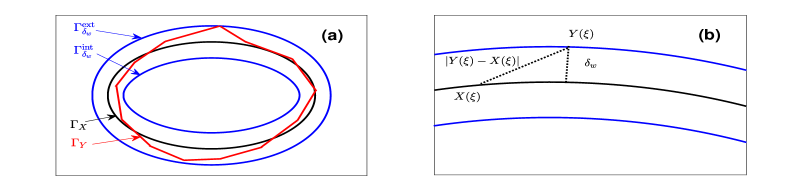
Figure 1: Illustration of (a) the definition of $\Gamma_{X},\Gamma_{Y},\Gamma_{\delta_{w}}^{\mathrm{int}}$ and $\Gamma_{\delta_{w}}^{\mathrm{{ext}}}$, (b) the comparison of the projection distance $\delta_{w}$ and the function $L^{\infty}$-norm $\|X-Y\|_{L^{\infty}}$.

By utilizing the regularity assumption of $X$ along with (2.4) and (5.1), we can estimate the area of $\Omega_{\delta_{w}}$ as follows:

$$\mathrm{Area}(\Omega_{\delta_{w}}) =\int_{{\mathbb{S}}^{1}}\partial_{\xi}x_{\mathrm{ext}}\cdot y_{\mathrm{ext}}\ \mathrm{d}\xi-\int_{{\mathbb{S}}^{1}}\partial_{\xi}x_{\mathrm{int}}\cdot y_{\mathrm{int}}\ \mathrm{d}\xi$$

$$\leq C\int_{{\mathbb{S}}^{1}}|\partial_{\xi}x_{\mathrm{ext}}-\partial_{\xi}x_{\mathrm{int}}|+|y_{\mathrm{ext}}-y_{\mathrm{int}}|\ \mathrm{d}\xi$$

$$\leq C\delta_{w}\int_{{\mathbb{S}}^{1}}|\partial_{\xi}{\mathcal{N}}|+|{\mathcal{N}}|\ \mathrm{d}\xi\leq C\delta_{w},$$

where $C$ is a constant depending on $X,C_{1}$ and $C_{2}$. The triangle inequality for manifold distance yields

$$\mathrm{M}(\Gamma_{X},\Gamma_{Y})\leq\mathrm{M}(\Gamma_{X},\Gamma_{\delta_{w}}^{\mathrm{int}})+\mathrm{M}(\Gamma_{\delta_{w}}^{\mathrm{int}},\Gamma_{Y})\leq 2\mathrm{Area}(\Omega_{\delta_{w}})\leq C\delta_{w}\leq C\|X-Y\|_{L^{\infty}},$$

where we use the natural control $\delta_{w}\leq\|X-Y\|_{L^{\infty}}$ (cf. Fig 1 (b)) and the proof is completed. $\Box$

As natural corollaries, we have following convergence results of numerical schemes under the manifold distance.

Corrolary 5.2.

We have the following convergence results under the manifold distance.

1. Let $X(\xi,t)$ be the solution of (1.2) satisfying Assumption 2.1 and $X\in W^{3,2}({\mathbb{S}}^{1})$. Let $x_{h}(t)$ be the unique finite difference semi-discrete solution of (3.1). Then we have

   $$\sup_{t\in[0,T]}\mathrm{M}(\Gamma_{X},\Gamma_{x_{h}})\leq Ch^{2}.$$

2. Let $X(\xi,t)$ be the solution of (1.2) satisfying Assumption 4.2 and $X\in W^{3,2}({\mathbb{S}}^{1})$. Assume that the partition of ${\mathbb{S}}^{1}$ satisfies Assumption 4.1 and $x_{h}(t)$ is the unique finite element semi-discrete solution of (4.3). Then we have

   $$\sup_{t\in[0,T]}\mathrm{M}(\Gamma_{X},\Gamma_{x_{h}})\leq Ch.$$

3. Let $X(\xi,t)$ be the solution of (4.16) satisfying Assumption 4.3 and $X\in W^{3,2}({\mathbb{S}}^{1})$. Assume that the partition of ${\mathbb{S}}^{1}$ satisfies Assumption 4.1 and $x_{h}(t)$ is the unique finite element semi-discrete solution of (4.18). Then we have

   $$\sup_{t\in[0,T]}\mathrm{M}(\Gamma_{X},\Gamma_{x_{h}})\leq Ch.$$

For all the estimates, $\Gamma_{X}$ and $\Gamma_{x_{h}}$ represent the images of $X$ and $x_{h}$, respectively, and the constant $C$ depends on $C_{1},C_{2},T$, $f$ and additionally, $K_{1}(X)$ for (1) and $K_{2}(X)$ for (2) and (3).

Proof   For the first conclusion, combining the Sobolev embedding, triangle inequality, interpolation error, Lemma 5.3 with the main error estimate (3.2), one obtains

$$\|X-x_{h}\|_{L^{\infty}} \leq C\|X-x_{h}\|_{H^{1}}\leq C\|X-I_{h}X\|_{H^{1}}+C\|I_{h}X-x_{h}\|_{H^{1}}$$

$$\leq Ch^{2}\|X\|_{W^{3,2}}+C\|I_{h}X-x_{h}\|_{H^{1}_{G}}\sqrt{1+h^{2}/6}\leq Ch^{2},$$

where for the third inequality we have utilized Lemma 5.3 for the grid function $I_{h}X-x_{h}$. Hence, by applying Lemma 5.1 with $\delta_{0}=Ch^{2}$, $Y=x_{h}$ and for different time $t\in[0,T]$, we conclude the first assertion (1). The latter two statements can be similarly confirmed by referring to Theorems 4.3 and 4.6, along with the Sobolev embedding

$$\sup_{t\in[0,T]}\|X-x_{h}\|_{L^{\infty}}\leq C\sup_{t\in[0,T]}\|X-x_{h}\|_{H^{1}}\leq Ch,$$

and the proof is completed. $\Box$

Lemma 5.3.

Let $g:{\mathcal{G}}_{h}\rightarrow{\mathbb{R}}$ be a grid function. Then we have

$$\|g\|_{H^{1}}^{2}\leq\|g\|_{H^{1}_{G}}^{2}\left(1+h^{2}/6\right),$$

where we identify a grid function $g$ with the piecewise linear function over ${\mathbb{S}}^{1}$ that connects the grid values of $g$.

Proof   Denote $M_{j}=\max\limits_{\xi\in(\xi_{j},\xi_{j+1})}\left(|g|^{2}\right)^{\prime\prime}$ and by applying the trapezoidal rule, we have

$$\|g\|_{H^{1}}^{2} =\sum_{j=1}^{N}\int_{\xi_{j}}^{\xi_{j+1}}|g|^{2}+|\partial_{\xi}g|^{2}\ \mathrm{d}\xi$$

$$\leq\sum_{j=1}^{N}\left(\frac{|g(\xi_{j})|^{2}+|g(\xi_{j+1})|^{2}}{2}h+\frac{h^{3}}{12}M_{j}\right)+h\sum_{j=1}^{N}|\delta g_{j}|^{2}$$

$$=h\sum_{j=1}^{N}\bigl{(}|g_{j}|^{2}+|\delta g_{j}|^{2}\bigr{)}+\frac{h^{3}}{12}\sum_{j=1}^{N}M_{j}.$$

Noticing $g$ is a piecewise linear function, we have

$$M_{j}=\max\limits_{\xi\in(\xi_{j},\xi_{j+1})}\left(|g|^{2}\right)^{\prime\prime}=2\max_{\xi\in(\xi_{j},\xi_{j+1})}|g^{\prime}|^{2}=2|\delta g_{j+1}|^{2},$$

which yields

$$\|g\|_{H^{1}}^{2}\leq h\sum_{j=1}^{N}\bigl{(}|g_{j}|^{2}+|\delta g_{j}|^{2}\bigr{)}+\frac{h^{3}}{6}\sum_{j=1}^{N}|\delta g_{j+1}|^{2}\leq\|g\|_{H^{1}_{G}}^{2}\left(1+\frac{1}{6}h^{2}\right),$$

and the proof is completed. $\Box$

6 Numerical results

In this section, we present numerous numerical experiments for the proposed three different schemes applied to various geometric flows involving the nonlocal term $f(L)$. We first provide full discretizations for the three schemes using backward Euler time discretization. Specifically, we choose an integer $m$, set the time step $\tau=T/m$ and $t_{k}=k\tau$ for $k=0,\ldots,m$. Given a fixed mesh size $h$ and a time step $\tau=O(h^{2})$, we consider the following three cases.

• For the finite difference method (3.1), given $x_{h}^{0}=I_{h}X^{0}$, for $k\geq 1$, we consider the solution $x_{h}^{k}\in{\mathcal{G}}_{h}$ of the following equation (denoted as FDM)

  $$\frac{x_{j}^{k}-x_{j}^{k-1}}{\tau}=\frac{2}{q^{k-1}_{j}+q_{j+1}^{k-1}}\left(\frac{x^{k}_{j+1}-x^{k}_{j}}{q^{k-1}_{j+1}}-\frac{x^{k}_{j}-x^{k}_{j-1}}{q^{k-1}_{j}}\right)-f(l_{h}^{k-1})\frac{n_{j}^{k-1}+n^{k-1}_{j+1}}{|n^{k-1}_{j}+n^{k-1}_{j+1}|},$$ (6.1)

  where $x_{j}^{k}$ represents the grid value, $l_{h}^{k}$ is the perimeter of the polygon with vertices $\{x_{j}^{k}\}_{j}$, and $n_{j}^{k}=(\tau_{j}^{k})^{\perp}$ is the discrete normal vector.

• For the finite element method (4.3), given $x_{h}^{0}=I_{h}X^{0}$, for $k\geq 1$, we consider the solution $x_{h}^{k}=\sum\limits_{j=1}^{N}x^{k}_{j}\varphi_{j}\in V_{h}$ which satisfies (denoted as FEM)

  $$\int_{{\mathbb{S}}^{1}}\left|\partial_{\xi}x_{h}^{k-1}\right|\delta_{\tau}x_{h}^{k}\cdot v_{h}\mathrm{d}\xi+\int_{{\mathbb{S}}^{1}}\partial_{\xi}x_{h}^{k}\cdot\partial_{\xi}v_{h}/\left|\partial_{\xi}x_{h}^{k-1}\right|\mathrm{d}\xi$$

  $$+\int_{{\mathbb{S}}^{1}}\mathbf{h}^{2}|\partial_{\xi}x^{k-1}_{h}|\partial_{\xi}\delta_{\tau}x^{k}_{h}\cdot\partial_{\xi}v_{h}/6\ \mathrm{d}\xi+\int_{{\mathbb{S}}^{1}}f(l_{h}^{k-1})(\partial_{\xi}x_{h}^{k})^{\perp}\cdot v_{h}\mathrm{d}\xi=0,\quad\forall\ v_{h}\in V_{h},$$

  where $\delta_{\tau}$ is the backward finite difference $\delta_{\tau}x_{h}^{k}=(x_{h}^{k}-x_{h}^{k-1})/\tau$, and $l_{h}^{k-1}$ is the length of the image of $x_{h}^{k-1}$. Or it can be written equivalently as a discretization for the ODE system (4.5):

  $$\frac{q_{j}^{k-1}+q_{j+1}^{k-1}}{2\tau}(x_{j}^{k}-x_{j}^{k-1})-\frac{x^{k}_{j+1}-x^{k}_{j}}{q^{k-1}_{j+1}}+\frac{x^{k}_{j}-x^{k}_{j-1}}{q^{k-1}_{j}}+\frac{f(l_{h}^{k-1})}{2}\left(x^{k}_{j+1}-x^{k}_{j-1}\right)^{\perp}=0.$$ (6.2)

• For the finite element method with tangent motions (4.18), given $x_{h}^{0}=I_{h}X^{0}$, for fixed $\alpha\in(0,1]$ and $k\geq 1$, $x_{h}^{k}=\sum\limits_{j=1}^{N}x^{k}_{j}\varphi_{j}\in V_{h}$ is the solution of the following (denoted as FEM-TM)

  $$\begin{split}&\int_{{\mathbb{S}}^{1}}I_{h}\left[(\alpha\cdot\delta_{\tau}x_{h}^{k}+(1-\alpha)\cdot(\delta_{\tau}x_{h}^{k}\cdot n_{h}^{k-1})n_{h}^{k-1})\cdot v_{h}\right]|\partial_{\xi}x_{h}^{k-1}|^{2}\ \mathrm{d}\xi+\int_{{\mathbb{S}}^{1}}\partial_{\xi}x_{h}^{k}\cdot\partial_{\xi}v_{h}\ \mathrm{d}\xi\\ &\qquad\qquad+\int_{{\mathbb{S}}^{1}}I_{h}\left[f(l_{h}^{k-1})n_{h}^{k-1}\cdot v_{h}\right]|\partial_{\xi}x_{h}^{k-1}|^{2}\ \mathrm{d}\xi=0,\quad\forall\ v_{h}\in V_{h},\end{split}$$

  where $n_{h}^{k-1}=\left(\frac{\partial_{\xi}x_{h}^{k-1}}{|\partial_{\xi}x_{h}^{k-1}|}\right)^{\perp}$ is the unit normal vector. Through a straightforward computation, we find it can be written equivalently as

  $$\alpha\frac{x^{k}_{j}-x^{k-1}_{j}}{\tau}+(1-\alpha)\bigg{(}\frac{x^{k}_{j}-x^{k-1}_{j}}{\tau}\cdot n^{k-1}_{j}\bigg{)}n^{k-1}_{j}=\frac{2(x^{k}_{j+1}-2x^{k}_{j}+x^{k}_{j-1})}{(q_{j}^{k-1})^{2}+(q_{j+1}^{k-1})^{2}}-f(l_{h}^{k-1})n_{j}^{k-1},$$ (6.3)

  where $n_{j}^{k-1}=\left(\frac{x^{k-1}_{j}-x^{k-1}_{j-1}}{q^{k-1}_{j}}\right)^{\perp}.$

6.1 Accuracy test

To evaluate the convergence order of the proposed three schemes, we primarily consider the following cases of geometric flows with different initial curves:

Case 1: An ellipse initial curve, parameterized by $(2\cos\theta,\sin\theta)^{T}$, $\theta\in[0,2\pi]$, with the corresponding flow being the AP-CSF with $f(L)=2\pi/L$;

Case 2: A four-leaf rose initial curve, parameterized by $(\cos(2\theta)\cos\theta,\cos(2\theta)\sin\theta)^{T}$, $\theta\in[0,2\pi]$, with the corresponding flow being the AP-CSF for nonsimple curves with $f(L)=2\pi\,\mathrm{ind}/L,\mathrm{ind}(\Gamma)=3$;

Case 3: An ellipse initial curve, with the corresponding flow being a curve flow with area decreasing rate of $\pi$, i.e., $f(L)=(2\pi-\beta)/L,\beta=\pi$.

As the exact solutions of the above cases are unknown, we consider the following numerical errors for the FDM (6.1):

$$L^{\infty}_{t}H_{G}^{1}\text{ error}\quad \left(\mathcal{E}_{1}\right)_{h,\tau}(T):=\max_{1\leq k\leq T/\tau}\big{\|}x^{k}_{h,\tau}-\widehat{x}^{4k}_{h/2,\tau/4}\big{\|}_{H^{1}_{G}},$$

Manifold distance $$\left(\mathcal{E}_{2}\right)_{h,\tau}(T):=\mathrm{M}(\Gamma^{T/\tau}_{h,\tau},\Gamma^{4T/\tau}_{h/2,\tau/4}),$$

where we view $\widehat{x}^{4k}_{h/2,\tau/4}$ as a grid function over ${\mathcal{G}}_{h}$ with grid values $\{x^{4k}_{2j}\}_{j=1}^{N}$, and the $L^{\infty}_{G}$ norm is defined as $\|g\|_{L^{\infty}_{G}}:=\max\limits_{j=1,\ldots,N}|g_{j}|$. Furthermore, the polygons $\Gamma^{T/\tau}_{h,\tau}$ and $\Gamma^{4T/\tau}_{h/2,\tau/4}$ are the images of $x_{h,\tau}^{T/\tau}$ and $x_{h/2,\tau/4}^{4T/\tau}$, respectively.

Figure 2: Numerical errors under different norms for the FDM (6.1) at $T=1/4$: (a) Case 1; (b) Case 2; (c) Case 3.

Different types of errors for the FDM (6.1) are depicted Fig 2, where we choose $h=2\pi/N,\tau=0.5h^{2}$. The numerical results indicate that, for each instance of nonlocal flows listed above, the solution of (6.1) converges quadratically in $L^{\infty}_{t}L^{2}_{G}$, $L^{\infty}_{t}H^{1}_{G}$ and $L^{\infty}_{t}L^{\infty}_{G}$, which agrees with the theoretical results in Theorem 3.2. Moreover, we observe a quadratic convergence under the manifold distance, aligning with the theoretical findings in Corollary 5.2 (1).

We now turn to the convergence order test of the FEM (6.2) and the FEM-TM (6.3). We similarly consider the following numerical errors

$$L^{\infty}_{t}H_{x}^{1}\text{ error}\quad \left(\mathcal{E}_{3}\right)_{h,\tau}(T):=\max_{1\leq k\leq T/\tau}\left(\big{\|}x^{k}_{h,\tau}-x_{h/2,\tau/4}^{4k}\big{\|}_{L^{2}(\mathbb{S}^{1})}+\big{\|}\partial_{\xi}x^{k}_{h,\tau}-\partial_{\xi}x_{h/2,\tau/4}^{4k}\big{\|}_{L^{2}(\mathbb{S}^{1})}\right),$$

Manifold distance $$\left(\mathcal{E}_{4}\right)_{h,\tau}(T):=\mathrm{M}(\Gamma^{T/\tau}_{h,\tau},\Gamma^{4T/\tau}_{h/2,\tau/4}),$$

where $x_{h,\tau}^{k}$ represents the solution obtained by the above fully discrete scheme (6.2) or (6.3) with mesh size $h$ and time step $\tau$.

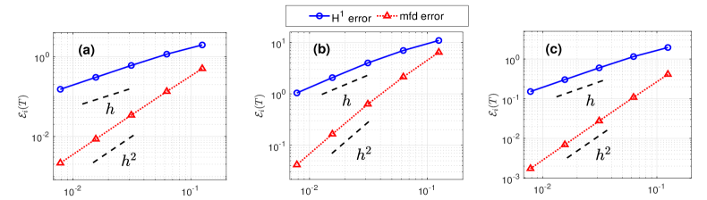
Figure 3: Numerical errors under different norms of the FEM (6.2) at $T=1/4$: (a) Case 1; (b) Case 2; (c) Case 3.

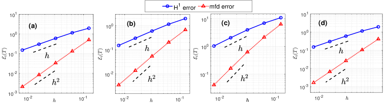
Figure 4: Numerical errors under different norms of the FEM-TM (6.3) at $T=1/4$: (a) Case 1 with $\alpha=1$; (b) Case 1 with $\alpha=0.5$; (c) Case 2 with $\alpha=1$; (d) Case 3 with $\alpha=1$.

The numerical errors of the FEM (6.2) and the FEM-TM (6.3) are presented in Fig 3 and Fig 4, respectively, from which we observe that, for each nonlocal flow with $\mathrm{ind}$ and $\beta$, the solution of (6.2) and (6.3) converge linearly in $L^{\infty}_{t}H^{1}_{x}$, consistent with the theoretical results in Theorems 4.3 and 4.6. Moreover, Fig 4 (a) and (b) illustrate that the scheme (6.3) performs equally well for different choices of $\alpha$. Additionally, we observe that the solution converges quadratically under the manifold distance, which is superior to the theoretical results in Corollary 5.2 (2) and (3).

6.2 Dynamics and evolution of geometric quantities

In this subsection, we utilize the proposed three methods: FDM (6.1), FEM (6.2) and FEM-TM (6.3) to simulate the nonlocal geometric flows. We are mainly concerned with the evolution of the following geometric quantities: perimeter $L(t)$, relative area loss $\Delta A(t)$ and the mesh ratio function $\Psi(t)$ defined as

$$\left.L(t)\right|_{t=t_{k}}=l^{k}_{h},\quad\left.\Delta A(t)\right|_{t=t_{k}}=\frac{A^{k}_{h}-A^{0}_{h}}{A^{0}_{h}},\quad\left.\Psi(t)\right|_{t=t_{k}}=\frac{\max_{j=1,\ldots,N}q^{k}_{j}}{\min_{j=1,\ldots,N}q^{k}_{j}},$$

where $l^{k}_{h}$ and $A^{k}_{h}$ are the perimeter and the area of the polygon determined by $x^{k}_{h}$, respectively, and $q^{k}_{j}=|x^{k}_{j}-x^{k}_{j-1}|$. Note that for the area of an immersed curve, such as the four-leaf rose, it is treated as a signed area. In morphological evolutions, we primarily focus on the following cases:

Case 1: A flower initial curve parametrized by

$$((2+\cos(6\theta))\cos\theta,(2+\cos(6\theta))\sin\theta)^{T},\quad\theta\in[0,2\pi],$$

with the corresponding flow being the AP-CSF with $f(L)=2\pi/L$;

Case 2: A four-leaf rose initial curve, with the corresponding flow being the AP-CSF for nonsimple curve with $f(L)=2\pi\,\mathrm{ind}/L,\mathrm{ind}(\Gamma)=3$;

Case 3: A $4\times 1$ rectangular initial curve with the corresponding flow being a curve flow with area decreasing rate of $\pi$, i.e., $f(L)=(2\pi-\beta)/L$, $\beta=\pi$.

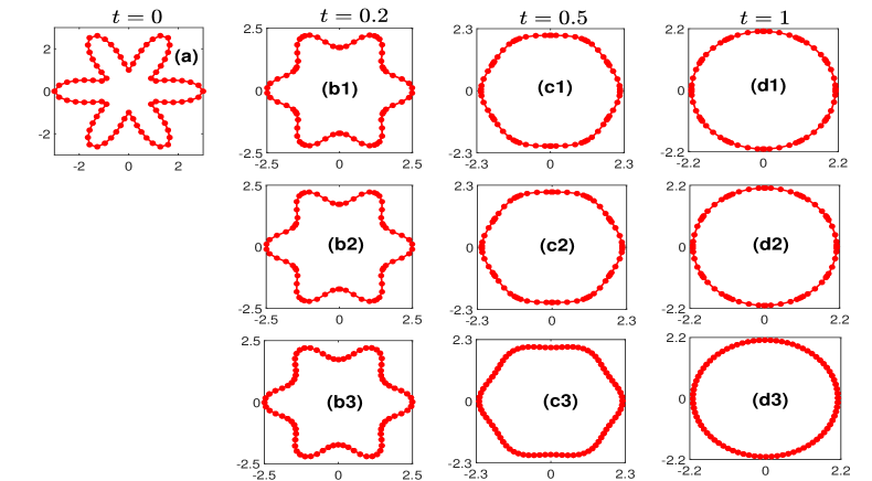
Figure 5: Snapshots of the curve evolution using the FDM (first row), FEM (second row) and FEM-TM (third row) with $\alpha=1$ for Case 1. The parameters are chosen as $N=80$ and $\tau=1/160$.

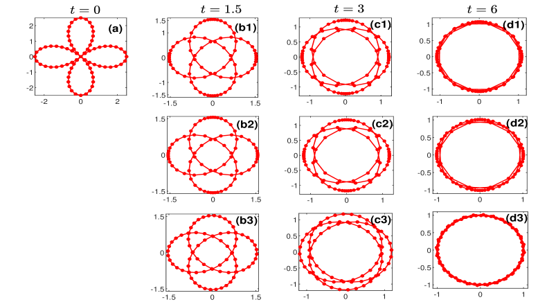
Figure 6: Snapshots of the curve evolution using the FDM (first row), FEM (second row) and FEM-TM (third row) with $\alpha=1$ for Case 2. The parameters are chosen as $N=80$ and $\tau=1/160$.

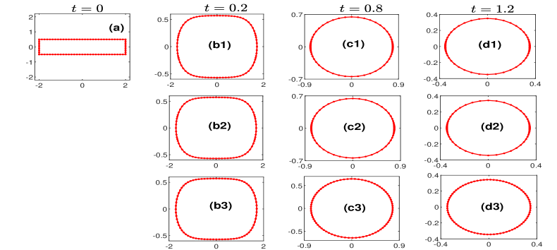
Figure 7: Snapshots of the curve evolution using the FDM (first row), FEM (second row) and FEM-TM (third row) with $\alpha=1$ for Case 3. The parameters are chosen as $N=80$ and $\tau=1/160$.

Figs. 5-8 depict the comparisons of the three schemes through the evolutions of the solution and geometric quantities for the respective three cases. Here we fix the number of nodes $N=80$ and the time step $\tau=1/160$. Based on the observations from Figs. 5-8, we can draw the following conclusions:

1. All of the schemes can evolve the above three cases successfully into their equilibriums, i.e., circle for Case 1, triple circle for Case 2, and a round point for Case 3, which agrees with the theoretical results in [41] (cf. Figs. 5, 6 and 7).

2. For Case 1 and Case 2, the area is conserved numerically up to some precision while the area is decreasing numerically with the rate $\pi$ for Case 3 (cf. Fig. 8 (b)).

3. As demonstrated in Fig. 8 (c), the FEM-TM redistributes the points during the evolution and ultimately achieves the equidistribution property, i.e., $\Psi(t)\rightarrow 1$ as $t\rightarrow+\infty$. This coincides the motivation in Section 4.2. In contrast, the FDM and the FEM fail to preserve good mesh quality during the evolution.

Figure 8: Evolution of the geometric quantities using the FDM, FEM and FEM-TM with $\alpha=1$ for Cases 1-3 is illustrated in the first through third rows, respectively. (a) Perimeter $L(t)$; (b) Relative area loss $\Delta A(t)$; (c) Mesh ratio function $\Psi(t)$. The parameters are chosen as $N=80$ and $\tau=1/160$.

We close this section with a numerical example to demonstrate that the parameter $\alpha$ in the FEM-TM (6.3) signifies the velocity of tangential motions. We conduct simulations for Case 1 using the FEM-TM with varying values $\alpha=0.1,0.5$ and $1$. As depicted in Fig. 9 (c), a smaller $\alpha$ leads to a more effective redistribution of the mesh points. Fig. 9 (b) illustrates that as $\alpha$ approaches $0$, the loss of area becomes greater. This indicates that for a fixed set of computational parameters $N$ and $\tau$, a smaller value of $\alpha$ yields a less accurate simulation, aligning with the findings in Theorem 4.6, wherein the exponential of $\frac{1}{\alpha}$ is involved in the error estimate.

Figure 9: Evolution of geometric quantities using the the FEM-TM with different $\alpha=0.1,0.5,1$ for Case 1. (a) Perimeter $L(t)$; (b) Relative area loss $\Delta A(t)$; (c) Mesh ratio function $\Psi(t)$. The parameters are chosen as $N=80$ and $\tau=1/160$.

7 Conclusions

We developed three distinct semi-discrete schemes for simulating some nonlocal geometric flows involving perimeter and the corresponding error estimates were established. Specifically, the FDM exhibits quadratic convergence in $H^{1}$, whereas the FEM and the FEM-TM are convergent at the first order in $H^{1}$. Furthermore, all three methods demonstrate robust quadratic convergence under manifold distance. Extensive numerical experiments have underscored the superior mesh quality of the FEM-TM compared to FDM and FEM.

It is noteworthy that our proof of the error estimate under manifold distance is not optimal for FEM-TM and FEM. Exploring the possibility of providing a proof of optimal convergence for piecewise linear finite element would be a valuable endeavor.

References

• [1] G. Bai and B. Li. A new approach to the analysis of parametric finite element approximations to mean curvature flow. Found. Comput. Math., doi.org/10.1007/s10208-023-09622-x, 2023.
• [2] E. Bänsch, K. Deckelnick, H. Garcke, and P. Pozzi. Interfaces: modeling, analysis, numerics. Oberwolfach Seminar, Volume 51. Birkhäuser, Springer, 2023.
• [3] E. Bänsch, P. Morin, and R. Nochetto. A finite element method for surface diffusion: The parametric case. J. Comput. Phys., 203:321–343, 2005.
• [4] W. Bao, W. Jiang, and Y. Li. A symmetrized parametric finite element method for anisotropic surface diffusion of closed curves. SIAM J. Numer. Anal., 61(2):617–641., 2023.
• [5] W. Bao and Q. Zhao. A structure-preserving parametric finite element method for surface diffusion. SIAM J. Numer. Anal., 59(5):2775–2799., 2021.
• [6] J. W. Barrett, H. Garcke, and R. Nürnberg. Parametric finite element method approximations of curvature driven interface evolutions. In Andrea Bonito and Ricardo H. Nochetto, editors, Handbook of Numerical Analysis, Volume 21, pages 275–423. Elsevier, 2020.
• [7] L. Bronsard and B. Stoth. Volume-preserving mean curvature flow as a limit of a nonlocal Ginzburg-Landau equation. SIAM J. Math. Anal., 28(4):769–807., 1997.
• [8] A. Chambolle, M. Morini, and M. Ponsiglione. Nonlocal curvature flows. Arch. Ration. Mech. Anal., 218:1263–1329., 2015.
• [9] M. C. Dallaston and S. W. McCue. An accurate numerical scheme for the contraction of a bubble in a Hele-Shaw cell. The ANZIAM Journal, 54:C309–C326, 2012.
• [10] M. C. Dallaston and S. W. McCue. Bubble extinction in Hele-Shaw flow with surface tension and kinetic undercooling regularization. Nonlinearity, 26(6):1639–1665., 2013.
• [11] M. C. Dallaston and S. W. McCue. A curve shortening flow rule for closed embedded plane curves with a prescribed rate of change in enclosed area. Proc. R. Soc. A, 472(2185):20150629, 2016.
• [12] K. Deckelnick and G. Dziuk. On the approximation of the curve shortening flow. Pitman Research Notes in Mathematics Series, pages 100–108., 1995.
• [13] K. Deckelnick, G. Dziuk, and C. M. Elliott. Computation of geometric partial differential equations and mean curvature flow. Acta Numer., 14:139–232., 2005.
• [14] K. Deckelnick and R. Nürnberg. Discrete anisotropic curve shortening flow in higher codimension. arXiv:2310.02138, 2023.
• [15] K. Deckelnick and R. Nürnberg. Discrete hyperbolic curvature flow in the plane. SIAM J. Numer. Anal., 61:1835–1857., 2023.
• [16] K. Deckelnick and R. Nürnberg. A novel finite element approximation of anisotropic curve shortening flow. Interfaces Free Bound., 4:671–708, 2023.
• [17] K. Deckelnick and R. Nürnberg. An unconditionally stable finite element scheme for anisotropic curve shortening flow. Arch. Math., 59:263–274., 2023.
• [18] K. Deckelnick and R. Nürnberg. Finite element schemes with tangential motion for fourth order geometric curve evolutions in arbitrary codimension. arXiv:2402.16799, 2024.
• [19] do Carmo M. P. Differential Geometry of Curves and Surfaces. Dover Publications, Inc., Mineola, NY, 2016.
• [20] B. Duan and B. Li. New artificial tangential motions for parametric finite element approximation of surface evolution. SIAM J. Sci. Comput., 46:A587–A608, 2024.
• [21] G. Dziuk. Discrete anisotropic curve shortening flow. SIAM J. Numer. Anal., 36(6):1808–1830., 1999.
• [22] C. M. Elliott and H. Fritz. On approximations of the curve shortening flow and of the mean curvature flow based on the DeTurck trick. IMA J. Numer. Anal., 37(2):543–603., 2017.
• [23] M. Gage. On an area-preserving evolution equation for plane curves. Contemp. Math., 51:51–62., 1986.
• [24] S. F. Vita I. C. Dolcetta and R. March. Area-preserving curve-shortening flows: from phase separation to image processing. Interfaces Free Bound., 4(4):325–343., 2002.
• [25] L. Jiang and S. Pan. On a non-local curve evolution problem in the plane. Comm. Anal. Geom., 16(1):1–26., 2008.
• [26] W. Jiang, C. Su, and G. Zhang. A convexity-preserving and perimeter-decreasing parametric finite element method for the area-preserving curve shortening flow. SIAM J. Numer. Anal., 61(4):1989–2010., 2023.
• [27] W. Jiang, C. Su, and G. Zhang. A second-order in time, BGN-based parametric finite element method for geometric flows of curves. arXiv:2309.12875., 2023.
• [28] W. Jiang, C. Su, and G. Zhang. Stable BDF time discretization of BGN-based parametric finite element methods for geometric flows. arXiv:2402.03641, 2024.
• [29] U. F. Mayer. A numerical scheme for moving boundary problems that are gradient flows for the area functional. European J. Appl. Math., 11(1):61–80., 2000.
• [30] K. Mikula and D. Ševčovič. Computational and qualitative aspects of evolution of curves driven by curvature and external force. Comput. Vis. Sci., 6(4):211–225., 2004.
• [31] K. Mikula and D. Ševčovič. A direct method for solving an anisotropic mean curvature flow of plane curves with an external force. Math. Methods Appl. Sci., 27(13):1545–1565., 2004.
• [32] L. Pei and Y. Li. A structure-preserving parametric finite element method for area-conserved generalized mean curvature flow. J. Sci. Comput., 96(6):1–21, 2023.
• [33] P. Pozzi and B. Stinner. Convergence of a scheme for elastic flow with tangential mesh movement. ESAIM Math. Model. Numer. Anal., 57(2):445–466, 2023.
• [34] S. J. Ruuth and B. Wetton. A simple scheme for volume-preserving motion by mean curvature. J. Sci. Comput., 19:373–384., 2003.
• [35] G. Sapiro. Geometric Partial Differential Equations and Image Analysis. Cambridge University Press, 2001.
• [36] G. Sapiro and A. Tannenbaum. Area and length preserving geometric invariant scale-spaces. IEEE Trans. Pattern Anal. Mach. Intell., 17:67–72, 1995.
• [37] D. Ševčovič and K. Mikula. Evolution of plane curves driven by a nonlinear function of curvature and anisotropy. SIAM J. Appl. Math., 61(5):1473–1501., 2001.
• [38] D. Tsai and X. Wang. On length-preserving and area-preserving nonlocal flow of convex closed plane curves. Calc. Var. Partial Differential Equations, 54:3603–3622., 2015.
• [39] D. Tsai and X. Wang. The evolution of nonlocal curvature flow arising in a Hele-Shaw problem. SIAM J. Math. Anal., 50(1):1396–1431., 2018.
• [40] T. Ushijima and S. Yazaki. Convergence of a crystalline approximation for an area-preserving motion. J. Comput. Appl. Math., 166(2):427–452., 2004.
• [41] X. Wang and L. Kong. Area-preserving evolution of nonsimple symmetric plane curves. J. Evol. Equ., 14(2):387–401., 2014.
• [42] Q. Zhao, W. Jiang, and W. Bao. An energy-stable parametric finite element method for simulating solid-state dewetting. IMA J. Numer. Anal., 41(3):2026–2055., 2021.