Constructive reachability for linear control problems under conic constraints

Abstract

Motivated by applications requiring sparse or nonnegative controls, we investigate reachability properties of linear infinite-dimensional control problems under conic constraints. Relaxing the problem to convex constraints if the initial cone is not already convex, we provide a constructive approach based on minimising a properly defined dual functional, which covers both the approximate and exact reachability problems. Our main results heavily rely on convex analysis, Fenchel duality and the Fenchel-Rockafellar theorem. As a byproduct, we uncover new sufficient conditions for approximate and exact reachability under convex conic constraints. We also prove that these conditions are in fact necessary. When the constraints are nonconvex, our method leads to sufficient conditions ensuring that the constructed controls fulfill the original constraints, which is in the flavour of bang-bang type properties. We show that our approach encompasses and generalises several works, and we obtain new results for different types of conic constraints and control systems.

1 Introduction

1.1 Control problem and motivations

We let $\displaystyle X$ and $\displaystyle U$ be two Hilbert spaces, $\displaystyle T>0$ be a final time, and denote $\displaystyle E:=L^{2}(0,T;U)$.

We are given an unbounded operator $\displaystyle A:\mathcal{D}(A)\rightarrow X$ generating a $\displaystyle C_{0}$ semigroup on $\displaystyle X$, denoted $\displaystyle(S_{t})_{t\geq 0}$, and $\displaystyle B\in L(U,X)$ a control operator. We then consider the linear control problem

$$\dot{y}=Ay+Bu.$$ (1)

For a constraint set $\displaystyle P\subset U$, a given initial condition $\displaystyle y_{0}\in X$ and a target $\displaystyle y_{f}\in X$, we say that

• $\displaystyle y_{f}$ is approximately reachable from $\displaystyle y_{0}$ in time $\displaystyle T$ under the constraints $\displaystyle P$ if for all $\displaystyle\varepsilon>0$, there exists $\displaystyle u_{\varepsilon}\in E$ such that for a.e. $\displaystyle t\in(0,T)$, $\displaystyle u_{\varepsilon}(t)\in P$ and the corresponding solution to (1) with $\displaystyle y(0)=y_{0}$ and control $\displaystyle u_{\varepsilon}$ satisfies $\displaystyle\|y(T)-y_{f}\|_{X}\leq\varepsilon$.

• $\displaystyle y_{f}$ is exactly reachable from $\displaystyle y_{0}$ in time $\displaystyle T$ under the constraints $\displaystyle P$ if there exists $\displaystyle u\in E$ such that for a.e. $\displaystyle t\in(0,T)$, $\displaystyle u(t)\in P$ and the corresponding solution to (1) with $\displaystyle y(0)=y_{0}$ and control $\displaystyle u$ satisfies $\displaystyle y(T)=y_{f}$.

If there are no constraints, i.e. $\displaystyle P=U$, we will simply write that $\displaystyle y_{f}$ is approximately (resp. exactly) reachable from $\displaystyle y_{0}$ in time $\displaystyle T$.

We are interested in the (constrained) reachability problem when the constraint set $\displaystyle P\subset U$ is a cone, which we will call the constraint cone. In this unbounded setting, it is relevant to distinguish between approximate and exact reachability as these two notions need not coincide, even when $\displaystyle P$ is closed and in finite dimension. An example of this phenomenon in dimension $\displaystyle 2$ is provided in Appendix A.3.

More precisely, we aim at

• deriving necessary and sufficient conditions for approximate and exact reachability,

• developing constructive approaches for the design of controls achieving reachability.

The motivation for unbounded conic constraints mainly comes from two main types of constraints, both of interest for applications. The first type is that of nonnegative constraints, when $\displaystyle X$ is a finite-dimensional space or a functional space (such as $\displaystyle L^{2}$). These are convex conic constraints. The second type is concerned with sparsity constraints. Roughly speaking, these require that, at all times, only a few controls be active. These constraints are not convex and hence prove to be more challenging.

Moreover, as we work with a fixed control time $\displaystyle T$, it is more relevant to consider unbounded constraint sets such as cones, on which optimal control problems with natural quadratic costs can be formulated. On the other hand, bounded constraint sets appear more naturally in minimal time control problems.

1.2 State of the art

Unconstrained reachability and controllability.

The derivation of necessary and sufficient conditions for (unconstrained) reachability associated to linear problems can be traced back to the works of Kalman [15], with a focus on controllability, i.e., reachability results that are independent of the initial state $\displaystyle y_{0}$ and the target $\displaystyle y_{f}$ (and, possibly, of the time $\displaystyle T>0$).

Since then, many such controllability conditions that properly generalise to infinite-dimensional settings have been developed, such as Hautus-type conditions [14, 11], unique continuation properties or observability inequalities [24, 9].

In terms of constructive approaches, which for fixed values of $\displaystyle y_{0},y_{f},T$ should provide a control achieving the target, the so-called Hilbert Uniqueness Method (HUM) developed by Lions has become the method of choice [17, 18]. It is based on minimising a suitably defined functional, and its properties are intimately related to observability inequalities. Lions’ variational technique has in turn inspired works that propose ad hoc functionals for specific constrained control problems [25, 16, 10], or develop sound discretisation methods to derive the corresponding optimal control [7].

Reachability and controllability under constraints.

The problem of constrained control of finite-dimensional linear autonomous systems of the form $\displaystyle\dot{x}=Ax+Bu$ has extensively been studied. The seminal paper [8] provides a general spectral condition on the pair $\displaystyle(A,B)$ to ensure constrained null-controllability, under the hypothesis that this pair is controllable. More recently, the article [20] studied the controllability of linear autonomous systems with positive controls, under the assumption that the Kalman controllability condition holds. In this controllable framework, the authors show that the positivity constraint induces positive minimal control times, and obtain constructive controls through a variational approach.

In infinite dimension, there is no equivalent for the Kalman controllability criterion, and other approaches have been developed to study constrained control problems. The author of [4] develops a variational method which yields necessary and sufficient observability-type conditions for the constrained exact controllability of autonomous linear systems in Hilbert spaces.

Null-controllability conditions for bounded control sets were established in [1] and recovered in [5], with a focus on conservative systems. For the particular case of controls lying in balls, and focusing on parabolic type equations, [6] gives necessary and sufficient conditions for null-controllability.

In all of the above works, the authors develop a variational approach akin to ours, relying on duality in the convex optimisation sense, and obtain constructive controls steering the system to the desired target states. However, it is concerned with general (null) controllability, which leads to strong conditions.

It is worth stressing that, in the presence of constraints, the right notion of controllability becomes unclear. Nonnegative constraints typically may lead to obstructions to controllability: for instance, one has $\displaystyle y_{f}\geq S_{T}y_{0}$ for the heat equation with internal nonnegative constraints, by the parabolic comparison principle [19, 21]. Hence, deriving controllability results (i.e., uniform results with respect to $\displaystyle y_{0}$, $\displaystyle y_{f}$ or both) typically leads to restricting the notion of controllability to a well-defined subset of initial and final targets, as is done in [21].

For general constraints and without specific structural assumptions about the control, the notion of reachability hence becomes more flexible and natural.

Reachability and controllability with conic constraints.

More recently, unbounded constrained controllability or reachability has been the subject of revived interest, motivated by applications where the control should be nonnegative, or more generally, when the constraints on the control are unilateral [19, 20].

Another line of research is that of sparse controls [25, 21]. The former article [25] is focused on approximate and exact reachability for finite-dimensional problems with $\displaystyle m$ controls, with the constraint that at all times, only one control should active. The latter article [21] is concerned with parabolic equations with internal nonnegative controls, and a specific sparsity constraint.

These two works rely on the analysis of a properly defined optimisation problem, through a fine study of a corresponding Fenchel dual problem, in the spirit of the HUM method. Both works are also based on the idea of relaxation which consists of two steps. First, one derives controls within the set of relaxed constraints (obtained by computing the closed convex hull of constraints). Second, one establishes a bang-bang type property that the obtained controls actually take values in the original constraint set.

Main contribution.

The above literature lacks a general framework to investigate constructive reachability in the relevant setting of conic constraints.

Our approach bridges this gap; it subsumes the two works [25, 21] as well as the HUM method, by providing a general recipe for constructive reachability under conic constraints. It accommodates both approximate and exact reachability, thereby yielding sufficient and necessary conditions in the case of convex constraints. The underlying relaxation approach is associated to general sufficient conditions under which optimal controls are bang-bang.

1.3 Notations

To introduce our notations, we let $\displaystyle H$ be a Hilbert space. For clarity, we will use the notation $\displaystyle P$ for cones, $\displaystyle C$ for convex sets, $\displaystyle K$ for general sets. For basic results concerning these notions, we refer, e.g., to [3].

1.3.1 Functions

For a function $\displaystyle f:H\rightarrow\mathopen{]}-\infty,+\infty]$, we let $\displaystyle\mathrm{dom}(f):=\{x\in H,\,f(x)<+\infty\}$ be its domain, and denote $\displaystyle\Gamma_{0}(H)$ the set of functions $\displaystyle H\rightarrow\mathopen{]}-\infty,+\infty]$ that are convex, lower-semicontinuous, and proper (i.e., $\displaystyle\mathrm{dom}(f)\neq\emptyset$).

For a function $\displaystyle f\in\Gamma_{0}(H)$, we let $\displaystyle f^{\ast}$ be its convex conjugate, given by

$$\forall x\in H,\quad f^{\star}(x):=\sup_{y\in H}\,\big{(}\langle x,y\rangle-f(y)\big{)}.$$

We have $\displaystyle f^{\ast}\in\Gamma_{0}(H)$, and Fenchel-Moreau’s theorem states that $\displaystyle(f^{\ast})^{\ast}=f$ for all $\displaystyle f\in\Gamma_{0}(H)$.

For $\displaystyle f\in\Gamma_{0}(H)$ and $\displaystyle x\in H$, we denote

$$\partial f(x):=\{p\in H,\;\forall y\in H,\,f(y)\geq f(x)+\left\langle p,y-x\right\rangle\},$$

the subdifferential set of $\displaystyle f$ at $\displaystyle x$.

For a (non-empty) closed convex set $\displaystyle C\subset H$, we let $\displaystyle\delta_{C}$ be its indicator function, i.e. the function given by $\displaystyle\delta_{C}(x)=0$ if $\displaystyle x\in C$ and $\displaystyle+\infty$ otherwise. We have $\displaystyle\delta_{C}\in\Gamma_{0}(H)$ and we let $\displaystyle\sigma_{C}:=\delta_{C}^{\ast}$ be its support function, which by definition is given by

$$\forall x\in H,\quad\sigma_{C}(x)=\sup_{y\in C}\langle x,y\rangle.$$

Finally, we let $\displaystyle j_{C}$ be the gauge function of $\displaystyle C$, namely

$$\forall x\in H,\quad j_{C}(x):=\inf\{\alpha>0,\;x\in\alpha C\}.$$

See Appendix A.1 for some elementary results concerning gauge functions.

1.3.2 Sets

For a set $\displaystyle K\subset H$, we let

• $\displaystyle\overline{K}$ and $\displaystyle\overline{K}^{w}$ be its (strong) closure and weak closure, respectively,

• $\displaystyle\mathrm{conv}(K)$ be its convex hull,

• $\displaystyle\mathrm{cone}(K)$ be the cone generated by $\displaystyle K$, given by

  $$\mathrm{cone}(K)=\{\lambda p,\;p\in K,\,\lambda>0\}.$$

We also define $\displaystyle\overline{\mathrm{conv}}(K):=\overline{\mathrm{conv}(K)}=\overline{\mathrm{conv}(K)}^{w}$. We recall the caveat that $\displaystyle\mathrm{cone}(K)$ may not be closed even if $\displaystyle K$ is.

For a (non-empty) closed convex set $\displaystyle C\subset H$, we let

• $\displaystyle\mathrm{ext}(C)$ be the set of its extremal points,

• $\displaystyle\mathrm{sing}(C)$ be the set of its singular normal vectors, i.e., vectors $\displaystyle v\in H$ for which the maximum defining $\displaystyle\sigma_{C}(v)$ is reached at multiple points.

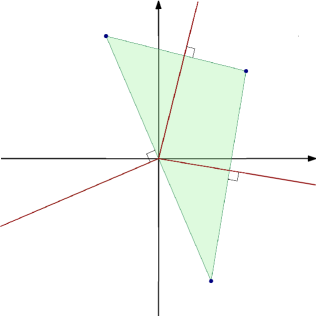
Figure 1: Example of a convex set (in green), with its extreme points (the blue dots), and the cone of its singular normal vectors (the three brown halflines).

We note that $\displaystyle\mathrm{sing}(C)$ is a cone (containing $\displaystyle 0$ as soon as $\displaystyle C$ is not itself reduced to a singleton). For $\displaystyle H_{2}$ another Hilbert space and $\displaystyle B\in L(H,H_{2})$, there holds $\displaystyle x\in\mathrm{sing}(BC)\iff B^{\ast}x\in\mathrm{sing}(C)$.

We recall Milman’s theorem [23]: if $\displaystyle\overline{\mathrm{conv}}{(K)}$ is weakly (respectively strongly) compact, then

$$\mathrm{ext}(\overline{\mathrm{conv}}(K))\subset\overline{K}^{w}\quad\text{resp. }\mathrm{ext}(\overline{\mathrm{conv}}(K))\subset\overline{K}.$$

In particular, $\displaystyle\mathrm{ext}(\overline{\mathrm{conv}}(K))\subset K$ whenever $\displaystyle\overline{\mathrm{conv}}{(K)}$ is weakly (resp. strongly) compact and $\displaystyle K$ weakly (resp. strongly) closed.

Lastly, for a cone $\displaystyle P\subset H$, we let $\displaystyle P^{\circ}$ be its polar cone, i.e., $\displaystyle P^{\circ}:=\{y\in H,\;\forall x\in P,\,\left\langle x,y\right\rangle\leq 0\}$.

1.4 Convex duality framework

1.4.1 Primal and dual optimisation problems

Recall that we are investigating constrained reachability for conic constraints: the constraint set $\displaystyle P\subset U$ is a cone. Our approach will be based on generating the cone $\displaystyle P$ by some prescribed constraint set $\displaystyle\mathcal{U}$, which we call the generating constraint set.

As a result, we will be obtaining controls in $\displaystyle E$ such that, at a.e time $\displaystyle t\in(0,T)$, one can find an amplitude $\displaystyle M(t)\geq 0$ such that $\displaystyle u(t)=M(t)v(t)$ with $\displaystyle v(t)\in\mathcal{U}$. In fact, our approach can also be adapted to build controls whose amplitude does not depend on $\displaystyle t\in(0,T)$, see our discussion in Subsection 1.6.

Throughout, we will always assume that the chosen generating set $\displaystyle\mathcal{U}$ satisfies

$$\mathcal{U} 0\in\mathcal{U}$$ is bounded and . (2)

Given a control system of the form (1), by Duhamel’s formula, one may write $\displaystyle y(T)=S_{T}y_{0}+L_{T}u$ where $\displaystyle L_{T}\in L(E,X)$ is defined by

$$L_{T}u:=\int_{0}^{T}S_{T-t}Bu(t)\,dt.$$

Given $\displaystyle\varepsilon\geq 0$, finding a control $\displaystyle u$ taking values in $\displaystyle P$ steering $\displaystyle y_{0}$ to $\displaystyle\overline{B}(y_{f},\varepsilon)$ in time $\displaystyle T$ is then equivalent to finding $\displaystyle u$ taking values in $\displaystyle P$ such that $\displaystyle L_{T}u\in\overline{B}(\tilde{y}_{T},\varepsilon)$, where

$$\tilde{y}_{T}:=y_{f}-S_{T}y_{0}.$$

Of course, the case $\displaystyle\varepsilon=0$ is concerned with exact reachability since $\displaystyle\overline{B}(\tilde{y}_{T},\varepsilon)=\{\tilde{y}_{T}\}$.

The adjoint $\displaystyle L_{T}^{\ast}\in L(X,E)$ of $\displaystyle L_{T}$ is given for $\displaystyle p_{f}\in X$ by $\displaystyle L_{T}^{\ast}p_{f}(t)=B^{\ast}S_{T-t}^{\ast}p_{f}$, where $\displaystyle(S_{t}^{\ast})_{t\geq 0}$ is the adjoint semigroup, generated by the adjoint operator $\displaystyle A^{\ast}$ to $\displaystyle A$, with domain $\displaystyle\mathcal{D}(A^{\ast})$. In other words, one can write $\displaystyle L_{T}^{\ast}p_{f}(t)=B^{\ast}p(t)$, where $\displaystyle p$ solves the equation

$$\dot{p}+A^{\ast}p=0,\quad p(T)=p_{f}.$$ (3)

Relaxed optimisation problem.

Let $\displaystyle\mathcal{U}\subset U$ be a fixed generating set for $\displaystyle P$ i.e., such that $\displaystyle\mathrm{cone}(\mathcal{U})=\leavevmode\nobreak\ P$, with $\displaystyle\mathcal{U}$ satisfying (2). We define the associated relaxed generating constraint set, and the cone of relaxed constraints it generates,

$$\mathcal{U}_{r}:=\overline{\mathrm{conv}}(\mathcal{U}),\qquad P_{r}:=\mathrm{cone}(\mathcal{U}_{r}).$$

Note that in general, $\displaystyle P_{r}\neq\overline{\mathrm{conv}}(P)$, since the cone generated by a closed set is not necessarily closed. This is summed up by the following diagram:

This schematic highlights that our approach in building $\displaystyle P_{r}$ from $\displaystyle P$ is not canonical. In other words, different choices of generating sets $\displaystyle\mathcal{U}$ may lead to different cones of relaxed contraints $\displaystyle P_{r}$.

Now, we introduce the cost functional given for $\displaystyle u\in E$ by

$$F(u):=\tfrac{1}{2}\int_{0}^{T}j_{\mathcal{U}_{r}}^{2}(u(t))\,dt,$$ (4)

which generalises the quadratic $\displaystyle L^{2}$ norm cost, and depends exclusively on $\displaystyle\mathcal{U}_{r}$. We also denote the set of controls with finite cost

$$L^{2}_{\mathcal{U}_{r}}:=\{u\in E,\;t\mapsto j_{\mathcal{U}_{r}}(u(t))\in L^{2}(0,T)\}=\{u\in E,\;F(u)<+\infty\}.$$

Note that if $\displaystyle u\in L^{2}_{\mathcal{U}_{r}}$, then for a.e. $\displaystyle t\in(0,T)$, $\displaystyle j_{\mathcal{U}_{r}}(u(t))<+\infty$, hence $\displaystyle u(t)\in P_{r}$. In other words, if $\displaystyle u\in L^{2}_{\mathcal{U}_{r}}$, $\displaystyle u$ takes values in the cone of relaxed constraints $\displaystyle P_{r}=\mathrm{cone}(\mathcal{U}_{r})$.

For a given choice of $\displaystyle y_{0},\;y_{f}\in X$, $\displaystyle T>0$ and $\displaystyle\varepsilon\geq 0$, we define the following optimisation problem, in which the conic constraint $\displaystyle u\in P=\operatorname{cone}(\mathcal{U})$ is relaxed to $\displaystyle u\in P_{r}=\operatorname{cone}(\mathcal{U}_{r})$:

$$\inf_{u\in E,\;y(T)\in\overline{B}(\tilde{y}_{T},\varepsilon)}F(u).$$ (5)

By the preceding remarks, if this optimisation problem is not the trivial $\displaystyle+\infty$, then there exists a control $\displaystyle u$ taking values in the cone of relaxed constraints $\displaystyle\mathrm{cone}(\mathcal{U}_{r})$ steering $\displaystyle y_{0}$ to $\displaystyle\overline{B}(y_{f},\varepsilon)$ in time $\displaystyle T>0$.

Duality for the relaxed problem.

We show (see Proposition 3.2) that $\displaystyle F$ is in $\displaystyle\Gamma_{0}(E)$ with, for all $\displaystyle p\in E$,

$$F^{\ast}(p)=\tfrac{1}{2}\int_{0}^{T}\sigma_{\mathcal{U}_{r}}^{2}(p(t))\,dt,$$ (6)

and that this function takes finite values on the whole of $\displaystyle E$, namely $\displaystyle\mathrm{dom}(F^{\ast})=E$. Finally, for all $\displaystyle\varepsilon\geq 0$, we let

$$\forall p_{f}\in X,\quad J_{\varepsilon}(p_{f}):=F^{\ast}(L_{T}^{\ast}p_{f})-\langle\tilde{y}_{T},p_{f}\rangle_{X}+\varepsilon\|p_{f}\|_{X},$$ (7)

and consider the associated so-called dual problem

$$\inf_{p_{f}\in X}J_{\varepsilon}(p_{f}).$$ (8)

The optimisation problem (5) is correspondingly called the primal problem.

1.4.2 Optimality conditions

For a given choice of $\displaystyle\varepsilon\geq 0$, $\displaystyle y_{0},y_{f}\in X$, $\displaystyle T>0$, the functional $\displaystyle J_{\varepsilon}$ may or may not admit a minimiser over $\displaystyle X$. If it does, we will see that the primal optimisation problem (5) is not the trivial $\displaystyle+\infty$. More precisely, if $\displaystyle p_{f}^{\star}$ is a minimiser, all optimal controls must satisfy $\displaystyle u\in\partial F^{\ast}(L_{T}^{\ast}p_{f}^{\star})$. Denoting $\displaystyle q^{\star}:=L_{T}^{\ast}p_{f}^{\star}$, we will show that this corresponds to

$$\text{for a.e. }t\in(0,T),\quad u(t)\in\sigma_{\mathcal{U}_{r}}(q^{\star}(t))\,\partial\sigma_{\mathcal{U}_{r}}(q^{\star}(t))=\sigma_{\mathcal{U}_{r}}(q^{\star}(t))\,\operatorname*{arg\,max}_{v\in\mathcal{U}_{r}}\;\langle q^{\star}(t),v\rangle_{U}.$$ (9)

Our method is a natural extension of the HUM method (a connection on which we elaborate in Section 2.1). It yields controls with a varying amplitude: $\displaystyle j_{\mathcal{U}_{r}}(u(t))$ is time dependent.

Uniqueness.

These formulae will not always define a unique control, but we will see that at least one control satisfying (9) is an optimal control for (5). In fact, they will define a unique control if and only if

$$L_{T}^{\ast}p_{f}^{\star}(t)\notin\mathrm{sing}(\mathcal{U}_{r})\cap(P_{r}^{\circ})^{c}\text{ for a.e. }t\in(0,T).$$ (H)

This amounts to requiring $\displaystyle L_{T}^{\ast}p_{f}^{\star}$ to "avoid" the cone of singular normal vectors to $\displaystyle\mathcal{U}_{r}$, intersected with the complement of the polar cone $\displaystyle P_{r}^{\circ}$.

Extremality.

The optimal control above is a relaxation of the original constrained problem, in which the controls are required to take values in the cone of relaxed constraints $\displaystyle P_{r}$. In order to obtain controls satisfying the original constraints given by the cone $\displaystyle P$ upon solving the relaxed problem, a final hypothesis will be of interest:

$$\mathrm{ext}(\mathcal{U}_{r})\subset\mathcal{U}.$$ (E)

Since $\displaystyle\mathcal{U}$ is assumed to be bounded, so is the closed convex set $\displaystyle\mathcal{U}_{r}$; hence the latter set is weakly compact. As a result, an application of Milman’s theorem with either the strong or the weak topology shows that (E) holds true as soon as either one of the following hypotheses holds

• $\displaystyle\mathcal{U}$ is weakly closed,

• $\displaystyle\mathcal{U}_{r}$ is strongly compact and $\displaystyle\mathcal{U}$ is strongly closed.

1.5 Main results

Our two main theorems 1.1 and 1.2 below are concerned with approximate and exact reachability, respectively. Most results are obtained by studying the dual functional (7), whether for all $\displaystyle\varepsilon>0$ or for $\displaystyle\varepsilon=0$. In fact, the sufficiency of our sufficient conditions for reachability (10) and (12) stem from that analysis, but the necessity is proved by independent arguments.

Finally, recall the basic assumption (2) about the generating constraint set, an assumption that underlies all the presented results.

1.5.1 Approximate reachability

First, we consider the case of approximate reachability. In terms of constructive approaches, this corresponds to studying the dual functionals (7) for all $\displaystyle\varepsilon>0$.

Theorem 1.1.

The state $\displaystyle y_{f}$ is approximately reachable from $\displaystyle y_{0}$ in time $\displaystyle T>0$ under the cone of relaxed constraints $\displaystyle P_{r}=\mathrm{cone}(\mathcal{U}_{r})$ if and only if

$$\forall p_{f}\in X,\quad F^{\ast}(L_{T}^{\ast}p_{f})=0\;\implies\;\left\langle\tilde{y}_{T},p_{f}\right\rangle_{X}\leq 0.$$ (10)

Now assume that the latter condition holds. Then $\displaystyle J_{\varepsilon}$ admits a unique minimiser $\displaystyle p_{f}^{\star}$ for any value of $\displaystyle\varepsilon>0$, and at least one control $\displaystyle u\in\partial F^{\ast}(L_{T}^{\ast}p_{f}^{\star})$ steers the solution of (1) from $\displaystyle y_{0}$ to the ball $\displaystyle\overline{B}(y_{f},\varepsilon)$ in time $\displaystyle T$. Furthermore,

• there exists a unique such control if and only if (H) holds,

• if in addition (E) holds, the unique control takes values in the original cone $\displaystyle P=\mathrm{cone}(\mathcal{U})$.

It might be surprising that condition (10) is equivalent to an approximate reachability condition regarding $\displaystyle P_{r}$, since $\displaystyle F^{\ast}$ depends on $\displaystyle\mathcal{U}_{r}$. We provide yet another equivalent condition that indeed explicitly depends only on the cone of relaxed constraints $\displaystyle P_{r}$.

Lemma 1.1.

Let $\displaystyle P_{r}=\mathrm{cone}(\mathcal{U}_{r})$. Then (10) is equivalent to

$$\forall p_{f}\in X,\quad\left(\text{for a.e. }t\in(0,T),\quad L_{T}^{\ast}p_{f}(t)\in P_{r}^{\circ}\right)\quad\implies\quad\langle\tilde{y}_{T},p_{f}\rangle_{X}\leq 0.$$ (11)

1.5.2 Exact reachability

Second, we consider a necessary and sufficient condition for exact reachability, which leads to a constructive control under some additional technical assumptions. In terms of constructive approaches, this corresponds to studying the dual functional (7) for $\displaystyle\varepsilon=0$. We will be interested in the quantity

$$c^{\star}:=\inf\left\{c\geq 0,\;\forall p_{f}\in X,\;\left\langle\tilde{y}_{T},p_{f}\right\rangle_{X}\leq c\,F^{\ast}(L_{T}^{\ast}p_{f})^{1/2}\right\}=\sup_{\|p_{f}\|_{X}=1}\frac{\left\langle\tilde{y}_{T},p_{f}\right\rangle_{X}}{F^{\ast}(L_{T}^{\ast}p_{f})^{1/2}},$$

with the convention $\displaystyle 0/0=0$, $\displaystyle\alpha/0=+\infty$ for $\displaystyle\alpha>0$. Note that $\displaystyle c^{\star}\in[0,+\infty]$, and $\displaystyle c^{\star}\in(0,+\infty]$ if and only if $\displaystyle\tilde{y}_{T}\neq 0$.

In the case of exact reachability, we are led to specify some additional time-regularity controls may/should have, in the form $\displaystyle u\in L^{2}_{\mathcal{U}_{r}}$. In this case, we will say that $\displaystyle y_{f}$ is exactly reachable from $\displaystyle y_{0}$ in time $\displaystyle T$ under the constraints $\displaystyle P$ (or $\displaystyle P_{r}$) with controls in $\displaystyle L^{2}_{\mathcal{U}_{r}}$.

Theorem 1.2.

The state $\displaystyle y_{f}$ is exactly reachable from $\displaystyle y_{0}$ in time $\displaystyle T>0$ under the cone of relaxed constraints $\displaystyle P_{r}=\mathrm{cone}(\mathcal{U}_{r})$ with controls in $\displaystyle L^{2}_{\mathcal{U}_{r}}$ if and only if

$$\exists c>0,\;\forall p_{f}\in X,\quad\left\langle\tilde{y}_{T},p_{f}\right\rangle_{X}\leq c\,F^{\ast}(L_{T}^{\ast}p_{f})^{1/2}.$$ (12)

Now assume that the latter condition holds, i.e., $\displaystyle c^{\star}<+\infty$. Then $\displaystyle J_{0}$ admits a minimiser if and only if $\displaystyle c^{\star}$ is attained, and if so for any such minimiser $\displaystyle p_{f}^{\star}$, at least one control $\displaystyle u\in\partial F^{\ast}(L_{T}^{\ast}p_{f}^{\star})$ steers the solution of (1) from $\displaystyle y_{0}$ to $\displaystyle y_{f}$ in time $\displaystyle T$. Furthermore,

• there exists a unique such control if and only if (H) holds,

• if in addition (E) holds, the unique control takes values in the original cone $\displaystyle P=\mathrm{cone}(\mathcal{U})$.

Contrarily to the case of approximate reachability, we must consider the additional information that controls are in $\displaystyle L^{2}_{\mathcal{U}_{r}}$. Let us give one general sufficient condition making this condition superfluous.

If $\displaystyle\mathcal{U}_{r}$ (which is a closed, bounded and convex set) is such that $\displaystyle 0$ is in the interior of $\displaystyle\mathcal{U}_{r}$ relative to the cone it generates, i.e., if

$$\exists\delta>0,\quad\mathrm{cone}(\mathcal{U}_{r})\cap\overline{B}(0,\delta)\subset\mathcal{U}_{r},$$ (13)

then it is easily seen that $\displaystyle j_{\mathcal{U}_{r}}(u)\leq\delta^{-1}\|u\|_{U}$ for all $\displaystyle u\in U$. As a result, if $\displaystyle\mathcal{U}_{r}$ satisfies (13), then $\displaystyle L^{2}_{\mathcal{U}_{r}}=E$ so that the additional regularity requirement that controls be in $\displaystyle L^{2}_{\mathcal{U}_{r}}$ may safely be removed. We also note that under (13), $\displaystyle P_{r}=\mathrm{cone}(\mathcal{U}_{r})$ is closed, see Appendix A.1.

1.5.3 Consequences

Let us now explain the implications these theorems have, first when the chosen set $\displaystyle\mathcal{U}$ to generate the cone $\displaystyle P$ is convex and closed, second when this assumption is dropped.

Convex closed case.

First, assume that $\displaystyle\mathcal{U}$ is convex and closed, in which case relaxation is unnecessary. Hence, $\displaystyle\mathcal{U}_{r}=\mathcal{U}$ and $\displaystyle P_{r}=\mathrm{cone}(\mathcal{U}_{r})=\mathrm{cone}(\mathcal{U})=P$, making the assumption (E) true (since $\displaystyle\mathcal{U}$ is then weakly closed) but pointless.

In this case, Theorem 1.1 shows that whenever $\displaystyle y_{f}$ is approximately reachable from $\displaystyle y_{0}$ in time $\displaystyle T>0$ under the constraints $\displaystyle P=P_{r}$, our method provides a constructive way to obtain controls achieving approximate reachability, provided that (H) holds.

Theorem 1.2 shows that whenever $\displaystyle y_{f}$ is exactly reachable from $\displaystyle y_{0}$ in time $\displaystyle T>0$ under the constraints $\displaystyle P=P_{r}$ with controls in $\displaystyle L^{2}_{\mathcal{U}_{r}}=L^{2}_{\mathcal{U}}$, our method provides a constructive way to obtain controls achieving exact reachability, provided that $\displaystyle c^{\star}$ is attained and (H) holds.

General case.

When $\displaystyle\mathcal{U}$ is no longer assumed to be convex and closed, Theorem 1.1 and Theorem 1.2 yield new reachability results in the following sense.

If $\displaystyle y_{f}$ is approximately reachable from $\displaystyle y_{0}$ in time $\displaystyle T>0$ with controls under the cone of relaxed constraints $\displaystyle P_{r}=\mathrm{cone}(\mathcal{U}_{r})$, then $\displaystyle y_{f}$ is also approximately reachable from $\displaystyle y_{0}$ to $\displaystyle y_{f}$ in time $\displaystyle T>0$ under the original constraint cone $\displaystyle P=\mathrm{cone}(\mathcal{U})$, provided that (H) and (E) hold. Furthermore, our method provides a constructive way to build controls achieving approximate reachability.

If $\displaystyle y_{f}$ is exactly reachable from $\displaystyle y_{0}$ in time $\displaystyle T>0$ with controls under the cone of relaxed constraints $\displaystyle P_{r}=\mathrm{cone}(\mathcal{U}_{r})$ with controls in $\displaystyle L^{2}_{\mathcal{U}_{r}}$, then $\displaystyle y_{f}$ is also exactly reachable from $\displaystyle y_{0}$ to $\displaystyle y_{f}$ in time $\displaystyle T>0$ under the original constraint cone $\displaystyle P=\mathrm{cone}(\mathcal{U})$, provided that $\displaystyle c^{\star}$ is attained and that (H) and (E) hold. Furthermore, our method provides a constructive way to build controls achieving exact reachability.

The bang-bang principle.

Our results bear a strong connexion to the so-called bang-bang principle. The bang-bang principle is a property that many control systems satisfy, which can be stated as follows

$$R^{T}_{K}(y_{0})=R^{T}_{\operatorname{ext}(K)}(y_{0}),$$

where the notation $\displaystyle R_{K}^{T}(y_{0})$ stands for the reachable set from $\displaystyle y_{0}$ in time $\displaystyle T$, under the constraints given by the set $\displaystyle K$. The above principle hence means that any state that can be reached in time $\displaystyle T$, from a given initial state $\displaystyle y_{0}$, with controls in a convex compact set $\displaystyle K$, can also be reached with controls in the set of extremal points of $\displaystyle K$.

It also exists in the weaker form

$$R^{T}_{K}(y_{0})=\overline{R^{T}_{\operatorname{ext}(K)}(y_{0})}^{w},$$

for weakly compact convex sets $\displaystyle K$. We refer to [13] for more details.

An important difference is that our constraint sets are not bounded, as they are cones, but we do consider generating sets which are bounded. Relaxing these constraint sets to their convex hulls allows us to work with a convex optimization framework, in which we recover, under certain general conditions, a form of bang-bang principle.

Condition (H).

Since the central condition (H) may not be straightforward to check as one has little information about $\displaystyle p_{f}^{\star}$, one may replace it with the following weaker condition that no longer depends on $\displaystyle\varepsilon\geq 0$, $\displaystyle y_{0}$, $\displaystyle y_{f}$ and $\displaystyle T>0$:

$$\forall p_{f}\neq 0,\quad B^{\ast}S_{t}^{\ast}p_{f}\notin\mathrm{sing}(\mathcal{U}_{r})\cap(P_{r}^{\circ})^{c}\text{ for a.e. }t>0. \widetilde{\text{H}}$$ ()

Of course, ($\displaystyle\widetilde{\text{H}}$) implies  (H). In order to discuss the above conditions, we give the following useful result when it comes to proving that the adjoint trajectory does not spend time within a given set.

For a vector $\displaystyle b\in X$, we let $\displaystyle\ell(b)$ be the largest integer such that $\displaystyle b\in\mathcal{D}(A^{j})$, with the convention $\displaystyle\ell(b)=+\infty$ if $\displaystyle b\in\mathcal{D}(A^{j})$ for all $\displaystyle j\in\mathbb{N}$.

Proposition 1.1.

Let $\displaystyle K\subset X$ be any set, and assume that

• the semigroup $\displaystyle(S_{t}^{\ast})$ is injective,

• $$\big{(}\mathrm{Ran}\big{\{}A^{j}b,\;b\in K^{\perp},\,0\leq j\leq\ell(b)\big{\}}\big{)}^{\perp}=\{0\}.$$

Then the set $\displaystyle\{t\geq 0,\,S_{t}^{\ast}p_{f}\in K\}$ is of measure $\displaystyle 0$ for any $\displaystyle p_{f}\neq 0$.

The proof of Proposition 1.1 is given in Appendix A.2.

Recall that $\displaystyle B^{\ast}q\in\mathrm{sing}(\mathcal{U}_{r})$ if and only if $\displaystyle q\in\mathrm{sing}(B\mathcal{U}_{r})$, and note that $\displaystyle B^{\ast}q\in(P_{r}^{\circ})^{c}$ if and only if $\displaystyle q\in((BP_{r})^{\circ})^{c}$. Hence, one can in practice try and apply Proposition 1.1 to $\displaystyle K=\mathrm{sing}(B\,\mathcal{U}_{r})\cap((BP_{r})^{\circ})^{c}$ to obtain ($\displaystyle\widetilde{\text{H}}$). However, it is important to note that Proposition 1.1 only sees the closure of the subspace spanned by $\displaystyle K$, in the sense that $\displaystyle K$ satisfies the required hypotheses if and only if $\displaystyle\overline{\mathrm{Ran}(K)}$ does, since $\displaystyle\overline{\mathrm{Ran}(K)}$ and $\displaystyle K$ have the same orthogonal complement. As a result, it will usually be more appropriate to use Proposition 1.1 to subcones that constitute the cone $\displaystyle\mathrm{sing}(B\mathcal{U}_{r})\cap((BP_{r})^{\circ})^{c}$.

In practical cases and in finite dimension, there will indeed typically be finitely many such subcones; see Subsection 2.2 for an example.

1.6 Extensions and perspectives

Alternative cost.

It would be possible to consider a slightly different cost than (4), namely

$$F(u):=\tfrac{1}{2}\sup_{t\in(0,T)}j_{\mathcal{U}_{r}}^{2}(u(t)).$$ (14)

which would lead to the dual functional $\displaystyle J_{\varepsilon}$ as before but with $\displaystyle F^{\ast}$ given by

$$F^{\ast}(p)=\tfrac{1}{2}\left(\int_{0}^{T}\sigma_{\mathcal{U}_{r}}(p(t))\,dt\right)^{2}.$$ (15)

One advantage is that one would obtain controls with a fixed amplitude rather than a time-varying one, which can be an interesting feature for applications. In fact, this is done in [21] for a specific control problem.

However, this alternative cost would lead to several adjustments; in particular, the more natural functional setting for generalising all our results to (15) would be $\displaystyle L^{\infty}(0,T;U)$, which has a less natural dual structure than $\displaystyle E=L^{2}(0,T;U)$. In order to lighten our presentation, we have chosen not to do so.

Open questions.

In the convex case, our variational method allowed us to derive sufficient conditions for approximate or exact reachability in cone. We have further proved that these conditions happen to be necessary, by other means.

In the non-convex case, relaxation yields a set of sufficient conditions for approximate or exact reachability in nonconvex cones. This leaves open the question of the necessity of these conditions.

Accordingly, studying the necessity of these conditions will allow for a more detailed picture of the bang-bang principle in infinite dimensions, with undounded constraints. Indeed, finding counterexamples, or proving that these conditions are necessary, will provide an in-depth understanding of failures of the bang-bang principle in infinite dimension.

Outline of the paper.

Our article is split into two parts. The purpose of Section 2 is to apply our method to various examples, which leads to the generalisation of previous works as well as to new results. Then, Section 3 compiles the proofs of all our results, building upon the Fenchel-Rockafellar theorem.

2 Examples and applications

We discuss the application of our method to four examples.

• we show that the HUM method is a particular case of our methodology.

• we analyse a toy example in small dimension with non-convex constraints. We explain in full detail how to properly follow the different steps underlying our method.

• we study abstract general finite-dimensional control problems under the $\displaystyle k$-sparsity constraints. This generalises an approach developed in [25] for $\displaystyle k=1$.

• we discuss approximate reachability for control problems in $\displaystyle L^{2}(\Omega)$. First, we consider nonnegativity constraints and then proceed to adding specific sparsity constraints. We recover the result of [21] regarding the on-off shape control of parabolic equations, with the subtle difference that controllers have time-varying amplitude.

2.1 Unconstrained case

2.1.1 HUM method

We here assume that $\displaystyle\mathcal{U}$ is the unit ball $\displaystyle\{u\in U,\;\|u\|_{U}\leq 1\}$, which obviously falls in the convex case with $\displaystyle\mathcal{U}_{r}=\mathcal{U}$.

Then the cone $\displaystyle\mathrm{cone}(\mathcal{U}_{r})=P_{r}=P=\mathrm{cone}(\mathcal{U})$ is the whole of $\displaystyle U$: we are in the unconstrained case. In this setting, there are numerous sufficient conditions for approximate (resp. exact) controllability to hold, yielding approximate (resp. exact) reachability independently of $\displaystyle y_{0}$, $\displaystyle y_{f}$ and, possibly, $\displaystyle T>0$. In this case, we find $\displaystyle\sigma_{\mathcal{U}}(u)=j_{\mathcal{U}}(u)=\|u\|_{U}$, meaning that $\displaystyle F^{\ast}(p)=\tfrac{1}{2}\|p\|_{E}^{2}$, hence the functional $\displaystyle J_{\varepsilon}$ boils down to

$$\displaystyle J_{\varepsilon}(p_{f})=\tfrac{1}{2}\int_{0}^{T}\|L_{T}^{\ast}p_{f}(t)\|_{U}^{2}\,dt-\langle\tilde{y}_{T},p_{f}\rangle_{X}+\varepsilon\|p_{f}\|_{X}=\tfrac{1}{2}\|L_{T}^{\ast}p_{f}\|_{E}^{2}-\langle\tilde{y}_{T},p_{f}\rangle_{X}+\varepsilon\|p_{f}\|_{X}$$ (16)

and the corresponding optimisation problem is given by

$$\inf_{u\in E,\;y(T)\in\overline{B}(\tilde{y}_{T},\varepsilon)}\tfrac{1}{2}\int_{0}^{T}\|u(t)\|_{X}^{2}\,dt=\inf_{u\in E,\;y(T)\in\overline{B}(\tilde{y}_{T},\varepsilon)}\tfrac{1}{2}\|u\|_{E}^{2}.$$

For $\displaystyle\varepsilon=0$, we recover the functional underlying the so-called Hilbert Uniqueness Method, introduced by Lions in [17]. For $\displaystyle\varepsilon>0$, we recover the functional introduced by Lions in [18] to study approximate controllability.

Whenever a dual optimal variable exists, it gives rise to a unique control through (9), since the latter equation then amounts to $\displaystyle u^{\star}=L_{T}^{\ast}p_{f}^{\star}$.

2.1.2 Exact controllability

As is well known, exact controllability at time $\displaystyle T$ (i.e., exact reachability for any $\displaystyle y_{0},y_{f}\in X$ in time $\displaystyle T$) is equivalent to the observability inequality:

$$\exists C>0,\,\forall p_{f}\in X,\quad\|p_{f}\|_{X}^{2}\leq C^{2}\|L_{T}^{\ast}p_{f}\|_{E}^{2}$$ (17)

Furthermore, it is also well known that one may then achieve exact controllability by minimising the functional $\displaystyle J_{0}$, that is, the dual functional attains its minimum. Indeed, it is easily seen to be coercive in this case.

Let us explain how our framework recovers this case as well: we have $\displaystyle c^{\star}<+\infty$ and $\displaystyle c^{\star}$ is attained, whatever the choice of $\displaystyle y_{0},y_{f}$ in $\displaystyle X$.

Proposition 2.1.

Let $\displaystyle T>0$ be fixed, and assume that (17) holds. Then whatever $\displaystyle y_{0}$, $\displaystyle y_{f}$ in $\displaystyle X$, $\displaystyle c^{\star}<+\infty$ and it is attained.

Proof.

We let $\displaystyle y_{0}$, $\displaystyle y_{f}$ be fixed in $\displaystyle X$. The first statement is readily obtained by applying the Cauchy-Schwarz inequality:

$$\forall p_{f}\in X,\quad\langle\tilde{y}_{T},p_{f}\rangle_{X}\leq\|\tilde{y}_{T}\|_{X}\|p_{f}\|_{X}\leq C\|\tilde{y}_{T}\|_{X}\|L_{T}^{\ast}p_{f}\|_{E}=\sqrt{2}C\|\tilde{y}_{T}\|_{X}F^{\ast}(L_{T}^{\ast}p_{f})^{1/2},$$

this shows that $\displaystyle c^{\star}\leq\sqrt{2}C\|\tilde{y}_{T}\|_{X}<+\infty$.

Now let us prove that $\displaystyle c^{\star}$ is attained. The case $\displaystyle\tilde{y}_{T}=0$ (which corresponds to $\displaystyle S_{T}y_{0}=y_{f}$ or, equivalently, to $\displaystyle c^{\star}=0$) is obvious.

In the interesting case where $\displaystyle\tilde{y}_{T}\neq 0$ or equivalently $\displaystyle c^{\star}>0$, let $\displaystyle(p_{f}^{n})$, $\displaystyle\|p_{f}^{n}\|_{X}=1$ be a maximising sequence, i.e., $\displaystyle\tfrac{\langle\tilde{y}_{T},p_{f}^{n}\rangle_{X}}{\|L_{T}^{\ast}p_{f}^{n}\|_{E}}$ converges to $\displaystyle c^{\star}$. Upon extraction, we may assume that $\displaystyle p_{f}^{n}\rightharpoonup p_{f}$ in $\displaystyle X$. The numerator hence converges, and we must have $\displaystyle\langle\tilde{y}_{T},p_{f}\rangle_{X}\geq 0$ for the quotient to converge to a positive value. Now in view of (17), we have $\displaystyle\|L_{T}^{\ast}p_{f}^{n}\|_{E}\geq C^{-1}\|p_{f}^{n}\|_{X}=C^{-1}$, hence the denominator is bounded away from $\displaystyle 0$. This proves that the numerator actually has to converge to a positive value, namely $\displaystyle\langle\tilde{y}_{T},p_{f}\rangle_{X}>0$. In particular, we have $\displaystyle p_{f}\neq 0$ and hence, again by (17), $\displaystyle L_{T}^{\ast}p_{f}\neq 0$.

By weak lower semicontinuity of the norm and given that $\displaystyle L_{T}^{\ast}p_{f}^{n}\rightharpoonup L_{T}^{\ast}p_{f}$ in $\displaystyle E$, we find

$$\frac{\langle\tilde{y}_{T},p_{f}\rangle_{X}}{\|L_{T}^{\ast}p_{f}\|_{E}}\geq\limsup\frac{\langle\tilde{y}_{T},p_{f}^{n}\rangle_{X}}{\|L_{T}^{\ast}p_{f}^{n}\|_{E}}=c^{\star},$$

showing that $\displaystyle p_{f}$ (or more precisely, $\displaystyle\tfrac{p_{f}}{\|p_{f}\|_{X}}$) reaches the supremum $\displaystyle c^{\star}$.

∎

2.2 A finite-dimensional example

2.2.1 Setting

We are in the case where $\displaystyle X=\mathbb{R}^{3}$, $\displaystyle U=\mathbb{R}^{2}$, with

$$A=\begin{pmatrix}1&2&0\\ 1&-1&2\\ 1&1&-1\end{pmatrix},\qquad B=\begin{pmatrix}1&0\\ -1&1\\ 0&0\\ \end{pmatrix}$$ (18)

It is easily seen that the pair $\displaystyle(A,B)$ satifies Kalman’s rank condition. Hence for any $\displaystyle y_{0},y_{f}\in X$ and $\displaystyle T>0$, $\displaystyle y_{f}$ is exactly reachable from $\displaystyle y_{0}$ in time $\displaystyle T$ (in the absence of constraints).

Now consider the following cone as a constraint set

$$P:=\{(u_{1},u_{2})\in\mathbb{R}^{2},\;u_{1}\geq 0\text{ or }u_{1}\leq 0,\;u_{2}=0\}.$$ (19)

We generate the cone $\displaystyle P$ by intersecting with the unit ball of $\displaystyle\mathbb{R}^{2}$, that is, we set

$$\mathcal{U}:=P\cap\overline{B}(0,1).$$

The resulting set is not convex, hence we form the relaxed constraint set $\displaystyle\mathcal{U}_{r}$, which is given by

$$\mathcal{U}_{r}=\left(\overline{B}(0,1)\cap\{(u_{1},u_{2})\in\mathbb{R}^{2},\,u_{1}\geq 0\}\right)\cup\left(\overline{B}_{1}(0,1)\cap\{(u_{1},u_{2})\in\mathbb{R}^{2},\,u_{1}\leq 0\}\right),$$

where we use the shorthand notation $\displaystyle\overline{B}_{p}(0,1)$ for the unit ball associated to the $\displaystyle\ell^{p}$ norm.

Note that the cone $\displaystyle P_{r}$ generated by $\displaystyle\mathcal{U}_{r}$ is the whole of $\displaystyle\mathbb{R}^{2}$. Hence, for any $\displaystyle y_{0},y_{f}\in X$ and $\displaystyle T>0$, $\displaystyle y_{f}$ is exactly reachable from $\displaystyle y_{0}$ in time $\displaystyle T$ under the constraints $\displaystyle P_{r}$, since this amounts to not having constraints at all. These sets are illustrated by Figure 2.

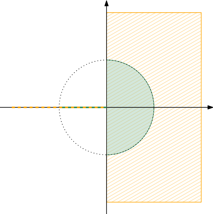
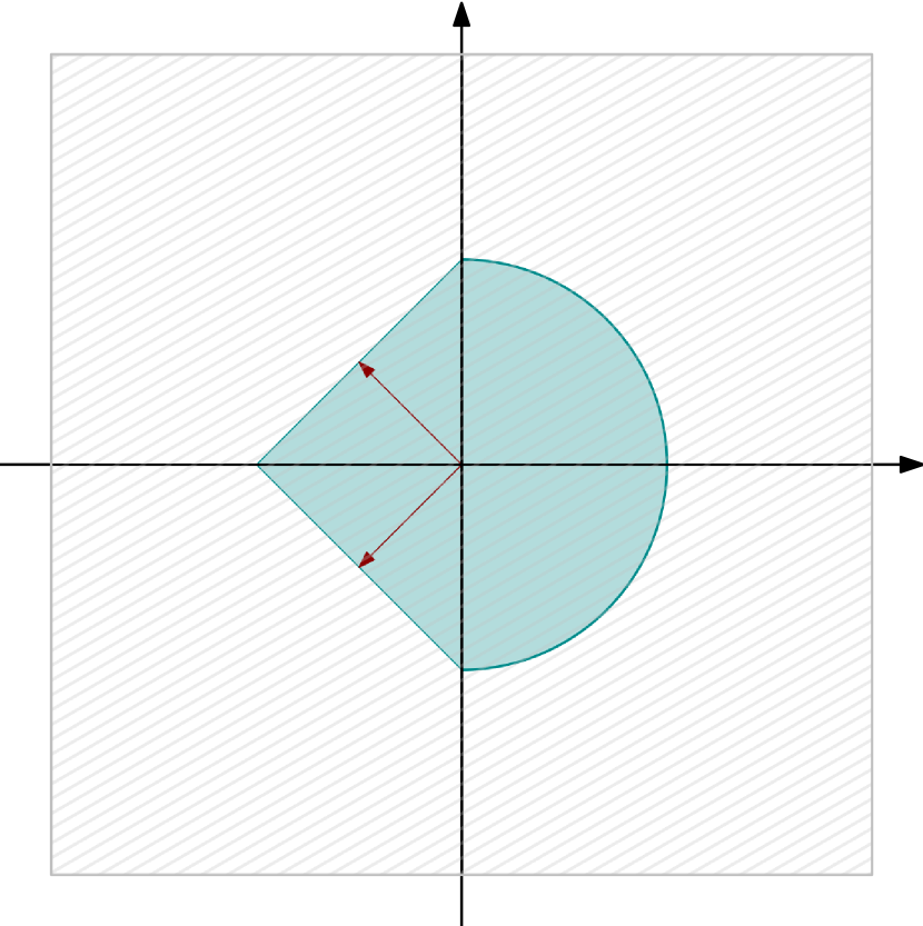
Figure 2: The left figure shows the constraint cone $\displaystyle P$ (hatched pale orange area) with the set $\displaystyle\mathcal{U}$ chosen to generate it (in green). The right figure shows the relaxed constraint set $\displaystyle\mathcal{U}_{r}$ (in cyan). The cone $\displaystyle P_{r}$ it generates is the whole of $\displaystyle\mathbb{R}^{2}$ (the hatched area in gray). The two vectors (in magenta) generate the cone of singular vectors $\displaystyle\mathrm{sing}(\mathcal{U}_{r})$.

2.2.2 Functional and optimality conditions

We focus on on exact reachability, hence we set $\displaystyle\varepsilon=0$. First, we compute the gauge and support functions of $\displaystyle\mathcal{U}_{r}$:

$$\forall u\in\mathbb{R}^{2},\qquad j_{\mathcal{U}_{r}}(u)=\begin{cases}\|u\|_{1}&\text{ if }u_{1}\leq 0\\ \|u\|&\text{ if }u_{1}>0\\ \end{cases},\qquad\sigma_{\mathcal{U}_{r}}(u)=\begin{cases}\|u\|_{\infty}&\text{ if }u_{1}\leq 0\\ \|u\|&\text{ if }u_{1}>0\\ \end{cases}.$$

These computations being made, they completely define the primal and dual optimisation problems. Now let us make the optimality condition (9) more explicit. It easily seen that $\displaystyle\mathrm{sing}(\mathcal{U}_{r})$ is given by two half-lines, generated by $\displaystyle f_{1}:=(-1,1)$ and $\displaystyle f_{2}:=(-1,-1)$. If $\displaystyle q\notin\mathrm{sing}(\mathcal{U}_{r})$, the inclusion $\displaystyle u\in\sigma_{\mathcal{U}_{r}}(q)\,\partial\sigma_{\mathcal{U}_{r}}(q)$ rewrites as follows:

$$\text{if }q_{1}>0,\;u=q,\qquad\text{and}\qquad\text{if }q_{1}\leq 0,\;u=\|q\|_{\infty}\;\begin{cases}(0,1)&\text{ if }\,q_{2}>-q_{1}\\ (-1,0)&\text{ if }\,q_{1}<q_{2}<-q_{1}\\ (0,-1)&\text{ if }\,q_{2}<q_{1}\end{cases}.$$ (20)

2.2.3 Exact reachability

Now we analyse exact reachability under the constraints $\displaystyle P$, and we do so by applying Theorem 1.2 to prove exact reachability (and the fact that controls achieving the target may be obtained by minimising the corresponding defined functional). First note that the relaxed constraint set $\displaystyle\mathcal{U}_{r}$ clearly satisfies (13), so any reference to the set $\displaystyle L^{2}_{\mathcal{U}_{r}}$ is unnecessary when dealing with exact reachability, i.e. $\displaystyle L^{2}_{\mathcal{U}_{r}}=E$.

Since Kalman’s condition is satisfied, the observability inequality (17) holds and by Proposition 2.1, we infer that (12) holds as well and $\displaystyle c^{\star}$ is attained. Furthermore, since $\displaystyle\mathcal{U}$ is closed, we know that (E) holds.

All that is left to do is to prove that (H) holds. In order to do so, we use Proposition 1.1, which we should apply to (well-chosen subsets of) the set $\displaystyle\mathrm{sing}(B\mathcal{U}_{r})\cap((BP_{r})^{\circ})^{c}$. In fact, it will be enough to consider $\displaystyle\mathrm{sing}(B\mathcal{U}_{r})$, which we now compute.

Recalling that $\displaystyle p\in\mathbb{R}^{3}$ is in $\displaystyle\mathrm{sing}(B\mathcal{U}_{r})$ if and only if $\displaystyle B^{\ast}p\in\mathrm{sing}(\mathcal{U}_{r})$, we find that

$$\mathrm{sing}(B\mathcal{U}_{r})=\{p\in\mathbb{R}^{3},\;p_{1}=0,p_{2}\geq 0\}\cup\{p\in\mathbb{R}^{3},\;p_{1}=2p_{2},\,p_{1}\leq 0\}.$$

We apply Proposition 1.1: at this stage, it is important not to use it directly at the level of $\displaystyle K=\mathrm{sing}(B\mathcal{U}_{r})$, simply because $\displaystyle\mathrm{Ran}(K)=\mathbb{R}^{3}$, hence $\displaystyle K^{\perp}=\{0\}$ and there will be no non-zero vector $\displaystyle b\in K^{\perp}$. Instead, we denote

$$K_{1}:=\{p\in\mathbb{R}^{3},\,p_{1}=0,\,p_{2}\geq 0\},\quad K_{2}:=\{p\in\mathbb{R}^{3},\,p_{1}=2p_{2},\,p_{1}\leq 0\}$$

so that $\displaystyle\mathrm{sing}(B\mathcal{U}_{r})=K_{1}\cup K_{2}$, and we apply Proposition 1.1 to the two sets $\displaystyle K_{1}$ and $\displaystyle K_{2}$ separately.

For $\displaystyle b_{1}=(1,0,0)\in K_{1}^{\perp}$, we find that $\displaystyle(b_{1},Ab_{1},A^{2}b_{1})$ is a family of rank $\displaystyle 3$. Similarly for $\displaystyle b_{2}=(1,-2,0)\in K_{2}^{\perp}$, we find that $\displaystyle(b_{2},Ab_{2},A^{2}b_{2})$ is a family of rank $\displaystyle 3$.

Consequently, applying Theorem 1.2, we have proved:

Proposition 2.2.

Consider the linear control system defined by the matrices $\displaystyle(A,B)$ given in (18). Then, whatever $\displaystyle y_{0}$, $\displaystyle y_{f}$ in $\displaystyle\mathbb{R}^{3}$, $\displaystyle T>0$ are, $\displaystyle y_{f}$ is exactly reachable from $\displaystyle y_{0}$ in time $\displaystyle T$ under the constraints $\displaystyle P$ given by (19).

Furthermore, let $\displaystyle p_{f}^{\star}$ be any minimiser of $\displaystyle J_{0}$ on $\displaystyle\mathbb{R}^{n}$. Then, letting $\displaystyle q(t)=L_{T}^{\ast}p_{f}^{\star}$, we have $\displaystyle q(t)\notin\mathrm{sing}(\mathcal{U}_{r})$ for a.e. $\displaystyle t\in(0,T)$. The unique control defined by the formula $\displaystyle u(t)\in\sigma_{\mathcal{U}_{r}}(q(t))\,\partial\sigma_{\mathcal{U}_{r}}(q(t))$ according to (20) steers $\displaystyle y_{0}$ to $\displaystyle y_{f}$ in time $\displaystyle T>0$, and takes values in $\displaystyle P$.

2.3 Sparse controls in finite dimension

We are in the finite dimensional case $\displaystyle X=\mathbb{R}^{n}$, $\displaystyle U=\mathbb{R}^{m}$. Here, we apply our general methodology to the case where controls must be $\displaystyle k$-sparse for some $\displaystyle 1\leq k\leq m-1$, i.e., at most $\displaystyle k$ components of $\displaystyle u$ must be active at almost all times $\displaystyle t\in(0,T)$. We focus on exact reachability.

As will be seen, the work [25] about so-called switching controllers is a particular case of this general framework for $\displaystyle k=1$.

2.3.1 Setting

Given $\displaystyle y_{0},y_{f},T$, the goal is to steer $\displaystyle y_{0}$ to $\displaystyle y_{f}$ with controls that are $\displaystyle k$-sparse, namely

$$\text{ for a.e. }t\in(0,T),\quad\|u(t)\|_{0}\leq k$$ (21)

where the $\displaystyle\ell^{0}$ (semi-)norm $\displaystyle\|\cdot\|_{0}$ refers to the number of non-zero components of a given vector.

We correspondingly define the constraint set

$$P^{(k)}:=\{u\in\mathbb{R}^{m},\;\|u\|_{0}\leq k\},$$

which is obviously a closed cone. This cone is non-convex since $\displaystyle k\leq m-1$.

We may now generate the cone $\displaystyle P^{(k)}$ as follows:

$$\mathcal{U}^{(k)}:=P^{(k)}\cap\overline{B}_{\infty}(0,1)=\{u\in\mathbb{R}^{m},\;\|u\|_{0}\leq k,\,\|u\|_{\infty}\leq 1\}.$$

$\displaystyle\mathcal{U}^{(k)}$ is not convex but it is closed, hence (E) holds.

Remark 2.1.

One could also generate $\displaystyle P^{(k)}$ by intersecting it with the unit ball associated to the Euclidean norm $\displaystyle\|\cdot\|_{2}$. This would make the convex hull $\displaystyle\mathcal{U}^{(k)}_{r}$ and the set of its singular normal vectors $\displaystyle\mathrm{sing}(\mathcal{U}^{(k)}_{r})$ less tractable, while not making the latter set substantially smaller [2].

2.3.2 Functional

For an account of some of the basic results used here, we refer to [12]. Following our general method, we first compute the relaxed constraint set associated to $\displaystyle\mathcal{U}^{(k)}$, which is given by

$$\mathcal{U}^{(k)}_{r}=\{u\in\mathbb{R}^{m},\;\|u\|_{\infty}\leq 1,\,\|u\|_{1}\leq k\},$$

which naturally appears as the unit ball for a norm. In particular, $\displaystyle j_{\mathcal{U}^{(k)}_{r}}$ is defined by

$$\forall u\in\mathbb{R}^{m},\quad j_{\mathcal{U}^{(k)}_{r}}(u)=\max\Big{(}\frac{\|u\|_{1}}{k},\|u\|_{\infty}\Big{)}.$$

We also note that the cone $\displaystyle P_{r}^{(k)}$ generated by $\displaystyle\mathcal{U}^{(k)}_{r}$ is the whole of $\displaystyle\mathbb{R}^{m}$, whatever the value of $\displaystyle 1\leq k\leq m-1$, and that $\displaystyle\mathcal{U}_{r}^{(k)}$ satisfies (13), meaning that we may drop the reference to any $\displaystyle L^{2}_{\mathcal{U}^{(k)}_{r}}$ regularity altogether since this set equals $\displaystyle E$.

We are now ready to compute the corresponding primal and dual functionals; since we focus on exact reachability, we set $\displaystyle\varepsilon=0$.

For a vector $\displaystyle u\in\mathbb{R}^{m}$ we shall denote $\displaystyle|u_{(1)}|\geq|u_{(2)}|\geq\ldots\geq|u_{(m)}|$ by reordering the components of $\displaystyle|u|$ in a decreasing way. Then one has (see [12])

$$\sigma_{\mathcal{U}^{(k)}_{r}}(u)=\sum_{i=1}^{k}|u_{(i)}|,$$

that is, $\displaystyle\sigma_{\mathcal{U}^{(k)}_{r}}(u)$ is the $\displaystyle\ell^{1}$ norm of the vector $\displaystyle(u_{(1)},\ldots u_{(k)})\in\mathbb{R}^{k}$. As expected, $\displaystyle\sigma_{\mathcal{U}^{(k)}_{r}}(u)$ boils down to the $\displaystyle\ell^{\infty}$ norm for $\displaystyle k=1$ (and to the $\displaystyle\ell^{1}$ norm for $\displaystyle k=m$).

All in all, the cost associated to the optimal problem is given by

$$\forall u\in E,\quad F(u)=\tfrac{1}{2}\int_{0}^{T}j^{2}_{\mathcal{U}^{(k)}_{r}}(u(t))\,dt.$$

For $\displaystyle p_{f}\in\mathbb{R}^{n}$, generically denoting $\displaystyle p(t)=S_{T-t}^{\ast}p_{f}$, the functional underlying the dual problem is

$$\displaystyle\begin{split}J_{0}(p_{f})=\tfrac{1}{2}\int_{0}^{T}\sigma_{\mathcal{U}^{(k)}_{r}}^{2}(L_{T}^{\ast}p_{f}(t))\,dt-\langle\tilde{y}_{T},p_{f}\rangle_{\mathbb{R}^{n}}=\tfrac{1}{2}\int_{0}^{T}\Big{(}\sum_{i=1}^{k}|(B^{\ast}p(t))_{(i)}|\Big{)}^{2}dt-\langle\tilde{y}_{T},p_{f}\rangle_{\mathbb{R}^{n}}.\end{split}$$ (22)

The above dual functional is exactly the one introduced in [25] in the case $\displaystyle k=1$.

2.3.3 Results

Now let us apply our Theorem 1.2, and compare to the main result Theorem 2.3 of [25] for $\displaystyle k=1$.

Recall that the cone of relaxed constraints is $\displaystyle P_{r}^{(k)}=\mathbb{R}^{m}$, and we already know that (E) holds. As a result, if

• $\displaystyle y_{f}$ is exactly reachable from $\displaystyle y_{0}$ to $\displaystyle y_{f}$ in time $\displaystyle T>0$,

• $\displaystyle c^{\star}$ is attained,

• assumption (H) holds,

then $\displaystyle y_{f}$ is exactly reachable from $\displaystyle y_{0}$ in time $\displaystyle T$ under the switching constraint $\displaystyle P^{(k)}$ given by (21).

Now let us discuss a sufficient condition for the above three hypotheses to hold. Of course, the first one is true in particular if controllability (without constraints) is satisfied, i.e., if the pair $\displaystyle(A,B)$ satisfies Kalman’s rank condition. In view of Proposition 2.1, $\displaystyle c^{\ast}$ is attained under that same assumption.

In order to find a sufficient condition for the third condition (H) to hold, we examine ($\displaystyle\widetilde{\text{H}}$).

Lemma 2.1.

For all $\displaystyle k\leq m-1$, there holds

$$\displaystyle\mathrm{sing}(\mathcal{U}_{r}^{(k)})=\{u\in\mathbb{R}^{m},\;\,|u_{(k)}|=|u_{(k+1)}|\}.$$

Furthermore, if $\displaystyle u\notin\mathrm{sing}(\mathcal{U}_{r}^{(k)})$, the unique $\displaystyle v\in\operatorname*{arg\,max}_{v\in\mathcal{U}^{(k)}_{r}}\langle u,v\rangle$ is given by

$$v=\mathrm{sign}(u)\mathbf{1}_{J(u)},\qquad J(u):=\{j\in\{1,\ldots,m\},\,|u_{j}|>|u_{(k+1)}|\}.$$

$$v_{k}=\begin{cases}\mathrm{sign}(u_{k})\ &\textrm{if}\ k\in J(u),\\ 0\ &\textrm{otherwise}\end{cases}$$

Proof.

Let us temporarily denote $\displaystyle S_{k}=\{u\in\mathbb{R}^{m},\;\,|u_{(k)}|=|u_{(k+1)}|\}$. Let $\displaystyle u\notin S$ be fixed; we shall prove that $\displaystyle u\notin\mathrm{sing}(\mathcal{U}_{r}^{(k)})$. By assumption, there holds $\displaystyle|u_{(k)}|>|u_{(k+1)}|$. Let $\displaystyle v$ be a corresponding maximiser, that is $\displaystyle v$ such that

$$\max_{v\in\mathcal{U}_{k}}\langle u,v\rangle=\sigma_{\mathcal{U}^{(k)}_{r}}(u)=\sum_{i=1}^{k}|u_{(i)}|.$$

One easily sees that $\displaystyle v$ is uniquely determined (hence $\displaystyle u\notin\mathrm{sing}(\mathcal{U}_{r}^{(k)})$) and is given by $\displaystyle\mathrm{sign}(u)\mathbf{1}_{J(u)}$.

Conversely, let $\displaystyle u\in S_{k}$, and let us prove that $\displaystyle u\in\mathrm{sing}(\mathcal{U}_{r}^{(k)})$. Let $\displaystyle i_{1},\ldots,i_{k+1}$ be $\displaystyle k+1$ distinct indices in $\displaystyle\{1,\ldots,m\}$ such that $\displaystyle|u_{i_{j}}|=|u_{(j)}|$ for $\displaystyle j\leq k+1$. Then define $\displaystyle v$ and $\displaystyle w$ be such that $\displaystyle v_{i_{j}}=w_{i_{j}}=\mathrm{sgn}(u_{i_{j}})$ for $\displaystyle 1\leq j\leq k-1$, and $\displaystyle v_{i_{k}}=\mathrm{sgn}(u_{i_{k}})$, $\displaystyle w_{i_{k+1}}=\mathrm{sgn}(u_{i_{k+1}})$ if $\displaystyle u_{(k)}\neq 0$, or $\displaystyle v_{i_{k}}=1$, $\displaystyle w_{i_{k+1}}=1$ if $\displaystyle u_{(k)}=0$. All the unmentioned components of $\displaystyle v$ and $\displaystyle w$ are taken to be equal to $\displaystyle 0$. Clearly, we have $\displaystyle v,w\in\mathcal{U}_{r}^{(k)}$, and $\displaystyle v\neq w$ in both cases. These two different vectors satisfy

$$\langle u,v\rangle=\langle u,w\rangle=\sigma_{\mathcal{U}^{(k)}_{r}}(u)=\sum_{i=1}^{k}|u_{(i)}|,$$

proving that $\displaystyle u\in\mathrm{sing}(\mathcal{U}_{r}^{(k)})$. ∎

Thanks to the Lemma, we may assert that assumption ($\displaystyle\widetilde{\text{H}}$) is more explicitly given by

$$\forall p_{f}\neq 0,\quad\{t\in(0,T),\;|(B^{\ast}p(t))_{(k)}|=|(B^{\ast}p(t))_{(k+1)}|\},\;\text{ has measure $\displaystyle 0$},$$ (23)

where $\displaystyle p(t)=S_{T-t}^{\ast}p_{f}$.

We arrive at the following result:

Proposition 2.3.

Assume that $\displaystyle(A,B)$ satisfies Kalman’s rank condition, and further that (23) holds. Then for any $\displaystyle y_{0}$, $\displaystyle y_{f}$ in $\displaystyle\mathbb{R}^{n}$ and $\displaystyle T>0$, $\displaystyle y_{f}$ is exactly reachable from $\displaystyle y_{0}$ in time $\displaystyle T$ under the constraints $\displaystyle P^{(k)}$ given by (21).

Furthermore, denoting $\displaystyle p_{f}^{\star}$ a minimiser of (22) and $\displaystyle p^{\star}(t)=S_{T-t}^{\ast}p_{f}^{\star}$, the control defined for $\displaystyle t\in(0,T)$ by

$$u^{\star}(t):=\bigg{(}\sum_{i\in J(B^{\ast}p^{\star}(t))}|(B^{\ast}p^{\star}(t))_{i}|\bigg{)}\,\mathrm{sign}(B^{\ast}p^{\star}(t))\,\mathbf{1}_{J(B^{\ast}p^{\star}(t))}$$

is $\displaystyle k$-sparse and drives $\displaystyle y_{0}$ to $\displaystyle y_{f}$ in time $\displaystyle T$.

Let us discuss the assumption underlying Proposition 2.3. It will be convenient to write $\displaystyle B=(b_{1},\ldots,b_{m})$ with $\displaystyle b_{j}\in\mathbb{R}^{n}$, so that $\displaystyle(B^{\ast}p)_{i}=\langle b_{i},p\rangle$ for $\displaystyle i\in\{1,\ldots,m\}$ and $\displaystyle p\in\mathbb{R}^{n}$.

With this notation in place, the assumption of interest is clearly satisfied if the $\displaystyle\tfrac{1}{2}m(m-1)$ sets (indexed by $\displaystyle 1\leq j,\ell\leq m$ with $\displaystyle j\neq\ell$) $\displaystyle\{t\in(0,T),\;|\langle b_{i},p(t)\rangle|=|\langle b_{j},p(t)\rangle|\}$ are all of measure $\displaystyle 0$ whatever $\displaystyle p_{f}\neq 0$ and $\displaystyle T>0$ are. If so, the assumption is verified for any $\displaystyle 1\leq k\leq m-1$. As remarked in [25], this unique continuation property is satisfied as soon as

$$\forall\;1\leq j\neq\ell\leq m,\quad(A,b_{j}\pm b_{\ell})\text{ satifies Kalman's rank condition},$$ (24)

which in fact is (much) stronger than the assumption that the pair $\displaystyle(A,B)$ satisfies Kalman’s rank condition.

We arrive at the following corollary giving a sufficient strong condition for exact reachability under the constraints $\displaystyle P^{(1)}$ (and hence $\displaystyle P^{(k)}$ for all $\displaystyle 1\leq k\leq m$).

Corollary 2.1.

Assume that the condition (24) holds. Then for any $\displaystyle y_{0}$, $\displaystyle y_{f}$ in $\displaystyle\mathbb{R}^{n}$ and $\displaystyle T>0$, $\displaystyle y_{f}$ is exactly reachable from $\displaystyle y_{0}$ in time $\displaystyle T$ under the constraints $\displaystyle P^{(1)}$.

2.4 Nonnegative and on-off shape control

2.4.1 Objective

Here, we show how our methodology allows to recover the results of [21] for the approximate reachability of parabolic equations by shape controls, except that the latter work is concerned with a variation of the present technique, see subsection 1.6.

Given $\displaystyle\Omega$ a smooth domain, we consider the control problem (1) with $\displaystyle B=\mathrm{Id}$, $\displaystyle X=U=L^{2}(\Omega)$. Given $\displaystyle 0<m_{L}\leq|\Omega|$, we are interested in the approximate reachability problem by means of so-called on-off shape controls, i.e., controls that write for a.e. $\displaystyle t\in(0,T)$ as $\displaystyle u(t)=M(t)\chi_{\omega(t)}$ for some $\displaystyle M(t)>0$ and $\displaystyle\omega(t)$ a measurable set of measure $\displaystyle|\omega(t)|\leq m_{L}$.

Hence, we naturally set

$$\mathcal{U}:=\{\chi_{\omega},\;|\omega|\leq m_{L}\},$$ (25)

whose associated generated cone $\displaystyle P=\mathrm{cone}(\mathcal{U})$ is the wanted constraint set.

There is a direct analogy with the finite-dimensional case above with $\displaystyle k$-sparse controls, with the following additional difficulties

• we are in infinite dimension,

• there is a nonnegativity constraint on top of the sparsity one,

• controls must be constant on their support.

2.4.2 Primal optimisation problem

In this case, we compute

$$\mathcal{U}_{r}=\left\{u\in L^{2}(\Omega),\;0\leq u\leq 1\text{ and }\int_{\Omega}u\leq m_{L}\right\}.$$

We note that the corresponding generated cone $\displaystyle P_{r}=\mathrm{cone}(\mathcal{U}_{r})$ is the set of (essentially bounded) non-negative controls, i.e., $\displaystyle P_{r}=\{u\in L^{\infty}(\Omega),\;u\geq 0\}$. Even though $\displaystyle\mathcal{U}_{r}$ is closed, $\displaystyle P_{r}$ is not. What is more, it is easily seen that in this case, $\displaystyle\mathrm{ext}(\mathcal{U}_{r})=\mathcal{U}$, hence (E) holds.

Finally, computing the gauge of $\displaystyle\mathcal{U}_{r}$ leads to

$$\forall u\in L^{2}(\Omega),\quad j_{\mathcal{U}_{r}}(u)=\max\Big{(}\|u\|_{L^{\infty}(\Omega)},\tfrac{\|u\|_{L^{1}(\Omega)}}{m_{L}}\Big{)}+\delta_{\{u\geq 0\}}.$$

The support function of $\displaystyle\mathcal{U}_{r}$ and its subdifferential, needed to define the dual functional $\displaystyle J_{\varepsilon}$ and to derive optimal controls through the optimality conditions (9), are given in [21]. The corresponding cost is given for $\displaystyle u\in E$ by

$$F(u)=\tfrac{1}{2}\int_{0}^{T}\left(\max\Big{(}\|u(t)\|_{L^{\infty}(\Omega)},\tfrac{\|u(t)\|_{L^{1}(\Omega)}}{m_{L}}\Big{)}^{2}+\delta_{\{u(t)\geq 0\}}\right)\,dt.$$

2.4.3 Approximate reachability in the relaxed set

Now let us apply Theorem 1.1, fixing $\displaystyle y_{0},y_{f}\in L^{2}(\Omega)$ and $\displaystyle T>0$ such $\displaystyle y_{f}\geq S_{T}y_{0}$, i.e., $\displaystyle\tilde{y}_{T}\geq 0$.

First, we check that $\displaystyle y_{f}$ is approximately reachable from $\displaystyle y_{0}$ in time $\displaystyle T$ under the constraint $\displaystyle P_{r}=\mathrm{cone}(\mathcal{U}_{r})=\{u\in L^{\infty}(\Omega),\,u\geq 0\}$. To do so, we analyse condition (10).

We let $\displaystyle p_{f}$ be such that $\displaystyle F(L_{T}^{\ast}p_{f})=0$, then we have $\displaystyle\sigma_{\mathcal{U}_{r}}(L_{T}^{\ast}p_{f}(t))=0$ for a.e. $\displaystyle t\in(0,T)$. It is easily seen that $\displaystyle\sigma_{\mathcal{U}_{r}}(z)=0\implies z\leq 0$ on $\displaystyle\Omega$, without having to derive an expression for $\displaystyle\sigma_{\mathcal{U}_{r}}$. Hence we find $\displaystyle L_{T}^{\ast}p_{f}=e^{(T-t)A^{\star}}p_{f}\leq 0$ for a.e. $\displaystyle t\in(0,T)$. By continuity of the (adjoint) semigroup trajectory, putting $\displaystyle t=T$ in the above leads to $\displaystyle p_{f}\leq 0$. Hence, we indeed obtain

$$\left\langle\tilde{y}_{T},p_{f}\right\rangle_{L^{2}(\Omega)}=\left\langle y_{f}-S_{T}y_{0},p_{f}\right\rangle_{L^{2}(\Omega)}\leq 0.$$

At this stage, note that no assumption whatsoever has been made about the operator $\displaystyle A$.

2.4.4 Approximate reachability in the original set

We continue applying Theorem 1.1 to obtain (approximate) reachability results in $\displaystyle P=\mathrm{cone}(\mathcal{U})$, arriving at the following general result.

Proposition 2.4 ([21]).

Assume that $\displaystyle y_{f}\geq S_{T}y_{0}$. If the adjoint semigroup satisfies the property

$$\forall p_{f}\neq 0,\;\quad\text{\quad the level sets of $\displaystyle S_{t}^{\ast}p_{f}$ have measure $\displaystyle 0$ for a.e. $\displaystyle t>0$},$$

then $\displaystyle y_{f}$ is approximately reachable from $\displaystyle y_{0}$ in time $\displaystyle T$ under the constraint $\displaystyle P=\mathrm{cone}(\mathcal{U})$ with $\displaystyle\mathcal{U}$ given by (25).

Proof.

Since we have already shown approximate reachability in $\displaystyle\mathrm{cone}(\mathcal{U}_{r})$ in the case $\displaystyle y_{f}\geq S_{T}y_{0}$, and because (E) holds, we only need to prove (H). We do so by establishing ($\displaystyle\widetilde{\text{H}}$), that is we prove that for $\displaystyle p_{f}\neq 0$, $\displaystyle B^{\ast}S_{t}^{\ast}p_{f}=S_{t}^{\ast}p_{f}$ avoids $\displaystyle\mathrm{sing}(\mathcal{U}_{r})$ for a.e. $\displaystyle t>0$. This is a direct application of the bathtub principle [21][Lemma 2.3], according to which any $\displaystyle v\in\mathrm{sing}(\mathcal{U}_{r})$ must have at least one level set of positive measure. ∎

3 Proofs of the main results

3.1 Organisation

This section is devoted to the proof of our main results Theorem 1.1 and Theorem  1.2. Throughout, $\displaystyle y_{0},\,y_{f}\in X$ and $\displaystyle T>0$ are fixed, and $\displaystyle\tilde{y}_{T}=y_{f}-S_{T}y_{0}$. It is organised as follows: first, we prove by means of Proposition 3.1 in subsection 3.2 the necessity of the two reachability conditions (10) and (12) for the corresponding reachability statements.

Then in the next subsections, we analyse the primal optimisation problem (5), given by

$$\inf_{u\in E,\;y(T)\in\overline{B}(y_{f},\varepsilon)}F(u)=\inf_{u\in E,\;L_{T}u\in\overline{B}(\tilde{y}_{T},\varepsilon)}F(u).$$

First, we note that if $\displaystyle\|\tilde{y}_{T}\|_{X}\leq\varepsilon$ (which is equivalent to $\displaystyle y_{f}\in\overline{B}(S_{T}y_{0},\varepsilon)$), then the null-control $\displaystyle 0\in E$ is optimal and the infimum above is $\displaystyle 0$. In fact, it is then the only optimal control, because if $\displaystyle F(u)=0$, we must have $\displaystyle j_{\mathcal{U}_{r}}(u(t))=0$ and hence $\displaystyle u(t)=0$ for a.e. $\displaystyle t\in(0,T)$, by Lemma A.1[(i)] applied to $\displaystyle\mathcal{U}_{r}$. Obviously, the converse also holds: if $\displaystyle u=0$ is optimal (in which case it is the only optimal control), then $\displaystyle\|y_{T}\|_{X}\leq\varepsilon$.

As explained in the introduction, we analyse the optimisation problem (5) by forming its dual (8). The optimal control (or primal) problem (5) indeed rewrites

$$\inf_{u\in E,\;y(T)\in\overline{B}(\tilde{y}_{T},\varepsilon)}F(u)=\inf_{u\in E}F(u)+G_{\varepsilon}(L_{T}u),$$

where $\displaystyle G_{\varepsilon}=\delta_{\overline{B}(\tilde{y}_{T},\varepsilon)}\in\Gamma_{0}(X)$ conjugates to $\displaystyle G_{\varepsilon}^{\ast}:z\mapsto\varepsilon\|z\|+\langle\tilde{y}_{T},z\rangle$.

In Subsection 3.3, we first establish through Proposition 3.2 that the functions $\displaystyle F$ is in $\displaystyle\Gamma_{0}(E)$ and provide the formula for its conjugate, showing that the above problem indeed admits a Fenchel-Rockafellar dual given by

$$-\inf_{p_{f}\in X}F^{\ast}(L_{T}^{\ast}p_{f})+G_{\varepsilon}^{\ast}(-p_{f})=-\inf_{p_{f}\in X}J_{\varepsilon}(p_{f}).$$

That is, the optimisation problem (8) is (up to a minus sign) the Fenchel-Rockafellar dual of the optimisation problem (5), and the corresponding weak duality is satisfied:

$$\inf_{u\in E}F(u)+G_{\varepsilon}(L_{T}u)\geq-\inf_{p_{f}\in X}J_{\varepsilon}(p_{f}).$$ (26)

In the same subsection, Lemma 3.1 verifies that a sufficient condition for the Fenchel-Rockafellar theorem to hold is met [22]. Consequently,

• strong duality (i.e., equality in (26)) is satisfied,

• if the dual problem has a finite infimum, then the primal problem attains its infimum: in other words, there exists an optimal control.

Subsection 3.4 is then devoted to the proof that under assumptions(10) (resp. (12)), the dual problem (8) has a finite infimum, showing that optimal controls exist.

We also discuss whether the infimum of (8) is attained, in which case we may speak of primal-dual optimal pairs. We recall that any primal-dual optimal pair $\displaystyle(u^{\star},p_{f}^{\star})$ is a saddle point of the Lagrangian

$$(u,q)\in E\times X\mapsto\langle q,L_{T}u\rangle_{X}+F(u)-\delta_{\overline{B}(\tilde{y}_{T},\varepsilon)}^{\ast}(q)=\langle q,L_{T}u\rangle_{X}+F(u)-\sigma_{\overline{B}(\tilde{y}_{T},\varepsilon)}(q),$$

which in turn is equivalent to the first-order optimality conditions

$$u^{\star}\in\partial F(L_{T}^{\ast}p_{f}^{\star}),\qquad p_{f}^{\star}\in-\partial\delta_{\overline{B}(\tilde{y}_{T},\varepsilon)}(L_{T}u^{\star}).$$ (27)

In Subsection 3.5, we analyse the uniqueness and extremality of optimal controls by studying these optimality conditions, thereby completing the proofs of Theorems 1.1 and 1.2.

3.2 Necessary conditions for reachability

We start by proving the necessity of our two conditions (10) and (12) for approximate and exact reachability, respectively. First, we prove Lemma 1.1.

Proof(of Lemma 1.1). Given the definition of $\displaystyle F^{\ast}$, we have $\displaystyle F^{\ast}(L_{T}^{\ast}p_{f})=0$ if and only if $\displaystyle\sigma_{\mathcal{U}_{r}}(L_{T}^{\ast}p_{f}(t))=0$ for a.e. $\displaystyle t\in(0,T)$.

By definition of $\displaystyle\sigma_{\mathcal{U}_{r}}$, the condition $\displaystyle\sigma_{\mathcal{U}_{r}}(L_{T}^{\ast}p_{f}(t))=0$ is equivalent to $\displaystyle\left\langle u,L_{T}^{\ast}p_{f}(t)\right\rangle_{U}\leq 0$ for all $\displaystyle u\in\mathcal{U}_{r}$, which in turn is equivalent to $\displaystyle\left\langle u,L_{T}^{\ast}p_{f}(t)\right\rangle_{U}\leq 0$ for all $\displaystyle u\in P_{r}=\mathrm{cone}(\mathcal{U}_{r})$ and hence to $\displaystyle L_{T}^{\ast}p_{f}(t)\in P_{r}^{\circ}$.

In other words, we have proved the equivalence

$$F^{\ast}(L_{T}^{\ast}p_{f})=0\quad\iff\quad\left(\text{for a.e. }t\in(0,T),\;L_{T}^{\ast}p_{f}(t)\in P_{r}^{\circ}\right)$$

Hence, (10) is equivalent to (11). ∎

Proposition 3.1.

Let $\displaystyle P_{r}=\mathrm{cone}(\mathcal{U}_{r})$.

If $\displaystyle\tilde{y}_{T}$ is approximately reachable from $\displaystyle y_{0}$ in time $\displaystyle T$ under the constraints $\displaystyle P_{r}$, then (10) holds.

If $\displaystyle\tilde{y}_{T}$ is exactly reachable from $\displaystyle y_{0}$ in time $\displaystyle T$ under the constraints $\displaystyle P_{r}$ with controls in $\displaystyle L^{2}_{\mathcal{U}_{r}}$, then (12) holds.

Proof.

Approximate reachability. Assume that $\displaystyle\tilde{y}_{T}$ is approximately reachable from $\displaystyle y_{0}$ in time $\displaystyle T$ under the constraints $\displaystyle P_{r}$. In order to prove (10) we prove the equivalent condition (11).

We let $\displaystyle P_{r,T}:=\{u\in E,\,\text{for a.e. }t\in(0,T),\;u(t)\in P_{r}\}$. By assumption, there exists $\displaystyle(u_{\varepsilon})\in P_{r,T}$ such that $\displaystyle L_{T}u_{\varepsilon}$ converges strongly to $\displaystyle\tilde{y}_{T}$ in $\displaystyle X$, as $\displaystyle\varepsilon\to 0$. Hence for a given $\displaystyle p_{f}\in X$, we may pass to the limit $\displaystyle\varepsilon\rightarrow 0$ within the inequality $\displaystyle\langle L_{T}u_{\varepsilon},p_{f}\rangle_{X}\leq\sup_{u\in P_{r,T}}\langle L_{T}u,p_{f}\rangle_{X}$, leading to

$$\langle\tilde{y}_{T},p_{f}\rangle_{X}\leq\sup_{u\in P_{r,T}}\langle L_{T}u,p_{f}\rangle_{X}=\sup_{u\in P_{r,T}}\langle u,L_{T}^{\ast}p_{f}\rangle_{E}=\int_{0}^{T}\sup_{u\in P_{r,T}}\left\langle u,L_{T}^{\ast}p_{f}(t)\right\rangle_{U}dt.$$

Assume that for a.e. $\displaystyle t\in(0,T)$, $\displaystyle L_{T}^{\ast}p_{f}(t)\in P_{r}^{\circ}$, which means that for a.e. $\displaystyle t\in(0,T)$ and all $\displaystyle u\in P_{r}$, there holds $\displaystyle\left\langle u,L_{T}^{\ast}p_{f}(t)\right\rangle_{U}\leq 0$. In particular, we find that the right-hand side of the inequality must be nonpositive, hence so is the left-hand side, i.e., $\displaystyle\langle\tilde{y}_{T},p_{f}\rangle_{X}\leq 0$.

Exact reachability. Now assume that $\displaystyle\tilde{y}_{T}$ is exactly reachable from $\displaystyle y_{0}$ in time $\displaystyle T$ under the constraints $\displaystyle P_{r}$ with controls in $\displaystyle L^{2}_{\mathcal{U}_{r}}$. Then one can find $\displaystyle u\in L^{2}_{\mathcal{U}_{r}}$ such that $\displaystyle L_{T}u=\tilde{y}_{T}$. For a.e. $\displaystyle t\in(0,T)$, the inclusion $\displaystyle u(t)\in P_{r}=\mathrm{cone}(\mathcal{U}_{r})$ shows that $\displaystyle u(t)\in j_{\mathcal{U}_{r}}(u(t))\;\mathcal{U}_{r}$ by Lemma A.1[(iv)] applied to the set $\displaystyle\mathcal{U}_{r}$. We may thus write $\displaystyle u(t)=j_{\mathcal{U}_{r}}(u(t))\,v(t)$ with $\displaystyle v(t)\in\mathcal{U}_{r}$. We now bound as follows

$$\displaystyle\langle\tilde{y}_{T},p_{f}\rangle_{X} \displaystyle=\langle L_{T}u,p_{f}\rangle_{X}=\langle u,L_{T}^{\ast}p_{f}\rangle_{E}=\int_{0}^{T}\langle u(t),L_{T}^{\ast}p_{f}(t)\rangle_{U}\,dt$$

$$\displaystyle=\int_{0}^{T}j_{\mathcal{U}_{r}}(u(t))\,\langle v(t),L_{T}^{\ast}p_{f}(t)\rangle_{U}\,dt\leq\int_{0}^{T}j_{\mathcal{U}_{r}}(u(t))\,\sigma_{\mathcal{U}_{r}}(L_{T}^{\ast}p_{f}(t))\,dt$$

By the Cauchy-Schwarz inequality, we find

$$\displaystyle\langle\tilde{y}_{T},p_{f}\rangle_{X} \displaystyle\leq\Big{(}\int_{0}^{T}j_{\mathcal{U}_{r}}^{2}(u(t))\,dt\Big{)}^{1/2}\Big{(}\int_{0}^{T}\sigma_{\mathcal{U}_{r}}^{2}(L_{T}^{\ast}p_{f}(t))\,dt\Big{)}^{1/2}$$

$$\displaystyle=(2F(u))^{1/2}(2F^{\ast}(L_{T}^{\ast}p_{f}))^{1/2},$$

which is exactly the expected inequality (12) with $\displaystyle c=2(F(u))^{1/2}<+\infty$ since $\displaystyle u\in L^{2}_{\mathcal{U}_{r}}$. ∎

3.3 Primal and dual problems

We derive the dual problem and establish strong duality whatever the value of $\displaystyle\varepsilon\geq 0$.

Proposition 3.2.

The function $\displaystyle F$ defined by (4) is in $\displaystyle\Gamma_{0}(E)$ and its Fenchel conjugates is given by formula (6).

Proof.

Thanks to Fenchel-Moreau’s theorem, it is equivalent to prove that $\displaystyle F^{\ast}$ defined by (6) is in $\displaystyle\Gamma_{0}(E)$ and conjugates to $\displaystyle F$.

Since $\displaystyle\tfrac{1}{2}\sigma^{2}_{\mathcal{U}_{r}}\in\Gamma_{0}(X)$ by Lemma A.3, one may use [21][Lemma A.5.], to find that $\displaystyle F^{\ast}\in\Gamma_{0}(E)$, and further that conjugation and integration commute: for $\displaystyle u\in E$,

$$(F^{\ast})^{\ast}(u)=\int_{0}^{T}\Big{(}\tfrac{1}{2}\sigma_{\mathcal{U}_{r}}^{2}\Big{)}^{\ast}(u(t))\,dt=\int_{0}^{T}\tfrac{1}{2}j_{\mathcal{U}_{r}}^{2}(u(t))\,dt=F(u).$$

where we again used Lemma A.3.

∎

We now turn to strong duality.

Lemma 3.1.

The function $\displaystyle F^{\ast}$ is continuous at $\displaystyle 0=L_{T}^{\ast}0$.

Proof.

Since $\displaystyle\mathcal{U}$ is bounded, so is $\displaystyle\mathcal{U}_{r}$. Denoting $\displaystyle R>0$ a corresponding bound, the function $\displaystyle\sigma_{\mathcal{U}_{r}}$ is $\displaystyle R$-Lipschitz, hence for all $\displaystyle z\in U$ the inequality $\displaystyle|\sigma_{\mathcal{U}_{r}}(z)|\leq K\|z\|_{U}$. It follows that for all $\displaystyle p\in E$

$$0\leq F^{\ast}(p)\leq\tfrac{1}{2}K^{2}\int_{0}^{T}\|p(t)\|_{U}^{2}\,dt=\tfrac{1}{2}K^{2}\|p\|_{E}^{2},$$

The continuity of $\displaystyle F^{\ast}$ at $\displaystyle 0$ follows. ∎

Remark 3.1.

In fact, the above inequalities prove that the convex lsc function $\displaystyle F^{\ast}$ takes finite values on the whole of $\displaystyle E$, hence is continuous on $\displaystyle E$ and not merely at $\displaystyle 0$.

Consequently, the Fenchel-Rockafellar theorem applies: strong duality holds and furthermore, the infimum of the optimisation problem is attained if finite.

3.4 Existence of optimal controls

In order to prove that the optimisation problem attains its infimum, we establish that the dual problem has a finite infimum. We thereby prove the converse to Proposition 3.1: conditions (10) (resp. (10)) are sufficient for approximate (resp. exact) reachability.

We start with approximate reachability, in which case the infimum is a minimum.

Proposition 3.3.

Assume that $\displaystyle\varepsilon>0$, and that (10) holds. Then the dual problem has a minimum. In particular, under (10), $\displaystyle y_{f}$ is approximately reachable from $\displaystyle y_{0}$ in time $\displaystyle T>0$ under the constraints $\displaystyle P_{r}=\mathrm{cone}(\mathcal{U}_{r})$.

Proof.

First, we notice that $\displaystyle J_{\varepsilon}$ is in $\displaystyle\Gamma_{0}(X)$: hence it suffices to prove that $\displaystyle J_{\varepsilon}$ is coercive in $\displaystyle X$ to conclude that it has a minimum.

We show that coercivity holds following the proof of Proposition 3.5 in [21], by proving that

$$\liminf_{\|p_{f}\|_{X}\to\infty}\frac{J_{\varepsilon}(p_{f})}{\|p_{f}\|_{X}}>0.$$

We take a sequence $\displaystyle\|p_{f}^{n}\|_{X}\to\infty$ and denote $\displaystyle\textstyle q_{f}^{n}:=\tfrac{p_{f}^{n}}{\|p_{f}^{n}\|_{X}}$. By homogeneity of the different terms involved, we have

$$\frac{J_{\varepsilon}(p^{n}_{f})}{\|p^{n}_{f}\|_{X}}=\|p^{n}_{f}\|_{X}F^{\ast}(L_{T}^{\ast}q_{f}^{n})-\left\langle\tilde{y}_{T},q_{f}^{n}\right\rangle_{X}+\varepsilon$$

and hence if $\displaystyle\liminf_{n\to\infty}F^{\ast}(L_{T}^{\ast}q_{f}^{n})>0$, then

$$\liminf_{n\to\infty}\frac{J_{\varepsilon}(p^{n}_{f})}{\|p^{n}_{f}\|_{X}}=+\infty.$$

Let us now treat the remaining case where $\displaystyle\liminf_{n\to\infty}F^{\ast}(L_{T}^{\ast}q_{f}^{n})=0$. Since $\displaystyle\|q_{f}^{n}\|_{X}=1$, upon extraction of a subsequence, we have $\displaystyle q_{f}^{n}\rightharpoonup q_{f}$ weakly in $\displaystyle X$ for some $\displaystyle q_{f}\in X$. Since $\displaystyle L_{T}^{\ast}\in L(X,E)$, we have $\displaystyle L_{T}^{\ast}q_{f}^{n}\rightharpoonup L_{T}^{\ast}q_{f}$ weakly in $\displaystyle E$.

Now, since $\displaystyle F^{\ast}$ is convex and strongly lsc on $\displaystyle E$, it is (sequentially) weakly lsc and taking the limit we obtain $\displaystyle F^{\ast}(L_{T}^{\ast}q_{f})=0$. From our assumption that (10) holds, this leads to $\displaystyle\langle\tilde{y}_{T},q_{f}\rangle_{X}\leq 0$. Then we end up with

$$\liminf_{n\to\infty}\frac{J_{\varepsilon}(p^{n}_{f})}{\|p^{n}_{f}\|_{X}}\geq-\langle\tilde{y}_{T},q_{f}\rangle_{X}+\varepsilon\geq\varepsilon>0.$$

∎

We next consider exact reachability, recalling the definition

$$c^{\star}=\sup_{\|q_{f}\|_{X}=1}\frac{\left\langle\tilde{y}_{T},q_{f}\right\rangle_{X}}{F^{\ast}(L_{T}^{\ast}q_{f})^{1/2}},$$

with the convention $\displaystyle 0/0=0$, $\displaystyle\alpha/0=+\infty$ for $\displaystyle\alpha>0$. Also recall that $\displaystyle c^{\star}\in(0,+\infty]$ if and only if $\displaystyle\tilde{y}_{T}\neq 0$, and in the latter case, one may restrict the set of vectors $\displaystyle q_{f}\in X$ over which is performed, namely

$$c^{\star}=\sup_{\begin{subarray}{c}\|q_{f}\|_{X}=1\\ \left\langle\tilde{y}_{T},q_{f}\right\rangle_{X}>0\end{subarray}}\frac{\left\langle\tilde{y}_{T},q_{f}\right\rangle_{X}}{F^{\ast}(L_{T}^{\ast}q_{f})^{1/2}}.$$

Proposition 3.4.

Assume that $\displaystyle\varepsilon=0$, and that (12) holds. Then the dual problem has a finite infimum. In particular, under (12), $\displaystyle y_{f}$ is approximately reachable from $\displaystyle y_{0}$ in time $\displaystyle T>0$ under the constraints $\displaystyle P_{r}=\mathrm{cone}(\mathcal{U}_{r})$ with controls in $\displaystyle L^{2}_{\mathcal{U}_{r}}$.

Furthermore, the dual problem admits a minimiser if and only if $\displaystyle c_{r}^{\star}$ is attained.

Proof.

Let $\displaystyle r\in\{2,\infty\}$. When $\displaystyle\varepsilon=0$, the dual functional reads

$$J_{0}(p_{f})=F^{\ast}(L_{T}^{\ast}p_{f})-\langle\tilde{y}_{T},p_{f}\rangle_{X}.$$

Thanks to the assumption that (12) is satisfied, $\displaystyle J_{0}$ may be lower bounded as follows

$$\forall p_{f}\in X,\quad J_{0}(p_{f})\geq F^{\ast}(L_{T}^{\ast}p_{f})-cF^{\ast}(L_{T}^{\ast}p_{f})^{1/2}.$$

Since the mapping $\displaystyle z\mapsto z-cz^{1/2}$ is lower bounded on $\displaystyle[0,+\infty)$, $\displaystyle\inf_{p_{f}\in X}J_{0}(p_{f})>-\infty$, as wanted.

Now let us prove that the infimum is a minimum if and only if $\displaystyle c^{\star}$ is attained. We rule out the case where $\displaystyle y_{f}=S_{T}y_{0}$, in which case $\displaystyle c^{\star}=0$ is attained with $\displaystyle p_{f}^{\star}=0$.

In the case where $\displaystyle y_{f}\neq S_{T}y_{0}$, we have $\displaystyle\inf J_{0}<0$ and $\displaystyle c^{\star}>0$. Indeed, if $\displaystyle\inf J_{0}=0$ were to hold, $\displaystyle 0$ would be an optimal control meaning that $\displaystyle y_{f}=S_{T}y_{0}$. Let us look at the behaviour of $\displaystyle J_{0}$ over any possible half-line, using the equality

$$\inf_{p_{f}\in X}J_{0}(p_{f})=\inf_{\|q_{f}\|_{X}=1}\inf_{\lambda\geq 0}J_{0}(\lambda q_{f})=:\inf_{\|q_{f}\|_{X}=1}m(q_{f}).$$

Since $\displaystyle p_{f}\mapsto F^{\ast}(L_{T}^{\ast}p_{f})$ is 2-positively homogeneous, we find for a fixed $\displaystyle q_{f}\in X$

$$J_{0}(\lambda q_{f})=F^{\ast}(L_{T}^{\ast}q_{f})\lambda^{2}-\left\langle\tilde{y}_{T},q_{f}\right\rangle_{X}\lambda.$$

If $\displaystyle\left\langle\tilde{y}_{T},q_{f}\right\rangle_{X}\leq 0$, we clearly have $\displaystyle m(q_{f})=0$ (recall that $\displaystyle F^{\ast}(L_{T}^{\ast}q_{f})\geq 0$). We are left with the case $\displaystyle\left\langle\tilde{y}_{T},q_{f}\right\rangle_{X}>0$, which by (12) imposes $\displaystyle F^{\ast}(L_{T}^{\ast}q_{f})>0$. Then the quadratic function of $\displaystyle\lambda$ above is minimised uniquely at $\displaystyle\lambda^{\star}(q_{f}):=\tfrac{\left\langle\tilde{y}_{T},q_{f}\right\rangle_{X}}{2F^{\ast}(L_{T}^{\ast}q_{f})}$, leading to $\displaystyle m(q_{f})=-\tfrac{\left\langle\tilde{y}_{T},q_{f}\right\rangle^{2}_{X}}{4F^{\ast}(L_{T}^{\ast}q_{f})}$.

In other words, we have found that

$$\inf_{p_{f}\in X}J_{0}(p_{f})=\inf_{\begin{subarray}{c}\|q_{f}\|_{X}=1\\ \left\langle\tilde{y}_{T},q_{f}\right\rangle_{X}>0\end{subarray}}-\frac{\left\langle\tilde{y}_{T},q_{f}\right\rangle^{2}_{X}}{4F^{\ast}(L_{T}^{\ast}q_{f})}=-\frac{(c_{r}^{\star})^{2}}{4}.$$

As a result, if $\displaystyle c^{\star}$ is attained by some $\displaystyle q_{f}\in X$ with $\displaystyle\|q_{f}\|_{X}=1$ and $\displaystyle\left\langle\tilde{y}_{T},q_{f}\right\rangle_{X}>0$, then $\displaystyle\lambda^{\star}(q_{f})q_{f}$ minimises $\displaystyle J_{0}$ over $\displaystyle X$. Conversely, if $\displaystyle J_{0}$ has a minimiser $\displaystyle p_{f}^{\star}$, then $\displaystyle q_{f}^{\star}=\tfrac{p_{f}^{\star}}{\|p_{f}^{\star}\|_{X}}$ (which must satisfy $\displaystyle\langle\tilde{y}_{T},q_{f}^{\star}\rangle_{X}>0$), $\displaystyle c^{\star}$ is attained at $\displaystyle q_{f}^{\star}$. ∎

3.5 Uniqueness, optimality conditions

Proposition 3.5.

Let $\displaystyle\varepsilon\geq 0$ and assume that $\displaystyle J_{\varepsilon}$ has a minimum and let $\displaystyle p_{f}^{\star}\in X$ be a minimiser. Then at least one control in $\displaystyle u\in\partial F^{\ast}(L_{T}^{\ast}p_{f}^{\star})$ is optimal. Furthermore,

• there exists a unique such control if and only if (H) holds,

• if in addition (E) holds, the unique control takes values in $\displaystyle P=\mathrm{cone}(\mathcal{U})$.

Proof.

Since the dual value is finite, optimal controls do exist as already mentioned. Let $\displaystyle u^{\star}$ be such an optimal control. Then the pair $\displaystyle(u^{\star},p_{f}^{\star})$ is a saddle point for the Lagrangian. In particular, the first of the two optimality conditions (27) holds, i.e., $\displaystyle u^{\star}\in\partial F^{\ast}(L_{T}^{\ast}p_{f}^{\star})$.

Let us now discuss uniqueness. By Lemma [21][Lemma A.5], the latter inclusion is equivalent to $\displaystyle u^{\star}(t)\in\tfrac{1}{2}\partial\sigma^{2}_{\mathcal{U}_{r}}(L_{T}^{\ast}p_{f}^{\star}(t))$ for a.e. $\displaystyle t\in(0,T)$, which rewrites

$$u^{\star}(t)\in\sigma_{\mathcal{U}_{r}}(L_{T}^{\ast}p_{f}^{\star}(t))\,\partial\sigma_{\mathcal{U}_{r}}(L_{T}^{\ast}p_{f}^{\star}(t))=\sigma_{\mathcal{U}_{r}}(L_{T}^{\ast}p_{f}^{\star}(t))\operatorname*{arg\,max}_{v\in\mathcal{U}_{r}}\langle L_{T}^{\ast}p_{f}^{\star}(t),v\rangle.$$

by the chain rule. That is, we have obtained (9).

These inclusions define a unique control if for a.e $\displaystyle t\in(0,T)$, we have either $\displaystyle L_{T}^{\ast}p_{f}^{\star}(t)\notin\mathrm{sing}(\mathcal{U}_{r})$ by definition of the latter set, or if $\displaystyle\sigma_{\mathcal{U}_{r}}(L_{T}^{\ast}p_{f}^{\star}(t))=0$, which is equivalent to $\displaystyle L_{T}^{\ast}p_{f}^{\star}(t)\in\mathrm{cone}(\mathcal{U}_{r})^{\circ}=P_{r}^{\circ}$. That is, we have proved that $\displaystyle u^{\star}\in\partial F^{\ast}(L_{T}^{\ast}p_{f}^{\star})$ defines a unique optimal control if and only if (H) is satisfied.

All is left to prove is that this (assumed to be unique) control $\displaystyle u^{\star}\in\partial F^{\ast}(L_{T}^{\ast}p_{f}^{\star})$ takes values in $\displaystyle P=\mathrm{cone}(\mathcal{U})$ and not merely in $\displaystyle P_{r}=\mathrm{cone}(\mathcal{U}_{r})$, whenever we assume in addition that (E) holds.

For a.e. $\displaystyle t\in(0,T)$,

$$u(t)\in\sigma_{\mathcal{U}_{r}}(L_{T}^{\ast}p_{f}^{\star}(t))\operatorname*{arg\,max}_{v\in\mathcal{U}_{r}}\;\langle L_{T}^{\ast}p_{f}^{\star}(t),v\rangle,$$

and we have shown that, when (H) holds, this inclusion defines a unique control. If $\displaystyle M(t):=\sigma_{\mathcal{U}_{r}}(L_{T}^{\ast}p_{f}^{\star}(t))=0$, there is nothing to prove since $\displaystyle 0\in\mathcal{U}$. Now if $\displaystyle M(t)\neq 0$, $\displaystyle\tfrac{u(t)}{M(t)}$ belongs to a set that is reduced to a singleton. Since the linear function $\displaystyle v\mapsto\langle L_{T}^{\ast}p_{f}^{\star}(t),v\rangle$, when maximised over the convex set $\displaystyle\mathcal{U}_{r}$, must have at least one maximiser that is an extremal point of $\displaystyle\mathcal{U}_{r}$, this singleton must then be an extremal point of $\displaystyle\mathcal{U}_{r}$, and hence an element of $\displaystyle\mathcal{U}$ by (E).

∎

We end this subsection by discussing the uniqueness of the dual optimal variable in the case of approximate reachability $\displaystyle\varepsilon>0$.

Proposition 3.6.

Assume that $\displaystyle y_{f}$ is approximately reachable from $\displaystyle y_{0}$ in time $\displaystyle T>0$ under the constraints $\displaystyle P_{r}=\mathrm{cone}(\mathcal{U}_{r})$. Then whatever the value of $\displaystyle\varepsilon>0$, the dual minimiser $\displaystyle p_{f}^{\star}$ is unique (and $\displaystyle p_{f}^{\star}\neq 0$ if and only if $\displaystyle\|\tilde{y}_{T}\|_{X}>\varepsilon$).

Proof.

Let us first prove the uniqueness of $\displaystyle p_{f}^{\star}$, and the fact that it equals $\displaystyle 0$ if and only if $\displaystyle\|\tilde{y}_{T}\|_{X}\leq\varepsilon$. The proof is similar to [21][Proposition 3.10.], but for completeness we provide it in concise form below.

Consider any optimal control $\displaystyle u^{\star}$. By the second inclusion $\displaystyle p_{f}^{\star}\in-\partial\delta_{\overline{B}(\tilde{y}_{T},\varepsilon)}(L_{T}u^{\star})$ of (27) we find that $\displaystyle L_{T}u^{\star}$ lies at the boundary of $\displaystyle\overline{B}(\tilde{y}_{T},\varepsilon)$.

If $\displaystyle\|\tilde{y}_{T}\|_{X}\leq\varepsilon$, then as already seen, $\displaystyle 0$ is the unique optimal control i.e., $\displaystyle\{L_{T}u^{\star},\,u^{\star}\text{ is optimal}\}=\{0\}$. If $\displaystyle\|\tilde{y}_{T}\|_{X}>\varepsilon$, since the set of minimisers of a convex function is convex, the set $\displaystyle\{L_{T}u^{\star},\,u^{\star}\text{ is optimal}\}$ is a convex subset of the sphere $\displaystyle S(\tilde{y}_{T},\varepsilon)$. The closed ball being strictly convex in the Hilbert space $\displaystyle X$ there exists some $\displaystyle y^{\star}\in\overline{B}(\tilde{y}_{T},\varepsilon)$ with $\displaystyle\|y^{\star}-\tilde{y}_{T}\|_{X}=\varepsilon$ such that

$$\{L_{T}u^{\star},\,u^{\star}\text{ is optimal}\}=\{y^{\star}\}.$$ (28)

Thus, in any case, the set of targets reached by optimal controls is always reduced to a single point, which we can denote $\displaystyle y^{\star}$ in general.

We now return to the inclusion $\displaystyle p_{f}^{\star}\in-\partial\delta_{\overline{B}(\tilde{y}_{T},\varepsilon)}(L_{T}u^{\star})=-\partial\delta_{\overline{B}(\tilde{y}_{T},\varepsilon)}(y^{\star})$. First assume $\displaystyle\|\tilde{y}_{T}\|_{X}\leq\varepsilon$, then $\displaystyle y^{\star}=0$ and then $\displaystyle p_{f}^{\star}\in-\partial\delta_{\overline{B}(\tilde{y}_{T},\varepsilon)}(0)$. If $\displaystyle\|\tilde{y}_{T}\|_{X}<\varepsilon$, the latter set reduces to $\displaystyle\{0\}$, leading to $\displaystyle p_{f}^{\star}=0$. Otherwise, $\displaystyle 0\in\partial\overline{B}(\tilde{y}_{T},\varepsilon)$ and we find

$$p_{f}^{\star}\in\left\{\lambda\frac{\tilde{y}_{T}}{\varepsilon},\lambda\geq 0\right\}=\{\lambda\tilde{y}_{T},\lambda\geq 0\}.$$

Restricting the function $\displaystyle J_{\varepsilon}$ defining the dual problem to the above half-line, using the homogeneities of each of its terms, and the fact that $\displaystyle\|\tilde{y}_{T}\|_{X}=\varepsilon$, we get

$$\gamma_{0}(\lambda):=J_{\varepsilon}(\lambda\tilde{y}_{T})=a_{0}\lambda^{2},\quad\lambda\geq 0.$$

It is clear that $\displaystyle 0$ is the unique minimiser of $\displaystyle\gamma_{0}$. In other words, we have proved $\displaystyle p_{f}^{\star}=0$ whenever $\displaystyle\|\tilde{y}_{T}\|_{X}\leq\varepsilon$.

Now assume $\displaystyle\|\tilde{y}_{T}\|_{X}>\varepsilon$. In this case, note that $\displaystyle p_{f}^{\star}\neq 0$, since otherwise the dual problem would admit the minimum $\displaystyle 0$, hence the primal optimisation problem would also be of minimum $\displaystyle 0$. Hence $\displaystyle 0$ would be the (unique) optimal control, which would lead to $\displaystyle\|\tilde{y}_{T}\|_{X}\leq\varepsilon$, a contradiction.

To prove the uniqueness of $\displaystyle p_{f}^{\star}\neq 0$ we argue as follows. Since $\displaystyle y^{\star}$ lies at the boundary of $\displaystyle\overline{B}(\tilde{y}_{T},\varepsilon)$, we find

$$p_{f}^{\star}\in\left\{\lambda\left(\frac{\tilde{y}_{T}-y^{\star}}{\varepsilon}\right),\lambda\geq 0\right\}=\{\lambda\left(\tilde{y}_{T}-y^{\star}\right),\lambda\geq 0\}.$$

Restricting $\displaystyle J_{\varepsilon}$ to the above half-line as previously, we find

$$\gamma(\lambda):=J_{\varepsilon}(\lambda(\tilde{y}_{T}-y^{\star}))=a\lambda^{2}+b\lambda,\quad\lambda\geq 0,$$

where, using $\displaystyle\|\tilde{y}_{T}-y^{\star}\|_{X}=\varepsilon$ and the homogeneities involved $\displaystyle a=F^{\ast}(L_{T}^{\ast}(\tilde{y}_{T}-y^{\star}))$ and $\displaystyle b=-\langle\tilde{y}_{T},\tilde{y}_{T}-y^{\star}\rangle_{X}+\varepsilon^{2}$. By coercivity, $\displaystyle a>0$, and since $\displaystyle p_{f}^{\star}\neq 0$, we have $\displaystyle b<0$.

Thus, $\displaystyle\gamma$ has a unique minimiser $\displaystyle\lambda^{\star}:=-b/2a>0$. Hence, $\displaystyle p_{f}^{\star}=\lambda^{\star}(\tilde{y}_{T}-y^{\star})$, and the dual optimal variable is unique. ∎

Acknowledgments.

All three authors acknowledge the support of the ANR project TRECOS, grant number ANR-20-CE40-0009.

Appendix A Further proofs and results

A.1 Elementary results about gauge functions

We here gather several basic results used throughout the work. We do not claim any originality, but provide them here for completeness and readability.

Throughout this subsection, we let $\displaystyle H$ be a Hilbert space and $\displaystyle C$ be a non-empty, bounded, closed and convex set containing $\displaystyle 0$

Lemma A.1.

For any $\displaystyle u\in H$, one has

• $\displaystyle j_{C}(u)=0\iff u=0$,

• for any $\displaystyle\alpha>j_{C}(u)$, $\displaystyle u\in\alpha C$,

• for any $\displaystyle\alpha>0$, $\displaystyle j_{C}(u)\leq\alpha\,\iff\,u\in\alpha C$,

• $\displaystyle u\in\mathrm{cone}(C)\,\iff\,u\in j_{C}(u)C$.

Proof.

If $\displaystyle j_{C}(u)=0$, then we may find $\displaystyle(\varepsilon_{n})$ with $\displaystyle\varepsilon_{n}>0,\,\varepsilon_{n}\to 0$ and $\displaystyle(c_{n})\in C^{\mathbb{N}}$ such that for all $\displaystyle n$, $\displaystyle u=\varepsilon_{n}c_{n}$. Hence $\displaystyle c_{n}=\varepsilon_{n}^{-1}u$, and since $\displaystyle C$ is bounded, this enforces $\displaystyle u=0$. The converse assumption is trivial since $\displaystyle 0\in C$, so (i) is proved.

Since $\displaystyle\alpha>j_{C}(u)$, we may find $\displaystyle j_{C}(u)<\beta\leq\alpha$ such that $\displaystyle u\in\beta C$. Hence there exists $\displaystyle c\in C$ such that $\displaystyle u=\beta c=\alpha(\tfrac{\beta}{\alpha}c)=\alpha(\tfrac{\beta}{\alpha}c+(1-\tfrac{\beta}{\alpha})0)$. The vector $\displaystyle\tfrac{\beta}{\alpha}c$ appears as the convex combination of $\displaystyle c\in C$ and $\displaystyle 0\in C$, which shows that $\displaystyle u\in\alpha C$ and proves (ii).

Let $\displaystyle\alpha>0$ and $\displaystyle u\in H$. If $\displaystyle u\in\alpha C$, then $\displaystyle j_{C}(u)\leq\alpha$ by definition. Conversely, assume $\displaystyle j_{C}(u)\leq\alpha$. We may find a sequence $\displaystyle(\alpha_{n})$ with $\displaystyle\alpha_{n}>\alpha$ converging to $\displaystyle\alpha$. Since $\displaystyle\alpha_{n}>j_{C}(u)$, (ii) ensures the existence of $\displaystyle c_{n}\in C$ such that $\displaystyle u=\alpha_{n}c_{n}\iff c_{n}=\alpha_{n}^{-1}u$. Passing to the limit $\displaystyle n\to+\infty$ (since $\displaystyle\alpha>0$), we find that $\displaystyle(c_{n})$ converges to $\displaystyle c:=\alpha^{-1}u$. By closedness of $\displaystyle C$, $\displaystyle c\in C$, showing that $\displaystyle u\in\alpha C$ and finishing the proof of (iii).

Let $\displaystyle u\in H$. If $\displaystyle u=0$, the equivalence is clear: $\displaystyle 0\in\mathrm{cone}(C)$ by the assumption $\displaystyle 0\in C$, and since $\displaystyle j_{C}(u)=0$, any $\displaystyle v\in C$ is such that $\displaystyle 0=u=j_{C}(u)v=0$. Now assume that $\displaystyle u\neq 0$. By (i), we know that $\displaystyle j_{C}(u)\neq 0$, hence if $\displaystyle u=j_{C}(u)v$ with $\displaystyle v\in C$, we have $\displaystyle u\in\mathrm{cone}(C)$. Conversely, if $\displaystyle u\in\mathrm{cone}(C)$, we use (iii) with $\displaystyle\alpha=j_{C}(u)>0$, showing that $\displaystyle u\in\alpha C=j_{C}(u)C$, as wanted.

∎

Lemma A.2.

If $\displaystyle 0$ is the interior of $\displaystyle C$ relative to the cone it generates, i.e., if

$$\exists\delta>0,\quad\mathrm{cone}(C)\cap\overline{B}(0,\delta)\subset C,$$

then $\displaystyle\mathrm{cone}(C)$ is closed.

Proof.

Let $\displaystyle(p_{n})\in\mathrm{cone}(C)^{\mathbb{N}}$ be a convergent subsequence, of limit $\displaystyle p\in H$. By Lemma A.1(iv), we may write $\displaystyle p_{n}=\lambda_{n}c_{n}$ with $\displaystyle(c_{n})\in C^{\mathbb{N}}$ and $\displaystyle\lambda_{n}=j_{C}(p_{n})$. If $\displaystyle p=0$, there is nothing to prove, so we may assume $\displaystyle p\neq 0$. Since $\displaystyle(c_{n})$ is bounded by hypothesis, and $\displaystyle(p_{n})$ converges to $\displaystyle p\neq 0$, $\displaystyle\liminf\lambda_{n}>0$. Hence, if $\displaystyle(\lambda_{n})$ is upper bounded, then upon extraction we may write $\displaystyle\lambda_{n}\to\lambda$ with $\displaystyle\lambda\neq 0$. In this case, we find that $\displaystyle(c_{n})$ converges to $\displaystyle c:=\tfrac{p}{\lambda}$. Since $\displaystyle C$ is closed, we have $\displaystyle c\in C$ and hence $\displaystyle p=\lambda c\in\mathrm{cone}(C)$.

To conclude, we only need to show that $\displaystyle(\lambda_{n})$ cannot have a diverging subsequence. By contradiction, assume that it is the case: upon extraction, we may assume that $\displaystyle\lambda_{n}\to+\infty$ as $\displaystyle n\to+\infty$. Then we may form the sequence $\displaystyle w_{n}=\lambda_{n}^{-1/2}p_{n}=\lambda_{n}^{1/2}c_{n}$. This sequence satisfies $\displaystyle w_{n}\to 0$ as $\displaystyle n\to+\infty$ as well as $\displaystyle(w_{n})\in\mathrm{cone}(C)^{\mathbb{N}}$. We also compute $\displaystyle j_{C}(w_{n})=\lambda_{n}^{-1/2}j_{C}(p_{n})=\lambda_{n}^{1/2}\to+\infty$ as $\displaystyle n\to+\infty$. Hence for $\displaystyle n$ large enough we have both $\displaystyle w_{n}\in\mathrm{cone}(C)\cap\overline{B}(0,\delta)$ and $\displaystyle w_{n}\notin C$, contradicting the assumption that $\displaystyle 0$ is the interior of $\displaystyle C$ relative to $\displaystyle\mathrm{cone}(C)$. ∎

Lemma A.3.

There hold $\displaystyle\tfrac{1}{2}\sigma^{2}_{C}\in\Gamma_{0}(H)$, $\displaystyle\tfrac{1}{2}j_{C}^{2}\in\Gamma_{0}(H)$ and $\displaystyle(\tfrac{1}{2}\sigma^{2}_{C})^{\ast}=\tfrac{1}{2}j_{C}^{2}$.

Proof.

Since $\displaystyle 0\in C$, $\displaystyle\sigma_{C}\geq 0$. If $\displaystyle f\in\Gamma_{0}(H)\in H,\,f\geq 0$, then $\displaystyle f^{2}\in\Gamma_{0}(H)$. Hence $\displaystyle\tfrac{1}{2}\sigma_{C}^{2}\in\Gamma_{0}(H)$ and $\displaystyle\tfrac{1}{2}j_{C}^{2}\in\Gamma_{0}(H)$.

Now let us prove the equality. For $\displaystyle x=0$, it is readily checked since $\displaystyle j_{C}(0)=0$ and $\displaystyle(\tfrac{1}{2}\sigma^{2}_{C})^{\ast}(0)=-\tfrac{1}{2}\inf_{y\in H}\sigma^{2}_{C}(y)=0$.

For $\displaystyle f\in\Gamma_{0}(H)$ and $\displaystyle g\in\Gamma_{0}(\mathbb{R})$ non-decreasing, we recall the composition formula

$$(g\circ f)^{\ast}(x)=\inf_{\alpha\geq 0}\left(g^{\ast}(\alpha)+\alpha f^{\ast}\Big{(}\frac{x}{\alpha}\Big{)}\right),$$

with the convention that for $\displaystyle\alpha=0$, $\displaystyle 0\,f^{\ast}(\tfrac{y}{0})=\sigma_{\mathrm{dom}(f)}(y)$. Hence for $\displaystyle x\in H\setminus\{0\}$, one finds

$$\displaystyle\left(\tfrac{1}{2}\sigma_{C}^{2}\right)^{\ast}(x) \displaystyle=\inf_{\alpha\geq 0}\left(\tfrac{1}{2}\alpha^{2}+\alpha\delta_{C}\big{(}\frac{x}{\alpha}\big{)}\right)=\inf_{\alpha>0}\left(\tfrac{1}{2}\alpha^{2}+\alpha\delta_{C}\big{(}\frac{x}{\alpha}\big{)}\right)$$

$$\displaystyle=\tfrac{1}{2}\Big{(}\inf_{\alpha>0,x\in\alpha C}\alpha\Big{)}^{2}=\tfrac{1}{2}j_{C}^{2}(x),$$

where we discarded $\displaystyle\alpha=0$ since

$$0\delta_{C}\big{(}\frac{x}{0}\big{)}=\sigma_{\mathrm{dom}(\sigma_{C})}(x)=\sigma_{H}(x)=\delta_{\{0\}}(x)=+\infty,$$

using that $\displaystyle\mathrm{dom}(\sigma_{C})=H$, by boundedness of $\displaystyle C$. ∎

A.2 Proof of Proposition 1.1

Proof(of Proposition 1.1).

Let $\displaystyle p_{f}\neq 0$, and assume by contradiction that the set of interest $\displaystyle\{t\geq 0,\,S_{t}^{\ast}p_{f}\in K\}$ has positive measure. We let $\displaystyle p(t)=S_{t}^{\ast}p_{f}$ and $\displaystyle I_{0}=\{t\geq 0,\,p(t)\in\overline{K}\}$, which by assumption also has positive measure. We have $\displaystyle\langle b,p(t)\rangle=0$ for all $\displaystyle t\in I_{0}$ and all $\displaystyle b\in K^{\perp}$.

The set $\displaystyle I_{0}$ is closed by virtue of the closedness of $\displaystyle\overline{K}$ and the regularity $\displaystyle p\in C([0,+\infty),X)$. It is a standard fact that since $\displaystyle I_{0}$ is closed and has positive measure, the set of its limit points $\displaystyle I_{1}$ is also closed, satisfies $\displaystyle I_{1}\subset I_{0}$ and has the same measure as $\displaystyle I_{0}$. Let $\displaystyle b\in K^{\perp}\cap\mathcal{D}(A)$ be fixed. We shall now prove that $\displaystyle\langle Ab,p(t)\rangle_{X}=0$ for all $\displaystyle t\in I_{1}$.

By definition of $\displaystyle I_{1}$, for a given $\displaystyle t\in I_{1}$ one may find a sequence $\displaystyle(t_{k})$ of elements of $\displaystyle I_{0}$, tending towards $\displaystyle t$ and such that $\displaystyle t_{k}\neq t$. Since $\displaystyle t\in I_{0}$ and $\displaystyle t_{k}\in I_{0}$, we have $\displaystyle\langle b,p(t_{k})\rangle_{X}=\langle S_{t_{k}}b,p_{f}\rangle_{X}=0$ as well as $\displaystyle\langle b,p(t)\rangle_{X}=\langle S_{t}b,p_{f}\rangle_{X}=0$. As a result

$$\left\langle\frac{S_{t_{k}}b-S_{t}b}{t_{k}-t},p_{f}\right\rangle_{X}=0.$$

Passing to the limit thanks to the assumption $\displaystyle b\in\mathcal{D}(A)$, we find $\displaystyle 0=\langle S_{t}Ab,p_{f}\rangle_{X}=\langle Ab,p(t)\rangle_{X}$. Hence for all $\displaystyle t\in I_{1}$, we both have $\displaystyle p(t)\in\{b\}^{\perp}$ and $\displaystyle p(t)\in\{Ab\}^{\perp}$.

Repeating the argument by induction, we define a family of decreasing sets $\displaystyle(I_{n})$ that all have the same measure (that of $\displaystyle I_{0}$). Letting $\displaystyle J:=\cap_{n\in\mathbb{N}}I_{n}$, we have found a set of positive measure such that for all $\displaystyle b\in K^{\perp}$ and all $\displaystyle 0\leq j\leq\ell(b)$, $\displaystyle p(t)\in\{A^{j}b\}^{\perp}$. The second hypothesis (ii) then provides $\displaystyle p(t)=0$ for $\displaystyle t\in J$. By the injectivity of $\displaystyle(S_{t}^{\ast})$ given by the first hypothesis (i), this leads to $\displaystyle p_{f}=0$ and we reach a contradiction. ∎

A.3 A counterexample

For the sake of completeness, we here provide an explicit finite-dimensional example of a situation where the conic constraint set $\displaystyle P$ is closed, but the image cone $\displaystyle L_{T}P$ is not.

Proposition A.1.

Consider the control system

$$\left\{\begin{aligned} \dot{y}_{1}&=y_{2},\\ \dot{y}_{2}&=u,\end{aligned}\right.$$

with conic constraint set given by $\displaystyle P=\{u\geq 0\}.$ Then for all $\displaystyle T>0$,

$$L_{T}P=\{(y_{1},y_{2})\in\mathbb{R}^{2},\;0<y_{1}\leq Ty_{2}\}\cup\{(0,0)\}.$$

The cone $\displaystyle L_{T}P$ is not closed, whatever the value of $\displaystyle T>0$. For instance, any target of the form $\displaystyle y_{f}=(0,a)$ with $\displaystyle a>0$ is approximately but not exactly reachable under the constraints $\displaystyle P$ from $\displaystyle(0,0)$ in time $\displaystyle T>0$.

Proof.

We first prove that $\displaystyle L_{T}P$ is included in the announced set. Let $\displaystyle y_{f}=((y_{f})_{1},(y_{f})_{2})\in L_{T}P$. Then, there exists $\displaystyle u\in L^{2}(0,T)$, $\displaystyle u\geq 0$ such that for all $\displaystyle 0\leq t\leq T$

$$y_{1}(t)=\int_{0}^{t}y_{2}(t)\,dt,\quad y_{2}(t)=\int_{0}^{t}u(t)\,dt.$$

Given that $\displaystyle u\geq 0$, is clear that $\displaystyle y_{1}\geq 0$ and $\displaystyle y_{2}\geq 0$ at all times, and in particular $\displaystyle(y_{f})_{1}\geq 0,\;(y_{f})_{2}\geq 0$.

First assume that $\displaystyle(y_{f})_{1}=0$, then we would find $\displaystyle y_{2}=0$ on $\displaystyle(0,T)$, and in particular $\displaystyle(y_{f})_{2}=0$. In this case, we find $\displaystyle y_{f}=(0,0)$ (obtained only with the null control).

Now let us assume that $\displaystyle(y_{f})_{1}>0$; all is left to prove is the inequality $\displaystyle(y_{f})_{1}\leq T(y_{f})_{2}$. Remark that the function $\displaystyle y_{2}$ satisfies $\displaystyle y_{2}(T)=(y_{f})_{2},\;\textstyle\int_{0}^{T}y_{2}(t)\,dt=(y_{f})_{1}$, and is nondecreasing. In particular, we have $\displaystyle y_{2}(t)\leq(y_{f})_{2}$ for all $\displaystyle 0\leq t\leq T$. Hence $\displaystyle(y_{f})_{1}=\textstyle\int_{0}^{T}y_{2}(t)\,dt\leq Ty_{2}(T)=T(y_{f})_{2}$.

Conversely, let $\displaystyle y_{f}=((y_{f})_{1},(y_{f})_{2})\in\{(y_{1},y_{2})\in\mathbb{R}^{2},\;0<y_{1}\leq Ty_{2}\}\cup\{(0,0)\}$. If $\displaystyle y_{f}=0$, there is nothing to prove. The interesting case is again $\displaystyle 0<(y_{f})_{1}\leq T(y_{f})_{2}$. Let us build a $\displaystyle H^{1}(0,T)$ nondecreasing function $\displaystyle w$ (which will correspond to $\displaystyle y_{2}$) satisfying $\displaystyle w(0)=0$, $\displaystyle w(T)=(y_{f})_{2}$ and $\displaystyle\textstyle\int_{0}^{T}w(t)\,dt=(y_{f})_{1}$. We may for instance take $\displaystyle w$ defined by $\displaystyle w(t)=\tfrac{(y_{f})_{2}}{t_{1}}t$ if $\displaystyle t\leq t_{1}$ and $\displaystyle w(t)=(y_{f})_{2}$ for $\displaystyle t_{1}<t\leq T$, where $\displaystyle t_{1}$ is adjusted so that $\displaystyle\textstyle\int_{0}^{T}w(t)\,dt=(y_{f})_{1}$, i.e., $\displaystyle t_{1}=2\tfrac{(y_{f})_{2}-T(y_{f})_{1}}{(y_{f})_{2}}$, which does satisfy $\displaystyle 0\leq t_{1}\leq T$ thanks to the assumption $\displaystyle(y_{f})_{1}\leq T(y_{f})_{2}$.

The chosen function is in $\displaystyle H^{1}(0,T)$ and we may hence set $\displaystyle u=\dot{w}\in L^{2}(0,T)$, which is a nonnegative function steering $\displaystyle(0,0)$ to $\displaystyle y_{f}$ since the corresponding trajectory $\displaystyle(y_{1},y_{2})$ satisfies $\displaystyle y_{2}(T)=\textstyle\int_{0}^{T}u(t)\,dt=w(T)=(y_{f})_{2}$ and $\displaystyle y_{1}(T)=\textstyle\int_{0}^{T}y_{2}(t)\,dt=\int_{0}^{T}w(t)\,dt=(y_{f})_{1}$.

∎

References

• [1] N. U. Ahmed. Finite-time null controllability for a class of linear evolution equations on a Banach space with control constraints. Journal of optimization Theory and Applications, 47(2):129–158, 1985. Publisher: Springer.
• [2] Andreas Argyriou, Rina Foygel, and Nathan Srebro. Sparse prediction with the $\displaystyle k$-support norm. Advances in Neural Information Processing Systems, 25, 2012.
• [3] HH Bauschke and PL Combettes. Convex analysis and monotone operator theory in hilbert spaces, 2011. CMS books in mathematics, 10:978–1.
• [4] Larbi Berrahmoune. A variational approach to constrained controllability for distributed systems. Journal of Mathematical Analysis and Applications, 416(2):805–823, 2014.
• [5] Larbi Berrahmoune. Constrained null controllability for distributed systems and applications to hyperbolic-like equations. ESAIM: Control, Optimisation and Calculus of Variations, 25:32, 2019.
• [6] Larbi Berrahmoune. A variational approach to constrained null controllability for the heat equation. European Journal of Control, 52:42 – 48, 2020.
• [7] Franck Boyer. On the penalised HUM approach and its applications to the numerical approximation of null-controls for parabolic problems. ESAIM: Proc., 41:15–58, 2013.
• [8] Robert F Brammer. Controllability in linear autonomous systems with positive controllers. SIAM Journal on Control, 10(2):339–353, 1972.
• [9] J.-M. Coron. Control and nonlinearity, volume 136 of Mathematical Surveys and Monographs. American Mathematical Society, Providence, RI, 2007.
• [10] Sylvain Ervedoza. Control issues and linear projection constraints on the control and on the controlled trajectory. North-W. Eur. J. of Math., 6:165–197, 2020.
• [11] Hector O Fattorini. Some remarks on complete controllability. SIAM Journal on Control, 4(4):686–694, 1966.
• [12] Manlio Gaudioso and Jean-Baptiste Hiriart-Urruty. Deforming $\displaystyle\|\cdot\|_{1}$ into $\displaystyle\|\cdot\|_{\infty}$ via polyhedral norms: A pedestrian approach. SIAM Review, 64(3):713–727, 2022.
• [13] Martin Gugat and Gunter Leugering. $\displaystyle l^{\infty}$-norm minimal control of the wave equation: on the weakness of the bang-bang principle. ESAIM: Control, Optimisation and Calculus of Variations, 14(2):254–283, 2008.
• [14] MLJ Hautus. Stabilization controllability and observability of linear autonomous systems. In Indagationes mathematicae (proceedings), volume 73, pages 448–455. North-Holland, 1970.
• [15] Rudolf Emil Kalman et al. Contributions to the theory of optimal control. Bol. soc. mat. mexicana, 5(2):102–119, 1960.
• [16] Karl Kunisch and Lijuan Wang. Time optimal control of the heat equation with pointwise control constraints. ESAIM: Control, Optimisation and Calculus of Variations, 19(2):460–485, 2013.
• [17] Jacques-Louis Lions. Exact controllability, stabilization and perturbations for distributed systems. SIAM review, 30(1):1–68, 1988.
• [18] Jacques-Louis Lions. Remarks on approximate controllability. Journal d’Analyse Mathématique, 59(1):103, 1992.
• [19] Jérôme Lohéac, Emmanuel Trélat, and Enrique Zuazua. Minimal controllability time for the heat equation under unilateral state or control constraints. Mathematical Models and Methods in Applied Sciences, 27(09):1587–1644, 2017.
• [20] Jérôme Lohéac, Emmanuel Trélat, and Enrique Zuazua. Nonnegative control of finite-dimensional linear systems. Annales de l’Institut Henri Poincaré C, Analyse non linéaire, 38(2):301–346, 2021.
• [21] Camille Pouchol, Emmanuel Trélat, and Christophe Zhang. Approximate control of parabolic equations with on-off shape controls by fenchel duality. To appear in Annales de l’Institut Henri Poincaré C, Analyse non linéaire, 2024.
• [22] Ralph Rockafellar. Duality and stability in extremum problems involving convex functions. Pacific Journal of Mathematics, 21(1):167–187, 1967.
• [23] W. Rudin. Functional Analysis. International series in pure and applied mathematics. McGraw-Hill, 1991.
• [24] Marius Tucsnak and George Weiss. Observation and control for operator semigroups. Springer Science & Business Media, 2009.
• [25] Enrique Zuazua. Switching control. Journal of the European Mathematical Society, 13(1):85–117, 2010.