Marginal Fairness Sliced Wasserstein Barycenter

Khai Nguyen Hai Nguyen Nhat Ho
The University of Texas at Austin VinAI Research
Abstract

The sliced Wasserstein barycenter (SWB) is a widely acknowledged method for efficiently generalizing the averaging operation within probability measure spaces. However, achieving marginal fairness SWB, ensuring approximately equal distances from the barycenter to marginals, remains unexplored. The uniform weighted SWB is not necessarily the optimal choice to obtain the desired marginal fairness barycenter due to the heterogeneous structure of marginals and the non-optimality of the optimization. As the first attempt to tackle the problem, we define the marginal fairness sliced Wasserstein barycenter (MFSWB) as a constrained SWB problem. Due to the computational disadvantages of the formal definition, we propose two hyperparameter-free and computationally tractable surrogate MFSWB problems that implicitly minimize the distances to marginals and encourage marginal fairness at the same time. To further improve the efficiency, we perform slicing distribution selection and obtain the third surrogate definition by introducing a new slicing distribution that focuses more on marginally unfair projecting directions. We discuss the relationship of the three proposed problems and their relationship to sliced multi-marginal Wasserstein distance. Finally, we conduct experiments on finding 3D point-clouds averaging, color harmonization, and training of sliced Wasserstein autoencoder with class-fairness representation to show the favorable performance of the proposed surrogate MFSWB problems.

1 Introduction

Wasserstein barycenter [1] generalizes "averaging" to the space of probability measures. In particular, a Wasserstein barycenter is a probability measure that minimizes a weighted sum of Wasserstein distances between it and some given marginal probability measures. Due to the rich geometry of the Wasserstein distance [38], the Wasserstein barycenter can be seen as the Fréchet mean [18] on the space of probability measures. As a result, Wasserstein barycenter has been applied widely to various applications in machine learning such as Bayesian inference [44, 45], domain adaptation [28], clustering [19], sensor fusion [14], text classification [25], and so on. Moreover, Wasserstein barycenter is also a powerful tool for computer graphics since it can be used for texture mixing [39], style transfer [29], shape interpolation [43], and many other tasks on many other domains.

Despite being useful, it is very computationally expensive to compute Wasserstein barycenter. In more detail, the computational complexity of Wasserstein barycenter is 𝒪(n3logn)𝒪superscript𝑛3𝑛\mathcal{O}(n^{3}\log n) when using linear programming [2] where n𝑛n is the largest number of supports of marginal probability measures. When using entropic regularization for optimal transport [11], the computational complexity is reduced to 𝒪(n2)𝒪superscript𝑛2\mathcal{O}(n^{2}) [24]. Nevertheless, quadratic scaling is not enough when the number of supports approaches a hundred thousand or a million. To address the issue, sliced Wassserstein barycenter (SWB) is introduced in [4] by replacing Wasserstein distance with its sliced variant i.e., sliced Wasseretein (SW) distance. Thank to the closed-form of Wasserstein distance in one-dimension, SWB has a low time complexity i.e., 𝒪(nlogn)𝒪𝑛𝑛\mathcal{O}(n\log n) which enables fast computation. Combining with the fact that sliced Wasserstein is equivalent to Wasserstein distance in bounded domains [5] and sliced Wasserstein does not suffer from the curse of dimensionality [35, 30, 27, 37], SWB becomes a great and scalable alternative choice of Wasserstein barycenter.

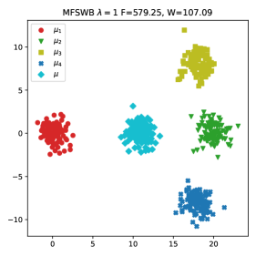
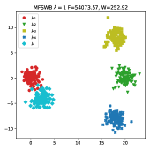
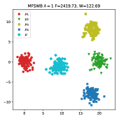
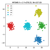
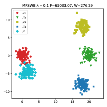
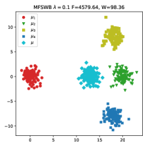
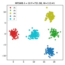
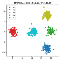
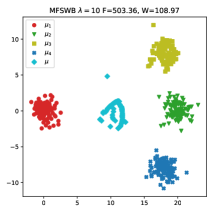
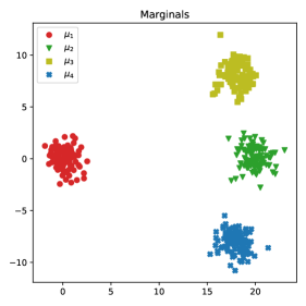
In some applications, we might want to find a barycenter that minimizes the distances to marginals and has equal distances to marginals at the same time e.g., constructing shape template for a group of shapes [3, 46] that can be further used in downstream tasks, exact balance style mixing between images [4], fair generative modeling [7], and so on. We refer to such a barycenter as a marginal fairness barycenter. Both the Wasserstein barycenter and SWB are defined based on a given set of marginal weights (marginal coefficients), and these weights represent the important levels of marginals toward the barycenter. Nevertheless, a uniform (weights) barycenter does not necessarily lead to the desired marginal fairness barycenter as shown in Figure 1. Moreover, obtaining the marginal fairness barycenter is challenging since such a barycenter might not exist and might not be identifiable given non-global-optimal optimization (Karcher mean problem). To the best of our knowledge, there is no prior work that investigates finding a marginal fairness barycenter.
Refer to caption Refer to caption Refer to caption
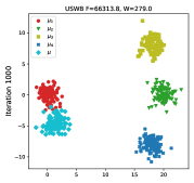
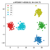
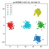
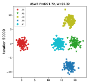
Figure 1: The uniform SWB and the MFSWB of 4 Gaussian distributions.

In this work, we make the first attempt to tackle the marginal fairness barycenter problem i.e., we focus on finding marginal fairness SW barycenter (MFSWB) to utilize the scalability of SW distance.

Contribution: In summary, our main contributions are four-fold:

1. We define the marginal fairness SW barycenter (MFSWB) problem which is a constraint barycenter problem, where the constraint tries to limit the average pair-wise absolute difference between distances from the barycenter to marginals. We derive the dual form of MFSWB, discuss its computation, and address its computational challenges.

2. To address the issue, we propose surrogate definitions of MFSWB which are hyperparameter-free and computationally tractable. Motivated by Fair PCA [40], we propose the first surrogate MFSWB that minimizes the largest SW distance from the barycenter to the marginals. To address the problem of biased gradient estimation of the first surrogate MFSWB, we propose the second surrogate MFSWB which is the expectation of the largest one-dimensional Wasserstein distance from the projected barycenter to the projected marginals. We show that the second surrogate is an upper bound of the first surrogate and can yield an unbiased gradient estimator. We extend further the second surrogates to the third surrogate by applying slicing distribution selection and showing that the third surrogate is an upper bound of the previous two.

3. We discuss the connection between the proposed surrogate MFSWB problems with the sliced multi-marginal Wasserstein (SMW) distance with the maximal ground metric. In particular, solving the proposed MFSWB problems is equivalent to minimizing a lower bound of the SMW. By showing that the SMW with the maximal ground metric is a generalized metric, we convey that it is safe to use the proposed surrogate MFSWB problems.

4. We conduct simulations with Gaussian and experiments on various applications including 3D point-cloud averaging, color harmonization, and sliced Wasserstein autoencoder with class-fairness representation to demonstrate the favorable performance of the proposed surrogate definitions.

Organization. We first discuss some preliminaries on SW distance, SWB and its computation, and sliced multi-marginal Wasserstein distance in Section 2. We then introduce the formal definition and surrogate definitions of marginal fairness SWB in Section 3. After that, we conduct experiments to demonstrate the favorable performance in fairness of the proposed definitions in Section 4. We conclude the paper and provide some future directions in Section 5. Finally, we defer the proofs of key results, the discussion on related works, and additional materials in the Appendices.

2 Preliminaries

Sliced Wasserstein distance. The definition of sliced Wasserstein (SW) distance [4] between two probability measures μ1𝒫p(d)subscript𝜇1subscript𝒫𝑝superscript𝑑\mu_{1}\in\mathcal{P}_{p}(\mathbb{R}^{d}) and μ2𝒫p(d)subscript𝜇2subscript𝒫𝑝superscript𝑑\mu_{2}\in\mathcal{P}_{p}(\mathbb{R}^{d}) is:

SWpp(μ1,μ2)=𝔼θ𝒰(𝕊d1)[Wpp(θμ1,θμ2)],superscriptsubscriptSW𝑝𝑝subscript𝜇1subscript𝜇2subscript𝔼similar-to𝜃𝒰superscript𝕊𝑑1delimited-[]superscriptsubscriptW𝑝𝑝𝜃subscript𝜇1𝜃subscript𝜇2\displaystyle\text{SW}_{p}^{p}(\mu_{1},\mu_{2})=\mathbb{E}_{\theta\sim\mathcal{U}(\mathbb{S}^{d-1})}[\text{W}_{p}^{p}(\theta\sharp\mu_{1},\theta\sharp\mu_{2})], (1)

where the Wasserstein distance has a closed form in one-dimension which is Wpp(θμ1,θμ2)=01|Fθμ11(z)Fθμ21(z)|p𝑑zsuperscriptsubscriptW𝑝𝑝𝜃subscript𝜇1𝜃subscript𝜇2superscriptsubscript01superscriptsuperscriptsubscript𝐹𝜃subscript𝜇11𝑧superscriptsubscript𝐹𝜃subscript𝜇21𝑧𝑝differential-d𝑧\text{W}_{p}^{p}(\theta\sharp\mu_{1},\theta\sharp\mu_{2})=\int_{0}^{1}|F_{\theta\sharp\mu_{1}}^{-1}(z)-F_{\theta\sharp\mu_{2}}^{-1}(z)|^{p}dz where Fθμ1subscript𝐹𝜃subscript𝜇1F_{\theta\sharp\mu_{1}} and Fθμ2subscript𝐹𝜃subscript𝜇2F_{\theta\sharp\mu_{2}} are the cumulative distribution function (CDF) of θμ1𝜃subscript𝜇1\theta\sharp\mu_{1} and θμ2𝜃subscript𝜇2\theta\sharp\mu_{2} respectively.

Sliced Wasserstein Barycenter. The definition of the sliced Wasserstein barycenter (SWB) problem [4] of K2𝐾2K\geq 2 marginals μ1,,μK𝒫p(d)subscript𝜇1subscript𝜇𝐾subscript𝒫𝑝superscript𝑑\mu_{1},\ldots,\mu_{K}\in\mathcal{P}_{p}(\mathbb{R}^{d}) with marginal weights ω1,,ωK>0subscript𝜔1subscript𝜔𝐾0\omega_{1},\ldots,\omega_{K}>0 (i=kKωk=1superscriptsubscript𝑖𝑘𝐾subscript𝜔𝑘1\sum_{i=k}^{K}\omega_{k}=1) is defined as:

minμ(μ;μ1:K,ω1:K);(μ;μ1:K,ω1:K)=k=1KωkSWpp(μ,μk).subscript𝜇𝜇subscript𝜇:1𝐾subscript𝜔:1𝐾𝜇subscript𝜇:1𝐾subscript𝜔:1𝐾superscriptsubscript𝑘1𝐾subscript𝜔𝑘superscriptsubscriptSW𝑝𝑝𝜇subscript𝜇𝑘\displaystyle\min_{\mu}\mathcal{F}(\mu;\mu_{1:K},\omega_{1:K});\quad\mathcal{F}(\mu;\mu_{1:K},\omega_{1:K})=\sum_{k=1}^{K}\omega_{k}\text{SW}_{p}^{p}(\mu,\mu_{k}). (2)

Computation of parametric SWB. Let μϕsubscript𝜇italic-ϕ\mu_{\phi} be parameterized by ϕΦitalic-ϕΦ\phi\in\Phi, SWB can be solved by gradient-based optimization. In that case, the interested quantity is the gradient ϕ(μϕ;μ1:K,ω1:K)=k=1KωkϕSWpp(μϕ,μk)subscriptitalic-ϕsubscript𝜇italic-ϕsubscript𝜇:1𝐾subscript𝜔:1𝐾superscriptsubscript𝑘1𝐾subscript𝜔𝑘subscriptitalic-ϕsuperscriptsubscriptSW𝑝𝑝subscript𝜇italic-ϕsubscript𝜇𝑘\nabla_{\phi}\mathcal{F}(\mu_{\phi};\mu_{1:K},\omega_{1:K})=\sum_{k=1}^{K}\omega_{k}\nabla_{\phi}\text{SW}_{p}^{p}(\mu_{\phi},\mu_{k}). However, the gradient ϕSWpp(μϕ,μk)=ϕ𝔼θ𝒰(𝕊d1)[Wpp(θμϕ,θμk)]=𝔼θ𝒰(𝕊d1)[ϕWpp(θμϕ,θμk)]subscriptitalic-ϕsuperscriptsubscriptSW𝑝𝑝subscript𝜇italic-ϕsubscript𝜇𝑘subscriptitalic-ϕsubscript𝔼similar-to𝜃𝒰superscript𝕊𝑑1delimited-[]superscriptsubscriptW𝑝𝑝𝜃subscript𝜇italic-ϕ𝜃subscript𝜇𝑘subscript𝔼similar-to𝜃𝒰superscript𝕊𝑑1delimited-[]subscriptitalic-ϕsuperscriptsubscriptW𝑝𝑝𝜃subscript𝜇italic-ϕ𝜃subscript𝜇𝑘\nabla_{\phi}\text{SW}_{p}^{p}(\mu_{\phi},\mu_{k})=\nabla_{\phi}\mathbb{E}_{\theta\sim\mathcal{U}(\mathbb{S}^{d-1})}[\text{W}_{p}^{p}(\theta\sharp\mu_{\phi},\theta\sharp\mu_{k})]=\mathbb{E}_{\theta\sim\mathcal{U}(\mathbb{S}^{d-1})}[\nabla_{\phi}\text{W}_{p}^{p}(\theta\sharp\mu_{\phi},\theta\sharp\mu_{k})] for any k=1,,K𝑘1𝐾k=1,\ldots,K is intractable due to the intractability of SW with the expectation with respect to the uniform distribution over the unit-hypersphere. Therefore, Monte Carlo estimation is used. In particular, projecting directions θ1,,θLsubscript𝜃1subscript𝜃𝐿\theta_{1},\ldots,\theta_{L} are sampled i.i.d from 𝒰(𝕊d1)𝒰superscript𝕊𝑑1\mathcal{U}(\mathbb{S}^{d-1}), and the stochastic gradient estimator is formed:

ϕSWpp(μϕ,μk)1Ll=1LϕWpp(θlμϕ,θlμk).subscriptitalic-ϕsuperscriptsubscriptSW𝑝𝑝subscript𝜇italic-ϕsubscript𝜇𝑘1𝐿superscriptsubscript𝑙1𝐿subscriptitalic-ϕsuperscriptsubscriptW𝑝𝑝subscript𝜃𝑙subscript𝜇italic-ϕsubscript𝜃𝑙subscript𝜇𝑘\displaystyle\nabla_{\phi}\text{SW}_{p}^{p}(\mu_{\phi},\mu_{k})\approx\frac{1}{L}\sum_{l=1}^{L}\nabla_{\phi}\text{W}_{p}^{p}(\theta_{l}\sharp\mu_{\phi},\theta_{l}\sharp\mu_{k}). (3)

With the stochastic gradient, the SWB can be solved by using a stochastic gradient descent algorithm. We refer the reader to Algorithm 1 in Appendix B for more detail. Specifically, we now discuss the discrete SWB i.e., marginals and the barycenter are discrete measures.

Free supports barycenter. In this setting, we have μϕ=1ni=1nδxisubscript𝜇italic-ϕ1𝑛superscriptsubscript𝑖1𝑛subscript𝛿subscript𝑥𝑖\mu_{\phi}=\frac{1}{n}\sum_{i=1}^{n}\delta_{x_{i}}, μk=1ni=1nδyisubscript𝜇𝑘1𝑛superscriptsubscript𝑖1𝑛subscript𝛿subscript𝑦𝑖\mu_{k}=\frac{1}{n}\sum_{i=1}^{n}\delta_{y_{i}}, and ϕ=(x1,,xn)italic-ϕsubscript𝑥1subscript𝑥𝑛\phi=(x_{1},\ldots,x_{n}), we can compute the (sub-)gradient with the time complexity 𝒪(nlogn)𝒪𝑛𝑛\mathcal{O}(n\log n):

xiWpp(θμϕ,θμk)=p|θxiθyσ(i)|p1sign(θxiθyσ(i))θ,subscriptsubscript𝑥𝑖superscriptsubscriptW𝑝𝑝𝜃subscript𝜇italic-ϕ𝜃subscript𝜇𝑘𝑝superscriptsuperscript𝜃topsubscript𝑥𝑖superscript𝜃topsubscript𝑦𝜎𝑖𝑝1signsuperscript𝜃topsubscript𝑥𝑖superscript𝜃topsubscript𝑦𝜎𝑖𝜃\displaystyle\nabla_{x_{i}}\text{W}_{p}^{p}(\theta\sharp\mu_{\phi},\theta\sharp\mu_{k})=p|\theta^{\top}x_{i}-\theta^{\top}y_{\sigma(i)}|^{p-1}\text{sign}(\theta^{\top}x_{i}-\theta^{\top}y_{\sigma(i)})\theta, (4)

where σ=σ1σ21𝜎subscript𝜎1superscriptsubscript𝜎21\sigma=\sigma_{1}\circ\sigma_{2}^{-1} with σ1subscript𝜎1\sigma_{1} and σ2subscript𝜎2\sigma_{2} are any sorted permutation of {x1,,xn}subscript𝑥1subscript𝑥𝑛\{x_{1},\ldots,x_{n}\} and {y1,,yn}subscript𝑦1subscript𝑦𝑛\{y_{1},\ldots,y_{n}\}.

Fixed supports barycenter. In this setting, we have μϕ=i=1nϕiδxisubscript𝜇italic-ϕsuperscriptsubscript𝑖1𝑛subscriptitalic-ϕ𝑖subscript𝛿subscript𝑥𝑖\mu_{\phi}=\sum_{i=1}^{n}\phi_{i}\delta_{x_{i}}, μk=i=1nβiδxisubscript𝜇𝑘superscriptsubscript𝑖1𝑛subscript𝛽𝑖subscript𝛿subscript𝑥𝑖\mu_{k}=\sum_{i=1}^{n}\beta_{i}\delta_{x_{i}}, i=1nϕi=i=1nβisuperscriptsubscript𝑖1𝑛subscriptitalic-ϕ𝑖superscriptsubscript𝑖1𝑛subscript𝛽𝑖\sum_{i=1}^{n}\phi_{i}=\sum_{i=1}^{n}\beta_{i} and ϕ=(ϕ1,,ϕn)italic-ϕsubscriptitalic-ϕ1subscriptitalic-ϕ𝑛\phi=(\phi_{1},\ldots,\phi_{n}). We can compute the gradient as follows:

ϕWpp(θμϕ,θμk)=𝒇,subscriptitalic-ϕsuperscriptsubscriptW𝑝𝑝𝜃subscript𝜇italic-ϕ𝜃subscript𝜇𝑘superscript𝒇\displaystyle\nabla_{\phi}\text{W}_{p}^{p}(\theta\sharp\mu_{\phi},\theta\sharp\mu_{k})=\bm{f}^{\star}, (5)

where 𝒇superscript𝒇\bm{f}^{\star} is the first optimal Kantorovich dual potential of Wpp(θμϕ,θμk)superscriptsubscriptW𝑝𝑝𝜃subscript𝜇italic-ϕ𝜃subscript𝜇𝑘\text{W}_{p}^{p}(\theta\sharp\mu_{\phi},\theta\sharp\mu_{k}) which can be obtained with the time complexity of 𝒪(nlogn)𝒪𝑛𝑛\mathcal{O}(n\log n). We refer the reader to Proposition 1 in [12] for the detail and Algorithm 1 in [41] for the computational algorithm.

When the supports or weights of the barycenter are the output of a parametric function, we can use the chain rule to estimate the gradient of the parameters of the function. For the continuous case, we can approximate the barycenter and marginals by their empirical versions, and then perform the estimation in the discrete case. Since the sample complexity of SW is 𝒪(n1/2)𝒪superscript𝑛12\mathcal{O}(n^{-1/2}) [31, 35, 27, 37], the approximation error will reduce fast with the number of support n𝑛n increases. Another option is to use continuous Wasserstein solvers [15, 23, 9], however, this option is not as simple as the first one.

Sliced Multi-marginal Wasserstein Distance. Given K1𝐾1K\geq 1 marginals μ1,,μK𝒫p(d)subscript𝜇1subscript𝜇𝐾subscript𝒫𝑝superscript𝑑\mu_{1},\ldots,\mu_{K}\in\mathcal{P}_{p}(\mathbb{R}^{d}), sliced Multi-marginal Wasserstein Distance [10] (SMW) is defined as:

SMWpp(μ1:K;c)=𝔼[infπΠ(μ1,,μK)c(θx1,,θxK)p𝑑π(x1,,xK)],𝑆𝑀superscriptsubscript𝑊𝑝𝑝subscript𝜇:1𝐾𝑐𝔼delimited-[]subscriptinfimum𝜋Πsubscript𝜇1subscript𝜇𝐾𝑐superscriptsuperscript𝜃topsubscript𝑥1superscript𝜃topsubscript𝑥𝐾𝑝differential-d𝜋subscript𝑥1subscript𝑥𝐾\displaystyle SMW_{p}^{p}(\mu_{1:K};c)=\mathbb{E}\left[\inf_{\pi\in\Pi(\mu_{1},\ldots,\mu_{K})}\int c(\theta^{\top}x_{1},\ldots,\theta^{\top}x_{K})^{p}d\pi(x_{1},\ldots,x_{K})\right], (6)

where the expectation is under θ𝒰(𝕊d1)similar-to𝜃𝒰superscript𝕊𝑑1\theta\sim\mathcal{U}(\mathbb{S}^{d-1}). When using the barycentric cost i.e., c(θx1,,θxK)p=k=1Kβk|θxkk=1Kβkθxk|p𝑐superscriptsuperscript𝜃topsubscript𝑥1superscript𝜃topsubscript𝑥𝐾𝑝superscriptsubscript𝑘1𝐾subscript𝛽𝑘superscriptsuperscript𝜃topsubscript𝑥𝑘superscriptsubscriptsuperscript𝑘1𝐾subscript𝛽superscript𝑘superscript𝜃topsubscript𝑥superscript𝑘𝑝c(\theta^{\top}x_{1},\ldots,\theta^{\top}x_{K})^{p}=\sum_{k=1}^{K}\beta_{k}\left|\theta^{\top}x_{k}-\sum_{k^{\prime}=1}^{K}\beta_{k^{\prime}}\theta^{\top}x_{k^{\prime}}\right|^{p} for βk>0ksubscript𝛽𝑘0for-all𝑘\beta_{k}>0\forall k and kβk=1subscript𝑘subscript𝛽𝑘1\sum_{k}\beta_{k}=1. Minimizing SMWpp(μ1:K,μ;c)𝑆𝑀superscriptsubscript𝑊𝑝𝑝subscript𝜇:1𝐾𝜇𝑐SMW_{p}^{p}(\mu_{1:K},\mu;c) with respect to μ𝜇\mu is equivalent to a barycenter problem. We refer the reader to Proposition 7 in [10] for more detail.

3 Marginal Fairness Sliced Wasserstein Barycenter

We first formally define the marginal fairness Sliced Wasserstein barycenter in Section 3.1. We then propose surrogate problems in Section 3.2. Finally, we discuss the connection of the proposed surrogate problems to sliced multi-marginal Wasserstein in Section 3.3.

3.1 Formal Definition

Now, we define the Marginal Fairness Sliced Wasserstein barycenter (MFSWB) problem by adding marginal fairness constraints to the SWB problem.

Definition 1.

Given K2𝐾2K\geq 2 marginals μ1,,μK𝒫p(d)subscript𝜇1subscript𝜇𝐾subscript𝒫𝑝superscript𝑑\mu_{1},\ldots,\mu_{K}\in\mathcal{P}_{p}(\mathbb{R}^{d}), admissible ϵ0italic-ϵ0\epsilon\geq 0 for i=1,,K𝑖1𝐾i=1,\ldots,K and j=i+1,,K𝑗𝑖1𝐾j=i+1,\ldots,K, the Marginal Fairness Sliced Wasserstein barycenter (MFSWB) is defined as:

minμ1Kk=1KSWpp(μ,μk) s.t. 2(K1)Ki=1Kj=i+1K|SWpp(μ,μi)SWpp(μ,μj)|ϵ.subscript𝜇1𝐾superscriptsubscript𝑘1𝐾superscriptsubscriptSW𝑝𝑝𝜇subscript𝜇𝑘 s.t. 2𝐾1𝐾superscriptsubscript𝑖1𝐾superscriptsubscript𝑗𝑖1𝐾superscriptsubscriptSW𝑝𝑝𝜇subscript𝜇𝑖superscriptsubscriptSW𝑝𝑝𝜇subscript𝜇𝑗italic-ϵ\displaystyle\min_{\mu}\frac{1}{K}\sum_{k=1}^{K}\text{SW}_{p}^{p}(\mu,\mu_{k})\text{ s.t. }\frac{2}{(K-1)K}\sum_{i=1}^{K}\sum_{j=i+1}^{K}|\text{SW}_{p}^{p}(\mu,\mu_{i})-\text{SW}_{p}^{p}(\mu,\mu_{j})|\leq\epsilon. (7)
Remark.

We want ϵitalic-ϵ\epsilon in Definition 1 to be close to 00 i.e., μ1,,μKsubscript𝜇1subscript𝜇𝐾\mu_{1},\ldots,\mu_{K} are on the SWp𝑆subscript𝑊𝑝SW_{p}-sphere with the center μ𝜇\mu. However, for a too-small value of ϵitalic-ϵ\epsilon, there might not exist a solution μ𝜇\mu.

Duality objective. For admissible ϵ>0italic-ϵ0\epsilon>0, there exist a Lagrange multiplier λ𝜆\lambda such that we have the dual form

(μ,λ)=1Kk=1KSWpp(μ,μk)+2λ(K1)Ki=1Kj=i+1K|SWpp(μ,μi)SWpp(μ,μj)|λϵ.𝜇𝜆1𝐾superscriptsubscript𝑘1𝐾superscriptsubscriptSW𝑝𝑝𝜇subscript𝜇𝑘2𝜆𝐾1𝐾superscriptsubscript𝑖1𝐾superscriptsubscript𝑗𝑖1𝐾superscriptsubscriptSW𝑝𝑝𝜇subscript𝜇𝑖superscriptsubscriptSW𝑝𝑝𝜇subscript𝜇𝑗𝜆italic-ϵ\displaystyle\mathcal{L}(\mu,\lambda)=\frac{1}{K}\sum_{k=1}^{K}\text{SW}_{p}^{p}(\mu,\mu_{k})+\frac{2\lambda}{(K-1)K}\sum_{i=1}^{K}\sum_{j=i+1}^{K}|\text{SW}_{p}^{p}(\mu,\mu_{i})-\text{SW}_{p}^{p}(\mu,\mu_{j})|-\lambda\epsilon. (8)

Computational challenges. Firstly, MFSWB in Definition 1 requires admissible ϵ>0italic-ϵ0\epsilon>0 to guarantee the existence of the barycenter μ𝜇\mu. In practice, it is unknown if a value of ϵitalic-ϵ\epsilon satisfies such a property. Secondly, given a ϵitalic-ϵ\epsilon, it is not trivial to obtain the optimal Lagrange multiplier λsuperscript𝜆\lambda^{\star} in Equation equation 8 to minimize the duality gap which can be non-zero (weak-duality). Thirdly, using directly the dual objective Equation equation 8 requires hyperparameter tunning for λ𝜆\lambda and might not provide a good landscape for optimization. Moreover, we cannot obtain an unbiased gradient estimate of ϕitalic-ϕ\phi in the case of the parametric barycenter μϕsubscript𝜇italic-ϕ\mu_{\phi}. In greater detail, the Monte Carlo estimation for the absolute distance between two SW distances is biased. Finally, Equation equation 8 has a quadratic time complexity and space complexity in terms of the number of marginals i.e., 𝒪(K2)𝒪superscript𝐾2\mathcal{O}(K^{2}).

3.2 Surrogate Definitions

Since it is not convenient to use the formal MFSWB in applications, we propose two surrogate definitions of MFSWB that are free of hyperparameters and computationally friendly.

First Surrogate Definition. Motivated by Fair PCA [40], we propose a practical surrogate MFSWB problem that is hyperparameter-free.

Definition 2.

Given K2𝐾2K\geq 2 marginals μ1,,μK𝒫p(d)subscript𝜇1subscript𝜇𝐾subscript𝒫𝑝superscript𝑑\mu_{1},\ldots,\mu_{K}\in\mathcal{P}_{p}(\mathbb{R}^{d}), the surrogate marginal fairness sliced Wasserstein barycenter (s-MFSWB) problem is defined as:

minμ𝒮(μ;μ1:K);𝒮(μ;μ1:K)=maxk{1,,K}SWpp(μ,μk).subscript𝜇𝒮𝜇subscript𝜇:1𝐾𝒮𝜇subscript𝜇:1𝐾subscript𝑘1𝐾𝑆superscriptsubscript𝑊𝑝𝑝𝜇subscript𝜇𝑘\displaystyle\min_{\mu}\mathcal{SF}(\mu;\mu_{1:K});\quad\mathcal{SF}(\mu;\mu_{1:K})=\max_{k\in\{1,\ldots,K\}}SW_{p}^{p}(\mu,\mu_{k}). (9)

The s-MFSWB problem tries to minimize the maximal distance from the barycenter to the marginals. Therefore, it can minimize indirectly the overall distances between the barycenter to the marginals and implicitly make the distances to marginals approximately the same.

Gradient estimator. Let μϕsubscript𝜇italic-ϕ\mu_{\phi} be paramterized by ϕΦitalic-ϕΦ\phi\in\Phi, and (ϕ,k)=SWpp(μϕ,μk)italic-ϕ𝑘𝑆superscriptsubscript𝑊𝑝𝑝subscript𝜇italic-ϕsubscript𝜇𝑘\mathcal{F}(\phi,k)=SW_{p}^{p}(\mu_{\phi},\mu_{k}), we would like to compute ϕmaxk{1,,K}(ϕ,k)subscriptitalic-ϕsubscript𝑘1𝐾italic-ϕ𝑘\nabla_{\phi}\max_{k\in\{1,\ldots,K\}}\mathcal{F}(\phi,k). By Danskin’s envelope theorem [13], we have ϕmaxk{1,,K}(ϕ,k)=ϕ(ϕ,k)=ϕSWpp(μϕ,μk)subscriptitalic-ϕsubscript𝑘1𝐾italic-ϕ𝑘subscriptitalic-ϕitalic-ϕsuperscript𝑘subscriptitalic-ϕsuperscriptsubscriptSW𝑝𝑝subscript𝜇italic-ϕsubscript𝜇superscript𝑘\nabla_{\phi}\max_{k\in\{1,\ldots,K\}}\mathcal{F}(\phi,k)=\nabla_{\phi}\mathcal{F}(\phi,k^{\star})=\nabla_{\phi}\text{SW}_{p}^{p}(\mu_{\phi},\mu_{k^{\star}}) for k=argmaxk{1,,K}(ϕ,k)superscript𝑘subscriptargmax𝑘1𝐾italic-ϕ𝑘k^{\star}=\operatorname*{arg\,max}_{k\in\{1,\ldots,K\}}\mathcal{F}(\phi,k). Nevertheless, ksuperscript𝑘k^{\star} is intractable due to the intractablity of SWpp(μϕ,μk)𝑆superscriptsubscript𝑊𝑝𝑝subscript𝜇italic-ϕsubscript𝜇𝑘SW_{p}^{p}(\mu_{\phi},\mu_{k}) for k=1,,K𝑘1𝐾k=1,\ldots,K. Hence, we can form the estimation k^=argmaxk{1,,K}SW^pp(μϕ,μk;L)superscript^𝑘subscriptargmax𝑘1𝐾superscriptsubscript^𝑆𝑊𝑝𝑝subscript𝜇italic-ϕsubscript𝜇𝑘𝐿\hat{k}^{\star}=\operatorname*{arg\,max}_{k\in\{1,\ldots,K\}}\widehat{SW}_{p}^{p}(\mu_{\phi},\mu_{k};L) where SW^pp(μϕ,μk;L)=1Ll=1LWpp(θlμϕ,θlμk)superscriptsubscript^𝑆𝑊𝑝𝑝subscript𝜇italic-ϕsubscript𝜇𝑘𝐿1𝐿superscriptsubscript𝑙1𝐿superscriptsubscriptW𝑝𝑝subscript𝜃𝑙subscript𝜇italic-ϕsubscript𝜃𝑙subscript𝜇𝑘\widehat{SW}_{p}^{p}(\mu_{\phi},\mu_{k};L)=\frac{1}{L}\sum_{l=1}^{L}\text{W}_{p}^{p}(\theta_{l}\sharp\mu_{\phi},\theta_{l}\sharp\mu_{k}) with θ1,,θLi.i.d𝒰(𝕊d1)subscript𝜃1subscript𝜃𝐿formulae-sequence𝑖𝑖𝑑similar-to𝒰superscript𝕊𝑑1\theta_{1},\ldots,\theta_{L}\overset{i.i.d}{\sim}\mathcal{U}(\mathbb{S}^{d-1}). Then, we can estimate ϕSWpp(μϕ,μk^)subscriptitalic-ϕsuperscriptsubscriptSW𝑝𝑝subscript𝜇italic-ϕsubscript𝜇superscript^𝑘\nabla_{\phi}\text{SW}_{p}^{p}(\mu_{\phi},\mu_{\hat{k}^{\star}}) as in Equation 3. We refer the reader to Algorithm 2 in Appendix B for the gradient estimation and optimization procedure. The downside of this estimator is that it is biased.

Second Surrogate Definition. To address the biased gradient issue of the first surrogate problem, we propose the second surrogate MFSWB problem.

Definition 3.

Given K2𝐾2K\geq 2 marginals μ1,,μK𝒫p(d)subscript𝜇1subscript𝜇𝐾subscript𝒫𝑝superscript𝑑\mu_{1},\ldots,\mu_{K}\in\mathcal{P}_{p}(\mathbb{R}^{d}), the unbiased surrogate marginal fairness sliced Wasserstein barycenter (us-MFSWB) problem is defined as:

minμ𝒰𝒮(μ;μ1:K);𝒰𝒮(μ;μ1:K)=𝔼θ𝒰(𝕊d1)[maxk{1,,K}Wpp(θμ,θμk)].subscript𝜇𝒰𝒮𝜇subscript𝜇:1𝐾𝒰𝒮𝜇subscript𝜇:1𝐾subscript𝔼similar-to𝜃𝒰superscript𝕊𝑑1delimited-[]subscript𝑘1𝐾superscriptsubscript𝑊𝑝𝑝𝜃𝜇𝜃subscript𝜇𝑘\displaystyle\min_{\mu}\mathcal{USF}(\mu;\mu_{1:K});\quad\mathcal{USF}(\mu;\mu_{1:K})=\mathbb{E}_{\theta\sim\mathcal{U}(\mathbb{S}^{d-1})}\left[\max_{k\in\{1,\ldots,K\}}W_{p}^{p}(\theta\sharp\mu,\theta\sharp\mu_{k})\right]. (10)

In contrast to s-MFSWB which minimizes the maximal SW distance among marginals, us-MFSWB minimizes the expected value of the maximal one-dimensional Wasserstein distance among marginals. By considering fairness on one-dimensional projections, us-MFSWB can yield an unbiased gradient estimate which is the reason why it is named as unbiased s-MFSWB.

Gradient estimator. Let μϕsubscript𝜇italic-ϕ\mu_{\phi} be paramterized by ϕΦitalic-ϕΦ\phi\in\Phi, and (θ,ϕ,k)=Wpp(θμϕ,θμk)𝜃italic-ϕ𝑘superscriptsubscript𝑊𝑝𝑝𝜃subscript𝜇italic-ϕ𝜃subscript𝜇𝑘\mathcal{F}(\theta,\phi,k)=W_{p}^{p}(\theta\sharp\mu_{\phi},\theta\sharp\mu_{k}), we would like to compute ϕ𝔼θ𝕊d1[maxk{1,,K}(θ,ϕ,k)]subscriptitalic-ϕsubscript𝔼similar-to𝜃superscript𝕊𝑑1delimited-[]subscript𝑘1𝐾𝜃italic-ϕ𝑘\nabla_{\phi}\mathbb{E}_{\theta\sim\mathbb{S}^{d-1}}[\max_{k\in\{1,\ldots,K\}}\mathcal{F}(\theta,\phi,k)] which is equivalent to 𝔼θ𝕊d1[ϕmaxk{1,,K}(θ,ϕ,k)]subscript𝔼similar-to𝜃superscript𝕊𝑑1delimited-[]subscriptitalic-ϕsubscript𝑘1𝐾𝜃italic-ϕ𝑘\mathbb{E}_{\theta\sim\mathbb{S}^{d-1}}[\nabla_{\phi}\max_{k\in\{1,\ldots,K\}}\mathcal{F}(\theta,\phi,k)] due to the Leibniz’s rule. By Danskin’s envelope theorem, we have ϕmaxk{1,,K}(θ,ϕ,k)=ϕ(θ,ϕ,k)=ϕWpp(θμϕ,θμk)subscriptitalic-ϕsubscript𝑘1𝐾𝜃italic-ϕ𝑘subscriptitalic-ϕ𝜃italic-ϕsuperscript𝑘subscriptitalic-ϕsuperscriptsubscriptW𝑝𝑝𝜃subscript𝜇italic-ϕ𝜃subscript𝜇superscript𝑘\nabla_{\phi}\max_{k\in\{1,\ldots,K\}}\mathcal{F}(\theta,\phi,k)=\nabla_{\phi}\mathcal{F}(\theta,\phi,k^{\star})=\nabla_{\phi}\text{W}_{p}^{p}(\theta\sharp\mu_{\phi},\theta\sharp\mu_{k^{\star}}) for kθ=argmaxk{1,,K}(θ,ϕ,k)subscriptsuperscript𝑘𝜃subscriptargmax𝑘1𝐾𝜃italic-ϕ𝑘k^{\star}_{\theta}=\operatorname*{arg\,max}_{k\in\{1,\ldots,K\}}\mathcal{F}(\theta,\phi,k) where we can estimate ϕWpp(θμϕ,θμkθ)subscriptitalic-ϕsuperscriptsubscriptW𝑝𝑝𝜃subscript𝜇italic-ϕ𝜃subscript𝜇subscriptsuperscript𝑘𝜃\nabla_{\phi}\text{W}_{p}^{p}(\theta\sharp\mu_{\phi},\theta\sharp\mu_{k^{\star}_{\theta}}) can be computed as in Equation 45. Overall, with θ1,,θLi.i.d𝒰(𝕊d1)subscript𝜃1subscript𝜃𝐿formulae-sequence𝑖𝑖𝑑similar-to𝒰superscript𝕊𝑑1\theta_{1},\ldots,\theta_{L}\overset{i.i.d}{\sim}\mathcal{U}(\mathbb{S}^{d-1}), we can form the final estimation 1Ll=1LϕWpp(θlμϕ,θlμkθl)1𝐿superscriptsubscript𝑙1𝐿subscriptitalic-ϕsuperscriptsubscriptW𝑝𝑝subscript𝜃𝑙subscript𝜇italic-ϕsubscript𝜃𝑙subscript𝜇subscriptsuperscript𝑘subscript𝜃𝑙\frac{1}{L}\sum_{l=1}^{L}\nabla_{\phi}\text{W}_{p}^{p}(\theta_{l}\sharp\mu_{\phi},\theta_{l}\sharp\mu_{k^{\star}_{\theta_{l}}}) which is an unbiased estimate. We refer the reader to Algorithm 3 in Appendix B for the gradient estimation and optimization procedure.

Proposition 1.

Given K2𝐾2K\geq 2 marginals μ1:K𝒫p(d)subscript𝜇:1𝐾subscript𝒫𝑝superscript𝑑\mu_{1:K}\in\mathcal{P}_{p}(\mathbb{R}^{d}), we have 𝒮(μ;μ1:K)𝒰𝒮(μ;μ1:K)𝒮𝜇subscript𝜇:1𝐾𝒰𝒮𝜇subscript𝜇:1𝐾\mathcal{SF}(\mu;\mu_{1:K})\leq\mathcal{USF}(\mu;\mu_{1:K}).

Proof of Proposition 1 is given in Appendix A.1. From the proposition, we see that minimizing the objective of us-MFSWB also reduces the objective of s-MFSWB implicitly.

Proposition 2.

Given K2𝐾2K\geq 2 marginals μ1,,μK𝒫p(d)subscript𝜇1subscript𝜇𝐾subscript𝒫𝑝superscript𝑑\mu_{1},\ldots,\mu_{K}\in\mathcal{P}_{p}(\mathbb{R}^{d}), θ1,,θLi.i.d𝒰(𝕊d1)subscript𝜃1subscript𝜃𝐿formulae-sequence𝑖𝑖𝑑similar-to𝒰superscript𝕊𝑑1\theta_{1},\ldots,\theta_{L}\overset{i.i.d}{\sim}\mathcal{U}(\mathbb{S}^{d-1}), we have:

𝔼|ϕ1Ll=1LWpp(θlμϕ,θlμkθ)ϕ𝒰𝒮(μϕ;μ1:K)|1LVar[ϕWpp(θμϕ,θμkθ)]12,𝔼subscriptitalic-ϕ1𝐿superscriptsubscript𝑙1𝐿superscriptsubscriptW𝑝𝑝subscript𝜃𝑙subscript𝜇italic-ϕsubscript𝜃𝑙subscript𝜇subscriptsuperscript𝑘𝜃subscriptitalic-ϕ𝒰𝒮subscript𝜇italic-ϕsubscript𝜇:1𝐾1𝐿Varsuperscriptdelimited-[]subscriptitalic-ϕsuperscriptsubscriptW𝑝𝑝𝜃subscript𝜇italic-ϕ𝜃subscript𝜇subscriptsuperscript𝑘𝜃12\displaystyle\mathbb{E}\left|\nabla_{\phi}\frac{1}{L}\sum_{l=1}^{L}\text{W}_{p}^{p}(\theta_{l}\sharp\mu_{\phi},\theta_{l}\sharp\mu_{k^{\star}_{\theta}})-\nabla_{\phi}\mathcal{USF}(\mu_{\phi};\mu_{1:K})\right|\leq\frac{1}{\sqrt{L}}\text{Var}\left[\nabla_{\phi}\text{W}_{p}^{p}(\theta\sharp\mu_{\phi},\theta\sharp\mu_{k^{\star}_{\theta}})\right]^{\frac{1}{2}}, (11)

where kθ=argmaxk{1,,K}Wpp(θμϕ,θμk)subscriptsuperscript𝑘𝜃subscriptargmax𝑘1𝐾superscriptsubscript𝑊𝑝𝑝𝜃subscript𝜇italic-ϕ𝜃subscript𝜇𝑘k^{\star}_{\theta}=\operatorname*{arg\,max}_{k\in\{1,\ldots,K\}}W_{p}^{p}(\theta\sharp\mu_{\phi},\theta\sharp\mu_{k}); and the expectation and variance are under the random projecting direction θ𝒰(𝕊d1)similar-to𝜃𝒰superscript𝕊𝑑1\theta\sim\mathcal{U}(\mathbb{S}^{d-1})

Proof of Proposition 2 is given in Appendix A.2. From the proposition, we know that the approximation error of the gradient estimator of us-MFSWB reduces at the order of 𝒪(L1/2)𝒪superscript𝐿12\mathcal{O}(L^{-1/2}). Therefore, increasing L𝐿L leads to a better gradient approximation. The approximation could be further improved via Quasi-Monte Carlo methods [32].

Third Surrogate Definition. The us-MFSWB in Definition 3 utilizes the uniform distribution as the slicing distribution, which is empirically shown to be non-optimal in statistical estimation [35]. Following the slicing distribution selection approach in [33], we propose the third surrogate with a new slicing distribution that focuses on unfair projecting directions.

Marginal fairness energy-based slicing distribution. Since we want to encourage marginal fairness, it is natural to construct the slicing distribution based on fairness energy.

Definition 4.

Given K2𝐾2K\geq 2 marginals μ1,,μK𝒫p(d)subscript𝜇1subscript𝜇𝐾subscript𝒫𝑝superscript𝑑\mu_{1},\ldots,\mu_{K}\in\mathcal{P}_{p}(\mathbb{R}^{d}), the marginal fairness energy-based slicing distribution σ(θ;μ,μ1:K)𝒫(𝕊d1)𝜎𝜃𝜇subscript𝜇:1𝐾𝒫superscript𝕊𝑑1\sigma(\theta;\mu,\mu_{1:K})\in\mathcal{P}(\mathbb{S}^{d-1}) is defined with the density function as follow:

fσ(θ;μ,μ1:K)exp(maxk{1,,K}Wpp(θμ,θμk)),proportional-tosubscript𝑓𝜎𝜃𝜇subscript𝜇:1𝐾subscript𝑘1𝐾superscriptsubscript𝑊𝑝𝑝𝜃𝜇𝜃subscript𝜇𝑘\displaystyle f_{\sigma}(\theta;\mu,\mu_{1:K})\propto\exp\left(\max_{k\in\{1,\ldots,K\}}W_{p}^{p}(\theta\sharp\mu,\theta\sharp\mu_{k})\right), (12)

We see that the marginal fairness energy-based slicing distribution in Definition 4 put more mass to a projecting direction θ𝜃\theta that has the larger maximal one-dimensional Wasserstein distance to marginals. Therefore, it will penalize more marginally unfair projecting directions.

Energy-based surrogate MFSWB. From the new proposed slicing distribution, we can define a new surrogate MFSWB problem, named energy-based surrogate MFSWB.

Definition 5.

Given K2𝐾2K\geq 2 marginals μ1,,μK𝒫p(d)subscript𝜇1subscript𝜇𝐾subscript𝒫𝑝superscript𝑑\mu_{1},\ldots,\mu_{K}\in\mathcal{P}_{p}(\mathbb{R}^{d}), the energy-based surrogate marginal fairness sliced Wasserstein barycenter (us-MFSWB) problem is defined as:

minμ𝒮(μ;μ1:K);𝒮(μ;μ1:K)=𝔼θσ(θ;μ,μ1:K)[maxk{1,,K}Wpp(θμ,θμk)].subscript𝜇𝒮𝜇subscript𝜇:1𝐾𝒮𝜇subscript𝜇:1𝐾subscript𝔼similar-to𝜃𝜎𝜃𝜇subscript𝜇:1𝐾delimited-[]subscript𝑘1𝐾superscriptsubscript𝑊𝑝𝑝𝜃𝜇𝜃subscript𝜇𝑘\displaystyle\min_{\mu}\mathcal{ESF}(\mu;\mu_{1:K});\quad\mathcal{ESF}(\mu;\mu_{1:K})=\mathbb{E}_{\theta\sim\sigma(\theta;\mu,\mu_{1:K})}\left[\max_{k\in\{1,\ldots,K\}}W_{p}^{p}(\theta\sharp\mu,\theta\sharp\mu_{k})\right]. (13)

Similar to the us-MFSWB, es-MFSWB utilizes the implicit one-dimensional marginal fairness. Nevertheless, es-MFSWB utilizes the marginal fairness energy-based slicing distribution to reweight the importance of each projecting direction instead of considering them equally.

Proposition 3.

Given K2𝐾2K\geq 2 marginals μ1:K𝒫p(d)subscript𝜇:1𝐾subscript𝒫𝑝superscript𝑑\mu_{1:K}\in\mathcal{P}_{p}(\mathbb{R}^{d}), we have 𝒰𝒮(μ;μ1:K)𝒮(μ;μ1:K)𝒰𝒮𝜇subscript𝜇:1𝐾𝒮𝜇subscript𝜇:1𝐾\mathcal{USF}(\mu;\mu_{1:K})\leq\mathcal{ESF}(\mu;\mu_{1:K}).

Proof of Proposition 3 is given in Appendix A.3. From the proposition, we see that minimizing the objective of es-MFSWB reduces the objective of us-MFSWB implicitly which also decreases the objective of s-MFSWB (Proposition 1).

Gradient estimator. Let μϕsubscript𝜇italic-ϕ\mu_{\phi} be parameterized by ϕΦitalic-ϕΦ\phi\in\Phi, we want to estimate ϕ𝒮(μϕ;μ1:K)subscriptitalic-ϕ𝒮subscript𝜇italic-ϕsubscript𝜇:1𝐾\nabla_{\phi}\mathcal{ESF}(\mu_{\phi};\mu_{1:K}). Since the slicing distribution is unnormalized, we use importance sampling to form an estimation. With θ1,,θLi.i.d𝒰(𝕊d1)subscript𝜃1subscript𝜃𝐿formulae-sequence𝑖𝑖𝑑similar-to𝒰superscript𝕊𝑑1\theta_{1},\ldots,\theta_{L}\overset{i.i.d}{\sim}\mathcal{U}(\mathbb{S}^{d-1}), we can form the importance sampling stochastic gradient estimation:

^ϕ𝒮(μϕ;μ1:K,L)=1Ll=1L[ϕ(Wpp(θlμ,θlμkθl)exp(Wpp(θlμ,θlμkθl))1Li=1L[exp(Wpp(θiμ,θiμkθi))])],subscript^italic-ϕ𝒮subscript𝜇italic-ϕsubscript𝜇:1𝐾𝐿1𝐿superscriptsubscript𝑙1𝐿delimited-[]subscriptitalic-ϕsuperscriptsubscript𝑊𝑝𝑝subscript𝜃𝑙𝜇subscript𝜃𝑙subscript𝜇subscriptsuperscript𝑘subscript𝜃𝑙superscriptsubscript𝑊𝑝𝑝subscript𝜃𝑙𝜇subscript𝜃𝑙subscript𝜇subscriptsuperscript𝑘subscript𝜃𝑙1𝐿superscriptsubscript𝑖1𝐿delimited-[]superscriptsubscript𝑊𝑝𝑝subscript𝜃𝑖𝜇subscript𝜃𝑖subscript𝜇subscriptsuperscript𝑘subscript𝜃𝑖\displaystyle\hat{\nabla}_{\phi}\mathcal{ESF}(\mu_{\phi};\mu_{1:K},L)=\frac{1}{L}\sum_{l=1}^{L}\left[\nabla_{\phi}\left(W_{p}^{p}(\theta_{l}\sharp\mu,\theta_{l}\sharp\mu_{k^{\star}_{\theta_{l}}})\frac{\exp\left(W_{p}^{p}(\theta_{l}\sharp\mu,\theta_{l}\sharp\mu_{k^{\star}_{\theta_{l}}})\right)}{\frac{1}{L}\sum_{i=1}^{L}\left[\exp\left(W_{p}^{p}(\theta_{i}\sharp\mu,\theta_{i}\sharp\mu_{k^{\star}_{\theta_{i}}})\right)\right]}\right)\right],

which can be further derived by using the chain rule and previously discussed techniques. It is worth noting that the above estimation is only asymptotically unbiased. We refer the reader to Algorithm 4 in Appendix B for the gradient estimation and optimization procedure.

Computational complexities of proposed surrogates. For the number of marginals K𝐾K, the three proposed surrogates have a linear time complexity and space complexity i.e., 𝒪(K)𝒪𝐾\mathcal{O}(K) which is the same as the conventional SWB and is better than 𝒪(K2)𝒪superscript𝐾2\mathcal{O}(K^{2}) of the formal MFSWB. For the number of projections L𝐿L, the number of supports n𝑛n, and the number of dimensions d𝑑d, the proposed surrogates have the time complexity of 𝒪(Ln(logn+d))𝒪𝐿𝑛𝑛𝑑\mathcal{O}(Ln(\log n+d)) and the space complexity of 𝒪(L(n+d))𝒪𝐿𝑛𝑑\mathcal{O}(L(n+d)) which are similar to the formal MFSWB and SWB.

3.3 Sliced multi-marginal Wasserstein distance with the maximal ground metric

To shed some light on the proposed substrates, we connect them to a special variant of Sliced multi-marginal Wasserstein (SMW) (see Equation 6) i.e., SMW with the maximal ground metric c(θx1,,θxK)=maxi{1,,K},j{1,,K}|θxiθxj|𝑐superscript𝜃topsubscript𝑥1superscript𝜃topsubscript𝑥𝐾subscriptformulae-sequence𝑖1𝐾𝑗1𝐾superscript𝜃topsubscript𝑥𝑖superscript𝜃topsubscript𝑥𝑗c(\theta^{\top}x_{1},\ldots,\theta^{\top}x_{K})=\max_{i\in\{1,\ldots,K\},j\in\{1,\ldots,K\}}|\theta^{\top}x_{i}-\theta^{\top}x_{j}|. We first show that SMW with the maximal ground metric is a generalized metric on the space of probability measures.

Proposition 4.

Sliced multi-marginal Wasserstein distance with the maximal ground metric is a generalized metric i.e., it satisfies non-negativity, marginal exchangeability, generalized triangle inequality, and identity of identity of indiscernibles.

Proof of Proposition 4 is given in Appendix A.4. It is worth noting that SMW with the maximal ground metric has never been defined before. Since our work focuses on the MFSWB problem, we will leave the careful investigation of this variant of SMW to future work.

Proposition 5.

Given K2𝐾2K\geq 2 marginals μ1,,μK𝒫p(d)subscript𝜇1subscript𝜇𝐾subscript𝒫𝑝superscript𝑑\mu_{1},\ldots,\mu_{K}\in\mathcal{P}_{p}(\mathbb{R}^{d}), the maximal ground metric c(θx1,,θxK)=maxi{1,,K},j{1,,K}|θxiθxj|𝑐superscript𝜃topsubscript𝑥1superscript𝜃topsubscript𝑥𝐾subscriptformulae-sequence𝑖1𝐾𝑗1𝐾superscript𝜃topsubscript𝑥𝑖superscript𝜃topsubscript𝑥𝑗c(\theta^{\top}x_{1},\ldots,\theta^{\top}x_{K})=\max_{i\in\{1,\ldots,K\},j\in\{1,\ldots,K\}}|\theta^{\top}x_{i}-\theta^{\top}x_{j}|, we have:

minμ1𝒰𝒮(μ1;μ2:K)minμ1SMWpp(μ1,μ2,,μK;c).subscriptsubscript𝜇1𝒰𝒮subscript𝜇1subscript𝜇:2𝐾subscriptsubscript𝜇1𝑆𝑀superscriptsubscript𝑊𝑝𝑝subscript𝜇1subscript𝜇2subscript𝜇𝐾𝑐\displaystyle\min_{\mu_{1}}\mathcal{USF}(\mu_{1};\mu_{2:K})\leq\min_{\mu_{1}}SMW_{p}^{p}(\mu_{1},\mu_{2},\ldots,\mu_{K};c). (14)

Proof of Proposition 5 is given in Appendix A.5 and the inequality holds when changing μ1subscript𝜇1\mu_{1} to any μisubscript𝜇𝑖\mu_{i} with i=2,,K𝑖2𝐾i=2,\ldots,K. Combining Proposition 1, we have the corollary of minμ1𝒮(μ1;μ2:K)minμ1SMWpp(μ1,μ2,,μK;c)subscriptsubscript𝜇1𝒮subscript𝜇1subscript𝜇:2𝐾subscriptsubscript𝜇1𝑆𝑀superscriptsubscript𝑊𝑝𝑝subscript𝜇1subscript𝜇2subscript𝜇𝐾𝑐\min_{\mu_{1}}\mathcal{SF}(\mu_{1};\mu_{2:K})\leq\min_{\mu_{1}}SMW_{p}^{p}(\mu_{1},\mu_{2},\ldots,\mu_{K};c). From the proposition, we see that minimizing the us-MFSWB is equivalent to minimizing a lower bound of SMW with the maximal ground metric. Therefore, this proposition implies the us-MFSWB could try to minimize the multi-marginal distance. Moreover, this proposition can help to understand the proposed surrogates through the gradient flow of SMW. We can further extend the proposition to show the minimizing es-MFSWB objective is the same as minimizing a lower bound of energy-based SMW with the maximal ground metric, a new special variant of SMW. We refer the reader to Propositon 6 in Appendix B for more detail.
Refer to caption Refer to caption Refer to caption Refer to caption Refer to caption
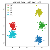
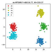
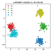
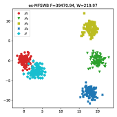
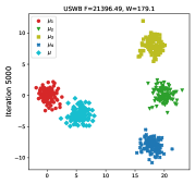
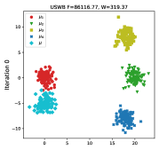
Figure 2: Barycenters from USWB, MFSWB with λ=1𝜆1\lambda=1, s-MFSWB, us-MFSWB, and es-MFSWB along gradient iterations with the corresponding F-metric and W-metric.

4 Experiments

In this section, we compare the barycenter found by our proposed surrogate problems i.e., s-MFSWB, us-MFSWB, and es-MFSWB with the barycenter found by USWB and the formal MFSWB. For evaluation, we use two metrics i.e., the F-metric (F) and the W-metric (W) which are defined as follows: F=2K(K1)i=1Kj=i+1K|Wpp(μ,μi)Wpp(μ,μj)|,W=1Ki=1KWpp(μ,μi),formulae-sequence𝐹2𝐾𝐾1superscriptsubscript𝑖1𝐾superscriptsubscript𝑗𝑖1𝐾superscriptsubscript𝑊𝑝𝑝𝜇subscript𝜇𝑖superscriptsubscript𝑊𝑝𝑝𝜇subscript𝜇𝑗𝑊1𝐾superscriptsubscript𝑖1𝐾superscriptsubscript𝑊𝑝𝑝𝜇subscript𝜇𝑖F=\frac{2}{K(K-1)}\sum_{i=1}^{K}\sum_{j=i+1}^{K}|W_{p}^{p}(\mu,\mu_{i})-W_{p}^{p}(\mu,\mu_{j})|,\quad W=\frac{1}{K}\sum_{i=1}^{K}W_{p}^{p}(\mu,\mu_{i}), where μ𝜇\mu is the barycenter, μ1,,μKsubscript𝜇1subscript𝜇𝐾\mu_{1},\ldots,\mu_{K} are the given marginals, and Wppsuperscriptsubscript𝑊𝑝𝑝W_{p}^{p} is the Wasserstein distance [16] of the order p𝑝p. Here, the F-metric represents the marginal fairness degree of the barycenter and the W-metric represents the centerness of the barycenter. For all following experiments, we use p=2𝑝2p=2 for the Wasserstein distance and barycenter problems.

4.1 Barycenter of Gaussians

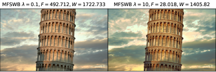
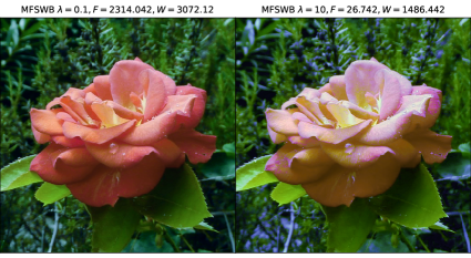
We first start with a simple simulation with 4 marginals which are empirical distributions with 100 i.i.d samples from 4 Gaussian distributions i.e., 𝒩((0,0),I)𝒩00𝐼\mathcal{N}((0,0),I), 𝒩((20,0),I)𝒩200𝐼\mathcal{N}((20,0),I), 𝒩((18,8),I)𝒩188𝐼\mathcal{N}((18,8),I), and 𝒩((18,8),I)𝒩188𝐼\mathcal{N}((18,-8),I). We then find the barycenter which is represented as an empirical distribution with 100 supports initialized by sampling i.i.d from 𝒩((0,5),I)𝒩05𝐼\mathcal{N}((0,-5),I). We use stochastic gradient descent with 50000 iterations of learning rate 0.01, the number of projections 100. We show the visualization of the found barycenters with the corresponding F-metric and W-metric by using USWB, s-MFSWB, us-MFSWB, and es-MFSWB at iterations 0, 1000, 5000, and 50000 in Figure 2. We observe that the USWB does not lead to a marginal fairness barycenter. The three proposed surrogate problems help to find a better barycenter faster in both two metrics than USWB. At convergence i.e., iteration 50000, we see that USWB does not give a fair barycenter while the three proposed surrogates lead to a more fair barycenter. Among the proposed surrogates, es-MFSWB gives the most marginal fairness barycenter with a competitive centerness. The formal MFSWB (dual form with λ=1𝜆1\lambda=1) leads to the most fair barycenter. However, the performance of the formal MFSWB is quite sensitive to λ𝜆\lambda. We show the visualization for λ=0.1𝜆0.1\lambda=0.1 and λ=10𝜆10\lambda=10 in Figure 5 in Appendix D.

4.2 3D Point-cloud Averaging

Refer to caption
Refer to caption
Figure 3: Averaging point-clouds with USWB, MFSWB (λ=1𝜆1\lambda=1), s-MFSWB, us-MFSWB, and es-MFSWB.
Table 1: F-metric and W-metric along iterations in point-cloud averaging application.
Method Iteration 0 Iteration 1000 Iteration 5000 Iteration 10000
F (\downarrow) W (\downarrow) F (\downarrow) W (\downarrow) F (\downarrow) W (\downarrow) F (\downarrow) W (\downarrow)
USWB 252.24±0.0plus-or-minus252.240.0252.24\pm 0.0 3746.05±0.0plus-or-minus3746.050.03746.05\pm 0.0 4.89±0.28plus-or-minus4.890.284.89\pm 0.28 85.72±0.18plus-or-minus85.720.1885.72\pm 0.18 3.79±0.32plus-or-minus3.790.323.79\pm 0.32 45.37±0.18plus-or-minus45.370.1845.37\pm 0.18 1.55±0.48plus-or-minus1.550.481.55\pm 0.48 39.81±0.18plus-or-minus39.810.1839.81\pm 0.18
MFSWB λ=0.1𝜆0.1\lambda=0.1 252.24±0.0plus-or-minus252.240.0252.24\pm 0.0 3746.05±0.0plus-or-minus3746.050.03746.05\pm 0.0 4.76±0.27plus-or-minus4.760.274.76\pm 0.27 84.86±0.17plus-or-minus84.860.1784.86\pm 0.17 3.78±0.2plus-or-minus3.780.23.78\pm 0.2 45.2±0.11plus-or-minus45.20.1145.2\pm 0.11 1.32±0.22plus-or-minus1.320.221.32\pm 0.22 39.73±0.16plus-or-minus39.730.1639.73\pm 0.16
MFSWB λ=1𝜆1\lambda=1 252.24±0.0plus-or-minus252.240.0252.24\pm 0.0 3746.05±0.0plus-or-minus3746.050.03746.05\pm 0.0 0.49±0.2plus-or-minus0.490.20.49\pm 0.2 79.08±0.15plus-or-minus79.080.1579.08\pm 0.15 3.64±0.26plus-or-minus3.640.263.64\pm 0.26 44.71±0.19plus-or-minus44.710.1944.71\pm 0.19 1.03±0.06plus-or-minus1.030.061.03\pm 0.06 39.45±0.18plus-or-minus39.450.1839.45\pm 0.18
MFSWB λ=10𝜆10\lambda=10 252.24±0.0plus-or-minus252.240.0252.24\pm 0.0 3746.05±0.0plus-or-minus3746.050.03746.05\pm 0.0 4.03±2.43plus-or-minus4.032.434.03\pm 2.43 71.24±0.9plus-or-minus71.240.9\mathbf{71.24\pm 0.9} 7.32±2.5plus-or-minus7.322.57.32\pm 2.5 45.21±0.2plus-or-minus45.210.245.21\pm 0.2 4.13±2.48plus-or-minus4.132.484.13\pm 2.48 42.56±0.36plus-or-minus42.560.3642.56\pm 0.36
s-MFSWB 252.24±0.0plus-or-minus252.240.0252.24\pm 0.0 3746.05±0.0plus-or-minus3746.050.03746.05\pm 0.0 2.52±0.77plus-or-minus2.520.772.52\pm 0.77 81.84±0.14plus-or-minus81.840.1481.84\pm 0.14 4.01±0.38plus-or-minus4.010.384.01\pm 0.38 44.9±0.13plus-or-minus44.90.1344.9\pm 0.13 1.15±0.09plus-or-minus1.150.091.15\pm 0.09 39.58±0.17plus-or-minus39.580.1739.58\pm 0.17
us-MFSWB 252.24±0.0plus-or-minus252.240.0252.24\pm 0.0 3746.05±0.0plus-or-minus3746.050.03746.05\pm 0.0 0.3±0.18plus-or-minus0.30.180.3\pm 0.18 78.69±0.17plus-or-minus78.690.1778.69\pm 0.17 3.74±0.26plus-or-minus3.740.263.74\pm 0.26 44.38±0.1plus-or-minus44.380.144.38\pm 0.1 0.87±0.18plus-or-minus0.870.180.87\pm 0.18 39.26±0.1plus-or-minus39.260.139.26\pm 0.1
es-MFSWB 252.24±0.0plus-or-minus252.240.0252.24\pm 0.0 3746.05±0.0plus-or-minus3746.050.03746.05\pm 0.0 0.2±0.19plus-or-minus0.20.19\mathbf{0.2\pm 0.19} 78.1±0.16plus-or-minus78.10.1678.1\pm 0.16 3.5±0.29plus-or-minus3.50.29\mathbf{3.5\pm 0.29} 44.37±0.08plus-or-minus44.370.08\mathbf{44.37\pm 0.08} 0.84±0.22plus-or-minus0.840.22\mathbf{0.84\pm 0.22} 39.18±0.08plus-or-minus39.180.08\mathbf{39.18\pm 0.08}

We aim to find the mean shape of point-cloud shapes by casting a point cloud X={x1,,xn}𝑋subscript𝑥1subscript𝑥𝑛X=\{x_{1},\ldots,x_{n}\} into an empirical probability measures PX=1ni=1nδxisubscript𝑃𝑋1𝑛superscriptsubscript𝑖1𝑛subscript𝛿subscript𝑥𝑖P_{X}=\frac{1}{n}\sum_{i=1}^{n}\delta_{x_{i}}. We select two point-cloud shapes which consist of 2048 points in ShapeNet Core-55 dataset [6]. We initialize the barycenter with a spherical point-cloud. We use stochastic gradient descent with 10000 iterations of learning rate 0.01, the number of projections 10. We report the found barycenters for two car shapes in Figure 3 at the final iteration and the corresponding F-metric and W-metric at iterations 0, 1000, 5000, and 10000 in Table 1 from three independent runs. As in the Gaussian simulation, s-MFSWB, us-MFSWB, and es-MFSWB help to reduce the two metrics faster than the USWB. With the slicing distribution selection, es-MFSWB performs the best at every iteration, even better than the formal MFSWB with three choices of λ𝜆\lambda i.e., 0.1,1,100.11100.1,1,10. We also observe a similar phenomenon for two plane shapes in Figure 6 and Table 3 in Appendix D. We refer the reader to Appendix D for a detailed discussion.

4.3 Color Harmonization

Refer to caption
Refer to caption
Figure 4: Harmonized images from USWB, MFSWB (λ=1𝜆1\lambda=1) s-MFSWB, us-MFSWB, and es-MFSWB.

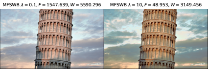
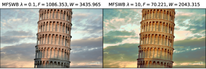
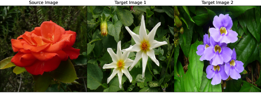
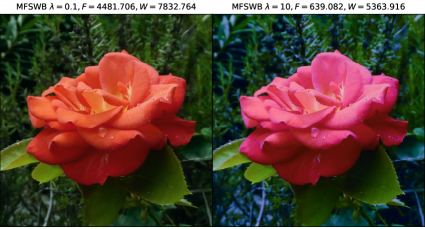
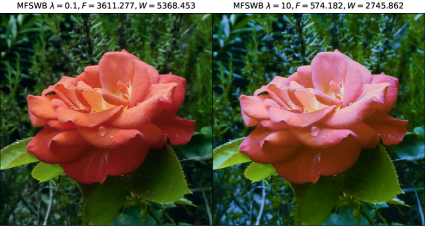
We want to transform the color palette of a source image, denoted as X=(x1,,xn)𝑋subscript𝑥1subscript𝑥𝑛X=(x_{1},\ldots,x_{n}) for n𝑛n is the number of pixels, to be an exact hybrid between two target images. Similar to the previous point-cloud averaging, we transform the color palette of an image into the empirical probability measure over colors (RGB) i.e., PX=1ni=1nδxisubscript𝑃𝑋1𝑛superscriptsubscript𝑖1𝑛subscript𝛿subscript𝑥𝑖P_{X}=\frac{1}{n}\sum_{i=1}^{n}\delta_{x_{i}}. We then minimize barycenter losses i.e., USWB, MFSWB (λ{0.1,1,10}𝜆0.1110\lambda\in\{0.1,1,10\}), s-MFSWB, us-MFSWB, and es-MFSWB by using stochastic gradient descent with the learning rate 0.00010.00010.0001 and 20000 iterations. We report both the transformed images and the corresponding F-metric and W-metric in Figure 4. We also report the full results in Figure 79 in Appendix D. As in previous experiments, we see that the three proposed surrogates yield a better barycenter faster than USWB. The proposed es-MFSWB is the best variant among all surrogates since it has the lowest F-metric and W-metric at all iterations. We refer the reader to Figure 10-Figure 13 in Appendix D for additional flowers-images example, where a similar relative comparison happens. For the formal MFSWB, it is worse than es-MFSWB in one setting and better than es-MFSWB in one setting with the right choice of λ𝜆\lambda. Therefore, it is more convenient to use us-MFSWB in practice.

4.4 Sliced Wasserstein Autoencoder with Class-Fair Representation

Problem. We consider training the sliced Wasserstein autoencoder (SWAE)[22] with a class-fairness regularization. In particular, we have the data distributions of K1𝐾1K\geq 1 classes i.e., μk𝒫(d)subscript𝜇𝑘𝒫superscript𝑑\mu_{k}\in\mathcal{P}(\mathbb{R}^{d}) for k=1,,K𝑘1𝐾k=1,\ldots,K and we would like to estimate an encoder network fϕ:dh:subscript𝑓italic-ϕsuperscript𝑑superscriptf_{\phi}:\mathbb{R}^{d}\to\mathbb{R}^{h} (ϕΦitalic-ϕΦ\phi\in\Phi) and a decoder network gψ:hd:subscript𝑔𝜓superscriptsuperscript𝑑g_{\psi}:\mathbb{R}^{h}\to\mathbb{R}^{d} (ψΨ𝜓Ψ\psi\in\Psi with hsuperscript\mathbb{R}^{h} is a low-dimensional latent space. Given a prior distribution μ0𝒫(h)subscript𝜇0𝒫superscript\mu_{0}\in\mathcal{P}(\mathbb{R}^{h}), p1𝑝1p\geq 1, κ1+subscript𝜅1superscript\kappa_{1}\in\mathbb{R}^{+}, κ2+subscript𝜅2superscript\kappa_{2}\in\mathbb{R}^{+}, and a minibatch size M1𝑀1M\geq 1, we perform the following optimization problem:

minϕ,ψ𝔼[1KMk=1Ki=1Mc(Xki,gψ(fϕ(Xki))+κ1SWpp(PZ,P(fϕ(Xk))k=1K)+κ2(PZ;Pf(X1):Pf(XK))],\displaystyle\min_{\phi,\psi}\mathbb{E}\left[\frac{1}{KM}\sum_{k=1}^{K}\sum_{i=1}^{M}c(X_{ki},g_{\psi}(f_{\phi}(X_{ki}))+\kappa_{1}SW_{p}^{p}(P_{Z},P_{(f_{\phi}(X_{k}))_{k=1}^{K}})+\kappa_{2}\mathcal{B}(P_{Z};P_{f(X_{1})}:P_{f(X_{K})})\right],

where (X1,,XK)μ1MμKMsimilar-tosubscript𝑋1subscript𝑋𝐾tensor-productsuperscriptsubscript𝜇1tensor-productabsent𝑀superscriptsubscript𝜇𝐾tensor-productabsent𝑀(X_{1},\ldots,X_{K})\sim\mu_{1}^{\otimes M}\otimes\ldots\otimes\mu_{K}^{\otimes M}, Zμ0Msimilar-to𝑍superscriptsubscript𝜇0tensor-productabsent𝑀Z\sim\mu_{0}^{\otimes M}, c𝑐c is a reconstruction loss, PZ=1Mi=1MδZisubscript𝑃𝑍1𝑀superscriptsubscript𝑖1𝑀subscript𝛿subscript𝑍𝑖P_{Z}=\frac{1}{M}\sum_{i=1}^{M}\delta_{Z_{i}}, P(fϕ(Xk))k=1K=1KMk=1Ki=1Mδfϕ(Xki)subscript𝑃superscriptsubscriptsubscript𝑓italic-ϕsubscript𝑋𝑘𝑘1𝐾1𝐾𝑀superscriptsubscript𝑘1𝐾superscriptsubscript𝑖1𝑀subscript𝛿subscript𝑓italic-ϕsubscript𝑋𝑘𝑖P_{(f_{\phi}(X_{k}))_{k=1}^{K}}=\frac{1}{KM}\sum_{k=1}^{K}\sum_{i=1}^{M}\delta_{f_{\phi}(X_{ki})}, Pf(Xk)=1Mi=1MδXkisubscript𝑃𝑓subscript𝑋𝑘1𝑀superscriptsubscript𝑖1𝑀subscript𝛿subscript𝑋𝑘𝑖P_{f(X_{k})}=\frac{1}{M}\sum_{i=1}^{M}\delta_{X_{ki}} for k=1,,K𝑘1𝐾k=1,\ldots,K, and \mathcal{B} denotes a barycenter loss i.e., USWB, MFSWB, s-MFSWB, us-MFSWB, and es-MFSWB. This setting can be seen as an inverse barycenter problem i.e., the barycenter is fixed and the marginals are learnt under some constraints (e.g., the reconstruction loss and the aggregated distribution loss).

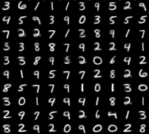
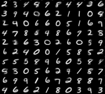
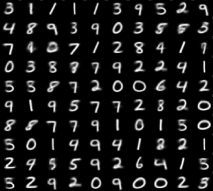
Results. We train the autoencoder on MNIST dataset [26] (d=28×28𝑑2828d=28\times 28) with κ1=8.0subscript𝜅18.0\kappa_{1}=8.0, κ2=0.5subscript𝜅20.5\kappa_{2}=0.5, 250 epochs, and μ0subscript𝜇0\mu_{0} is the uniform distribution on 2D ball (h=22h=2). We refer the reader to Appendix D for more details of the neural network architectures and the optimizer. Following the training phase, we evaluate the trained autoencoders on the MNIST test set. Similar to previous experiments, we use the metrics F (denoted as Flatentsubscript𝐹latentF_{\text{latent}}) and W (denoted as Wlatentsubscript𝑊latentW_{\text{latent}}) in the latent space distributions fϕμ1,,fϕμKsubscript𝑓italic-ϕsubscript𝜇1subscript𝑓italic-ϕsubscript𝜇𝐾f_{\phi}\sharp\mu_{1},\ldots,f_{\phi}\sharp\mu_{K} and the barycenter μ0subscript𝜇0\mu_{0}. We use the reconstruction loss (binary cross-entropy, denoted as RL), the Wasserstein-2 distance between the prior and aggregated posterior distribution in latent space W2,latent2:=W22(μ0,1Kk=1Kfϕμk)assignsuperscriptsubscriptW2latent2superscriptsubscript𝑊22subscript𝜇01𝐾superscriptsubscript𝑘1𝐾subscript𝑓italic-ϕsubscript𝜇𝑘\text{W}_{2,\text{latent}}^{2}:=W_{2}^{2}\left(\mu_{0},\frac{1}{K}\sum_{k=1}^{K}f_{\phi}\sharp\mu_{k}\right), as well as in image space W2,image2:=W22(gψμ0,1Kk=1Kμk)assignsuperscriptsubscriptW2image2superscriptsubscript𝑊22subscript𝑔𝜓subscript𝜇01𝐾superscriptsubscript𝑘1𝐾subscript𝜇𝑘\text{W}_{2,\text{image}}^{2}:=W_{2}^{2}\left(g_{\psi}\sharp\mu_{0},\frac{1}{K}\sum_{k=1}^{K}\mu_{k}\right). During evaluation, we approximate μ0subscript𝜇0\mu_{0} by its empirical version of 10000 samples. We report the quantitative result in Table 2, and reconstructed images, generated images, and images of latent codes in Figure 14 in Appendix D. From the results, we see that the proposed surrogate MFSWB yield better scores than USWB in all metrics except the generative score i.e., W2,image2superscriptsubscriptW2image2\text{W}_{2,\text{image}}^{2}. The formal MFSWB gives good score in reconstruction loss, W2,image2superscriptsubscriptW2image2\text{W}_{2,\text{image}}^{2}, and W2,latent2superscriptsubscriptW2latent2\text{W}_{2,\text{latent}}^{2}, however, its F and W scores are high. The es-MFSWB is the best variant among the proposed surrogates. Compared with the conventional SWAE, using a barycenter loss leads to a more class-fair latent representation, however, it sacrifices the image reconstructive and generative quality.

Table 2: Results of training SWAE with different regularization losses.
Methods RL (\downarrow) W2,latent2×102superscriptsubscriptW2latent2superscript102\text{W}_{2,\text{latent}}^{2}\times 10^{2}(\downarrow) W2,image2superscriptsubscriptW2image2\text{W}_{2,\text{image}}^{2} (\downarrow) Flatent×102subscriptFlatentsuperscript102\text{F}_{\text{latent}}\times 10^{2} (\downarrow) Wlatent×102subscriptWlatentsuperscript102\text{W}_{\text{latent}}\times 10^{2} (\downarrow)
SWAE 2.95 9.41 26.91 7.05 23.86
USWB 3.15 10.46 27.41 7.02 12.73
MFSWB λ=0.1𝜆0.1\lambda=0.1 3.11 8.52 26.62 8.66 20.01
MFSWB λ=1.0𝜆1.0\lambda=1.0 3.12 9.71 26.92 10.15 21.16
MFSWB λ=10.0𝜆10.0\lambda=10.0 2.79 10.32 26.95 8.27 23.39
s-MFSWB 3.22 10.50 28.69 1.30 13.71
us-MFSWB 3.05 7.79 27.81 2.29 9.11
es-MFSWB 3.35 9.60 28.27 0.98 9.92

5 Conclusion

We introduced marginal fairness sliced Wasserstein barycenter (MFSWB), a special case of sliced Wasserstein barycenter (SWB) which has approximately the same distance to marginals. We first defined the MFSWB as a constrainted uniform SWB problem. After that, to overcome the computational drawbacks of the original problem, we propose three surrogate definitions of MFSWB which are hyperparameter-free and easy to compute. We discussed the relationship of the proposed surrogate problems and their connection to the sliced Multi-marginal Wasserstein distance with the maximal ground metric. Finally, we conduct simulations with Gaussian and experiments on 3D point-cloud averaging, color harmonization, and sliced Wasserstein autoencoder with class-fairness representation to show the benefits of the proposed surrogate MFSWB definitions.

Acknowledgements

We would like to thank Joydeep Ghosh for his insightful discussion during the course of this project.

Supplement to “Marginal Fairness Sliced Wasserstein Barycenter"

We present skipped proofs in Appendix A. We then provide some additional materials which are mentioned in the main paper in Appendix B. After that, related works are discussed in Appendix C. We then provide additional experimental results in Appendix D. Finally, we report the used computational devices in Appendix E.

Appendix A Proofs

A.1 Proof of Proposition 1

Proof. From Definition 2, we have

𝒮(μ,μ1:K)𝒮𝜇subscript𝜇:1𝐾\displaystyle\mathcal{SF}(\mu,\mu_{1:K}) =maxk{1,,K}SWpp(μ,μk)absentsubscript𝑘1𝐾𝑆superscriptsubscript𝑊𝑝𝑝𝜇subscript𝜇𝑘\displaystyle=\max_{k\in\{1,\ldots,K\}}SW_{p}^{p}(\mu,\mu_{k})
=maxk{1,,K}𝔼θ𝒰(𝕊d1)[Wpp(θμ,θμk)]absentsubscript𝑘1𝐾subscript𝔼similar-to𝜃𝒰superscript𝕊𝑑1delimited-[]superscriptsubscript𝑊𝑝𝑝𝜃𝜇𝜃subscript𝜇𝑘\displaystyle=\max_{k\in\{1,\ldots,K\}}\mathbb{E}_{\theta\sim\mathcal{U}(\mathbb{S}^{d-1})}[W_{p}^{p}(\theta\sharp\mu,\theta\sharp\mu_{k})]

Let k=argmaxk{1,,K}𝔼θ𝒰(𝕊d1)[Wpp(θμ,θμk)]superscript𝑘subscriptargmax𝑘1𝐾subscript𝔼similar-to𝜃𝒰superscript𝕊𝑑1delimited-[]superscriptsubscript𝑊𝑝𝑝𝜃𝜇𝜃subscript𝜇𝑘k^{\star}=\operatorname*{arg\,max}_{k\in\{1,\ldots,K\}}\mathbb{E}_{\theta\sim\mathcal{U}(\mathbb{S}^{d-1})}[W_{p}^{p}(\theta\sharp\mu,\theta\sharp\mu_{k})], we have

𝒮(μ,μ1:K)𝒮𝜇subscript𝜇:1𝐾\displaystyle\mathcal{SF}(\mu,\mu_{1:K}) =𝔼θ𝒰(𝕊d1)[Wpp(θμ,θμk)]absentsubscript𝔼similar-to𝜃𝒰superscript𝕊𝑑1delimited-[]superscriptsubscript𝑊𝑝𝑝𝜃𝜇𝜃subscript𝜇superscript𝑘\displaystyle=\mathbb{E}_{\theta\sim\mathcal{U}(\mathbb{S}^{d-1})}[W_{p}^{p}(\theta\sharp\mu,\theta\sharp\mu_{k^{\star}})]
𝔼θ𝒰(𝕊d1)[maxk{1,,K}Wpp(θμ,θμk)]absentsubscript𝔼similar-to𝜃𝒰superscript𝕊𝑑1delimited-[]subscript𝑘1𝐾superscriptsubscript𝑊𝑝𝑝𝜃𝜇𝜃subscript𝜇𝑘\displaystyle\leq\mathbb{E}_{\theta\sim\mathcal{U}(\mathbb{S}^{d-1})}\left[\max_{k\in\{1,\ldots,K\}}W_{p}^{p}(\theta\sharp\mu,\theta\sharp\mu_{k})\right]
=𝒰𝒮(μ,μ1:K),absent𝒰𝒮𝜇subscript𝜇:1𝐾\displaystyle=\mathcal{USF}(\mu,\mu_{1:K}),

as from Definition 3, which completes the proof.

A.2 Proof of Proposition 2

Using the Holder’s inequality, we have:

𝔼|ϕ1Ll=1LWpp(θlμϕ,θlμkθl)ϕ𝒰𝒮(μϕ;μ1:K)|𝔼subscriptitalic-ϕ1𝐿superscriptsubscript𝑙1𝐿superscriptsubscriptW𝑝𝑝subscript𝜃𝑙subscript𝜇italic-ϕsubscript𝜃𝑙subscript𝜇subscriptsuperscript𝑘subscript𝜃𝑙subscriptitalic-ϕ𝒰𝒮subscript𝜇italic-ϕsubscript𝜇:1𝐾\displaystyle\mathbb{E}\left|\nabla_{\phi}\frac{1}{L}\sum_{l=1}^{L}\text{W}_{p}^{p}(\theta_{l}\sharp\mu_{\phi},\theta_{l}\sharp\mu_{k^{\star}_{\theta_{l}}})-\nabla_{\phi}\mathcal{USF}(\mu_{\phi};\mu_{1:K})\right|
(𝔼|ϕ1Ll=1LWpp(θlμϕ,θlμkθl)ϕ𝒰𝒮(μϕ;μ1:K)|2)12absentsuperscript𝔼superscriptsubscriptitalic-ϕ1𝐿superscriptsubscript𝑙1𝐿superscriptsubscriptW𝑝𝑝subscript𝜃𝑙subscript𝜇italic-ϕsubscript𝜃𝑙subscript𝜇subscriptsuperscript𝑘subscript𝜃𝑙subscriptitalic-ϕ𝒰𝒮subscript𝜇italic-ϕsubscript𝜇:1𝐾212\displaystyle\leq\left(\mathbb{E}\left|\nabla_{\phi}\frac{1}{L}\sum_{l=1}^{L}\text{W}_{p}^{p}(\theta_{l}\sharp\mu_{\phi},\theta_{l}\sharp\mu_{k^{\star}_{\theta_{l}}})-\nabla_{\phi}\mathcal{USF}(\mu_{\phi};\mu_{1:K})\right|^{2}\right)^{\frac{1}{2}}
=(𝔼(ϕ1Ll=1LWpp(θlμϕ,θlμkθl)ϕ𝔼[Wpp(θμϕ,θμkθ)])2)12absentsuperscript𝔼superscriptsubscriptitalic-ϕ1𝐿superscriptsubscript𝑙1𝐿superscriptsubscriptW𝑝𝑝subscript𝜃𝑙subscript𝜇italic-ϕsubscript𝜃𝑙subscript𝜇subscriptsuperscript𝑘subscript𝜃𝑙subscriptitalic-ϕ𝔼delimited-[]superscriptsubscriptW𝑝𝑝𝜃subscript𝜇italic-ϕ𝜃subscript𝜇subscriptsuperscript𝑘𝜃212\displaystyle=\left(\mathbb{E}\left(\nabla_{\phi}\frac{1}{L}\sum_{l=1}^{L}\text{W}_{p}^{p}(\theta_{l}\sharp\mu_{\phi},\theta_{l}\sharp\mu_{k^{\star}_{\theta_{l}}})-\nabla_{\phi}\mathbb{E}\left[\text{W}_{p}^{p}(\theta\sharp\mu_{\phi},\theta\sharp\mu_{k^{\star}_{\theta}})\right]\right)^{2}\right)^{\frac{1}{2}}
=(𝔼(1Ll=1LϕWpp(θlμϕ,θlμkθl)𝔼[ϕWpp(θμϕ,θμkθ)])2)12absentsuperscript𝔼superscript1𝐿superscriptsubscript𝑙1𝐿subscriptitalic-ϕsuperscriptsubscriptW𝑝𝑝subscript𝜃𝑙subscript𝜇italic-ϕsubscript𝜃𝑙subscript𝜇subscriptsuperscript𝑘subscript𝜃𝑙𝔼delimited-[]subscriptitalic-ϕsuperscriptsubscriptW𝑝𝑝𝜃subscript𝜇italic-ϕ𝜃subscript𝜇subscriptsuperscript𝑘𝜃212\displaystyle=\left(\mathbb{E}\left(\frac{1}{L}\sum_{l=1}^{L}\nabla_{\phi}\text{W}_{p}^{p}(\theta_{l}\sharp\mu_{\phi},\theta_{l}\sharp\mu_{k^{\star}_{\theta_{l}}})-\mathbb{E}\left[\nabla_{\phi}\text{W}_{p}^{p}(\theta\sharp\mu_{\phi},\theta\sharp\mu_{k^{\star}_{\theta}})\right]\right)^{2}\right)^{\frac{1}{2}}
=(Var[1Ll=1LϕWpp(θlμϕ,θlμkθl)])12absentsuperscriptVardelimited-[]1𝐿superscriptsubscript𝑙1𝐿subscriptitalic-ϕsuperscriptsubscriptW𝑝𝑝subscript𝜃𝑙subscript𝜇italic-ϕsubscript𝜃𝑙subscript𝜇subscriptsuperscript𝑘subscript𝜃𝑙12\displaystyle=\left(\text{Var}\left[\frac{1}{L}\sum_{l=1}^{L}\nabla_{\phi}\text{W}_{p}^{p}(\theta_{l}\sharp\mu_{\phi},\theta_{l}\sharp\mu_{k^{\star}_{\theta_{l}}})\right]\right)^{\frac{1}{2}}
=1LVar[ϕWpp(θμϕ,θμkθ)]12,absent1𝐿Varsuperscriptdelimited-[]subscriptitalic-ϕsuperscriptsubscriptW𝑝𝑝𝜃subscript𝜇italic-ϕ𝜃subscript𝜇subscriptsuperscript𝑘𝜃12\displaystyle=\frac{1}{\sqrt{L}}\text{Var}\left[\nabla_{\phi}\text{W}_{p}^{p}(\theta\sharp\mu_{\phi},\theta\sharp\mu_{k^{\star}_{\theta}})\right]^{\frac{1}{2}},

which completes the proof.

A.3 Proof of Proposition 3

We first restate the following Lemma from [36] and provide the proof for completeness.

Lemma 1.

For any L1𝐿1L\geq 1, 0a1a2aL0subscript𝑎1subscript𝑎2subscript𝑎𝐿0\leq a_{1}\leq a_{2}\leq\ldots\leq a_{L} and 0<b1b2bL0subscript𝑏1subscript𝑏2subscript𝑏𝐿0<b_{1}\leq b_{2}\leq\ldots\leq b_{L}, we have:

1L(i=1Lai)(i=1Lbi)i=1Laibi.1𝐿superscriptsubscript𝑖1𝐿subscript𝑎𝑖superscriptsubscript𝑖1𝐿subscript𝑏𝑖superscriptsubscript𝑖1𝐿subscript𝑎𝑖subscript𝑏𝑖\displaystyle\frac{1}{L}(\sum_{i=1}^{L}a_{i})(\sum_{i=1}^{L}b_{i})\leq\sum_{i=1}^{L}a_{i}b_{i}. (15)
Proof.

For L=1𝐿1L=1, we directly have aibi=aibisubscript𝑎𝑖subscript𝑏𝑖subscript𝑎𝑖subscript𝑏𝑖a_{i}b_{i}=a_{i}b_{i}. Assuming that for L𝐿L the inequality holds i.e., 1L(i=1Lai)(i=1Lbi)i=1Laibi1𝐿superscriptsubscript𝑖1𝐿subscript𝑎𝑖superscriptsubscript𝑖1𝐿subscript𝑏𝑖superscriptsubscript𝑖1𝐿subscript𝑎𝑖subscript𝑏𝑖\frac{1}{L}(\sum_{i=1}^{L}a_{i})(\sum_{i=1}^{L}b_{i})\leq\sum_{i=1}^{L}a_{i}b_{i} which is equivalent to (i=1Lai)(i=1Lbi)Li=1Laibi.superscriptsubscript𝑖1𝐿subscript𝑎𝑖superscriptsubscript𝑖1𝐿subscript𝑏𝑖𝐿superscriptsubscript𝑖1𝐿subscript𝑎𝑖subscript𝑏𝑖(\sum_{i=1}^{L}a_{i})(\sum_{i=1}^{L}b_{i})\leq L\sum_{i=1}^{L}a_{i}b_{i}. Now, we show that 1L(i=1Lai)(i=1Lbi)i=1Laibi1𝐿superscriptsubscript𝑖1𝐿subscript𝑎𝑖superscriptsubscript𝑖1𝐿subscript𝑏𝑖superscriptsubscript𝑖1𝐿subscript𝑎𝑖subscript𝑏𝑖\frac{1}{L}(\sum_{i=1}^{L}a_{i})(\sum_{i=1}^{L}b_{i})\leq\sum_{i=1}^{L}a_{i}b_{i} i.e., the inequality holds for L+1𝐿1L+1. We have

(i=1L+1ai)(i=1L+1bi)superscriptsubscript𝑖1𝐿1subscript𝑎𝑖superscriptsubscript𝑖1𝐿1subscript𝑏𝑖\displaystyle(\sum_{i=1}^{L+1}a_{i})(\sum_{i=1}^{L+1}b_{i}) =(i=1Lai)(i=1Lbi)+(i=1Lai)bL+1+(i=1Lbi)aL+1+aL+1bL+1absentsuperscriptsubscript𝑖1𝐿subscript𝑎𝑖superscriptsubscript𝑖1𝐿subscript𝑏𝑖superscriptsubscript𝑖1𝐿subscript𝑎𝑖subscript𝑏𝐿1superscriptsubscript𝑖1𝐿subscript𝑏𝑖subscript𝑎𝐿1subscript𝑎𝐿1subscript𝑏𝐿1\displaystyle=(\sum_{i=1}^{L}a_{i})(\sum_{i=1}^{L}b_{i})+(\sum_{i=1}^{L}a_{i})b_{L+1}+(\sum_{i=1}^{L}b_{i})a_{L+1}+a_{L+1}b_{L+1}
Li=1Laibi+(i=1Lai)bL+1+(i=1Lbi)aL+1+aL+1bL+1.absent𝐿superscriptsubscript𝑖1𝐿subscript𝑎𝑖subscript𝑏𝑖superscriptsubscript𝑖1𝐿subscript𝑎𝑖subscript𝑏𝐿1superscriptsubscript𝑖1𝐿subscript𝑏𝑖subscript𝑎𝐿1subscript𝑎𝐿1subscript𝑏𝐿1\displaystyle\leq L\sum_{i=1}^{L}a_{i}b_{i}+(\sum_{i=1}^{L}a_{i})b_{L+1}+(\sum_{i=1}^{L}b_{i})a_{L+1}+a_{L+1}b_{L+1}.

Since aL+1bL+1+aibiaL+1bi+bL+1aisubscript𝑎𝐿1subscript𝑏𝐿1subscript𝑎𝑖subscript𝑏𝑖subscript𝑎𝐿1subscript𝑏𝑖subscript𝑏𝐿1subscript𝑎𝑖a_{L+1}b_{L+1}+a_{i}b_{i}\geq a_{L+1}b_{i}+b_{L+1}a_{i} for all 1iL1𝑖𝐿1\leq i\leq L by rearrangement inequality. By taking the sum of these inequalities over i𝑖i from 111 to L𝐿L, we obtain:

(i=1Lai)bL+1+(i=1Lbi)aL+1i=1Laibi+LaL+1bL+1.superscriptsubscript𝑖1𝐿subscript𝑎𝑖subscript𝑏𝐿1superscriptsubscript𝑖1𝐿subscript𝑏𝑖subscript𝑎𝐿1superscriptsubscript𝑖1𝐿subscript𝑎𝑖subscript𝑏𝑖𝐿subscript𝑎𝐿1subscript𝑏𝐿1\displaystyle(\sum_{i=1}^{L}a_{i})b_{L+1}+(\sum_{i=1}^{L}b_{i})a_{L+1}\leq\sum_{i=1}^{L}a_{i}b_{i}+La_{L+1}b_{L+1}.

Then, we have

(i=1L+1ai)(i=1L+1bi)superscriptsubscript𝑖1𝐿1subscript𝑎𝑖superscriptsubscript𝑖1𝐿1subscript𝑏𝑖\displaystyle(\sum_{i=1}^{L+1}a_{i})(\sum_{i=1}^{L+1}b_{i}) Li=1Laibi+(i=1Lai)bL+1+(i=1Lbi)aL+1+aL+1bL+1absent𝐿superscriptsubscript𝑖1𝐿subscript𝑎𝑖subscript𝑏𝑖superscriptsubscript𝑖1𝐿subscript𝑎𝑖subscript𝑏𝐿1superscriptsubscript𝑖1𝐿subscript𝑏𝑖subscript𝑎𝐿1subscript𝑎𝐿1subscript𝑏𝐿1\displaystyle\leq L\sum_{i=1}^{L}a_{i}b_{i}+(\sum_{i=1}^{L}a_{i})b_{L+1}+(\sum_{i=1}^{L}b_{i})a_{L+1}+a_{L+1}b_{L+1}
Li=1Laibi+i=1Laibi+LaL+1bL+1+aL+1bL+1absent𝐿superscriptsubscript𝑖1𝐿subscript𝑎𝑖subscript𝑏𝑖superscriptsubscript𝑖1𝐿subscript𝑎𝑖subscript𝑏𝑖𝐿subscript𝑎𝐿1subscript𝑏𝐿1subscript𝑎𝐿1subscript𝑏𝐿1\displaystyle\leq L\sum_{i=1}^{L}a_{i}b_{i}+\sum_{i=1}^{L}a_{i}b_{i}+La_{L+1}b_{L+1}+a_{L+1}b_{L+1}
=(L+1)(i=1L+1aibi),absent𝐿1superscriptsubscript𝑖1𝐿1subscript𝑎𝑖subscript𝑏𝑖\displaystyle=(L+1)(\sum_{i=1}^{L+1}a_{i}b_{i}),

which completes the proof. ∎

Now, we go back to the main inequality which is 𝒰𝒮(μ;μ1:K)𝒮(μ;μ1:K)𝒰𝒮𝜇subscript𝜇:1𝐾𝒮𝜇subscript𝜇:1𝐾\mathcal{USF}(\mu;\mu_{1:K})\leq\mathcal{ESF}(\mu;\mu_{1:K}). From Definition 5, we have:

𝒮(μ;μ1:K)𝒮𝜇subscript𝜇:1𝐾\displaystyle\mathcal{ESF}(\mu;\mu_{1:K}) =𝔼θσ(θ;μ,μ1:K)[maxk{1,,K}Wpp(θμ,θμk)]absentsubscript𝔼similar-to𝜃𝜎𝜃𝜇subscript𝜇:1𝐾delimited-[]subscript𝑘1𝐾superscriptsubscript𝑊𝑝𝑝𝜃𝜇𝜃subscript𝜇𝑘\displaystyle=\mathbb{E}_{\theta\sim\sigma(\theta;\mu,\mu_{1:K})}\left[\max_{k\in\{1,\ldots,K\}}W_{p}^{p}(\theta\sharp\mu,\theta\sharp\mu_{k})\right]
=𝔼θ𝒰(𝕊d1)[maxk{1,,K}Wpp(θμ,θμk)fσ(θ;μ,μ1:K)Γ(d/2)2πd/2],absentsubscript𝔼similar-to𝜃𝒰superscript𝕊𝑑1delimited-[]subscript𝑘1𝐾superscriptsubscript𝑊𝑝𝑝𝜃𝜇𝜃subscript𝜇𝑘subscript𝑓𝜎𝜃𝜇subscript𝜇:1𝐾Γ𝑑22superscript𝜋𝑑2\displaystyle=\mathbb{E}_{\theta\sim\mathcal{U}(\mathbb{S}^{d-1})}\left[\max_{k\in\{1,\ldots,K\}}W_{p}^{p}(\theta\sharp\mu,\theta\sharp\mu_{k})\frac{f_{\sigma}(\theta;\mu,\mu_{1:K})}{\frac{\Gamma(d/2)}{2\pi^{d/2}}}\right],

where fσ(θ;μ,μ1:K)exp(maxk{1,,K}Wpp(θμ,θμk))proportional-tosubscript𝑓𝜎𝜃𝜇subscript𝜇:1𝐾subscript𝑘1𝐾superscriptsubscript𝑊𝑝𝑝𝜃𝜇𝜃subscript𝜇𝑘f_{\sigma}(\theta;\mu,\mu_{1:K})\propto\exp\left(\max_{k\in\{1,\ldots,K\}}W_{p}^{p}(\theta\sharp\mu,\theta\sharp\mu_{k})\right). Now, we consider a Monte Carlo estimation of 𝒮(μ;μ1:K)𝒮𝜇subscript𝜇:1𝐾\mathcal{ESF}(\mu;\mu_{1:K}) by importance sampling:

𝒮^(μ;μ1:K,L)=1Ll=1L[maxk{1,,K}Wpp(θlμ,θlμk)exp(maxk{1,,K}Wpp(θlμ,θlμk))i=1Lexp(maxk{1,,K}Wpp(θiμ,θiμk))],^𝒮𝜇subscript𝜇:1𝐾𝐿1𝐿superscriptsubscript𝑙1𝐿delimited-[]subscript𝑘1𝐾superscriptsubscript𝑊𝑝𝑝subscript𝜃𝑙𝜇subscript𝜃𝑙subscript𝜇𝑘subscript𝑘1𝐾superscriptsubscript𝑊𝑝𝑝subscript𝜃𝑙𝜇subscript𝜃𝑙subscript𝜇𝑘superscriptsubscript𝑖1𝐿subscript𝑘1𝐾superscriptsubscript𝑊𝑝𝑝subscript𝜃𝑖𝜇subscript𝜃𝑖subscript𝜇𝑘\displaystyle\widehat{\mathcal{ESF}}(\mu;\mu_{1:K},L)=\frac{1}{L}\sum_{l=1}^{L}\left[\max_{k\in\{1,\ldots,K\}}W_{p}^{p}(\theta_{l}\sharp\mu,\theta_{l}\sharp\mu_{k})\frac{\exp\left(\max_{k\in\{1,\ldots,K\}}W_{p}^{p}(\theta_{l}\sharp\mu,\theta_{l}\sharp\mu_{k})\right)}{\sum_{i=1}^{L}\exp\left(\max_{k\in\{1,\ldots,K\}}W_{p}^{p}(\theta_{i}\sharp\mu,\theta_{i}\sharp\mu_{k})\right)}\right],

where θ1,,θLi.i.d𝒰(𝕊d1)subscript𝜃1subscript𝜃𝐿formulae-sequence𝑖𝑖𝑑similar-to𝒰superscript𝕊𝑑1\theta_{1},\ldots,\theta_{L}\overset{i.i.d}{\sim}\mathcal{U}(\mathbb{S}^{d-1}). Similarly, we consider a Monte Carlo estimation of 𝒰𝒮(μ;μ1:K)𝒰𝒮𝜇subscript𝜇:1𝐾\mathcal{USF}(\mu;\mu_{1:K}):

𝒰𝒮^(μ;μ1:K,L)=1Ll=1L[maxk{1,,K}Wpp(θlμ,θlμk)],^𝒰𝒮𝜇subscript𝜇:1𝐾𝐿1𝐿superscriptsubscript𝑙1𝐿delimited-[]subscript𝑘1𝐾superscriptsubscript𝑊𝑝𝑝subscript𝜃𝑙𝜇subscript𝜃𝑙subscript𝜇𝑘\displaystyle\widehat{\mathcal{USF}}(\mu;\mu_{1:K},L)=\frac{1}{L}\sum_{l=1}^{L}\left[\max_{k\in\{1,\ldots,K\}}W_{p}^{p}(\theta_{l}\sharp\mu,\theta_{l}\sharp\mu_{k})\right],

for the same set of θ1,,θLsubscript𝜃1subscript𝜃𝐿\theta_{1},\ldots,\theta_{L}. Without losing generality, we assume that maxk{1,,K}Wpp(θ1μ,θ1μk)maxk{1,,K}Wpp(θLμ,θLμk)subscript𝑘1𝐾superscriptsubscript𝑊𝑝𝑝subscript𝜃1𝜇subscript𝜃1subscript𝜇𝑘subscript𝑘1𝐾superscriptsubscript𝑊𝑝𝑝subscript𝜃𝐿𝜇subscript𝜃𝐿subscript𝜇𝑘\max_{k\in\{1,\ldots,K\}}W_{p}^{p}(\theta_{1}\sharp\mu,\theta_{1}\sharp\mu_{k})\leq\ldots\leq\max_{k\in\{1,\ldots,K\}}W_{p}^{p}(\theta_{L}\sharp\mu,\theta_{L}\sharp\mu_{k}).

Let maxk{1,,K}Wpp(θiμ,θiμk)=aisubscript𝑘1𝐾superscriptsubscript𝑊𝑝𝑝subscript𝜃𝑖𝜇subscript𝜃𝑖subscript𝜇𝑘subscript𝑎𝑖\max_{k\in\{1,\ldots,K\}}W_{p}^{p}(\theta_{i}\sharp\mu,\theta_{i}\sharp\mu_{k})=a_{i} and exp(maxk{1,,K}Wpp(θiμ,θiμk))=bisubscript𝑘1𝐾superscriptsubscript𝑊𝑝𝑝subscript𝜃𝑖𝜇subscript𝜃𝑖subscript𝜇𝑘subscript𝑏𝑖\exp\left(\max_{k\in\{1,\ldots,K\}}W_{p}^{p}(\theta_{i}\sharp\mu,\theta_{i}\sharp\mu_{k})\right)=b_{i}, applying Lemma 1, we have:

𝒰𝒮^(μ;μ1:K,L)𝒮^(μ;μ1:K,L)L1.formulae-sequence^𝒰𝒮𝜇subscript𝜇:1𝐾𝐿^𝒮𝜇subscript𝜇:1𝐾𝐿for-all𝐿1\displaystyle\widehat{\mathcal{USF}}(\mu;\mu_{1:K},L)\leq\widehat{\mathcal{ESF}}(\mu;\mu_{1:K},L)\quad\forall L\geq 1.

By letting L𝐿L\to\infty and applying the law of large numbers, we obtain:

𝒰𝒮(μ;μ1:K)𝒮(μ;μ1:K),𝒰𝒮𝜇subscript𝜇:1𝐾𝒮𝜇subscript𝜇:1𝐾\displaystyle\mathcal{USF}(\mu;\mu_{1:K})\leq\mathcal{ESF}(\mu;\mu_{1:K}),

which completes the proof.

A.4 Proof of Proposition 4

We first recall the definition of the SMW with the maximal ground metric:

SMWpp(μ1,,μK;c)𝑆𝑀superscriptsubscript𝑊𝑝𝑝subscript𝜇1subscript𝜇𝐾𝑐\displaystyle SMW_{p}^{p}(\mu_{1},\ldots,\mu_{K};c) =𝔼[infπΠ(μ1,,μK)maxi{1,,K},j{1,,K}|θxiθxj|pdπ(x1,,xK)].absent𝔼delimited-[]subscriptinfimum𝜋Πsubscript𝜇1subscript𝜇𝐾subscriptformulae-sequence𝑖1𝐾𝑗1𝐾superscriptsuperscript𝜃topsubscript𝑥𝑖superscript𝜃topsubscript𝑥𝑗𝑝𝑑𝜋subscript𝑥1subscript𝑥𝐾\displaystyle=\mathbb{E}\left[\inf_{\pi\in\Pi(\mu_{1},\ldots,\mu_{K})}\int\max_{i\in\{1,\ldots,K\},j\in\{1,\ldots,K\}}|\theta^{\top}x_{i}-\theta^{\top}x_{j}|^{p}d\pi(x_{1},\ldots,x_{K})\right].

Non-negativity. Since maxi{1,,K},j{1,,K}|θxiθxj|p0subscriptformulae-sequence𝑖1𝐾𝑗1𝐾superscriptsuperscript𝜃topsubscript𝑥𝑖superscript𝜃topsubscript𝑥𝑗𝑝0\max_{i\in\{1,\ldots,K\},j\in\{1,\ldots,K\}}|\theta^{\top}x_{i}-\theta^{\top}x_{j}|^{p}\geq 0 for any x1,,xKsubscript𝑥1subscript𝑥𝐾x_{1},\ldots,x_{K} and for any θ𝜃\theta, we can obtain the desired property SMWpp(μ1,,μK;c)0𝑆𝑀superscriptsubscript𝑊𝑝𝑝subscript𝜇1subscript𝜇𝐾𝑐0SMW_{p}^{p}(\mu_{1},\ldots,\mu_{K};c)\geq 0 which implies SMWp(μ1,,μK;c)0𝑆𝑀subscript𝑊𝑝subscript𝜇1subscript𝜇𝐾𝑐0SMW_{p}(\mu_{1},\ldots,\mu_{K};c)\geq 0.

Marginal Exchangeability. For any permutation σ:[[K]][[K]]:𝜎delimited-[]delimited-[]𝐾delimited-[]delimited-[]𝐾\sigma:[[K]]\to[[K]], we have:

SMWpp(μ1,,μK;c)𝑆𝑀superscriptsubscript𝑊𝑝𝑝subscript𝜇1subscript𝜇𝐾𝑐\displaystyle SMW_{p}^{p}(\mu_{1},\ldots,\mu_{K};c) =𝔼[infπΠ(μ1,,μK)maxi{1,,K},j{1,,K}|θxiθxj|pdπ(x1,,xK)]absent𝔼delimited-[]subscriptinfimum𝜋Πsubscript𝜇1subscript𝜇𝐾subscriptformulae-sequence𝑖1𝐾𝑗1𝐾superscriptsuperscript𝜃topsubscript𝑥𝑖superscript𝜃topsubscript𝑥𝑗𝑝𝑑𝜋subscript𝑥1subscript𝑥𝐾\displaystyle=\mathbb{E}\left[\inf_{\pi\in\Pi(\mu_{1},\ldots,\mu_{K})}\int\max_{i\in\{1,\ldots,K\},j\in\{1,\ldots,K\}}|\theta^{\top}x_{i}-\theta^{\top}x_{j}|^{p}d\pi(x_{1},\ldots,x_{K})\right]
=𝔼[infπΠ(μσ(1),,μσ(K))maxi{1,,K},j{1,,K}|θxiθxj|pdπ(x1,,xK)]absent𝔼delimited-[]subscriptinfimum𝜋Πsubscript𝜇𝜎1subscript𝜇𝜎𝐾subscriptformulae-sequence𝑖1𝐾𝑗1𝐾superscriptsuperscript𝜃topsubscript𝑥𝑖superscript𝜃topsubscript𝑥𝑗𝑝𝑑𝜋subscript𝑥1subscript𝑥𝐾\displaystyle=\mathbb{E}\left[\inf_{\pi\in\Pi(\mu_{\sigma(1)},\ldots,\mu_{\sigma(K)})}\int\max_{i\in\{1,\ldots,K\},j\in\{1,\ldots,K\}}|\theta^{\top}x_{i}-\theta^{\top}x_{j}|^{p}d\pi(x_{1},\ldots,x_{K})\right]
=SMWpp(μσ(1),,μσ(K);c).absent𝑆𝑀superscriptsubscript𝑊𝑝𝑝subscript𝜇𝜎1subscript𝜇𝜎𝐾𝑐\displaystyle=SMW_{p}^{p}(\mu_{\sigma(1)},\ldots,\mu_{\sigma(K)};c).

Generalized Triangle Inequality. For μ𝒫p(d)𝜇subscript𝒫𝑝superscript𝑑\mu\in\mathcal{P}_{p}(\mathbb{R}^{d}), we have :

SMWpp(μ1,,μK;c)𝑆𝑀superscriptsubscript𝑊𝑝𝑝subscript𝜇1subscript𝜇𝐾𝑐\displaystyle SMW_{p}^{p}(\mu_{1},\ldots,\mu_{K};c)
=𝔼[infπΠ(μ1,,μK)maxi{1,,K},j{1,,K}|θxiθxj|pdπ(x1,,xK)]absent𝔼delimited-[]subscriptinfimum𝜋Πsubscript𝜇1subscript𝜇𝐾subscriptformulae-sequence𝑖1𝐾𝑗1𝐾superscriptsuperscript𝜃topsubscript𝑥𝑖superscript𝜃topsubscript𝑥𝑗𝑝𝑑𝜋subscript𝑥1subscript𝑥𝐾\displaystyle=\mathbb{E}\left[\inf_{\pi\in\Pi(\mu_{1},\ldots,\mu_{K})}\int\max_{i\in\{1,\ldots,K\},j\in\{1,\ldots,K\}}|\theta^{\top}x_{i}-\theta^{\top}x_{j}|^{p}d\pi(x_{1},\ldots,x_{K})\right]
𝔼[infπΠ(μ1,,μK)k=1Kmaxi{1,,K}{k},j{1,,K}{k}|θxiθxj|pdπ(x1,,xK)]absent𝔼delimited-[]subscriptinfimum𝜋Πsubscript𝜇1subscript𝜇𝐾superscriptsubscript𝑘1𝐾subscriptformulae-sequence𝑖1𝐾𝑘𝑗1𝐾𝑘superscriptsuperscript𝜃topsubscript𝑥𝑖superscript𝜃topsubscript𝑥𝑗𝑝𝑑𝜋subscript𝑥1subscript𝑥𝐾\displaystyle\leq\mathbb{E}\left[\inf_{\pi\in\Pi(\mu_{1},\ldots,\mu_{K})}\int\sum_{k=1}^{K}\max_{i\in\{1,\ldots,K\}\setminus\{{k}\},j\in\{1,\ldots,K\}\setminus\{{k}\}}|\theta^{\top}x_{i}-\theta^{\top}x_{j}|^{p}d\pi(x_{1},\ldots,x_{K})\right]
=𝔼[infπΠ(μ1,,μK)k=1Kmaxi{1,,K}{k},j{1,,K}{k}|θxiθxj|pdπ(x1,,xK)]absent𝔼delimited-[]subscriptinfimum𝜋Πsubscript𝜇1subscript𝜇𝐾superscriptsubscript𝑘1𝐾subscriptformulae-sequence𝑖1𝐾𝑘𝑗1𝐾𝑘superscriptsuperscript𝜃topsubscript𝑥𝑖superscript𝜃topsubscript𝑥𝑗𝑝𝑑𝜋subscript𝑥1subscript𝑥𝐾\displaystyle=\mathbb{E}\left[\inf_{\pi\in\Pi(\mu_{1},\ldots,\mu_{K})}\sum_{k=1}^{K}\int\max_{i\in\{1,\ldots,K\}\setminus\{{k}\},j\in\{1,\ldots,K\}\setminus\{{k}\}}|\theta^{\top}x_{i}-\theta^{\top}x_{j}|^{p}d\pi(x_{1},\ldots,x_{K})\right]
=𝔼[k=1Kmaxi{1,,K}{k},j{1,,K}{k}|θxiθxj|pdπ(x1,,xk1,xk+1,xK)]absent𝔼delimited-[]superscriptsubscript𝑘1𝐾subscriptformulae-sequence𝑖1𝐾𝑘𝑗1𝐾𝑘superscriptsuperscript𝜃topsubscript𝑥𝑖superscript𝜃topsubscript𝑥𝑗𝑝𝑑superscript𝜋subscript𝑥1subscript𝑥𝑘1subscript𝑥𝑘1subscript𝑥𝐾\displaystyle=\mathbb{E}\left[\sum_{k=1}^{K}\int\max_{i\in\{1,\ldots,K\}\setminus\{{k}\},j\in\{1,\ldots,K\}\setminus\{{k}\}}|\theta^{\top}x_{i}-\theta^{\top}x_{j}|^{p}d\pi^{\star}(x_{1},\ldots,x_{k-1},x_{k+1},\ldots x_{K})\right]

for πsuperscript𝜋\pi^{\star} is the optimal multi-marginal transportation plan and π(x1,,xk1,xk+1,xK)superscript𝜋subscript𝑥1subscript𝑥𝑘1subscript𝑥𝑘1subscript𝑥𝐾\pi^{\star}(x_{1},\ldots,x_{k-1},x_{k+1},x_{K}\ ) is the marginal joint distribution by integrating out xksubscript𝑥𝑘x_{k}. By the gluing lemma [38], there exists optimal plans π(x1,,xk1,y,xk+1,xK)superscript𝜋subscript𝑥1subscript𝑥𝑘1𝑦subscript𝑥𝑘1subscript𝑥𝐾\pi^{\star}(x_{1},\ldots,x_{k-1},y,x_{k+1},x_{K}\ ) for any k[[K]]𝑘delimited-[]delimited-[]𝐾k\in[[K]] and y𝑦y follows μ𝜇\mu. We further have:

SMWpp(μ1,,μK;c)𝑆𝑀superscriptsubscript𝑊𝑝𝑝subscript𝜇1subscript𝜇𝐾𝑐\displaystyle SMW_{p}^{p}(\mu_{1},\ldots,\mu_{K};c)
𝔼[k=1Kmax(maxi{1,,K}{k},j{1,,K}{k}|θxiθxj|p,\displaystyle\leq\mathbb{E}\left[\sum_{k=1}^{K}\int\max\left(\max_{i\in\{1,\ldots,K\}\setminus\{{k}\},j\in\{1,\ldots,K\}\setminus\{{k}\}}|\theta^{\top}x_{i}-\theta^{\top}x_{j}|^{p},\right.\right.
maxi{1,,K}{k}|θxiθy|p)dπ(x1,,xk1,y,xk+1,xK)]\displaystyle\quad\quad\max_{i\in\{1,\ldots,K\}\setminus\{{k}\}}|\theta^{\top}x_{i}-\theta^{\top}y|^{p}\left.\left.\right)d\pi^{\star}(x_{1},\ldots,x_{k-1},y,x_{k+1},\ldots x_{K})\right]
=k=1K𝔼[infπΠ(μ1,,μk1,μ,μk+1,,μK)maxi{1,,K},j{1,,K}|θxiθxj|pdπ(x1,,xK)]absentsuperscriptsubscript𝑘1𝐾𝔼delimited-[]subscriptinfimum𝜋Πsubscript𝜇1subscript𝜇𝑘1𝜇subscript𝜇𝑘1subscript𝜇𝐾subscriptformulae-sequence𝑖1𝐾𝑗1𝐾superscriptsuperscript𝜃topsubscript𝑥𝑖superscript𝜃topsubscript𝑥𝑗𝑝𝑑𝜋subscript𝑥1subscript𝑥𝐾\displaystyle=\sum_{k=1}^{K}\mathbb{E}\left[\inf_{\pi\in\Pi(\mu_{1},\ldots,\mu_{k-1},\mu,\mu_{k+1},\ldots,\mu_{K})}\int\max_{i\in\{1,\ldots,K\},j\in\{1,\ldots,K\}}|\theta^{\top}x_{i}-\theta^{\top}x_{j}|^{p}d\pi(x_{1},\ldots,x_{K})\right]
=k=1KSMWpp(μ1,,μk1,μ,μk+1,,μK;c).absentsuperscriptsubscript𝑘1𝐾𝑆𝑀superscriptsubscript𝑊𝑝𝑝subscript𝜇1subscript𝜇𝑘1𝜇subscript𝜇𝑘1subscript𝜇𝐾𝑐\displaystyle=\sum_{k=1}^{K}SMW_{p}^{p}(\mu_{1},\ldots,\mu_{k-1},\mu,\mu_{k+1},\ldots,\mu_{K};c).

Applying the Minkowski’s inequality, we obtain the desired property:

SMWp(μ1,,μK;c)k=1KSMWp(μ1,,μk1,μ,μk+1,,μK;c).𝑆𝑀subscript𝑊𝑝subscript𝜇1subscript𝜇𝐾𝑐superscriptsubscript𝑘1𝐾𝑆𝑀subscript𝑊𝑝subscript𝜇1subscript𝜇𝑘1𝜇subscript𝜇𝑘1subscript𝜇𝐾𝑐\displaystyle SMW_{p}(\mu_{1},\ldots,\mu_{K};c)\leq\sum_{k=1}^{K}SMW_{p}(\mu_{1},\ldots,\mu_{k-1},\mu,\mu_{k+1},\ldots,\mu_{K};c).

Identity of Indiscernibles. From the proof in Appendix A.5, we have:

SMWpp(μ1,,μK;c)𝑆𝑀superscriptsubscript𝑊𝑝𝑝subscript𝜇1subscript𝜇𝐾𝑐\displaystyle SMW_{p}^{p}(\mu_{1},\ldots,\mu_{K};c) 𝔼[maxi{1,,K},j{1,,K}Wpp(θμi,θμj)]absent𝔼delimited-[]subscriptformulae-sequence𝑖1𝐾𝑗1𝐾superscriptsubscript𝑊𝑝𝑝𝜃subscript𝜇𝑖𝜃subscript𝜇𝑗\displaystyle\geq\mathbb{E}\left[\max_{i\in\{1,\ldots,K\},j\in\{1,\ldots,K\}}W_{p}^{p}(\theta\sharp\mu_{i},\theta\sharp\mu_{j})\right]
maxi{1,,K},j{1,,K}𝔼[Wpp(θμi,θμj)]absentsubscriptformulae-sequence𝑖1𝐾𝑗1𝐾𝔼delimited-[]superscriptsubscript𝑊𝑝𝑝𝜃subscript𝜇𝑖𝜃subscript𝜇𝑗\displaystyle\geq\max_{i\in\{1,\ldots,K\},j\in\{1,\ldots,K\}}\mathbb{E}\left[W_{p}^{p}(\theta\sharp\mu_{i},\theta\sharp\mu_{j})\right]
=maxi{1,,K},j{1,,K}SWpp(μi,μj).absentsubscriptformulae-sequence𝑖1𝐾𝑗1𝐾𝑆superscriptsubscript𝑊𝑝𝑝subscript𝜇𝑖subscript𝜇𝑗\displaystyle=\max_{i\in\{1,\ldots,K\},j\in\{1,\ldots,K\}}SW_{p}^{p}(\mu_{i},\mu_{j}).

Therefore, when SMWp(μ1,,μK;c)=0𝑆𝑀subscript𝑊𝑝subscript𝜇1subscript𝜇𝐾𝑐0SMW_{p}(\mu_{1},\ldots,\mu_{K};c)=0, we have SWpp(μi,μj)=0𝑆superscriptsubscript𝑊𝑝𝑝subscript𝜇𝑖subscript𝜇𝑗0SW_{p}^{p}(\mu_{i},\mu_{j})=0 which implies μi=μjsubscript𝜇𝑖subscript𝜇𝑗\mu_{i}=\mu_{j} for any i,j[[K]]𝑖𝑗delimited-[]delimited-[]𝐾i,j\in[[K]]. As a result, μ1==μKsubscript𝜇1subscript𝜇𝐾\mu_{1}=\ldots=\mu_{K} from the metricity of the SW distance. For the other direction, it is easy to see that if μ1=μKsubscript𝜇1subscript𝜇𝐾\mu_{1}=\ldots\mu_{K}, we have SMWp(μ1,,μK;c)=0𝑆𝑀subscript𝑊𝑝subscript𝜇1subscript𝜇𝐾𝑐0SMW_{p}(\mu_{1},\ldots,\mu_{K};c)=0 based on the definition and the metricity of the Wasserstein distance.

A.5 Proof of Proposition 5

Given the maximal ground metric c(θx1,,θxK)=maxi{1,,K},j{1,,K}|θxiθxj|𝑐superscript𝜃topsubscript𝑥1superscript𝜃topsubscript𝑥𝐾subscriptformulae-sequence𝑖1𝐾𝑗1𝐾superscript𝜃topsubscript𝑥𝑖superscript𝜃topsubscript𝑥𝑗c(\theta^{\top}x_{1},\ldots,\theta^{\top}x_{K})=\max_{i\in\{1,\ldots,K\},j\in\{1,\ldots,K\}}|\theta^{\top}x_{i}-\theta^{\top}x_{j}|, from Equation 6

SMWpp(μ1,,μK;c)𝑆𝑀superscriptsubscript𝑊𝑝𝑝subscript𝜇1subscript𝜇𝐾𝑐\displaystyle SMW_{p}^{p}(\mu_{1},\ldots,\mu_{K};c) =𝔼[infπΠ(μ1,,μK)c(θx1,,θxK)p𝑑π(x1,,xK)]absent𝔼delimited-[]subscriptinfimum𝜋Πsubscript𝜇1subscript𝜇𝐾𝑐superscriptsuperscript𝜃topsubscript𝑥1superscript𝜃topsubscript𝑥𝐾𝑝differential-d𝜋subscript𝑥1subscript𝑥𝐾\displaystyle=\mathbb{E}\left[\inf_{\pi\in\Pi(\mu_{1},\ldots,\mu_{K})}\int c(\theta^{\top}x_{1},\ldots,\theta^{\top}x_{K})^{p}d\pi(x_{1},\ldots,x_{K})\right]
=𝔼[infπΠ(μ1,,μK)maxi{1,,K},j{1,,K}|θxiθxj|pdπ(x1,,xK)]absent𝔼delimited-[]subscriptinfimum𝜋Πsubscript𝜇1subscript𝜇𝐾subscriptformulae-sequence𝑖1𝐾𝑗1𝐾superscriptsuperscript𝜃topsubscript𝑥𝑖superscript𝜃topsubscript𝑥𝑗𝑝𝑑𝜋subscript𝑥1subscript𝑥𝐾\displaystyle=\mathbb{E}\left[\inf_{\pi\in\Pi(\mu_{1},\ldots,\mu_{K})}\int\max_{i\in\{1,\ldots,K\},j\in\{1,\ldots,K\}}|\theta^{\top}x_{i}-\theta^{\top}x_{j}|^{p}d\pi(x_{1},\ldots,x_{K})\right]

By Jensen inequality i.e., (x1,,xK)maxi{1,,K},j{1,,K}|θxiθxj|psubscript𝑥1subscript𝑥𝐾subscriptformulae-sequence𝑖1𝐾𝑗1𝐾superscriptsuperscript𝜃topsubscript𝑥𝑖superscript𝜃topsubscript𝑥𝑗𝑝(x_{1},\ldots,x_{K})\to\max_{i\in\{1,\ldots,K\},j\in\{1,\ldots,K\}}|\theta^{\top}x_{i}-\theta^{\top}x_{j}|^{p} is a convex function, we have:

SMWpp(μ1,,μK;c)𝑆𝑀superscriptsubscript𝑊𝑝𝑝subscript𝜇1subscript𝜇𝐾𝑐\displaystyle SMW_{p}^{p}(\mu_{1},\ldots,\mu_{K};c) 𝔼[infπΠ(μ1,,μK)maxi{1,,K},j{1,,K}|θxiθxj|p𝑑π(x1,,xK)].absent𝔼delimited-[]subscriptinfimum𝜋Πsubscript𝜇1subscript𝜇𝐾subscriptformulae-sequence𝑖1𝐾𝑗1𝐾superscriptsuperscript𝜃topsubscript𝑥𝑖superscript𝜃topsubscript𝑥𝑗𝑝differential-d𝜋subscript𝑥1subscript𝑥𝐾\displaystyle\geq\mathbb{E}\left[\inf_{\pi\in\Pi(\mu_{1},\ldots,\mu_{K})}\max_{i\in\{1,\ldots,K\},j\in\{1,\ldots,K\}}\int|\theta^{\top}x_{i}-\theta^{\top}x_{j}|^{p}d\pi(x_{1},\ldots,x_{K})\right].

Using max-min inequality, we have:

SMWpp(μ1,,μK;c)𝑆𝑀superscriptsubscript𝑊𝑝𝑝subscript𝜇1subscript𝜇𝐾𝑐\displaystyle SMW_{p}^{p}(\mu_{1},\ldots,\mu_{K};c) 𝔼[maxi{1,,K},j{1,,K}infπΠ(μ1,,μK)|θxiθxj|p𝑑π(x1,,xK)]absent𝔼delimited-[]subscriptformulae-sequence𝑖1𝐾𝑗1𝐾subscriptinfimum𝜋Πsubscript𝜇1subscript𝜇𝐾superscriptsuperscript𝜃topsubscript𝑥𝑖superscript𝜃topsubscript𝑥𝑗𝑝differential-d𝜋subscript𝑥1subscript𝑥𝐾\displaystyle\geq\mathbb{E}\left[\max_{i\in\{1,\ldots,K\},j\in\{1,\ldots,K\}}\inf_{\pi\in\Pi(\mu_{1},\ldots,\mu_{K})}\int|\theta^{\top}x_{i}-\theta^{\top}x_{j}|^{p}d\pi(x_{1},\ldots,x_{K})\right]
𝔼[maxi{1,,K},j{1,,K}infπΠ(μi,μj)|θxiθxj|p𝑑π(xi,xj)]absent𝔼delimited-[]subscriptformulae-sequence𝑖1𝐾𝑗1𝐾subscriptinfimum𝜋Πsubscript𝜇𝑖subscript𝜇𝑗superscriptsuperscript𝜃topsubscript𝑥𝑖superscript𝜃topsubscript𝑥𝑗𝑝differential-d𝜋subscript𝑥𝑖subscript𝑥𝑗\displaystyle\geq\mathbb{E}\left[\max_{i\in\{1,\ldots,K\},j\in\{1,\ldots,K\}}\inf_{\pi\in\Pi(\mu_{i},\mu_{j})}\int|\theta^{\top}x_{i}-\theta^{\top}x_{j}|^{p}d\pi(x_{i},x_{j})\right]
=𝔼[maxi{1,,K},j{1,,K}Wpp(θμi,θμj)].absent𝔼delimited-[]subscriptformulae-sequence𝑖1𝐾𝑗1𝐾superscriptsubscript𝑊𝑝𝑝𝜃subscript𝜇𝑖𝜃subscript𝜇𝑗\displaystyle=\mathbb{E}\left[\max_{i\in\{1,\ldots,K\},j\in\{1,\ldots,K\}}W_{p}^{p}(\theta\sharp\mu_{i},\theta\sharp\mu_{j})\right].

Therefore, minimizing two sides with respect to μ1subscript𝜇1\mu_{1}, we have:

minμ1SMWpp(μ1,,μK;c)subscriptsubscript𝜇1𝑆𝑀superscriptsubscript𝑊𝑝𝑝subscript𝜇1subscript𝜇𝐾𝑐\displaystyle\min_{\mu_{1}}SMW_{p}^{p}(\mu_{1},\ldots,\mu_{K};c) minμ1𝔼[maxi{1,,K},j{1,,K}Wpp(θμi,θμj)]absentsubscriptsubscript𝜇1𝔼delimited-[]subscriptformulae-sequence𝑖1𝐾𝑗1𝐾superscriptsubscript𝑊𝑝𝑝𝜃subscript𝜇𝑖𝜃subscript𝜇𝑗\displaystyle\geq\min_{\mu_{1}}\mathbb{E}\left[\max_{i\in\{1,\ldots,K\},j\in\{1,\ldots,K\}}W_{p}^{p}(\theta\sharp\mu_{i},\theta\sharp\mu_{j})\right]
minμ1𝔼[maxi{2,,K}Wpp(θμ1,θμi)]absentsubscriptsubscript𝜇1𝔼delimited-[]subscript𝑖2𝐾superscriptsubscript𝑊𝑝𝑝𝜃subscript𝜇1𝜃subscript𝜇𝑖\displaystyle\geq\min_{\mu_{1}}\mathbb{E}\left[\max_{i\in\{2,\ldots,K\}}W_{p}^{p}(\theta\sharp\mu_{1},\theta\sharp\mu_{i})\right]
=minμ1𝒰𝒮(μ1;μ2:K),absentsubscriptsubscript𝜇1𝒰𝒮subscript𝜇1subscript𝜇:2𝐾\displaystyle=\min_{\mu_{1}}\mathcal{USF}(\mu_{1};\mu_{2:K}),

which completes the proof.

Appendix B Additional Materials

Algorithms. As mentioned in the main paper, we present the computational algorithm for SWB in Algorithm 1, for s-MFSWB in Algorithm 2, for us-MFSWB in Algorithm 3, and for es-MFSWB in Algorithm 4.

Algorithm 1 Computational algorithm of the SWB problem
  Input: Marginals μ1,,μKsubscript𝜇1subscript𝜇𝐾\mu_{1},\ldots,\mu_{K}, p1𝑝1p\geq 1, weights ω1,,ωKsubscript𝜔1subscript𝜔𝐾\omega_{1},\ldots,\omega_{K}, the number of projections L𝐿L, step size η𝜂\eta, the number of iterations T𝑇T.
  Initialize the barycenter μϕsubscript𝜇italic-ϕ\mu_{\phi}
  for t=1𝑡1t=1 to T𝑇T do
     Set ϕ=0subscriptitalic-ϕ0\nabla_{\phi}=0
     Sample θl𝒰(𝕊d1)similar-tosubscript𝜃𝑙𝒰superscript𝕊𝑑1\theta_{l}\sim\mathcal{U}(\mathbb{S}^{d-1})
     for l=1𝑙1l=1 to L𝐿L do
        for k=1𝑘1k=1 to K𝐾K do
           Set ϕ=ϕ+ϕωkLWpp(θlμϕ,θlμk)subscriptitalic-ϕsubscriptitalic-ϕsubscriptitalic-ϕsubscript𝜔𝑘𝐿superscriptsubscriptW𝑝𝑝subscript𝜃𝑙subscript𝜇italic-ϕsubscript𝜃𝑙subscript𝜇𝑘\nabla_{\phi}=\nabla_{\phi}+\nabla_{\phi}\frac{\omega_{k}}{L}\text{W}_{p}^{p}(\theta_{l}\sharp\mu_{\phi},\theta_{l}\sharp\mu_{k})
        end for
     end for
     ϕ=ϕηϕitalic-ϕitalic-ϕ𝜂subscriptitalic-ϕ\phi=\phi-\eta\nabla_{\phi}
  end for
  Return: μϕsubscript𝜇italic-ϕ\mu_{\phi}
Algorithm 2 Computational algorithm of the s-MFSWB problem
  Input: Marginals μ1,,μKsubscript𝜇1subscript𝜇𝐾\mu_{1},\ldots,\mu_{K}, p1𝑝1p\geq 1 the number of projections L𝐿L, step size η𝜂\eta, the number of iterations T𝑇T.
  Initialize the barycenter μϕsubscript𝜇italic-ϕ\mu_{\phi}
  for t=1𝑡1t=1 to T𝑇T do
     Set ϕ=0subscriptitalic-ϕ0\nabla_{\phi}=0
     Sample θl𝒰(𝕊d1)similar-tosubscript𝜃𝑙𝒰superscript𝕊𝑑1\theta_{l}\sim\mathcal{U}(\mathbb{S}^{d-1})
     k=1superscript𝑘1k^{\star}=1
     for k=1𝑘1k=1 to K𝐾K do
        for l=1𝑙1l=1 to L𝐿L do
           if 1Ll=1LWpp(θlμϕ,θlμk)>1Ll=1LWpp(θlμϕ,θlμk)1𝐿superscriptsubscript𝑙1𝐿superscriptsubscriptW𝑝𝑝subscript𝜃𝑙subscript𝜇italic-ϕsubscript𝜃𝑙subscript𝜇𝑘1𝐿superscriptsubscript𝑙1𝐿superscriptsubscriptW𝑝𝑝subscript𝜃𝑙subscript𝜇italic-ϕsubscript𝜃𝑙subscript𝜇superscript𝑘\frac{1}{L}\sum_{l=1}^{L}\text{W}_{p}^{p}(\theta_{l}\sharp\mu_{\phi},\theta_{l}\sharp\mu_{k})>\frac{1}{L}\sum_{l=1}^{L}\text{W}_{p}^{p}(\theta_{l}\sharp\mu_{\phi},\theta_{l}\sharp\mu_{k^{\star}}) then
              k=ksuperscript𝑘𝑘k^{\star}=k
           end if
        end for
     end for
     ϕ=ϕ+1Ll=1LϕWpp(θlμϕ,θlμk)subscriptitalic-ϕsubscriptitalic-ϕ1𝐿superscriptsubscript𝑙1𝐿subscriptitalic-ϕsuperscriptsubscriptW𝑝𝑝subscript𝜃𝑙subscript𝜇italic-ϕsubscript𝜃𝑙subscript𝜇superscript𝑘\nabla_{\phi}=\nabla_{\phi}+\frac{1}{L}\sum_{l=1}^{L}\nabla_{\phi}\text{W}_{p}^{p}(\theta_{l}\sharp\mu_{\phi},\theta_{l}\sharp\mu_{k^{\star}})
     ϕ=ϕηϕitalic-ϕitalic-ϕ𝜂subscriptitalic-ϕ\phi=\phi-\eta\nabla_{\phi}
  end for
  Return: μϕsubscript𝜇italic-ϕ\mu_{\phi}
Algorithm 3 Computational algorithm of the us-MFSWB problem
  Input: Marginals μ1,,μKsubscript𝜇1subscript𝜇𝐾\mu_{1},\ldots,\mu_{K}, p1𝑝1p\geq 1 the number of projections L𝐿L, step size η𝜂\eta, the number of iterations T𝑇T.
  Initialize the barycenter μϕsubscript𝜇italic-ϕ\mu_{\phi}
  for t=1𝑡1t=1 to T𝑇T do
     Set ϕ=0subscriptitalic-ϕ0\nabla_{\phi}=0
     Sample θl𝒰(𝕊d1)similar-tosubscript𝜃𝑙𝒰superscript𝕊𝑑1\theta_{l}\sim\mathcal{U}(\mathbb{S}^{d-1})
     for l=1𝑙1l=1 to L𝐿L do
        kl=1subscriptsuperscript𝑘𝑙1k^{\star}_{l}=1
        for k=2𝑘2k=2 to K𝐾K do
           if Wpp(θlμϕ,θlμk)>Wpp(θlμϕ,θlμkl)superscriptsubscriptW𝑝𝑝subscript𝜃𝑙subscript𝜇italic-ϕsubscript𝜃𝑙subscript𝜇𝑘superscriptsubscriptW𝑝𝑝subscript𝜃𝑙subscript𝜇italic-ϕsubscript𝜃𝑙subscript𝜇subscriptsuperscript𝑘𝑙\text{W}_{p}^{p}(\theta_{l}\sharp\mu_{\phi},\theta_{l}\sharp\mu_{k})>\text{W}_{p}^{p}(\theta_{l}\sharp\mu_{\phi},\theta_{l}\sharp\mu_{k^{\star}_{l}}) then
              kl=ksubscriptsuperscript𝑘𝑙𝑘k^{\star}_{l}=k
           end if
        end for
        ϕ=ϕ+ϕ1LWpp(θlμϕ,θlμkl)subscriptitalic-ϕsubscriptitalic-ϕsubscriptitalic-ϕ1𝐿superscriptsubscriptW𝑝𝑝subscript𝜃𝑙subscript𝜇italic-ϕsubscript𝜃𝑙subscript𝜇subscriptsuperscript𝑘𝑙\nabla_{\phi}=\nabla_{\phi}+\nabla_{\phi}\frac{1}{L}\text{W}_{p}^{p}(\theta_{l}\sharp\mu_{\phi},\theta_{l}\sharp\mu_{k^{\star}_{l}})
     end for
     ϕ=ϕηϕitalic-ϕitalic-ϕ𝜂subscriptitalic-ϕ\phi=\phi-\eta\nabla_{\phi}
  end for
  Return: μϕsubscript𝜇italic-ϕ\mu_{\phi}
Algorithm 4 Computational algorithm of the es-MFSWB problem
  Input: Marginals μ1,,μKsubscript𝜇1subscript𝜇𝐾\mu_{1},\ldots,\mu_{K}, p1𝑝1p\geq 1 the number of projections L𝐿L, step size η𝜂\eta, the number of iterations T𝑇T.
  Initialize the barycenter μϕsubscript𝜇italic-ϕ\mu_{\phi}
  for t=1𝑡1t=1 to T𝑇T do
     Set ϕ=0subscriptitalic-ϕ0\nabla_{\phi}=0
     Sample θl𝒰(𝕊d1)similar-tosubscript𝜃𝑙𝒰superscript𝕊𝑑1\theta_{l}\sim\mathcal{U}(\mathbb{S}^{d-1})
     for l=1𝑙1l=1 to L𝐿L do
        kl=1subscriptsuperscript𝑘𝑙1k^{\star}_{l}=1
        for k=2𝑘2k=2 to K𝐾K do
           if Wpp(θlμϕ,θlμk)>Wpp(θlμϕ,θlμkl)superscriptsubscriptW𝑝𝑝subscript𝜃𝑙subscript𝜇italic-ϕsubscript𝜃𝑙subscript𝜇𝑘superscriptsubscriptW𝑝𝑝subscript𝜃𝑙subscript𝜇italic-ϕsubscript𝜃𝑙subscript𝜇subscriptsuperscript𝑘𝑙\text{W}_{p}^{p}(\theta_{l}\sharp\mu_{\phi},\theta_{l}\sharp\mu_{k})>\text{W}_{p}^{p}(\theta_{l}\sharp\mu_{\phi},\theta_{l}\sharp\mu_{k^{\star}_{l}}) then
              kl=ksubscriptsuperscript𝑘𝑙𝑘k^{\star}_{l}=k
           end if
        end for
     end for
     for l=1𝑙1l=1 to L𝐿L do
        wl,ϕ=exp(Wpp(θlμϕ,θlμkl))j=1Lexp(Wpp(θjμϕ,θjμkj))subscript𝑤𝑙italic-ϕsuperscriptsubscriptW𝑝𝑝subscript𝜃𝑙subscript𝜇italic-ϕsubscript𝜃𝑙subscript𝜇subscriptsuperscript𝑘𝑙superscriptsubscript𝑗1𝐿superscriptsubscriptW𝑝𝑝subscript𝜃𝑗subscript𝜇italic-ϕsubscript𝜃𝑗subscript𝜇subscriptsuperscript𝑘𝑗w_{l,\phi}=\frac{\exp(\text{W}_{p}^{p}(\theta_{l}\sharp\mu_{\phi},\theta_{l}\sharp\mu_{k^{\star}_{l}}))}{\sum_{j=1}^{L}\exp(\text{W}_{p}^{p}(\theta_{j}\sharp\mu_{\phi},\theta_{j}\sharp\mu_{k^{\star}_{j}}))}
     end for
     ϕ=ϕ+ϕwl,ϕLWpp(θlμϕ,θlμkl)subscriptitalic-ϕsubscriptitalic-ϕsubscriptitalic-ϕsubscript𝑤𝑙italic-ϕ𝐿superscriptsubscriptW𝑝𝑝subscript𝜃𝑙subscript𝜇italic-ϕsubscript𝜃𝑙subscript𝜇subscriptsuperscript𝑘𝑙\nabla_{\phi}=\nabla_{\phi}+\nabla_{\phi}\frac{w_{l,\phi}}{L}\text{W}_{p}^{p}(\theta_{l}\sharp\mu_{\phi},\theta_{l}\sharp\mu_{k^{\star}_{l}})
     ϕ=ϕηϕitalic-ϕitalic-ϕ𝜂subscriptitalic-ϕ\phi=\phi-\eta\nabla_{\phi}
  end for
  Return: μϕsubscript𝜇italic-ϕ\mu_{\phi}

Energy-based sliced Multi-marginal Wasserstein. As shown in Proposition 5, us-MFSWB is equivalent to minimizing a lower bound of SMW with the maximal ground metric. We now show that es-MFSWB is also equivalent to minimizing a lower bound of a variant of SMW i.e., Energy-based sliced Multi-marginal Wasserstein with the maximal ground metric. We refer the reader to Proposition 6 for a detailed definition. The proof of Proposition 6 is similar to the proof of Proposition 5 in Appendix A.5.

Proposition 6.

Given K2𝐾2K\geq 2 marginals μ1,,μK𝒫p(d)subscript𝜇1subscript𝜇𝐾subscript𝒫𝑝superscript𝑑\mu_{1},\ldots,\mu_{K}\in\mathcal{P}_{p}(\mathbb{R}^{d}), the maximal ground metric c(θx1,,θxK)=maxi{1,,K},j{1,,K}|θxiθxj|𝑐superscript𝜃topsubscript𝑥1superscript𝜃topsubscript𝑥𝐾subscriptformulae-sequence𝑖1𝐾𝑗1𝐾superscript𝜃topsubscript𝑥𝑖superscript𝜃topsubscript𝑥𝑗c(\theta^{\top}x_{1},\ldots,\theta^{\top}x_{K})=\max_{i\in\{1,\ldots,K\},j\in\{1,\ldots,K\}}|\theta^{\top}x_{i}-\theta^{\top}x_{j}|, we have:

minμ1𝒮(μ1;μ2:K)minμ1ESMWpp(μ1,μ2,,μK;c),subscriptsubscript𝜇1𝒮subscript𝜇1subscript𝜇:2𝐾subscriptsubscript𝜇1𝐸𝑆𝑀superscriptsubscript𝑊𝑝𝑝subscript𝜇1subscript𝜇2subscript𝜇𝐾𝑐\displaystyle\min_{\mu_{1}}\mathcal{ESF}(\mu_{1};\mu_{2:K})\leq\min_{\mu_{1}}ESMW_{p}^{p}(\mu_{1},\mu_{2},\ldots,\mu_{K};c), (16)

where

ESMWpp(μ1,μ2,,μK;c)=𝔼[infπΠ(μ1,,μK)c(θx1,,θxK)p𝑑π(x1,,xK)],𝐸𝑆𝑀superscriptsubscript𝑊𝑝𝑝subscript𝜇1subscript𝜇2subscript𝜇𝐾𝑐𝔼delimited-[]subscriptinfimum𝜋Πsubscript𝜇1subscript𝜇𝐾𝑐superscriptsuperscript𝜃topsubscript𝑥1superscript𝜃topsubscript𝑥𝐾𝑝differential-d𝜋subscript𝑥1subscript𝑥𝐾\displaystyle ESMW_{p}^{p}(\mu_{1},\mu_{2},\ldots,\mu_{K};c)=\mathbb{E}\left[\inf_{\pi\in\Pi(\mu_{1},\ldots,\mu_{K})}\int c(\theta^{\top}x_{1},\ldots,\theta^{\top}x_{K})^{p}d\pi(x_{1},\ldots,x_{K})\right],

and the expectation is with respect to σ(θ)𝜎𝜃\sigma(\theta) i.e.,

fσ(θ;μ1,μ2:K)exp(maxk{2,,K}Wpp(θμ1,θμk)).proportional-tosubscript𝑓𝜎𝜃subscript𝜇1subscript𝜇:2𝐾subscript𝑘2𝐾superscriptsubscript𝑊𝑝𝑝𝜃subscript𝜇1𝜃subscript𝜇𝑘f_{\sigma}(\theta;\mu_{1},\mu_{2:K})\propto\exp\left(\max_{k\in\{2,\ldots,K\}}W_{p}^{p}(\theta\sharp\mu_{1},\theta\sharp\mu_{k})\right).

Appendix C Related Works

Demographic fairness with Wasserstein Barycenter. A connection between fair regression and one-dimensional Wasserstein barycenter is established by deriving the expression for the optimal function minimizing squared risk under Demographic Parity constraints [8]. Similarly, Demographic Parity fair classification is connected to one-dimensional Wasserstein-1 distance barycenter in [21]. The work [20] extends the Demographic Parity constraint to multi-task problems for regression and classification and connects them to the one-dimensional Wasserstein-2 distance barycenters. A method to augment the input so that predictability of the protected attribute is impossible, by using Wasserstein-2 distance Barycenters to repair the data is proposed in [17]. A general approach for using one-dimensional Wasserstein-1 distance barycenter to obtain Demographic Parity in classification and regression is proposed in [42]. Overall, all discussed works define fairness in terms of Demographic Parity constraints in applications with a response variable (classification and regression) in one dimension. In contrast, we focus on marginal fairness barycenter i.e., using a set of measures only, in any dimensions.

Other possible applications. Wasserstein barycenter has been used to cluster measures in [47]. In particular, a K-mean algorithm for measures is proposed with Wasserstein barycenter as the averaging operator. Therefore, our MFSWB can be directly used to enforce the fairness for averaging inside each cluster. The proposed MFSWB can be also used to average meshes by changing the SW to H2SW which is proposed in [34].

Appendix D Additional Experiments

Refer to caption Refer to caption Refer to caption Refer to caption
Figure 5: Barycenters from MFSWB with λ=0.1𝜆0.1\lambda=0.1 and λ=10𝜆10\lambda=10 along gradient iterations with the corresponding F-metric and W-metric.

Gaussians barycenter with the formal MFSWB. We present the result of finding barycenters of Gaussian distributions with MFSWB λ=0.1𝜆0.1\lambda=0.1 and λ=10𝜆10\lambda=10 in Figure 5.

Refer to caption
Refer to caption
Figure 6: Averaging point-clouds with USWB, MFSWB (λ=1𝜆1\lambda=1), s-MFSWB, us-MFSWB, and es-MFSWB.
Table 3: F-metric and W-metric along iterations in point-cloud averaging application.
Method Iteration 0 Epoch 1000 Epoch 5000 Epoch 10000
F (\downarrow) W (\downarrow) F (\downarrow) W (\downarrow) F (\downarrow) W (\downarrow) F (\downarrow) W (\downarrow)
USWB 746.67±0.0plus-or-minus746.670.0746.67\pm 0.0 4814.71±0.0plus-or-minus4814.710.04814.71\pm 0.0 35.22±1.04plus-or-minus35.221.0435.22\pm 1.04 161.11±0.54plus-or-minus161.110.54161.11\pm 0.54 7.82±0.26plus-or-minus7.820.267.82\pm 0.26 109.82±0.28plus-or-minus109.820.28109.82\pm 0.28 11.08±0.06plus-or-minus11.080.0611.08\pm 0.06 108.52±0.17plus-or-minus108.520.17108.52\pm 0.17
MFSWB λ=0.1𝜆0.1\lambda=0.1 746.67±0.0plus-or-minus746.670.0746.67\pm 0.0 4814.71±0.0plus-or-minus4814.710.04814.71\pm 0.0 35.15±0.36plus-or-minus35.150.3635.15\pm 0.36 159.84±0.55plus-or-minus159.840.55159.84\pm 0.55 4.95±0.23plus-or-minus4.950.234.95\pm 0.23 109.14±0.33plus-or-minus109.140.33109.14\pm 0.33 6.95±0.8plus-or-minus6.950.86.95\pm 0.8 107.83±0.16plus-or-minus107.830.16107.83\pm 0.16
MFSWB λ=1𝜆1\lambda=1 746.67±0.0plus-or-minus746.670.0746.67\pm 0.0 4814.71±0.0plus-or-minus4814.710.04814.71\pm 0.0 33.21±2.72plus-or-minus33.212.7233.21\pm 2.72 151.24±0.64plus-or-minus151.240.64151.24\pm 0.64 2.54±1.5plus-or-minus2.541.52.54\pm 1.5 109.66±0.26plus-or-minus109.660.26109.66\pm 0.26 4.66±2.1plus-or-minus4.662.14.66\pm 2.1 108.1±0.05plus-or-minus108.10.05\mathbf{108.1\pm 0.05}
MFSWB λ=10𝜆10\lambda=10 746.67±0.0plus-or-minus746.670.0746.67\pm 0.0 4814.71±0.0plus-or-minus4814.710.04814.71\pm 0.0 34.03±22.6plus-or-minus34.0322.634.03\pm 22.6 158.66±1.39plus-or-minus158.661.39158.66\pm 1.39 29.19±14.29plus-or-minus29.1914.2929.19\pm 14.29 122.66±0.88plus-or-minus122.660.88122.66\pm 0.88 20.55±13.57plus-or-minus20.5513.5720.55\pm 13.57 123.65±1.52plus-or-minus123.651.52123.65\pm 1.52
s-MFSWB 746.67±0.0plus-or-minus746.670.0746.67\pm 0.0 4814.71±0.0plus-or-minus4814.710.04814.71\pm 0.0 36.23±1.88plus-or-minus36.231.8836.23\pm 1.88 154.4±0.67plus-or-minus154.40.67154.4\pm 0.67 0.66±0.44plus-or-minus0.660.44\mathbf{0.66\pm 0.44} 109.17±0.34plus-or-minus109.170.34\mathbf{109.17\pm 0.34} 2.54±2.06plus-or-minus2.542.062.54\pm 2.06 107.57±0.19plus-or-minus107.570.19107.57\pm 0.19
us-MFSWB 746.67±0.0plus-or-minus746.670.0746.67\pm 0.0 4814.71±0.0plus-or-minus4814.710.04814.71\pm 0.0 28.65±1.37plus-or-minus28.651.3728.65\pm 1.37 144.27±0.65plus-or-minus144.270.65144.27\pm 0.65 1.02±0.8plus-or-minus1.020.81.02\pm 0.8 109.67±0.1plus-or-minus109.670.1109.67\pm 0.1 1.35±0.77plus-or-minus1.350.77\mathbf{1.35\pm 0.77} 108.2±0.19plus-or-minus108.20.19108.2\pm 0.19
es-MFSWB 746.67±0.0plus-or-minus746.670.0746.67\pm 0.0 4814.71±0.0plus-or-minus4814.710.04814.71\pm 0.0 28.05±1.16plus-or-minus28.051.16\mathbf{28.05\pm 1.16} 143.24±0.76plus-or-minus143.240.76\mathbf{143.24\pm 0.76} 0.99±0.32plus-or-minus0.990.320.99\pm 0.32 109.68±0.14plus-or-minus109.680.14109.68\pm 0.14 1.36±0.62plus-or-minus1.360.621.36\pm 0.62 108.28±0.07plus-or-minus108.280.07108.28\pm 0.07

Point-cloud averaging. We report the averaging results of two point-clouds of plane shapes n Figure 6 and the corresponding F-metrics and W-metric along iterations in Table 3. We see that the proposed surrogates achieve better F-metric and W-metric than the USWB. In this case, us-MFSWB gives the best F-metric at the final epoch, however, es-MFSWB also gives a comparable performance and performs better at earlier epochs. For the formal MFSWB, it does not perform well with the chosen set of λ𝜆\lambda.

Refer to caption
Refer to caption
Figure 7: Harmonized images from USWB, MFSWB (λ=1𝜆1\lambda=1), s-MFSWB, us-MFSWB, and es-MFSWB at iteration 5000.
Refer to caption
Refer to caption
Figure 8: Harmonized images from USWB, MFSWB (λ=1𝜆1\lambda=1), s-MFSWB, us-MFSWB, and es-MFSWB at iteration 10000.
Refer to caption Refer to caption
Refer to caption
Figure 9: Harmonized images from MFSWB with λ=0.1𝜆0.1\lambda=0.1 and λ=10𝜆10\lambda=10 at iterations 5000, 10000, and 20000.
Refer to caption
Refer to caption
Figure 10: Harmonized images from USWB, MFSWB (λ=1𝜆1\lambda=1) s-MFSWB, us-MFSWB, and es-MFSWB at iteration 5000.
Refer to caption
Refer to caption
Figure 11: Harmonized images from USWB, MFSWB (λ=1𝜆1\lambda=1), s-MFSWB, us-MFSWB, and es-MFSWB at iteration 10000.
Refer to caption
Refer to caption
Figure 12: Harmonized images from USWB, MFSWB (λ=1𝜆1\lambda=1), s-MFSWB, us-MFSWB, and es-MFSWB at iterations 20000.
Refer to caption Refer to caption
Refer to caption
Figure 13: Color harmonized images from MFSWB with λ=0.1𝜆0.1\lambda=0.1 and λ=10𝜆10\lambda=10 at iterations 5000, 10000, and 20000.

Color Harmonization. We first present the harmonized images of different methods including USWB, MFSWB (λ=1)𝜆1(\lambda=1), s-MFSWB, us-MFSWB, and es-MFSWB at iteration 5000 and 10000 for the demonstrated images in the main text in Figure 7-Figure 8. Moreover, we report the results of MFSWB (λ=0.1,10)𝜆0.110(\lambda=0.1,10) at iteration 5000, 10000, and 20000 in Figure 9. Similarly, we repeat the same experiments with flower images in Figure 1013. Overall, we see that es-MFSWB helps to reduce both F-metric and W-metric faster than USWB and other surrogates. For the formal MFSWB, the performance depends significantly on the choice of λ𝜆\lambda.

Sliced Wasserstein autoencoder with class-fairness representation. We use the RMSprop optimizer with learning rate 0.010.010.01, alpha=0.990.990.99, eps=1e81𝑒81e-8. As mentioned in the main text, we report the used neural network architectures:

MNISTAutoencoder
    encoder:
        MNISTEncoder
            features:
                Conv2d(1, 16, kernel_size=(3, 3), stride=(1, 1), padding=(1, 1))
                LeakyReLU(negative_slope=0.2, inplace=True)
                Conv2d(16, 16, kernel_size=(3, 3), stride=(1, 1), padding=(1, 1))
                LeakyReLU(negative_slope=0.2, inplace=True)
                AvgPool2d(kernel_size=2, stride=2, padding=0)
                Conv2d(16, 32, kernel_size=(3, 3), stride=(1, 1), padding=(1, 1))
                LeakyReLU(negative_slope=0.2, inplace=True)
                Conv2d(32, 32, kernel_size=(3, 3), stride=(1, 1), padding=(1, 1))
                LeakyReLU(negative_slope=0.2, inplace=True)
                AvgPool2d(kernel_size=2, stride=2, padding=0)
                Conv2d(32, 64, kernel_size=(3, 3), stride=(1, 1), padding=(1, 1))
                LeakyReLU(negative_slope=0.2, inplace=True)
                Conv2d(64, 64, kernel_size=(3, 3), stride=(1, 1), padding=(1, 1))
                LeakyReLU(negative_slope=0.2, inplace=True)
                AvgPool2d(kernel_size=2, stride=2, padding=1)
            fc:
                Linear(in_features=1024, out_features=128, bias=True)
                ReLU(inplace=True)
                Linear(in_features=128, out_features=2, bias=True)
    decoder:
        MNISTDecoder
            fc:
                Linear(in_features=2, out_features=128, bias=True)
                Linear(in_features=128, out_features=1024, bias=True)
                ReLU(inplace=True)
            features:
                Upsample(scale_factor=2.0, mode=’nearest’)
                Conv2d(64, 64, kernel_size=(3, 3), stride=(1, 1), padding=(1, 1))
                LeakyReLU(negative_slope=0.2, inplace=True)
                Conv2d(64, 64, kernel_size=(3, 3), stride=(1, 1), padding=(1, 1))
                LeakyReLU(negative_slope=0.2, inplace=True)
                Upsample(scale_factor=2.0, mode=’nearest’)
                Conv2d(64, 64, kernel_size=(3, 3), stride=(1, 1))
                LeakyReLU(negative_slope=0.2, inplace=True)
                Conv2d(64, 64, kernel_size=(3, 3), stride=(1, 1), padding=(1, 1))
                LeakyReLU(negative_slope=0.2, inplace=True)
                Upsample(scale_factor=2.0, mode=’nearest’)
                Conv2d(64, 32, kernel_size=(3, 3), stride=(1, 1), padding=(1, 1))
                LeakyReLU(negative_slope=0.2, inplace=True)
                Conv2d(32, 32, kernel_size=(3, 3), stride=(1, 1), padding=(1, 1))
                LeakyReLU(negative_slope=0.2, inplace=True)
                Conv2d(32, 1, kernel_size=(3, 3), stride=(1, 1), padding=(1, 1))

We report some randomly selected reconstructed images, some randomly generated images, and the test latent codes of trained autoencoders in Figure 14. Overall, we observe that the qualitative results are consistent with the quantitive results in Table 2. From the latent spaces, we see that the proposed surrogates help to make the codes of classes have approximately the same structure which do appear in the conventional SWAE’s latent codes.

Method Reconstructed Images Generated Images Latent Space
SWAE [Uncaptioned image] [Uncaptioned image] [Uncaptioned image]
USWB [Uncaptioned image] [Uncaptioned image] [Uncaptioned image]
MFSWB λ=0.1𝜆0.1\lambda=0.1 [Uncaptioned image] [Uncaptioned image] [Uncaptioned image]
MFSWB λ=1.0𝜆1.0\lambda=1.0 [Uncaptioned image] [Uncaptioned image] [Uncaptioned image]
Method Reconstructed Images Generated Images Latent Space
MFSWB λ=10.0𝜆10.0\lambda=10.0 Refer to caption Refer to caption Refer to caption
s-MFSWB Refer to caption Refer to caption Refer to caption
us-MFSWB Refer to caption Refer to caption Refer to caption
es-MFSWB Refer to caption Refer to caption Refer to caption
Figure 14: Reconstructed images, generated images and latent space of all methods.

Appendix E Computational Devices

For the Gaussian simulation, point-cloud averaging, and color harmonization, we use a HP Omen 25L desktop for conducting experiments. Additionally, for the Sliced Wasserstein Autoencoder with class-fair representation experiment, we employ the NVIDIA Tesla V100 GPU.

References

  • [1] M. Agueh and G. Carlier. Barycenters in the Wasserstein space. SIAM Journal on Mathematical Analysis, 43(2):904–924, 2011.
  • [2] E. Anderes, S. Borgwardt, and J. Miller. Discrete Wasserstein barycenters: Optimal transport for discrete data. Mathematical Methods of Operations Research, 84:389–409, 2016.
  • [3] F. Bongratz, A.-M. Rickmann, S. Pölsterl, and C. Wachinger. Vox2cortex: Fast explicit reconstruction of cortical surfaces from 3d mri scans with geometric deep neural networks. In Proceedings of the IEEE/CVF Conference on Computer Vision and Pattern Recognition, pages 20773–20783, 2022.
  • [4] N. Bonneel, J. Rabin, G. Peyré, and H. Pfister. Sliced and Radon Wasserstein barycenters of measures. Journal of Mathematical Imaging and Vision, 1(51):22–45, 2015.
  • [5] N. Bonnotte. Unidimensional and evolution methods for optimal transportation. PhD thesis, Paris 11, 2013.
  • [6] A. X. Chang, T. Funkhouser, L. Guibas, P. Hanrahan, Q. Huang, Z. Li, S. Savarese, M. Savva, S. Song, H. Su, et al. Shapenet: An information-rich 3d model repository. arXiv preprint arXiv:1512.03012, 2015.
  • [7] K. Choi, A. Grover, T. Singh, R. Shu, and S. Ermon. Fair generative modeling via weak supervision. In International Conference on Machine Learning, pages 1887–1898. PMLR, 2020.
  • [8] E. Chzhen, C. Denis, M. Hebiri, L. Oneto, and M. Pontil. Fair regression with Wasserstein barycenters. Advances in Neural Information Processing Systems, 33:7321–7331, 2020.
  • [9] S. Claici, E. Chien, and J. Solomon. Stochastic Wasserstein barycenters. In International Conference on Machine Learning, pages 999–1008. PMLR, 2018.
  • [10] S. Cohen, A. Terenin, Y. Pitcan, B. Amos, M. P. Deisenroth, and K. Kumar. Sliced multi-marginal optimal transport. arXiv preprint arXiv:2102.07115, 2021.
  • [11] M. Cuturi. Sinkhorn distances: Lightspeed computation of optimal transport. In Advances in Neural Information Processing Systems, pages 2292–2300, 2013.
  • [12] M. Cuturi and A. Doucet. Fast computation of Wasserstein barycenters. In International conference on machine learning, pages 685–693. PMLR, 2014.
  • [13] J. M. Danskin. The theory of max-min and its application to weapons allocation problems, volume 5. Springer Science & Business Media, 2012.
  • [14] F. Elvander, I. Haasler, A. Jakobsson, and J. Karlsson. Tracking and sensor fusion in direction of arrival estimation using optimal mass transport. In 2018 26th European Signal Processing Conference (EUSIPCO), pages 1617–1621. IEEE, 2018.
  • [15] J. Fan, A. Taghvaei, and Y. Chen. Scalable computations of Wasserstein barycenter via input convex neural networks. In International Conference on Machine Learning, pages 1571–1581. PMLR, 2021.
  • [16] R. Flamary, N. Courty, A. Gramfort, M. Z. Alaya, A. Boisbunon, S. Chambon, L. Chapel, A. Corenflos, K. Fatras, N. Fournier, L. Gautheron, N. T. Gayraud, H. Janati, A. Rakotomamonjy, I. Redko, A. Rolet, A. Schutz, V. Seguy, D. J. Sutherland, R. Tavenard, A. Tong, and T. Vayer. Pot: Python optimal transport. Journal of Machine Learning Research, 22(78):1–8, 2021.
  • [17] P. Gordaliza, E. Del Barrio, G. Fabrice, and J.-M. Loubes. Obtaining fairness using optimal transport theory. In International conference on machine learning, pages 2357–2365. PMLR, 2019.
  • [18] K. Grove and H. Karcher. How to conjugate c 1-close group actions. Mathematische Zeitschrift, 132(1):11–20, 1973.
  • [19] N. Ho, X. Nguyen, M. Yurochkin, H. H. Bui, V. Huynh, and D. Phung. Multilevel clustering via Wasserstein means. In International Conference on Machine Learning, pages 1501–1509, 2017.
  • [20] F. Hu, P. Ratz, and A. Charpentier. Fairness in multi-task learning via W asserstein barycenters. In Joint European Conference on Machine Learning and Knowledge Discovery in Databases, pages 295–312. Springer, 2023.
  • [21] R. Jiang, A. Pacchiano, T. Stepleton, H. Jiang, and S. Chiappa. Wasserstein fair classification. In Uncertainty in artificial intelligence, pages 862–872. PMLR, 2020.
  • [22] S. Kolouri, P. E. Pope, C. E. Martin, and G. K. Rohde. Sliced Wasserstein auto-encoders. In International Conference on Learning Representations, 2018.
  • [23] A. Korotin, V. Egiazarian, L. Li, and E. Burnaev. Wasserstein iterative networks for barycenter estimation. Advances in Neural Information Processing Systems, 35:15672–15686, 2022.
  • [24] A. Kroshnin, N. Tupitsa, D. Dvinskikh, P. Dvurechensky, A. Gasnikov, and C. Uribe. On the complexity of approximating Wasserstein barycenters. In International conference on machine learning, pages 3530–3540. PMLR, 2019.
  • [25] M. Kusner, Y. Sun, N. Kolkin, and K. Weinberger. From word embeddings to document distances. In International conference on machine learning, pages 957–966. PMLR, 2015.
  • [26] Y. LeCun, L. Bottou, Y. Bengio, and P. Haffner. Gradient-based learning applied to document recognition. Proceedings of the IEEE, 86(11):2278–2324, 1998.
  • [27] T. Manole, S. Balakrishnan, and L. Wasserman. Minimax confidence intervals for the sliced Wasserstein distance. Electronic Journal of Statistics, 16(1):2252–2345, 2022.
  • [28] E. F. Montesuma and F. M. N. Mboula. Wasserstein barycenter for multi-source domain adaptation. In Proceedings of the IEEE/CVF conference on computer vision and pattern recognition, pages 16785–16793, 2021.
  • [29] Y. Mroueh. Wasserstein style transfer. In International Conference on Artificial Intelligence and Statistics, pages 842–852. PMLR, 2020.
  • [30] K. Nadjahi, A. Durmus, L. Chizat, S. Kolouri, S. Shahrampour, and U. Simsekli. Statistical and topological properties of sliced probability divergences. Advances in Neural Information Processing Systems, 33:20802–20812, 2020.
  • [31] K. Nadjahi, A. Durmus, U. Simsekli, and R. Badeau. Asymptotic guarantees for learning generative models with the sliced-Wasserstein distance. In Advances in Neural Information Processing Systems, pages 250–260, 2019.
  • [32] K. Nguyen, N. Bariletto, and N. Ho. Quasi-monte carlo for 3d sliced Wasserstein. In The Twelfth International Conference on Learning Representations, 2024.
  • [33] K. Nguyen and N. Ho. Energy-based sliced Wasserstein distance. Advances in Neural Information Processing Systems, 2023.
  • [34] K. Nguyen and N. Ho. Hierarchical hybrid sliced Wasserstein: A scalable metric for heterogeneous joint distributions. arXiv preprint arXiv:2404.15378, 2024.
  • [35] K. Nguyen, N. Ho, T. Pham, and H. Bui. Distributional sliced-Wasserstein and applications to generative modeling. In International Conference on Learning Representations, 2021.
  • [36] K. Nguyen, S. Zhang, T. Le, and N. Ho. Sliced Wasserstein with random-path projecting directions. International Conference on Machine Learning, 2024.
  • [37] S. Nietert, R. Sadhu, Z. Goldfeld, and K. Kato. Statistical, robustness, and computational guarantees for sliced Wasserstein distances. Advances in Neural Information Processing Systems, 2022.
  • [38] G. Peyré and M. Cuturi. Computational optimal transport, 2020.
  • [39] J. Rabin, G. Peyré, J. Delon, and M. Bernot. Wasserstein barycenter and its application to texture mixing. In Scale Space and Variational Methods in Computer Vision: Third International Conference, SSVM 2011, Ein-Gedi, Israel, May 29–June 2, 2011, Revised Selected Papers 3, pages 435–446. Springer, 2012.
  • [40] S. Samadi, U. Tantipongpipat, J. H. Morgenstern, M. Singh, and S. Vempala. The price of fair pca: One extra dimension. Advances in neural information processing systems, 31, 2018.
  • [41] T. Séjourné, F.-X. Vialard, and G. Peyré. Faster unbalanced optimal transport: Translation invariant sinkhorn and 1-d frank-wolfe. In International Conference on Artificial Intelligence and Statistics, pages 4995–5021. PMLR, 2022.
  • [42] C. Silvia, J. Ray, S. Tom, P. Aldo, J. Heinrich, and A. John. A general approach to fairness with optimal transport. In Proceedings of the AAAI Conference on Artificial Intelligence, volume 34, pages 3633–3640, 2020.
  • [43] J. Solomon, F. De Goes, G. Peyré, M. Cuturi, A. Butscher, A. Nguyen, T. Du, and L. Guibas. Convolutional Wasserstein distances: Efficient optimal transportation on geometric domains. ACM Transactions on Graphics (ToG), 34(4):1–11, 2015.
  • [44] S. Srivastava, C. Li, and D. B. Dunson. Scalable bayes via barycenter in Wasserstein space. Journal of Machine Learning Research, 19(8):1–35, 2018.
  • [45] M. Staib, S. Claici, J. M. Solomon, and S. Jegelka. Parallel streaming Wasserstein barycenters. Advances in Neural Information Processing Systems, 30, 2017.
  • [46] S. Sun, T.-T. Le, C. You, H. Tang, K. Han, H. Ma, D. Kong, X. Yan, and X. Xie. Hybrid-csr: Coupling explicit and implicit shape representation for cortical surface reconstruction. arXiv preprint arXiv:2307.12299, 2023.
  • [47] Y. Zhuang, X. Chen, and Y. Yang. Wasserstein k𝑘k-means for clustering probability distributions. Advances in Neural Information Processing Systems, 35:11382–11395, 2022.