A Fast Radio Burst monitor with a Compact All-Sky Phased Array (CASPA)

Abstract

Fast Radio Bursts (FRBs) are short-duration radio transients that occur at random times in host galaxies distributed all over the sky. Large field of view instruments can play a critical role in the blind search for rare FRBs. We present a concept for an all-sky FRB monitor using a compact all-sky phased array (CASPA), which can efficiently achieve an extremely large field of view of $\sim 10^{4}$ square degrees. Such a system would allow us to conduct a continuous, blind FRB search covering the entire southern sky. Using the measured FRB luminosity function, we investigate the detection rate for this all-sky phased array and compare the result to a number of other proposed large field-of-view instruments. We predict a rate of a few FRB detections per week and determine the dispersion measure and redshift distributions of these detectable FRBs. This instrument is optimal for detecting FRBs in the nearby Universe and for extending the high-end of the FRB luminosity function through finding ultraluminous events. Additionally, this instrument can be used to shadow the new gravitational-wave observing runs, detect high energy events triggered from Galactic magnetars and search for other bright, but currently unknown transient signals.

Department of Astronomy, School of Physics and Materials Science, Guangzhou University, Guangzhou 510006, China International Centre for Radio Astronomy Research, Curtin University, Bentley, WA 6102, Australia Ron Ekers]ron.ekers@csiro.au dd Mmm YYYY

1 Introduction

In the past decade, the mysterious fast radio bursts (FRBs; Lorimer et al. 2007) have become one of the most fascinating research topics in astronomy (Thornton et al., 2013; Petroff et al., 2019; Cordes & Chatterjee, 2019; Petroff et al., 2022). Although these radio flashes last only a few milliseconds (or even tens of microseconds), they can release as much energy as the Sun radiates in a time scale of days to years (Luo et al., 2018). There have now been hundreds of FRBs discovered and published, but their origin remains unresolved. The discovery of a bright radio burst detected from the Galactic magnetar SGR 1935+2154 (CHIME/FRB Collaboration et al., 2020; Bochenek et al., 2020) provides a clue and further evidence for magnetars as the source of some FRBs. Cosmological FRBs come from various host galaxies (Bhandari et al., 2022) and only two active repeaters were found to be associated with persistent radio sources (Marcote et al., 2017; Niu et al., 2022). However, the majority of (extragalactic) FRBs are too distant to detect any multiwavelength counterpart, or to make a detailed study of the source environment. One of the closest, FRB 20200120E, has been revealed to originate in a globular cluster (Kirsten et al., 2022), challenging the magnetar-from-supernovae hypothesis.

Instrument	CASPA	Parkes CryoPAF	SKA-Low (a)	GReX	BURSTT-256	CHIME far-sidelobe
System Specifications
Elements	98	98	256	1	256	1024
Centre Freq. (GHz)	0.9	1.35	0.2	1.35	0.55	0.6
Bandwidth (MHz)	400(b)	400	40	1300	400	400
$N_{\rm chan}$	4096	4096	512	16384	1024	1024
Time Resolution (ms)	0.06	0.06	10	0.01	10	0.983
$T_{\rm sys}$ (K)	25	15	300(c)	25	150	50
SEFD (Jy)	29018	26	2300	$\sim$2M	5000	22500
$N_{\rm pol}$	2	2	2	2	1	2
$N_{\rm beam}$	72	72	3600	1	–	–
FoV (deg2)	10368	2	11909	$\sim$20000	$\sim$10000	1800
Predicted FRB detection rates
$R(\mathrm{day}^{-1})$(d)	$0.34^{+0.38}_{-0.21}$	$0.19^{+0.22}_{-0.12}$	$0.54^{+0.60}_{-0.33}$	$0.004^{+0.004}_{-0.002}$	$0.47^{+0.52}_{-0.29}$	$0.08^{+0.09}_{-0.05}$

Table 1: System specifications used in the simulations and predicted FRB detection rates of all-sky instruments

• (a) The key parameters are adopted from Sokolowski et al. (2022).

• (b) The maximum possible bandwidth is larger, but the sky is not fully sampled at the top of the band so only 400MHz is used in the simulation.

• (c) At this frequency, the system temperature is set by the diffuse cosmic radiation and will vary significantly with sky position and frequency.

• (d) These error bars (68% confidence) are dominated by the propagation of errors from the measured event rate density of FRB luminosity function in Luo et al. (2020).

The efficiency of blind transient searches have been enhanced by upgrades to existing instruments and the development of widefield facilities, such as, the 13-beam receiver of Parkes radio telescope (Staveley-Smith et al., 1996) which detected the first FRB (Lorimer et al. 2007) to the phased array feed for the Australian Square Kilometre Array Pathfinder (ASKAP, Hotan et al. 2021). At present, the FRB sample size is expanding rapidly, mainly thanks to the Canadian Hydrogen Intensity Mapping Experiment (CHIME), which has discovered by far the most FRB sources to date. CHIME consists of four cylindrical parabolic reflectors, each with a 256-element linear array which provide its large field of view (FoV) ($\sim 200\,\mathrm{deg}^{2}$, CHIME/FRB Collaboration et al. 2021). The forthcoming mega facilities, i.e., the Square Kilometre Array (SKA), may be able to monitor and detect even larger numbers of FRBs provided the wide FoV search options are implemented at full sensitivity. Sokolowski et al. (2021) explores this option using an SKA-Low station.

The impact of a telescope’s FoV and the on-sky observing time is different for surveys of transient (one-off or sporadic) events compared to persistent sources (Cordes, 2007). A survey for sporadic events never ends and the number of events or sources (e.g., FRBs) found is proportional to the product of the observing time and the FoV. In contrast, discovering a new persistent source in a given survey area is only possible with increased sensitivity and that only improves as the square root of the observing time or equivalently the square root of the FoV for a given search area. Hence the value of FoV as a discovery space strategy for sporadic events is much more important than it is for surveys of persistent sources such as active galactic nuclei (AGN) or even pulsars. Hence, in the telescope design, the trade-off between FoV and sensitivity will be different and all-sky, all-the-time monitor is more competitive for some scientific objectives than much higher sensitivity telescopes with smaller FoV.

An all-sky monitor can be constructed using a radio array formed by small antennas. Dixon (1995) described such an omni-directional radio telescope, the Argus telescope, and reported on successful observations using eight narrow bandwidth elements. At the time, however, the processing requirements were prohibitive for a larger array with broader bandwidth. More recently, a few all-sky transient instruments with $\sim 10^{4}\,\mathrm{deg}^{2}$ are being planned. For instance, the single element Galactic Radio Explorer (GReX) is designed to find the brightest bursts in our local Universe (Connor et al., 2021), such as the Galactic FRB detected by STARE2 (Bochenek et al., 2020), and potential extremely luminous FRBs in nearby galaxies. Another all-sky facility, the Bustling Universe Radio Survey Telescope for Taiwan (BURSTT), is proposed to detect and localise hundreds of bright FRBs per year (Lin et al., 2022). Recently, Lin et al. (2023) reported ten new FRBs discovered in the far sidelobes of CHIME. In this case each of the four CHIME line feeds alone act as a 256 element, one-dimensional, all sky monitor.

A possible technology for an “all-sky” monitor could be based on the cryogenically-cooled phased array receiver (CryoPAF) that is now being commissioned as a focal plane array for the Parkes 64-m radio telescope (“Murriyang”). At the focal point of the telescope the CryoPAF provides a relatively small FoV (although much larger than a single pixel receiver), but if situated on the ground looking up, it could be used to monitor a large fraction of the sky. In this case the array could be significantly enhanced since it would not be constrained to illuminate a fixed size dish with no spill-over and with dimensions limited to space at the focus of the telescope. The performance and science case for such a compact all-sky phased array (CASPA) is the focus of this paper.

The basic properties of some proposed all-sky instruments are listed in Table 1 together with the CryoPAF on the Parkes 64-m dish for comparison. These specifications are used in our FRB detection simulations.

The structure of the manuscript is organised as follows. We describe the specification of an optimised beam forming phased array on the ground in Section 2. In Section 3, we perform Monte Carlo simulations of detectable FRBs for this ground-based phased array, and for some other proposed “all-sky” monitors. We discuss the localization of FRBs in Section 4. We discuss the broader range of science cases for such an instrument in Section 5 and we summarise the impact and future outlook for such an instrument in Section 6.

2 A compact all-sky transient monitor using phased array technology

We do not include a detailed design study for an all-sky monitor, but instead provide a baseline representation of a realisable system based on the technology already developed for the Parkes CryoPAF (Dunning et al., 2023). The Parkes CryoPAF has a close-packed regular grid of antenna elements with 196 ports, 98 for each polarization. It generates 72 focal plane array beams and the digital backend will implement FRB and pulsar search modes for all 72 beams. In contrast, our proposed receiver will be uncooled but without the focus area constraints it can have a larger diameter and significantly improved performance compared to the CryoPAF (see Table 2).

We will minimise the number of beams required to cover the FoV in order to reduce the beam forming and processing requirements which are often the limiting factor for radio telescope performance. This will require the most compact array possible as long as the receiving elements remain nearly independent at all frequencies.

The diameter of this array, $D$, gives the width of the beams in the Zenith direction of

$$\Theta_{\rm Z}=\frac{\lambda}{D\cos\theta_{\rm z}}\,,$$ (1)

where $\theta_{\rm z}$ is the angle from the zenith. Accordingly, the beam width in the Azimuthal direction is

$$\Theta_{\rm A}=\frac{\lambda}{D}\,.$$ (2)

In order to calculate how many beams are required to cover the large FoV we use a coordinate transform so that the beam area is independent of the sky position. In this coordinate system (where a unit sphere on the sky is projected down to a unit circle on an X-Y plane) the phased array beams will be circular and independent of $\theta$. In this projection area of sky seen by each beam ($A_{\mathrm{beam}}$) is

$$A_{\mathrm{beam}}=\frac{\pi\lambda^{2}}{4D^{2}}.$$ (3)

The total FoV (as an area in the unit circle projection plane) measured from the zenith down to a zenith angle $\phi_{\mathrm{FoV}}$ is

$$A_{\mathrm{FoV}}=\pi\sin^{2}\phi_{\mathrm{FoV}}.$$ (4)

Thus, for a given FoV, the number of beams required is

$$N=\frac{A_{\mathrm{FoV}}}{A_{\mathrm{beam}}}\approx\frac{4D^{2}\sin^{2}\phi_{\mathrm{FoV}}}{\lambda^{2}}.$$ (5)

If we know the required FoV, the number of beams we can process and the observing frequency then we can work backwards to obtain the diameter of the array $D$ and its area $A_{\rm arr}=\pi D^{2}/4$.

For optimum sensitivity these beams must be independent so the the number of independent receiving elements, $N_{\rm ele}$ should equal the number of beams $N$. In practise this will be reduced by the array packing efficiency. The hexagonal packing efficiency for circles, $\eta=\pi/2\sqrt{3}=0.91$, so we can only fit $\eta N$ elements into the circular area of diameter $D$. Given the number of elements and the system temperature then we can obtain the sensitivity of the system noting that the system equivalent flux density (SEFD) is estimated using traditional single dish formula.

Since we have already developed a backend for the Parkes cryoPAF which implements FRB search mode on 72 beams, we set $N=72$. The field of view we propose to cover is 25% of the sky ($\phi_{\mathrm{FoV}}=60$ degrees) and the observing frequency for optimum sensitivity is near the low-end of the observing band (0.75 GHz). The equations above therefore lead us to an array extent of $D=2.0$ m and hence the array area $A_{\rm arr}=3$ m². The number of receiver elements assuming hexagonal close packing is $N_{\rm ele}=65$. Assuming a system temperature of 25 K gives a SEFD of $\sim 25000$ Jy.

As defined above this SEFD will scale as 1/$f_{c}^{2}$ if the number of elements, beams and sky coverage remains constant. If we critically sample at the high frequency then the effective area remains constant with frequency, but this is inefficient because we will be oversampled at the low frequency. The simulation parameters that we use later (and listed in the left-most column of Table 1) have therefore been restricted to the lower part of the available bandwidth. In Table 2, we list the parameters of a realistic array, but note that this is not the detailed modelling that would be required for a final system design. In particular, the frequency range and bandwidth specified in Table 2 is based on the CryoPAF receiver array which is already being commissioned, but the final CASPA system will more likely be optimised for a slightly lower frequency.

System	Specifications
Frequency	0.7 – 1.4 GHz
Elements	65
Polarization	2
Bandwidth	700 MHz
Time resolution	0.06 ms
$N_{\rm chan}$	4096
$T_{\rm sys}$	25 K
Filling factor	91%
Diameter	2.0 m
Area	3.0 m2
Beamwidth (0.7 GHz)	14 deg
Beamwidth (1.4 GHz)	7 deg
$N_{\rm beam}$	72
FoV	10368 deg2
Fraction of sky	25%
SEFD (0.75 GHz)	25000 Jy
rms sensitivity in 1 msec	40 Jy

Table 2: The specifications of the Compact All-Sky Phased Array - CASPA

2.1 FRB searching with phased array beams

Instead of computing images from correlation measurements of the coherence function across the aperture every integration cycle, we propose to use a fixed set of real-time beamformers. These could be digital, taking advantage of the fixed regular array to use FFT techniques, or even analogue using wide bandwidth time delay beamformers. The time resolution for the FRB DM search is therefore not limited by image processing speed and can be optimised for the expected FRB pulse widths. For the other more sparse arrays listed in Table 1 which require realtime image computation to coherently combine visibilities, the highest time resolution achievable may be significantly longer than some of the FRB pulse widths and this will decrease the detection signal to noise. Quoted minimum integration times are included in the table and range from 10$\mu$s for GReX to 10 ms for BURSTT-256 and the SKA-Low station. The time resolution of 0.06 ms given in Table 1 and Table 2 and used in the simulation is the value for the Parkes CryoPAF beamforming backend.

2.2 Radio Frequency Interference

A wide-band, all sky monitor will be open to radio frequency interference (RFI) coming from any direction, but as already emphasised by Dixon (1995) the planar array on the ground has many advantages. It has low gain towards the horizon when situated on the ground reducing the effect of terrestrial interference. Tests with the Parkes cryo-PAF have confirmed that the RFI environment improved when the system was on the ground compared to being up at the focus cabin of the 64m dish. Satellite and airborne interference will still be a major problem, but the direction and characteristics of the RFI signal are immediately known because one beam will always be pointing towards the RFI signal. This can provides powerful RFI mitigation using anti-coincidence logic or adaptive filtering techniques.

Any residual RFI in a single station could still generate false triggers, but as discussed in Section 4, multi-station arrays will be able to confirm any detections from extraterrestrial signals and such a geographically dispersed instrument will be essentially immune to false detections due to RFI.

3 FRB Detectability

Here we consider the properties of the FRBs that will be detected with our ground-based phased array and compare with predictions for the other instruments listed in Table 1. In Figure 1 we show the FoV and the limiting flux density for the six systems listed in Table 1 along with the FAST and ASKAP telescopes. We also separately show the properties of the primary beam for the CHIME telescope as well as the system which accounts for the far side-lobes.

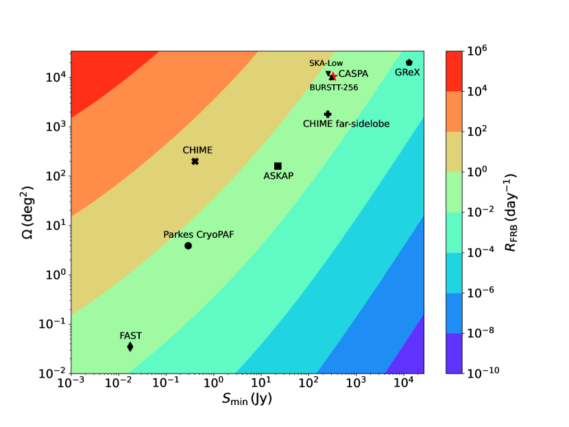
Figure 1: The detection rate contour of instruments. The x-axis represents the flux threshold in units of Jansky, the y-axis is the FoV in units of square degree, and the colour bar denotes the inferred detection number per day. The detection rate of several instruments are marked, such as the CASPA (star in red), Parkes CryoPAF (circle), GReX (pentagon), BURSTT-256 (triangle up), SKA-Low (triangle down), CHIME far-sidelobe (plus), CHIME (cross), ASKAP (square) and FAST (diamond).

3.1 The Monte Carlo Simulations

In order to obtain the properties of the detectable FRBs for a given system we use the following recipe:

1. Sample the FRB luminosities, $L$, according to the Schechter function as follow,
   

   $$\phi(L)\,\mathrm{d}L=\phi^{*}\left(\frac{L}{L^{*}}\right)^{\alpha}e^{-\frac{L}{L^{*}}}\,\mathrm{d}\left(\frac{L}{L^{*}}\right)\,,$$ (6)

   where $\phi^{*}=339_{-313}^{+1074}\,\mathrm{Gpc}^{-3}\,\mathrm{yr}^{-1}$, $\alpha=-1.79_{-0.35}^{+0.31}$ and $\log L^{*}=44.46_{-0.38}^{+0.71}$ according to Luo et al. (2020).

2. Sample the intrinsic FRB pulse widths in the local rest frame of FRBs using the log-normal distribution constrained in Luo et al. (2020):
   

   $$f_{\mathrm{w}}(\log w_{\mathrm{i}})=\frac{1}{\sqrt{2\pi\sigma_{\rm w}^{2}}}\exp\left[-\frac{(\log w_{\mathrm{i}}-\mu_{\rm w})^{2}}{2\sigma_{\rm w}^{2}}\right]\,,$$ (7)

   where the measured dimensionless mean value is $\mu_{w}=0.13_{-0.13}^{+0.11}$ and the standard deviation is $\sigma_{w}=0.33_{-0.06}^{+0.09}$ (Luo et al., 2020).

3. Consider the cosmological principle for galaxy distribution and possible cosmological evolution for FRB population summarised in Zhang et al. (2021), by sampling the FRB redshifts, $z$. The redshift distribution is given as

   $$f_{z}(z) =\frac{\mathrm{d}N}{\mathrm{d}t\mathrm{d}V}\frac{\mathrm{d}t}{\mathrm{d}t_{\mathrm{obs}}}\frac{\mathrm{d}V}{\mathrm{d}z}$$ (8)

   $$=\left[(1+z)^{a\eta}+\left(\frac{1+z}{B}\right)^{b\eta}+\left(\frac{1+z}{C}\right)^{c\eta}\right]^{1/\eta}$$

   $$\quad\frac{1}{1+z}\cdot\frac{c\,D_{c}^{2}(z)}{H_{0}E(z)}\,,$$

   where $a=3.4$, $b=-0.3$, $c=-3.5$, $B\simeq 5000$, $C\simeq 9$ and $\eta=-10$ according to Zhang et al. (2021). We then calculate the DM values corresponding to the contribution from the intergalactic medium (IGM) at the sampled redshifts.

4. Use the DM distributions of host galaxies at redshift bin $z$ described by Luo et al. (2018) to sample the DM values contributed by host galaxies in the local rest frame of the sources. We assume that the DM distribution of host galaxies in the nearby Universe is given as a logarithmic double Gaussian function.

   $$f_{\mathrm{host}}(\mathrm{DM}_{\rm host}|z=0)=$$ (9)

   $$\sum_{i=1}^{2}a_{i}\exp\left\{-\left[\frac{\log(\mathrm{DM}_{\rm host}|z=0)-b_{i}}{c_{i}}\right]^{2}\right\}\,,$$

   where $a_{1}=0.0049$, $b_{1}=0.8665$, $c_{1}=1.009$, $a_{2}=0.0126$, $b_{2}=1.069$, $c_{2}=0.5069$ as given for the galaxy case of ALGs(NE2001) in Luo et al. (2018).

5. Sample the DM values caused locally by the FRB progenitors using the uniform distribution from 0 to 50 $\mathrm{pc}\,\mathrm{cm}^{-3}$, as assumed in Luo et al. (2018).

6. Produce Galactic DM values using the YMW16 model (Yao et al., 2017), and then sum the DMs from all of components mentioned above to obtain the total observed values.

7. Obtain the beam responses by generating a random uniform distribution of FRB positions. For the fixed horizontal arrays we add a factor of $\cos{\theta}$ to compensate for the change of effective collecting area with zenith angle, $\theta$. For the CHIME far-sidelobe monitor, the beam shape is modelled using the results from Amiri et al. (2022).

8. Compute the received peak flux density using the simulated luminosities, redshifts, and the beam responses of FRB positions within the beam size. Note that we assume a flat spectrum of FRBs (spectral index as 0) here.

9. Based on the intrinsic pulse widths, redshifts and DMs of FRBs obtained in the steps above, calculate the observed pulse width impacted by DM smearing and scattering broadening. In particular, the DM smearing is given as

   $$\tau_{\mathrm{DM}}=8.3\mu\mathrm{s}\,\frac{\Delta f_{\mathrm{ch}}}{\mathrm{MHz}}\,\frac{\mathrm{DM}}{\mathrm{pc}\,\mathrm{cm}^{-3}}\,\left(\frac{f_{c}}{\mathrm{GHz}}\right)^{-3}\,,$$ (10)

   and we adopt the scattering-DM empirical relation from Krishnakumar et al. (2015) as follows.

   $$\tau_{\mathrm{sc}}=3.6\times 10^{-6}\,\mathrm{ms}\,\mathrm{DM}^{2.2}(1+1.94\times 10^{-3}\,\mathrm{DM}^{2.0})\,.$$ (11)

10. Select the FRBs where the peak fluxes are above the instrumental threshold. The threshold of peak flux density is calculated using the radiometer equation as below.

    $$S_{\mathrm{min}}=\frac{\rm S/N_{0}\,SEFD}{\sqrt{N_{\mathrm{pol}}\,\mathrm{BW}w}}\cdot{\rm MAX}\left(1,\sqrt{\frac{t_{\mathrm{res}}}{w}}\right)\,,$$ (12)

    where $\mathrm{S/N}_{0}$ is the threshold of signal-to-noise ratio, e.g., $\mathrm{S/N}_{0}=10$ is adopted in this paper, $\mathrm{BW}$ is the bandwidth, $N_{\mathrm{pol}}$ the number of combined polarization channels, $\mathrm{SEFD}$ is system equivalent flux density and $w$ is the observed width of the FRB. For systems with poor time resolutions, such as BURSTT and SKA-Low, the fluence threshold is converted using $t_{\mathrm{res}}$ as time resolution of the system.

11. Generate waiting times of adjacent events during blind search. particularly, the distribution of waiting times follows the Poisson process as below

    $$f_{\mathrm{t}}(\Delta t)=\lambda e^{-\lambda\Delta t}.$$ (13)

    The expected number of events is given as $\lambda=\rho\Omega t$, where $\Omega$ is the FoV in units of deg² and $t$ is the observing time. The mean event rate $\rho$ is calculated by integrating the luminosity function in units of volumetric rate along redshift bins, that is,

    $$\rho=\int_{0}^{\infty}\frac{1}{1+z}\frac{D(z)^{2}}{H(z)}\mathrm{d}z\int_{\log L_{\mathrm{min}}}^{\infty}\phi(\log L)\,\mathrm{d}\log L\,.$$ (14)

    Note that

    $$L_{\mathrm{min}}(S_{\mathrm{min}},z)=4\pi D_{\rm L}^{2}(z)\Delta\nu_{0}S_{\mathrm{min}}\,,$$ (15)

    where the threshold of flux density $S_{\mathrm{min}}$ is described in Step (x). Note that this does not consider any frequency dependence under the assumption of a flat spectrum for FRBs, thus no k-correction is needed in this case.

3.2 Detection rate distributions

We simulate 100,000 FRBs following this Monte Carlo recipe above and then obtain the detection rate densities of multiple instruments in DM space, which are shown in Figure 2. Note that the event rate density of the DM distribution is calculated using

$$\mathcal{R}_{\mathrm{DM}}=P(\mathrm{DM})\cdot\frac{N_{\mathrm{f}}}{t_{\mathrm{obs}}}\,,$$ (16)

where $P(\mathrm{DM})$ is the probability density of DM distribution function, given by $\int P(\mathrm{DM})\mathrm{d}\,\mathrm{DM}=1$. $N_{\mathrm{f}}$ and $t_{\mathrm{obs}}$ are the total number of simulated FRBs and total observing time in the simulations, respectively. The expected average detection rate of specific instrument in Table 1 is obtained by integrating the curves in Figure 2.

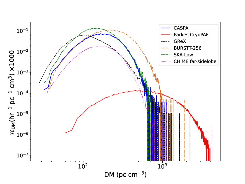
Figure 2: DM distributions of simulated FRB detected by several instruments. The x-axis is the total DM in units of $\mathrm{pc}\,\mathrm{cm}^{-3}$, the y-axis denotes the event rate density in units of per hour per unit of DM.

The peak detection rate for each instrument reflects the integrated detection rate directly. For instance, the SKA-Low and BURST-256 systems have the highest event rate densities. Although the DM distributions of different instruments are impacted by both FoV and sensitivity, the range of DM distribution is mostly determined by sensitivity, for instance, the DM distribution for the Parkes CryoPAF ranges from hundreds to thousands of $\mathrm{pc}\,\mathrm{cm}^{-3}$ with a peak at $800\,\mathrm{pc}\,\mathrm{cm}^{-3}$, which is consistent with previous Parkes detections (Arcus et al., 2022). By contrast, for all-sky monitors such as the ground-based phased array or a dipole array, the detectable FRBs are more likely to be low-DM. As highlighted by Figure 2, the Parkes CryoPAF and our proposed ground-based all-sky monitor will be complementary in terms of the very different DM distribution of the detectable FRBs.

4 Localization

The FRBs detected using the all-sky monitor will be relatively close, as shown in Figure 2. If the events can also be localised for these nearby FRBs then multi-wavelength observations of the FRB hosts and studies of the progenitor environment will be much more effective. As described in the next section, this all-sky monitor will also allow the electromagnetic follow-up (and hence localisation) of gravitational wave events. We consider some localisation options below.

4.1 One phased-array station

At zenith, the phased array beam will have a half power beam width (HPBW) of 7 degrees at 1.4 GHz . The position of an event within the beam can be determined from the amplitudes in adjacent beams to an accuracy of HPBW/signal to noise. A 10 sigma event will be positioned to an accuracy of 40’. This will only be sufficient to identify extremely close-by FRB hosts, but it will be more than adequate to search for coincidences with gravitational wave events.

Since the aperture is fully sampled by the proposed array there is no positional ambiguity due to multiple sidelobes. Both the position within the beam which detects the FRB and/or gravitational wave event and its fluence will be well determined for all candidates.

4.2 Three phased-array stations

To obtain higher precision we will need multiple spatially separated stations. We then have two possible procedures. We could either use intensity based pulse time of arrival (ToA) measurements or interferometric voltage cross-correlations between stations. Intensity based ToAs are what e.g. GReX is planning. For FRBs the ToA can be measured to a precision of about 0.1 msec so even with stations separated by 1000s of km this would only provide a localisation precision of about 1 degree which is no better than the single coherent station.

However wide bandwidth voltage cross correlations will be able to measure delays to better than a wavelength making sub-arcsecond precision position measurement possible with baselines of only 10s of km. These individual all sky monitor stations will have insufficient sensitivity for the normal astrometric calibration procedures using astronomical sources, so it would be necessary to tie them to an existing connected element array with a common clock. An obvious opportunity would be to locate the monitor stations with the outer antennas of the ASKAP array. While increasing the baseline length to VLBI scales allows increasing localisation precision, maintaining diffraction-limited accuracy would pose an increasing calibration challenge.

Since the transient events will be from point sources and would almost certainly be the only transient in the beam at a given time, three stations are sufficient to determine a 2D position. To simplify the processing we envisage a full FRB dispersion measure search being done on all 72 beams at one station (the primary station). This is preferably the station with the lowest RFI environment. The other two stations will have simple voltage buffers a few seconds long on each receiver port. Voltage dumps will be triggered by the primary station and the beam forming and post processing will be carried out off-line. This greatly reduces the backend cost of the two secondary stations and greatly reduces the data rate to an easily manageable level.

5 Discussion on the Science Cases

Given the large FoV, but relatively low sensitivity, the ground-based phased array would be used for different science cases than the more traditional radio facilities such as CHIME, ASKAP, Parkes, MeerKAT and FAST. Here we provide a summary of some of the likely science cases.

5.1 Uncovering FRBs in the nearby Universe

Using the detection rate distributions described in Section 3, we see how the sensitivity of a given system influences the DM range of the FRBs that will be detected. The all-sky monitors necessarily have relatively low sensitivity and hence a larger number of FRBs with low-DM in the nearby Universe are likely to be discovered.

To explore the population that CASPA would uncover in more detail, we re-analysed the simulated FRBs for CASPA and for the Parkes CryoPAF to show the Fluence versus extra Galactic DM distribution (see Figure 3). Clearly the Parkes CryoPAF will detect more high-DM FRBs, which will be used to study the FRB evolution at high redshift. In contrast, the FRBs detected by CASPA have rather low extra-Galactic $\mathrm{DM}_{\rm E}$ ranging from 50 to 300 $\mathrm{pc}\,\mathrm{cm}^{-3}$, but very high fluences from $10^{2}$ to $10^{4}$ Jy ms. At the time of writing, there have been more than 40 FRBs with confirmed host galaxies (Gordon et al., 2023) with a redshifts up to 1.01 (Ryder et al., 2023). The localised FRB samples at low-redshift ($z<0.1$) are so limited that the population of nearby FRBs is not well characterised. Hence, understanding the properties of these nearby sources is essential to bridge the energy gap between Galactic and cosmological FRBs, and it is also needed for a comprehensive view on the evolution of FRBs. Since the luminosity function that we used in these simulations is constructed from the sample of more distant FRBs, our population modelling is the most conservative case for such FRBs. Our modeling assumes a smooth volumetric FRB rate, but the star-formation rate in the local volume ($<10$ Mpc) is higher than a large comoving volume by a factor of 2 (Mattila et al., 2012), so we may expect to detect even more FRBs from our local Universe and their spatial distribution will not be uniform.

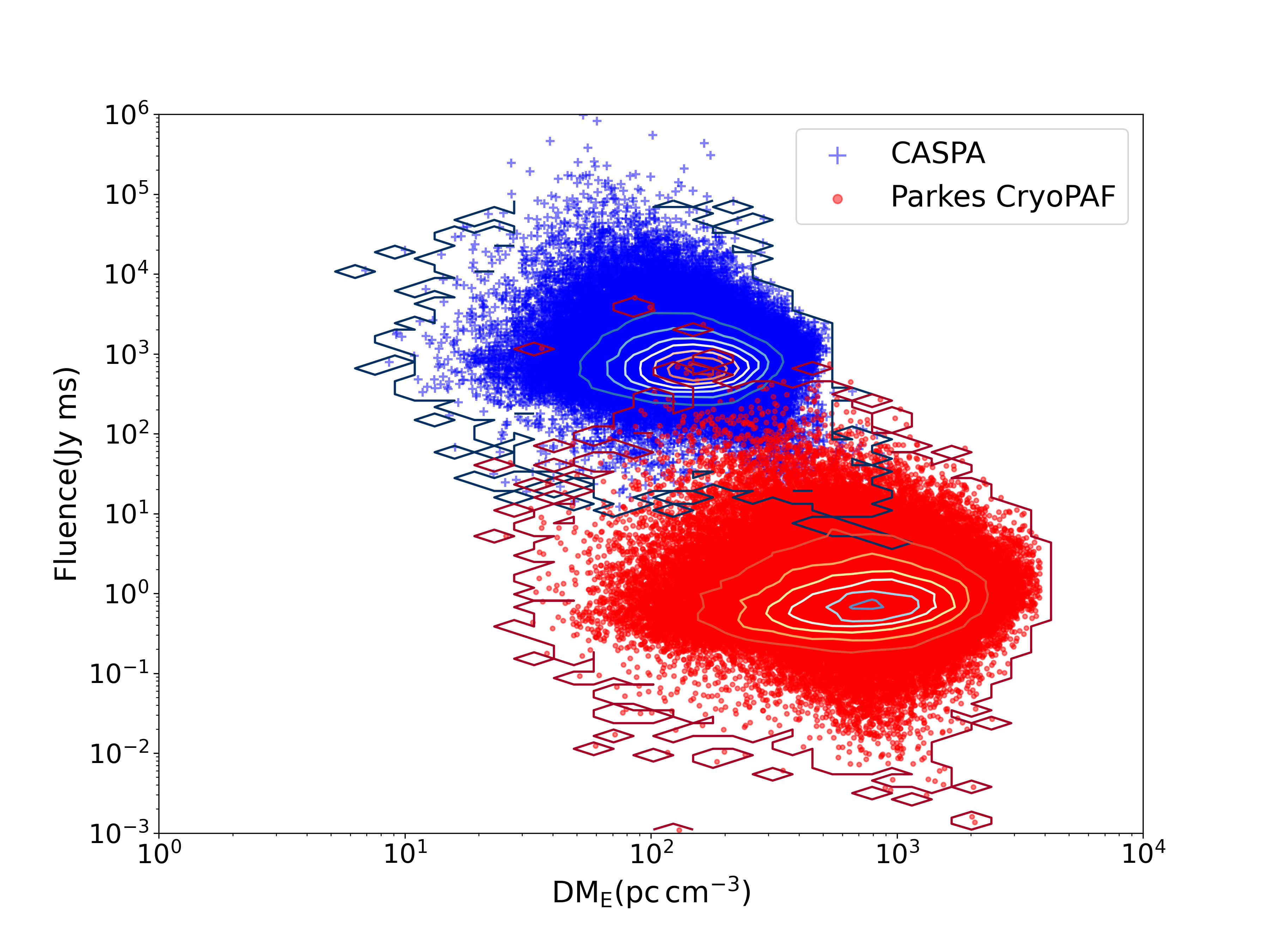
Figure 3: Fluence - $\mathrm{DM}_{\rm E}$ distribution for Parkes CryoPAF and CASPA. The x-axis represents the extragalactic DM in logarithmic scale, and the y-axis is fluence in units of Jy ms. The 100,000 simulated FRBs for CASPA are marked by blue pluses and those for Parkes CryoPAF are marked by red crosses. The number densities of these two FRB clusters are denoted by the contour lines correspondingly.

5.2 Extending the FRB luminosity function

For FRBs at larger distances, we will only be able to detect ultra-luminous FRBs. Any such ultra-luminous events must be rare requiring a large FoV monitor to find them. We compare the luminosity distributions of three different systems; CASPA, the Parkes CryoPAF and FAST (Nan et al. 2011) in Figure 4. The peak of the luminosity distribution for CASPA is close to the higher cut-off of the input luminosity function we used in the Monte Carlo simulations described in earlier. This distribution is strongly skewed to the rare highest luminosity FRBs for the less sensitive instruments so they will set the strongest constraints on the high luminosity cut-off. Some studies of the cut-off luminosity from the various FRB samples have been made, e.g., using the ASKAP localised FRBs combined with the Parkes non-localised ones (James et al., 2022) and using the first CHIME/FRB Catalogue (Shin et al., 2023). However, the intrinsic cut-off luminosity is not well determined because of selection biases that occur, especially when conducting surveys with the large telescopes. A dedicated all-sky monitor such as CASPA would be a powerful instrument to constrain the high-energy limit of the FRB emission mechanism.

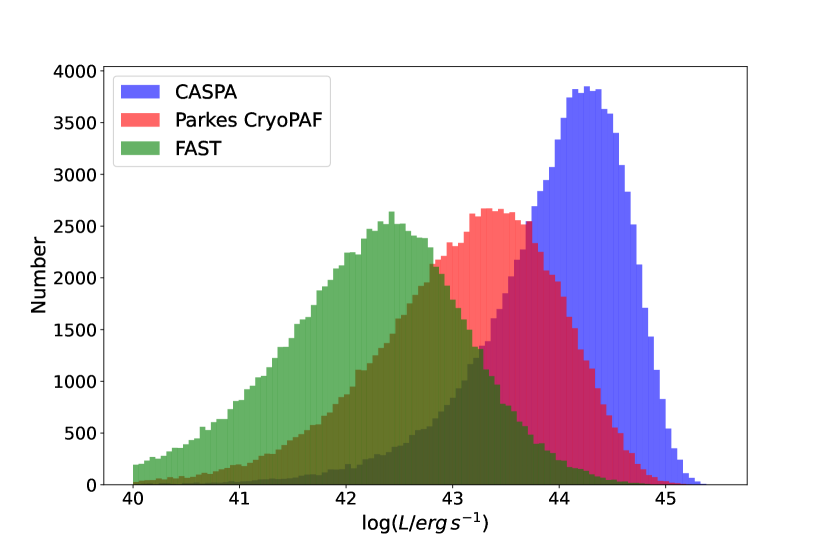
Figure 4: Luminosity distributions of the simulated FRBs that would be detected by CASPA (blue), Parkes CryoPAF (red) and FAST (green), respectively. The x-axis represents the luminosity of FRBs in logarithmic scale, the y-axis is the number of simulated FRBs detected.

5.3 Shadowing GW events

From the simulations, we can also obtain the dispersion-redshift distribution for the All-sky Phased Array, which is shown in Figure 5. The sample tells us the redshifts of FRBs that would be detected by CASPA will usually be low, peaking at $z=0.06$ with a range from 0 to 0.3.

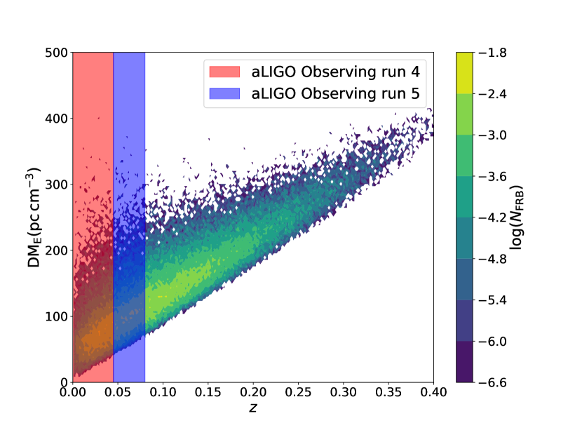
Figure 5: $z-\mathrm{DM}_{\rm E}$ distributions of simulated FRBs for CASPA. The x-axis denotes the cosmological redshifts and the y-axis denotes the extragalactic DM in units of $\mathrm{pc}\,\mathrm{cm}^{-3}$, and the colour bar is the logarithmic number density of this 2-D histogram. The shaded regions from left to right represent the redshift ranges of aLIGO O4 (red) and O5 (blue) respectively.

The large FoV allows the all-sky monitor to shadow gravitational wave detections by the advanced Laser Interferometer Gravitational-Wave Observatory (aLIGO). The All-Sky monitor bias to detections of nearby events is also an advantage. Adopting the distance limits estimated for aLIGO Observing run 4 (O4) and 5 (O5) in Abbott et al. (2020b), we have included these distance limits in Figure 5. The all-sky monitor can fully cover all the possible FRB-GW association events. There are some theoretical models that account for FRBs as being double neutron star mergers (Totani, 2013; Yamasaki et al., 2018). In such a scenario, we would expect to observe possible FRB-GW associated events by both radio telescopes and GW detectors.

Radio counterparts associated with gravitational wave (GW) events involving at least one neutron star or white dwarf have been predicted well before the discovery of FRBs (e.g. Hansen & Lyutikov, 2001), and scenarios have been proposed to produce emission during the inspiral phase, at point of merger, from the post-merger remnant, and/or from the remnant’s subsequent collapse (for reviews, see Chu et al., 2016; Rowlinson & Anderson, 2019). However, the sensitivity limit of the current gravitational wave detector network to such mergers is less than 200 Mpc (The LIGO Scientific Collaboration et al., 2021), meaning that if such events are associated with the known population of FRBs (as suggested by Moroianu et al. 2023), their GW signatures will be undetectable.

This suggests that the optimum way to search for radio emission associated with GW events is “shadowing” — constantly monitoring the same sky viewed by the LIGO–VIRGO–KARGA (LVK) network. Our proposed system will be ideal for such a purpose, and we expect to have time-coincident radio data for a large fraction of all GW detections. The large positional errors characteristic of GW detections will be readily covered by the large FoV of this ground-based array. Furthermore, there will be no need to re-point upon receiving a trigger: the instrument will continue to monitor the visible part of the GW localisation region as it passes overhead. This will help overcome cases where public alert information is delayed, as was the case for GW 190425 (Abbott et al., 2020a).

If a fraction of the observed FRB population does originate from compact object mergers, their fluence at Earth, if emitted from within the LVK horizon, would be readily detectable by our proposed system according to Figure 5. However, FRB-like emission may have difficulty escaping the merger ejecta (Bhardwaj et al., 2023). In such a scenario, any visible bursts must be produced either pre-merger, or be delayed by perhaps years post-merger. It is impossible for targeted follow-up programs to be sensitive to either scenario (James et al., 2019; Dobie et al., 2019); only an all-sky monitor therefore stands a chance of detecting such radio bursts.

5.4 Monitoring magnetar flares and burst storms

Giant flares from Galactic (and possibly extra-galactic) magnetars have been observed at X-ray and gamma-ray wavelengths (Hurley et al., 1999, 2005; Svinkin et al., 2021). The short duration (milliseconds to seconds) of the prompt emission from these events, combined with their low event rate makes conducting contemporaneous radio observations extremely difficult with the limited FoV of traditional telescopes. Non-detections of a coincident radio burst from the 2004 giant flare of SGR 1806$-$20 in the far sidelobe of the Parkes Multibeam set a fluence upper-limit of 1.1-110 MJy ms, depending on the assumed attenuation factor (Tendulkar et al., 2016). More recently CHIME/FRB reported no detections of a burst coincident with GRB 231115A, suggested to be a giant flare from a magnetar located in M82, down to a limiting fluence of 720 Jy ms (Curtin & CHIME/FRB Collaboration, 2023). There has however been some success in performing follow-up observations of magnetars undergoing ‘burst storms’ events where hundreds to thousands of hard X-ray bursts are emitted over the course of a few days. Both the April 2020 FRB-like burst and more recent intermediate intensity radio bursts from SGR 1935$+$2154 have been associated with bright X-ray bursts that were emitted during such burst storms (Giri et al., 2023). This proposed all sky monitor may provide similar radio detections as was the case for the enormously energetic FRB-like burst from magnetar SGR 1935$+$2154 (CHIME/FRB Collaboration et al., 2020; Bochenek et al., 2020). Notably, this flare was only 40 times less energetic than the weakest extragalactic FRB known at the time. If a significant fraction of the extragalactic FRB population follows the same emission mechanism that was involved in the SGR 1935$+$2154, then finding additional events in our galaxy will provide invaluable clues about the progenitors and the emission mechanism of FRBs.

An all-sky monitor situated in the Southern Hemisphere will, for the first time, continuously monitor the entire Southern galactic plane and Magellanic Clouds. This would allow for the Galactic event rate and energy distribution to be determined for Galactic magnetars going two orders of magnitude fainter than SGR 1935+2154.

5.5 Finding the unknown

Historically, astronomical serendipitous discoveries have always followed any extension of the observing parameter space (Kellerman & Bouton, 2023). With unprecedented FoV, CASPA will have the potential to explore a large parameter space which has not been accessible before and hence would have the potential to find something totally unknown . In recent years, anomalous detections have been reported by the Australian Square Kilometre Array Pathfinder (ASKAP) widefield surveys, e.g., the Odd Radio Circles (ORCs, Norris et al. 2021) from the Evolutionary Map of the Universe Pilot Survey (EMU) and a weird polarized radio source (Wang et al., 2021) from the Variables and Slow Transients (VAST).

All sky monitors are only practical for arrays with small diameter and low angular resolution. Such arrays are completely confusion limited but short period transients such as FRBs are easily detectable as signal differences on time scales short compared to the motion of the sky through the fixed pattern of beams. Hence the primary science case described in this paper is to detect FRBs. However, we may be able to extend this to longer-duration and longer-period transient sources by taking advantage of the fixed pattern of beams and the low angular resolution. The sky will move through the 15 deg beams at the survey frequency in an hour so we could extend the search for transients to much longer time scales. Any strong rare events with time scales similar such as those due to the long duration transients discovered by the Murchison Widefield Array (Hurley-Walker et al., 2022, 2023) would be detectable. We could even form a reference baseline as the sky moves through the beams to extend the detection of any unexpected changes to even longer time scales. The detectability of a range of short-duration events has been modelled by Luo et al. 2022 and Yong et al. 2022).

6 Summary and Outlook

Large FoV instruments can play a critical role in the blind search both for rare and for nearby FRBs, but it is physically difficult to combine a large FoV with the large apertures needed for high sensitivity. One solution is a compact phased array on the ground looking up and forming enough independent beams from the coherent combination of all elements to provide the large FoV while maintaining the sensitivity of the total aperture. We have argued that the optimum configuration for an all-sky monitor is a close packed array with element separation $d=\lambda/2$. We described such a phased array with 72 active receiver elements working in the frequency range of 0.7-1.4 GHz. This will have a fully sampled extremely large instantaneous FoV of $\sim 10^{4}$ square degrees. By coherently combining all elements, the sensitivity in each of the 72 beams is the same as having a 3 m² aperture with no additional image processing required. As technology improves, arrays with thousands, or even tens of thousands of elements, corresponding to apertures up to 20-m diameter will become possible. The FRB dispersion measure search still has to be done at the full 700 MHz bandwidth in each of the 72 dual polarization beams, hence it is important to minimise the computational requirements without compromising either the dispersion measure search range or the sampling time. We have included an analysis of a representative array configuration, CASPA, which maximises sky coverage with the minimum number of independent signal paths to process. We do not explore design details any further in this paper but the beam forming and processing systems for CASPA have already been developed for the Parkes CryoPAF.

If a similar system is deployed in the Northern Hemisphere, 24 hour observations will cover the entire sky every day, and may detect 4 or 5 FRBs per week. These all-sky monitors will be optimal for detecting bright FRBs in the nearby Universe and for constraining the high end of the FRB luminosity function. The use of three monitors would allow sub arc-second level localisation of the FRB events allowing multiwavelength follow-up. The unprecedented instantaneous FoV at radio wavelengths opens up a very large parameter space for serendipitous discoveries of the unknown, including short duration techno-signatures. See chapter 6 discussing the Omni-directional SETI Search in Ekers et al. (2002) and Sokolowski et al. (2022).

R.L. is supported by the National Natural Science Foundation of China (Grant No. 12303042). C.W.J. acknowledges support by the Australian Government through the Australian Research Council’s Discovery Projects funding scheme (project DP210102103).

References

- Abbott et al. (2020a) Abbott, B. P., Abbott, R., Abbott, T. D., et al. 2020a, ApJ, 892, L3
- Abbott et al. (2020b) —. 2020b, Living Reviews in Relativity, 23, 3
- Amiri et al. (2022) Amiri, M., Bandura, K., Boskovic, A., et al. 2022, ApJ, 932, 100
- Arcus et al. (2022) Arcus, W. R., James, C. W., Ekers, R. D., & Wayth, R. B. 2022, MNRAS, 512, 2093
- Bhandari et al. (2022) Bhandari, S., Heintz, K. E., Aggarwal, K., et al. 2022, AJ, 163, 69
- Bhardwaj et al. (2023) Bhardwaj, M., Palmese, A., Magaña Hernandez, I., D’Emilio, V., & Morisaki, S. 2023, arXiv e-prints, arXiv:2306.00948
- Bochenek et al. (2020) Bochenek, C. D., Ravi, V., Belov, K. V., et al. 2020, Nature, 587, 59
- CHIME/FRB Collaboration et al. (2020) CHIME/FRB Collaboration, Andersen, B. C., Bandura, K. M., et al. 2020, Nature, 587, 54
- CHIME/FRB Collaboration et al. (2021) CHIME/FRB Collaboration, Amiri, M., Andersen, B. C., et al. 2021, ApJS, 257, 59
- Chu et al. (2016) Chu, Q., Howell, E. J., Rowlinson, A., et al. 2016, MNRAS, 459, 121
- Connor et al. (2021) Connor, L., Shila, K. A., Kulkarni, S. R., et al. 2021, PASP, 133, 075001
- Cordes (2007) Cordes, J. M. 2007, in American Astronomical Society Meeting Abstracts, Vol. 211, American Astronomical Society Meeting Abstracts, 146.04
- Cordes & Chatterjee (2019) Cordes, J. M., & Chatterjee, S. 2019, ARA&A, 57, 417
- Curtin & CHIME/FRB Collaboration (2023) Curtin, A. P., & CHIME/FRB Collaboration. 2023, The Astronomer’s Telegram, 16341, 1
- Dixon (1995) Dixon, R. S. 1995, Acta Astronautica, 35, 745
- Dobie et al. (2019) Dobie, D., Murphy, T., Kaplan, D. L., et al. 2019, PASA, 36, e019
- Dunning et al. (2023) Dunning, A., Barker, S., Carter, N., et al. 2023, in 2023 IEEE International Symposium on Antennas and Propagation and USNC-URSI Radio Science Meeting (USNC-URSI), 757–758
- Ekers et al. (2002) Ekers, R. D., Culler, K., Billingham, J., & Scheffer, L. 2002, SETI 2020 : a roadmap for the search for extraterrestrial intelligence / produced for the SETI Institute by the SETI Science & Technology Working Group
- Giri et al. (2023) Giri, U., Andersen, B. C., Chawla, P., et al. 2023, arXiv e-prints, arXiv:2310.16932
- Gordon et al. (2023) Gordon, A. C., Fong, W.-f., Kilpatrick, C. D., et al. 2023, ApJ, 954, 80
- Hansen & Lyutikov (2001) Hansen, B. M. S., & Lyutikov, M. 2001, MNRAS, 322, 695
- Hotan et al. (2021) Hotan, A. W., Bunton, J. D., Chippendale, A. P., et al. 2021, PASA, 38, e009
- Hurley et al. (1999) Hurley, K., Cline, T., Mazets, E., et al. 1999, Nature, 397, 41
- Hurley et al. (2005) Hurley, K., Boggs, S. E., Smith, D. M., et al. 2005, Nature, 434, 1098
- Hurley-Walker et al. (2022) Hurley-Walker, N., Zhang, X., Bahramian, A., et al. 2022, Nature, 601, 526
- Hurley-Walker et al. (2023) Hurley-Walker, N., Rea, N., McSweeney, S. J., et al. 2023, Nature, 619, 487
- James et al. (2019) James, C. W., Anderson, G. E., Wen, L., et al. 2019, MNRAS, 489, L75
- James et al. (2022) James, C. W., Prochaska, J. X., Macquart, J. P., et al. 2022, MNRAS, 509, 4775
- Kellerman & Bouton (2023) Kellerman, K. I., & Bouton, E. N. 2023, Star Noise: Discovering the Radio Universe, doi:10.1017/9781009023443.019
- Kirsten et al. (2022) Kirsten, F., Marcote, B., Nimmo, K., et al. 2022, Nature, 602, 585
- Krishnakumar et al. (2015) Krishnakumar, M. A., Mitra, D., Naidu, A., Joshi, B. C., & Manoharan, P. K. 2015, ApJ, 804, 23
- Lin et al. (2022) Lin, H.-H., Lin, K.-y., Li, C.-T., et al. 2022, PASP, 134, 094106
- Lin et al. (2023) Lin, H.-H., Scholz, P., Ng, C., et al. 2023, arXiv e-prints, arXiv:2307.05261
- Lorimer et al. (2007) Lorimer, D. R., Bailes, M., McLaughlin, M. A., Narkevic, D. J., & Crawford, F. 2007, Science, 318, 777
- Luo et al. (2018) Luo, R., Lee, K., Lorimer, D. R., & Zhang, B. 2018, MNRAS, 481, 2320
- Luo et al. (2020) Luo, R., Men, Y., Lee, K., et al. 2020, MNRAS, 494, 665
- Luo et al. (2022) Luo, R., Hobbs, G., Yong, S. Y., et al. 2022, MNRAS, 513, 5881
- Marcote et al. (2017) Marcote, B., Paragi, Z., Hessels, J. W. T., et al. 2017, ApJ, 834, L8
- Mattila et al. (2012) Mattila, S., Dahlen, T., Efstathiou, A., et al. 2012, ApJ, 756, 111
- Moroianu et al. (2023) Moroianu, A., Wen, L., James, C. W., et al. 2023, Nature Astronomy, 7, 579
- Nan et al. (2011) Nan, R., Li, D., Jin, C., et al. 2011, International Journal of Modern Physics D, 20, 989
- Niu et al. (2022) Niu, C. H., Aggarwal, K., Li, D., et al. 2022, Nature, 606, 873
- Norris et al. (2021) Norris, R. P., Intema, H. T., Kapińska, A. D., et al. 2021, PASA, 38, e003
- Petroff et al. (2019) Petroff, E., Hessels, J. W. T., & Lorimer, D. R. 2019, A&A Rev., 27, 4
- Petroff et al. (2022) —. 2022, A&A Rev., 30, 2
- Rowlinson & Anderson (2019) Rowlinson, A., & Anderson, G. E. 2019, MNRAS, 489, 3316
- Ryder et al. (2023) Ryder, S. D., Bannister, K. W., Bhandari, S., et al. 2023, Science, 382, 294
- Shin et al. (2023) Shin, K., Masui, K. W., Bhardwaj, M., et al. 2023, ApJ, 944, 105
- Sokolowski et al. (2022) Sokolowski, M., Price, D. C., & Wayth, Randall, B. 2022, in 2022 3rd URSI Atlantic and Asia Pacific Radio Science Meeting (AT-AP-RASC, 1
- Sokolowski et al. (2021) Sokolowski, M., Wayth, R. B., Bhat, N. D. R., et al. 2021, PASA, 38, e023
- Staveley-Smith et al. (1996) Staveley-Smith, L., Wilson, W. E., Bird, T. S., et al. 1996, PASA, 13, 243
- Svinkin et al. (2021) Svinkin, D., Frederiks, D., Hurley, K., et al. 2021, Nature, 589, 211
- Tendulkar et al. (2016) Tendulkar, S. P., Kaspi, V. M., & Patel, C. 2016, ApJ, 827, 59
- The LIGO Scientific Collaboration et al. (2021) The LIGO Scientific Collaboration, the Virgo Collaboration, the KAGRA Collaboration, et al. 2021, arXiv e-prints, arXiv:2111.03606
- Thornton et al. (2013) Thornton, D., Stappers, B., Bailes, M., et al. 2013, Science, 341, 53
- Totani (2013) Totani, T. 2013, PASJ, 65, L12
- Wang et al. (2021) Wang, Z., Kaplan, D. L., Murphy, T., et al. 2021, ApJ, 920, 45
- Yamasaki et al. (2018) Yamasaki, S., Totani, T., & Kiuchi, K. 2018, PASJ, 70, 39
- Yao et al. (2017) Yao, J. M., Manchester, R. N., & Wang, N. 2017, ApJ, 835, 29
- Yong et al. (2022) Yong, S. Y., Hobbs, G., Huynh, M. T., et al. 2022, MNRAS, 516, 5832
- Zhang et al. (2021) Zhang, R. C., Zhang, B., Li, Y., & Lorimer, D. R. 2021, MNRAS, 501, 157