Compressed Online Learning of Conditional Mean Embedding

Abstract

The conditional mean embedding (CME) encodes conditional probability distributions within the reproducing kernel Hilbert spaces (RKHS). The CME plays a key role in several well-known machine learning tasks such as reinforcement learning, analysis of dynamical systems, etc. We present an algorithm to learn the CME incrementally from data via an operator-valued stochastic gradient descent. As is well-known, function learning in RKHS suffers from scalability challenges from large data. We utilize a compression mechanism to counter the scalability challenge. The core contribution of this paper is a finite-sample performance guarantee on the last iterate of the online compressed operator learning algorithm with fast-mixing Markovian samples, when the target CME may not be contained in the hypothesis space. We illustrate the efficacy of our algorithm by applying it to the analysis of an example dynamical system.

1 Introduction

Markovian stochastic kernels can be studied through their actions on reproducing kernel Hilbert space (RKHS) through the conditional mean embedding (CME). Computing expectations of distributions typically involve high-dimensional integrations. The CME reduces this problem to lightweight dimension-free inner product calculations. Such a non-parametric computational framework avoids subscriptions to specific parametric descriptions of functions and probability distributions, and has found applications in reinforcement learning [Grunewalder et al. (2012), Lever et al. (2016)], analysis of nonlinear dynamical systems [Klus et al. (2020), Kostic et al. (2022), Hou et al. (2021), Hou et al. (2023b)], and causal inference problems [Mitrovic et al. (2018), Muandet et al. (2021)], among others.

The CME $\mu$ has been defined in two ways in the literature. The first approach in [Song et al. (2009)] utilizes a composition of covariance operators and requires that the RKHS be closed under the action of the corresponding stochastic kernel. The second approach in [Grünewälder et al. (2012), Park and Muandet (2020)] is measure-theoretic and defines the CME as $\mu(x)=\mathds{E}_{Y|x}[\kappa_{Y}(\cdot,Y)|X=x]$, where the right-hand side is understood as an ${\cal H}_{Y}$-valued Bochner-integral for random variables $X,Y$, where ${\cal H}_{Y}$ is an RKHS on the domain of $Y$ with the reproducing kernel $\kappa_{Y}$. This definition allows the CME to be viewed as the solution to a regression problem in vector-valued RKHS and does not require the closure assumption needed for the first approach. In this paper, we leverage the regression viewpoint from [Grünewälder et al. (2012), Li et al. (2022)] to provide last iterate performance guarantees on compressed online learning of CME with Markovian data. Our online learning with Markovian sampling is particularly useful to analyze unknown time-homogenous Markov processes, for which the CME encodes the transition dynamics [Klus et al. (2020), Kostic et al. (2022), Hou et al. (2023b)].

1.1 Our Contributions

• We devise an online algorithm that learns a compressed representation of the CME. This stands in sharp contrast to prior works in [Song et al. (2009), Grünewälder et al. (2012), Talwai et al. (2022), Li et al. (2022), Hou et al. (2023b)] that estimate compressed/uncompressed versions of the same from a fixed batch of IID samples. Processing streaming data is particularly useful in sequential decision-making settings, e.g., with changing environments such as in [Hazan and Seshadhri (2009), Dahlin et al. (2023)] or in nonlinear adaptive filtering in [Goodwin and Sin (2014)].

• Thanks to the representer theorem [Schölkopf et al. (2001), Carmeli et al. (2010)], the solution of a regularized regression problem in RKHS can be represented as linear expansions in terms of kernel functions centered at samples. Such representations, however, become burdensome with growth in the size of the input dataset as in [Kivinen et al. (2004), Rahimi and Recht (2007), Rudi et al. (2015), Koppel et al. (2019), Hou et al. (2023a)]. To enable scaling to large data sets, we generalize a variant of the compression scheme in [Koppel et al. (2019)] from the real-valued case to vector-valued CME estimation, which combats the growth of the complexity of the learned representation.

• As opposed to the operator-theoretic viewpoint in [Grünewälder et al. (2012)] that requires the target CME to be a part of a suitably-defined vector-valued RKHS, we tackle the so-called hard learning setting from [Li et al. (2022)] with batch processing of data where that assumption is invalid, but merge it with the online sparsification technique of [Koppel et al. (2019)].

• We adopt the Lypanuov-based argument described in [Srikant and Ying (2019), Chen et al. (2022)] to study last-iterate convergence guarantees with Markovian sampling. Compared to these papers, we innovate in two ways: (1) we extend their work from Euclidean spaces to the space of Hilbert-Schmidt operators. (2) We handle a compounding bias that arises from compression of the operator representation in each iteration by carefully controlling the step-sizes.

2 RKHS Preliminaries

2.1 Real-valued RKHS

We start by formally defining a real-valued RKHS (see Berlinet and Thomas-Agnan (2011)). A separable Hilbert space on $\mathbb{X}$ with its inner product $\left({\cal H}_{X},\left\langle\cdot,\cdot\right\rangle_{{\cal H}_{X}}\right)$ of functions $f:\mathbb{X}\to\mathbb{R}$ is an RKHS, if the evaluation functional defined by $\delta_{x}f=f(x)$ is bounded (continuous) for all $x\in\mathbb{X}$. The Riesz representation theorem implies that for all $f\in{\cal H}_{X}$, there exists an element $\phi(x)\in{\cal H}_{X}$ such that $\delta_{x}f=\left\langle f,\phi(x)\right\rangle_{{\cal H}_{X}}$. Define $\kappa_{X}:\mathbb{X}\times\mathbb{X}\rightarrow\mathbb{R}$ by $\kappa_{X}(x,x^{\prime}):=\left\langle\phi\left(x\right),\phi\left(x^{\prime}\right)\right\rangle$. Then, $\kappa_{X}$ is a positive definite kernel that satisfies $\kappa_{X}(\cdot,x)\in{\cal H}_{X}$, and $\left\langle f,\kappa_{X}(\cdot,x)\right\rangle_{{\cal H}_{X}}=f(x)$, $\forall x\in\mathbb{X}$, $\forall h\in{\cal H}_{X}$. Such $\kappa_{X}$ is called a reproducing kernel and $\phi(x):=\kappa_{X}(\cdot,x)$ is a feature map. Throughout this paper, we assume that all RKHS in question are separable with bounded measurable kernels, and holds if $\kappa$ is a continuous kernel on an Euclidean space.

Consider two separable measurable spaces $\left(\mathbb{X},{\cal B}_{X}\right)$ and $\left(\mathbb{Y},{\cal B}_{Y}\right)$ with Borel sigma-field ${\cal B}_{X}$ and ${\cal B}_{Y}$, respectively. Let $\rho$ be a probability measure on $\mathbb{X}\times\mathbb{Y}$ with its marginal on $X$ denoted by $\rho_{X}$. Denote ${\cal L}_{2}(\rho_{X},\mathbb{R}):={\cal L}_{2}(\rho_{X})$ as the vector space of real-valued square-integrable functions with respect to $\rho_{X}$. Equip ${\cal L}_{2}(\rho_{X})$ with the norm $\left\|\cdot\right\|_{\rho}$ such that $\left\|f\right\|_{\rho}:=\left(\int_{\mathbb{X}}\left|f\left(x\right)\right|^{2}\mathrm{d}\rho_{X}\right)^{1/2}$ for any $f\in{\cal L}_{2}(\rho_{X})$. For any $f\in{\cal L}_{2}(\rho_{X})$, its $\rho_{X}$-equivalent class comprises all functions $g\in{\cal L}_{2}(\rho_{X})$ that $\rho_{X}\left(\left\{f\neq g\right\}\right)=0$. Let ${L_{2}\left(\rho_{X}\right)}:={\cal L}_{2}(\rho_{X})_{/\sim}$ be the corresponding quotient space equipped with the norm $\left\|\left[f\right]_{\sim}\right\|_{{L_{2}\left(\rho_{X}\right)}}=\left\|f\right\|_{\rho}$ for any $f\in{\cal L}_{2}(\rho_{X})$. In the sequel, we drop the sub-index $\sim$ for any $\left[f\right]_{\sim}\in{L_{2}\left(\rho_{X}\right)}$ and simply denote it by $\left[f\right]$. To investigate the relationship between RKHS ${\cal H}_{X}$ and ${L_{2}\left(\rho_{X}\right)}$, consider the inclusion map ${I_{\kappa}}:{\cal H}_{X}\to{L_{2}\left(\rho_{X}\right)}$ which maps a function $h\in{\cal H}_{X}$ to its $\rho_{X}$-equivalent class $\left[h\right]$. Our algorithm and analysis require the following assumptions.

Assumption 1

(a) $\sup\limits_{x\in\mathbb{X}}\sqrt{\kappa_{X}(x,x)}\leq\sqrt{K}<\infty$, $\sup\limits_{y\in\mathbb{Y}}\sqrt{\kappa_{Y}(y,y)}\leq\sqrt{K}<\infty$. (b) ${I_{\kappa}}:{\cal H}_{X}\to{L_{2}\left(\rho_{X}\right)}$ is continuous.

Part (a) implies $\sup_{x\in\mathbb{X}}\kappa_{X}(x,x)\leq K$. Part (b) implies that ${I_{\kappa}}$ is an embedding, denoted ${\cal H}_{X}\hookrightarrow{L_{2}\left(\rho_{X}\right)}$. Define $\left[{\cal H}_{X}\right]:=\left\{\left[f\right]\in{L_{2}\left(\rho_{X}\right)}:f\in{\cal H}_{X}\right\}$. Parts (a), (b) imply that ${I_{\kappa}}$ is compact.

2.2 Vector-valued RKHS and Tensor Product Hilbert Space

Let ${\cal H}_{Y}$ be a real-valued Hilbert space and ${\cal L}({\cal H}_{Y})$ be the Banach space of bounded operators from ${\cal H}_{Y}$ to itself. A ${\cal H}_{Y}$-valued Hilbert space $\left({\cal H}_{V},\left\langle\cdot,\cdot\right\rangle_{{\cal H}_{V}}\right)$ of functions $v:\mathbb{X}\to{\cal H}_{Y}$ is an ${\cal H}_{Y}$-valued RKHS if for each $x\in\mathbb{X}$, $y\in{\cal H}_{Y}$, the linear functional $v\mapsto\left\langle y,v\left(x\right)\right\rangle_{{\cal H}_{Y}}$ is bounded. ${\cal H}_{V}$ admits an operator-valued reproducing kernel of positive type $\Gamma:\mathbb{X}\times\mathbb{X}\to{\cal L}({\cal H}_{Y})$ which satisfies $\left\langle v\left(x\right),y\right\rangle_{{\cal H}_{Y}}=\left\langle v,\Gamma(\cdot,x)y\right\rangle_{{\cal H}_{V}}$ and $\left\langle y,\Gamma(x,x^{\prime})y^{\prime}\right\rangle_{{\cal H}_{Y}}=\left\langle\Gamma(\cdot,x)y,\Gamma(\cdot,x^{\prime})y^{\prime}\right\rangle_{{\cal H}_{V}}$ for all $x,x^{\prime}\in\mathbb{X}$, $y,y\in{\cal H}_{Y}$ and $v\in{\cal H}_{V}$ . Throughout this paper, we restrict our attention to the vector-valued RKHS associated with the operator-valued kernel $\kappa_{X}\left(x,x^{\prime}\right){\textrm{Id}}_{Y}$ where ${\textrm{Id}}_{Y}$ is the identity map on ${\cal H}_{Y}$ and denote it by ${\cal H}_{V}$.

Consider two separable real-valued Hilbert spaces ${\cal H}_{X},{\cal H}_{Y}$ on separable measurable spaces $\mathbb{X}$ and $\mathbb{Y}$. A bounded linear operator $A$ is a Hilbert-Schmidt (HS) operator from ${\cal H}_{X}$ to ${\cal H}_{Y}$ if $\sum_{i\in\mathbb{N}}\left\|Ae_{i}\right\|_{{\cal H}_{Y}}^{2}<\infty$ with $\{e_{i}\}_{i\in\mathbb{N}}$ an orthonormal basis (ONB) of ${\cal H}_{X}$. The quantity $\left\|A\right\|_{{\textrm{HS}}}=\left(\sum_{i\in\mathbb{N}}\left\|Ae_{i}\right\|_{{\cal H}_{Y}}^{2}\right)^{1/2}$ is the Hilbert-Schmidt norm of $A$ and is independent of the choice of ONB. We denote ${\textrm{HS}}({\cal H}_{X},{\cal H}_{Y})$ as the Hilbert space of HS operators from ${\cal H}_{X}$ to ${\cal H}_{Y}$, endowed with the norm $\left\|\cdot\right\|_{\textrm{HS}}$. See Appendix A for a detailed introduction to HS operators. For $f_{1}\in{\cal H}_{X}$ and $f_{2}\in{\cal H}_{Y}$, the tensor product $f_{1}\otimes f_{2}$ is defined as a rank-one operator from ${\cal H}_{Y}$ to ${\cal H}_{X}$,

$$\left(f_{1}\otimes f_{2}\right)g\mapsto\left\langle g,f_{2}\right\rangle_{{\cal H}_{Y}}f_{1},\quad\forall g\in{\cal H}_{Y}.$$ (1)

This rank-one operator is Hilbert-Schmidt. Given a second operator $f^{\prime}_{1}\otimes f^{\prime}_{2}$ for $f^{\prime}_{1}\in{\cal H}_{X}$, $f^{\prime}_{2}\in{\cal H}_{Y}$, their inner product is $\left\langle f_{1}\otimes f_{2},f^{\prime}_{1}\otimes f^{\prime}_{2}\right\rangle_{{\textrm{HS}}}=\left\langle f_{1},f^{\prime}_{1}\right\rangle_{{\cal H}_{X}}\left\langle f_{2},f^{\prime}_{2}\right\rangle_{{\cal H}_{Y}}$. Denote by ${\cal H}_{X}\otimes{\cal H}_{Y}$, the tensor product of two Hilbert spaces ${\cal H}_{X}$ and ${\cal H}_{Y}$ which is the completion of the algebraic tensor product with respect to the norm induced by the aforementioned inner product. Moreover, ${\textrm{HS}}({\cal H}_{X},{\cal H}_{Y})$ is isometrically isomorphic to ${\cal H}_{Y}\otimes{\cal H}_{X}$, per (Park and Muandet, 2020, Lemma C.1).

Let $L_{2}(\rho_{X},{\cal H}_{Y})$ be the ${\cal H}_{Y}$-valued Bochner square-integrable functions $y:x\mapsto y(x)$ with values in ${\cal H}_{Y}$ such that $\left\|y\right\|_{L_{2}(\rho_{X},{\cal H}_{Y})}=\left(\int_{\mathbb{X}}\left\|y\left(x\right)\right\|_{{\cal H}_{Y}}^{2}\mathrm{d}\rho_{X}\right)^{1/2}<\infty$. Consider a vector-valued RKHS ${\cal H}_{V}$ associated with the operator-valued kernel $\kappa_{X}\left(x,x^{\prime}\right){\textrm{Id}}_{Y}$, where $\kappa_{X}$ is a real-valued kernel function on $\mathbb{X}$ and ${\textrm{Id}}_{Y}\in{\cal L}({\cal H}_{Y})$ is the identity operator on ${\cal H}_{Y}$. Under Assumption 1, we have the lemma below whose proof is deferred to Appendix A.1.

Lemma 2.1.

Let Assumption 1 hold. Then, ${\cal H}_{V}$ and ${\cal H}_{Y}\otimes{\cal H}_{X}$ are isomorphic, i.e., ${\cal H}_{V}\cong{\cal H}_{Y}\otimes{\cal H}_{X}$. Moreover, ${\cal H}_{Y}\otimes[{\cal H}_{X}]\subseteq{\cal H}_{Y}\otimes{L_{2}\left(\rho_{X}\right)}\cong L_{2}(\rho_{X},{\cal H}_{Y})$.

Denote the isomorphism $\iota:L_{2}(\rho_{X},{\cal H}_{Y})\to{\cal H}_{Y}\otimes{L_{2}\left(\rho_{X}\right)}$ and $\iota_{\kappa}:{\cal H}_{Y}\otimes{\cal H}_{X}\to{\cal H}_{V}$. As we shall see in Section 3, we leverage the three pairs of isomorphism, ${\textrm{HS}}({\cal H}_{X},{\cal H}_{Y})\cong{\cal H}_{Y}\otimes{\cal H}_{X}$, $L_{2}(\rho_{X},{\cal H})\cong{\cal H}\otimes{L_{2}\left(\rho_{X}\right)}$ and ${\cal H}_{V}\cong{\cal H}_{Y}\otimes{\cal H}_{X}$, to study the CME learning problem within the space of Hilbert-Schmidt operators.

2.3 Embedding of Probability Distributions

Consider a probability space $\left(\Omega,{\cal F},\right)$ with a $\sigma$-algebra ${\cal F}$ and a probability measure . Let $X:\Omega\to\mathbb{X}$ be a random variable with distribution . Let Assumption 1 hold. The kernel mean embedding (KME) of in ${\cal H}_{X}$ is the Bochner integral ${\sf KME}_{X}:=\mathds{E}_{X}\left[\kappa_{X}(X,\cdot)\right]$, where $\mathds{E}_{X}$ is the expectation with respect to . Suppose that denotes a joint distribution over $\mathbb{X}\times\mathbb{Y}$, then can be embedded into ${\cal H}_{X}\otimes{\cal H}_{Y}$, per Berlinet and Thomas-Agnan (2011), as

$$\begin{aligned} C_{XY}:=\mathds{E}_{XY}[\phi_{X}(X)\otimes\phi_{Y}(Y)],\end{aligned}$$ (2)

where $\mathds{E}_{XY}$ is the expectation with respect to . We call $C_{XY}$ (uncentered) cross-covariance operator. Likewise, the (uncentered) covariance operator is defined as $C_{XX}=\mathds{E}_{X}[\phi_{X}(X)\otimes\phi_{X}(X)]$, which can be viewed as the embedding of the marginal distribution in ${\cal H}_{X}\otimes{\cal H}_{X}$. Let denote the conditional distribution of $Y$, given $X=x\in\mathbb{X}$. The ${\cal H}_{Y}$-valued conditional mean embedding (CME) $\mu:\mathbb{X}\to{\cal H}_{Y}$ is defined as

$$\mu(\cdot):=\mathds{E}_{Y|x}[\kappa_{Y}(\cdot,Y)|X=\cdot]\in L_{2}(\rho_{X},{\cal H}_{Y}),$$ (3)

according to Park and Muandet (2020). In addition, for all $f_{Y}\in{\cal H}_{Y}$ and $x\in\mathbb{X}$, we have $\mathds{E}_{Y|x}[f_{Y}(Y)|X=x]=\left\langle f_{Y},\mu\left(x\right)\right\rangle_{{\cal H}_{Y}}$. CME defined in Song et al. (2009) requires $C_{XX}$ to be injective and $\mathds{E}_{Y|x}[f(Y)|X=x]\in{\cal H}_{X}$ for all $f\in{\cal H}_{Y}$ and $x\in\mathbb{X}$. Under such conditions, $\mu$ admits the closed-form $\mu(x)=C_{YX}C_{XX}^{\dagger}\phi_{X}(x)$. Since our interest lies in the “hard learning” setting, we bypass such restrictive assumptions (see Klebanov et al. (2020); Park and Muandet (2020)).

3 Compressed Online Learning of the CMEs

3.1 Learning the CMEs via Nonlinear Least Squares Regression

Recall that $\rho$ is a joint distribution over $\mathbb{X}\times\mathbb{Y}$ and $\rho_{X}$ its marginal on $\mathbb{X}$. Park and Muandet (2020) considers an equivalent definition of $\mu$ in (3) as the minimizer of a least squares regression problem in the space of ${\cal H}_{Y}$-valued functions in $L_{2}(\rho_{X},{\cal H}_{Y})$ as

$$\mu_{\star}:=\mathop{\rm argmin}_{g\in L_{2}(\rho_{X},{\cal H}_{Y})}\int_{\mathbb{X}\times\mathbb{Y}}\left\|g\left(x\right)-\phi_{Y}\left(y\right)\right\|_{{\cal H}_{Y}}^{2}\mathrm{d}\rho(x,y).$$ (4)

In addition, $\mu_{\star}$ is almost surely unique per (Park and Muandet, 2020, Theorem 4.2). By the isomorphism in Lemma 2.1, for every $\mu_{\star}$, there exists a unique Hilbert-Schmidt operator $U_{\star}$ mapping from ${L_{2}\left(\rho_{X}\right)}$ to ${\cal H}_{Y}$ given by $U_{\star}=\iota^{-1}(\mu_{\star})$. In the sequel, we call $U_{\star}$ the CME operator. For well-posedness and over-fitting prevention, consider now its regularized variant over ${\cal H}_{V}$ as,

$$\mu_{\lambda}:=\mathop{\rm argmin}_{g\in{\cal H}_{V}}\frac{1}{2}\int_{\mathbb{X}\times\mathbb{Y}}\left\|g\left(x\right)-\phi_{Y}\left(y\right)\right\|_{{\cal H}_{Y}}^{2}\mathrm{d}\rho(x,y)+\frac{\lambda}{2}\left\|g\right\|_{{\cal H}_{V}}^{2}$$ (5)

with $\lambda>0$ as the regularization parameter. Again, with $\mu_{\lambda}\in{\cal H}_{V}$, associate a unique HS-operator $U_{\lambda}\in{\textrm{HS}}({\cal H}_{X},{\cal H}_{Y})$ such that

$$\mu_{\lambda}(x)=\iota_{\kappa}\left(U_{\lambda}\right)(x)=U_{\lambda}\phi_{X}(x),$$ (6)

where $\iota_{\kappa}$ is the isometric isomorphism defined in Lemma 2.1. We call this HS-operator $U_{\lambda}$ as the regularized CME operator. The isomorphism also suggests that $U_{\lambda}$ minimizes the regularized risk $R_{\lambda}:{\textrm{HS}}({\cal H}_{X},{\cal H}_{Y})\to\mathbb{R}$,

$$R_{\lambda}(U):=\frac{1}{2}\mathds{E}\left[\left\|\phi_{Y}(y)-U\phi_{X}(x)\right\|_{{\cal H}_{Y}}^{2}\right]+\frac{\lambda}{2}\left\|U\right\|^{2}_{{\textrm{HS}}({\cal H}_{X},{\cal H}_{Y})},$$ (7)

over ${\textrm{HS}}({\cal H}_{X},{\cal H}_{Y})$. We aim to solve (7) incrementally and then recover $\mu$ via (6). Key to our incremental learning paradigm is the gradient $\nabla_{U}R_{\lambda}\left(U\right)$ for $U\in{\textrm{HS}}({\cal H}_{X},{\cal H}_{Y})$ that we characterize in the next result; the proof is in Appendix B.1.

Lemma 3.1.

$\nabla R_{\lambda}(U)=UC_{XX}-C_{YX}+\lambda U\in{\textrm{HS}}({\cal H}_{X},{\cal H}_{Y})$ for any $U\in{\textrm{HS}}({\cal H}_{X},{\cal H}_{Y})$.

Setting $\nabla R_{\lambda}(U)$ equal to $0$ yields $-\lambda U=UC_{XX}-C_{YX}$. It admits the solution $U_{\lambda}=C_{YX}(C_{XX}+\lambda{\textrm{Id}})^{-1}$ which is the definition of the regularized CME in Song et al. (2009), provided it belongs to ${\textrm{HS}}({\cal H}_{X},{\cal H}_{Y})$. We now study an online algorithm that solves (7) incrementally.

3.2 Online Learning of the CME Operator

Let ${\cal D}_{t}:=\left\{\left(x_{i},y_{i}\right)\right\}_{i=1}^{t}$ be a collection of $t$ samples where $(x_{i},y_{i})\in\mathbb{X}\times\mathbb{Y}$ for $i=1,\ldots,t$. The empirical estimation of $U_{\lambda}$ is given by $U_{\lambda,\text{emp}}=C_{YX,\text{emp}}\left(C_{XX,\text{emp}}+\lambda{\textrm{Id}}\right)^{-1}$, per Hou et al. (2023a), where $C_{YX,\text{emp}}$, $C_{XX,\text{emp}}$ are the empirical estimates of the covariance operators,

$$C_{XX,\text{emp}}=\frac{1}{t}\sum_{i=1}^{t}\phi_{X}\left(x_{i}\right)\otimes\phi_{X}\left(x_{i}\right),\quad C_{YX,\text{emp}}=\frac{1}{t}\sum_{i=1}^{t}\phi_{Y}\left(y_{i}\right)\otimes\phi_{X}\left(x_{i}\right).$$ (8)

We next present our main algorithm that solves (7) incrementally using stochastic approximation. Let $\mathbb{T}=\mathbb{N}$ represent time. Let ${\cal F}=\left\{{\cal F}_{t}\right\}_{t\in\mathbb{T}}$ be a filtration where ${\cal F}_{t}$ is the $\sigma$-field generated by the history of data up to time $t$. Given a sample pair $(x_{t},y_{t})\in\mathbb{X}\times\mathbb{Y}$ for $t\in\mathbb{T}$, stochastic approximations based estimations of (cross)-covariance operators are given by

$$\widetilde{C}_{XX}(t)=\phi_{X}\left(x_{t}\right)\otimes\phi_{X}\left(x_{t}\right),\quad\widetilde{C}_{YX}(t)=\phi_{Y}\left(y_{t}\right)\otimes\phi_{X}\left(x_{t}\right).$$ (9)

Thus, an operator-valued stochastic variant of the gradient given in Lemma (3.1) is

$$\widetilde{\nabla}_{t}R_{\lambda}(x_{t},y_{t};U)=U\widetilde{C}_{XX}(t)-\widetilde{C}_{YX}(t)+\lambda U\in{\textrm{HS}}({\cal H}_{X},{\cal H}_{Y}),$$ (10)

for all $U\in{\textrm{HS}}({\cal H}_{X},{\cal H}_{Y})$ and $t\in\mathbb{T}$. Assuming $\widetilde{U}_{0}=0$, we select a step-size sequence $\left\{\eta_{t}\right\}_{t\in\mathbb{T}}\subset\mathbb{R}$, and consider the ${\cal F}_{t}$-adapted process $\left\{\widetilde{U}_{t}\right\}_{t\in\mathbb{T}}$ taking values in ${\textrm{HS}}({\cal H}_{X},{\cal H}_{Y})$,

$$\begin{aligned} \widetilde{U}_{t+1}=&\widetilde{U}_{t}-\eta_{t}\widetilde{\nabla}_{t}R_{\lambda}(x_{t},y_{t};\widetilde{U}_{t})=(1-\lambda\eta_{t})\widetilde{U}_{t}-\eta_{t}\left(\widetilde{U}_{t}\widetilde{C}_{XX}(t)-\widetilde{C}_{YX}(t)\right),\quad t\in\mathbb{T}.\end{aligned}$$ (11)

In what follows, we refer to (11) as the base operator-valued stochastic gradient descent (SGD) algorithm. Since ${\textrm{HS}}({\cal H}_{X},{\cal H}_{Y})\cong{\cal H}_{Y}\otimes{\cal H}_{X}$, we next show that (11) can be written as expansions in terms of elements in ${\cal H}_{Y}\otimes{\cal H}_{X}$. The proof is presented in Appendix D.

Lemma 3.2.

Let $\{\widetilde{U}_{t}\}_{t\in\mathbb{T}}$ be the sequence generated by (11). Let $\widetilde{\Phi}_{X,t}:=\left[\phi_{X}(x_{1}),\ldots,\phi_{X}(x_{t})\right]$ and $\widetilde{\Psi}_{Y,t}:=\left[\phi_{Y}\left(y_{1}\right),\ldots,\phi_{Y}(y_{t})\right]$. Then $\{\widetilde{U}_{t}\}_{t\in\mathbb{T}}$ admits the representation,

$$\widetilde{U}_{t+1}=\sum_{i=1}^{t}\sum_{j=1}^{t}\widetilde{W}^{ij}_{t}\left(\kappa_{Y}(y_{i},\cdot)\otimes\kappa_{X}(x_{j},\cdot)\right)=\widetilde{\Psi}_{Y,t}\widetilde{W}_{t}\widetilde{\Phi}_{X,t}^{\top},\quad\forall t\in\mathbb{T},$$ (12)

$$\widetilde{W}^{ij}_{t}=({\textrm{Id}}-\lambda\eta_{t})\widetilde{W}^{ij}_{t-1},\;\widetilde{W}^{it}_{t}=-\eta_{t}\sum_{j=1}^{t-1}\widetilde{W}^{ij}_{t-1}\kappa_{X}(x_{j},x_{t}),\;\widetilde{W}^{tt}_{t}=\eta_{t},\;t\in\mathbb{T}\setminus\{0\},\widetilde{W}_{0}=0.$$ (13)

The above result states that the iterates $\{\widetilde{U}_{t}\}_{t\in\mathbb{T}}$ generated by the base operator-valued SGD (11) can be described by a linear combination of kernel functions centered at samples seen thus far. Therefore, the implementation of (11) can be decomposed into two parts–appending the new sample to the current dictionary $\widetilde{{\cal D}}_{t}\leftarrow\widetilde{{\cal D}}_{t-1}\cup\{(x_{t},y_{t})\}$ and updating coefficients according to (13). The complexity of such an algorithm grows with the size of $\widetilde{{\cal D}}_{t}$ that accumulates at twice the rate of vector-valued RKHS interpolation due to samples $y_{i}$ and $x_{j}$. We aim to control that growth of $\widetilde{{\cal D}}_{t}$ by judiciously admitting a new sample only when the new sample brings sufficiently “new” information.

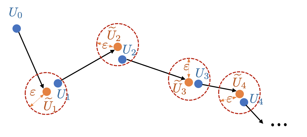
Figure 1: An illustration of our compressed operator-valued stochastic gradient descent: $\left\{U_{t}\right\}_{t\in\mathbb{T}}$ (blue) are the iterates generated by Algorithm E, and $\left\{\widetilde{U}_{t}\right\}_{t\in\mathbb{T}}$ (orange) are the auxiliary variables computed based on $\widetilde{{\cal D}}_{t}$. Condition (16) ensures that at each step $t\in\mathbb{T}$, the compressed estimate $U_{t}$ lies within the $\varepsilon$-ball around $\widetilde{U}_{t}$.

Denote the corresponding learning sequence by $\left\{U_{t}\right\}_{t\in\mathbb{T}}$. Let $U_{0}=0$, ${\cal D}_{0}=\emptyset$. After receiving $(x_{1},y_{1})$, define ${\cal D}_{1}\leftarrow[(x_{1},y_{1})]$ and update $U_{1}=\widetilde{U}_{1}=\eta_{1}\kappa_{Y}(y_{1},\cdot)\otimes\kappa_{X}(x_{1},\cdot)$. At time $t-1$ for $t\geq 2$, suppose ${\cal D}_{t-1}$ is the dictionary which is a subset of all samples encountered up to time $t-1$. Let ${\cal I}_{t-1}=\{1,\ldots,|{\cal D}_{t-1}|\}$ be the set of indices of ${\cal D}_{t-1}$. After receiving a new sample pair $(x_{t},y_{t})$, we decide whether to add it to the current dictionary ${\cal D}_{t-1}$ or discard it based on its contribution to steer the iterates toward the desired direction. More precisely, if we admit the new data into the dictionary, i.e., $\widetilde{{\cal D}}_{t}\leftarrow\left[{\cal D}_{t-1},(x_{t},y_{t})\right]$, then we utilize (11) to update

$$\widetilde{U}_{t+1}=U_{t}-\widetilde{\nabla}_{t}R_{\lambda}\left(x_{t},y_{t};U_{t}\right).$$ (14)

$\widetilde{W}_{t}$ is updated according to (13), based on $\widetilde{{\cal D}}_{t}$.

We now test whether $\widetilde{U}_{t+1}$ can be well approximated within the $\varepsilon$-accuracy level by a combination of kernel functions centered at elements in the old dictionary ${\cal D}_{t-1}$. To this end, we consider the projection of $\widetilde{U}_{t+1}$ onto the closed subspace $\text{span}\left\{\kappa_{Y}(y_{i},\cdot)\otimes\kappa_{X}(x_{j},\cdot):i,j\in{\cal I}_{t-1}\right\}$, i.e.,

$$\widehat{U}_{t+1}:=\Pi_{{\cal D}_{t-1}}\left[\widetilde{U}_{t+1}\right].$$ (15)

We now distinguish between two cases. In the first case, the estimation error due to compression is within a pre-selected compression budget $\varepsilon$ for all $t\in\mathbb{T}$, i.e.,

$$\left\|\widehat{U}_{t+1}-\widetilde{U}_{t+1}\right\|_{\textrm{HS}}\leq\varepsilon.$$ (16)

In other words, $\widetilde{U}_{t+1}$ can be $\varepsilon$-well approximated based on ${\cal D}_{t-1}\subseteq\widetilde{{\cal D}}_{t}$. Therefore, we discard the new sample $(x_{t},y_{t})$ and maintain the same dictionary as before, i.e., ${\cal D}_{t}\leftarrow{\cal D}_{t-1}$, ${\cal I}_{t}\leftarrow{\cal I}_{t-1}$. We then update the coefficients by incorporating the effect of $(x_{t},y_{t})$ as

$${\small\begin{aligned} W_{t}=&\mathop{\rm argmin}_{Z\in\mathbb{R}^{|{\cal I}_{t}|\times|{\cal I}_{t}|}}\left\|\sum_{i\in{\cal I}_{t}}\sum_{j\in{\cal I}_{t}}Z^{ij}\kappa_{Y}(y_{i},\cdot)\otimes\kappa_{X}(x_{j},\cdot)-\sum_{i=1}^{t}\sum_{j=1}^{t}\widetilde{W}^{ij}_{t}\kappa_{Y}(y_{i},\cdot)\otimes\kappa_{X}(x_{j},\cdot)\right\|_{\textrm{HS}}^{2}.\end{aligned}}$$ (17)

In the second case, where condition (16) is violated, we append the new sample $(x_{t},y_{t})$ to the dictionary, i.e., ${\cal D}_{t}\leftarrow{\cal D}_{t-1}\cup(x_{t},y_{t})$. The coefficient matrix is $W_{t}\leftarrow\widetilde{W}_{t}$ according to (13). In both cases, the estimate at time $t+1$ can be computed based on ${\cal D}_{t}$ and $W_{t}$ as

$$\displaystyle U_{t+1}=\sum_{i\in{\cal I}_{t}}\sum_{j\in{\cal I}_{t}}W^{ij}_{t}\kappa_{Y}(y_{i},\cdot)\otimes\kappa_{X}(x_{j},\cdot).$$ (18)

In summary, our approach attains a compressed representation of $U_{t+1}$ by construct, and the complexity of description only depends on the cardinality of ${\cal D}_{t}$ at each $t\in\mathbb{T}$. The implementation of such an algorithm only involves finite-dimensional kernel matrices; see Appendix G for details. The procedure is summarized in Figure 1 and Algorithm E in Appendix E. While our algorithm is inspired by that in Koppel et al. (2019), we generalize the framework therein to operator-valued RKHS, which is applicable to the CME problem (7). Moreover, we study the behavior of such an iterative sequence with an alternative lens, i.e., we provide last-iterate finite-time guarantees (compared to asymptotic results) with Markovian sampling (compared to i.i.d. samples), and only prune the dictionary by considering the admittance of a new sample (instead of optimizing over the whole dictionary every iteration). As our empirical results will confirm in Section 5, the compressed dictionary satisfies $|{\cal D}_{t}|\ll t$, thus highlighting the efficacy of our compression mechanism.

4 Convergence Analysis of Compressed Online Learning

In this section, we study the convergence behavior of the error $\left[\mu_{t}\right]-\mu_{\star}$, where $\mu_{\star}$ is defined via (5). We decompose this error into estimation and approximation error components as

$$\left\|\left[\mu_{t}\right]-\mu_{\star}\right\|_{\gamma}^{2}\leq 2\left\|\left[\mu_{t}-\mu_{\lambda}\right]\right\|_{\gamma}^{2}+2\left\|[\mu_{\lambda}]-\mu_{\star}\right\|_{\gamma}^{2}.$$ (19)

where $\left\|\cdot\right\|_{\gamma}$ is defined via the power spaces that we present next. Such spaces are necessary for the analysis due to the fact that $\mu_{\star}$ may not lie in ${\cal H}_{V}\cong{\textrm{HS}}({\cal H}_{X},{\cal H}_{Y})$. The first term corresponds to the sampling error and depends on the stochastic sample path. The second term is deterministic and captures the bias due to regularization and how far $\mu_{\star}$ lies from ${\cal H}_{V}$.

4.1 The Power Spaces

Recall that we do not assume $\mu_{\star}\in{\cal H}_{V}$. Instead, following Li et al. (2022), we rather assume $\mu_{\star}$ being an element of an intermediate vector-valued space $[H_{V}]^{\beta}$ that lies between $L_{2}(\rho_{X},{\cal H}_{Y})$ and ${\cal H}_{V}$ for some $\beta\in(0,2]$, where $\beta$ is a measure of regularity of the space $[H_{V}]^{\beta}$. To characterize $[H_{V}]^{\beta}$, we start by introducing the real-valued power spaces in Steinwart and Scovel (2012) and then present its extension to the vector-valued case given by Li et al. (2022).

Define the integral operator $L_{\kappa}:{L_{2}\left(\rho_{X}\right)}\to{L_{2}\left(\rho_{X}\right)}$ associated with a reproducing kernel $\kappa$ as

$$L_{\kappa}\left[f\right]:=\int_{\mathbb{X}}\kappa(\cdot,x)g(x)\mathrm{d}\rho_{X}(x)\quad\forall g\in\left[f\right]$$ (20)

for any $\left[f\right]\in{L_{2}\left(\rho_{X}\right)}$. Under Assumption E, $L_{\kappa}$ is continuous, self-adjoint, positive trace-class, and compact per (Steinwart and Scovel, 2012, Lemmas 2.2 and 2.3). The spectral theorem for self-adjoint compact operators (Steinwart and Christmann, 2008, Theorem A.5.13) indicates that there exists an at most countable index set $\mathbb{I}$ that either $\mathbb{I}=\left\{1,2,\cdots,n\right\}$ or $\mathbb{I}=\mathbb{N}$, a non-increasing, summable sequence $(\sigma_{i})_{i\in\mathbb{I}}\in(0,\infty)$ converging to $0$ and a family $(e_{i})_{i\in\mathbb{I}}\subset{\cal H}_{X}$ such that $\left(\left[e_{i}\right]\right)_{i\in\mathbb{I}}\subset{L_{2}\left(\rho_{X}\right)}$ is an orthonormal system (ONS) of ${L_{2}\left(\rho_{X}\right)}$, and

$$L_{\kappa}[f]=\sum_{i\in\mathbb{I}}\sigma_{i}\left\langle[f],\left[e_{i}\right]\right\rangle_{\rho}\left[e_{i}\right],\quad[f]\in{L_{2}\left(\rho_{X}\right)}.$$ (21)

In addition, $\left(\sigma_{i}\right)_{i\in\mathbb{I}}$ is the family of non-zero eigenvalues of $L_{\kappa}$ and $\left(\left[e_{i}\right]\right)_{i\in\mathbb{I}}$ consists of the corresponding eigenvectors of $L_{\kappa}$. For some fixed $\beta\geq 0$, Steinwart and Scovel (2012) define the $\beta$-power space $[H_{X}]^{\beta}$ using eigensystems of the integral operator $L_{\kappa}$ as

$$\left[H_{X}\right]^{\beta}:=\left\{\sum_{i\in\mathbb{I}}a_{i}\sigma_{i}^{\beta/2}\left[e_{i}\right]:\left(a_{i}\right)\in l_{2}\left(\mathbb{I}\right)\right\}\subseteq{L_{2}\left(\rho_{X}\right)},$$ (22)

equipped with norm $\left\|\sum_{i\in\mathbb{I}}a_{i}\sigma_{i}^{\beta/2}\left[e_{i}\right]\right\|_{\left[H\right]^{\beta}}:=\left\|\left(a_{i}\right)_{i\in\mathbb{I}}\right\|_{l_{2}\left(\mathbb{I}\right)}$. To simplify notation, we use $\left\|\cdot\right\|_{\beta}$ instead of $\left\|\cdot\right\|_{\left[H\right]^{\beta}}$. For $\left(a_{i}\right)_{i\in\mathbb{I}}\in l_{2}\left(\mathbb{I}\right)$, $\left[H_{X}\right]^{\beta}$ is a separable Hilbert space with ONB $\left(\sigma_{i}^{\beta/2}\left[e_{i}\right]\right)_{i\in\mathbb{I}}$. In addition, for every $\alpha\in(0,\beta)$, we have the following chain of embeddings $\left[H_{X}\right]^{\beta}\hookrightarrow\left[H_{X}\right]^{\alpha}\hookrightarrow\left[H_{X}\right]^{0}\subseteq{L_{2}\left(\rho_{X}\right)}$ per Steinwart and Scovel (2012).

Analogous reasoning as before allows us to embed the ${\textrm{HS}}({\cal H}_{X},{\cal H}_{Y})$ into ${\textrm{HS}}({L_{2}\left(\rho_{X}\right)},{\cal H}_{Y})$, and hence, we can define an intermediate space consisting of vector-valued functions per (Li et al., 2022, Definition 3) as below.

$${\begin{aligned} \left[H_{V}\right]^{\beta}:=\iota\left({\textrm{HS}}\left(\left[H_{X}\right]^{\beta},{\cal H}_{Y}\right)\right)=\left\{\iota\left(U\right):U\in{\textrm{HS}}\left(\left[H_{X}\right]^{\beta},{\cal H}_{Y}\right)\right\},\end{aligned}}$$ (23)

equipped with the norm $\left\|v\right\|_{\beta}:=\left\|U\right\|_{{\textrm{HS}}\left(\left[H_{X}\right]^{\beta},{\cal H}_{Y}\right)}$, where $\iota$ is the isomorphism in Lemma 2.1. In the following, we assume $\mu_{\star}\in\left[H_{V}\right]^{\beta}$ for some $\beta\in(0,2]$. When $\beta\geq 1$, $\mu_{\star}\in{\cal H}_{V}$, while for $\beta\in(0,1)$, $\mu_{\star}\notin{\cal H}_{V}$. We call the latter the hard learning setting in that the target operator does not lie in the hypothesis space, and hence, a bias in the estimate even without compression is unavoidable.

4.2 Bounding $\left\|[\mu_{t}-\mu_{\lambda}]\right\|_{\gamma}^{2}$

Recall that we aim to bound the right-hand side of (19). We bound the first term via Lemma C.1 in Appendix C.1 to infer

$$\left\|\left[\mu_{t}-\mu_{\lambda}\right]\right\|_{\gamma}^{2}\leq\lambda^{-\left(\gamma+1\right)}\left(K+\lambda\right)^{2}\left\|U_{t}-U_{\lambda}\right\|_{\textrm{HS}}^{2}.$$ (24)

Next, we study the convergence of $\left\{U_{t}\right\}$ to $U_{\lambda}$ in HS-norm. Figure 1 illustrates that compression in each iteration induces an extra error at each iterate. To this end, define an $\left\{{\cal F}_{t}\right\}_{t\in\mathbb{T}}$-adapted sequence $\left\{E_{t}\right\}_{t\in\mathbb{T}}$ where $E_{t}:=U_{t+1}-\widetilde{U}_{t+1}$ encodes the error due to compression to write the iterates of our algorithm as

$$\begin{aligned} U_{t+1}=U_{t}+\eta_{t}\left(-\widetilde{\nabla}R_{\lambda}(x_{t},y_{t};U_{t})+\frac{E_{t}}{\eta_{t}}\right),\quad U_{0}=0.\end{aligned}$$ (25)

Here, $\left\|E_{t}\right\|_{\textrm{HS}}\leq\varepsilon$ from (16). We make the following assumption.

Assumption 2

(a) Consider a constant step-size sequence $\left\{\eta_{t}\right\}_{t\in\mathbb{T}}$ with $\eta_{t}=\eta$ for some $0\leq\eta\leq\min{\left(1,1/\lambda\right)}$ for all $t\in\mathbb{T}$, and (b) $\varepsilon\leq B_{\text{cmp}}\eta^{2}$ for some $B_{\text{cmp}}>0$.

We delineate precise requirements on the Markovian data generation process in Assumption 3, presenting which needs the following definition.

Definition 4.1.

(Exponentially ergodic and mixing time of a Markov process.) Let $\{M_{t}\}_{t\in\mathbb{T}}$ be a Markov process on a filtered probability space $(\mathbb{M},\{{\cal F}_{t}\}_{t\in\mathbb{T}},$ where $M_{t}$ is ${\cal F}_{t}$-adapted. Let $P_{t}\left(\cdot|x\right)$ be a version of the conditional distribution of $M_{t}$ given $M_{0}=x\in\mathbb{M}$, and $\rho_{X}$ be the unique stationary distribution of the Markov process over $\mathbb{M}$. Then, $\{M_{t}\}_{t\in\mathbb{T}}$ is exponentially ergodic if there exists some finite $\overline{M}>0$ and $c\in(0,1)$ such that $\sup_{x\in\mathbb{M}}\mathds{E}\left\|P_{t}\left(\cdot|x\right)-\rho_{X}(\cdot)\right\|_{{\textrm{TV}}}\leq\overline{M}c^{t}$, $t\in\mathbb{T}$, where $\|\cdot\|_{\textrm{TV}}$ is the total variation distance. Furthermore, for $\delta>0$, the mixing time $\tau_{\delta}$ of $\{M_{t}\}_{t\in\mathbb{T}}$ with precision $\delta$ is

$$\tau_{\delta}:=\text{min}\left\{t>0:\sup_{x\in\mathbb{M}}\mathds{E}\left\|P_{t}\left(\cdot|x\right)-\rho_{X}(\cdot)\right\|_{{\textrm{TV}}}\leq\delta\right\}.$$ (26)

Assumption 3

$\left\{\left(X_{t},Y_{t}\right)\right\}_{t\in\mathbb{T}}$ is exponentially ergodic with a unique stationary distribution $\rho$. In addition, $P_{t}\left(\cdot|{\cal F}_{0}\right)$ and $\rho$ are absolutely continuous with respect to some underlying measure $\nu$ on $\mathbb{X}\times\mathbb{Y}$ for all $t\in\mathbb{T}$.

Under Assumption 3, the process has sufficiently mixed after $\tau_{\delta}$ steps. By (26), this mixing time $\tau_{\delta}$ satisfies $\overline{M}c^{\tau_{\delta}}\leq\delta$ and $\overline{M}c^{\tau_{\delta}-1}\geq\delta$, which implies

$$\tau_{\delta}\leq\frac{\log(\overline{M}/c)+\log(1/\delta)}{\log(1/c)}\leq\frac{\log(\overline{M}/c)+\log(\overline{M}/c)\log(1/\delta)}{\log(1/c)}=B_{\text{mix}}\left(\log\frac{1}{\delta}+1\right)$$ (27)

for $B_{\text{mix}}=\frac{\log(\overline{M}/c)}{\log(1/c)}$. Unlike the IID case, under Markovian sampling, the gradient steps are biased. The following result bounds this bias. Its proof is deferred to Appendix F.1.

Lemma 4.2.

Let Assumptions 1 and 3 hold. For any $\delta>0$ and $t\geq\tau_{\delta}$, we have

$$\begin{aligned} \left\|\mathds{E}\left[\widetilde{\nabla}R_{\lambda}\left(x_{t},y_{t},U\right)|{\cal F}_{0}\right]-\nabla R_{\lambda}\left(U\right)\right\|_{\textrm{HS}}\leq 2B_{\kappa}\delta\left(\left\|U\right\|_{\textrm{HS}}+1\right).\end{aligned}$$ (28)

We adopt a Lyapunov-style analysis to study the compressed operator-valued stochastic approximation in Algorithm E. The argument closely resembles the (informal) analysis of the continuous-time dynamics $\dot{U}(t)=-\nabla R_{\lambda}\left(U\left(t\right)\right)$ for $U\in{\textrm{HS}}({\cal H}_{X},{\cal H}_{Y})$ for which one can show that $dW(U(t))/dt\leq-2\lambda W(U(t))$ for $W(U)=\left\|U(t)-U_{\lambda}\right\|_{{\textrm{HS}}}^{2}$, and then view (25) as its discrete, biased, and stochastic counterpart. In the sequel, we denote

$$\Xi_{\lambda}:=\left\|U_{\lambda}\right\|_{\textrm{HS}}+1,\quad B_{\kappa}:=K+\lambda,\quad B=B_{\kappa}+B_{\text{cmp}},\quad\check{B}=98B^{2}+32B.$$

The following result provides the one-time-step drift of the above $W(U_{t})$ in expectation; see Appendix F.2 for a proof.

Lemma 4.3.

Let Assumptions 1,2, and 3 hold. Suppose $\eta\tau_{\eta}\leq\min\left\{1/4B,\lambda/\check{B}\right\}$. Then, for all $t\geq\tau_{\eta}$, we have

$$\mathds{E}\left[\left\|U_{t+1}-U_{\lambda}\right\|_{\textrm{HS}}^{2}\right]\leq\left(1-\lambda\eta\right)\mathds{E}\left[\left\|U_{t}-U_{\lambda}\right\|_{\textrm{HS}}^{2}\right]+\check{B}\tau_{\eta}\eta^{2}\Xi_{\lambda}^{2}+4\varepsilon K/\lambda.$$ (29)

By (27), $\eta\tau_{\eta}\to 0$ as $\eta\to 0$, implying that $\eta$ can be chosen to satisfy the conditions required for the above result. In the analysis of classic SGD in Euclidean spaces, e.g., in Borkar (2009), such one-step inequalities are commonplace. In such analysis, one typically requires the constant terms in the upper bound to scale as ${\cal O}(\eta^{2})$. We achieve the same with $\varepsilon={\cal O}(\eta^{2})$, per Assumption 2(b).

4.3 The Final Result

The one-step inequality established in Lemma 4.3 allows us to bound $\left\|U_{t}-U_{\lambda}\right\|_{\textrm{HS}}$ that in turn bounds the first term on the right-hand side of (19). The second term on the right-hand side of (19) equals the bias in trying to approximate an operator that does not lie in the hypothesis space. By (Li et al., 2022, Lemma 1), we know

$$\left\|\mu_{\lambda}-\mu_{\star}\right\|_{\gamma}^{2}\leq\lambda^{\beta-\gamma}\left\|\mu\right\|^{2}_{\beta}.$$ (30)

These two bounds ultimately yield the following main result of this paper; its proof is in Appendix F.3. Define

$$\begin{aligned} \Theta_{1}:=2\lambda^{-\left(\gamma+1\right)}\left(K+\lambda\right)^{2}\Xi_{\lambda}^{2},\quad\Theta_{2}:=2\lambda^{-\left(\gamma+2\right)}\left(K+\lambda\right)^{2}\left(\check{B}\tau_{\eta}\Xi_{\lambda}^{2}+4B_{\text{cmp}}K/\lambda\right),\end{aligned}$$ (31)

where $\Theta_{2}$ captures the effect of compression through $B_{\text{cmp}}$ defined in Assumption 2.

Theorem 4.4.

(Last iterate convergence with constant step-size) Suppose $\mu_{\star}\in\left[H_{V}\right]^{\beta}$ for some $0<\beta\leq 2$ and Assumptions 1, 2, and 3 hold. If $\eta\tau_{\eta}\leq\min\left\{1/4B,\lambda/\check{B}\right\}$, then for $t\geq\tau_{\eta}$,

$$\mathds{E}\left[\left\|\left[\mu_{t}\right]-\mu_{\star}\right\|_{\gamma}^{2}\right]\leq\Theta_{1}\left(1-\lambda\eta\right)^{t-\tau_{\eta}}+\Theta_{2}\eta+2\lambda^{\beta-\gamma}\left\|\mu_{\star}\right\|^{2}_{\beta},$$ (32)

for some $\gamma\in[0,1]$ with $\gamma<\beta$.

The above result says that after an initial transient period, while the Markov chain settles down to its stationary distribution, the error decays exponentially fast in the mean square sense and the iterates converge to a ball centered at $\mu_{\star}$, with a radius depending on the step-size $\eta$, the compression budget $\varepsilon$, regularization parameter $\lambda$ and the hardness of the learning problem encoded in $\beta$. The settling time $\tau_{\eta}$ grows with smaller $\eta$, but $\eta\tau_{\eta}$ can be made arbitrarily small, owing to the assumption that the sampling distribution guided by a Markov process is exponentially ergodic. Notice that we only allow small enough compression budgets in our analysis that depend on the step-size choice, according to Assumption 2(b). In effect, we do not allow the biases introduced due to compression to derail the progress of the online learning algorithm. Furthermore, the convergence is established in the $\gamma$-norm that defines norm in $[H_{V}]^{\gamma}$, where recall that for the conditions on $\gamma$ laid out in Theorem 4.4, we have $[H_{V}]^{\beta}\subseteq[H_{V}]^{\gamma}\subseteq L_{2}(\rho_{X},{\cal H}_{Y})$ for $0\leq\gamma\leq\beta$. In the special case where $\gamma=0$, we obtain the mean square convergence in the $L(\rho_{X},{\cal H}_{Y})$-norm.

5 Application to Learning Dynamical Systems

Let $\{X_{t}\}_{t\in\mathbb{T}}$ be a $\mathbb{R}^{n}$-valued time-homogeneous Markov process defined via the transition kernel density $p$ as for measurable $\mathbb{A}\subseteq\mathbb{R}^{n}$. Let $f\in L^{1}(\mathbb{R}^{n})$ be a probability density over $\mathbb{R}^{n}$ and $g\in L^{\infty}(\mathbb{R}^{n})$ a scalar function of $\mathbb{R}^{n}$. Then, the Perron–Frobenius (PF) operator ${\cal P}:L^{1}(\mathbb{R}^{n})\to L^{1}(\mathbb{R}^{n})$ and the Koopman operator ${\cal K}:L^{\infty}(\mathbb{R}^{n})\to L^{\infty}(\mathbb{R}^{n})$ act on $f$ and $g$, respectively, as

$$\left({\cal P}f\right)(y)=\int p(y|x)f(x)\mathrm{d}x,\quad\left({\cal K}g\right)(x)=\int p(y|x)g(y)\mathrm{d}y.$$ (33)

These transfer operators are infinite-dimensional but linear. When interacting with an RKHS ${\cal H}$, they are related to CME as follows. Let $X^{+}$ be the system state at the next time-step starting from $X$, the Koopman operator satisfies

$$\begin{aligned} \left\langle{\cal K}g,\phi(x)\right\rangle=\mathds{E}\left[g(y)|x_{t}=x\right]=\left\langle g,\mu_{X^{+}|X}\left(x\right)\right\rangle\stackrel{{\scriptstyle(a)}}{{=}}\left\langle g,U_{X^{+}|X}\phi(x)\right\rangle_{\cal H},\quad g\in{\cal H},\end{aligned}$$ (34)

where (a) follows from $U_{X^{+}|X}=\iota_{\kappa}^{-1}\left(\mu_{X^{+}|X}\right)$ as in Lemma 2.1. We call $U_{X^{+}|X}\in{\textrm{HS}}({\cal H})$ the CME operator. On the other hand, we exploit the definition of KME as in Section 2 to obtain

$${\small\begin{aligned} {\textrm{KME}}_{X^{+}}=\mathds{E}_{X^{+}}\left[\phi\left(X^{+}\right)\right]\stackrel{{\scriptstyle(a)}}{{=}}\mathds{E}_{X}\left[{\cal U}_{X^{+}|X}\phi(X)\right]\stackrel{{\scriptstyle(b)}}{{=}}U_{X^{+}|X}\mathds{E}_{X}\left[\phi(X)\right]=U_{X^{+}|X}{\textrm{KME}}_{X}.\end{aligned}}$$ (35)

In the above derivation, (a) follows from the law of total expectation and the definitions of $\mu,U$ in (3), while (b) follows from the linearity ${\cal U}_{X^{+}|X}$. The above result suggests we can identify ${\cal P}$ which acts on ${\cal H}$ as the CME operator, i.e., ${\cal P}=U_{X^{+}|X}$ and ${\cal P}:{\textrm{KME}}_{X}\mapsto{\textrm{KME}}_{X^{+}}$ propagates the embedded distribution of states through the system dynamics. Furthermore, ${\cal K}$ then becomes the adjoint of $U_{X^{+}|X}$, i.e., ${\cal K}=U_{X^{+}|X}^{*}$. We remark that the prevalent way of relating transfer operators to CME in Klus et al. (2020); Hou et al. (2023b) goes through the covariance operator route in Song et al. (2009) that requires ${\cal H}$ to be closed under the action of the system dynamics that we do not require.

Let $d_{t}=|{\cal D}_{t}|$. Define matrices $\Phi_{X,t}=\left[\phi_{X}(x_{1}),\ldots,\phi_{X}(x_{d_{t}})\right]$, $\Psi_{Y,t}=\left[\phi_{Y}\left(y_{1}\right),\ldots,\phi_{Y}(y_{d_{t}})\right]$, and $G_{YX,t}=\Psi_{Y,t}^{\top}\Phi_{X,t}$. By Lemma 3.2, the iterates $\{U_{t}\}_{t\in\mathbb{T}}$ generated by Algorithm E can be expressed as $U_{t}=\Psi_{Y,t}W_{t}\Phi_{X,t}^{\top}$ for all $t\in\mathbb{T}$. Therefore, the compressed Koopman operator becomes $\widehat{{\cal K}}_{t}=\Phi_{X,t}W_{t}^{\top}\Psi_{Y,t}^{\top}$. From Klus et al. (2020, Proposition 3.1), the eigenfunction $\varphi_{\lambda}$ of ${\cal K}_{t}$ associated with eigenvalue $\lambda$ can then be computed as $\varphi_{\lambda}(x)=(\Phi_{X,t}{\bm{v}})(x)=\sum_{i\in{\cal I}_{t}}v_{i}\kappa_{X}(x_{i},x)$, where ${\bm{v}}\in\mathbb{R}^{d_{t}}$ is a right eigenvector of a finite-dimensional matrix $W_{t}^{\top}G_{YX,t}$ with the same eigenvalue.

Leading eigenfunctions of the Koopman operator can characterize regions of attraction (e.g., see Hou et al. (2023b)). Consider the unforced Duffing oscillator, described by $\ddot{z}=-\delta\dot{z}-z\left(\beta+\alpha z^{2}\right)$, with $\delta=0.5$, $\beta=-1$, and $\alpha=1$, where $z\in\mathbb{R}$ and $\dot{z}\in\mathbb{R}$ are the scalar position and velocity, respectively. Let $x=(z,\dot{z})$. As Figure 2 reveals, the Duffing dynamics exhibits two regions of attraction, corresponding to equilibrium points $x=(-1,0)$ and $x=(1,0)$. Although Assumption 3 does not hold in this case, our online algorithm serves as an efficient computational technique to analyze dynamical system properties.

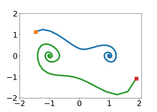
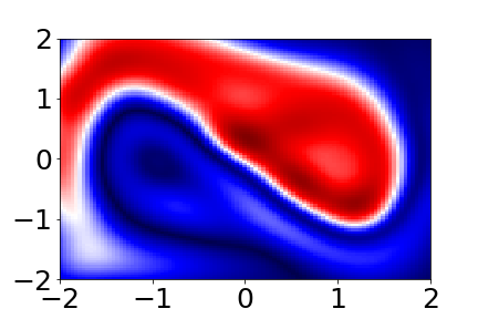
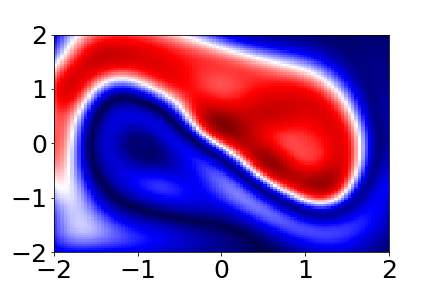
[]     [$\varepsilon=0$]     [$\varepsilon=2\eta^{3}$]     [$\varepsilon=1.5\eta^{2}$]

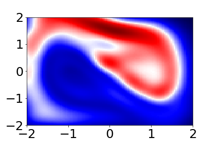
Figure 2: (a) Two trajectories of the Duffing oscillator that converge to two different equilibrium points. (b)-(d) Leading eigenfunction of ${\cal K}$ with eigenvalue $1$ at $t=3550$ under various compression budget with (b)$\varepsilon=0$,$|{\cal D}_{t}|=3550$, (c) $\varepsilon=2\eta^{3}$,$|{\cal D}_{t}|=300$, and (d) $\varepsilon=1.5\eta^{2}$,$|{\cal D}_{t}|=190$.

To approximate ${\cal K}$, the streaming data consists of samples from $355$ trajectories over region $[-2,2]\times[-2,2]$. We used a sampling interval of $0.25$s and did not require the sampled trajectories to be fully mixed. We utilized a Gaussian kernel $\kappa\left(x_{1},x_{2}\right)=\exp(-\|x_{1}-x_{2}\|^{2}_{2}/(2\times 0.3^{2}))$ and implemented Algorithm E with a constant step-size $\eta=0.2$ and processed $3550$ steaming sample pairs. Figure 2-2 portrays heat maps of the leading eigenfunctions of ${\cal K}$ after $3550$ iterations with various values of compression budget $\varepsilon$. Upon increasing $\varepsilon$, the dictionary becomes more compressed with fewer elements. As shown in Figure 2, the resulting eigenfunctions accurately reveal the distinct regions of attractions, even with merely $10\%$ of total data points. However, the characterization becomes less sound with higher $\varepsilon$ as the algorithm discards too many points.

6 Conclusions

In this paper, we have presented an algorithm that learns a compressed version of the CME incrementally. Then, we studied the convergence behavior of the last literate under Markovian sampling. We have applied this framework to analyzing unknown nonlinear dynamical systems. Numerical examples confirmed the effectiveness of the proposed mechanism.

From the standpoint of pure theoretical analysis, we want to extend our last iterate convergence in the mean square sense to almost sure guarantees and those with high probability, and investigate asymptotic behavior. We also want to study if the multiple variants of scalar-valued stochastic gradient descent can be extended to the operator setting. In addition, we will investigate extending a variety of compression schemes for function learning in RKHS to the operator setting, e.g., windowed retention of old points Kivinen et al. (2004), approximate linear dependence Engel et al. (2004), random Fourier features Rahimi and Recht (2007), Nyström method Rudi et al. (2015), and coherence-based sparsification Richard et al. (2008). In terms of conceptual directions for future work, perhaps our main interest lies in the generalization of the online compressed CME learning framework to the question of reinforcement learning through approaches mirroring those in Grunewalder et al. (2012). Another direction of interest is the online fusion of compressed CME estimates, where multiple agents maintain and communicate separate compressed estimates over a network.

Disclaimer: This paper was prepared for informational purposes in part by the Artificial Intelligence Research group of JPMorgan Chase $\&$ Co and its affiliates (“J.P. Morgan”) and is not a product of the Research Department of J.P. Morgan. J.P. Morgan makes no representation and warranty whatsoever and disclaims all liability, for the completeness, accuracy or reliability of the information contained herein. This document is not intended as investment research or investment advice, or a recommendation, offer or solicitation for the purchase or sale of any security, financial instrument, financial product or service, or to be used in any way for evaluating the merits of participating in any transaction, and shall not constitute a solicitation under any jurisdiction or to any person, if such solicitation under such jurisdiction or to such person would be unlawful.

Appendix A provides a brief introduction to the tensor product Hilbert spaces and Hilbert-Schmidt operators. Appendix B contains the supporting materials regarding operator-valued gradients introduced in Section 3. Appendix C includes results that will be useful in handling the hard learning scenario. Appendix G presents a pseudo-code of our main algorithm. This is then followed by Appendix F that provides detailed proof of theorems regarding the convergence results. In the rest of the appendix, we present a detailed description of implementing the algorithm.

Appendix A A Primer on Tensor Product Hilbert Space and Hilbert-Schmidt Operators

This appendix recalls some facts regarding tensor product Hilbert spaces and Hilbert-Schmidt operators. We refer the reader to (Aubin, 2011, Chapter 12) for details.

Consider two separable real-valued Hilbert spaces ${\cal H}_{1}$ and ${\cal H}_{2}$ defined on separable measurable spaces $\mathbb{X}$ and $\mathbb{Y}$, respectively. Let $\{e_{i}\}_{i\in\mathbb{N}}$ be an orthonormal basis (ONB) of ${\cal H}_{1}$. A bounded linear operator $A:{\cal H}_{1}\to{\cal H}_{2}$ is a Hilbert-Schmidt (HS) operator if $\sum_{i\in\mathbb{N}}\left\|Ae_{i}\right\|_{{\cal H}_{2}}^{2}<\infty$. The quantity $\left\|A\right\|_{{\textrm{HS}}}=\left(\sum_{i\in\mathbb{N}}\left\|Ae_{i}\right\|_{{\cal H}_{2}}^{2}\right)^{1/2}$ is the Hilbert-Schmidt norm of $A$ and is independent of the choice of the ONB. For two HS operators $A$ and $B$ from ${\cal H}_{1}$ to ${\cal H}_{2}$, their Hilbert–Schmidt inner product can be defined as

$$\left\langle A,B\right\rangle_{{\textrm{HS}}({\cal H}_{1},{\cal H}_{2})}={\textrm{Tr}}{(A^{*}B)}=\sum_{i\in\mathbb{N}}\left\langle Ae_{i},Be_{i}\right\rangle_{{\cal H}_{2}}.$$ (36)

In addition, for a Hilbert-Schmidt operator $A$ and a bounded linear operator $B$, we have

$$\left\|A\right\|_{\textrm{HS}}={\textrm{Tr}}{(A^{*}A)}^{1/2},$$ (37)

$$\left\|A\right\|_{\textrm{HS}}=\left\|A^{*}\right\|_{\textrm{HS}},$$ (38)

$$\left\|A\right\|_{\textrm{op}}\leq\left\|A\right\|_{\textrm{HS}},$$ (39)

$$\left\|BA\right\|_{\textrm{HS}}\leq\left\|B\right\|_{\textrm{op}}\left\|A\right\|_{\textrm{HS}},\quad\left\|AB\right\|_{\textrm{HS}}\leq\left\|A\right\|_{\textrm{HS}}\left\|B\right\|_{\textrm{op}},$$ (40)

where $A^{*}$ is the adjoint of $A$ and $\left\|A\right\|_{\textrm{op}}$ is the operator norm of $A$. Let $f\in{\cal H}_{1},g\in{\cal H}_{2}$, the tensor product $f\otimes g:{\cal H}_{2}\to{\cal H}_{1}$ can be viewed as the linear rank-one operator defined by $(f\otimes g)h=\left\langle h,g\right\rangle_{{\cal H}_{2}}f$ for all $h\in{\cal H}_{2}$. Thus, for any bounded linear operator $A$ from ${\cal H}_{1}$ to itself, we have

$$A\left(\left(f\otimes g\right)h\right)=A\left(\left\langle h,g\right\rangle_{{\cal H}_{2}}f\right)=\left\langle h,g\right\rangle_{{\cal H}_{2}}\left(Af\right)=\left(\left(Af\right)\otimes g\right)h,\quad f\in{\cal H}_{1},h\in{\cal H}_{2}.$$ (41)

That is,

$$A\left(f\otimes g\right)=\left(Af\right)\otimes g.$$ (42)

Furthermore, if $\{e_{i}\}_{i\in\mathbb{N}}$ is an orthonormal systems (ONS) of ${\cal H}_{1}$ and $\{e^{\prime}_{j}\}_{j\in\mathbb{N}}$ is an ONS of ${\cal H}_{2}$, then $\{e_{i}\otimes e^{\prime}_{j}\}_{i,j\in\mathbb{N}}$ is an ONS of ${\cal H}_{1}\otimes{\cal H}_{2}$.

Now consider $f\in{\cal H}_{1}$, $g\in{\cal H}_{2}$ and $A$ is an HS operator mapping from ${\cal H}_{2}$ to ${\cal H}_{1}$. Let $(e_{i})_{i\in\mathbb{N}}$ be an orthonormal basis of ${\cal H}_{2}$. Then we have the Fourier series expansion of $g\in{\cal H}_{2}$ as

$$g=\sum_{i\in\mathbb{N}}\left\langle g,e_{i}\right\rangle_{{\cal H}_{2}}e_{i}.$$ (43)

Therefore, using (36), we have

$$\begin{aligned} \left\langle f\otimes g,A\right\rangle_{{\textrm{HS}}}=&\sum_{i\in\mathbb{N}}\left\langle\left(f\otimes g\right)e_{i},Ae_{i}\right\rangle_{{\cal H}_{1}}\\ =&\sum_{i\in\mathbb{N}}\left\langle\left\langle g,e_{i}\right\rangle_{{\cal H}_{2}}f,Ae_{i}\right\rangle_{{\cal H}_{1}}\\ =&\sum_{i\in\mathbb{N}}\left\langle g,e_{i}\right\rangle_{{\cal H}_{2}}\left\langle f,Ae_{i}\right\rangle_{{\cal H}_{1}}\\ =&\sum_{i\in\mathbb{N}}\left\langle g,e_{i}\right\rangle_{{\cal H}_{2}}\left\langle A^{*}f,e_{i}\right\rangle_{{\cal H}_{2}}\\ =&\left\langle\left\{\left\langle g,e_{i}\right\rangle_{{\cal H}_{2}}\right\}_{i\in\mathbb{N}},\left\{\left\langle A^{*}f,e_{i}\right\rangle_{{\cal H}_{2}}\right\}_{i\in\mathbb{N}}\right\rangle_{l_{2}(\mathbb{N})}.\end{aligned}$$ (44)

Since a separable Hilbert space is isomorphic to $l_{2}(\mathbb{N})$ (Aubin, 2011, Theorem 1.7.2), let $T(g)=\left\{\left\langle g,e_{i}\right\rangle_{{\cal H}_{2}}\right\}_{i\in\mathbb{N}}$ denote such an isomorphism $T:{\cal H}_{2}\mapsto l_{2}(\mathbb{N})$ then we have

$$\begin{aligned} \left\langle f\otimes g,A\right\rangle_{{\textrm{HS}}}=\left\langle T(g),T(A^{*}f)\right\rangle_{l_{2}(\mathbb{N})}=\left\langle g,A^{*}f\right\rangle_{{\cal H}_{2}}=\left\langle f,Ag\right\rangle_{{\cal H}_{1}}.\end{aligned}$$ (45)

A.1 Proof of Lemma 2.1

For the first claim, (Ciliberto et al., 2016, Lemma 15) and (Li et al., 2022, Theorem 1) show that there exists an isometric isomorphism $\iota_{\kappa}:{\cal H}_{Y}\otimes{\cal H}_{X}\to{\cal H}_{V}$. Moreover, Li et al. (2022) further establishes that for each $v\in{\cal H}_{V}$, there exists a unique $V\in{\cal H}_{Y}\otimes{\cal H}_{X}$ given by $V=\iota_{\kappa}^{-1}(v)$ such that $\left\|v\right\|_{{\cal H}_{V}}=\left\|V\right\|_{\textrm{HS}}$ and the operator reproducing property holds, i.e.,

$$v(x)=V\phi_{X}(x)\in{\cal H}_{Y},\quad\forall x\in\mathbb{X}.$$ (46)

For the second claim, ${\cal H}_{Y}\otimes[{\cal H}_{X}]\subseteq{\cal H}_{Y}\otimes{L_{2}\left(\rho_{X}\right)}$. In addition, according to (Aubin, 2011, Theorem 12.6.1), there exists an isomorphism $\iota:L_{2}(\rho_{X},{\cal H}_{Y})\to{\cal H}_{Y}\otimes{L_{2}\left(\rho_{X}\right)}$ .

Appendix B Operator-valued Gradient and Its Properties

B.1 Proof of Lemma 3.1

Consider $R_{\lambda}:{\textrm{HS}}({\cal H}_{X},{\cal H}_{Y})\to\mathbb{R}$ in (7). For any $h\in\mathbb{R}$ and $U,U^{\prime}\in{\textrm{HS}}({\cal H}_{X},{\cal H}_{Y})$, we have

$$R_{\lambda}(U+hU^{\prime})=R_{\lambda}(U)+h\ \left\langle\nabla R_{\lambda}(U),U^{\prime}\right\rangle_{\textrm{HS}}+{\cal O}(h^{2}).$$ (47)

Hence,

$$\begin{aligned} \left\langle\nabla R_{\lambda}\left(U\right),U^{\prime}\right\rangle_{\textrm{HS}}&=\lim_{h\to 0}\frac{R_{\lambda}(U+hU^{\prime})-R_{\lambda}(U)}{h}\\ &=\underbrace{\lim_{h\to 0}\frac{1}{2h}\mathds{E}\left[\left\|\phi_{Y}(y)-U\phi_{X}(x)-hU^{\prime}\phi_{X}(x)\right\|_{{\cal H}_{Y}}^{2}-\left\|\phi_{Y}(y)-U\phi_{X}(x)\right\|_{{\cal H}_{Y}}^{2}\right]}_{T_{1}}\\ &+\underbrace{\lim_{h\to 0}\frac{\lambda\left\|U+hU^{\prime}\right\|^{2}_{{\textrm{HS}}}-\lambda\left\|U\right\|_{{\textrm{HS}}}^{2}}{2h}}_{T_{2}}.\end{aligned}$$ (48)

To compute $T_{1}$ , first notice that

$$\begin{aligned} &\frac{1}{2h}\mathds{E}\left[\left\|\phi_{Y}(y)-U\phi_{X}(x)-hU^{\prime}\phi_{X}(x)\right\|_{{\cal H}_{Y}}^{2}-\left\|\phi_{Y}(y)-U\phi_{X}(x)\right\|_{{\cal H}_{Y}}^{2}\right]\\ =&\mathds{E}\left[\frac{-2h\left\langle\phi_{Y}(y)-U\phi_{X}(x),U^{\prime}\phi_{X}(x)\right\rangle_{{\cal H}_{Y}}+\left\|hU^{\prime}\phi_{X}(x)\right\|_{{\cal H}_{Y}}^{2}}{2h}\right]\\ =&\mathds{E}\left[-\left\langle\phi_{Y}(y)-U\phi_{X}(x),U^{\prime}\phi_{X}(x)\right\rangle_{{\cal H}_{Y}}+\frac{h}{2}\left\|U^{\prime}\phi_{X}(x)\right\|_{{\cal H}_{Y}}^{2}\right].\end{aligned}$$ (49)

By Assumption 1, the kernel function is bounded. Since $U,U^{\prime}$ are Hilbert-Schmidt from ${\cal H}_{X}$ to ${\cal H}_{Y}$, we can apply the dominated convergence theorem to obtain

$$\begin{aligned} T_{1}=&\lim_{h\to 0}\mathds{E}\left[-\left\langle\phi_{Y}(y)-U\phi_{X}(x),U^{\prime}\phi_{X}(x)\right\rangle_{{\cal H}_{Y}}+\frac{h}{2}\left\|U^{\prime}\phi_{X}(x)\right\|_{{\cal H}_{Y}}^{2}\right]\\ =&\mathds{E}\left[-\left\langle\phi_{Y}(y)-U\phi_{X}(x),U^{\prime}\phi_{X}(x)\right\rangle_{{\cal H}_{Y}}\right].\end{aligned}$$ (50)

From (45), the last line above can be written as

$$\begin{aligned} T_{1}=&-\mathds{E}\left[\left\langle\left(\phi_{Y}(y)-U\phi_{X}(x)\right)\otimes\left(\phi_{X}(x)\right),U^{\prime}\right\rangle_{{\textrm{HS}}}\right]\\ =&-\left\langle\mathds{E}\left[\left(\phi_{Y}(y)-U\phi_{X}(x)\right)\otimes\left(\phi_{X}(x)\right)\right],U^{\prime}\right\rangle_{{\textrm{HS}}},\end{aligned}$$ (51)

Likewise for $T_{2}$, we have

$$\begin{aligned} T_{2}=\frac{\lambda}{2}\lim_{h\to 0}\frac{\left\|U+hU^{\prime}\right\|^{2}_{{\textrm{HS}}}-\left\|U\right\|_{{\textrm{HS}}}^{2}}{h}=\lambda\left\langle U,U^{\prime}\right\rangle_{\textrm{HS}}.\end{aligned}$$ (52)

Putting together, (48) becomes

$$\begin{aligned} \left\langle\nabla R_{\lambda}\left(U\right),U^{\prime}\right\rangle_{\textrm{HS}}=\left\langle-\mathds{E}\left[\left(\phi_{Y}(y)-U\phi_{X}(x)\right)\otimes\left(\phi_{X}(x)\right)\right]+\lambda U,U^{\prime}\right\rangle_{\textrm{HS}}.\end{aligned}$$ (53)

Hence, the operator gradient of $R_{\lambda}(U)$ is given by

$$\begin{aligned} \nabla R_{\lambda}(U)=&-\mathds{E}\left[\left(\phi_{Y}(y)-U\phi_{X}(x)\right)\otimes\left(\phi_{X}(x)\right)\right]+\lambda U\\ =&UC_{XX}-C_{YX}+\lambda U.\end{aligned}$$ (54)

In addition, since $C_{XX}$,$C_{YX}$ is Hilbert Schmidt when the kernel function is uniformly bounded Fukumizu et al. (2004), we get that $\nabla R_{\lambda}(U)\in{\textrm{HS}}({\cal H}_{X},{\cal H}_{Y})$, which completes the proof.

B.2 Properties of Operator-valued Gradients

Consider $(x,y)\in\mathbb{X}\times\mathbb{Y}$ and define

$$\widetilde{C}_{XX}(x) =\phi_{X}\left(x\right)\otimes\phi_{X}\left(x\right),$$

$$\widetilde{C}_{YX}(y,x) =\phi_{Y}\left(y\right)\otimes\phi_{X}\left(x\right)$$

Under Assumption 1(i), we have

$$\begin{aligned} \left\|\widetilde{C}_{XX}(x)\right\|^{2}_{\textrm{HS}}&=\left\langle\phi_{X}\left(x\right)\otimes\phi_{X}\left(x\right),\phi_{X}\left(x\right)\otimes\phi_{X}\left(x\right)\right\rangle_{\textrm{HS}}=\kappa_{X}(x,x)\kappa_{X}(x,x)\leq K^{2}\\ \left\|\widetilde{C}_{YX}(y,x)\right\|^{2}_{\textrm{HS}}&=\left\langle\phi_{Y}\left(y\right)\otimes\phi_{X}\left(x\right),\phi_{Y}\left(y\right)\otimes\phi_{X}\left(x\right)\right\rangle_{\textrm{HS}}=\kappa_{X}(x,x)\kappa_{Y}(y,y)\leq K^{2}.\end{aligned}$$ (55)

Let $B_{\kappa}=K+\lambda$. Then,

$$\begin{aligned} &\max_{x\in\mathbb{X}}\left\|\widetilde{C}_{XX}(x)+\lambda{\textrm{Id}}\right\|_{\textrm{op}}\leq\max_{x\in\mathbb{X}}\left(\left\|\widetilde{C}_{XX}(x)\right\|_{\textrm{op}}+\lambda\left\|{\textrm{Id}}\right\|_{\textrm{op}}\right)\leq\max_{x\in\mathbb{X}}\left(\left\|\widetilde{C}_{XX}(x)\right\|_{\textrm{HS}}\right)+\lambda\leq B_{\kappa}\\ &\max_{x\in\mathbb{X},y\in\mathbb{Y}}\left\|\widetilde{C}_{YX}(y,x)\right\|_{\textrm{HS}}\leq K\leq B_{\kappa}.\end{aligned}$$ (56)

We have the following properties regarding $\nabla R_{\lambda}(U)$,$\widetilde{\nabla}R_{\lambda}(x,y,U)$ which are needed for the convergence analysis.

Lemma B.1.

(Properties of gradients) Under Assumptions 1 and 2, $\nabla R_{\lambda}(U)$ and its stochastic approximation $\widetilde{\nabla}R_{\lambda}(x,y,U)$ satisfy the following.

1. (Strong convexity) For $U\in{\textrm{HS}}\left({\cal H}_{X},{\cal H}_{Y}\right)$,

   $$\left\langle-\nabla R_{\lambda}(U),U-U_{\lambda}\right\rangle_{\textrm{HS}}\leq-\lambda\left\|U-U_{\lambda}\right\|_{\textrm{HS}}^{2},$$

   where $U_{\lambda}:=\mathop{\rm argmin}_{U\in{\textrm{HS}}({\cal H}_{X},{\cal H}_{Y})}R_{\lambda}(U)$.

2. (Lipschitz gradient) $\nabla R_{\lambda}(U)$ and $\widetilde{\nabla}R_{\lambda}(x,y,U)$ are Lipschitz continuous with respect to $U$ for all $x\in\mathbb{X},y\in\mathbb{Y}$, i.e.,

   $$\left\|\nabla R_{\lambda}(U_{1})-\nabla R_{\lambda}(U_{2})\right\|_{\textrm{HS}} \leq B_{\kappa}\left\|U_{1}-U_{2}\right\|_{\textrm{HS}}$$

   $$\left\|\widetilde{\nabla}R_{\lambda}(x,y,U_{1})-\widetilde{\nabla}R_{\lambda}(x,y,U_{2})\right\|_{\textrm{HS}} \leq B_{\kappa}\left\|U_{1}-U_{2}\right\|_{\textrm{HS}}$$

   for all $U_{1},U_{2}\in{\textrm{HS}}\left({\cal H}_{X},{\cal H}_{Y}\right)$ and $x\in\mathbb{X},y\in\mathbb{Y}$.

3. (Affine scaling) For $U\in{\textrm{HS}}\left({\cal H}_{X},{\cal H}_{Y}\right)$,

   $$\left\|\nabla R_{\lambda}\left(U\right)\right\|_{\textrm{HS}} \leq B_{\kappa}\left(\left\|U\right\|_{\textrm{HS}}+1\right)$$

   $$\left\|\widetilde{\nabla}R_{\lambda}\left(x,y,U\right)\right\|_{\textrm{HS}} \leq B_{\kappa}\left(\left\|U\right\|_{\textrm{HS}}+1\right)$$

   for all $x\in\mathbb{X},y\in\mathbb{Y}$. As a result, $\nabla R_{\lambda}\left(U\right)$ and $\widetilde{\nabla}R_{\lambda}\left(x,y,U\right)$ are Bochner-integrable.

Proof B.2.

Denote $g(U):=R_{\lambda}(U)-\frac{\lambda}{2}\left\|U\right\|_{{\textrm{HS}}}^{2}$. Then for $U_{1},U_{2}\in{\textrm{HS}}({\cal H}_{X},{\cal H}_{Y})$ and $\alpha\in(0,1]$,

$$\begin{aligned} g\left(\alpha U_{1}+\left(1-\alpha\right)U_{2}\right)=&\frac{1}{2}\mathds{E}\left[\left\|\phi_{Y}(y)-\left(\alpha U_{1}+\left(1-\alpha\right)U_{2}\right)\phi_{X}(x)\right\|_{{\cal H}_{Y}}^{2}\right]\\ =&\frac{1}{2}\mathds{E}\left[\left\|\left(\alpha+\left(1-\alpha\right)\right)\phi_{Y}(y)-\left(\alpha U_{1}+\left(1-\alpha\right)U_{2}\right)\phi_{X}(x)\right\|_{{\cal H}_{Y}}^{2}\right]\\ =&\frac{1}{2}\mathds{E}\left[\left\|\alpha\left(\phi_{Y}(y)-U_{1}\phi_{X}(x)\right)+\left(1-\alpha\right)\left(\phi_{Y}(y)-U_{2}\phi_{X}(x)\right)\right\|_{{\cal H}_{Y}}^{2}\right].\end{aligned}$$ (57)

Let $T_{1}:=\phi_{Y}(y)-U_{1}\phi_{X}(x)$ and $T_{2}:=\phi_{Y}(y)-U_{2}\phi_{X}(x)$. Then, we have

$$\begin{aligned} g\left(\alpha U_{1}+\left(1-\alpha\right)U_{2}\right)&=\frac{1}{2}\mathds{E}\left\|\alpha T_{1}+\left(1-\alpha\right)T_{2}\right\|_{{\cal H}_{Y}}^{2}\\ &=\frac{1}{2}\mathds{E}\left[\alpha^{2}\left\|T_{1}\right\|_{{\cal H}_{Y}}^{2}+\left(1-\alpha\right)^{2}\left\|T_{2}\right\|_{{\cal H}_{Y}}^{2}+2\alpha\left(1-\alpha\right)\left\langle T_{1},T_{2}\right\rangle_{{\cal H}_{Y}}\right].\end{aligned}$$ (58)

Hence, for $\alpha\in(0,1]$, we have

$$\begin{aligned} &\alpha g\left(U_{1}\right)+\left(1-\alpha\right)g\left(U_{2}\right)-g\left(\alpha U_{1}+\left(1-\alpha\right)U_{2}\right)\\ =&\frac{\alpha}{2}\mathds{E}\left\|T_{1}\right\|_{{\cal H}_{Y}}^{2}+\frac{1-\alpha}{2}\mathds{E}\left\|T_{2}\right\|_{{\cal H}_{Y}}^{2}-\frac{1}{2}\mathds{E}\left\|\alpha T_{1}+\left(1-\alpha\right)T_{2}\right\|_{{\cal H}_{Y}}^{2}\\ =&\frac{1}{2}\mathds{E}\left[\alpha\left(1-\alpha\right)\left\|T_{1}\right\|_{{\cal H}_{Y}}^{2}+\alpha\left(1-\alpha\right)\left\|T_{2}\right\|_{{\cal H}_{Y}}^{2}-2\alpha\left(1-\alpha\right)\left\langle T_{1},T_{2}\right\rangle_{{\cal H}_{Y}}\right]\\ =&\frac{\alpha\left(1-\alpha\right)}{2}\mathds{E}\left[\left\|T_{1}\right\|_{{\cal H}_{Y}}^{2}+\left\|T_{2}\right\|_{{\cal H}_{Y}}^{2}-2\left\langle T_{1},T_{2}\right\rangle_{{\cal H}_{Y}}\right]\\ =&\frac{\alpha\left(1-\alpha\right)}{2}\mathds{E}\left[\left\|T_{1}-T_{2}\right\|_{{\cal H}_{Y}}^{2}\right]\\ \geq&0.\end{aligned}$$ (59)

That is, $g:{\textrm{HS}}({\cal H}_{X},{\cal H}_{Y})\to\mathbb{R}$ satisfies

$$g\left(\alpha U_{1}+\left(1-\alpha\right)U_{2}\right)\leq\alpha g\left(U_{1}\right)+\left(1-\alpha\right)g\left(U_{2}\right),$$ (60)

and thus is a convex functional in the sense of (Luenberger, 1997, p. 190). Rearranging terms in the above equation, we have

$$\begin{aligned} g\left(U_{1}\right)-g\left(U_{2}\right)\geq\frac{g\left(U_{2}+\alpha\left(U_{1}-U_{2}\right)\right)-g\left(U_{2}\right)}{\alpha},\quad\alpha\in(0,1].\end{aligned}$$ (61)

Taking $\alpha\to 0$, we have

$$\begin{aligned} g\left(U_{1}\right)-g\left(U_{2}\right)\geq&\lim_{\alpha\to 0}\frac{g\left(U_{2}+\alpha\left(U_{1}-U_{2}\right)\right)-g\left(U_{2}\right)}{\alpha}\\ =&\left\langle\nabla g\left(U_{2}\right),U_{1}-U_{2}\right\rangle_{\textrm{HS}},\end{aligned}$$ (62)

where the last line holds due to $\eqref{eq.OSDG-exp}$ by replacing $R_{\lambda}(\cdot)$ with $g(\cdot)$. Now, substituting $g(\cdot)$ with $R_{\lambda}(\cdot)-\frac{\lambda}{2}\left\|\cdot\right\|_{{\textrm{HS}}}^{2}$, we have for $U_{1},U_{2}\in{\textrm{HS}}({\cal H}_{X},{\cal H}_{Y})$,

$$\begin{aligned} \left[R_{\lambda}\left(U_{1}\right)-\frac{\lambda}{2}\left\|U_{1}\right\|_{\textrm{HS}}^{2}\right]-\left[R_{\lambda}\left(U_{2}\right)-\frac{\lambda}{2}\left\|U_{2}\right\|_{\textrm{HS}}^{2}\right]\geq&\left\langle\nabla R_{\lambda}\left(U_{2}\right)-\lambda U_{2},U_{1}-U_{2}\right\rangle_{\textrm{HS}}.\end{aligned}$$ (63)

Rearranging terms gives

$$\begin{aligned} R_{\lambda}\left(U_{1}\right)-R_{\lambda}\left(U_{2}\right)\geq&\left\langle\nabla R_{\lambda}\left(U_{2}\right),U_{1}-U_{2}\right\rangle_{\textrm{HS}}-\lambda\left\langle U_{2},U_{1}-U_{2}\right\rangle_{\textrm{HS}}+\frac{\lambda}{2}\left\|U_{1}\right\|_{\textrm{HS}}^{2}-\frac{\lambda}{2}\left\|U_{2}\right\|_{\textrm{HS}}^{2}\\ =&\left\langle\nabla R_{\lambda}\left(U_{2}\right),U_{1}-U_{2}\right\rangle_{\textrm{HS}}-\lambda\left\langle U_{2},U_{1}\right\rangle_{\textrm{HS}}+\frac{\lambda}{2}\left\|U_{1}\right\|_{\textrm{HS}}^{2}+\frac{\lambda}{2}\left\|U_{2}\right\|_{\textrm{HS}}^{2}\\ =&\left\langle\nabla R_{\lambda}\left(U_{2}\right),U_{1}-U_{2}\right\rangle_{\textrm{HS}}+\frac{\lambda}{2}\left\|U_{1}-U_{2}\right\|_{\textrm{HS}}^{2}.\end{aligned}$$ (64)

In other words, $R_{\lambda}$ is $\lambda$-strongly convex. From (64), we have for $U_{1},U_{2}\in{\textrm{HS}}({\cal H}_{X},{\cal H}_{Y})$,

$$\begin{aligned} R_{\lambda}\left(U_{1}\right)-R_{\lambda}\left(U_{2}\right)\geq&\left\langle\nabla R_{\lambda}\left(U_{2}\right),U_{1}-U_{2}\right\rangle_{\textrm{HS}}+\frac{\lambda}{2}\left\|U_{1}-U_{2}\right\|^{2}_{\textrm{HS}},\\ R_{\lambda}\left(U_{2}\right)-R_{\lambda}\left(U_{1}\right)\geq&\left\langle\nabla R_{\lambda}\left(U_{1}\right),U_{2}-U_{1}\right\rangle_{\textrm{HS}}+\frac{\lambda}{2}\left\|U_{1}-U_{2}\right\|^{2}_{\textrm{HS}}.\end{aligned}$$ (65)

Adding these two we have

$$\begin{aligned} 0\geq&\left\langle\nabla R_{\lambda}\left(U_{2}\right)-\nabla R_{\lambda}\left(U_{1}\right),U_{1}-U_{2}\right\rangle_{\textrm{HS}}+\lambda\left\|U_{1}-U_{2}\right\|_{\textrm{HS}}^{2}.\end{aligned}$$ (66)

Let $U_{1}=U$, $U_{2}=U_{\lambda}$. Since $\nabla R_{\lambda}\left(U_{\lambda}\right)=0$, we have

$$\begin{aligned} 0\geq&\left\langle-\nabla R_{\lambda}\left(U_{1}\right),U_{1}-U_{\lambda}\right\rangle_{\textrm{HS}}+\lambda\left\|U_{1}-U_{2}\right\|_{\textrm{HS}}^{2}.\end{aligned}$$ (67)

Rearranging terms concludes the proof of claim (a).

To prove the second and third claims, we have

$$\begin{aligned} &\left\|\widetilde{\nabla}R_{\lambda}(x,y,U_{1})-\widetilde{\nabla}R_{\lambda}(x,y,U_{2})\right\|_{\textrm{HS}}\\ =&\left\|\left[U_{1}\widetilde{C}_{XX}(x)-\widetilde{C}_{YX}(y,x)+\lambda U_{1}\right]-\left[U_{2}\widetilde{C}_{XX}(x)-\widetilde{C}_{YX}(y,x)+\lambda U_{2}\right]\right\|_{\textrm{HS}}\\ =&\left\|\left(U_{1}-U_{2}\right)\left(\widetilde{C}_{XX}(x)+\lambda{\textrm{Id}}\right)\right\|_{\textrm{HS}}.\end{aligned}$$ (68)

Using the fact that $\left\|AB\right\|_{\textrm{HS}}\leq\left\|A\right\|_{\textrm{HS}}\left\|B\right\|_{\textrm{op}}$ for Hilbert-Schmidt operator $A$ and bounded linear operator $B$, we further have

$$\begin{aligned} \left\|\widetilde{\nabla}R_{\lambda}(x,y,U_{1})-\widetilde{\nabla}R_{\lambda}(x,y,U_{2})\right\|_{\textrm{HS}}\leq&\left\|U_{1}-U_{2}\right\|_{\textrm{HS}}\left\|\widetilde{C}_{XX}(x)+\lambda{\textrm{Id}}\right\|_{\textrm{op}}\\ \leq&B_{\kappa}\left\|U_{1}-U_{2}\right\|_{\textrm{HS}}.\end{aligned}$$ (69)

Together with triangle inequality w.r.t HS-norm, we then have

$$\begin{aligned} \left\|\widetilde{\nabla}R_{\lambda}\left(x,y,U\right)\right\|_{\textrm{HS}}\leq&\left\|\widetilde{\nabla}R_{\lambda}\left(x,y,U\right)-\widetilde{\nabla}R_{\lambda}\left(x,y,0\right)\right\|_{\textrm{HS}}+\left\|\widetilde{\nabla}R_{\lambda}\left(x,y,0\right)\right\|_{\textrm{HS}}\\ \leq&B_{\kappa}\left\|U\right\|_{\textrm{HS}}+\left\|\widetilde{C}_{YX}(y,x)\right\|_{\textrm{HS}}\\ \leq&B_{\kappa}\left(\left\|U\right\|_{\textrm{HS}}+1\right).\end{aligned}$$ (70)

Since $U$ is Hilbert-Schmdit, the above inequality also implies that $\int_{\mathbb{X}\times\mathbb{Y}}\left\|\widetilde{\nabla}R_{\lambda}\left(x,y,U\right)\right\|_{\textrm{HS}}\mathrm{d}\rho\left(x,y\right)\leq B_{\kappa}\left(\left\|U\right\|_{\textrm{HS}}+1\right)<\infty$, i.e., $\widetilde{\nabla}R_{\lambda}\left(x,y,U\right)$ is Bochner-integrable. Using Jensen’s inequality, we have

$$\begin{aligned} \left\|\nabla R_{\lambda}\left(U\right)\right\|_{\textrm{HS}}&=\left\|\mathds{E}\left[\widetilde{\nabla}R_{\lambda}\left(x,y,U\right)\right]\right\|_{\textrm{HS}}\\ &\leq\mathds{E}\left[\left\|\widetilde{\nabla}R_{\lambda}\left(x,y,U\right)\right\|_{\textrm{HS}}\right]\\ &\leq B_{\kappa}\left(\left\|U\right\|_{\textrm{HS}}+1\right).\end{aligned}$$ (71)

Similarly, using (69), we get

$$\begin{aligned} \left\|\nabla R_{\lambda}(U_{1})-\nabla R_{\lambda}(U_{2})\right\|_{\textrm{HS}}=&\left\|\mathds{E}\left[\widetilde{\nabla}R_{\lambda}(x,y,U_{1})-\widetilde{\nabla}R_{\lambda}(x,y,U_{2})\right]\right\|_{\textrm{HS}}\\ \leq&\mathds{E}\left[\left\|\widetilde{\nabla}R_{\lambda}(x,y,U_{1})-\widetilde{\nabla}R_{\lambda}(x,y,U_{2})\right\|_{\textrm{HS}}\right]\\ \leq&B_{\kappa}\left\|U_{1}-U_{2}\right\|_{\textrm{HS}}.\end{aligned}$$ (72)

Appendix C Technical Lemmas Related to Learning in the Power Spaces

By spectral theorem, the integral operator $L_{\kappa}$ defined in (20) enjoys the spectral representation (21) which is convergent in ${L_{2}\left(\rho_{X}\right)}$. Since $L_{\kappa}$ is a strictly positive operator, then for any $r\in[0,\infty)$, the fractional power $L_{\kappa}^{r}:{L_{2}\left(\rho_{X}\right)}\to{L_{2}\left(\rho_{X}\right)}$ is defined by

$$L_{\kappa}^{r}[f]:=\sum_{i\in\mathbb{I}}\sigma_{i}^{r}\left\langle[f],[e_{i}]\right\rangle_{\rho}[e_{i}],\quad[f]\in{L_{2}\left(\rho_{X}\right)}.$$ (73)

Moreover, define the adjoint of ${I_{\kappa}}$ by ${I_{\kappa}}^{*}:{L_{2}\left(\rho_{X}\right)}\to{\cal H}$. From the adjoint relation, we have for any $f\in{L_{2}\left(\rho_{X}\right)}$ and $h\in{\cal H}$

$$\left\langle{I_{\kappa}}^{*}[f],h\right\rangle_{\cal H}=\left\langle[f],{I_{\kappa}}h\right\rangle_{\rho}=\int_{\mathbb{X}}g(x)\ h(x)\mathrm{d}\rho_{X}(x)\quad\forall g\in[f].$$ (74)

Taking $h=\kappa(\cdot,x)=:\kappa_{x}$ for $x\in X$ yields that

$${I_{\kappa}}^{*}[f]=\int_{\mathbb{X}}\kappa(\cdot,x)g(x)\mathrm{d}\rho_{X}\quad\forall g\in[f].$$ (75)

In addition, since $\left(\kappa_{x}\otimes\kappa_{x}\right)h=\left\langle h,\kappa_{x}\right\rangle_{\cal H}\kappa_{x}$, for all $h\in{\cal H}$, we have

$${\small\begin{aligned} {C_{\kappa}}h=({I_{\kappa}}^{*}{I_{\kappa}})h={I_{\kappa}}^{*}({I_{\kappa}}h)=\int_{\mathbb{X}}\kappa_{x}h(x)\mathrm{d}\rho_{X}(x)=\int_{\mathbb{X}}\kappa_{x}\left\langle h,\kappa_{x}\right\rangle_{\cal H}\mathrm{d}\rho_{X}(x)=\int_{\mathbb{X}}\left(\kappa_{x}\otimes\kappa_{x}\right)h\mathrm{d}\rho_{X}(x).\end{aligned}}$$ (76)

That is, the self-adjoint integral operator ${C_{\kappa}}:={I_{\kappa}}^{*}{I_{\kappa}}$ is the covariance operator $C_{XX}$ defined in Section 2.3 with respect to the probability measure $\rho_{X}$.

Recall that $\left(\sigma_{i}^{1/2}e_{i}\right)_{i\in\mathbb{I}}$ is an ONB of $\left(\ker{I_{\kappa}}\right)^{\perp}$, $\left([{e}_{i}]\right)_{i\in\mathbb{I}}$ an ONB of $\overline{\text{range}{I_{\kappa}}}$, and we have the spectral representation of ${C_{\kappa}}$ with respect to the ONS $\left(\sqrt{\sigma_{i}}e_{i}\right)_{i\in\mathbb{I}}$ in ${\cal H}$.

$${C_{\kappa}}=\sum_{i\in\mathbb{I}}\sigma_{i}\left\langle\cdot,\sqrt{\sigma_{i}}e_{i}\right\rangle_{\cal H}\sqrt{\sigma_{i}}e_{i},\quad{\cal H}=\ker{C_{\kappa}}\oplus\overline{\text{span}\left(e_{i},i\in\mathbb{I}\right)}.$$ (77)

In addition, ${I_{\kappa}}^{*}$ also admits the spectral decomposition

$${I_{\kappa}}^{*}=\sum_{i\in\mathbb{I}}\sigma_{i}\left\langle\cdot,[e_{i}]\right\rangle_{\rho}e_{i},$$ (78)

per (Steinwart and Scovel, 2012, Theorem 2.11).

Recall that $\left(\sigma_{i}^{1/2}e_{i}\right)_{i\in\mathbb{I}}$ is an ONB of $\left(\ker{I_{\kappa}}\right)^{\perp}$, $\left([{e}_{i}]\right)_{i\in\mathbb{I}}$ an ONB of $\overline{\text{range}{I_{\kappa}}}$. Since every ONS can be extended to an ONB, let $\left(\widetilde{e}_{i}\right)_{i\in\mathbb{J}}$ be an ONB of $\ker{I_{\kappa}}$ with $\mathbb{J}\cap\mathbb{N}=\varnothing$ such that $\left(\sigma_{i}^{1/2}e_{i}\right)_{i\in\mathbb{I}}\cup\left(\widetilde{e}_{i}\right)_{i\in\mathbb{J}}$ is an ONB of ${\cal H}_{X}$. We then have the spectral representation for $0\leq\gamma\leq 1$ and $a>0$,

$${C_{\kappa}}^{\frac{1-\gamma}{2}}= \sum_{i\in\mathbb{I}}\sigma_{i}^{\frac{1-\gamma}{2}}\left\langle\cdot,\sigma_{i}^{1/2}e_{i}\right\rangle_{\cal H}\sigma_{i}^{1/2}e_{i},$$ (79)

$$\left({C_{\kappa}}+\lambda{\textrm{Id}}\right)^{-a}= \sum_{i\in\mathbb{I}}\left(\sigma_{i}+\lambda\right)^{-a}\left\langle\sigma_{i}^{1/2}e_{i},\cdot\right\rangle_{\cal H}\sigma_{i}^{1/2}e_{i}+\lambda^{-a}\sum_{j\in\mathbb{J}}\left\langle\widetilde{e}_{j},\cdot\right\rangle_{\cal H}\widetilde{e}_{j},$$ (80)

per Fischer and Steinwart (2020). Based on the above spectral representations, we derive the bound bound below which will be useful later. By the definition of operator norm, we have

$$\begin{aligned} \left\|{C_{\kappa}}^{\frac{1-\gamma}{2}}\left({C_{\kappa}}+\lambda{\textrm{Id}}\right)^{-1/2}\right\|_{\textrm{op}}^{2}=&\sup_{\left\|f\right\|_{\cal H}=1}\left\|{C_{\kappa}}^{\frac{1-\gamma}{2}}\left({C_{\kappa}}+\lambda{\textrm{Id}}\right)^{-1/2}f\right\|_{\cal H}^{2},\end{aligned}$$ (81)

We next expand ${C_{\kappa}}^{\frac{1-\gamma}{2}}\left({C_{\kappa}}+\lambda{\textrm{Id}}\right)^{-1/2}$ based on (79), (80), and we have

$$\begin{aligned} &\left\|{C_{\kappa}}^{\frac{1-\gamma}{2}}\left({C_{\kappa}}+\lambda{\textrm{Id}}\right)^{-1/2}f\right\|_{\cal H}^{2}\\ =&\left\|\sum_{i\in\mathbb{I}}\sigma_{i}^{\frac{1-\gamma}{2}}\left\langle\sum_{i^{\prime}\in\mathbb{I}}\left(\sigma_{i^{\prime}}+\lambda\right)^{-1/2}\left\langle\sigma_{i^{\prime}}^{1/2}e_{i^{\prime}},f\right\rangle\sigma_{i^{\prime}}^{1/2}e_{i^{\prime}}+\lambda^{-1/2}\sum_{j\in\mathbb{J}}\left\langle\widetilde{e}_{j},f\right\rangle_{\cal H}\widetilde{e}_{j}\ ,\ \sigma_{i}^{1/2}e_{i}\right\rangle_{\cal H}\sigma_{i}^{1/2}e_{i}\right\|_{\cal H}^{2}\\ \stackrel{{\scriptstyle(a)}}{{=}}&\left\|\sum_{i\in\mathbb{I}}\sigma_{i}^{\frac{1-\gamma}{2}}\left(\sigma_{i}+\lambda\right)^{-1/2}\left\langle\sigma_{i}^{1/2}e_{i},f\right\rangle_{\cal H}\sigma_{i}^{1/2}e_{i}\right\|_{\cal H}^{2}\\ =&\sum_{i\in\mathbb{I}}\sum_{i^{\prime}\in\mathbb{I}}\left\langle\sigma_{i}^{\frac{1-\gamma}{2}}\left(\sigma_{i}+\lambda\right)^{-1/2}\left\langle\sigma_{i}^{1/2}e_{i},f\right\rangle_{\cal H}\sigma_{i}^{1/2}e_{i}\ ,\ \sigma_{i^{\prime}}^{\frac{1-\gamma}{2}}\left(\sigma_{i^{\prime}}+\lambda\right)^{-1/2}\left\langle\sigma_{i^{\prime}}^{1/2}e_{i^{\prime}},f\right\rangle_{\cal H}\sigma_{i^{\prime}}^{1/2}e_{i^{\prime}}\right\rangle_{\cal H}\\ =&\sum_{i\in\mathbb{I}}\sum_{i^{\prime}\in\mathbb{I}}\sigma_{i}^{\frac{1-\gamma}{2}}\left(\sigma_{i}+\lambda\right)^{-1/2}\sigma_{i^{\prime}}^{\frac{1-\gamma}{2}}\left(\sigma_{i^{\prime}}+\lambda\right)^{-1/2}\left\langle\sigma_{i}^{1/2}e_{i},f\right\rangle_{\cal H}\left\langle\sigma_{i^{\prime}}^{1/2}e_{i^{\prime}},f\right\rangle_{\cal H}\left\langle\sigma_{i}^{1/2}e_{i},\sigma_{i^{\prime}}^{1/2}e_{i^{\prime}}\right\rangle_{\cal H}\\ =&\sum_{i\in\mathbb{I}}\frac{\sigma_{i}^{1-\gamma}}{\sigma_{i}+\lambda}\left|\left\langle\sigma_{i}^{1/2}e_{i},f\right\rangle_{\cal H}\right|^{2}.\end{aligned}$$ (82)

In deriving the above expression, (a) holds since $\left(\sigma_{i}^{1/2}e_{i}\right)_{i\in\mathbb{I}}$ is an ONB of $\left(\ker{I_{\kappa}}\right)^{\perp}$ and $\left(\widetilde{e}_{i}\right)_{i\in\mathbb{J}}$ is an ONB of $\ker{I_{\kappa}}$. Therefore, we have

$$\begin{aligned} \left\|{C_{\kappa}}^{\frac{1-\gamma}{2}}\left({C_{\kappa}}+\lambda{\textrm{Id}}\right)^{-1/2}f\right\|_{\cal H}^{2}=&\sup_{\left\|f\right\|_{\cal H}=1}\sum_{i\in\mathbb{I}}\frac{\sigma_{i}^{1-\gamma}}{\sigma_{i}+\lambda}\left|\left\langle\sigma_{i}^{1/2}e_{i},f\right\rangle_{\cal H}\right|^{2}\\ \leq&\sup_{\left\|f\right\|_{\cal H}=1}\left(\sup_{i\in\mathbb{I}}\frac{\sigma_{i}^{1-\gamma}}{\sigma_{i}+\lambda}\right)\sum_{i\in\mathbb{I}}\left|\left\langle\sigma_{i}^{1/2}e_{i},f\right\rangle_{\cal H}\right|^{2}\\ \stackrel{{\scriptstyle(a)}}{{=}}&\sup_{\left\|f\right\|_{\cal H}=1}\left(\sup_{i\in\mathbb{I}}\frac{\sigma_{i}^{1-\gamma}}{\sigma_{i}+\lambda}\right)\left\|f\right\|_{\cal H}^{2}\\ =&\sup_{i\in\mathbb{I}}\frac{\sigma_{i}^{1-\gamma}}{\sigma_{i}+\lambda}\\ \leq&\lambda^{-\gamma},\end{aligned}$$ (83)

where (a) follows from the Parseval’s identity.

C.1 Bounding the $\gamma$-norm

We next introduce the following lemma that upper bound the $\gamma$-norm using the HS-norm.

Lemma C.1.

For $u\in{\cal H}_{V}$, let $U=\iota_{\kappa}^{-1}(u)\in{\textrm{HS}}({\cal H}_{X},{\cal H}_{Y})$, where $\iota_{\kappa}$ is the linear isomorphism in Lemma 2.1. For any $\gamma\in[0,1]$ and $U\in{\textrm{HS}}({\cal H}_{X},{\cal H}_{Y})$, we have

$$\begin{aligned} \left\|\left[u\right]\right\|_{\gamma}^{2}\leq\lambda^{-\left(\gamma+1\right)}\left(K+\lambda\right)^{2}\left\|U\right\|_{\textrm{HS}}^{2}.\end{aligned}$$ (84)

Proof C.2.

By (Li et al., 2022, Lemma 2), we have

$$\left\|\left[u\right]\right\|_{\gamma}\leq\left\|UC_{XX}^{\frac{1-\gamma}{2}}\right\|_{\textrm{HS}}.$$ (85)

First, notice that for a self-adjoint invertible operator $A$, $A^{-1/2}\times A\times A^{-1/2}={\textrm{Id}}$. Thus we have

$$\begin{aligned} UC_{XX}^{\frac{1-\gamma}{2}}=U\left(C_{XX}+\lambda{\textrm{Id}}\right)^{-1/2}\left(C_{XX}+\lambda{\textrm{Id}}\right)^{1/2}\left(C_{XX}+\lambda{\textrm{Id}}\right)^{1/2}\left(C_{XX}+\lambda{\textrm{Id}}\right)^{-1/2}C_{XX}^{\frac{1-\gamma}{2}}.\end{aligned}$$ (86)

Repeatedly applying (40) twice, we get

$$\begin{aligned} \left\|UC_{XX}^{\frac{1-\gamma}{2}}\right\|_{\textrm{HS}}^{2}=&\left\|U\left(C_{XX}+\lambda{\textrm{Id}}\right)^{-1/2}\left(C_{XX}+\lambda{\textrm{Id}}\right)\left(C_{XX}+\lambda{\textrm{Id}}\right)^{-1/2}C_{XX}^{\frac{1-\gamma}{2}}\right\|_{\textrm{HS}}^{2}\\ \leq&\left\|U\left(C_{XX}+\lambda{\textrm{Id}}\right)^{-1/2}\left(C_{XX}+\lambda{\textrm{Id}}\right)\right\|_{\textrm{HS}}^{2}\left\|\left(C_{XX}+\lambda{\textrm{Id}}\right)^{-1/2}C_{XX}^{\frac{1-\gamma}{2}}\right\|_{\textrm{op}}^{2}\\ \leq&\left\|U\left(C_{XX}+\lambda{\textrm{Id}}\right)^{-1/2}\right\|_{\textrm{HS}}^{2}\times\left\|C_{XX}+\lambda{\textrm{Id}}\right\|_{\textrm{op}}^{2}\times\left\|\left(C_{XX}+\lambda{\textrm{Id}}\right)^{-1/2}C_{XX}^{\frac{1-\gamma}{2}}\right\|_{\textrm{op}}^{2}.\end{aligned}$$ (87)

We can upper bound the second term in in (87) as follows:

$$\left\|C_{XX}+\lambda{\textrm{Id}}\right\|_{\textrm{op}}^{2}\leq\left(\left\|C_{XX}\right\|_{\textrm{op}}+\lambda\right)^{2}\leq\left(\left\|C_{XX}\right\|_{\textrm{HS}}+\lambda\right)^{2}\leq\left(K+\lambda\right)^{2}.$$ (88)

For the last term, by the self-adjointness of $C_{XX}$, we have

$$\left\|\left(C_{XX}+\lambda{\textrm{Id}}\right)^{-1/2}C_{XX}^{\frac{1-\gamma}{2}}\right\|_{\textrm{op}}^{2}=\left\|C_{XX}^{\frac{1-\gamma}{2}}\left(C_{XX}+\lambda{\textrm{Id}}\right)^{-1/2}\right\|_{\textrm{op}}^{2},$$

where the term on the right hand side is bounded in (83).

We next bound the first term in (87) via spectrum decomposition. Let $\left\{d_{l}\right\}_{l\in\mathbb{I}_{Y}}$ be a basis of ${\cal H}_{Y}$. Recall that $\left(\sigma_{i}^{1/2}e_{i}\right)_{i\in\mathbb{I}}\cup\left(\widetilde{e}_{i}\right)_{i\in\mathbb{J}}$ is an ONB of ${\cal H}_{X}$ and denote

$$f_{i}=\left\{\begin{array}[]{ll}\sigma_{i}^{1/2}e_{i}&i\in\mathbb{I}\\ \widetilde{e}_{i}&i\in\mathbb{J}\\ \end{array}\right.$$

Then $\left\{d_{l}\otimes f_{i}\right\}_{i\in\mathbb{I}\cup\mathbb{J},l\in\mathbb{I}_{Y}}$ is an ONB of ${\textrm{HS}}\left({\cal H}_{X},{\cal H}_{Y}\right)$. Therefore, for $U\in{\textrm{HS}}\left({\cal H}_{X},{\cal H}_{Y}\right)$, we have

$$U= \sum_{i\in\mathbb{I}}\sum_{l\in\mathbb{I}_{Y}}a_{il}d_{l}\otimes\sigma_{i}^{1/2}e_{i}+\sum_{j\in\mathbb{J}}\sum_{l\in\mathbb{I}_{Y}}a_{jl}d_{l}\otimes\widetilde{e}_{j},\quad a_{il}=\left\langle U,d_{l}\otimes f_{i}\right\rangle_{\textrm{HS}}.$$ (89)

From the above representation, we have

$$\begin{aligned} &\left\|U\left(C_{XX}+\lambda{\textrm{Id}}\right)^{-1/2}\right\|_{\textrm{HS}}^{2}\\ =&\left\|\left(\sum_{i\in\mathbb{I}}\sum_{l\in\mathbb{I}_{Y}}a_{il}d_{l}\otimes\sigma_{i}^{1/2}e_{i}+\sum_{j\in\mathbb{J}}\sum_{l\in\mathbb{I}_{Y}}a_{jl}d_{l}\otimes\widetilde{e}_{j}\right)\right.\\ &\left.\left(\sum_{k\in\mathbb{I}}\left(\sigma_{k}+\lambda\right)^{-1/2}\left\langle\cdot,\sigma_{k}^{1/2}e_{k}\right\rangle_{\textrm{HS}}\sigma_{k}^{1/2}e_{k}+\lambda^{-1/2}\sum_{k^{\prime}\in\mathbb{J}}\left\langle\cdot,\widetilde{e}_{k^{\prime}}\right\rangle_{\textrm{HS}}\widetilde{e}_{k^{\prime}}\right)\right\|_{\textrm{HS}}^{2}\\ =&\left\|\sum_{i\in\mathbb{I}}\sum_{l\in\mathbb{I}_{Y}}a_{ij}\left(\sigma_{i}+\lambda\right)^{-1/2}\left\langle\sigma_{i}^{1/2}e_{i},\sigma_{i}^{1/2}e_{i}\right\rangle_{{\cal H}_{X}}d_{j}\otimes\sigma_{i}^{1/2}e_{i}+\sum_{j\in\mathbb{J}}\sum_{l\in\mathbb{I}_{Y}}a_{jl}\lambda^{-1/2}\left\langle\widetilde{e}_{j},\widetilde{e}_{j}\right\rangle_{\textrm{HS}}d_{l}\otimes\widetilde{e}_{j}\right\|_{\textrm{HS}}^{2},\end{aligned}$$ (90)

the last line follows from (42). Since $\left(\sigma_{i}^{1/2}e_{i}\right)_{i\in\mathbb{I}}\cup\left(\widetilde{e}_{j}\right)_{j\in\mathbb{J}}$ is an ONB of ${\cal H}_{X}$, we can simply the last line as

$$\begin{aligned} \left\|U\left(C_{XX}+\lambda{\textrm{Id}}\right)^{-1/2}\right\|_{\textrm{HS}}^{2}=&\left\|\sum_{i\in\mathbb{I}}\sum_{l\in\mathbb{I}_{Y}}\frac{a_{ij}}{\left(\sigma_{i}+\lambda\right)^{1/2}}d_{j}\otimes\sigma_{i}^{1/2}e_{i}+\sum_{j\in\mathbb{J}}\sum_{l\in\mathbb{I}_{Y}}\frac{a_{jl}}{\lambda^{1/2}}d_{l}\otimes\widetilde{e}_{j}\right\|_{\textrm{HS}}^{2}\\ \stackrel{{\scriptstyle(a)}}{{=}}&\sum_{i\in\mathbb{I}}\sum_{l\in\mathbb{I}_{Y}}\left(\frac{a_{ij}}{\left(\sigma_{i}+\lambda\right)^{1/2}}\right)^{2}+\sum_{j\in\mathbb{J}}\sum_{l\in\mathbb{I}_{Y}}\left(\frac{a_{jl}}{\lambda^{1/2}}\right)^{2}\\ \leq&\sup_{i,j}\frac{1}{\left(\sigma_{i}+\lambda\right)^{1/2}}\sum_{i\in\mathbb{I}}\sum_{l\in\mathbb{I}_{Y}}a_{ij}^{2}+\frac{1}{\lambda}\sum_{j\in\mathbb{J}}\sum_{l\in\mathbb{I}_{Y}}a_{jl}^{2}\\ \leq&\lambda^{-1}\sum_{i\in\mathbb{I}}\sum_{l\in\mathbb{I}_{Y}}a_{ij}^{2}+\frac{1}{\lambda}\sum_{j\in\mathbb{J}}\sum_{l\in\mathbb{I}_{Y}}a_{jl}^{2}\\ \leq&\lambda^{-1}\sum_{i\in\mathbb{I}\cup\mathbb{J}}\sum_{l\in\mathbb{I}_{Y}}a_{ij}^{2}\\ \stackrel{{\scriptstyle(b)}}{{=}}&\left\|U\right\|_{\textrm{HS}}^{2}/\lambda,\end{aligned}$$ (91)

(a) and (b) follows from Parserval’s identity w.r.t the ONB $\left\{d_{l}\otimes f_{i}\right\}_{i\in\mathbb{I}\cup\mathbb{J},l\in\mathbb{I}_{Y}}$ of ${\textrm{HS}}\left({\cal H}_{X},{\cal H}_{Y}\right)$. Combining the three bounds concludes the proof.

Appendix D Proof of Lemma 3.2

We prove this lemma by induction. Let $\widetilde{U}_{0}=0$. After we receive $(x_{1},y_{1})$, we update the estimate as

$$\widetilde{U}_{1}=\eta_{1}\widetilde{C}_{YX}(1)=\eta_{1}\kappa_{Y}(y_{1},\cdot)\otimes\kappa_{X}(x_{1},\cdot).$$ (92)

Assume at $t$-th iteration, $\widetilde{U}_{t}=\sum_{i=1,j=1}^{t-1}\widetilde{W}^{ij}_{t-1}\kappa_{Y}(y_{i},\cdot)\otimes\kappa_{X}(x_{j},\cdot)$. Then, we have

$$\begin{aligned} \widetilde{U}_{t}\widetilde{C}_{XX}(t)=&\Bigl{[}\sum_{i=1}^{t-1}\sum_{j=1}^{t-1}\widetilde{W}^{ij}_{t-1}\kappa_{Y}(y_{i},\cdot)\otimes\kappa_{X}(x_{j},\cdot)\Bigr{]}\ \Bigl{[}\kappa_{X}(x_{t},\cdot)\otimes\kappa_{X}(x_{t},\cdot)\Bigr{]}\\ \stackrel{{\scriptstyle(a)}}{{=}}&\sum_{i=1,j=1}^{t-1}\widetilde{W}^{ij}_{t-1}\Bigl{[}\left(\kappa_{Y}(y_{i},\cdot)\otimes\kappa_{X}(x_{j},\cdot)\right)\kappa_{X}(x_{t},\cdot)\Bigr{]}\otimes\kappa_{X}(x_{t},\cdot)\\ \stackrel{{\scriptstyle(b)}}{{=}}&\sum_{i=1,j=1}^{t-1}\widetilde{W}^{ij}_{t-1}\Bigl{(}\bigl{\langle}\kappa_{X}(x_{t},\cdot),\kappa_{X}(x_{j},\cdot)\bigr{\rangle}_{\cal H}\ \kappa_{Y}(y_{i},\cdot)\Bigr{)}\otimes\kappa_{X}(x_{t},\cdot)\\ =&\sum_{i=1,j=1}^{t-1}\widetilde{W}^{ij}_{t-1}\kappa_{X}(x_{j},x_{t})\ \left[\kappa_{Y}(y_{i},\cdot)\otimes\kappa_{X}(x_{t},\cdot)\right],\end{aligned}$$ (93)

where (a) follows from (42) and (b) follows from the definition of tensor products.

Substituting the above equation into (11) for $t+1$ gives

$$\begin{aligned} \widetilde{U}_{t+1}=&(1-\lambda\eta_{t})\widetilde{U}_{t}-\eta_{t}\left(\widetilde{U}_{t}\widetilde{C}_{XX}(t)-\widetilde{C}_{YX}(t)\right)\\ =&(1-\lambda\eta_{t})\sum_{i=1,j=1}^{t-1}\widetilde{W}_{t-1}^{ij}\kappa_{Y}(y_{i},\cdot)\otimes\kappa_{X}(x_{j},\cdot)-\eta_{t}\sum_{i=1,j=1}^{t-1}\widetilde{W}^{ij}_{t-1}\kappa_{X}(x_{j},x_{t})\kappa_{Y}(y_{i},\cdot)\otimes\kappa_{X}(x_{t},\cdot)\\ &+\eta_{t}\kappa(y_{t},\cdot)\otimes\kappa_{X}(x_{t},\cdot)\\ =&\sum_{i=1,j=1}^{t}\widetilde{W}^{ij}_{t}\kappa_{Y}(y_{i},\cdot)\otimes\kappa_{X}(x_{j},\cdot)\\ =&\widetilde{\Psi}_{Y,t}\widetilde{W}_{t}\widetilde{\Phi}_{X,t}^{\top},\end{aligned}$$ (94)

where the $(i,j)$-th element of $\widetilde{W}_{t}$ is given by (13).

Appendix E Algorithm

The compressed online learning algorithm presented in Section 3.2 is summarized below. A more detailed implementation based on finite-dimensional Gram matrices is deferred to Appendix G.

[H] InputinputOutputoutput Compressed Online Learning of the CME Sample pairs $\{(x_{t},y_{t})\}_{t\in\mathbb{T}}$; Kernel $\kappa$; Step-sizes $\left\{\eta_{t}\right\}_{t\in\mathbb{T}}$; Compression budget $\{\varepsilon_{t}\}_{t\in\mathbb{T}}$ Initialize $U_{0}=0$ $t\in\mathbb{T}$ Receive sample pair $(x_{t},y_{t})$
$\widetilde{{\cal D}}_{t}\leftarrow{\cal D}_{t-1}\cup(x_{t},y_{t})$
Compute $\widetilde{W}_{t}$ based on $\widetilde{{\cal D}}_{t}$ via (13)
Compute $\displaystyle\Delta_{t}\leftarrow\min_{Z}\left\|\sum_{\begin{subarray}{c}i,j\in{\cal I}_{t-1}\end{subarray}}Z^{ij}\kappa_{Y}(y_{i},\cdot)\otimes\kappa_{X}(x_{j},\cdot)-\sum_{i=1,j=1}^{t}\widetilde{W}^{ij}_{t}\kappa_{Y}(y_{i},\cdot)\otimes\kappa_{X}(x_{j},\cdot)\right\|_{\textrm{HS}}^{2}$
$\Delta_{t}<\varepsilon_{t}$ ${\cal D}_{t}\leftarrow{\cal D}_{t-1}$,$W_{t}\leftarrow Z_{\star}$ ${\cal D}_{t}\leftarrow\widetilde{{\cal D}}_{t}$, $W_{t}\leftarrow\widetilde{W}_{t}$ Compute $U_{t}$ according to (18) and $\mu_{t}(\cdot)\leftarrow U_{t}\phi_{X}(\cdot)$

Appendix F Proof of Results in Section 4

F.1 Proof of Lemma 4.2

We first recall the definition of total variation distance for distributions over a standard measurable space $(\mathbb{X},{\cal B}_{X})$ where ${\cal B}_{X}$ is a sigma-field. Consider two distributions $P,Q$ defined on $(\mathbb{X},{\cal B}_{X})$ with Radon-Nikodym derivatives $p$ and $q$ with respect to a reference measure $\nu$ on $\mathbb{X}$, respectively. Then, using Scheffe’s Lemma (see e.g., (Takezawa, 2005, Lemma 2.1)), the total variation distance between $P$ and $Q$ denoted by $\left\|P-Q\right\|_{\textrm{TV}}$ is given by

$$\left\|P-Q\right\|_{\textrm{TV}}=\frac{1}{2}\int_{\mathbb{X}}|p(x)-q(x)|\mathrm{d}\nu(x).$$ (95)

In order to prove Lemma 4.2, we apply generalized Jensen’s inequality for HS-valued random variables. Let $p_{t},q$ be the Radon-Nikodym derivatives of $P_{t}\left(\cdot|{\cal F}_{0}\right)$ and $\rho(\cdot)$ with respect to the reference measure $\nu$ on $\mathbb{X}\times\mathbb{Y}$. For $t\geq\tau_{\delta}$, we write the Bochner conditional expectation as Bochner integral w.r.t $P_{t}\left(\cdot|{\cal F}_{0}\right)$, $\rho(\cdot)$ and obtain

$$\begin{aligned} &\left\|\mathds{E}\left[\widetilde{\nabla}R_{\lambda}\left(x_{t},y_{t},U\right)|{\cal F}_{0}\right]-\nabla R_{\lambda}\left(U\right)\right\|_{\textrm{HS}}\\ =&\left\|\int_{\mathbb{X}\times\mathbb{Y}}\widetilde{\nabla}R_{\lambda}\left(x_{,}y_{,}U\right)P_{t}\left(x,y|{\cal F}_{0}\right)-\int_{\mathbb{X}\times\mathbb{Y}}\widetilde{\nabla}R_{\lambda}\left(x,y,U\right)\mathrm{d}\rho\left(x,y\right)\right\|_{\textrm{HS}}\\ =&\left\|\int_{\mathbb{X}\times\mathbb{Y}}\widetilde{\nabla}R_{\lambda}\left(x,y,U\right)p_{t}(x,y)\ \mathrm{d}\nu\left(x,y\right)-\int_{\mathbb{X}\times\mathbb{Y}}\widetilde{\nabla}R_{\lambda}\left(x,y,U\right)q(x,y)\ \mathrm{d}\nu\left(x,y\right)\right\|_{\textrm{HS}}\\ \stackrel{{\scriptstyle(a)}}{{\leq}}&\int_{\mathbb{X}\times\mathbb{Y}}\left\|\widetilde{\nabla}R_{\lambda}\left(x,y,U\right)\right\|_{\textrm{HS}}\left|p_{t}(x,y)-q(x,y)\right|\mathrm{d}\nu\left(x,y\right),\end{aligned}$$ (96)

where (a) holds since $\widetilde{\nabla}R_{\lambda}\left(x,y,U\right)$ is Bochner integrable.

By the affine scaling property stated in Lemma B.1 and (26), we have for any $t\geq\tau_{\delta}$

$$\begin{aligned} \left\|\mathds{E}\left[\widetilde{\nabla}R_{\lambda}\left(x_{t},y_{t},U\right)|{\cal F}_{0}\right]-\nabla R_{\lambda}\left(U\right)\right\|_{\textrm{HS}}\leq&B_{\kappa}\left(\left\|U\right\|_{\textrm{HS}}+1\right)\int_{\mathbb{X}\times\mathbb{Y}}\left|p_{t}(x,y)-q(x,y)\right|\mathrm{d}\nu\left(x,y\right)\\ \stackrel{{\scriptstyle(a)}}{{=}}&2B_{\kappa}\left(\left\|U\right\|_{\textrm{HS}}+1\right)\left\|P_{t}\left(\cdot|{\cal F}_{0}\right)-\rho(\cdot)\right\|_{\textrm{TV}}\\ \leq&2B_{\kappa}\delta\left(\left\|U\right\|_{\textrm{HS}}+1\right),\end{aligned}$$ (97)

where (a) follows from (95).

F.2 Proof of Lemma 4.3

Before proving Lemma 4.3, we present two lemmas which will be useful later.

Lemma F.1.

(Uniform boundedness) Let Assumptions 1 and 2 hold. Then $U_{\lambda}$ and the iterates $\{U_{t}\}_{t\in\mathbb{T}}$ are uniformly bounded as

$$\left\|U_{t}\right\|_{\textrm{HS}}\leq\frac{K}{\lambda},\quad\left\|U_{\lambda}\right\|_{\textrm{HS}}\leq\frac{K}{\lambda},\quad\forall t\in\mathbb{T}.$$ (98)

Proof F.2.

To begin with, notice that once the dictionary ${\cal D}_{t}$ and the coefficient matrix $W_{t}$ have been updated, (18) can be interpreted as implementing orthogonal projection of $\widetilde{U}_{t+1}$ onto the closed subspace defined by ${\cal D}_{t}$, i.e.,

$$U_{t+1}=\Pi_{{\cal D}_{t}}[\widetilde{U}_{t+1}],\quad t\in\mathbb{T}.$$ (99)

We next establish (F.1) by induction. At time $t=1$, we have

$$\begin{aligned} \left\|U_{1}\right\|_{\textrm{HS}}=\left\|\Pi_{{\cal D}_{0}}\left[U_{1}\right]\right\|_{\textrm{HS}}\stackrel{{\scriptstyle(a)}}{{\leq}}\left\|U_{1}\right\|_{\textrm{HS}}=\left\|\eta_{1}\widetilde{C}_{YX}(1)\right\|_{\textrm{HS}}\leq\eta_{1}K\stackrel{{\scriptstyle(b)}}{{\leq}}&K/\lambda,\end{aligned}$$ (100)

where (a) follows from the non-expansive property of the projection operator and (b) follows from Assumption 2. Thus the base case holds. Now assume $\left\|U_{k}\right\|_{\textrm{HS}}\leq\frac{K}{\lambda}$ for $k=1,\ldots,t$. Then, at time $t+1$, using the non-expansive property of the projection operator again, we have

$$\begin{aligned} \left\|U_{t+1}\right\|_{\textrm{HS}}=\left\|\Pi_{{\cal D}_{t}}\left[\widetilde{U}_{t+1}\right]\right\|_{\textrm{HS}}\leq&\left\|\widetilde{U}_{t+1}\right\|_{\textrm{HS}}.\end{aligned}$$ (101)

We then expand $\widetilde{U}_{t+1}$ using (11) and we have

$$\begin{aligned} \left\|U_{t+1}\right\|_{\textrm{HS}}=&\left\|\left({\textrm{Id}}-\lambda\eta_{t}\right)U_{t}-\eta_{t}U_{t}\widetilde{C}_{XX}(t)+\eta_{t}\widetilde{C}_{YX}(t)\right\|_{\textrm{HS}}\\ =&\left\|U_{t}\left({\textrm{Id}}-\eta_{t}\left(\lambda{\textrm{Id}}+\widetilde{C}_{XX}(t)\right)\right)+\eta_{t}\widetilde{C}_{YX}(t)\right\|_{\textrm{HS}}\\ \leq&\left\|U_{t}\right\|_{\textrm{HS}}\left\|{\textrm{Id}}-\eta_{t}\left(\lambda{\textrm{Id}}+\widetilde{C}_{XX}(t)\right)\right\|_{\textrm{op}}+\eta_{t}\left\|\widetilde{C}_{YX}(t)\right\|_{\textrm{HS}},\end{aligned}$$ (102)

where the last line holds due to triangle inequality and the relation $\left\|AB\right\|_{\textrm{HS}}\leq\left\|A\right\|_{\textrm{HS}}\left\|B\right\|_{\textrm{op}}$. Furthermore, recall that the operator norm of a self-adjoint operator coincides with its maximum eigenvalue. Since $\widetilde{C}_{XX}(t)$ is self-adjoint, denote $\kappa_{x_{t}}:=\kappa_{X}(x_{t},\cdot)$ and we have

$$\begin{aligned} \left\|{\textrm{Id}}-\eta_{t}\left(\kappa_{x_{t}}\otimes\kappa_{x_{t}}+\lambda{\textrm{Id}}\right)\right\|_{\textrm{op}}=&\sigma_{\text{max}}\left(\left({\textrm{Id}}-\eta_{t}\left(\kappa_{x_{t}}\otimes\kappa_{x_{t}}+\lambda{\textrm{Id}}\right)\right)\right)\\ \leq&1-\eta_{t}\sigma_{\text{min}}\left(\kappa_{x_{t}}\otimes\kappa_{x_{t}}+\lambda I\right)\\ \leq&1-\eta_{t}\lambda.\end{aligned}$$ (103)

Hence, we conclude

$$\begin{aligned} \left\|U_{t+1}\right\|_{\textrm{HS}}\leq\left\|U_{t}\right\|_{\textrm{HS}}\left(1-\eta_{t}\lambda\right)+\eta_{t}\left\|\widetilde{C}_{YX}(t)\right\|_{\textrm{HS}}\leq\frac{K}{\lambda}\left(1-\eta_{t}\lambda\right)+\eta_{t}K=\frac{K}{\lambda}.\end{aligned}$$ (104)

In addition, $U_{\lambda}$ satisfies

$$\begin{aligned} \left\|U_{\lambda}\right\|_{\textrm{HS}}=&\left\|C_{YX}\left(C_{XX}+\lambda{\textrm{Id}}\right)^{-1}\right\|_{\textrm{HS}}\\ \stackrel{{\scriptstyle(a)}}{{=}}&\left\|\left(C_{YX}\left(C_{XX}+\lambda{\textrm{Id}}\right)^{-1}\right)^{*}\right\|_{\textrm{HS}}\\ =&\left\|\left(C_{XX}+\lambda{\textrm{Id}}\right)^{-1}C_{YX}^{*}\right\|_{\textrm{HS}}\\ \stackrel{{\scriptstyle(b)}}{{\leq}}&\left\|\left(C_{XX}+\lambda{\textrm{Id}}\right)^{-1}\right\|_{\textrm{op}}\left\|C_{YX}^{*}\right\|_{\textrm{HS}}\\ \stackrel{{\scriptstyle(c)}}{{=}}&\left\|\left(C_{XX}+\lambda{\textrm{Id}}\right)^{-1}\right\|_{\textrm{op}}\left\|C_{YX}\right\|_{\textrm{HS}}\\ \stackrel{{\scriptstyle(d)}}{{\leq}}&\frac{\left\|C_{YX}\right\|_{\textrm{HS}}}{\lambda}\\ \stackrel{{\scriptstyle(e)}}{{\leq}}&\frac{K}{\lambda},\end{aligned}$$ (105)

where (a) and (c) holds since $\left\|A\right\|_{\textrm{HS}}=\left\|A^{*}\right\|_{\textrm{HS}}$, (b) follows from the fact that $\left\|BA\right\|_{\textrm{HS}}\leq\left\|B\right\|_{\textrm{op}}\left\|A\right\|_{\textrm{HS}}$ for Hilbert-Schmidt operator $A$ and bounded linear operator $B$, (d) holds since $\left\|\left(C_{XX}+\lambda{\textrm{Id}}\right)^{-1}\right\|_{\textrm{op}}\leq 1/\lambda$ and (e) follows from an upper bound on the HS-norm of $C_{YX}$ given by

$$\begin{aligned} \left\|C_{YX}\right\|_{\textrm{HS}}^{2}=&\left\|\mathds{E}\left[\kappa_{Y}(y,\cdot)\otimes\kappa_{X}(x,\cdot)\right]\right\|_{\textrm{HS}}^{2}\\ =&\left\langle\mathds{E}_{YX}\left[\kappa_{Y}(y,\cdot)\otimes\kappa_{X}(x,\cdot)\right],\mathds{E}_{Y^{\prime}X^{\prime}}\left[\kappa_{Y}(y^{\prime},\cdot)\otimes\kappa_{X}(x^{\prime},\cdot)\right]\right\rangle_{\textrm{HS}}\\ =&\mathds{E}_{YX,Y^{\prime}X^{\prime}}\left[\left\langle\kappa_{Y}(y,\cdot)\otimes\kappa_{X}(x,\cdot),\kappa_{Y}(y^{\prime},\cdot)\otimes\kappa_{X}(x^{\prime},\cdot)\right\rangle_{\textrm{HS}}\right]\\ =&\mathds{E}_{YX,Y^{\prime}X^{\prime}}\left[\kappa_{Y}(y,y^{\prime})\kappa_{Y}(x,x^{\prime})\right]\\ \leq&K^{2}\end{aligned}$$

with $(X^{\prime},Y^{\prime})$ being an independent copy of $(X,Y)$.

The next lemma characterizes the difference between two iterates via the sum of stepsizes and the norm of an iterate and will be used in the proof of Lemma 4.3. A similar result for stochastic approximation in finite-dimensional Euclidean space appeared in (Srikant and Ying, 2019, Lemma 3) and Chen et al. (2022). Here, we consider nonlinear stochastic recursion in the space of Hilbert-Schmidt operators which is infinite-dimensional and make use of properties of operator-valued gradients presented in Lemma B.1.

Lemma F.3.

Let Assumptions 1 and 2 hold. Let $s<r$ such that $(r-s)\eta\leq 1/4B$, where $B=B_{\kappa}+B_{\text{cmp}}$. Then:

1. $\left\|U_{s}-U_{r}\right\|_{\textrm{HS}}\leq 2B(r-s)\eta\left(\left\|U_{s}\right\|_{\textrm{HS}}+1\right)$,

2. $\left\|U_{s}-U_{r}\right\|_{\textrm{HS}}\leq 4B(r-s)\eta\left(\left\|U_{r}\right\|_{\textrm{HS}}+1\right)$.

Proof F.4.

Recall from Lemma B.1, the operator-valued stochastic gradient scales affinely with respect to the current iterates. We leverage this property to provide a bound for $\left\|U_{t+1}\right\|_{\textrm{HS}}$ in terms of $\left\|U_{t}\right\|_{\textrm{HS}}$, and repeatedly apply this results to bound $U_{s}-U_{r}$. To begin with, since $\eta\in(0,1)$, by Assumption 2(b), we have

$$\begin{aligned} \varepsilon\leq B_{\text{cmp}}\eta^{2}\leq B_{\text{cmp}}\eta\leq B_{\text{cmp}}\eta+B_{\text{cmp}}\eta\left\|U_{t}\right\|_{\textrm{HS}}=B_{\text{cmp}}\eta\left(\left\|U_{t}\right\|_{\textrm{HS}}+1\right).\end{aligned}$$ (106)

Let $t\in[s,r]$, and we have

$$\begin{aligned} \left\|U_{t+1}-U_{t}\right\|_{\textrm{HS}}=&\eta\left\|-\widetilde{\nabla}R_{\lambda}\left(x_{t},y_{t},U_{t}\right)+\frac{E_{t}}{\eta}\right\|_{\textrm{HS}}\\ \leq&\eta\left\|-\widetilde{\nabla}R_{\lambda}\left(x_{t},y_{t},U_{t}\right)\right\|_{\textrm{HS}}+\left\|E_{t}\right\|_{\textrm{HS}}\\ \end{aligned}$$ (107)

By Lemma B.1 (c) and condition $\left\|E_{t}\right\|_{\textrm{HS}}\leq\varepsilon$, we have

$$\begin{aligned} \left\|U_{t+1}-U_{t}\right\|_{\textrm{HS}}\leq&\eta B_{\kappa}\left(\left\|U_{t}\right\|_{\textrm{HS}}+1\right)+\varepsilon\\ \leq&\eta B_{\kappa}\left(\left\|U_{t}\right\|_{\textrm{HS}}+1\right)+B_{\text{cmp}}\eta\left(\left\|U_{t}\right\|_{\textrm{HS}}+1\right)\\ =&\eta\left(B_{\kappa}+B_{\text{cmp}}\right)\left(\left\|U_{t}\right\|_{\textrm{HS}}+1\right)\\ \leq&\eta B\left(\left\|U_{t}\right\|_{\textrm{HS}}+1\right).\end{aligned}$$ (108)

Triangle inequality gives

$$\begin{aligned} \left\|U_{t+1}\right\|_{\textrm{HS}}\leq\left\|U_{t}\right\|_{\textrm{HS}}+\left\|U_{t+1}-U_{t}\right\|_{\textrm{HS}}\leq\left(\eta B+1\right)\left\|U_{t}\right\|_{\textrm{HS}}+\eta B.\end{aligned}$$ (109)

As a result, we have

$$\begin{aligned} \left\|U_{t+1}\right\|_{\textrm{HS}}+1\leq\left(\eta B+1\right)\left(\left\|U_{t}\right\|_{\textrm{HS}}+1\right).\end{aligned}$$ (110)

By recursively applying the above inequality, we have

$$\left\|U_{t}\right\|_{\textrm{HS}}+1\leq\Pi_{i=s}^{t-1}\left(\eta B+1\right)\left(\left\|U_{s}\right\|_{\textrm{HS}}+1\right).$$ (111)

Using $1+x\leq e^{x}$ for $x\in\mathbb{R}$ and $e^{x}\leq 1+2x$ for $x\in[0,1/2]$, we obtain

$$\begin{aligned} \left\|U_{t}\right\|_{\textrm{HS}}+1\leq&\exp{(B(r-s)\eta)}\left(\left\|U_{s}\right\|_{\textrm{HS}}+1\right)\\ \leq&\left(1+2B(r-s)\eta\right)\left(\left\|U_{s}\right\|_{\textrm{HS}}+1\right)\\ \leq&2\left(\left\|U_{s}\right\|_{\textrm{HS}}+1\right),\end{aligned}$$ (112)

where the last inequality follows from assumption $(r-s)\eta\leq 1/4B$, and we conclude

$$\begin{aligned} \left\|U_{t+1}-U_{t}\right\|_{\textrm{HS}}\leq&2\eta B\left(\left\|U_{s}\right\|_{\textrm{HS}}+1\right).\end{aligned}$$ (113)

Therefore, we have

$$\begin{aligned} \left\|U_{r}-U_{s}\right\|_{\textrm{HS}}\leq\sum_{t=s}^{r-1}\left\|U_{t+1}-U_{t}\right\|_{\textrm{HS}}\leq 2B\sum_{t=s}^{r-1}\eta\left(\left\|U_{s}\right\|_{\textrm{HS}}+1\right)=2B(r-s)\eta\left(\left\|U_{s}\right\|_{\textrm{HS}}+1\right).\end{aligned}$$ (114)

This proves the first claim.

Next, applying triangle inequality and the assumption $(r-s)\eta\leq 1/4B$ gives

$$\begin{aligned} \left\|U_{r}-U_{s}\right\|_{\textrm{HS}}\leq&2B(r-s)\eta\left(\left\|U_{s}\right\|_{\textrm{HS}}+1\right)\\ \leq&2B(r-s)\eta\left(\left\|U_{r}\right\|_{\textrm{HS}}+\left\|U_{r}-U_{s}\right\|_{\textrm{HS}}+1\right)\\ \leq&\frac{1}{2}\left\|U_{r}-U_{s}\right\|_{\textrm{HS}}+2B(r-s)\eta\left(\left\|U_{r}\right\|_{\textrm{HS}}+1\right).\end{aligned}$$ (115)

Rearranging terms gives the second claim.

We now return to the proof of Lemma 4.3. We use an analogous argument as that used in the proof of (Chen et al., 2022, Theorem 2.1) by decomposing the one-time-step drift of the Lyapunov function, which tracks the difference of the RKHS norm distance to a nominal element $U_{\lambda}$ at two different iterates $U_{t+1}$ and $U_{t}$. By definition, we can write $W(\cdot)$ as an inner product in HS, i.e., $W(U_{t})=\left\langle U_{t}-U_{\lambda},U_{t}-U_{\lambda}\right\rangle_{\textrm{HS}}$. For $t\geq\tau_{\eta}$, we aim to express the drift of the Lyapunov function $\mathds{E}\left[\left\|U_{t+1}-U_{\lambda}\right\|_{\textrm{HS}}^{2}-\left\|U_{t}-U_{\lambda}\right\|_{\textrm{HS}}^{2}|{\cal F}_{t-\tau_{t}}\right]$ in terms of $U_{t+1}-U_{t}$ and then derive an upper by invoking Lemma B.1 and the mixing property in Assumption 3. To this end, first notice that

$$\begin{aligned} &\mathds{E}\left[\left\|U_{t+1}-U_{\lambda}\right\|_{\textrm{HS}}^{2}|{\cal F}_{t-\tau_{t}}\right]-\mathds{E}\left[\left\|U_{t}-U_{\lambda}\right\|_{\textrm{HS}}^{2}|{\cal F}_{t-\tau_{t}}\right]\\ =&\mathds{E}\left[\left\|\left(U_{t+1}-U_{t}\right)+\left(U_{t}-U_{\lambda}\right)\right\|_{\textrm{HS}}^{2}-\left\|U_{t}-U_{\lambda}\right\|_{\textrm{HS}}^{2}|{\cal F}_{t-\tau_{t}}\right]\\ =&\mathds{E}\left[2\left\langle U_{t+1}-U_{t},U_{t}-U_{\lambda}\right\rangle_{\textrm{HS}}+\left\|U_{t+1}-U_{t}\right\|_{\textrm{HS}}^{2}|{\cal F}_{t-\tau_{t}}\right].\end{aligned}$$ (116)

Expanding $U_{t+1}-U_{t}$ using recursion (25) gives

$$\begin{aligned} &\mathds{E}\left[\left\langle U_{t}-U_{\lambda},U_{t+1}-U_{t}\right\rangle_{\textrm{HS}}|{\cal F}_{t-\tau_{t}}\right]+\mathds{E}\left[\left\|U_{t+1}-U_{t}\right\|_{\textrm{HS}}^{2}|{\cal F}_{t-\tau_{t}}\right]\\ =&2\mathds{E}\left[\left\langle U_{t}-U_{\lambda},\eta\left(-\widetilde{\nabla}R_{\lambda}\left(x_{t},y_{t},U_{t}\right)+\frac{E_{t}}{\eta}\right)\right\rangle_{\textrm{HS}}|{\cal F}_{t-\tau_{t}}\right]\\ &+\mathds{E}\left[\left\|\eta\left(-\widetilde{\nabla}R_{\lambda}\left(x_{t},y_{t},U_{t}\right)+\frac{E_{t}}{\eta}\right)\right\|_{\textrm{HS}}^{2}|{\cal F}_{t-\tau_{t}}\right]\\ =&2\underbrace{\eta\mathds{E}\left[\left\langle U_{t}-U_{\lambda},-\nabla R_{\lambda}\left(U_{t}\right)\right\rangle_{\textrm{HS}}|{\cal F}_{t-\tau_{t}}\right]}_{T_{1}}+2\underbrace{\eta\mathds{E}\left[\left\langle U_{t}-U_{\lambda},\frac{E_{t}}{\eta}\right\rangle_{\textrm{HS}}|{\cal F}_{t-\tau_{t}}\right]}_{T_{2}}\\ +&2\underbrace{\eta\mathds{E}\left[\left\langle U_{t}-U_{\lambda},-\widetilde{\nabla}R_{\lambda}\left(x_{t},y_{t},U_{t}\right)+\nabla R_{\lambda}\left(U_{t}\right)\right\rangle_{\textrm{HS}}|{\cal F}_{t-\tau_{t}}\right]}_{T_{3}}\\ &+\underbrace{\eta^{2}\mathds{E}\left[\left\|-\widetilde{\nabla}R_{\lambda}\left(x_{t},y_{t},U_{t}\right)+\frac{E_{t}}{\eta}\right\|_{\textrm{HS}}^{2}|{\cal F}_{t-\tau_{t}}\right]}_{T_{4}}\end{aligned}$$ (117)

In the above decomposition, $T_{1}$ corresponds to the negative drift. This term can be easily bounded by applying Lemma F.3. $T_{2}$ results from the error due to compression and depends on a proper choice of compression budget $\varepsilon$. $T_{3}$ is a consequence of Markovian sampling, and if we were to collect IID samples, $T_{3}$ equals zero. Thanks to Lemma 4.2, $T_{3}$ can be bounded by invoking the mixing property. Lastly, $T_{4}$ collects the error due to the discretization of ODE and compression. It can be controlled under a proper choice of stepsizes and compression budget.

We next provide an upper bound for each term above in five steps.

(Step 1) To bound $T_{1}$, we first apply Lemma F.3 to obtain

$$\left\langle U_{t}-U_{\lambda},-\nabla R_{\lambda}\left(U_{t}\right)\right\rangle_{\textrm{HS}}\leq-\lambda\left\|U_{t}-U_{\lambda}\right\|_{\textrm{HS}}^{2}.$$ (118)

Thus, we have

$$T_{1}\leq-\eta\lambda\mathds{E}\left[\left\|U_{t}-U_{\lambda}\right\|_{\textrm{HS}}^{2}|{\cal F}_{t-\tau_{t}}\right].$$ (119)

(Step 2) To bound $T_{2}$, recall that our compression rule imposes $\left\|E_{t}\right\|_{\textrm{HS}}\leq\varepsilon$, and we have

$$\begin{aligned} T_{2}=&\mathds{E}\left[\left\langle U_{t}-U_{\lambda},E_{t}\right\rangle_{\textrm{HS}}|{\cal F}_{t-\tau_{t}}\right]\\ \leq&\mathds{E}\left[\left\|U_{t}-U_{\lambda}\right\|_{\textrm{HS}}\left\|E_{t}\right\|_{\textrm{HS}}|{\cal F}_{t-\tau_{t}}\right]\\ \leq&\varepsilon\mathds{E}\left[\left\|U_{t}-U_{\lambda}\right\|_{\textrm{HS}}|{\cal F}_{t-\tau_{t}}\right]\end{aligned}$$ (120)

To further bound $\left\|U_{t}-U_{\lambda}\right\|_{\textrm{HS}}$, we use triangle inequality and Lemma F.1 to obtain

$$\begin{aligned} \left\|U_{t}-U_{\lambda}\right\|_{\textrm{HS}}\leq\left\|U_{t}\right\|_{\textrm{HS}}+\left\|U_{\lambda}\right\|_{\textrm{HS}}=2K/\lambda.\end{aligned}$$ (121)

Thus, we get

$$T_{2}\leq 2\varepsilon K/\lambda.$$ (122)

(Step 3) To bound $T_{3}$, we invoke the mixing property, and we rearrange $T_{3}$ as follows

$$\begin{aligned} &\mathds{E}\left[\left\langle U_{t}-U_{\lambda},-\widetilde{\nabla}R_{\lambda}\left(x_{t},y_{t},U_{t}\right)+\nabla R_{\lambda}\left(U_{t}\right)\right\rangle_{\textrm{HS}}|{\cal F}_{t-\tau_{t}}\right]\\ =&\underbrace{\mathds{E}\left[\left\langle U_{t}-U_{t-\tau_{t}},-\widetilde{\nabla}R_{\lambda}\left(x_{t},y_{t},U_{t}\right)+\nabla R_{\lambda}\left(U_{t}\right)\right\rangle_{\textrm{HS}}|{\cal F}_{t-\tau_{t}}\right]}_{T_{3,1}}\\ &+\underbrace{\mathds{E}\left[\left\langle U_{t-\tau_{t}}-U_{\lambda},-\widetilde{\nabla}R_{\lambda}\left(x_{t},y_{t},U_{t-\tau_{t}}\right)+\nabla R_{\lambda}\left(U_{t-\tau_{t}}\right)\right\rangle_{\textrm{HS}}|{\cal F}_{t-\tau_{t}}\right]}_{T_{3,2}}\\ &+{\small\underbrace{\mathds{E}\left[\left\langle U_{t-\tau_{t}}-U_{\lambda},-\widetilde{\nabla}R_{\lambda}\left(x_{t},y_{t},U_{t}\right)+\widetilde{\nabla}R_{\lambda}\left(x_{t},y_{t},U_{t-\tau_{t}}\right)-\nabla R_{\lambda}\left(U_{t-\tau_{t}}\right)+\nabla R_{\lambda}\left(U_{t}\right)\right\rangle_{\textrm{HS}}|{\cal F}_{t-\tau_{t}}\right]}_{T_{3,3}}}\end{aligned}$$ (123)

For the first term, notice that we can apply Lemma F.3 to bound $\left\|U_{t}-U_{t-\tau_{t}}\right\|_{\textrm{HS}}$ and Lemma B.1 to bound the norm of gradients. Specifically, Cauchy-Schwartz inequality gives

$$\begin{aligned} T_{3,1}\leq&\mathds{E}\left[\left\|U_{t}-U_{t-\tau_{t}}\right\|_{\textrm{HS}}\left\|-\widetilde{\nabla}R_{\lambda}\left(x_{t},y_{t},U_{t}\right)+\nabla R_{\lambda}\left(U_{t}\right)\right\|_{\textrm{HS}}|{\cal F}_{t-\tau_{t}}\right].\end{aligned}$$ (124)

We then use Lemma F.3 to bound $\left\|U_{t}-U_{t-\tau_{t}}\right\|_{\textrm{HS}}$ as

$$\left\|U_{t}-U_{t-\tau_{t}}\right\|_{\textrm{HS}}\leq 4B\tau_{\eta}\eta\left(\left\|U_{t}\right\|_{\textrm{HS}}+1\right).$$ (125)

On the other hand, triangle inequality gives

$$\begin{aligned} \left\|-\widetilde{\nabla}R_{\lambda}\left(x_{t},y_{t},U_{t}\right)+\nabla R_{\lambda}\left(U_{t}\right)\right\|_{\textrm{HS}}\leq\left\|-\widetilde{\nabla}R_{\lambda}\left(x_{t},y_{t},U_{t}\right)\right\|_{\textrm{HS}}+\left\|-\nabla R_{\lambda}\left(U_{t}\right)\right\|_{\textrm{HS}}.\end{aligned}$$ (126)

We can then use Lemma B.1 to bound the gradients and we have

$$\begin{aligned} T_{3,1}\leq&8B^{2}\tau_{\eta}\eta\mathds{E}\left[\left(\left\|U_{t}\right\|_{\textrm{HS}}+1\right)^{2}|{\cal F}_{t-\tau_{t}}\right]\\ \leq&8B^{2}\tau_{\eta}\eta\mathds{E}\left[\left(\left\|U_{t}-U_{\lambda}\right\|_{\textrm{HS}}+\left\|U_{\lambda}\right\|_{\textrm{HS}}+1\right)^{2}|{\cal F}_{t-\tau_{t}}\right]\\ \leq&16B^{2}\tau_{\eta}\eta\left(\mathds{E}\left[\left\|U_{t}-U_{\lambda}\right\|_{\textrm{HS}}^{2}|{\cal F}_{t-\tau_{t}}\right]+\Xi_{\lambda}^{2}\right).\end{aligned}$$ (127)

In order to bound $T_{3,2}$, Cauchy-Schwatz inequality gives

$$\begin{aligned} T_{3,2}=&\left\langle U_{t-\tau_{t}}-U_{\lambda},\mathds{E}\left[-\widetilde{\nabla}R_{\lambda}\left(x_{t},y_{t},U_{t-\tau_{t}}\right)|{\cal F}_{t-\tau_{t}}\right]+\nabla R_{\lambda}\left(U_{t-\tau_{t}}\right)\right\rangle_{\textrm{HS}}\\ \leq&\left\|U_{t-\tau_{t}}-U_{\lambda}\right\|_{\textrm{HS}}\left\|\mathds{E}\left[-\widetilde{\nabla}R_{\lambda}\left(x_{t},y_{t},U_{t-\tau_{t}}\right)|{\cal F}_{t-\tau_{t}}\right]+\nabla R_{\lambda}\left(U_{t-\tau_{t}}\right)\right\|_{\textrm{HS}}.\end{aligned}$$ (128)

Applying Lemma 4.2 to bound the bias of operator-valued stochastic gradients, we have

$$\begin{aligned} T_{3,2}\leq&2B_{\kappa}\eta\left\|U_{t-\tau_{t}}-U_{\lambda}\right\|_{\textrm{HS}}\left(\left\|U_{t-\tau_{t}}\right\|_{\textrm{HS}}+1\right).\end{aligned}$$ (129)

We next attempt to obtain a bound in terms of $\left\|U_{t}-U_{\lambda}\right\|_{\textrm{HS}}$ as follows. To this end, triangle inequality gives

$$\begin{aligned} \left\|U_{t-\tau_{t}}-U_{\lambda}\right\|_{\textrm{HS}}\leq\left\|U_{t}-U_{t-\tau_{t}}\right\|_{\textrm{HS}}+\left\|U_{t}-U_{\lambda}\right\|_{\textrm{HS}}.\end{aligned}$$ (130)

From Lemma F.3, we have

$$\left\|U_{t}-U_{t-\tau_{t}}\right\|_{\textrm{HS}}\leq 4B_{\kappa}\tau_{\eta}\eta\left(\left\|U_{t}\right\|_{\textrm{HS}}+1\right)\stackrel{{\scriptstyle(a)}}{{\leq}}\left\|U_{t}\right\|_{\textrm{HS}}+1,$$ (131)

where (a) holds by assumption $\tau_{\eta}\eta\leq 1/4B$. We next decompose $\left\|U_{t}\right\|_{\textrm{HS}}$ as $\left\|U_{t}-U_{\lambda}+U_{\lambda}\right\|_{\textrm{HS}}$ and using triangle inequality again to obtain

$$\begin{aligned} \left\|U_{t-\tau_{t}}-U_{\lambda}\right\|_{\textrm{HS}}\leq&\left\|U_{\lambda}\right\|_{\textrm{HS}}+\left\|U_{t}-U_{\lambda}\right\|_{\textrm{HS}}+1+\left\|U_{t}-U_{\lambda}\right\|_{\textrm{HS}}\\ =&2\left\|U_{t}-U_{\lambda}\right\|_{\textrm{HS}}+\left\|U_{\lambda}\right\|_{\textrm{HS}}+1.\end{aligned}$$ (132)

Likewise, we can bound $\left\|U_{t-\tau_{t}}\right\|_{\textrm{HS}}+1$ in terms of $\left\|U_{t}-U_{\lambda}\right\|$. First notice that

$$\begin{aligned} \left\|U_{t-\tau_{t}}\right\|_{\textrm{HS}}+1\leq&\left\|U_{t-\tau_{t}}-U_{t}\right\|_{\textrm{HS}}+\left\|U_{t}-U_{\lambda}\right\|_{\textrm{HS}}+\left\|U_{\lambda}\right\|_{\textrm{HS}}+1,\end{aligned}$$ (133)

where the first term can be bounded as in (131). We further write $U_{t}$ as $U_{t}-U_{\lambda}+U_{\lambda}$ and use triangle inequality to obtain

$$\begin{aligned} \left\|U_{t-\tau_{t}}\right\|_{\textrm{HS}}+1\leq&\left\|U_{t}\right\|_{\textrm{HS}}+1+\left\|U_{t}-U_{\lambda}\right\|_{\textrm{HS}}+\left\|U_{\lambda}\right\|_{\textrm{HS}}+1\\ \leq&\left(\left\|U_{t}-U_{\lambda}\right\|_{\textrm{HS}}+\left\|U_{\lambda}\right\|_{\textrm{HS}}+1\right)+\left\|U_{t}-U_{\lambda}\right\|_{\textrm{HS}}+\left\|U_{\lambda}\right\|_{\textrm{HS}}+1\\ =&2\left(\left\|U_{t}-U_{\lambda}\right\|_{\textrm{HS}}+\left\|U_{\lambda}\right\|_{\textrm{HS}}+1\right).\end{aligned}$$ (134)

Notice that $U_{t-\tau_{t}}$ is ${\cal F}_{t-\tau_{t}}$-adapted. Substituting (132),(134) into (129) gives

$$\begin{aligned} T_{3,2}\leq&2B_{\kappa}\eta\mathds{E}\left[\left\|U_{t-\tau_{t}}-U_{\lambda}\right\|_{\textrm{HS}}\left(\left\|U_{t-\tau_{t}}\right\|+1\right)|{\cal F}_{t-\tau_{t}}\right]\\ \leq&2B_{\kappa}\eta\mathds{E}\left[4\left(\left\|U_{t}-U_{\lambda}\right\|_{\textrm{HS}}+\left\|U_{\lambda}\right\|_{\textrm{HS}}+1\right)^{2}|{\cal F}_{t-\tau_{t}}\right]\\ =&8B_{\kappa}\eta\mathds{E}\left[\left(\left\|U_{t}-U_{\lambda}\right\|_{\textrm{HS}}+\Xi_{\lambda}\right)^{2}|{\cal F}_{t-\tau_{t}}\right]\\ \leq&16B_{\kappa}\eta\mathds{E}\left[\left(\left\|U_{t}-U_{\lambda}\right\|_{\textrm{HS}}^{2}\right)+\Xi_{\lambda}^{2}|{\cal F}_{t-\tau_{t}}\right]\\ =&16B_{\kappa}\eta\left(\mathds{E}\left[\left(\left\|U_{t}-U_{\lambda}\right\|_{\textrm{HS}}^{2}\right)|{\cal F}_{t-\tau_{t}}\right]+\Xi_{\lambda}^{2}]\right),\end{aligned}$$ (135)

To bound $T_{3,3}$, we leverage Lemma B.1 to bound the difference between gradients. To this end, Cauchy-Schwarz inequality and Lemma B.1 gives

$$\begin{aligned} T_{3,3}\leq&\mathds{E}\left[\left\|U_{t-\tau_{t}}-U_{\lambda}\right\|_{\textrm{HS}}\left\{\left\|-\widetilde{\nabla}R_{\lambda}\left(x_{t},y_{t},U_{t}\right)+\widetilde{\nabla}R_{\lambda}\left(x_{t},y_{t},U_{t-\tau_{t}}\right)\right\|_{\textrm{HS}}\right.\right.\\ &\left.\left.+\left\|-\nabla R_{\lambda}\left(U_{t-\tau_{t}}\right)+\nabla R_{\lambda}\left(U_{t}\right)\right\|_{\textrm{HS}}\right\}|{\cal F}_{t-\tau_{t}}\right]\\ \leq&2B_{\kappa}\mathds{E}\left[\left\|U_{t-\tau_{t}}-U_{\lambda}\right\|_{\textrm{HS}}\left\|U_{t}-U_{t-\tau_{\eta}}\right\|_{\textrm{HS}}|{\cal F}_{t-\tau_{t}}\right].\end{aligned}$$ (136)

Again, we next aim to bound the preceding term using $\left\|U_{t}-U_{\lambda}\right\|_{\textrm{HS}}$. To this end, we apply Lemma F.3 to bound $\left\|U_{t}-U_{t-\tau_{t}}\right\|_{\textrm{HS}}$ and we have

$$\begin{aligned} T_{3,3}\leq&8B_{\kappa}B\tau_{\eta}\eta\mathds{E}\left[\left\|U_{t-\tau_{t}}-U_{\lambda}\right\|_{\textrm{HS}}\left(\left\|U_{t}\right\|_{\textrm{HS}}+1\right)|{\cal F}_{t-\tau_{t}}\right].\end{aligned}$$ (137)

To study the first term inside the conditional expectation, we have

$$\begin{aligned} \left\|U_{t-\tau_{t}}-U_{\lambda}\right\|_{\textrm{HS}}\leq&\left\|U_{t-\tau_{t}}-U_{t}\right\|_{\textrm{HS}}+\left\|U_{t}-U_{\lambda}\right\|_{\textrm{HS}}\\ \leq&\left\|U_{t}\right\|_{\textrm{HS}}+1+\left\|U_{t}-U_{\lambda}\right\|_{\textrm{HS}},\end{aligned}$$ (138)

where the last line follows from (131). We further bound $\left\|U_{t}\right\|_{\textrm{HS}}$ using $\left\|U_{t}-U_{\lambda}\right\|_{\textrm{HS}}$ as below.

$$\begin{aligned} \left\|U_{t}\right\|_{\textrm{HS}}+1\leq&\left\|U_{t}-U_{\lambda}\right\|_{\textrm{HS}}+\left\|U_{\lambda}\right\|_{\textrm{HS}}+1.\end{aligned}$$ (139)

Thus, (138) becomes

$$\begin{aligned} \left\|U_{t-\tau_{t}}-U_{\lambda}\right\|_{\textrm{HS}}\leq&2\left\|U_{t}-U_{\lambda}\right\|_{\textrm{HS}}+\left\|U_{\lambda}\right\|_{\textrm{HS}}+1.\end{aligned}$$ (140)

We then have

$$\begin{aligned} T_{3,3}\leq&8B^{2}\tau_{\eta}\eta\mathds{E}\left[\left(2\left\|U_{t}-U_{\lambda}\right\|_{\textrm{HS}}+\left\|U_{\lambda}\right\|_{\textrm{HS}}+1\right)\left(\left\|U_{t}-U_{\lambda}\right\|_{\textrm{HS}}+\left\|U_{\lambda}\right\|_{\textrm{HS}}+1\right)|{\cal F}_{t-\tau_{t}}\right]\\ \leq&8B^{2}\tau_{\eta}\eta\mathds{E}\left[2\left(\left\|U_{t}-U_{\lambda}\right\|_{\textrm{HS}}+\left\|U_{\lambda}\right\|_{\textrm{HS}}+1\right)\left(\left\|U_{t}-U_{\lambda}\right\|_{\textrm{HS}}+\left\|U_{\lambda}\right\|_{\textrm{HS}}+1\right)|{\cal F}_{t-\tau_{t}}\right]\\ =&16B^{2}\tau_{\eta}\eta\mathds{E}\left[\left(\left\|U_{t}-U_{\lambda}\right\|_{\textrm{HS}}+\left\|U_{\lambda}\right\|_{\textrm{HS}}+1\right)^{2}|{\cal F}_{t-\tau_{t}}\right]\\ \leq&32B^{2}\tau_{\eta}\eta\left(\mathds{E}\left[\left\|U_{t}-U_{\lambda}\right\|_{\textrm{HS}}^{2}|{\cal F}_{t-\tau_{t}}\right]+\left(\left\|U_{\lambda}\right\|_{\textrm{HS}}+1\right)^{2}\right).\end{aligned}$$ (141)

Combing the previous three bounds we have

$$\begin{aligned} T_{3}\leq&\left(16B^{2}\tau_{\eta}\eta^{2}+16B_{\kappa}\eta^{2}+32B^{2}\tau_{\eta}\eta^{2}\right)\mathds{E}\left[\left\|U_{t}-U_{\lambda}\right\|_{\textrm{HS}}^{2}|{\cal F}_{t-\tau_{t}}\right]\\ &+\left(16B^{2}\tau_{\eta}\eta^{2}+16B_{\kappa}\eta^{2}+32B^{2}\tau_{\eta}\eta^{2}\right)\Xi_{\lambda}^{2}\end{aligned}$$ (142)

(Step 4) Finally, by (106), we apply affine scaling of gradients in Lemma B.1 to bound $\left\|-\widetilde{\nabla}R_{\lambda}\left(x_{t},y_{t},U_{t}\right)\right\|_{\textrm{HS}}$. Together with the bound on compression error $E_{t}$, we have

$$\begin{aligned} T_{4}\leq&\eta^{2}\mathds{E}\left[\left(\left\|-\widetilde{\nabla}R_{\lambda}\left(x_{t},y_{t},U_{t}\right)\right\|_{\textrm{HS}}+\left\|\frac{E_{t}}{\eta}\right\|_{\textrm{HS}}\right)^{2}|{\cal F}_{t-\tau_{t}}\right]\\ \leq&\eta^{2}\mathds{E}\left[\left(\left\|-\widetilde{\nabla}R_{\lambda}\left(x_{t},y_{t},U_{t}\right)\right\|_{\textrm{HS}}+\varepsilon/\eta\right)^{2}|{\cal F}_{t-\tau_{t}}\right]\\ \leq&\eta^{2}\mathds{E}\left[\left(B_{\kappa}\left(\left\|U_{t}\right\|_{\textrm{HS}}+1\right)+B_{\text{cmp}}\left(\left\|U_{t}\right\|_{\textrm{HS}}+1\right)\right)^{2}|{\cal F}_{t-\tau_{t}}\right]\\ =&\eta^{2}\mathds{E}\left[B^{2}\left(\left\|U_{t}\right\|_{\textrm{HS}}+1\right)^{2}|{\cal F}_{t-\tau_{t}}\right],\end{aligned}$$ (143)

where $B=B_{\kappa}+B_{\text{cmp}}$. We further bound the term $\left\|U_{t}\right\|_{\textrm{HS}}$ via $\left\|U_{t}-U_{\lambda}\right\|_{\textrm{HS}}$ as follows.

$$\begin{aligned} T_{4}\leq&\eta^{2}\mathds{E}\left[B^{2}\left(\left\|U_{t}-U_{\lambda}\right\|_{\textrm{HS}}+\left\|U_{\lambda}\right\|_{\textrm{HS}}+1\right)^{2}|{\cal F}_{t-\tau_{t}}\right]\\ \leq&2\eta^{2}B^{2}\left(\mathds{E}\left[\left\|U_{t}-U_{\lambda}\right\|_{\textrm{HS}}^{2}|{\cal F}_{t-\tau_{t}}\right]+\Xi_{\lambda}^{2}\right).\end{aligned}$$ (144)

(Step 5) Combing $T_{1}$ to $T_{4}$ and merging terms that involve $\left\|U_{t}-U_{\lambda}\right\|_{\textrm{HS}}^{2}$, we have

$$\begin{aligned} &\mathds{E}\left[\left\|U_{t+1}-U_{\lambda}\right\|_{\textrm{HS}}^{2}|{\cal F}_{t-\tau_{t}}\right]-\mathds{E}\left[\left\|U_{t}-U_{\lambda}\right\|_{\textrm{HS}}^{2}|{\cal F}_{t-\tau_{t}}\right]\\ \leq&-2\eta\lambda\mathds{E}\left[\left\|U_{t}-U_{\lambda}\right\|_{\textrm{HS}}^{2}|{\cal F}_{t-\tau_{t}}\right]+4\varepsilon K/\lambda\\ &+2\left(16B^{2}\tau_{\eta}\eta^{2}+16B_{\kappa}\eta^{2}+32B^{2}\tau_{\eta}\eta^{2}\right)\mathds{E}\left[\left\|U_{t}-U_{\lambda}\right\|_{\textrm{HS}}^{2}|{\cal F}_{t-\tau_{t}}\right]\\ &+2\left(16B^{2}\tau_{\eta}\eta^{2}+16B_{\kappa}\eta^{2}+32B^{2}\tau_{\eta}\eta^{2}\right)\Xi_{\lambda}^{2}\\ &+2\eta^{2}B^{2}\left(\mathds{E}\left[\left\|U_{t}-U_{\lambda}\right\|_{\textrm{HS}}^{2}|{\cal F}_{t-\tau_{t}}\right]+\Xi_{\lambda}^{2}\right)\\ =&\left(-2\eta\lambda+32B^{2}\tau_{\eta}\eta^{2}+32B_{\kappa}\eta^{2}+64B^{2}\tau_{\eta}\eta^{2}+2\eta^{2}B^{2}\right)\mathds{E}\left[\left\|U_{t}-U_{\lambda}\right\|_{\textrm{HS}}^{2}|{\cal F}_{t-\tau_{t}}\right]\\ &+\left(32B^{2}\tau_{\eta}\eta^{2}+32B_{\kappa}\eta^{2}+64B^{2}\tau_{\eta}\eta^{2}+2\eta^{2}B^{2}\right)\Xi_{\lambda}^{2}+4\varepsilon K/\lambda\\ \leq&\left(-2\eta\lambda+\left(32B^{2}+32B+64B^{2}+2B^{2}\right)\tau_{\eta}\eta^{2}\right)\mathds{E}\left[\left\|U_{t}-U_{\lambda}\right\|_{\textrm{HS}}^{2}|{\cal F}_{t-\tau_{t}}\right]\\ &+\left(32B^{2}+32B+64B^{2}+2B^{2}\right)\tau_{\eta}\eta^{2}\Xi_{\lambda}^{2}+4\varepsilon K/\lambda,\end{aligned}$$ (145)

where the last line holds since $B_{\kappa}\leq B:=B_{\kappa}+B_{\text{cmp}}$. Therefore, we have

$$\begin{aligned} \mathds{E}\left[\left\|U_{t+1}-U_{\lambda}\right\|_{\textrm{HS}}^{2}|{\cal F}_{t-\tau_{t}}\right]\leq&\left(1-2\eta\lambda+\left(98B^{2}+32B\right)\tau_{\eta}\eta^{2}\right)\mathds{E}\left[\left\|U_{t}-U_{\lambda}\right\|_{\textrm{HS}}^{2}|{\cal F}_{t-\tau_{t}}\right]\\ &+\left(98B^{2}+32B\right)\tau_{\eta}\eta^{2}\Xi_{\lambda}^{2}+4\varepsilon K/\lambda.\end{aligned}$$ (146)

Moreover, under the assumption that $\tau_{\eta}\eta\leq\lambda/\left(98B^{2}+32B\right)$, we have for $t\geq\tau_{t}$,

$$\begin{aligned} \mathds{E}\left[\left\|U_{t+1}-U_{\lambda}\right\|_{\textrm{HS}}^{2}|{\cal F}_{t-\tau_{t}}\right]\leq&\left(1-\eta\lambda+\left(\left(98B^{2}+32B\right)\tau_{\eta}\eta^{2}-\eta\lambda\right)\right)\mathds{E}\left[\left\|U_{t}-U_{\lambda}\right\|_{\textrm{HS}}^{2}|{\cal F}_{t-\tau_{t}}\right]\\ &+\left(98B^{2}+32B\right)\tau_{\eta}\eta^{2}\Xi_{\lambda}^{2}+4\varepsilon K/\lambda\\ \leq&\left(1-\eta\lambda\right)\mathds{E}\left[\left\|U_{t}-U_{\lambda}\right\|_{\textrm{HS}}^{2}|{\cal F}_{t-\tau_{t}}\right]+\left(98B^{2}+32B\right)\tau_{\eta}\eta^{2}\Xi_{\lambda}^{2}\\ &+4\varepsilon K/\lambda.\end{aligned}$$ (147)

Taking the expectation on both sides and applying the law of total expectation concludes the proof.

F.3 Proof of Theorem 4.4

By triangle inequality, we have

$$\begin{aligned} \mathds{E}\left\|\left[\mu_{t}\right]-\mu\right\|_{\gamma}^{2}\leq&\mathds{E}\left(\left\|\left[\mu_{t}-\mu_{\lambda}\right]\right\|_{\gamma}+\left\|\left[\mu_{\lambda}\right]-\mu\right\|_{\gamma}\right)^{2}\\ \leq&2\mathds{E}\left\|\left[\mu_{t}-\mu_{\lambda}\right]\right\|^{2}_{\gamma}+2\mathds{E}\left\|\left[\mu_{\lambda}\right]-\mu\right\|^{2}_{\gamma}\\ \stackrel{{\scriptstyle(a)}}{{\leq}}&2\lambda^{-\left(\gamma+1\right)}\left(K+\lambda\right)^{2}\mathds{E}\left\|U_{t}-U_{\lambda}\right\|^{2}_{\textrm{HS}}+2\lambda^{\beta-\gamma}\left\|\mu\right\|^{2}_{\beta},\end{aligned}$$ (148)

where (a) follows from Lemma C.1 and (Li et al., 2022, Lemma 1). We next proceed to bound the term $\mathds{E}[\left\|U_{t}-U_{\lambda}\right\|^{2}_{\textrm{HS}}]$. Define

$$\Theta_{0}\left(\eta^{2},B_{\text{cmp}},\lambda\right):=\check{B}\tau_{\eta}\eta^{2}\Xi_{\lambda}^{2}+4B_{\text{cmp}}\eta^{2}K/\lambda.$$

By Lemma 4.3, for $t\geq\tau_{\eta}$, we have

$$\begin{aligned} \mathds{E}\left[\left\|U_{t+1}-U_{\lambda}\right\|_{\textrm{HS}}^{2}\right]\leq&\left(1-\lambda\eta\right)\mathds{E}\left[\left\|U_{t}-U_{\lambda}\right\|_{\textrm{HS}}^{2}\right]+\Theta_{0}\left(\eta^{2},B_{\text{cmp}},\lambda\right)\\ =&\mathds{E}\left[\left\|U_{\tau_{\eta}}-U_{\lambda}\right\|_{\textrm{HS}}^{2}\right]\left(1-\lambda\eta\right)^{t-\tau_{\eta}}+\sum_{i=\tau_{\eta}}^{t-1}\Theta_{0}\left(\eta^{2},B_{\text{cmp}},\lambda\right)\left(\Pi_{j=i+1}^{t-1}\left(1-\lambda\eta\right)\right)\\ =&\mathds{E}\left[\left\|U_{\tau_{\eta}}-U_{\lambda}\right\|_{\textrm{HS}}^{2}\right]\left(1-\lambda\eta\right)^{t-\tau_{\eta}}+\sum_{i=\tau_{\eta}}^{t-1}\left(1-\lambda\eta\right)^{t-i-1}\Theta_{0}\left(\eta^{2},B_{\text{cmp}},\lambda\right).\end{aligned}$$ (149)

Using Lemma F.3 and the assumption that $U_{0}=0$ and $\tau_{\eta}\eta\leq 1/4B$, we have

$$\begin{aligned} \mathds{E}\left[\left\|U_{\tau_{\eta}}-U_{\lambda}\right\|_{\textrm{HS}}^{2}\right]\leq&\mathds{E}\left[\left(\left\|U_{\tau_{\eta}}\right\|_{\textrm{HS}}+\left\|U_{\lambda}\right\|_{\textrm{HS}}\right)^{2}\right]\\ \leq&\mathds{E}\left[\left(\left\|U_{\tau_{\eta}}-U_{0}\right\|_{\textrm{HS}}+\left\|U_{0}\right\|_{\textrm{HS}}+\left\|U_{\lambda}\right\|_{\textrm{HS}}\right)^{2}\right]\\ \stackrel{{\scriptstyle(a)}}{{\leq}}&\mathds{E}\left[\left(2B\tau_{\eta}\eta\left(\left\|U_{0}\right\|_{\textrm{HS}}+1\right)+\left\|U_{\lambda}\right\|\right)^{2}\right]\\ \leq&\mathds{E}\left[\left(4B\tau_{\eta}\eta+\left\|U_{\lambda}\right\|\right)^{2}\right]\\ \leq&\Xi_{\lambda}^{2},\end{aligned}$$ (150)

where (a) follows from Lemma F.3. Therefore, we conclude

$$\begin{aligned} \mathds{E}\left[\left\|U_{t+1}-U_{\lambda}\right\|_{\textrm{HS}}^{2}\right]\leq&\Xi_{\lambda}^{2}\left(1-\lambda\eta\right)^{t-\tau_{\eta}}+\sum_{i=\tau_{\eta}}^{t-1}\Theta_{0}\left(\eta^{2},B_{\text{cmp}},\lambda\right)\left(\Pi_{j=\tau_{\eta}}^{t-1}\left(1-\lambda\eta\right)\right).\end{aligned}$$ (151)

In addition, we have

$$\begin{aligned} \sum_{i=\tau_{\eta}}^{t-1}\left(1-\lambda\eta\right)^{t-i-1}\Theta_{0}\left(\eta^{2},B_{\text{cmp}},\lambda\right)=&\left(\sum_{k=0}^{t-\tau_{\eta}-1}\left(1-\lambda\eta\right)^{k}\right)\Theta_{0}\left(\eta^{2},B_{\text{cmp}},\lambda\right)\\ \leq&\frac{1}{\lambda\eta}\Theta_{0}\left(\eta^{2},B_{\text{cmp}},\lambda\right).\end{aligned}$$ (152)

Therefore, it holds that

$$\begin{aligned} \mathds{E}\left[\left\|U_{t}-U_{\lambda}\right\|_{\textrm{HS}}^{2}\right]\leq&\Xi_{\lambda}^{2}\left(1-\lambda\eta\right)^{t-\tau_{\eta}}+\Theta_{0}\left(\eta^{2},B_{\text{cmp}},\lambda\right)/\left(\lambda\eta\right).\\ \end{aligned}$$ (153)

Substituting this into (148), we have

$$\begin{aligned} \mathds{E}\left\|\left[\mu_{t}\right]-\mu\right\|_{\gamma}^{2}\leq&2\lambda^{-\left(\gamma+1\right)}\left(K+\lambda\right)^{2}\left(\Xi_{\lambda}^{2}\left(1-\lambda\eta\right)^{t-\tau_{\eta}}+\frac{\Theta_{0}\left(\eta^{2},B_{\text{cmp}},\lambda\right)}{\lambda\eta}\right)+2\lambda^{\beta-\gamma}\left\|\mu\right\|^{2}_{\beta}\\ =&2\lambda^{-\left(\gamma+1\right)}\left(K+\lambda\right)^{2}\Xi_{\lambda}^{2}\left(1-\lambda\eta\right)^{t-\tau_{\eta}}\\ &+2\lambda^{-\left(\gamma+1\right)}\left(K+\lambda\right)^{2}\frac{\check{B}\tau_{\eta}\eta^{2}\Xi_{\lambda}^{2}+4B_{\text{cmp}}\eta^{2}K/\lambda}{\lambda\eta}\\ &+2\lambda^{\beta-\gamma}\left\|\mu\right\|^{2}_{\beta}\\ =&2\lambda^{-\left(\gamma+1\right)}\left(K+\lambda\right)^{2}\Xi_{\lambda}^{2}\left(1-\lambda\eta\right)^{t-\tau_{\eta}}\\ &+2\lambda^{-\left(\gamma+2\right)}\left(K+\lambda\right)^{2}\left(\check{B}\tau_{\eta}\Xi_{\lambda}^{2}+4\lambda^{-1}B_{\text{cmp}}\varepsilon K\right)\eta\\ &+2\lambda^{\beta-\gamma}\left\|\mu\right\|^{2}_{\beta}.\end{aligned}$$ (154)

This completes the proof of Theorem 4.4.

Appendix G Details of Implementing Compressed Online Learning of the CMEs

In this section, we show that the compression procedure introduced in Section 3.2 can be implemented efficiently using finite-dimensional kernel matrices. Let $d_{t}=|{\cal I}_{t}|$. After receiving new samples $(x_{t+1},y_{t+1})$, define feature matrices and Gram matrices as

$$\begin{aligned} &\Phi_{X,t+1}=\left[\phi_{X}(x_{1}),\ldots,\phi_{X}(x_{d_{t}})\right],\quad\Psi_{Y,t}=\left[\phi_{Y}\left(y_{1}\right),\ldots,\phi_{Y}(y_{d_{t}})\right],\\ &\widetilde{\Phi}_{X,t+1}=\left[\phi_{X}(x_{1}),\ldots,\phi_{X}(x_{d_{t}}),\phi_{X}(x_{t+1})\right],\quad\widetilde{\Psi}_{Y,t+1}=\left[\phi_{Y}\left(y_{1}\right),\ldots,\phi_{Y}(y_{d_{t}}),\phi_{Y}(y_{t+1})\right],\\ &G_{X,t+1}=\Phi_{X,t+1}^{\top}\Phi_{X,t+1},\quad G_{Y,t+1}=\Psi_{Y,t+1}^{\top}\Psi_{Y,t}\\ &\widetilde{G}_{X,t+1}=\widetilde{\Phi}_{X,t+1}^{\top}\widetilde{\Phi}_{X,t+1},\quad\widetilde{G}_{Y,t+1}=\widetilde{\Psi}_{Y,t+1}^{\top}\widetilde{\Psi}_{Y,t+1}\\ &\bar{G}_{X,t+1}=\widetilde{\Phi}_{X,t+1}^{\top}\Phi_{X,t+1},\quad\bar{G}_{Y,t+1}=\widetilde{\Psi}_{Y,t+1}^{\top}\Psi_{Y,t+1}.\end{aligned}$$ (155)

In what follows, we omit the index $t+1$ for simplicity. Then we can write the left hand side of the condition (16) in terms of the decision variable $Z\in\mathbb{R}^{d_{t}\times d_{t}}$ as

$$\begin{aligned} l(Z):=&\left\|\sum_{i\in{\cal I}_{t}}\sum_{j\in{\cal I}_{t}}Z^{ij}\kappa_{Y}(y_{i},\cdot)\otimes\kappa_{X}(x_{j},\cdot)-\sum_{i=1}^{t+1}\sum_{j=1}^{t+1}\widetilde{W}^{ij}\kappa_{Y}(y_{i},\cdot)\otimes\kappa_{X}(x_{j},\cdot)\right\|_{\textrm{HS}}^{2}\\ =&\left\|\Psi_{Y}Z\Phi_{X}^{\top}-\widetilde{\Psi}_{Y}\widetilde{W}\widetilde{\Phi}_{X}^{\top}\right\|_{\textrm{HS}}^{2}\\ \stackrel{{\scriptstyle(a)}}{{=}}&{\textrm{Tr}}\left(\Phi_{X}^{\top}Z^{\top}\Psi_{Y}^{\top}\Psi_{Y}Z\Phi_{X}^{\top}-\Phi_{X}^{\top}Z^{\top}\Psi_{Y}^{\top}\widetilde{\Psi}_{Y}^{\top}\widetilde{W}\widetilde{\Phi}_{X}^{\top}-\widetilde{\Phi}_{X}\widetilde{W}^{\top}\widetilde{\Psi}_{Y}^{\top}\Psi_{Y}Z\Phi_{X}^{\top}\right.\\ &\left.+\widetilde{\Phi}_{X}\widetilde{W}^{\top}\widetilde{\Psi}_{Y}^{\top}\widetilde{\Psi}_{Y}^{\top}\widetilde{W}\widetilde{\Phi}_{X}^{\top}\right)\\ \stackrel{{\scriptstyle(b)}}{{=}}&{\textrm{Tr}}\left(\Phi_{X}^{\top}Z^{\top}\Psi_{Y}^{\top}\Psi_{Y}Z\Phi_{X}^{\top}\right)-2{\textrm{Tr}}\left(\widetilde{\Phi}_{X}\widetilde{W}^{\top}\widetilde{\Psi}_{Y}^{\top}\Psi_{Y}Z\Phi_{X}^{\top}\right)+{\textrm{Tr}}\left(\widetilde{\Phi}_{X}\widetilde{W}^{\top}\widetilde{\Psi}_{Y}^{\top}\widetilde{\Psi}_{Y}\widetilde{W}\widetilde{\Phi}_{X}^{\top}\right)\\ =&{\textrm{Tr}}\left(\Phi_{X}^{\top}Z^{\top}G_{Y}Z\Phi_{X}^{\top}-2\widetilde{\Phi}_{X}\widetilde{W}^{\top}\bar{G}_{Y}Z\Phi_{X}^{\top}+\widetilde{\Phi}_{X}\widetilde{W}^{\top}G_{Y}\widetilde{W}\widetilde{\Phi}_{X}^{\top}\right),\end{aligned}$$ (156)

where line (a) follows from $\left\langle A,B\right\rangle_{\textrm{HS}}={\textrm{Tr}}(A^{\top}B)$ for two HS operators $A,B$, and line (b) follows from ${\textrm{Tr}}(AB)={\textrm{Tr}}(BA)$.

Let $\theta=Z\Phi_{X}^{\top}$. By a change of variable, $l(Z)$ can then be viewed as a quadratic function in $\theta$. Thus, by completing the square we have

$$\begin{aligned} l(\theta)=&{\textrm{Tr}}\left(\Phi_{X}^{\top}Z^{\top}G_{Y}Z\Phi_{X}^{\top}-2\widetilde{\Phi}_{X}\widetilde{W}^{\top}\bar{G}_{Y}Z\Phi_{X}^{\top}+\widetilde{\Phi}_{X}\widetilde{W}^{\top}G_{Y}\widetilde{W}\widetilde{\Phi}_{X}^{\top}\right)\\ =&{\textrm{Tr}}\left(\theta^{\top}G_{Y}Z\Phi_{X}^{\top}-2\widetilde{\Phi}_{X}\widetilde{W}^{\top}\bar{G}_{Y}\theta+\widetilde{\Phi}_{X}\widetilde{W}^{\top}G_{Y}\widetilde{W}\widetilde{\Phi}_{X}^{\top}\right)\\ =&{\textrm{Tr}}\left[\left(\theta-G_{Y}^{-1}\bar{G}_{Y}^{\top}\widetilde{W}\widetilde{\Phi}_{X}^{\top}\right)^{\top}G_{Y}\left(\theta-G_{Y}^{-1}\bar{G}_{Y}^{\top}\widetilde{W}\widetilde{\Phi}_{X}^{\top}\right)-\widetilde{\Phi}_{X}\widetilde{W}^{\top}\bar{G}_{Y}G_{Y}^{-1}\bar{G}_{Y}^{\top}\widetilde{W}\widetilde{\Phi}_{X}^{\top}\right.\\ &\left.+\widetilde{\Phi}_{X}\widetilde{W}^{\top}G_{Y}\widetilde{W}\widetilde{\Phi}_{X}^{\top}\right].\end{aligned}$$ (157)

Hence, by minimizing the above function in $\theta$ we have

$$\theta_{\star}=G_{Y}^{-1}\bar{G}_{Y}^{\top}\widetilde{W}\widetilde{\Phi}_{X}^{\top},$$ (158)

and the optimal value $l(\theta_{\star})$ is

$$\begin{aligned} l(\theta_{\star})=&{\textrm{Tr}}\left(-\widetilde{\Phi}_{X}\widetilde{W}^{\top}\bar{G}_{Y}G_{Y}^{-1}\bar{G}_{Y}^{\top}\widetilde{W}\widetilde{\Phi}_{X}^{\top}+\widetilde{\Phi}_{X}\widetilde{W}^{\top}G_{Y}\widetilde{W}\widetilde{\Phi}_{X}^{\top}\right)\\ =&{\textrm{Tr}}\left[\widetilde{\Phi}_{X}\widetilde{W}^{\top}\left(G_{Y}-\bar{G}_{Y}G_{Y}^{-1}\bar{G}_{Y}^{\top}\right)\widetilde{W}\widetilde{\Phi}_{X}^{\top}\right]\\ \stackrel{{\scriptstyle(a)}}{{=}}&{\textrm{Tr}}\left[\widetilde{W}^{\top}\left(G_{Y}-\bar{G}_{Y}G_{Y}^{-1}\bar{G}_{Y}^{\top}\right)\widetilde{W}\widetilde{\Phi}_{X}^{\top}\widetilde{\Phi}_{X}\right]\\ =&{\textrm{Tr}}\left[\widetilde{W}^{\top}\left(G_{Y}-\bar{G}_{Y}G_{Y}^{-1}\bar{G}_{Y}^{\top}\right)\widetilde{W}G_{X}\right],\end{aligned}$$ (159)

where line (a) follows from ${\textrm{Tr}}(AB)={\textrm{Tr}}(BA)$. In addition, since $\theta=Z\Phi_{X}^{\top}$, $Z_{\star}$ satisfies

$$Z_{\star}\Phi_{X}^{\top}=G_{Y}^{-1}\bar{G}_{Y}^{\top}\widetilde{W}\widetilde{\Phi}_{X}^{\top}.$$ (160)

To recover $Z_{\star}$, we first multiply both side by $\Phi_{X}$ to obtain

$$Z_{\star}G_{X}=G_{Y}^{-1}\bar{G}_{Y}^{\top}\widetilde{W}\bar{G}_{X}.$$ (161)

Therefore, we have

$$Z_{\star}=G_{Y}^{-1}\bar{G}_{Y}^{\top}\widetilde{W}\bar{G}_{X}G_{X}^{-1}.$$ (162)

In summary, the condition (16) reduces to check whether the trace of a finite-dimensional matrix satisfies

$${\textrm{Tr}}\left[\widetilde{W}^{\top}\left(G_{Y}-\bar{G}_{Y}G_{Y}^{-1}\bar{G}_{Y}^{\top}\right)\widetilde{W}G_{X}\right]\leq\varepsilon_{t}.$$ (163)

And the coefficient matrix can be computed as

$$W=Z_{\star}=G_{Y}^{-1}\bar{G}_{Y}^{\top}\widetilde{W}\bar{G}_{X}G_{X}^{-1}.$$ (164)

Moreover, to speed up computation, at each time $t\in\mathbb{T}$, the inversion of Gram matrix $G_{Y,t}^{-1}$ can be computed based on $G_{Y,t-1}^{-1}$ using the Woodbury matrix identity Woodbury (1950). We refer readers to (Engel et al., 2004, Section 4) for details.

References

- Aubin (2011) Jean-Pierre Aubin. Applied functional analysis. John Wiley & Sons, 2011.
- Berlinet and Thomas-Agnan (2011) Alain Berlinet and Christine Thomas-Agnan. Reproducing kernel Hilbert spaces in probability and statistics. Springer Science & Business Media, 2011.
- Borkar (2009) Vivek S Borkar. Stochastic approximation: a dynamical systems viewpoint, volume 48. Springer, 2009.
- Carmeli et al. (2010) Claudio Carmeli, Ernesto De Vito, Alessandro Toigo, and Veronica Umanitá. Vector valued reproducing kernel hilbert spaces and universality. Analysis and Applications, 8(01):19–61, 2010.
- Chen et al. (2022) Zaiwei Chen, Sheng Zhang, Thinh T Doan, John-Paul Clarke, and Siva Theja Maguluri. Finite-sample analysis of nonlinear stochastic approximation with applications in reinforcement learning. Automatica, 146:110623, 2022.
- Ciliberto et al. (2016) Carlo Ciliberto, Lorenzo Rosasco, and Alessandro Rudi. A consistent regularization approach for structured prediction. Advances in neural information processing systems, 29, 2016.
- Dahlin et al. (2023) Nathan Dahlin, Subhonmesh Bose, and Venugopal V Veeravalli. Controlling a markov decision process with an abrupt change in the transition kernel. In 2023 American Control Conference (ACC), pages 3401–3408. IEEE, 2023.
- Engel et al. (2004) Yaakov Engel, Shie Mannor, and Ron Meir. The kernel recursive least-squares algorithm. IEEE Transactions on signal processing, 52(8):2275–2285, 2004.
- Fischer and Steinwart (2020) Simon Fischer and Ingo Steinwart. Sobolev norm learning rates for regularized least-squares algorithms. The Journal of Machine Learning Research, 21(1):8464–8501, 2020.
- Fukumizu et al. (2004) Kenji Fukumizu, Francis R Bach, and Michael I Jordan. Dimensionality reduction for supervised learning with reproducing kernel hilbert spaces. Journal of Machine Learning Research, 5(Jan):73–99, 2004.
- Goodwin and Sin (2014) Graham C Goodwin and Kwai Sang Sin. Adaptive filtering prediction and control. Courier Corporation, 2014.
- Grünewälder et al. (2012) Steffen Grünewälder, Guy Lever, Luca Baldassarre, Sam Patterson, Arthur Gretton, and Massimilano Pontil. Conditional mean embeddings as regressors-supplementary. International Conference on Machine Learning, 2012.
- Grunewalder et al. (2012) Steffen Grunewalder, Guy Lever, Luca Baldassarre, Massi Pontil, and Arthur Gretton. Modelling transition dynamics in MDPs with RKHS embeddings. International Conference on Machine Learning, 2012.
- Hazan and Seshadhri (2009) Elad Hazan and Comandur Seshadhri. Efficient learning algorithms for changing environments. In Proceedings of the 26th annual international conference on machine learning, pages 393–400, 2009.
- Hou et al. (2021) Boya Hou, Subhonmesh Bose, and Umesh Vaidya. Sparse learning of kernel transfer operators. In 2021 55th Asilomar Conference on Signals, Systems, and Computers, pages 130–134. IEEE, 2021.
- Hou et al. (2023a) Boya Hou, Sina Sanjari, Nathan Dahlin, and Subhonmesh Bose. Compressed decentralized learning of conditional mean embedding operators in reproducing kernel hilbert spaces. Proceedings of the AAAI Conference on Artificial Intelligence, 2023a.
- Hou et al. (2023b) Boya Hou, Sina Sanjari, Nathan Dahlin, Subhonmesh Bose, and Umesh Vaidya. Sparse learning of dynamical systems in RKHS: An operator-theoretic approach. In International Conference on Machine Learning, pages 13325–13352. PMLR, 2023b.
- Kivinen et al. (2004) Jyrki Kivinen, Alexander J Smola, and Robert C Williamson. Online learning with kernels. IEEE transactions on signal processing, 52(8):2165–2176, 2004.
- Klebanov et al. (2020) Ilja Klebanov, Ingmar Schuster, and Timothy John Sullivan. A rigorous theory of conditional mean embeddings. SIAM Journal on Mathematics of Data Science, 2(3):583–606, 2020.
- Klus et al. (2020) Stefan Klus, Ingmar Schuster, and Krikamol Muandet. Eigendecompositions of transfer operators in reproducing kernel hilbert spaces. Journal of Nonlinear Science, 30(1):283–315, 2020.
- Koppel et al. (2019) Alec Koppel, Garrett Warnell, Ethan Stump, and Alejandro Ribeiro. Parsimonious online learning with kernels via sparse projections in function space. The Journal of Machine Learning Research, 20(1):83–126, 2019.
- Kostic et al. (2022) Vladimir Kostic, Pietro Novelli, Andreas Maurer, Carlo Ciliberto, Lorenzo Rosasco, and Massimiliano Pontil. Learning dynamical systems via koopman operator regression in reproducing kernel hilbert spaces. Advances in Neural Information Processing Systems, 35:4017–4031, 2022.
- Lever et al. (2016) Guy Lever, John Shawe-Taylor, Ronnie Stafford, and Csaba Szepesvári. Compressed conditional mean embeddings for model-based reinforcement learning. In Proceedings of the AAAI Conference on Artificial Intelligence, volume 30, 2016.
- Li et al. (2022) Zhu Li, Dimitri Meunier, Mattes Mollenhauer, and Arthur Gretton. Optimal rates for regularized conditional mean embedding learning. Advances in Neural Information Processing Systems, 35:4433–4445, 2022.
- Luenberger (1997) David G Luenberger. Optimization by vector space methods. John Wiley & Sons, 1997.
- Mitrovic et al. (2018) Jovana Mitrovic, Dino Sejdinovic, and Yee Whye Teh. Causal inference via kernel deviance measures. Advances in neural information processing systems, 31, 2018.
- Muandet et al. (2021) Krikamol Muandet, Motonobu Kanagawa, Sorawit Saengkyongam, and Sanparith Marukatat. Counterfactual mean embeddings. The Journal of Machine Learning Research, 22(1):7322–7392, 2021.
- Park and Muandet (2020) Junhyung Park and Krikamol Muandet. A measure-theoretic approach to kernel conditional mean embeddings. Advances in Neural Information Processing Systems, 33:21247–21259, 2020.
- Rahimi and Recht (2007) Ali Rahimi and Benjamin Recht. Random features for large-scale kernel machines. Advances in neural information processing systems, 20, 2007.
- Richard et al. (2008) Cédric Richard, José Carlos M Bermudez, and Paul Honeine. Online prediction of time series data with kernels. IEEE Transactions on Signal Processing, 57(3):1058–1067, 2008.
- Rudi et al. (2015) Alessandro Rudi, Raffaello Camoriano, and Lorenzo Rosasco. Less is more: Nyström computational regularization. Advances in Neural Information Processing Systems, 28, 2015.
- Schölkopf et al. (2001) Bernhard Schölkopf, Ralf Herbrich, and Alex J Smola. A generalized representer theorem. In International conference on computational learning theory, pages 416–426. Springer, 2001.
- Song et al. (2009) Le Song, Jonathan Huang, Alex Smola, and Kenji Fukumizu. Hilbert space embeddings of conditional distributions with applications to dynamical systems. In Proceedings of the 26th Annual International Conference on Machine Learning, pages 961–968, 2009.
- Srikant and Ying (2019) Rayadurgam Srikant and Lei Ying. Finite-time error bounds for linear stochastic approximation andtd learning. In Conference on Learning Theory, pages 2803–2830. PMLR, 2019.
- Steinwart and Christmann (2008) Ingo Steinwart and Andreas Christmann. Support vector machines. Springer Science & Business Media, 2008.
- Steinwart and Scovel (2012) Ingo Steinwart and Clint Scovel. Mercer’s theorem on general domains: On the interaction between measures, kernels, and RKHSs. Constructive Approximation, 35:363–417, 2012.
- Takezawa (2005) Kunio Takezawa. Introduction to nonparametric regression. John Wiley & Sons, 2005.
- Talwai et al. (2022) Prem Talwai, Ali Shameli, and David Simchi-Levi. Sobolev norm learning rates for conditional mean embeddings. In International conference on artificial intelligence and statistics, pages 10422–10447. PMLR, 2022.
- Woodbury (1950) Max A Woodbury. Inverting modified matrices. Department of Statistics, Princeton University, 1950.