A replica theory for the dynamic glass transition of hardspheres with continuous polydispersity
Abstract
Glassy soft matter is often continuously polydisperse, in which the sizes or various properties of the constituent particles are distributed continuously. However, most of the microscopic theories of the glass transition focus on the monodisperse particles. Here, we developed a replica theory for the dynamic glass transition of continuously polydisperse hardspheres. We focused on the limit of infinite spatial dimension, where replica theory becomes exact. In theory, the cage size , which plays the role of an order parameter, appears to depend on the particle size , and thus, the effective free energy, the so-called Franz-Parisi potential, is a functional of . We applied this theory to two fundamental systems: a nearly monodisperse system and an exponential distribution system. We found that dynamic decoupling occurs in both cases; the critical particle size emerges, and larger particles with vitrify, while smaller particles remain mobile. Moreover, the cage size exhibits a critical behavior at , originating from spinodal instability of -sized particles. We discuss the implications of these results for finite dimensional systems.
I Introduction
Soft matter, such as colloidal dispersions and emulsions, is often continuously polydisperse. This type of system is not composed of a single type of particle, but the sizes or various properties of the constituent particles are distributed continuously. Polydispersity is essential because it strongly affects the phase behavior of the system. For example, polydispersity greatly complicates the phase diagram via the fragmentation process [1, 2], and its small change dramatically alters the rate of the crystallization [3, 4]. Understanding and predicting the phase behavior of continuously polydisperse systems remain challenges in soft matter and statistical physics [2]. Theoretically, one of the difficulties is that an infinite number of order parameters are generally required since an infinite number of types of particles are present in a system.
Vitrification is a common phenomenon in dense polydisperse particles [5]. Because polydispersity inhibits crystallization, these systems often remain in a metastable liquid state when overcompressed. Then, at sufficiently high densities, each particle is caged, i.e., confined by the surrounding particles, and the system undergoes a glass transition [6]. The glass transition of polydisperse particles has long been studied in experimental and simulation studies [7, 8, 9]. In particular, in recent simulations, continuously polydisperse systems have attracted considerable attention because highly effective numerical algorithms have been developed [10]. However, the impact of polydispersity on the glass transition has yet to be fully elucidated. Existing experimental and simulation studies reported the following characteristics of the glass transition of polydisperse particles. When the polydispersity is extremely small, the phenomenology of the glass transition is almost the same as that of the monodisperse particles [11, 12]. However, as the polydispersity increases, the glass transition density increases, or equivalently, the liquid state remains stable up to higher densities [13, 14]. Concomitantly, the relaxation dynamics of the particles start to depend on the particle size; smaller particles tend to have larger cage sizes and shorter relaxation times [14, 15, 16, 17, 18, 19, 20, 21]. When the polydispersity is large enough, dynamic decoupling occurs; larger particles vitrify, while smaller particles remain in a liquid state [14, 15, 16, 18, 19, 20].
From the theoretical side, microscopic theories of the glass transitions of polydisperse particles have yet to be developed. The replica liquid theory (RLT) [22] and mode coupling theory (MCT) [23] are two basic microscopic theories of glass transitions. The RLT was initially formulated for monodisperse particles [24, 25], and then extended to bidisperse particles [26, 27, 28, 29, 30, 31]. In particular, a recent theory predicted the dynamic decoupling between large and small particles in bidisperse particles [31]. However, there has been no attempt to extend the RLT to continuously polydisperse particles. The status of the MCT is not far from that of the RLT. The MCT for bidisperse particles has been developed, which predicts dynamic decoupling [32, 33]. However, the extension of the MCT to continuously polydisperse particles has been attempted only very recently [34].
This study aimed to construct an RLT for continuously polydisperse particles. The RLT is a thermodynamic theory of the glass transition, where the cage size , the spatial extent of the cage, plays the role of an order parameter of the glass transition [22]. Then, the effective free energy , the so-called Franz-Parisi (FP) potential, is calculated as a function of the cage size , and the glass transition is predicted from the local and global minima of . With increasing density or decreasing temperature, a local minimum of emerges at some point. This describes the dynamic glass transition, which conceptually corresponds to the MCT transition [22, 35]. In this study, we develop an RLT to describe the dynamic glass transition of continuously polydisperse particles.
We focus on hard spheres with continuous polydispersity in the infinite spatial dimension , where the RLT becomes exact. In Sec. II, we formulate a replica theory of continuously polydisperse hard spheres. We introduced the cage size as a function of the particle size , which corresponds to an infinite number of order parameters in continuously polydisperse systems. As a result, the FP potential becomes a functional of the order parameter function, . By imposing the stationary point condition on , we derived a self-consistent equation of , which describes the dynamic glass transition of continuously polydisperse hardspheres. In Sec. III, we apply this formulation to a nearly monodisperse system. We show that this model exhibits dynamic decoupling; a critical particle size emerges, and larger particles become glassy, while smaller particles remain in a liquid state. Moreover, the cage size exhibits a characteristic square-root singularity at , indicating that -sized particles are on the verge of spinodal instability. In Sec. IV, we apply our formulation to an exponential distribution system, which is an infinite dimensional counterpart of the power-law distribution system. We found that this model has three phases: the liquid, glass, and partial glass phases. In the partial glass phase, dynamic decoupling occurs, and the cage size follows the same critical laws as in nearly monodisperse systems. Sec. V summarizes our findings and discusses their implications for the glass transition of continuously polydisperse systems in finite dimensions.
II Theory
II.1 Model
This study considers hard spheres with continuous polydispersity in the limit of spatial dimension infinity . The number of particles in the system is denoted by , and the volume is . The total energy of the hard spheres is given by , where the interparticle interaction is
| (1) |
and denote the position and diameter of the particle , respectively, is the distance between the particles , and is the mean particle diameter.
The control parameters of the system are the packing fraction and the probability distribution of the particle size . However, to obtain sensible results in infinite dimensions, we need to work with scaled versions of these parameters, and . These parameters are introduced as follows. We first reparametrize the particle size as [31]
| (2) |
where parametrizes the particle diameter in the infinite dimensional system and means that is larger than . Note that, without this reparametrization, the volume ratio between differently sized particles diverges at . Accordingly, we introduce the probability distribution of as . We also introduce the scaled packing fraction because the dynamic glass transition density depends on the dimension as [22]. Then, the scaled packing fraction and particle size distribution are related as
| (3) |
where
| (4) |
is the scaled packing fraction of the corresponding monodisperse system with a particle diameter .
II.2 Equilibrium Liquid Theory
We first consider the equilibrium liquid theory of this system. The grand partition function of the continuously polydisperse liquid is given by [36]
| (5) |
where is the inverse temperature and is the thermal de Broglie wavelength. The polydispersity is taken into account through the particle size dependence of the chemical potential, .
We introduce the density field for the polydisperse system as
| (6) |
which expresses the probability that -sized particles exist at the position . We then used to perform the virial expansion of the grand potential, following the standard method for the monodisperse systems [37, 38]. Due to the same reasoning as for the monodisperse system [22], the higher-order terms vanish in the limit, and we obtain the free energy of the system:
| (7) |
where is the Mayer function. We note that when the system is spatially uniform, the density field obeys .
II.3 Replica Liquid Theory
We now construct a replica theory for this system. This study focuses on replica symmetric solutions since we focus on the dynamic glass transition.
For each -sized particle in the system, we add replica particles with a particle size and consider a “replica molecule” composed of particles [22]. We then consider a liquid state theory for replica molecules. The density field of this system is represented as
| (8) |
where is the index of the replica and is the position of the -th replica particle in the -th replica molecule. Here, we introduced a compact notation . The density field represents the probability that replica molecules of -sized particles exist at position .
Using this density field, we can evaluate the free energy of the replica molecular liquid. Because the procedure is analogous to that for the monodisperse case [22], we only show the outline. We first perform the virial expansion of the grand potential and obtain the free energy of the replica molecular liquid as
| (9) |
where is the spatial coordinate expressing the position of a replica molecule and is the quantity corresponding to the Mayer function. We now introduce the Gaussian ansatz for the density field [25]:
| (10) |
This is the assumption that the particles in a replica molecule are distributed according to a Gaussian distribution with variance , which is justified at [22]. The variance expresses the spatial extent of a replica molecule, corresponding to the cage size in a glass state. We then substitute the ansatz Eq. (10) into Eq. (9), evaluate the integrals at , and calculate the FP potential using the formula . With the introduction of the scaled cage size , the final result is
| (11) |
where . Notably, the cage size is a function of the particle size and the FP potential is a functional of , which reflects that the cage size generally depends on the particle size in polydisperse systems. The factor comes from the excluded volume of two particles with different particle sizes: in the limit.
By imposing the stationary point condition on the FP potential (Eq. (11)), we obtain a self-consistent equation for the cage size. In the polydisperse case, this calculation becomes a functional differentiation, , which results in
| (12) |
where
| (13) |
is the auxiliary function, as in the monodisperse case [22]. The self-consistent equation Eq. (12) has a simple physical interpretation. The left-hand side comes from the ideal gas term in the FP potential, which favors increasing the cage size. The right-hand side comes from the two-body interaction term in the FP potential, which penalizes the increase in the cage size. The integration over takes into account that two-body collisions with particles of various sizes occur.
II.4 Summary
Thus far, we have constructed a replica theory for continuously polydisperse hard spheres. The final result is the self-consistent equation Eq. (12). Here, we summarize our strategy of using this equation to determine the glass transition of the system.
The control parameters of the continuously polydisperse hard spheres in the infinite dimension are the scaled packing fraction and the scaled particle size distribution . The packing fraction is related to by Eq. (3). Therefore, once the system is specified by and , Eq. (12) is an integral equation for the unknown scaled cage size . The solution describes the dynamic glass transition. The -sized particles are in a liquid state if diverges, while they are in a glass state if is finite. In the subsequent sections, we apply this strategy to two fundamental systems.
III Nearly monodisperse system
In this section, we study the simplest continuous polydisperse hard spheres of the nearly monodisperse (NM) system. This system is defined by the particle size distribution:
| (14) |
The parameter describes the fraction of particles with , and is the cutoff particle size. We study the dynamic glass transition of this model in the limit of with sufficiently large , in which particles with are extremely rare, and the system is nearly monodisperse. In this limit, the packing fraction of this system satisfies (see Eq. (3)).
Hereafter, the cage size is denoted by to emphasize its dependence on the particle size and the packing fraction . We substitute Eq. (14) into Eq. (12) and focus on the leading order of . This is just the substitution of , which leads to the self-consistent equation of the cage size:
| (15) |
For , this equation is reduced to
| (16) |
which is precisely the same as the cage size equation for monodisperse hard spheres [22].
III.1 Numerical Results
First, we numerically solved Eqs. (15) and (16) via an iterative algorithm. We first solved Eq. (16) for the packing fraction to obtain . We then substituted it into Eq. (15) and solved to obtain . We repeated this calculation at various . We find that the cage size becomes finite only when is finite. As a result, the dynamic glass transition density of the NM system is the same as that of the monodisperse system, .
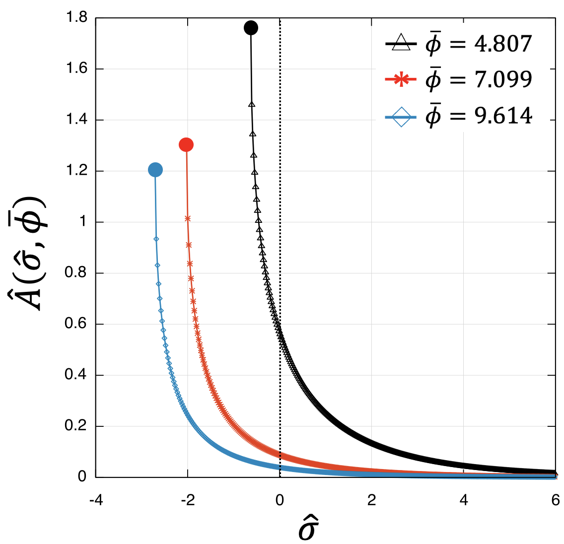
In Fig. 1, we plot the cage size with respect to the particle size for several packing fractions. The triangles represent the cage size at the dynamic glass transition density . The cage size is finite only in . This means that larger particles with are trapped in the cage and behave as a glass, while smaller particles with behave as a liquid. This dynamic decoupling is mentioned in the Introduction. We define the critical particle size , above which the cage size is finite. At this density , the critical particle size is .
The asterisks and squares in Fig. 1 represent the cage sizes at two higher densities. Increasing the density decreases the cage size and the critical particle size , thus causing the vitrification of smaller particles.
III.2 Asymptotic analysis
In this subsection, we analyze the self-consistent equations Eqs. (15) and (16) semianalytically. In particular, we derive several asymptotic laws of cage size in the NM system.
III.2.1 Large particles:
First, we focus on large particles with . Fig. 1 shows that the cage size rapidly decreases with in this regime. We derive an asymptotic law of this behavior.
In Eq. (15), the argument of the function is the average of the two cage sizes: . We now assume , so that the average can be approximated by . Under this condition, the function is independent of , and Eq. (15) is reduced to
| (17) |
This means that the cage size decreases exponentially with the particle size. Because this verifies the assumption at , the exponential law Eq. (17) is valid at .
III.2.2 In the vicinity of the critical size:
Next, we focus on the particles with size close to the critical size, . Fig. 1 shows that the cage size drastically decreases with a slight increase in . We analyze this behavior.
Following the anlaysis for the monodisperse system [25], we first transform Eq. (16) into the following form:
| (18) |
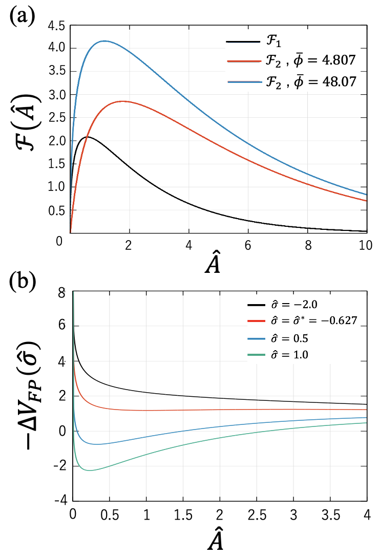
where we introduce an auxiliary function . According to Eq. (18), the intersection of and the horizontal line determines . Because the function has only one maximum (see Fig. 3a), the dynamic glass transition density is determined by .
We consider a similar transformation of Eq. (15). When we fix the packing fraction at , we can treat as a finite constant. Therefore, Eq. (15) can be transformed into
| (19) |
where we introduce an auxiliary function . As shown in Fig. 3a, this auxiliary function behaves quite similarly to . The intersection of and the horizontal line determines the cage size for any . Accordingly, the critical particle size is determined by
| (20) |
Now, we focus on the vicinity of the critical size. By introducing a simplified notation , we expand the particle size as and the cage size as . Substituting these into Eq. (19) and expanding both sides, we obtain
| (21) |
in the lowest orders of and . The prime symbol indicates the derivative of with respect to . Because corresponds to the maximum of , the first derivative vanishes and the second derivative is negative . Therefore, we obtain , or equivalently,
| (22) |
Because this argument is independent of the density, Eq. (22) should be valid in any .
The square-root singularity shown in Eq. (22) indicates that -sized particles are on the verge of spinodal instability. To discuss this point directly, we investigated the FP potential. By substituting Eq. (14) into Eq. (11), we obtain the FP potential of the NM system. In the leading order of , this FP potential can be decomposed into the contribution from each particle size. With the omission of unimportant constants, the contribution from is
| (23) |
where 111 Note that we can reproduce the self-consistent equation Eq. (15) by imposing the stationary point condition on Eq. (23).. In Fig. 3b, we plot for four representative particle sizes at the density . has a stationary point for larger particles but not for smaller particles . At the critical size , a stationary point emerges at which the FP potential becomes flat. This clearly shows that -sized particles are on the verge of spinodal instability. For monodisperse systems, the same instability is known to emerge at the dynamic glass transition density . By contrast, for the NM system, this instability is ubiquitous at since there are always -sized particles in the system.
III.2.3 Density dependence
Finally, we analyze the density dependence of the cage size in the vicinity of the dynamic glass transition, . To this end, we expand the density as . Furthermore, we expand the cage size as and , introducing simplified notations and . By substituting these expressions into Eqs. (18) and (19) and expanding them, we can obtain the critical law in the vicinity of the dynamic glass transition.
We first focus on , where the argument is precisely the same as in the monodisperse case. In this case, we can expand Eq. (18) as
| (24) |
in the leading order of and . Therefore, we obtain .
We then focus on . In this case, we need to calculate the variation in in both and . This can be done by observing
| (25) |
Expanding Eq. (III.2.3) in and and substituting it into Eq. (19), we obtain
| (26) |
for the relevant terms. In this equation, the lowest order of is not found on the left-hand side, but instead is the third term on the right-hand side because . The first term and the third term on the right-hand side should be balanced, which results in . However, if , the first term vanishes as discussed in the previous subsection. Thus, in this case, the second and the third terms on the right-hand side should be balanced, which results in . Summarizing these results, we obtain the following critical law for the density dependence of the cage size:
| (27) |
in the vicinity of the dynamic glass transition. Interestingly, the density dependence is modified for -sized particles, which is due to the coexistence of two criticalities associated with the dynamic glass transition density and the critical particle size.
III.2.4 Summary
We summarize the results of the asymptotic analysis for the NM system. At a fixed density, the cage size decreases exponentially with the particle size at (Eq. (17)) and decreases in the power law with the exponent at (Eq. (22)). This square-root singularity originates from spinodal instability of -sized particles, as depicted in Fig. 3b. When the density is varied, the cage size decreases with the density in the power-law with the exponent for -sized particles and for other particles (Eq. (27)).
IV Exponential distribution system
The NM system studied in the previous section is characterized by an extremely narrow particle size distribution. In this section, we focus on a more polydisperse system. Specifically, we study exponential distribution (ED) systems in which the particle size follows an exponential distribution:
| (28) |
Here, represents the upper cutoff of the particle size, and is a parameter related to the width of the distribution. At smaller , the distribution becomes broader, and the system becomes more polydisperse. We refer to as the width parameter. The normalization constant satisfies . In the following, we mainly study the case of and discuss -dependence later.
IV.1 Interpretation in the finite dimensions
First, we argue that the ED system is an infinite-dimensional counterpart of the power-law distribution systems in finite dimensions. To this end, we consider a continuously polydisperse system in the -dimension, where the particle size follows the distribution:
| (29) |
This distribution appears frequently in nature. For example, in foams [40], grains in rocks, and sediments formed by an impact fracture [41, 42, 43], the particle size distribution is often described by Eq. (29). Additionally, in recent simulation studies on the glass transition, Eq. (29) has been frequently adopted to accelerate numerical simulations [10].
Substituting the particle size scaling Eq. (2) into Eq. (29) and taking while keeping constant, we obtain
| (30) |
Therefore, the exponential distribution Eq. (28) is the infinite-dimensional counterpart of the power-law distribution Eq. (29), where the width parameter is given by .
IV.2 Numerical Results
Substituting the exponential distribution Eq. (28) into the self-consistent equation Eq. (12), we obtain the integral equation for the cage size . We solved this equation numerically via an iterative method. We first show the results for two representative cases: and .
IV.2.1 Narrow distribution:
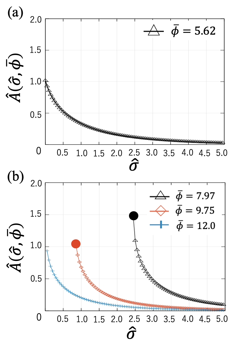
We solved the self-consistent equation for at various densities. We found that the cage size becomes finite at ; therefore, the dynamic glass transition density is . Fig. 4a shows the cage size at the dynamic glass transition density. The cage size is finite in the entire domain of the particle size: . This means that all the particles in the system simultaneously vitrified.
IV.2.2 Broad distribution:
Next, we solved the self-consistent equation for at various densities. We found that the cage size becomes finite only at . Fig. 4b shows the cage size at several densities. At the dynamic glass transition density, the cage size is finite for large particles, but not for small particles. Therefore, dynamic decoupling occurs. Following the analysis for the NM system, we define the critical particle size above which the cage size is finite. We emphasize that differs from the lower cutoff and the upper cutoff of the particle size distribution. In other words, when the system vitrifies, the system spontaneously defines the “larger” particles via the self-consistent equation.
At higher densities, the cage size decreases, and the critical particle size also decreases. At , the critical particle size vanishes , meaning that all the particles vitrify at this density. We define the complete dynamic glass transition density as the density above which the cage size is finite in the entire domain of the particle size. The complete dynamic glass transition density is .
IV.2.3 Phase diagram
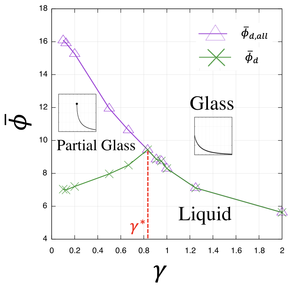
We repeated the cage size calculations at various and . We summarize the results in Fig. 5 as a phase diagram. The green crosses and the purple triangles show the dynamic glass transition density and the complete dynamic glass transition density , respectively. For any , the system is in a liquid state at low densities, while the cage size becomes finite, and the system vitrifies at high densities. When is large (cf. ), the dynamic glass transition density coincides with the complete dynamic glass transition density . Namely, the cage sizes for all the particles become finite simultaneously. On the other hand, when is small (cf. ), we find . Namely, larger particles vitrify first, and smaller particles vitrify only at higher densities. We refer to the state at as “glass”, where all the particles vitrify, and the state at as “partial glass”, where only larger particles vitrify. The two glass transition lines merge at , which we call the critical width parameter. The partial glass phase appears only when the size distribution is sufficiently broad, .
IV.3 Asymptotic Analysis
In Sec. III, we derived several asymptotic laws of the cage size in the NM system. Here, we discuss the validity of these laws in the ED system. The semianalytical approach for the NM system cannot be applied to the ED system because is coupled with all other via the self-consistent equation Eq. (12). However, we show that the cage size of the ED system still follows the same asymptotic laws, suggesting that the understanding of the NM system is effective even for the ED system.
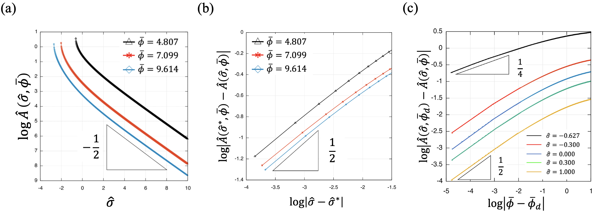
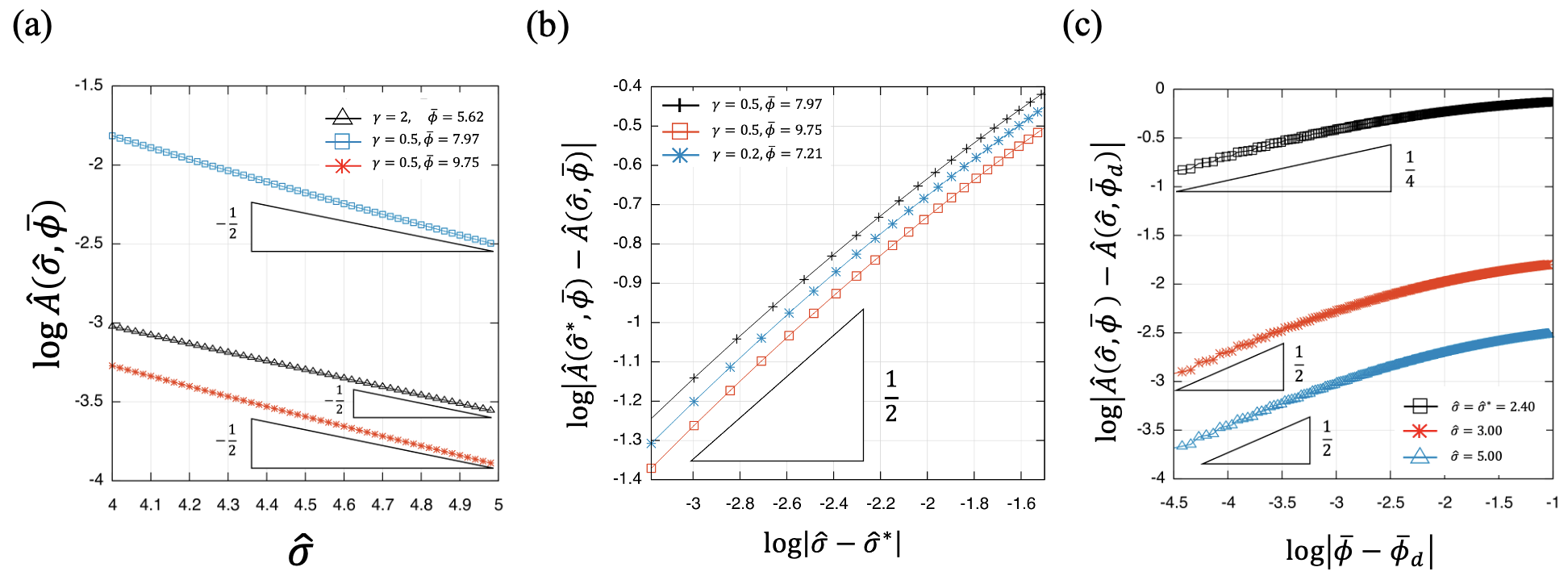
First, we focus on the cage size of large particles. In the NM system, the cage size decreases exponentially with increasing particle size, as Eq. (17). To verify this exponential law in the ED system, we plotted the logarithm of the cage size with respect to the particle size in Fig. 6a. For the state (, ) in the Glass phase, the slope works well, suggesting the validity of the exponential law. However, the description by the exponential law becomes slightly worse for (, ) and worse for (, ) in the partial glass phase. This deviation occurs because the focused particle size is not far from the critical particle size in these states, and the results suffer from the square-root singularity associated with . Therefore, we conclude that the exponential law Eq. (17) is valid for as long as .
Next, we focus on the vicinity of the critical particle size, . In the NM system, the cage size exhibits the square-root singularity shown in Eq. (22), which originates from the spinodal instability at . To verify the square-root singularity in the ED system, we plotted with respect to in Fig. 6b. The data are for several state points in the partial glass phase, where the critical particle size is finite. Clearly, all the data are consistent with the slope , and thus, the square-root singularity Eq. (22) is valid even in the ED system.
Finally, we focus on the density dependence of the cage size. In the NM system, the cage size follows the critical laws Eq. (27): the power-laws with exponents for and for . To verify this in the ED system, we plotted with respect to in Fig. 6c. Clearly, the slope is for and for . Therefore, the critical laws of Eq. (27) are valid even in the ED system.
In summary, all the critical laws derived for the NM system are valid in the ED system. The validity of the square-root singularity Eq. (22) suggests that -sized particles are on the verge of spinodal instability (see Fig. 3b), even in the ED system. Because there are always -sized particles in the system in the partial glass phase, this instability is ubiquitous in this phase, which is in sharp contrast to the monodisperse system.
IV.4 Cutoff dependence
Thus far, we have studied the ED system with the fixed cutoff . Here, we discuss the -dependence of the results. The system is now characterized by three parameters: the packing fraction , the width parameter , and the cutoff particle size . We solved the self-consistent equation for several states (, , ) and found that the critical laws are valid for all studied. Thus, we discuss the -dependence of the phase diagram, mainly focusing on the partial glass phase.
To this end, we focus on -dependence of the critical width parameter because it controls the presence and location of the partial glass phase. We found that decreases with decreasing , and becomes at . This means that the partial glass phase is absent when . This tendency is natural because the system approaches the monodisperse system in . On the other hand, we found that increases with increasing , and asymptotically approaches in : for and for . As a result, the phase diagram for larger is qualitatively similar to Fig. 5 with .
V Summary and Discussion
In this work, we developed a replica theory of hardspheres with continuous polydispersity in infinite spatial dimensions . We focused on the dynamic glass transition, for which the replica symmetric solution suffices. We first constructed an equilibrium liquid theory and then extended it to the liquids of replica molecules for continuously polydisperse systems. By this, we derived the FP potential, an effective free energy describing the glass transition. In contrast to the monodisperse systems, the cage size , the order parameter, depends on the particle size as , and thus, the FP potential is a functional of . By imposing a stationary point condition, we derived a self-consistent equation for the cage size, Eq. (12).
We first solved Eq. (12) for the nearly monodisperse (NM) system. The NM system is characterized by a narrow particle size distribution, where a semianalytical solution of Eq. (12) is available. We found that the critical particle size emerges and that dynamic decoupling occurs; larger particles vitrify, while smaller particles remain in a liquid state. In the vicinity of the critical particle size, the cage size exhibits the square-root singularity shown in Eq. (22), which originates from spinodal instability of -sized particles as illustrated in Fig. 3b.
We next solved Eq. (12) for the exponential distribution (ED) system, which is characterized by more realistic, broader particle size distributions. As shown in Fig. 5, this system has three phases: the liquid, glass, and partial glass phases. In the partial glass phase, the critical particle size emerges, dynamic decoupling occurs, and the cage size exhibits a square-root singularity at , as in the NM system. This means that at any density in the partial glass phase, there are always -sized particles in the system, which are on the verge of spinodal instability. This is in sharp contrast to the monodisperse system, for which spinodal instability occurs only at the dynamic glass transition density.
We now compare our results with those of previous works on finite-dimensional systems. Shimamoto et al. [40] numerically and experimentally studied the jamming transition of continuously polydisperse particles with in two-dimensions . Interestingly, their jamming phase diagram is quite similar to Fig. 5, the phase diagram of the ED system. They found that the fluid density is maximized at and that many particles become rattlers in the jammed phase at . Although they studied not the glass transition but the jamming transition, their results are qualitatively similar to our results in that the liquid density is maximized at and the partial glass phase appears at . We can quantitatively compare with because the width parameter and the exponent are related as (see Section IV A). Our result implies , which is not far from their observation . Extending our theory for the jamming transition would be interesting for a more direct comparison.
The glass transition of power-law distribution systems with has been actively studied in simulations, where the standard choice is in . Using this system, Pihlajamaa et al. [21] recently reported that larger particles are caged well while some fraction of smaller particles remain mobile. This observation is qualitatively similar to the phenomenology of the partial glass phase in the ED system. As we noted, our result implies that the partial glass phase emerges for . It would be interesting to systematically study the glass transition for in simulations, which will provide more information on the partial glass phase.
Finally, we mention two additional research directions to extend our work. First, it is interesting to study the Gardner transition of continuously polydisperse hardspheres. As we showed, this system has a partial glass phase, in which -sized particles are on the verge of spinodal instability. It is highly nontrivial how the Gardner transition occurs by compressing such partial glasses. It is also interesting to extend our theory to finite-dimensional systems by combining replica liquid theory with finite-dimensional liquid state theory. This should enable us to compare the theory with simulations and experiments more quantitatively.
Acknowledgements.
We thank H. Ikeda, Y. Tomita, H. Mizuno, F. Ghimenti, and F. van Wijland for insightful discussions and useful exchanges. This work was supported by JSPS KAKENHI Grant Numbers JP20H01868 and JP20H00128.References
- Bareigts et al. [2020] G. Bareigts, P.-C. Kiatkirakajorn, J. Li, R. Botet, M. Sztucki, B. Cabane, L. Goehring, and C. Labbez, Packing polydisperse colloids into crystals: When charge-dispersity matters, Phys. Rev. Lett. 124, 058003 (2020).
- Sollich [2001] P. Sollich, Predicting phase equilibria in polydisperse systems, Journal of Physics: Condensed Matter 14, R79 (2001).
- Auer and Frenkel [2001] S. Auer and D. Frenkel, Suppression of crystal nucleation in polydisperse colloids due to increase of the surface free energy, Nature 413, 711 (2001).
- Schöpe et al. [2006] H. J. Schöpe, G. Bryant, and W. van Megen, Small changes in particle-size distribution dramatically delay and enhance nucleation in hard sphere colloidal suspensions, Phys. Rev. E 74, 060401 (2006).
- Pusey and van Megen [1986] P. N. Pusey and W. van Megen, Phase behaviour of concentrated suspensions of nearly hard colloidal spheres, Nature 320, 340 (1986).
- Debenedetti [1996] P. Debenedetti, Metastable Liquids: Concepts and Principles, Physical Chemistry: Science and Engineering (Princeton University Press, 1996).
- Brambilla et al. [2009] G. Brambilla, D. El Masri, M. Pierno, L. Berthier, L. Cipelletti, G. Petekidis, and A. B. Schofield, Probing the equilibrium dynamics of colloidal hard spheres above the mode-coupling glass transition, Phys. Rev. Lett. 102, 085703 (2009).
- Bernu et al. [1987] B. Bernu, J. P. Hansen, Y. Hiwatari, and G. Pastore, Soft-sphere model for the glass transition in binary alloys: Pair structure and self-diffusion, Phys. Rev. A 36, 4891 (1987).
- Kob and Andersen [1995] W. Kob and H. C. Andersen, Testing mode-coupling theory for a supercooled binary lennard-jones mixture i: The van hove correlation function, Phys. Rev. E 51, 4626 (1995).
- Ninarello et al. [2017] A. Ninarello, L. Berthier, and D. Coslovich, Models and algorithms for the next generation of glass transition studies, Phys. Rev. X 7, 021039 (2017).
- Henderson et al. [1996] S. Henderson, T. Mortensen, S. Underwood, and W. van Megen, Effect of particle size distribution on crystallisation and the glass transition of hard sphere colloids, Physica A: Statistical Mechanics and its Applications 233, 102 (1996).
- Zaccarelli et al. [2009] E. Zaccarelli, C. Valeriani, E. Sanz, W. C. K. Poon, M. E. Cates, and P. N. Pusey, Crystallization of hard-sphere glasses, Phys. Rev. Lett. 103, 135704 (2009).
- Behera et al. [2017] S. K. Behera, D. Saha, P. Gadige, and R. Bandyopadhyay, Effects of polydispersity on the glass transition dynamics of aqueous suspensions of soft spherical colloidal particles, Phys. Rev. Mater. 1, 055603 (2017).
- Zaccarelli et al. [2015] E. Zaccarelli, S. M. Liddle, and W. C. K. Poon, On polydispersity and the hard sphere glass transition, Soft Matter 11, 324 (2015).
- Imhof and Dhont [1995] A. Imhof and J. K. G. Dhont, Experimental phase diagram of a binary colloidal hard-sphere mixture with a large size ratio, Phys. Rev. Lett. 75, 1662 (1995).
- Hendricks et al. [2015] J. Hendricks, R. Capellmann, A. B. Schofield, S. U. Egelhaaf, and M. Laurati, Different mechanisms for dynamical arrest in largely asymmetric binary mixtures, Phys. Rev. E 91, 032308 (2015).
- Heckendorf et al. [2017] D. Heckendorf, K. J. Mutch, S. U. Egelhaaf, and M. Laurati, Size-dependent localization in polydisperse colloidal glasses, Phys. Rev. Lett. 119, 048003 (2017).
- Moreno and Colmenero [2006] A. J. Moreno and J. Colmenero, Relaxation scenarios in a mixture of large and small spheres: Dependence on the size disparity, The Journal of Chemical Physics 125, 164507 (2006).
- Voigtmann and Horbach [2009] T. Voigtmann and J. Horbach, Double transition scenario for anomalous diffusion in glass-forming mixtures, Phys. Rev. Lett. 103, 205901 (2009).
- Vaibhav et al. [2022] V. Vaibhav, J. Horbach, and P. Chaudhuri, Finite-size effects in the diffusion dynamics of a glass-forming binary mixture with large size ratio, The Journal of Chemical Physics 156, 244501 (2022).
- Pihlajamaa et al. [2023] I. Pihlajamaa, C. C. L. Laudicina, and L. M. C. Janssen, Influence of polydispersity on the relaxation mechanisms of glassy liquids, Phys. Rev. Res. 5, 033120 (2023).
- Parisi et al. [2020] G. Parisi, P. Urbani, and F. Zamponi, Theory of Simple Glasses: Exact Solutions in Infinite Dimensions (Cambridge University Press, 2020).
- Götze [2009] W. Götze, Complex Dynamics of Glass-Forming Liquids: A Mode-Coupling Theory, International Series of Monographs on Physics (OUP Oxford, 2009).
- Mézard and Parisi [1999] M. Mézard and G. Parisi, A first-principle computation of the thermodynamics of glasses, The Journal of Chemical Physics 111, 1076 (1999).
- Parisi and Zamponi [2010] G. Parisi and F. Zamponi, Mean-field theory of hard sphere glasses and jamming, Rev. Mod. Phys. 82, 789 (2010).
- Coluzzi et al. [1999] B. Coluzzi, M. Mézard, G. Parisi, and P. Verrocchio, Thermodynamics of binary mixture glasses, The Journal of Chemical Physics 111, 9039 (1999).
- Biazzo et al. [2009] I. Biazzo, F. Caltagirone, G. Parisi, and F. Zamponi, Theory of amorphous packings of binary mixtures of hard spheres, Phys. Rev. Lett. 102, 195701 (2009).
- Ikeda et al. [2016] H. Ikeda, K. Miyazaki, and A. Ikeda, Note: A replica liquid theory of binary mixtures, The Journal of Chemical Physics 145, 216101 (2016).
- Ikeda et al. [2017] H. Ikeda, F. Zamponi, and A. Ikeda, Mean field theory of the swap Monte Carlo algorithm, The Journal of Chemical Physics 147, 234506 (2017).
- Ikeda and Zamponi [2019] H. Ikeda and F. Zamponi, Effect of particle exchange on the glass transition of binary hard spheres, Journal of Statistical Mechanics: Theory and Experiment 2019, 054001 (2019).
- Ikeda et al. [2021] H. Ikeda, K. Miyazaki, H. Yoshino, and A. Ikeda, Multiple glass transitions and higher-order replica symmetry breaking of binary mixtures, Phys. Rev. E 103, 022613 (2021).
- Bosse and Kaneko [1995] J. Bosse and Y. Kaneko, Self-diffusion in supercooled binary liquids, Phys. Rev. Lett. 74, 4023 (1995).
- Voigtmann [2011] T. Voigtmann, Multiple glasses in asymmetric binary hard spheres, Europhysics Letters 96, 36006 (2011).
- Laudicina et al. [2023] C. C. L. Laudicina, I. Pihlajamaa, and L. M. C. Janssen, Competing relaxation channels in continuously polydisperse fluids: A mode-coupling study, Phys. Rev. Res. 5, 033121 (2023).
- Ikeda and Miyazaki [2010] A. Ikeda and K. Miyazaki, Mode-coupling theory as a mean-field description of the glass transition, Phys. Rev. Lett. 104, 255704 (2010).
- Wilding and Sollich [2002] N. B. Wilding and P. Sollich, Grand canonical ensemble simulation studies of polydisperse fluids, The Journal of Chemical Physics 116, 7116 (2002).
- Morita and Hiroike [1961] T. Morita and K. Hiroike, A New Approach to the Theory of Classical Fluids. III: General Treatment of Classical Systems, Progress of Theoretical Physics 25, 537 (1961).
- Stell [1964] G. Stell, Cluster expansions for classical systems in equilibrium., in The Equilibrium Theory of Classical Fluids, edited by H. Frisch and J. Lebowitz (Benjamin, New York, 1964) p. 171–261.
- Note [1] Note that we can reproduce the self-consistent equation Eq. (15) by imposing the stationary point condition on Eq. (23).
- Shimamoto and Yanagisawa [2023] D. S. Shimamoto and M. Yanagisawa, Common packing patterns for jammed particles of different power size distributions, Phys. Rev. Research 5, L012014 (2023).
- Sammis and King [2007] C. G. Sammis and G. C. P. King, Mechanical origin of power law scaling in fault zone rock, Geophysical Research Letters 34 (4), L04312 (2007).
- Oddershede et al. [1993] L. Oddershede, P. Dimon, and J. Bohr, Self-organized criticality in fragmenting, Phys. Rev. Lett. 71, 3107 (1993).
- Grott et al. [2020] M. Grott, J. Biele, P. Michel, S. Sugita, S. Schröder, N. Sakatani, W. Neumann, S. Kameda, T. Michikami, , and C. Honda, Macroporosity and grain density of rubble pile asteroid (162173) ryugu, J. Geophys. Res. Planets 125, e2020JE006519 (2020).