Non-unique Hamiltonians for Discrete Symplectic Dynamics

Abstract

An outstanding property of any Hamiltonian system is the symplecticity of its flow, namely, the continuous trajectory preserves volume in phase space. Given a symplectic but discrete trajectory generated by a transition matrix applied at a fixed time-increment ($\tau>0$), it was generally believed that there exists a unique Hamiltonian producing a continuous trajectory that coincides at all discrete times ($t=n\tau$ with $n$ integers) as long as $\tau$ is small enough. However, it is now exactly demonstrated that, for any given discrete symplectic dynamics of a harmonic oscillator, there exists an infinite number of real-valued Hamiltonians for any small value of $\tau$ and an infinite number of complex-valued Hamiltonians for any large value of $\tau$. In addition, when the transition matrix is similar to a Jordan normal form with the supradiagonal element of $1$ and the two identical diagonal elements of either $1$ or $-1$, only one solution to the Hamiltonian is found for the case with the diagonal elements of $1$, but no solution can be found for the other case.

Symplectic integratorsDe Vogelaere (1956); Ruth (1983); Feng (1985); Feng and Qin (1987) are widely used to simulate the dynamic processes of elementary particles, materials and celestial bodiesYoshida (1990); Frenkel and Smit (2023). In order to understand the structure, regularity and stability of the discrete dynamics generated by these integrators, it may be worth analyzing the motion in a Hamiltonian representation, just as it is realized in classical mechanicsArnold (1989). Despite recent progressGriffiths and Sanz-Serna (1986); Auerbach and Friedman (1991); Yoshida (1993); Toxvaerd (1994); Hairer (1994); Chin and Scuro (2005); Toxvaerd et al. (2012); Hammonds and Heyes (2020), the basic problems about the uniqueness and existence of this representation have not been solved for any model system.

When the classical system described by an original Hamiltonian, ${\cal H}_{0}(q,p)$, is propagated at a fixed time-increment $\tau$:

$$\begin{bmatrix}q((n+1)\tau)\\ p((n+1)\tau)\end{bmatrix}=\hat{R}\begin{bmatrix}q(n\tau)\\ p(n\tau)\end{bmatrix},$$ (1)

with $n=0,1,2,\cdots$ an integer and $\hat{R}$ a symplectic transition matrix derived from ${\cal H}_{0}(q,p)$, it is generally believed that there exists a slightly perturbed Hamiltonian ${\cal H}(\tau,q,p)$, also called shadow Hamiltonian by Toxvaerd et al.Toxvaerd (1994); Toxvaerd et al. (2012), such that the discrete phase points, $(q(n\tau),p(n\tau))$, lie on the continuous trajectory produced by the Hamilton’s canonical equations of motion,

$$\left\{\begin{aligned} \frac{dq(t)}{dt}\equiv\dot{q}&=\dfrac{\partial{\cal H}}{\partial p}\\ \frac{dp(t)}{dt}\equiv\dot{p}&=-\dfrac{\partial{\cal H}}{\partial q}\end{aligned}\right..$$ (2)

${\cal H}(\tau,q,p)$ was previously expressed by a formal power series in $\tau$ (e.g. Eq. (45) of ref.Yoshida (1993)):

$${\cal H}(\tau,q,p)={\cal H}_{0}(q,p)+\tau{\cal H}_{1}(q,p)+\tau^{2}{\cal H}_{2}(q,p)+\cdots.$$ (3)

When $\tau$ approaches $0$, ${\cal H}(\tau,q,p)$ necessarily reduces to ${\cal H}_{0}(q,p)$ up to a trivial additive constant independent of $q$ and $p$. Higher order corrections are uniquely formulated in terms of the Baker-Campbell-Hausdorff (BCH) expansionVaradarajan (1984) for the product of exponential operators involved in $\hat{R}$Dragt and Finn (1976); Dragt et al. (1988); Yoshida (1993). In this work, we instead solve exactly the system of one harmonic oscillator to explicitly demonstrate that, contrary to the assumed uniqueness, ${\cal H}(\tau,q,p)$ is in fact non-unique even for small $\tau$.

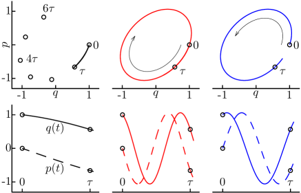
Figure 1: Typical continuous trajectories from $(q(0)=1,p(0)=0)$ to $(q(1.05\tau),p(1.05\tau))$ in the $qp$ phase space (top) and as functions of time (bottom, solid lines for $q(t)$ and dashed $p(t)$) generated by the Hamiltonians of Eq. (5) at $m=0$ (left), $1$ (middle, red) and $-1$ (right, blue). In the phase space, the trajectory of the phase points rotates clockwise ($m\geqslant 0$) and counter-clockwise ($m<0$) respectively. Discrete points: $q(n\tau)$ and $p(n\tau)$ at $n=0,1,2,\cdots,6$ (circles), are generated by the symplectic integrator. See Eq. (21).

For the system of the one-dimensional (1D) single harmonic oscillator defined by ${\cal H}_{0}=q^{2}/2+p^{2}/2$ in reduced units, the non-singular $2$ by $2$ transition matrix:

$$\hat{R}(\tau)=\begin{bmatrix}R_{1}(\tau)&R_{2}(\tau)\\ R_{3}(\tau)&R_{4}(\tau)\end{bmatrix},$$ (4)

depends on none of $n$, $q$ and $p$; it is only a function of the time-increment $\tau$. The symplectic condition requires that the determinant of $\hat{R}$ is unity: $R_{1}R_{4}-R_{2}R_{3}=1$, so the product of its two eigenvalues is $1$. Therefore, we denote the eigenvalues as $y$ and $1/y$, where $y$ is a complex number expressed in the exponential form: $y=\left|y\right|e^{i\theta}$ with $-\pi<\theta\leqslant\pi$. Possible solutions to ${\cal H}(\tau,q,p)$, which are independent of time or $n$, are listed in the following three categories.

i) When $(R_{1}+R_{4})^{2}\neq 4$, $\hat{R}$ has two distinct eigenvalues: $y\neq 1/y$, and ${\cal H}$ takes a binomial form:

$${\cal H}(\tau,q,p|m)=\frac{\log(y,m)}{\left(y-1/y\right)}\frac{R_{2}p^{2}-R_{3}q^{2}+(R_{1}-R_{4})pq}{\tau},$$ (5)

where the multivalued logarithm function is defined as

$$\log(y,m)=\log\left|y\right|+i\theta+i2m\pi,$$ (6)

with $m$ an arbitrary integer and $i$ the imaginary unit. i-a) When $\theta\neq 0$ and $\theta\neq\pi$, which is often the case for small $\tau$ in the traditional symplectic integratorsYoshida (1990); Frenkel and Smit (2023), the two distinct eigenvalues are complex conjugated: $1/y=y^{*}$ and the module must be $1$: $\left|y\right|^{2}=yy^{*}=1$. Both $\log(y,m)$ and $y-1/y$ give pure imaginary numbers and consequently ${\cal H}(\tau,q,p|m)$ are all real-valued. Specifically, ${\cal H}(\tau,q,p|0)$ reduces to the power series of Eq. (3) applied to the harmonic oscillator. Typical trajectories in the phase space and as functions of time for $m=0,\pm 1$ are shown in Fig. 1. i-b) When $\theta=0$, the two distinct eigenvalues are both positive: $y>0$, and then ${\cal H}(\tau,q,p|0)$ is still real-valued and other solutions with $m\neq 0$ all complex. i-c) When $\theta=\pi$, which is often the case for large $\tau$, the two distinct eigenvalues are both negative: $y<0$, and then no real-valued ${\cal H}(\tau,q,p|m)$ exists.

ii) When $\hat{R}=\pm\hat{I}$ with $\hat{I}$ the $2$ by $2$ identity matrix, $y=1/y=\pm 1$ and then ${\cal H}$ exists:

$${\cal H}(\tau,q,p|m)=i\pi\frac{4m+1\mp 1}{2}\frac{C_{2}p^{2}-C_{3}q^{2}+2C_{1}pq}{2\tau},$$ (7)

with $C_{1}$, $C_{2}$ and $C_{3}$ arbitrary complex numbers satisfying $C_{1}^{2}+C_{2}C_{3}=1$. There are an infinite number of real-valued and complex-valued Hamiltonians.

iii) When $y=1/y=\pm 1$ and $\hat{R}$ is similar to a Jordan normal form with the supradiagonal element of $1$ and the diagonal elements of $\pm 1$:

$$\hat{R}=\hat{P}\begin{bmatrix}\pm 1&1\\ 0&\pm 1\end{bmatrix}\hat{P}^{-1},$$ (8)

with $\hat{P}$ non-singular and $\hat{P}\hat{P}^{-1}=\hat{I}$, there must be $R_{1}+R_{4}=\pm 2$ but $\hat{R}\neq\pm\hat{I}$. A unique or no solution to ${\cal H}$ is found respectively. iii-a) When $y=1/y=1$ and $\hat{R}\neq\hat{I}$, the unique solution is

$${\cal H}(\tau,q,p)=\frac{R_{2}p^{2}-R_{3}q^{2}+2(R_{1}-1)pq}{2\tau}.$$ (9)

iii-b) When $y=1/y=-1$ and $\hat{R}\neq-\hat{I}$, no solution to ${\cal H}$ can be found.

Derivation. Obviously, the phase point that coincides with Eq. (1) at any discrete time could evolve continuously according to

$$\begin{bmatrix}q(t)\\ p(t)\end{bmatrix}={\hat{R}}^{t/\tau}\begin{bmatrix}q(0)\\ p(0)\end{bmatrix}=\exp\left(\dfrac{t}{\tau}\hat{Z}\right)\begin{bmatrix}q(0)\\ p(0)\end{bmatrix},$$ (10)

where the matrix $\hat{Z}$ is determined by the matrix equation,

$$e^{\hat{Z}}=\hat{R},$$ (11)

with the exponential interpreted as a Taylor series:

$$e^{\hat{Z}}=\hat{I}+\hat{Z}+\frac{1}{2}\hat{Z}^{2}+\cdots+\frac{1}{k!}\hat{Z}^{k}+\cdots.$$ (12)

For any known $\hat{R}$, all the solutions of Eq. (11) are called (natural) logarithm of $\hat{R}$ (p. 239 of ref.Gantmacher (1959)). The eigenvalues $x_{j}$ of $\hat{Z}$ are connected with the eigenvalues $y_{j}$ of $\hat{R}$ by the formula: $y_{j}=e^{x_{j}}$, thus, $y_{j}$ must be non-zero, i.e., $\hat{R}$ is non-singular, such that $x_{j}$ exists. In addition, the Hamilton-Cayley theorem states that any matrix satisfies its own characteristic equation (p.83 of ref.Gantmacher (1959)):

$$\left(Z_{1}\hat{I}-\hat{Z}\right)\left(Z_{4}\hat{I}-\hat{Z}\right)-Z_{2}Z_{3}\hat{I}=0.$$ (13)

This theorem simplifies all higher order multiplications in the Taylor series of Eq. (12) to linear combinations of $\hat{Z}$ and $\hat{I}$ only. As a consequence, Eq. (11) implies a linear matrix equation with two coefficients, $a$ and $b$:

$$a\hat{Z}+b\hat{I}=\hat{R}.$$ (14)

The connection between the assumed continuous trajectory of Eq. (10) and the canonical equations of motion, Eq. (2), is made clear by taking the time derivative:

$$\left\{\begin{aligned} \dot{q}=\frac{Z_{1}q+Z_{2}p}{\tau}&=\dfrac{\partial{\cal H}}{\partial p}\\ \dot{p}=\frac{Z_{3}q+Z_{4}p}{\tau}&=-\dfrac{\partial{\cal H}}{\partial q}\end{aligned}\right..$$ (15)

Certainly, the elements of $\hat{Z}$ for the harmonic oscillator are only functions of $\tau$ for the reason that $\hat{R}$ is. For the partial derivatives being linearly dependent on $p$ and $q$, ${\cal H}$ must exist in a binomial form up to an additive constant:

$${\cal H}=\frac{Z_{2}p^{2}-Z_{3}q^{2}+2Z_{1}pq}{2\tau}=\frac{Z_{2}p^{2}-Z_{3}q^{2}-2Z_{4}pq}{2\tau},$$ (16)

if and only if $\hat{Z}$ satisfying Eq. (11) is traceless: $Z_{1}+Z_{4}=0$, or equivalently, the sum of the two eigenvalues of $\hat{Z}$ equals $0$: $x_{1}+x_{2}=0$. The symplectic condition imposed on $\hat{R}$: $R_{1}R_{4}-R_{2}R_{3}=y_{1}y_{2}=e^{x_{1}+x_{2}}=1$ becomes necessary, as expected. However, as demonstrated in the below, this condition is not sufficient to reach a traceless $\hat{Z}$ from Eq. (11).

By analyzing the elementary divisors (Jordan blocks) of $\hat{R}$ and then expressing $a$ and $b$ of Eq. (14) in terms of the elements and eigenvalues of $\hat{R}$, we derive ${\cal H}$ corresponding to the three categories in the preceding section.

i) When $y_{1}\neq y_{2}$, setting $y_{1}=y$ and $x_{1}=\log(y,m)=-x_{2}$ and then equating the eigenvalues of the matrices in Eq. (14) simply yield the coefficients $a$ and $b$. Consequently,

$$\hat{Z}=\frac{\log(y,m)}{y-1/y}\left(2\hat{R}-\frac{y^{2}+1}{y}\hat{I}\right),$$ (17)

which is indeed traceless on account of $y_{1}+y_{2}=(y^{2}+1)/y=R_{1}+R_{4}$. Hence, Eqs. (16) and (17) give the desired result, Eq. (5).

ii) When $y_{1}=y_{2}=y$ and $\hat{R}=y\hat{I}$, setting $x_{1}=\log(y,m)=-x_{2}$ again leads to $x_{1}=\log(y,m)=i\pi(4m+1\mp 1)/2$, in which $\mp$ corresponds to $y=\pm 1$, i.e., $\theta=0$ and $\theta=\pi$ in Eq. (6), respectively. Since $\hat{R}=y\hat{I}$ always produces $a=0$ and $b=y$ in Eq. (14) for any non-zero $\hat{Z}$, an arbitrary traceless $2$ by $2$ matrix with its two distinct eigenvalues: $i\pi(4m+1\mp 1)/2$ and $-i\pi(4m+1\mp 1)/2$ respectively, is always a valid solution to $\hat{Z}$. Hence, Eq. (7).

iii) When $y_{1}=y_{2}=y$ but $\hat{R}\neq y\hat{I}$, $\hat{R}$ must be similar to a Jordan normal form with the supradiagonal element of $1$, so does $\hat{Z}$. Because this non-diagonal Jordan form must imply $x_{1}=x_{2}$, the eigenvalues additionally subject to the constraint: $x_{1}=-x_{2}$, have to be both zero: $x_{1}=x_{2}=0$ and thus $y=e^{x_{1}}=1$. In this case, higher order multiplications in the Taylor series of Eq. (12) all vanish: $\hat{Z}^{k}=0$ for any $k=2,3,\cdots$, and only the first two terms survive to give $a=b=1$ in Eq. (14). Hence, $\hat{Z}=\hat{R}-\hat{I}$ and then Eq. (9). On the other hand, when $y_{1}=y_{2}=-1$ but $\hat{R}\neq-\hat{I}$, no traceless solution to $\hat{Z}$ can be found.

Examples and Discussions. The transition matrix for the symplectic Euler (E) integrator reads explicitlyYoshida (1993); Donnelly and Rogers (2005)

$$\hat{R}_{\rm E}(\tau)=\begin{bmatrix}R_{1}(\tau)&R_{2}(\tau)\\ R_{3}(\tau)&R_{4}(\tau)\end{bmatrix}=\begin{bmatrix}1-\tau^{2}&\tau\\ -\tau&1\end{bmatrix}.$$ (18)

According to iii-b), ${\cal H}$ does not exist when $\tau=2$; otherwise, there are an infinite number of valid Hamiltonians. When $0<\tau<2$, the explicit expression for ${\cal H}$ follows Eq. (5) and the category i-a)

$${\cal H}(\tau,q,p|m)=\lambda_{m}\frac{p^{2}+q^{2}-\tau pq}{\tau\sqrt{4-\tau^{2}}},$$ (19)

where $\lambda_{m}=2m\pi+{\rm acos}(1-\tau^{2}/2)$. Here, it is crucial to use ${\rm acos}(1-\tau^{2}/2)\in(0,\pi)$ rather than ${\rm asin}(\tau\sqrt{1-\tau^{2}/4})\in(0,\pi/2)$ for $0<\tau<2$. ${\cal H}(\tau,q,p|0)$ at $m=0$ with the smallest $\lvert\lambda_{m}\rvert$ identifies with the power series of Eq. (3) and the expression previously derived by Donnelly and RogersDonnelly and Rogers (2005); not .

Similarly, when $\tau>2$, Eq. (5) and i-c) yield the complex-valued time-independent Hamiltonians:

$${\cal H}(\tau,q,p|m)=\lambda_{m}\frac{p^{2}+q^{2}-\tau pq}{\tau\sqrt{\tau^{2}-4}},$$ (20)

where the complex number $\lambda_{m}=i(2m+1)\pi+\log 2-\log(\tau^{2}-2+\tau\sqrt{\tau^{2}-4})$. Somewhat surprisingly, the Hamilton’s equations of motion in the complex plane do represent the symplectic discrete dynamics in the real space! However, the power series of Eq. (3) yields no valid Hamiltonian any more because it diverges for $\tau>2$. Tracing back to the matrix $\hat{Z}$ in Eq. (11), it is important to keep its complex-valued solutions; obviously, these solutions can not be derived from the previous BCH technique (e.g.Yoshida (1993)), which at most leads to one real-valued expression. It should be possible to extend this technique to get multiple power series. Such an extension might be useful for solving other problems that have been dealt with by the BCH technique associated with Lie algebraVaradarajan (1984).

Setting $t_{m}=\lambda_{m}t/\tau$, the trajectory at a given initial condition: $q(0)=q_{0}$ and $p(0)=p_{0}$ reads correspondingly,

$$\left\{\begin{aligned} q(t)&=\left(2p_{0}-\tau q_{0}\right)\dfrac{\sin(t_{m})}{\sqrt{4-\tau^{2}}}+q_{0}\cos(t_{m})\\ p(t)&=\left(\tau p_{0}-2q_{0}\right)\dfrac{\sin(t_{m})}{\sqrt{4-\tau^{2}}}+p_{0}\cos(t_{m})\end{aligned}\right.$$ (21)

for $0<\tau<2$, and

$$\left\{\begin{aligned} q(t)&=\left(2p_{0}-\tau q_{0}\right)\dfrac{\sinh(t_{m})}{\sqrt{\tau^{2}-4}}+q_{0}\cosh(t_{m})\\ p(t)&=\left(\tau p_{0}-2q_{0}\right)\dfrac{\sinh(t_{m})}{\sqrt{\tau^{2}-4}}+p_{0}\cosh(t_{m})\end{aligned}\right.$$ (22)

for $\tau>2$, where the hyperbolic trigonometric functions $\sinh(x)=\left(e^{x}-e^{-x}\right)/2$ and $\cosh(x)=\left(e^{x}+e^{-x}\right)/2$. Eqs. (21) and (22) have the same structure; the only difference between them is whether the triangle functions or the hyperbolic trigonometric functions are used. It is easy to verify that both equations agree with the discrete dynamics described by Eq. (1) and (18). Clearly, the generalized momentum (velocity), $p$, is not the time derivative of the generalized coordinate, $q$, any more: $p\neq\dot{q}$, which is evident from the fact that the binomial forms in ${\cal H}(\tau,q,p|m)$ of Eqs. (19) and (20) include the nontrivial coefficients and the cross term of $pq$. Then it is necessary to derive more accurate expressions of velocities and related kinetic energy, rather than use the direct output of the integratorGans and Shalloway (2000); Toxvaerd (2024). Fig. 1 shows the first several trajectories obtained from Eq. (21) with $0<\tau=0.66<2$, $m=0,\pm 1$ and the initial state: $(q_{0}=1,p_{0}=0)$. In the $qp$ phase space, the trajectory rotates clockwise for any $m\geqslant 0$ and counter-clockwise for any $m<0$. Besides, the period dramatically decreases as $\left|m\right|$ and the real-valued $t_{m}$ increase when $0<\tau<2$. In contrast, when $\tau>2$, the hyperbolic trigonometric functions with the complex-valued $t_{m}$ as the input must result in divergent trajectories.

${\cal H}$ for the usual velocity-Verlet (v) or position-Verlet (p) integratorsTuckerman et al. (1992); Frenkel and Smit (2023) identically falls into the categories i-a), iii-b), and i-c) for $0<\tau<2$, $\tau=2$, and $\tau>2$ respectively. Because $R_{1}=R_{4}=1-\tau^{2}/2$ in the Verlet integrators, Eq. (5) produces the binomial form of ${\cal H}$ without the cross term of $pq$. However, the nontrivial coefficients different from $1/2$ in ${\cal H}_{0}(q,p)$ still exist and contribute to the Boltzmann distribution, $\propto e^{-\beta{\cal H}(q,p,\tau|m)}$, which might be sampled by symplectic integrators coupled with a thermostat. The coupling possibly follows the current schemesLeimkuhler and Matthews (2013); Li et al. (2017); the .

At some critical time-increment, typical symplectic integrators often suffer from the non-existence of ${\cal H}$ due to the non-diagonal Jordan form with eigenvalues $-1$. It is always possible to create new symplectic integrators to eliminate this singularity. For example, one might simply define a double Euler (dE) integrator as $\hat{R}_{\rm dE}(\tau)=\hat{R}_{\rm E}(\tau/2)\hat{R}_{\rm E}(\tau/2)$ such that its eigenvalues at the critical time-increment, $\tau/2=2$, change from $-1$ to $1$. ${\cal H}$ for $\hat{R}_{\rm dE}(\tau)$ falls into the categories i-a) for $0<\tau<2\sqrt{2}$ and $2\sqrt{2}<\tau<4$, ii) for $\tau=2\sqrt{2}$, iii-a) for $\tau=4$, and i-b) for $\tau>4$, respectively. However, a combination of two distinct integrators might still fail, just as $\hat{R}_{\rm vp}(\tau)=\hat{R}_{\rm v}(\tau/2)\hat{R}_{\rm p}(\tau/2)$ does. It is of course straightforward to analyze $\hat{R}_{\rm vp}(\tau)$ and any other time-independent transition matrix for the harmonic oscillator.

In a word, we have exactly solved the Hamiltonian representation of arbitrary discrete symplectic dynamics of the one-dimensional single harmonic oscillator. The representation illustrates the structure, regularity and stability of the discrete symplectic dynamics in a transparent way. At a small time-increment, the obtained time-independent Hamiltonian avoids the standard power series derived by the Baker-Campbell-Hausdorff (BCH) technique associated with Lie algebra and it is proved to be non-unique. At a large time-increment, the complex-valued Hamilton’s equations of motion surprisingly represent the discrete motion in the real space. It is also possible to solve linear systems of many harmonic oscillators in the three dimensions, because the derived transition matrices remain only functions of the time-increment. However, it is difficult to deal with any nonlinear system, because the elements of its transition matrix are in fact $q$- and $p$-dependent operators and the convergence of the power series has not been rigorously known even for a small time-incrementYoshida (1993).

References

- De Vogelaere (1956) R. De Vogelaere, “Methods of integration which preserve the contact transformation property of the hamilton equations,” Technical report (University of Notre Dame. Dept. of Mathematics) (1956).
- Ruth (1983) R. D. Ruth, “A canonical integration technique,” IEEE Trans. Nucl. Sci. 30, 2669–2671 (1983).
- Feng (1985) K. Feng, Proceedings of the 1984 Beijing Symposium on Differential Geometry and Differential Equations: Computation of Partial Differential Equations (Science Press, 1985).
- Feng and Qin (1987) K. Feng and M.-Z. Qin, Numerical methods for partial differential equations (Springer, 1987) pp. 1–37.
- Yoshida (1990) H. Yoshida, “Construction of higher order symplectic integrators,” Phys. Lett. A 150, 262–268 (1990).
- Frenkel and Smit (2023) Daan Frenkel and Berend Smit, Understanding Molecular Simulation: From Algorithms to Applications, 3rd ed. (Academic Press, Inc., San Diego, 2023).
- Arnold (1989) V. I. Arnold, Mathematical Methods of Classical Mechanics, 2nd ed. (Springer-Verlag, New York, 1989).
- Griffiths and Sanz-Serna (1986) D. F. Griffiths and J. M. Sanz-Serna, “On the scope of the method of modified equations,” SIAM J. Sci. Stat. Comput. 7, 994–1008 (1986).
- Auerbach and Friedman (1991) S. P. Auerbach and A. Friedman, “Long-time behaviour of numerically computed orbits: Small and intermediate timestep analysis of one-dimensional systems,” J. Comput. Phys. 93, 189–223 (1991).
- Yoshida (1993) H. Yoshida, “Recent progress in the theory and application of symplectic integrators,” Celest. Mech. Dyn. Astr. 56, 27–43 (1993).
- Toxvaerd (1994) S. Toxvaerd, “Hamiltonians for discrete dynamics,” Phys. Rev. E 50, 2271–2274 (1994).
- Hairer (1994) E. Hairer, “Backward analysis of numerical integrators and symplectic methods,” Ann. Numer. Math. 1, 107–132 (1994).
- Chin and Scuro (2005) S. A. Chin and S. R. Scuro, “Exact evolution of time-reversible symplectic integrators and their phase errors for the harmonic oscillator,” Phys. Lett. A 342, 397–403 (2005).
- Toxvaerd et al. (2012) S. Toxvaerd, O. J. Heilmann, and J. C. Dyre, “Energy conservation in molecular dynamics simulations of classical systems,” J. Chem. Phys. 136, 224106 (2012).
- Hammonds and Heyes (2020) K. D. Hammonds and D. M. Heyes, “Shadow hamiltonian in classical nve molecular dynamics simulations: A path to long time stability,” J. Chem. Phys. 152, 024114 (2020).
- Varadarajan (1984) V. S. Varadarajan, Lie groups, Lie algebras, and their representations (Springer, 1984).
- Dragt and Finn (1976) A. J. Dragt and J. M. Finn, “Lie series and invariant functions for analytic symplectic maps,” J. Math. Phys. 17, 2215–2227 (1976).
- Dragt et al. (1988) A. J. Dragt, F. Neri, G. Rangarajan, D. Douglas, L. M. Healy, and R. D. Ryne, “Lie algebraic treatment of linear and nonlinear beam dynamics,” Annu. Rev. Nucl. Part. S. 38 (1988).
- Gantmacher (1959) F. R. Gantmacher, The theory of matrices, Vol. I (Chelsea, New York, 1959).
- Donnelly and Rogers (2005) D. Donnelly and E. Rogers, “Symplectic integrators: An introduction,” Am. J. Phys. 73, 938–945 (2005).
- (21) Note that Eq.(3.23) of ref.Donnelly and Rogers (2005) holds only for ; when , the involved should be replaced by either or .
- Gans and Shalloway (2000) J. Gans and D. Shalloway, “Shadow mass and the relationship between velocity and momentum in symplectic numerical integration,” Phys. Rev. E 61, 4587–4592 (2000).
- Toxvaerd (2024) Søren Toxvaerd, “Energy, temperature, and heat capacity in discrete classical dynamics,” Phys. Rev. E 109, 015306 (2024).
- Tuckerman et al. (1992) M. Tuckerman, B. J. Berne, and G. J. Martyna, “Reversible multiple time scale molecular dynamics,” J. Chem. Phys. 97, 1990–2001 (1992).
- Leimkuhler and Matthews (2013) B. Leimkuhler and C. Matthews, “Robust and efficient configurational molecular sampling via langevin dynamics,” J. Chem. Phys. 138, 174102 (2013).
- Li et al. (2017) D. Z. Li, X. Han, Y. C. Chai, C. Wang, Z. J. Zhang, Z. F. Chen, J. Liu, and J. S. Shao, “Stationary state distribution and efficiency analysis of the langevin equation via real or virtual dynamics,” J. Chem. Phys. 147, 184104 (2017).
- (27) The analytic expression, , follows the power series in Eq.(1) of ref.Leimkuhler and Matthews (2013) but differs from Eqs.(57)-(59) of ref.Li et al. (2017) by the -dependent coefficient associated with .