Bayesian Spatially Clustered Compositional Regression: Linking intersectoral GDP contributions to Gini Coefficients

Abstract

The Gini coefficient is an universally used measurement of income inequality. Intersectoral GDP contributions reveal the economic development of different sectors of the national economy. Linking intersectoral GDP contributions to Gini coefficients will provide better understandings of how the Gini coefficient is influenced by different industries. In this paper, a compositional regression with spatially clustered coefficients is proposed to explore heterogeneous effects over spatial locations under nonparametric Bayesian framework. Specifically, a Markov random field constraint mixture of finite mixtures prior is designed for Bayesian log contrast regression with compostional covariates, which allows for both spatially contiguous clusters and discontinous clusters. In addition, an efficient Markov chain Monte Carlo algorithm for posterior sampling that enables simultaneous inference on both cluster configurations and cluster-wise parameters is designed. The compelling empirical performance of the proposed method is demonstrated via extensive simulation studies and an application to 51 states of United States from 2019 Bureau of Economic Analysis.

Keywords: Bayesian Nonparametric, Markov Random Field, Mixture of Finite Mixtures, Spatial Econometrics.

1 Introduction

The Gini coefficient is a widely recognized and commonly employed measure of income inequality (gini1997concentration). A high Gini coefficient implies greater inequality in household income. As the disparity in household income has expanded in the United States since the 1980s, policymakers and economists have increasingly focused on identifying the factors that influence income inequality. Understanding the relationships between the Gini coefficient and potential covariates, such as gross domestic product (GDP) (RePEc:spr:sjecst:v:153:y:2017:i:3:d:10.1007_bf03399507), GDP per capita, the unemployment rate, the single parent household rate (10.1093/ser/mwu001), and the size of the financial industry (https://doi.org/10.1111/meca.12165), will contribute to a more comprehensive understanding of the factors affecting the Gini coefficient and, consequently, income inequality. Furthermore, it has been suggested that industry composition is a potential factor that influences income inequality (doi:10.1146/annurev.soc.33.040406.131755). 10.2307/41219998 used a multiple regression model to investigate the relationship between the Gini coefficient and the composition of the industry. Their findings indicate that a decrease in the size of the construction sector and an increase in the size of the FIRE (Finance, Insurance, and Real Estate) sector lead to a higher Gini coefficient and increased income inequality. To elaborate, industry composition is often represented by the contributions of different sectors to GDP, and can be considered compositional data when derived from various components. Compositional data modeling has been widely discussed in the context of log-contrast regression models under various frameworks (10.2307/43957087; 10.2307/26452944), adhering to the principle of subcompositional coherence in regression analysis. To model intersectoral GDP contributions across the spatial domain, it is essential to combine compositional data modeling with spatial analysis. However, research on log-contrast regression in the spatial domain remains limited.

The heterogeneity pattern in spatial data in different locations is commonly observed in practice (gelfand2003spatial; lee2017cluster; leespatial2019; li2019spatial; ma2019bayesian; hu2020bayesian; geng2020bayesian). Existing approaches that account for such patterns in regression models can be put into two major categories. The first one is to incorporate spatial random effects in regression models with constant coefficients via parametric ways (datta2019spatial) or nonparametric ways (gelfand2005bayesian). Another important approach, instead of assuming all covariate effects are constant, is spatially varying coefficient model (SVCM), which allows the coefficients of the covariates to change with the locations have been widely used. The SVCMs are flexible tools for studying spatial regression problems by incorporating spatial heterogeneity and nonstationarity. However, they may face the risk of over-fitting the data and low estimating efficiency, as each spatial location is associated with a distinct coefficient vector (zhang2022learning). The number of unknown parameters in the model would increase dramatically as the location size grows, and thus it can easily lead to over-parametrization. This issue poses a great challenge in the context of large spatial data. The conventional SVCMs suffer from the following limitations. Specifically, the heterogeneity pattern in such type of model fails to consider similar regression patterns inside neighborhoods and assign distinct coefficients while ignoring the spatial connections (jiangclustering). A thorough understanding of subgroups or clusters is crucial for helping practitioners develop local policies and economic development strategies. As a result, the development of spatial clustering methods has emerged as a central research topic in the social and regional economic fields. Consequently, proposing a spatially clustered regression model for compositional predictors, which links intersectoral GDP contributions to Gini coefficients, addresses intermediate needs in social science and economics.

In summary, there are three challenges for spatially clustered regression for compositional predictors. Firstly, it is necessary to consider location information in clustering process. For instance, Missouri and Kansas, which have very similar industrial structures and predictor effects, are highly likely to belong to the same group. However, most existing clustering methods, such as $k$-means and mixture regressions, do not incorporate spatial information. Second, both locally contiguous clusters and globally discontiguous clusters should be considered. For example, while Texas and California are geographically distant, they share similar demographic information, such as population and income, and may belong to the same cluster. In other words, spatial contiguous constraints cannot dominate the global cluster configuration. Lastly, determining the number of clusters is an important consideration for regression models with clustered coefficients. Many existing methods use information criteria to decide the number of clusters and then estimate the cluster configurations (heaton2015nonstationary). Such a two-step procedure may ignore the uncertainty of estimating the number of clusters in the first stage and is prone to increase incorrect cluster assignments in the second stage.

The primary objective of this paper is to address these challenges by introducing a novel Bayesian compositional regression model with clustered coefficients to learn the relationship between Gini coefficients and intersectoral GDP contributions between different states in the US. We first introduce a Helmert transformation (watson2006computing) for regression coefficients in log-contrast regression. The Helmert transformation offers two key benefits: it automatically omits the redundant dimension in regression coefficients and enables the convenient extension of nonparametric Bayesian methods for clustering coefficients of compositional predictors. Nonparametric Bayesian methods have been widely applied in various fields due to their intuitive probabilistic interpretation and elegant computational solutions, such as the collapsed Gibbs sampler (neal2000markov). However, nonparametric Bayesian methods for spatial log-contrast regression have received limited attention to date.

The contributions of this paper are in three-folds. First, the proposed Bayesian nonparametric compositional regression method is able to leverage spatial information without pre-specifying the number of clusters. The proposed method guarantees the local contiguous constraints and global discontinuous clusters at the same time. In fact, this idea and our proposed approach are widely applicable to general compositional data analysis such as biology and environmental science, and provide a valuable alternative to the existing literature that mainly relies on penalized approach (ma2017concave; li2019spatial; su2016identifying; qian2016shrinkage; su2018identifying) or finite mixture model (huang2012mixture). Second, by using a Bayesian framework, the probabilistic interpretations of clustering results are easily obtained. Thirdly, posterior inference of the cluster-wise parameters and clustering information (both the number of clusters and clustering configurations) will be efficiently and conveniently implemented on blessings of the developed posterior sampling scheme without complicated reversible jump MCMC or allocation samplers.

The rest of this paper is organized as follows. In Section 2, we will briefly give an overview of our motivating data application. In Section 3, we will review the log-contrast regression and propose a Bayesian log-contrast regression model with clustered coefficients under Markov random field constraint mixtures of finite mixtures prior. In Section 4, we will derive the Bayesian inference procedures for our proposed methods, including the MCMC algorithm, post-MCMC estimation, and the model selection criterion for tuning parameters. Extensive simulation studies are presented in Section LABEL:sec:simu to investigate the empirical performance of our approach. We apply our method to analyze the state-wise economics data from the Bureau of Economic Analysis in Section LABEL:sec:app and conclude with a discussion of future directions in Section LABEL:sec:discussion.

2 Motivating Data

Our motivating data come from the 2019 Bureau of Economic Analysis, U.S. Department of Commence, which includes Gini coefficients, intersectoral GDP contributions data, household income per capita, and unemployment rate. All data are recorded for the 50 states plus Washington, DC. We will refer to them with “51 states” for simplicity in the rest of this paper.

In the following section, we present these descriptive statistics visually. Figure 1(a) illustrates the Gini coefficient. Utah exhibits the lowest income inequality with a Gini coefficient of 0.427, while Washington DC displays the highest income inequality with a Gini coefficient of 0.512. Notably, regions along the east coast, west coast, and southern United States exhibit greater income inequality compared to other areas. Household income per capita is illustrated in Figure 1(b) portrays household income per capita. Mississippi records the lowest average household income, whereas Washington DC boasts the highest. Regions such as the west coast and the New England area demonstrate higher average household incomes compared to other parts of the country. Figure 1(c) provides insights into the unemployment rate across the United States. North Dakota reports the lowest unemployment rate at 2.1, while Alaska and Mississippi register the highest rates, successively.

Intersectoral GDP contributions data shows the proportion of each industry’s contribution to the GDP of the US. The industry list of the intersectoral GDP contributions data are given in Table 1. To visualize the proportion of different industries for each state, we employ a ternary diagram, where we categorize the above industries into primary, secondary and tertiary industries and calculate the corresponding proportion in Figure 2. In Figure 2, it is shown that in general, the contribution of the tertiary industry in all states is the highest, but the compositions vary between different states. For example, for Wyoming (WY), the contribution of the primary industry is 33%, which is the highest among states. Similarly, for Indiana (IN) and the District of Columbia (DC), the contributions of the secondary and tertiary industries are the highest, respectively. Homogeneity patterns can be seen from the diagram as well. For some states, including DC, the contribution of the tertiary industry is extremely high, while the contribution of the primary industry is extremely low. However, for some states in the middle, the primary and secondary industries contribute roughly equally to the GDP.

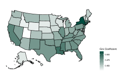
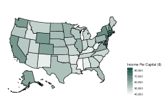
Figure 1: Descriptive statistics on the US map: (a) Gini Coefficient; (b) Household Income Per Capital; (c) Unemployment Rate.

Table 1: Mean and median values of GDP contribution for each industry across all 51 states in the United States

Industry List	Mean	Median
1) Agriculture, forestry, fishing and hunting	0.0129	0.0075
2) Mining, quarrying, and oil and gas extraction	0.0222	0.0032
3) Utilities	0.0177	0.0169
4) Construction	0.0435	0.0410
5) Manufacturing	0.1105	0.1045
6) Wholesale trade	0.0568	0.0559
7) Retail trade	0.0583	0.0567
8) Transportation and warehousing	0.0374	0.0332
9) Information	0.0371	0.0302
10) Finance	0.2041	0.2041
11) Professional and business services	0.1152	0.1144
12) Educational services, health care, and social assistance	0.0929	0.0918
13) Arts, entertainment, recreation, accommodation, and food services	0.0453	0.0392
14) Other services except government and government enterprise	0.0229	0.0223
15) Federal civilian	0.0304	0.0194
16) State and local spending	0.0921	0.0894

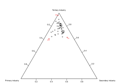
Figure 2: Ternary diagram of the U.S. 2019 intersectoral GDP contributions data for 51 states.

The intersectoral GDP contribution data are compositional data. Compositional data indicates the the relative amount of proportions of a whole and the data sums up to a constant value. The sample space of compositional data, called a simplex, is denoted by $\mathcal{S}^{k-1}=\{\bm{x}=[x_{1},...,x_{k}]\in\mathbb{R}^{k}|x_{i}\geq 0,i=1,...,k;\sum_{i=1}^{k}x_{i}=1\}$ where $k$ is the number of components. The intersectoral GDP shows the proportion of each industry’s contribution, and the contributions data of each state sum up to 1. If we do regression analysis directly with compositional data as a predictor, the compositional data will lead to the parameter identifiable issue in the linear regression. For example, if the real model is $y=1+2x_{1}+x_{2}$ where $y\in R$ and $\{x_{1},x_{2}\}\in\mathcal{S}^{1}$. We may obtain $y=2+x_{1}$ or $y=3-x_{2}$ as our estimated model which is consistent with the data, but the coefficients of $x_{1}$ and $x_{2}$ are not in agreement with our real model. In this paper, we will follow aitchison1982statistical and introduce log-contrast regression model, using Hessian matrix to avoid the parameter identifiable issue, which will be presented in the next section.

3 Methodology

3.1 Bayesian Log-Contrast Regression for Compositional Covariates

In this section, we will first describe a log-contrast regression model for compositional predictors. To identify potential links between intersectoral GDP contributions and Gini coefficients, a log-contrast regression with compositional predictors will be discussed. Suppose we observe $n$ independent observations of a continuous type response $y_{i}\in\mathbb{R}$, a $k$ dimensional compositional predictor $\tilde{\bm{X}}_{1i}=[x^{(1)}_{i1},\ldots,x^{(1)}_{ik}]^{\top}$, such that $\tilde{\bm{X}}_{1i}\in\mathcal{S}^{k-1}$, and another $p$ dimensional non-compositional predictor $\bm{X}_{2i}=[x^{(2)}_{i1},...,x^{(2)}_{ip}]^{\top}\in\mathbb{R}^{p}$. Denote $\bm{y}=[y_{1},\cdots,y_{n}]^{\top}$, $\tilde{\bm{X}}_{1}=[\tilde{\bm{X}}_{11},...,\tilde{\bm{X}}_{1n}]^{\top}$ and $\bm{X_{2}}=[\bm{X}_{21},...,\bm{X}_{2n}]^{\top}$. A linear model for $\bm{y}$ could be expressed as

$$\bm{y}=\tilde{\bm{X}}_{1}\overline{\bm{\beta}}+\bm{X}_{2}\bm{\eta}+\bm{\epsilon}$$

where $\overline{\bm{\beta}}$ is the $k$ dimensional regression coefficient, $\bm{\eta}$ is the $p$ dimensional regression coefficient, $\bm{\epsilon}\in\mathbb{R}^{n}$ is an $n$ dimensional random error vector with zero mean and variance $\sigma^{2}$. Ignoring the simplex structure of $\tilde{\bm{X}}_{1}$ would cause the issue of parameter identification in the linear regression of $\bm{y}$ on $\tilde{\bm{X}}_{1}$. One naive “remedy” is to exclude an arbitrary component of the compositional vector in the regression, but this may lead to a method that is not invariant to the choice of the removed component, since it affects both prediction and selection. Consequently, this would pose difficulty in properly interpreting and inferring the model. Following lin2014variable, we use a log-ratio transformation of the compositional data, such that the transformed data admit the familiar Euclidean geometry in $\mathcal{R}^{K-1}$. Specifically,

$$\bm{y}=\bm{Z}\tilde{\bm{\beta}}+\bm{X}_{2}\bm{\eta}+\bm{\epsilon},\qquad\text{s.t.}\quad\sum_{j=1}^{K}\tilde{\beta}_{j}=0,$$ (1)

where $\tilde{\bm{\beta}}=[\tilde{\beta}_{1},...,\tilde{\beta}_{k}]$ is the regression coefficient vector for the transformed design matrix $\bm{Z}$, which is the log-ratio transformation of $\tilde{\bm{X}}_{1}$. In order to remove the constraint of $\tilde{\bm{\beta}}$, a Helmert transformations is considered as

$$\bm{\beta}=\bm{H}\tilde{\bm{\beta}},$$ (2)

where $\bm{H}\in\mathbb{R}^{(K-1)\times K}$ is the Helmert sub-matrix (lancaster1965helmert) with the the first row omitted. The Helmert transformation matrix $\bm{H}$ is not a full row rank matrix. We propose an orthogonal projection (maynard2005drawing) by following the theorem, which provides a way to transform $\bm{\beta}$ to $\tilde{}\bm{\beta}$.

Theorem 1.

Let $\bm{H}=\bm{F}\bm{Q}$ be a full rank decomposition of $\bm{H}$. Then $\bm{F}\in\mathbb{R}^{(K-1)\times r}$ is a full column rank matrix and $\bm{Q}\in\mathbb{R}^{r\times K}$ is a full row rank matrix. Write $\bm{M}=(\bm{Q}^{\top},(\bm{Q}^{\bot})^{\top})^{\top}\in\mathbb{R}^{K\times K}$, where $\bm{Q}^{\bot}\in\mathbb{R}^{(K-r)\times K}$ is the orthogonal compliment of $\bm{Q}$ satisfying $\bm{Q}(\bm{Q}^{\bot})^{\top}=\mathbf{0}$. Let $\tilde{\bm{M}}=(\tilde{\bm{M}}_{1},\tilde{\bm{M}}_{2})=\bm{M}^{-1}$ with $\tilde{\bm{M}}_{1}\in\mathbb{R}^{K\times(K-1)}$. Then the inverse transformation of $\bm{\tilde{\beta}}$ is

$$\tilde{\bm{\beta}}=\tilde{\bm{M}}_{1}\bm{\beta}.$$ (3)

Based on the Theorem 1, we have the following linear regression model instead of a regression model with linear constraint

$$\bm{y}=\bm{X}_{1}\bm{\beta}+\bm{X}_{2}\bm{\eta}+\bm{\epsilon},$$ (4)

where $\bm{X}_{1}=\bm{Z}\tilde{\bm{M}}_{1}$. Thus, we eliminate the problem of dealing with compositional covariates by log-ratio transformation and omit the redundant dimension of $\bm{\beta}$ using the Hermert matrix. For (4), a joint prior for $\bm{\beta}$, $\bm{\eta}$ and $\sigma^{2}$ can be used to complete the Bayesian model.

3.2 Bayesian Spatially Clustered Regression

For many spatial economics data, regions may share the same predictor effects with their nearby regions. In the meanwhile, regions may share similar parameters regardless of their geographical distances, due to the similarities of regions’ demographical information such as population and tax rate. A spatially varying pattern for covariate effects may not be always valid. Based on the homogeneity pattern, we focus on the clustering of regression coefficients of compositional predictors. In our setting, we assume that the $n$ regression coefficient vectors can be clustered into $k$ groups. For known $k$ settings, a finite mixture model is a natural solution for probabilistic clustering. However, the performance of the estimation of cluster assignments highly relies on the pre-specified number of clusters, it may ignore the uncertainty in the number of clusters and cause redundant cluster assignments. The Bayesian nonparametric method is a natural solution for simultaneously estimating the number of clusters and cluster configurations. Suppose each individual $i$ carries a latent group $z_{i}$. The conditional distributions of $z_{1},\ldots,z_{n}$ could be formulated as Chinese restaurant process (CRP, pitman1995exchangeable).

However, the CRP has been shown to produce redundant tail clusters, causing inconsistency in estimation for the number of clusters even with a large sample size. In addition, the spatial information among the states is not taken into consideration for the CRP. Another modification of the Dirichlet process mixture model is proposed, known as the mixture of finite mixtures (MFM) model, to mitigate the inconsistency issue (miller2018mixture). The MFM model can be formulated as

$$k\sim p(\cdot),\quad(\pi_{1},\ldots,\pi_{k})|k\sim\text{Dirichlet}(\gamma,\ldots,\gamma),\quad z_{i}|k,\bm{\pi}\sim\text{Cat}(k,\bm{\pi}),\quad i=1,\ldots,n,$$

with $p(\cdot)$ being the Poisson distribution function truncated to be positive (i.e., $k-1\sim\text{Poisson}(\lambda)$), and $\text{Cat}(k,\bm{\pi})$ is k-dimensional categorical distribution.

The MFM model can also be formulated as a similar restaurant process:

$$P\left(z_{i}=c|\bm{z}_{-i}\right)\propto\begin{cases}|c|+\gamma,&\text{ at an existing label $c$}\\ V_{n}(K^{*}+1)/V_{n}(K^{*})\gamma,&\text{ if $c$ is a new label}\end{cases},$$ (5)

where $K^{*}$ is the number of existing clusters and the coefficient $V_{n}(w)$ is computed as

$$V_{n}(w)=\sum_{k=1}^{\infty}\frac{k(w)}{(\gamma k)^{(n)}}p(k),$$

where $k^{(m)}=k(k+1)\ldots(k+m-1)$ and $k(m)=k(k-1)\ldots(k-m+1)$, with $k^{(0)}=1$ and $k(0)=1$. The coefficient $V_{n}(w)$ also slows down the rate of introducing new clusters to existing ones, which can avoid having many tiny extraneous groups in the cluster. Another important consideration for spatial homogeneity learning is borrowing spatial information. Our remedy is combining Markov random field (MRF, orbanz2008nonparametric) with MFM. The dependence structure of different variables can be represented by a graph, with vertices representing random variables and an edge connecting two vertices indicating statistical dependence. The Markov random field constrained MFM (MRFC-MFM) consists of an interaction term modeled by an MRF cost function that captures spatial interactions among vertices and a vertex-wise term modeled by an MFM. Denote $\bm{\theta}(s_{i})$ by the parameter of the location $i$. The joint prior for $\{\theta(s_{i}):1\leq i\leq n\}$ for MRFC-MFM is given as

$$\pi(\bm{\theta}(s_{1}),\ldots,\bm{\theta}(s_{n}))\propto P(\bm{\theta}(s_{1}),\ldots,\bm{\theta}(s_{n}))M(\bm{\theta}(s_{1}),\ldots,\bm{\theta}(s_{n})|\mathcal{G}),$$ (6)

with $P(\bm{\theta}(s_{1}),\ldots,\bm{\theta}(s_{n}))$ as the part of the joint prior distribution for $\bm{\theta}(s_{1}),\ldots,\bm{\theta}(s_{n})$ induced by MFM, and $M(\bm{\theta}(s_{1}),\ldots,\bm{\theta}(s_{n})|\mathcal{G})$ as anther part of joint prior distribution which is induced by Markov random field given a graph structure $\mathcal{G}$. The pre-specified $\mathcal{G}$ is defined as an unweighed graph with vertices $V_{\mathcal{G}}=(v_{1},\ldots,v_{n})$ representing random variables at $n$ spatial locations, $E_{\mathcal{G}}$ denoting a set of edges representing statistical dependence among vertices. By the Hammersley-Clifford theorem (clifford1971markov), the corresponding conditional distributions of $M(\bm{\theta}(s_{1}),\ldots,\bm{\theta}(s_{n})|\mathcal{G})$ enjoy the Markov property, i.e., $M(\bm{\theta}(s_{i})|\bm{\theta}(s_{-i}))=M(\bm{\theta}(s_{i})|\bm{\theta}(s_{\partial(i)}))$, where $\bm{\theta}(s_{-i})=(\bm{\theta}(s_{1}),\ldots,\bm{\theta}(s_{i-1}),\bm{\theta}(s_{i+1}),\ldots,\bm{\theta}(s_{n}))$ and $\partial(i)$ denotes the set of neighborhood locations of $s_{i}$ given the graph $\mathcal{G}$.

Proposition 1.

Let $n_{k}^{(-i)}$ denote the size of the $k$-th cluster excluding $\bm{\theta}(s_{i})$, $K^{*}$ denote the number of clusters excluding the $i$-th observation, $\bm{\theta}^{*}_{1},\ldots,\bm{\theta}^{*}_{K^{*}}$ denote $K^{*}$ distinguished parameters and assume $M(\bm{\theta}(s_{1}),\ldots,\bm{\theta}(s_{n})|\mathcal{G})=\frac{1}{Z_{H}}\text{exp}\{-H(\bm{\theta}(s_{1}),\ldots,\bm{\theta}(s_{n})|\mathcal{G})\}$, where $\frac{1}{Z_{H}}$ is the normalizing constant. The conditional distribution of an MRFC-MFM takes the form

$$\Pi(\bm{\theta}(s_{i})\mid\bm{\theta}(s_{-i}))\propto\sum_{k=1}^{K^{*}}(n_{k}^{(-i)}+\gamma)\frac{1}{Z_{H}}\exp(-H(\bm{\theta}(s_{i})\mid\bm{\theta}(s_{-i})))\delta_{\bm{\theta}^{*}_{k}}(\bm{\theta}(s_{i}))+\dfrac{V_{n}(K^{*}+1)}{V_{n}(K^{*})}\dfrac{\gamma}{Z_{H}}G_{0}(\bm{\theta}(s_{i}))$$ (7)

where

$$H(\bm{\theta}(s_{i})\mid\bm{\theta}(s_{-i}))=-\lambda\sum_{\ell\in\partial(i)}I(z_{\ell}=z_{i}).$$ (8)

$\delta_{\bm{\theta}^{*}_{k}}(\bm{\theta}(s_{i}))$ is the distribution concentrated at a single point, $\bm{\theta}^{*}_{k}$, and a base measure $G_{0}$ is defined the same as the Dirichlet process (neal2000markov).

In Proposition 1, $\lambda$ is a spatial smoothness parameter. A larger value of $\lambda$ indicates stronger spatial smoothing. Proposition (1) gives a similar condition distribution with traditional Chinese resturant processs. Combining (7) and (8), we can have a similar conditional distribution for $z_{1},\ldots,z_{n}$ as

$$P\left(z_{i}|\bm{z}_{-i}\right)\propto\begin{cases}(|c|+\gamma)\text{exp}[\lambda\sum_{l\in\partial_{s}(i)}I(z_{l}=z_{i})],&\text{at an existing labeled c}\\ V_{n}(K^{*}+1)/V_{n}(K^{*})\gamma,&\text{if c is new cluster}\end{cases}.$$ (9)

The above urn scheme offers a similar Chinese restaurant process interpretation (neal2000markov) of the proposed prior: the probability of customer $i$ sitting at a table depends not only on the number of existing customers seated at that table but also on spatial relationships between the $i$-th customer with existing customers. Compared with traditional MFM and CRP, this Pólya urn scheme will let nearby states have a higher probability being clustered together when $\lambda\neq 0$. This will enforce the locally contiguous clusters. The globally discontiguous clusters will be learned from the data itself. Compared with existing Bayesian approaches (lu2007bayesian; li2015bayesian; gao2023spatial; aiello2023detecting) for spatial clustering detection, the clustering labels can be inferred directly by the posterior estimates without any FDR-based post selection procedures.

3.3 Bayesian Hierarchical Model

Consider the following specifications of the data models for linking state-specific Gini coefficients ($y_{i},i=1,\ldots,n$) and both transformed compositional predictors $\bm{X}_{1i}=\bm{Z}_{i}\tilde{\bm{M}}_{1}$ and non-compositional predictors $\bm{X}_{i2}$

$$y_{i}|\bm{X}_{1i},\bm{X}_{2i},\bm{\beta}(s_{i}),\bm{\eta}\sim\mathcal{N}(\bm{X}_{1i}\bm{\beta}(s_{i})+\bm{X}_{2i}\bm{\eta},\sigma^{2}(s_{i})),$$ (10)

where $\bm{\beta}(s_{i})$ is spatially varying coefficients for compositional predictors, $\bm{\eta}$ is spatially constant coefficients for non-compositional predictors, and $\sigma^{2}(s_{i})$ is spatially varying variance.

For spatially constant coefficients $\bm{\eta}$, a multivariate normal prior is given as

$$\bm{\eta}\sim\mathcal{N}_{p}(\bm{\eta}_{0},\bm{V}_{0}),$$ (11)

where hyperparameters $\bm{\eta}_{0}=\bm{0}_{p}$ and $\bm{V}_{0}=100\bm{I}_{p}$. In order to capture the spatially clustered pattern of regression coefficients for compositional predictors, a MRFC-MFM prior is proposed for $\bm{\theta}(s_{i})=(\bm{\beta}^{\top}(s_{i}),\sigma^{2}(s_{i}))^{\top}$ with Normal-Inverse-Gamma (NIG) base distribution as

$$\begin{split}\bm{\theta}(s_{1}),\ldots,\bm{\theta}(s_{n})&\sim M(\bm{\theta}(s_{1}),\ldots,\bm{\theta}(s_{n})|\mathcal{G})\prod_{i=1}^{n}G(\bm{\theta}(s_{i})),\\ G(\bm{\theta}(s_{i}))|\pi_{1},\ldots,\pi_{K},K&\sim\sum_{\ell=1}^{K}\pi_{\ell}\text{NIG}(\bm{\tau}_{0},\Sigma_{0},a_{0},b_{0}),\\ \pi_{1},\ldots,\pi_{K}|K&\sim\text{Dirichlet}(\gamma,\ldots,\gamma),\\ K-1&\sim\text{Poisson}(\zeta),\end{split}$$ (12)

where $\bm{\tau}_{0}=\bm{0},\bm{\Sigma}_{0}=\bm{I},a=0.01,b=0.01$, $\bm{\eta}_{0}=\bm{0}$ and $\bm{V}_{0}=100\bm{I_{p}}$ are the hyperparameters for NIG distribution, and $\zeta$ is pre-specified parameters for Poisson distribution. $M(\bm{\theta}(s_{1}),\ldots,\bm{\theta}(s_{n}))$ is part of joint prior induced by Markov random field given a graph structure $\mathcal{G}$. The $\mathcal{G}$ is the spatial adjacency structure in our simulation and application. In the rest of paper, we choose $\zeta=1$ and $\gamma=1$ as (miller2018mixture). Combining (10), (11), and (12), we finish our hierarchical model.

4 Bayesian Inference

In this section, we will introduce the MCMC sampling algorithm, post-MCMC inference method, and Bayesian model selection criterion.

4.1 MCMC Algorithm

Our goal is to sample from the posterior distribution of the unknown parameters $K$, $\bm{z}=(z_{1},...,z_{K}),\bm{\beta}=({\bm{\beta}_{1},...,\bm{\beta}_{K}}),\bm{\sigma^{2}}=({{\sigma_{1}^{2}},...,{\sigma_{K}^{2}}}),\bm{\eta}=(\eta_{1},...,\eta_{p})$. The marginalization over $K$ can avoid complicated reversible jump MCMC algorithms or even allocation samplers. For posterior computation we use a Gibbs sampler defined by the following propositions.

Proposition 2.

The full conditional distributions of $z_{i}$’s are given

$$P(z_{i}|\bm{z}_{-i},\bm{\beta},\bm{\sigma}^{2},\bm{\eta})\propto\left\{\begin{array}[]{l}\alpha_{1}f(y_{i};\bm{X}_{1i},\bm{X}_{2i},\bm{\beta}_{k},\bm{\eta}),\qquad\text{ at existing }k\\ \alpha_{2}g(y_{i};\tau_{0},\tau,\Sigma_{0},\Sigma,a_{0},b_{0},\bm{X}_{2i},\bm{\eta}),\qquad\text{if }k\text{ is a new cluster }\end{array}\right.$$

where