Mechanics and thermodynamics of contractile biopolymer networks

Abstract

Contractile biopolymer networks, such as the actomyosin meshwork of animal cells, are ubiquitous in living organisms. The active gel theory, which provides the thermodynamic framework for these materials, has been mostly used in conjunction with the assumption that the microstructure of the biopolymer network is based on rigid rods. However, experimentally, the actin network exhibits entropic elasticity. Here we combine an entropic elasticity kinetic theory, in the spirit of the Green and Tobolsky model of transiently crosslinked networks, with an active flux modelling biological activity. We determine this active flux using Onsager reciprocal relations and interpret the corresponding microscopic dynamics. We obtain a closed model of the macroscopic mechanical behaviour. We show how this model can be written using the framework of multiplicative strain gradient decomposition, which is convenient for the resolution of such problems.

1 Introduction

Active matter comprises a wide range of structures of mechanical relevance and features numerous means to perform mechanical work with and within them Taber, (1995). Among those however, within the animal kingdom, biopolymer networks endowed with the ability to self-contract are arguably the most pervasive, both inside the cells and outside of them. Muscle contraction constitutes a classical example of this. It can be idealised as the relative sliding of parallelly-organised filaments of actin and myosin, actuated by the conformation change of the myosin, which itself is powered by the energy released by ATP hydrolysis Huxley, (1957); Caruel and Truskinovsky, (2018). Actin and myosin are also essential players of the cytoskeleton involved in an extensive range of active mechanical behaviours of cells Bray and White, (1988); Mitchison and Cramer, (1996); Recho et al., (2013), where they form a thin crosslinked network apposed to the impermeable plasma membrane Salbreux et al., (2012), called actomyosin. Outside of cells, extracellular matrices (ECM) are based on networks of biological polymers that form soft elastic gels Levental et al., (2007) and within which cells exert forces in a variety of ways Delvoye et al., (1991); Bertinetti et al., (2015); Han et al., (2018). The very rich behaviour of contractile networks has also been explored in vitro using purified gels of biological proteins Nedelec et al., (1997); Koenderink et al., (2009); Stuhrmann et al., (2012). While ECM networks and in vitro gels have properties that are distinct from those of cytoskeletal actomyosin, the geometry of the microstructure and the origins of active stress bear interesting similarities.

Continuum modelling approaches have been able to reproduce a number of the behaviours of the actomyosin cytoskeleton by the introduction of an active stress as a driving force within a liquid-like material modelling the network Dembo and Harlow, (1986). This active stress can be interpreted as a dynamic prestress Erlich et al., (2022), allowing to draw analogies with the residual stress which is observed in solid-like tissue Fung, (1991); Goriely and Vandiver, (2010). The theory of active gels Kruse et al., (2005); Jülicher et al., (2007), drawing from the hydrodynamics of suspensions of orientable objects endowed with active stresses Marchetti et al., (2013), has provided a sound thermodynamic framework for the generation of this active stress by molecular motors. A link has been done with materials whose microstructure relies on rigid filaments Liverpool and Marchetti, (2006); Hawkins and Liverpool, (2014). Actin filaments are semiflexible, however the elasticity of the resulting networks has been shown to be of entropic nature Gardel et al., (2004). It is thus interesting to consider in what measure the entropic elasticity of the microstructure modifies the constitutive relations of active biopolymer networks.

Here, we consider a microstructure of freely-jointed chains, exhibiting entropic elasticity, which form a percolating network through high-affinity but reversible binding. In addition to affine deformations, we allow for motion due to the action of active crosslinks, which model molecular motors. The thermodynamics of this system is then written within the constraints of this particular microstructure, which allows us to propose microscopic interpretations of the Onsager relations.

Section 2 presents the kinetic model, its thermodynamics and is concluded with a closed mechanical model. Section 3 presents a multiplicative decomposition approach that allows to recover this model and is convenient for its resolution and for numerical approaches. Section 4 concludes the paper with a simple example.

2 A kinetic theory of contractile biopolymer networks

2.1 Kinetics of active temporary networks

In this section, we follow the approach of transiently crosslinked networks Green and Tobolsky, (1946); Yamamoto, (1956) and combine it explicitly with an elastic dumbbell model Bird et al., (1987); Larson, (1988, 1999) to describe the dynamics of unbound chains. This will make possible the interpretation of the dissipation in the next section. The other novelty here is the presence of an additional flux, which represent the active dynamics of the network. It is not specified in this section how this flux depends on other fields, this will be done in view of the thermodynamics of the system in Section 2.5, allowing us to reconcile phenomenological kinetic approaches Étienne et al., (2015) with generic thermodynamic considerations Kruse et al., (2005).

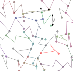
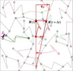
A B C

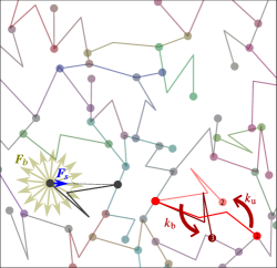
Figure 1: Network model. A, Chains made of a finite number of Kuhn steps (three in this schematic) of length $\beta^{-1}$ each are described by the end-to-end vector $\underaccent{\sim}{\boldsymbol{{R}}}$. They can connect to other chains at their ends. B, If a global deformation $\underaccent{\sim}{\boldsymbol{{\nabla}}}\underaccent{\sim}{\boldsymbol{{v}}}$ exists, bound chains are affinely deformed, Eq. (1). The additional active flux $\underaccent{\sim}{\boldsymbol{{j}}}_{\mathrm{\!a}}$ is described in Section 2.5. C, Unbound end of a chain is submitted to spring force $\underaccent{\sim}{\boldsymbol{{F}}}_{s}$ and to a Brownian force that averages to $\underaccent{\sim}{\boldsymbol{{F}}}_{b}$ over short times. They relax fast to a configuration where those forces balance. Bound ends (configuration 1) unbind at rate $k_{\mathrm{u}}$ and relax (configuration 2). They can then rebind at rate $k_{\mathrm{b}}$ (configuration 3) but do so in their relaxed state.

We consider the biopolymer network as an assembly of polymer molecules of idealised elastic freely-jointed chains in a viscous liquid (e.g. the cytosol). The chains can be represented by elastic dumbbells Larson, (1999), that is, a nonbendable spring joining two beads which can bind to beads of neighbouring molecules. For each chain, the end-to-end vector $\underaccent{\sim}{\boldsymbol{{R}}}(t)\in\mathbb{R}^{3}$, called strand, connects each of the dumbbell beads, see Fig. 1.

We assume a high affinity between the chains and that consequently, a large connected component of chains forms a macroscopic network. Within this percolated component, each "bound" strand $\underaccent{\sim}{\boldsymbol{{R}}}_{\mathrm{b}}$ is assumed to deform affinely with the network. Thus, if the macroscopic velocity gradient $\underaccent{\approx}{\boldsymbol{{{\ell}}}}\,^{\!\mathsf{T}}$ varies over distances much greater than the typical length of $\underaccent{\sim}{\boldsymbol{{R}}}_{\mathrm{b}}$, the dynamic of $\underaccent{\sim}{\boldsymbol{{R}}}_{\mathrm{b}}$ is given by :

$$\dot{\underaccent{\sim}{\boldsymbol{{R}}}}_{\mathrm{b}}=\underaccent{\approx}{\boldsymbol{{{\ell}}}}\cdot\underaccent{\sim}{\boldsymbol{{R}}}_{\mathrm{b}}+\underaccent{\sim}{\boldsymbol{{j}}}_{\mathrm{\!a}}.$$ (1)

Here $\underaccent{\sim}{\boldsymbol{{j}}}_{\mathrm{\!a}}$ represents some active process that remodels the network, yet unspecified, the case of passive transiently crosslinked networks being $\underaccent{\sim}{\boldsymbol{{j}}}_{\mathrm{\!a}}=\underaccent{\sim}{\boldsymbol{{0}}}$.

However, transiently, one of the beads in a dumbbell can disconnect from this network, undergo different dynamics for a brief duration, and then reconnect to it. For simplicity, we do not consider the quadratically rare cases where both beads disconnect. The Langevin equation ruling the $\underaccent{\sim}{\boldsymbol{{R}}}_{\mathrm{u}}$ dynamics is then:

$$\zeta(\dot{\underaccent{\sim}{\boldsymbol{{R}}}}_{\mathrm{u}}-\underaccent{\approx}{\boldsymbol{{{\ell}}}}\cdot\underaccent{\sim}{\boldsymbol{{R}}}_{\mathrm{u}})=\underaccent{\sim}{\boldsymbol{{F}}}_{s}+\underaccent{\sim}{\boldsymbol{{F}}}_{b},$$ (2)

where $\underaccent{\sim}{\boldsymbol{{F}}}_{s}$ and $\underaccent{\sim}{\boldsymbol{{F}}}_{b}$ are respectively the internal spring force of the chain and the Brownian force due to the thermal fluctuations in the liquid. The liquid is considered to have the same velocity locally as the network, thus the viscous drag force on the free end of the chain is proportional to the difference between its relative velocity and $\underaccent{\approx}{\boldsymbol{{{\ell}}}}\cdot\underaccent{\sim}{\boldsymbol{{R}}}_{\mathrm{u}}$, where we have again considered that the variations of $\underaccent{\approx}{\boldsymbol{{{\ell}}}}$ are on a larger spatial scale than the typical $\underaccent{\sim}{\boldsymbol{{R}}}_{\mathrm{u}}$.

Up to a factor two on the drag coefficient $\zeta$ (due to the bound state of one of the beads), this is the same Langevin equation as the one used to derive dumbbell models Bird et al., (1987); Larson, (1988, 1999), and the expressions of the forces are the same:

$$\underaccent{\sim}{\boldsymbol{{F}}}_{b} =\sqrt{2k_{B}T}\underaccent{\sim}{\boldsymbol{{\eta}}}(t)$$ (3)

$$\underaccent{\sim}{\boldsymbol{{F}}}_{s} =-\kappa\underaccent{\sim}{\boldsymbol{{R}}}_{u}.$$ (4)

The form of $\underaccent{\sim}{\boldsymbol{{F}}}_{b}$, with $k_{B}$ the Boltzmann constant, $T$ the temperature and $\underaccent{\sim}{\boldsymbol{{\eta}}}$ an isotropic white noise is chosen to guarantee the equipartition of energy in the permanent regime Larson, (1988) for the (passive) unbound phase. The strand stiffness $\kappa=2k_{B}T\beta^{2}$ is normalized with the thermal energy where $\beta^{-1}$ is called the Kuhn length of the freely jointed segments that form the Gaussian chains.

Introducing the probabilities to observe bounded and unbounded strands of a certain length $\psi_{\mathrm{b,u}}(\underaccent{\sim}{\boldsymbol{{r}}},t)=\operatorname{{Prob}}(\underaccent{\sim}{\boldsymbol{{R}}}_{\mathrm{b,u}}(t)=\underaccent{\sim}{\boldsymbol{{r}}})$, the Fokker-Planck dynamic associated to the Langevin process (1)-(2) take the form:

$$\frac{\partial\psi_{\mathrm{b}}}{\partial t}+\underaccent{\sim}{\boldsymbol{{\nabla}}}_{\!{\boldsymbol{{r}}}}\cdot\left(\psi_{\mathrm{b}}(\underaccent{\approx}{\boldsymbol{{{\ell}}}}\cdot\underaccent{\sim}{\boldsymbol{{r}}}+\underaccent{\sim}{\boldsymbol{{j}}}_{\mathrm{\!a}})\right) =-k_{\mathrm{u}}\mathcal{K}_{u}(\psi_{\mathrm{u}},\psi_{\mathrm{b}})$$ (5a)

$$\frac{\partial\psi_{\mathrm{u}}}{\partial t}+\underaccent{\sim}{\boldsymbol{{\nabla}}}_{\!{\boldsymbol{{r}}}}\cdot\left(\psi_{\mathrm{u}}(\underaccent{\approx}{\boldsymbol{{{\ell}}}}\cdot\underaccent{\sim}{\boldsymbol{{r}}}/\zeta-\kappa\underaccent{\sim}{\boldsymbol{{r}}})-k_{B}T\underaccent{\sim}{\boldsymbol{{\nabla}}}_{\!{\boldsymbol{{r}}}}\psi_{\mathrm{u}}\right) =k_{\mathrm{u}}\mathcal{K}_{u}(\psi_{\mathrm{u}},\psi_{\mathrm{b}})$$ (5b)

where we define the characteristic unbinding rate $k_{\mathrm{u}}$, and the reaction term $\mathcal{K}_{u}$. In the sequel we will take the simplest possible reaction term, $\mathcal{K}_{u}=\psi_{\mathrm{u}}-(k_{\mathrm{b}}/k_{\mathrm{u}})\psi_{\mathrm{b}}$, with $k_{\mathrm{b}}$ a constant binding rate. Note that the total probability distribution of the two populations with $\psi=\psi_{\mathrm{u}}+\psi_{\mathrm{b}}$ sums to one.

We now consider the limit of low drag resistance to the motion of unbound chains: this corresponds to a fast relaxation to equilibrium whenever one of the ends of a chain unbinds from the network, and thus $\zeta k_{\mathrm{u}}/\kappa\ll 1$. Thus we can expand $\psi_{\mathrm{u}}$ as $\psi_{\mathrm{u}}=a_{\mathrm{u}}\psi_{0}+O(a_{\mathrm{u}}\zeta k_{\mathrm{u}}/\kappa)$ where $\psi_{0}$ solves Eq. (5b) to the first order and corresponds to the Gaussian distribution that freely-jointed chains adopt at rest for $\underaccent{\sim}{\boldsymbol{{F}}}_{s}+\underaccent{\sim}{\boldsymbol{{F}}}_{b}=0$, leading to $-\psi_{0}\kappa\underaccent{\sim}{\boldsymbol{{r}}}-k_{B}T\underaccent{\sim}{\boldsymbol{{\nabla}}}_{\!{\boldsymbol{{r}}}}\psi_{0}=0$ and thus $\psi_{0}=(\kappa/(2\pi k_{B}T))^{3/2}\exp(-\kappa{\boldsymbol{{r}}}^{2}/(2k_{B}T))$. The fraction of bound chains $a_{\mathrm{u}}$ in the permanent regime is a constant set by the integral constraint $\int_{\mathbb{R}^{3}~{}\!\!\!}\mathcal{K}_{u}(\psi_{\mathrm{b}},\psi_{\mathrm{u}})\>\text{d}{\boldsymbol{{r}}}=0$. See Appendix A for the first order expansion.

The time dependent part of $\psi$ is thus reduced to $\psi_{\mathrm{b}}$, and from Eq. (5a) we have:

$$\frac{\partial\psi_{\mathrm{b}}}{\partial t}+\underaccent{\sim}{\boldsymbol{{\nabla}}}_{\!{\boldsymbol{{r}}}}\cdot\left(\psi_{\mathrm{b}}(\underaccent{\approx}{\boldsymbol{{{\ell}}}}\cdot\underaccent{\sim}{\boldsymbol{{r}}}+\underaccent{\sim}{\boldsymbol{{j}}}_{\mathrm{\!a}})\right) =-k_{\mathrm{u}}\mathcal{K}_{0}(\psi_{\mathrm{b}})+O\left(\frac{\zeta k_{\mathrm{u}}^{2}}{\kappa}\right)$$ (6)

For $\underaccent{\sim}{\boldsymbol{{j}}}_{\mathrm{\!a}}=\underaccent{\sim}{\boldsymbol{{0}}}$ and since the first order approximation is $k_{\mathrm{u}}\mathcal{K}_{0}(\psi_{\mathrm{b}})=k_{\mathrm{u}}\psi_{\mathrm{b}}-k_{\mathrm{b}}a_{\mathrm{u}}\psi_{0}$, Eq. (6) is the same Smoluchowski equation of Yamamoto, (1956) for $\psi_{\mathrm{b}}$, this is known to lead to the upper-convected Maxwell constitutive equation for stress–strain relation (Larson,, 1988, p. 168), with a relaxation time equal to $k_{\mathrm{u}}^{-1}$. Note that the upper-convected Maxwell stress–strain relation, with relaxation time equal to $\zeta/\kappa$, is also the result for unbound chains only, i.e. Eqs. (5b),(2) with $\mathcal{K}_{u}=0$ but finite $\zeta$.

The classical derivation uses the procedure of integrating the forces exerted by this distribution of springs on an elementary volume, but the same result can be obtained using the virtual work principle (Larson,, 1988, p. 33). As seen below, this is useful in the context of active systems.

2.2 The stress tensor

For our isothermal system, the total dissipation can be written as:

$$\mathcal{D}=\frac{\delta W}{\delta t}-\frac{\mathrm{d}\mathcal{F}}{\mathrm{d}t}$$

where the terms are respectively the rate of work and the Gibbs free energy variations.

Let $\Omega(t)$ be the domain occupied by the material at time $t$. The trajectory of material points of the network is denoted $\underaccent{\sim}{\boldsymbol{{x}}}=\underaccent{\sim}{\boldsymbol{{\chi}}}(\underaccent{\sim}{\boldsymbol{{X}}},t)\in\Omega(t)$ where $\underaccent{\sim}{\boldsymbol{{X}}}\in\Omega(0)$ is the initial position at time $t=0$. We define the deformation as $\underaccent{\hskip 0.70004pt\approx}{\boldsymbol{\mathbf{F}}}(\underaccent{\sim}{\boldsymbol{{X}}},t)=\nabla_{{\boldsymbol{{X}}}}\underaccent{\sim}{\boldsymbol{{\chi}}}(\underaccent{\sim}{\boldsymbol{{X}}},t)$. The velocity is

$$\underaccent{\sim}{\boldsymbol{{v}}}=\frac{\partial\underaccent{\sim}{\boldsymbol{{\chi}}}}{\partial t}(\underaccent{\sim}{\boldsymbol{{\chi}}}^{-1}(\underaccent{\sim}{\boldsymbol{{x}}},t),t),$$

and we identify $\underaccent{\approx}{\boldsymbol{{{\ell}}}}=\underaccent{\sim}{\boldsymbol{{\nabla}}}_{\!{\boldsymbol{{x}}}}\underaccent{\sim}{\boldsymbol{{v}}}^{\!\mathsf{T}}$. To remain in the conditions above, it is assumed that $\underaccent{\hskip 0.70004pt\approx}{\boldsymbol{\mathbf{F}}}(\underaccent{\sim}{\boldsymbol{{X}}},t)$ varies in space over distances much longer than the typical length of a strand $\underaccent{\sim}{\boldsymbol{{R}}}$. We assume that inertia and body forces acting on the system are negligible, leading to the momentum balance equations:

$$-\underaccent{\sim}{\boldsymbol{{\nabla}}}p+\underaccent{\sim}{\boldsymbol{{\nabla}}}\cdot\underaccent{\hskip 0.70004pt\approx}{\boldsymbol{\mathbf{\sigma}}} =\underaccent{\sim}{\boldsymbol{{0}}} \text{in }\Omega(t)$$ (7a)

$$-p\underaccent{\sim}{\boldsymbol{{n}}}+\underaccent{\hskip 0.70004pt\approx}{\boldsymbol{\mathbf{\sigma}}}\cdot\underaccent{\sim}{\boldsymbol{{n}}} =\underaccent{\sim}{\boldsymbol{{f}}}_{\text{ext}} \text{on }\partial\Omega(t)$$ (7b)

where $p$ is the fluid pressure, $\underaccent{\hskip 0.70004pt\approx}{\boldsymbol{\mathbf{\sigma}}}$ the stress tensor and $\underaccent{\sim}{\boldsymbol{{f}}}_{\text{ext}}$ external forces applied on the system’s boundaries. Thus, the rate of work is equal to the work performed on the system’s boundary, and from Eq. (7) and using the symmetry of $\underaccent{\hskip 0.70004pt\approx}{\boldsymbol{\mathbf{\sigma}}}$,

$$\frac{\delta W}{\delta t}=\int_{\partial\Omega(t)\!\!\!}\underaccent{\sim}{\boldsymbol{{f}}}_{\text{ext}}\cdot\underaccent{\sim}{\boldsymbol{{n}}}\>\text{d}{\boldsymbol{{{\boldsymbol{{s}}}}}}=\int_{\Omega(t)\!\!\!}(\underaccent{\hskip 0.70004pt\approx}{\boldsymbol{\mathbf{\sigma}}}-p\underaccent{\hskip 0.70004pt\approx}{\boldsymbol{\mathbf{I}}}):\underaccent{\approx}{\boldsymbol{{{d}}}}\,\>\text{d}{\boldsymbol{{x}}}$$ (8)

with $\underaccent{\approx}{\boldsymbol{{{d}}}}=\frac{1}{2}(\underaccent{\approx}{\boldsymbol{{{\ell}}}}+\underaccent{\approx}{\boldsymbol{{{\ell}}}}^{\!\mathsf{T}})$.

Let us denote $\nu(\underaccent{\sim}{\boldsymbol{{x}}})$ the number of chains per unit volume within $\Omega(t)$. Mass conservation gives

$$\frac{\partial\nu}{\partial t}+\underaccent{\sim}{\boldsymbol{{\nabla}}}\cdot(\nu\underaccent{\sim}{\boldsymbol{{v}}}) =0 \text{in }\Omega(t)$$ (9a)

$$\nu(\underaccent{\sim}{\boldsymbol{{v}}}-\underaccent{\sim}{\boldsymbol{{v}}}_{b})\cdot\underaccent{\sim}{\boldsymbol{{n}}} =0 \text{on }\partial\Omega(t)$$ (9b)

$$\nu(t=0) =\nu_{0} \text{in }\Omega_{0}=\Omega(0)$$ (9c)

where $\underaccent{\sim}{\boldsymbol{{v}}}_{b}(t)$ is the velocity of $\partial\Omega(t)$, which from the above has a normal component equal to $\underaccent{\sim}{\boldsymbol{{v}}}$. Following Larson, (1988, p. 33), the elastic contribution of $\nu$ chains per unit volume to the Gibbs free energy is

$$\nu\varphi_{\mathrm{e}}:= \frac{1}{2}\nu\kappa\int_{\mathbb{R}^{3}\!\!\!}\psi(\underaccent{\sim}{\boldsymbol{{r}}})\underaccent{\sim}{\boldsymbol{{r}}}^{2}\>\text{d}{\boldsymbol{{r}}}.$$

We write the Gibbs free energy as:

$${\mathcal{F}}=\int_{\Omega_{t}\!\!\!}\nu\varphi\>\text{d}{\boldsymbol{{x}}}$$

where $\varphi=\varphi_{\mathrm{e}}+\varphi_{\mathrm{a}}$, and $\varphi_{\mathrm{a}}$ are anelastic contributions. The free energy variations are:

$$\frac{\mathrm{d}\mathcal{F}}{\mathrm{d}t} =\int_{\Omega_{t}\!\!\!}\left(\frac{\partial\nu}{\partial t}\varphi+\nu\frac{\partial\varphi}{\partial t}\right)\>\text{d}{\boldsymbol{{x}}}=\int_{\Omega_{t}\!\!\!}\nu\frac{\mathrm{d}\varphi}{\mathrm{d}t}\>\text{d}{\boldsymbol{{x}}}$$ (10)

where we have used Eq. (9) and one integration by parts.

Since in the limit $\zeta\rightarrow 0$, $\psi_{\mathrm{u}}$ is time-independent, the elastic contributions to free energy density variations can be deduced from the Smoluchowski Eq. (6):

$$\nu\frac{\mathrm{d}\varphi_{\mathrm{e}}}{\mathrm{d}t} =\frac{1}{2}\nu\kappa\int_{\mathbb{R}^{3}\!\!\!}\frac{\partial\psi_{\mathrm{b}}}{\partial t}(\underaccent{\sim}{\boldsymbol{{r}}})\underaccent{\sim}{\boldsymbol{{r}}}^{2}\>\text{d}{\boldsymbol{{r}}}$$

$$\stackrel{{\scriptstyle\text{IbP}}}{{=}}\frac{1}{2}\nu\kappa\int_{\mathbb{R}^{3}\!\!\!}\psi_{\mathrm{b}}(\underaccent{\sim}{\boldsymbol{{r}}}\cdot\underaccent{\sim}{\boldsymbol{{\nabla}}}_{\!{\boldsymbol{{x}}}}\underaccent{\sim}{\boldsymbol{{v}}}+\underaccent{\sim}{\boldsymbol{{j}}}_{\mathrm{\!a}})\cdot\underaccent{\sim}{\boldsymbol{{\nabla}}}_{\!{\boldsymbol{{r}}}}\underaccent{\sim}{\boldsymbol{{r}}}^{2}\>\text{d}{\boldsymbol{{r}}}-\frac{1}{2}\nu\kappa k_{\mathrm{u}}\int_{\mathbb{R}^{3}\!\!\!}\mathcal{K}_{0}(\psi_{\mathrm{b}})\underaccent{\sim}{\boldsymbol{{r}}}^{2}\>\text{d}{\boldsymbol{{r}}}$$

$$=\nu\kappa\left(\langle\underaccent{\sim}{\boldsymbol{{r}}}\underaccent{\sim}{\boldsymbol{{r}}}\rangle_{\mathrm{b}}:\underaccent{\approx}{\boldsymbol{{{d}}}}+\langle\underaccent{\sim}{\boldsymbol{{j}}}_{\mathrm{\!a}}\cdot\underaccent{\sim}{\boldsymbol{{r}}}\rangle_{\mathrm{b}}-\frac{1}{2}k_{\mathrm{u}}\int_{\mathbb{R}^{3}\!\!\!}\mathcal{K}_{0}(\psi_{\mathrm{b}})\underaccent{\sim}{\boldsymbol{{r}}}^{2}\>\text{d}{\boldsymbol{{r}}}\right)$$

where $\langle\,\cdot\,\rangle_{\mathrm{b}}=\int_{\mathbb{R}^{3}~{}\!\!\!}\psi_{\mathrm{b}}\,\cdot\,\>\text{d}{\boldsymbol{{r}}}$. This brings us to define the microstructure (or texture) tensor $\underaccent{\hskip 0.70004pt\approx}{\boldsymbol{\mathbf{A}}}=\langle\underaccent{\sim}{\boldsymbol{{r}}}\underaccent{\sim}{\boldsymbol{{r}}}\rangle_{\mathrm{b}}$.

We are now in a position to identify the different terms in the dissipation,

$$\mathcal{D} =\mathcal{D}_{0}+\mathcal{R}-\frac{\mathrm{d}\mathcal{F}_{\!\mathrm{a}}}{\mathrm{d}t}$$

where the first term is a dissipation induced by the deformation rate:

$$\mathcal{D}_{0} =\int_{\Omega(t)\!\!\!}\left(\underaccent{\hskip 0.70004pt\approx}{\boldsymbol{\mathbf{\sigma}}}-p\underaccent{\hskip 0.70004pt\approx}{\boldsymbol{\mathbf{I}}}-\nu\kappa\underaccent{\hskip 0.70004pt\approx}{\boldsymbol{\mathbf{A}}}\right):\underaccent{\approx}{\boldsymbol{{{d}}}}\>\text{d}{\boldsymbol{{x}}},$$

the second term is a dissipation associated with the relaxation of chains via the unbinding–rebinding dynamics:

$$\mathcal{R} =\nu\kappa k_{\mathrm{u}}\int_{\Omega(t)\,\!\!\!}\int_{\mathbb{R}^{3}\!\!\!}\mathcal{K}_{0}(\psi_{\mathrm{b}})\underaccent{\sim}{\boldsymbol{{r}}}^{2}\>\text{d}{\boldsymbol{{r}}}\>\text{d}{\boldsymbol{{x}}}$$

and the third is the power balance of active processes:

$$\frac{\mathrm{d}\mathcal{F}_{\!\mathrm{a}}}{\mathrm{d}t} =\int_{\Omega_{t}\!\!\!}\left(\nu\kappa\langle\underaccent{\sim}{\boldsymbol{{j}}}_{\mathrm{\!a}}\cdot\underaccent{\sim}{\boldsymbol{{r}}}\rangle_{\mathrm{b}}+\nu\frac{\mathrm{d}\varphi_{\mathrm{a}}}{\mathrm{d}t}\right)\>\text{d}{\boldsymbol{{x}}},$$

One can further decompose the stress term into deviatoric and isotropic components,

$$\mathcal{D}_{0}=\int_{\Omega(t)\!\!\!\!}\left(\!\operatorname{\mathbf{dev}}(\underaccent{\hskip 0.70004pt\approx}{\boldsymbol{\mathbf{\sigma}}}-\nu\kappa\underaccent{\hskip 0.70004pt\approx}{\boldsymbol{\mathbf{A}}}):\underaccent{\approx}{\boldsymbol{{{d}}}}+\left(\frac{1}{3}\operatorname{tr}(\underaccent{\hskip 0.70004pt\approx}{\boldsymbol{\mathbf{\sigma}}}-\nu\kappa\operatorname{tr}\underaccent{\hskip 0.70004pt\approx}{\boldsymbol{\mathbf{A}}})-p\right)\underaccent{\hskip 0.70004pt\approx}{\boldsymbol{\mathbf{I}}}:\underaccent{\approx}{\boldsymbol{{{d}}}}\right)\>\text{d}{\boldsymbol{{x}}}$$

The stress tensor can then be chosen as $\underaccent{\hskip 0.70004pt\approx}{\boldsymbol{\mathbf{\sigma}}}=\nu\kappa(\underaccent{\hskip 0.70004pt\approx}{\boldsymbol{\mathbf{A}}}-\underaccent{\hskip 0.70004pt\approx}{\boldsymbol{\mathbf{A}}}_{0})+2\mu\underaccent{\approx}{\boldsymbol{{{d}}}}+\mu_{b}(\underaccent{\sim}{\boldsymbol{{\nabla}}}\cdot\underaccent{\sim}{\boldsymbol{{v}}})\underaccent{\hskip 0.70004pt\approx}{\boldsymbol{\mathbf{I}}}$, where $\mu_{b}$ and $\mu$ are Lamé parameters corresponding to the dissipative contribution of the liquid bath. We have introduced an arbitrary isotropic tensor $\underaccent{\hskip 0.70004pt\approx}{\boldsymbol{\mathbf{A}}}_{0}=a_{0}\beta^{-2}\underaccent{\hskip 0.70004pt\approx}{\boldsymbol{\mathbf{I}}}$, where the value of $a_{0}$, corresponding to relaxed chains, will be derived in the next section. Its contribution to the stress can be balanced by the pressure term, indeed, the pressure $p$ can be chosen as a Lagrange multiplier which will enforce $\underaccent{\hskip 0.70004pt\approx}{\boldsymbol{\mathbf{I}}}:\underaccent{\approx}{\boldsymbol{{{d}}}}=\underaccent{\sim}{\boldsymbol{{\nabla}}}\cdot\underaccent{\sim}{\boldsymbol{{v}}}=0$ or any prescribed volume change. For both of these constitutive choices, we obtain

$$\mathcal{D}_{0}=\int_{\Omega(t)\!\!\!\!}\left(2\mu\underaccent{\hskip 0.70004pt\approx}{\boldsymbol{\mathbf{d}}}^{2}+\mu_{b}(\underaccent{\sim}{\boldsymbol{{\nabla}}}\cdot\underaccent{\sim}{\boldsymbol{{v}}})^{2}\right)\>\text{d}{\boldsymbol{{x}}},$$

thus only the liquid bath may contribute to a dissipation induced by the rate of deformation.

2.3 Constitutive equation of active networks

Having defined the stress tensor, we can proceed with the usual procedure of bead–spring models in order to determine the constitutive equation that relates stress and strain, and which consists in multiplying the Smoluchowski Eq. (6) by the tensor $\underaccent{\sim}{\boldsymbol{{r}}}\underaccent{\sim}{\boldsymbol{{r}}}$ and integrating over the phase space, which yields:

$$\frac{\mathrm{d}\underaccent{\hskip 0.70004pt\approx}{\boldsymbol{\mathbf{A}}}}{\mathrm{d}t}-\underaccent{\approx}{\boldsymbol{{{\ell}}}}\cdot\underaccent{\hskip 0.70004pt\approx}{\boldsymbol{\mathbf{A}}}-\underaccent{\hskip 0.70004pt\approx}{\boldsymbol{\mathbf{A}}}\cdot\underaccent{\approx}{\boldsymbol{{{\ell}}}}\,^{\!\mathsf{T}}=-k_{\mathrm{u}}\int_{\mathbb{R}^{3}\!\!\!}\mathcal{K}_{0}(\psi_{\mathrm{b}})\underaccent{\sim}{\boldsymbol{{r}}}\underaccent{\sim}{\boldsymbol{{r}}}\>\text{d}{\boldsymbol{{r}}}+k_{\mathrm{u}}\underaccent{\hskip 0.70004pt\approx}{\boldsymbol{\mathbf{A}}}_{\mathrm{a}}$$ (11)

where the microstructure active deformation rate tensor $k_{\mathrm{u}}\underaccent{\hskip 0.70004pt\approx}{\boldsymbol{\mathbf{A}}}_{\mathrm{a}}=-\int_{\mathbb{R}^{3}~{}\!\!\!}\underaccent{\sim}{\boldsymbol{{r}}}\underaccent{\sim}{\boldsymbol{{r}}}\underaccent{\sim}{\boldsymbol{{\nabla}}}_{\!{\boldsymbol{{r}}}}\cdot(\underaccent{\sim}{\boldsymbol{{j}}}_{\mathrm{\!a}}\psi_{\mathrm{b}})\>\text{d}{\boldsymbol{{r}}}$ is the only new term compared to Larson, (1988, p. 44). The use of $k_{\mathrm{u}}$ as a timescale will be clarified in Section 2.5 and is only a formal convenience, since the timescale that will arise from active terms is in general not independently accessible.

We denote the upper-convected derivative of a tensor $\underaccent{\hskip 0.70004pt\approx}{\boldsymbol{\mathbf{T}}}$ by

$$\accentset{\triangledown}{\underaccent{\hskip 0.70004pt\approx}{\boldsymbol{\mathbf{T}}}}=\frac{\mathrm{d}\underaccent{\hskip 0.70004pt\approx}{\boldsymbol{\mathbf{T}}}}{\mathrm{d}t}-\underaccent{\approx}{\boldsymbol{{{\ell}}}}\cdot\underaccent{\hskip 0.70004pt\approx}{\boldsymbol{\mathbf{T}}}-\underaccent{\hskip 0.70004pt\approx}{\boldsymbol{\mathbf{T}}}\cdot\underaccent{\approx}{\boldsymbol{{{\ell}}}}\,^{\!\mathsf{T}}$$ (12)

The fact that this particular objective derivative arises is due to the contra-variant nature of the vector $\underaccent{\sim}{\boldsymbol{{R}}}$ which represents the fibrous microstructure Hinch and Harlen, (2021). It is thus not an arbitrary choice but an intrinsic property of materials formed of a network of entropic chains. Note also that the nonlinearity in Eq. (12) is not likely to be eliminated by an order of magnitude analysis: indeed, if the shear rate is of order $1/T$, then both the partial derivative in time and the velocity gradient $\underaccent{\approx}{\boldsymbol{{{\ell}}}}\,^{\!\mathsf{T}}$ are of order $1/T$. The legitimate linearisation of such a viscoelastic constitutive equation is thus a purely viscous constitutive equation.

Since we have chosen to assume constant rates of binding and unbinding, $\mathcal{K}_{0}=\psi_{\mathrm{b}}-a_{\mathrm{u}}(k_{\mathrm{b}}/k_{\mathrm{u}})\psi_{0}$, we obtain:

$$k_{\mathrm{u}}^{-1}\accentset{\triangledown}{\underaccent{\hskip 0.70004pt\approx}{\boldsymbol{\mathbf{A}}}} =-\underaccent{\hskip 0.70004pt\approx}{\boldsymbol{\mathbf{A}}}+\underaccent{\hskip 0.70004pt\approx}{\boldsymbol{\mathbf{A}}}_{0}+\underaccent{\hskip 0.70004pt\approx}{\boldsymbol{\mathbf{A}}}_{\mathrm{a}}$$ (13)

where we have identified $\underaccent{\hskip 0.70004pt\approx}{\boldsymbol{\mathbf{A}}}_{0}=(a_{\mathrm{u}}k_{\mathrm{b}}/(2k_{\mathrm{u}}))\beta^{-2}\underaccent{\hskip 0.70004pt\approx}{\boldsymbol{\mathbf{I}}}$, thus setting $a_{0}=a_{\mathrm{u}}k_{\mathrm{b}}/(2k_{\mathrm{u}})\simeq\frac{1}{2}$ for $k_{\mathrm{b}}\gg k_{\mathrm{u}}$. We can also rewrite the specific free energy as the sum of the entropic energy of bound and unbound chains,

$$\varphi_{\mathrm{e}}=\frac{\kappa}{2}\int_{\mathbb{R}^{3}\!\!\!}(\psi_{\mathrm{b}}+\psi_{\mathrm{u}})\underaccent{\sim}{\boldsymbol{{r}}}^{2}\>\text{d}{\boldsymbol{{r}}}=\frac{\kappa}{2}(\underaccent{\hskip 0.70004pt\approx}{\boldsymbol{\mathbf{A}}}+(k_{\mathrm{u}}/k_{\mathrm{b}})\underaccent{\hskip 0.70004pt\approx}{\boldsymbol{\mathbf{A}}}_{0}):\underaccent{\hskip 0.70004pt\approx}{\boldsymbol{\mathbf{I}}}=\frac{\kappa}{2}\operatorname{tr}\underaccent{\hskip 0.70004pt\approx}{\boldsymbol{\mathbf{A}}}+\frac{3}{2}a_{\mathrm{u}}k_{B}T.$$

Using the definition of $\underaccent{\hskip 0.70004pt\approx}{\boldsymbol{\mathbf{\sigma}}}$, and observing that $\accentset{\triangledown}{\underaccent{\hskip 0.70004pt\approx}{\boldsymbol{\mathbf{I}}}}=-2\underaccent{\approx}{\boldsymbol{{{d}}}}$, we find:

$$\accentset{\triangledown}{\underaccent{\hskip 0.70004pt\approx}{\boldsymbol{\mathbf{\sigma}}}}+k_{\mathrm{u}}\underaccent{\hskip 0.70004pt\approx}{\boldsymbol{\mathbf{\sigma}}}=2G\underaccent{\approx}{\boldsymbol{{{d}}}}+k_{\mathrm{u}}\underaccent{\hskip 0.70004pt\approx}{\boldsymbol{\mathbf{\sigma}}}_{\mathrm{a}}$$ (14)

in the case when $\mu=\mu_{b}=0$, which is the upper-convected Maxwell constitutive equation with relaxation time $k_{\mathrm{u}}^{-1}$ and short-time elastic modulus $G=\nu k_{B}Tk_{\mathrm{b}}/(k_{\mathrm{u}}+k_{\mathrm{b}})\simeq\nu k_{B}T$ for $k_{\mathrm{b}}\gg k_{\mathrm{u}}$. The Oldroyd-B model can be obtained with a nonzero liquid bath viscosity $\mu$. There is a single relaxation time that appears in this model, one could consider extension to multiple relaxation modes in the spirit of the Lodge model Lodge, (1956); Bird et al., (1987) or other models involving multiple crosslinks per chain Broedersz et al., (2010). If $\underaccent{\sim}{\boldsymbol{{j}}}_{\mathrm{\!a}}$ is nonzero, there is an additional term $\underaccent{\hskip 0.70004pt\approx}{\boldsymbol{\mathbf{\sigma}}}_{\mathrm{a}}=G\beta^{2}\underaccent{\hskip 0.70004pt\approx}{\boldsymbol{\mathbf{A}}}_{\mathrm{a}}$ that can be interpreted as a dynamic prestress Erlich et al., (2022) and can be identified with the active stress of the active gel theory Kruse et al., (2005).

The active stress is thus a potentially anisotropic tensor whose exact form, depending on the kinetics $\underaccent{\sim}{\boldsymbol{{j}}}_{\mathrm{\!a}}$, will be worked out in Section 2.5. Note that the Maxwell equation also corresponds to anisotropic elasticity: linearising the material response at short times around an anisotropic state characterised by a microstucture $\underaccent{\hskip 0.70004pt\approx}{\boldsymbol{\mathbf{A}}}_{1}$, we find that the apparent elastic modulus is $G\underaccent{\hskip 0.70004pt\approx}{\boldsymbol{\mathbf{I}}}+\nu\kappa(\underaccent{\hskip 0.70004pt\approx}{\boldsymbol{\mathbf{A}}}_{1}-\underaccent{\hskip 0.70004pt\approx}{\boldsymbol{\mathbf{A}}}_{0})$.

2.4 Dissipation and viscoelastic relaxation

With the above constitutive choices for $p$ and $\underaccent{\hskip 0.70004pt\approx}{\boldsymbol{\mathbf{\sigma}}}$, we now have the dissipation:

$$\mathcal{D} =\mathcal{D}_{0}+\mathcal{R}-\frac{\mathrm{d}\mathcal{F}_{\!\mathrm{a}}}{\mathrm{d}t}$$

$$=\mathcal{D}_{0}+\frac{1}{2}\int_{\Omega_{t}\!\!\!}k_{\mathrm{u}}\nu\kappa(\underaccent{\hskip 0.70004pt\approx}{\boldsymbol{\mathbf{A}}}-\underaccent{\hskip 0.70004pt\approx}{\boldsymbol{\mathbf{A}}}_{0}):\underaccent{\hskip 0.70004pt\approx}{\boldsymbol{\mathbf{I}}}\>\text{d}{\boldsymbol{{x}}}-\int_{\Omega_{t}\!\!\!}\left(\nu\kappa\langle\underaccent{\sim}{\boldsymbol{{j}}}_{\mathrm{\!a}}\cdot\underaccent{\sim}{\boldsymbol{{r}}}\rangle_{\mathrm{b}}+\nu\frac{\mathrm{d}\varphi_{\mathrm{a}}}{\mathrm{d}t}\right)\>\text{d}{\boldsymbol{{x}}}.$$

The term $-\frac{\nu\kappa}{2}\underaccent{\hskip 0.70004pt\approx}{\boldsymbol{\mathbf{A}}}_{0}:\underaccent{\hskip 0.70004pt\approx}{\boldsymbol{\mathbf{I}}}=-\frac{3}{2}\nu k_{B}T$ for $k_{\mathrm{b}}\gg k_{\mathrm{u}}$, corresponds to thermal energy due to the equipartition of the unbound chains with the bath. It is thus a lower bound for the elastic energy $\nu\kappa\underaccent{\hskip 0.70004pt\approx}{\boldsymbol{\mathbf{A}}}$ for all conditions at thermal equilibrium. Indeed it is shown that if the initial condition for $\underaccent{\hskip 0.70004pt\approx}{\boldsymbol{\mathbf{A}}}$ is such that the dumbbell beads have a thermal agitation at least equal to the one of the liquid bath, $\det\underaccent{\hskip 0.70004pt\approx}{\boldsymbol{\mathbf{A}}}(t=0)\geq\det\underaccent{\hskip 0.70004pt\approx}{\boldsymbol{\mathbf{A}}}_{0}$, then $(\underaccent{\hskip 0.70004pt\approx}{\boldsymbol{\mathbf{A}}}-\underaccent{\hskip 0.70004pt\approx}{\boldsymbol{\mathbf{A}}}_{0}):\underaccent{\hskip 0.70004pt\approx}{\boldsymbol{\mathbf{I}}}\geq 0$ and thus $\mathcal{R}\geq 0$ for all times Hu and Lelièvre, (2007).

We can make use of the relaxation Eq. (13) to justify that $\mathcal{R}$ corresponds to viscoelastic relaxation:

$$\mathcal{R}=\frac{1}{2}\int_{\Omega_{t}\!\!\!}\nu\kappa(-\accentset{\triangledown}{\underaccent{\hskip 0.70004pt\approx}{\boldsymbol{\mathbf{A}}}}+k_{\mathrm{u}}\underaccent{\hskip 0.70004pt\approx}{\boldsymbol{\mathbf{A}}}_{\mathrm{a}}):\underaccent{\hskip 0.70004pt\approx}{\boldsymbol{\mathbf{I}}}\>\text{d}{\boldsymbol{{x}}}$$

Thus, in the passive viscoelastic case $\underaccent{\hskip 0.70004pt\approx}{\boldsymbol{\mathbf{A}}}_{\mathrm{a}}=\underaccent{\hskip 0.70004pt\approx}{\boldsymbol{\mathbf{0}}}$, the relaxation term is indeed proportional to the (negative) trace of $\accentset{\triangledown}{\underaccent{\hskip 0.70004pt\approx}{\boldsymbol{\mathbf{A}}}}$ corresponding to the microstructure dissipating elastic energy. In the active case $\underaccent{\hskip 0.70004pt\approx}{\boldsymbol{\mathbf{A}}}_{\mathrm{a}}\not=\underaccent{\hskip 0.70004pt\approx}{\boldsymbol{\mathbf{0}}}$, we still have $\mathcal{R}\geq 0$, however the active strain is superimposed to the relaxation dynamics.

2.5 Active terms: molecular motors as crosslinks

We now turn to the modelling of the molecular motors. We have assumed that their effect was felt through a flux $\underaccent{\sim}{\boldsymbol{{j}}}_{\mathrm{\!a}}$ in the dynamics of bound chains, Eq. (1), since indeed myosin minifilament are a crosslinking type of molecular motors which can actively displace their binding position along either of the filaments they are bound to during events called power-strokes Lipowsky and Liepelt, (2008). We now investigate what form of $\underaccent{\sim}{\boldsymbol{{j}}}_{\mathrm{\!a}}$ is admissible from a thermodynamics point of view.

The power-stroke process is driven by a chemical reaction in which ATP hydrolysis into ADP releases mechanical energy in myosin motor heads. The internal energy that can feed this reaction can be written as the product of the advancement of the reaction $\xi_{\mathrm{a}}$ and an affinity $\Delta\mu$, $\varphi_{\mathrm{a}}=-\Delta\mu\xi_{\mathrm{a}}$. Following Kruse et al., (2005), we consider that $\Delta\mu$ is maintained a constant throughout the process.

We now resort to an Onsager approach to determine the active flux $\underaccent{\sim}{\boldsymbol{{j}}}_{\mathrm{\!a}}$ which gives rise to the microstructure active deformation rate tensor $k_{\mathrm{u}}\underaccent{\hskip 0.70004pt\approx}{\boldsymbol{\mathbf{A}}}_{\mathrm{a}}$, specifying the power balance of the molecular motors

$$\frac{\mathrm{d}\mathcal{F}_{\!\mathrm{a}}}{\mathrm{d}t} =\int_{\Omega_{t}\!\!\!}\nu\left(\kappa\langle\underaccent{\sim}{\boldsymbol{{j}}}_{\mathrm{\!a}}\cdot\underaccent{\sim}{\boldsymbol{{r}}}\rangle_{\mathrm{b}}-\Delta\mu\dot{\xi}_{\mathrm{a}}\right)\>\text{d}{\boldsymbol{{x}}}.$$

Since $\int_{\mathbb{R}^{3}~{}\!\!\!}\psi_{\mathrm{b}}\>\text{d}{\boldsymbol{{r}}}=1-a_{\mathrm{u}}=1+O(k_{\mathrm{u}}/k_{\mathrm{b}})$ and since $\underaccent{\sim}{\boldsymbol{{F}}}_{s}=-\kappa\underaccent{\sim}{\boldsymbol{{r}}}$,

$$\kappa\langle\underaccent{\sim}{\boldsymbol{{j}}}_{\mathrm{\!a}}\cdot\underaccent{\sim}{\boldsymbol{{r}}}\rangle_{\mathrm{b}}-\Delta\mu\dot{\xi}_{\mathrm{a}} =-\int_{\mathbb{R}^{3}~{}\!\!\!}\left(\underaccent{\sim}{\boldsymbol{{F}}}_{s}\cdot\underaccent{\sim}{\boldsymbol{{j}}}_{\mathrm{\!a}}+\Delta\mu\dot{\xi}_{\mathrm{a}}\right)\psi_{\mathrm{b}}\>\text{d}{\boldsymbol{{r}}}$$

making apparent the pairs of conjugate fluxes and forces $(\dot{\xi}_{\mathrm{a}},\,\Delta\mu)$ and $(\underaccent{\sim}{\boldsymbol{{j}}}_{\mathrm{\!a}},\,\underaccent{\sim}{\boldsymbol{{F}}}_{s})$. We thus expand linearly the fluxes as:

$$\underaccent{\sim}{\boldsymbol{{j}}}_{\mathrm{\!a}} =\hphantom{-}\lambda_{11}\underaccent{\sim}{\boldsymbol{{F}}}_{s}+\underaccent{\sim}{\boldsymbol{{\lambda}}}_{12}\Delta\mu,$$ (15a)

$$\dot{\xi}_{\mathrm{a}} =-\underaccent{\sim}{\boldsymbol{{\lambda}}}_{21}\cdot\underaccent{\sim}{\boldsymbol{{F}}}_{s}+\lambda_{22}\Delta\mu.$$ (15b)

The coefficient $\lambda_{11}$ describes a slippage friction of the bound crosslinkers with respect to the polymer strand, which may constitute an additional source of relaxation of the network along with the unbinding–rebinding process. We can characterise it with a rate $k_{\mathrm{s}}$ and a typical energy of the strands $\kappa\beta^{-2}$, yielding $\lambda_{11}=k_{\mathrm{s}}/\kappa$. The other dissipative coefficient $\lambda_{22}$ corresponds to the energetic loss in the chemical reaction itself.

Following the active gel theory Kruse et al., (2005), we take equal reactive coefficients $\underaccent{\sim}{\boldsymbol{{\lambda}}}_{12}=\underaccent{\sim}{\boldsymbol{{\lambda}}}_{21}$. Since they are vectorial, a vector quantity has to be constructed at the microscale. One possibility is to use the strand vector $\underaccent{\sim}{\boldsymbol{{r}}}$ itself, which corresponds to the assumption that the orientation of $\underaccent{\sim}{\boldsymbol{{r}}}$ has a microscopic relevance. This is true for actin filaments, which are oriented, and myosin molecular motors which are able to sense this orientation. We call this the processive flux, use again $\kappa\beta^{-2}$ as the typical strand elastic energy to normalise the coefficients, and introduce the typical rate $k_{\mathrm{a}}$,

$$\lambda_{12} =\frac{k_{\mathrm{a}}\beta^{2}}{\kappa}\theta({\boldsymbol{{r}}})\underaccent{\sim}{\boldsymbol{{r}}}, \underaccent{\sim}{\boldsymbol{{j}}}_{\mathrm{\!a}} =\left(\frac{k_{\mathrm{a}}\beta^{2}\Delta\mu}{\kappa}\theta({\boldsymbol{{r}}})-k_{\mathrm{s}}\right)\underaccent{\sim}{\boldsymbol{{r}}},$$

$$\dot{\xi}_{\mathrm{a}} =k_{\mathrm{a}}{\beta^{2}}\theta({\boldsymbol{{r}}})\underaccent{\sim}{\boldsymbol{{r}}}^{2}+\lambda_{22}\Delta\mu,$$

where $\theta$ is some nondimensional function of $\underaccent{\sim}{\boldsymbol{{r}}}$. The microstructure active deformation rate tensor that arises is then characterised as:

$$k_{\mathrm{u}}\underaccent{\hskip 0.70004pt\approx}{\boldsymbol{\mathbf{A}}}_{\mathrm{a}} =\frac{2k_{\mathrm{a}}\beta^{2}\Delta\mu}{\kappa}\langle\theta\underaccent{\sim}{\boldsymbol{{r}}}\underaccent{\sim}{\boldsymbol{{r}}}\rangle_{\mathrm{b}}-k_{\mathrm{s}}\underaccent{\hskip 0.70004pt\approx}{\boldsymbol{\mathbf{A}}},$$

The slippage introduced by $k_{\mathrm{s}}$ thus results in an internal creep with the term $-k_{\mathrm{s}}\underaccent{\hskip 0.70004pt\approx}{\boldsymbol{\mathbf{A}}}$, which is indistinguishable at the macroscopic scale from the effect of crosslinker unbinding $-k_{\mathrm{u}}\underaccent{\hskip 0.70004pt\approx}{\boldsymbol{\mathbf{A}}}$ in Eq. (13). Without loss of generality we will take $k_{\mathrm{s}}=0$ in what follows. One interesting case is to require that the rate of advancement of the reaction is independent of the mechanical stress in the filament. This leads to $\theta(\underaccent{\sim}{\boldsymbol{{r}}})=1/({\beta\underaccent{\sim}{\boldsymbol{{r}}})^{2}}$, and for simplicity we can define a typical length $\ell_{\mathrm{a}}$ which motors travel before a disconnection event, $k_{\mathrm{a}}=k_{\mathrm{u}}\ell_{\mathrm{a}}\beta$. This introduces a stalling force behaviour for the motors. Indeed, we then have

$$\underaccent{\sim}{\boldsymbol{{j}}}_{\mathrm{\!a}}^{\text{0}}=k_{\mathrm{u}}\ell_{\mathrm{a}}\frac{\beta\Delta\mu}{\kappa|\underaccent{\sim}{\boldsymbol{{r}}}|}\frac{\underaccent{\sim}{\boldsymbol{{r}}}}{|\underaccent{\sim}{\boldsymbol{{r}}}|}$$

where the motors follow the filament direction ${\underaccent{\sim}{\boldsymbol{{r}}}}/{|\underaccent{\sim}{\boldsymbol{{r}}}|}$ but proceed with a velocity that decreases hyperbolically with increasing strand tension $\kappa|\underaccent{\sim}{\boldsymbol{{r}}}|$. The microstructure active deformation tensor and active stress that arise can then be explicited as:

$$\underaccent{\hskip 0.70004pt\approx}{\boldsymbol{\mathbf{A}}}_{\mathrm{a}} =\frac{2\ell_{\mathrm{a}}\beta\Delta\mu}{\kappa}\langle\underaccent{\hskip 0.70004pt\approx}{\boldsymbol{\mathbf{Q}}}\rangle_{\mathrm{b}}, \underaccent{\hskip 0.70004pt\approx}{\boldsymbol{\mathbf{\sigma}}}_{\mathrm{a}} ={2\nu\ell_{\mathrm{a}}\beta\Delta\mu}\langle\underaccent{\hskip 0.70004pt\approx}{\boldsymbol{\mathbf{Q}}}\rangle_{\mathrm{b}}.$$

with $\langle\underaccent{\hskip 0.70004pt\approx}{\boldsymbol{\mathbf{Q}}}\rangle_{\mathrm{b}}=\langle\underaccent{\sim}{\boldsymbol{{r}}}\underaccent{\sim}{\boldsymbol{{r}}}/\underaccent{\sim}{\boldsymbol{{r}}}^{2}\rangle_{\mathrm{b}}$ the orientation tensor of the network. Note that the stalling behaviour of the motors does not explicitly appear at the macroscopic scale, indeed we have shown previously that macroscopic stalling is rather a collective effect which is only modulated by molecular-scale stalling Étienne et al., (2015).

Other choices are possible for the reactive coefficient $\lambda_{12}$, see Appendix. In particular, a model of “diffusive” flux along the filaments leads to the same form of the microstructure active deformation tensor and active stress but a different prefactor. The orientation tensor $\langle\underaccent{\hskip 0.70004pt\approx}{\boldsymbol{\mathbf{Q}}}\rangle_{\mathrm{b}}=\langle\underaccent{\sim}{\boldsymbol{{r}}}\underaccent{\sim}{\boldsymbol{{r}}}/\underaccent{\sim}{\boldsymbol{{r}}}^{2}\rangle_{\mathrm{b}}$ can be seen as a generalisation of the nematic tensor, in that it allows e.g. isotropy in a plane tangential to a surface.

This yields

$$\frac{\mathrm{d}\mathcal{F}_{\!\mathrm{a}}}{\mathrm{d}t} =-\int_{\Omega_{t}\!\!\!}\nu(k_{\mathrm{s}}\underaccent{\hskip 0.70004pt\approx}{\boldsymbol{\mathbf{A}}}:\underaccent{\hskip 0.70004pt\approx}{\boldsymbol{\mathbf{I}}}+\lambda_{22}\Delta\mu^{2})\>\text{d}{\boldsymbol{{x}}}<0.$$

Note that this model could be equally valid in fibrous tissue where whole cells play the role of active crosslinks, even though the microscale details differ, in particular the polarisation of the microstructure, see Appendix. Note also that the rate $k_{\mathrm{a}}$ and corresponding length $\ell_{\mathrm{a}}$ can depend on the position in physical space, e.g. it may depend on the local concentration of some catalytic species.

2.6 Summary

Here we take the limit of vanishing $k_{\mathrm{u}}/k_{\mathrm{b}}$ and summarise the equations to obtain a closed model. The total specific free energy is thus

$$\varphi=\varphi_{\mathrm{e}}+\varphi_{\mathrm{a}} =\frac{\kappa}{2}\operatorname{tr}\underaccent{\hskip 0.70004pt\approx}{\boldsymbol{\mathbf{A}}}({\boldsymbol{{x}}},t)-\Delta\mu\xi_{\mathrm{a}}({\boldsymbol{{x}}},t),$$ (16)

where $\kappa=2k_{B}T\beta^{2}$. The thermodynamics of the system constrains the time evolution of the microstructure tensor $\underaccent{\hskip 0.70004pt\approx}{\boldsymbol{\mathbf{A}}}$ and in some measure of the advancement $\xi_{\mathrm{a}}$ of the ATP hydrolysis by molecular motors.

The microstructure tensor $\underaccent{\hskip 0.70004pt\approx}{\boldsymbol{\mathbf{A}}}$ relaxes through the unbinding dynamics towards a state that can be prestrained by molecular motors with the dynamics given in Eq. (13),

$$k_{\mathrm{u}}^{-1}\accentset{\triangledown}{\underaccent{\hskip 0.70004pt\approx}{\boldsymbol{\mathbf{A}}}} =-\underaccent{\hskip 0.70004pt\approx}{\boldsymbol{\mathbf{A}}}+\underaccent{\hskip 0.70004pt\approx}{\boldsymbol{\mathbf{A}}}_{0}+\underaccent{\hskip 0.70004pt\approx}{\boldsymbol{\mathbf{A}}}_{\mathrm{a}},$$

where the microstructure passive equilibrium tensor is $\underaccent{\hskip 0.70004pt\approx}{\boldsymbol{\mathbf{A}}}_{0}=\frac{\beta^{-2}}{2}\underaccent{\hskip 0.70004pt\approx}{\boldsymbol{\mathbf{I}}}$. The microstructure active deformation tensor is $\underaccent{\hskip 0.70004pt\approx}{\boldsymbol{\mathbf{A}}}_{\mathrm{a}}=a^{2}\langle\underaccent{\hskip 0.70004pt\approx}{\boldsymbol{\mathbf{Q}}}\rangle_{\mathrm{b}}$, where $a^{2}={2\ell_{\mathrm{a}}\beta\Delta\mu}/{\kappa}$ characterises the motor activity. The orientation tensor $\langle\underaccent{\hskip 0.70004pt\approx}{\boldsymbol{\mathbf{Q}}}\rangle_{\mathrm{b}}=\langle\underaccent{\sim}{\boldsymbol{{r}}}\underaccent{\sim}{\boldsymbol{{r}}}/\underaccent{\sim}{\boldsymbol{{r}}}^{2}\rangle_{\mathrm{b}}$ is not trivially related to the microstructure tensor $\underaccent{\hskip 0.70004pt\approx}{\boldsymbol{\mathbf{A}}}=\langle\underaccent{\sim}{\boldsymbol{{r}}}\underaccent{\sim}{\boldsymbol{{r}}}\rangle_{\mathrm{b}}$. It can in some cases be deduced from the symmetries of the flow, see Section 4 and e.g. Dicko et al., (2017). It is also sometimes assumed to be isotropic. It could also be approximated to $\underaccent{\hskip 0.70004pt\approx}{\boldsymbol{\mathbf{A}}}/(\underaccent{\hskip 0.70004pt\approx}{\boldsymbol{\mathbf{A}}}:\underaccent{\hskip 0.70004pt\approx}{\boldsymbol{\mathbf{I}}})$, or finally could be calculated using a multiscale model that would solve Eq. (6) explicitely Jourdain et al., (2004).

The density of chains evolves with

$$\frac{\partial\nu}{\partial t}+\underaccent{\sim}{\boldsymbol{{\nabla}}}\cdot(\nu\underaccent{\sim}{\boldsymbol{{v}}}) =0.$$ (17)

The stress is defined as

$$\underaccent{\hskip 0.70004pt\approx}{\boldsymbol{\mathbf{\sigma}}} =\nu\kappa(\underaccent{\hskip 0.70004pt\approx}{\boldsymbol{\mathbf{A}}}-\underaccent{\hskip 0.70004pt\approx}{\boldsymbol{\mathbf{A}}}_{0})+2\mu\underaccent{\approx}{\boldsymbol{{{d}}}}+\mu_{b}(\underaccent{\sim}{\boldsymbol{{\nabla}}}\cdot\underaccent{\sim}{\boldsymbol{{v}}})\underaccent{\hskip 0.70004pt\approx}{\boldsymbol{\mathbf{I}}},$$ (18a)

and, in the incompressible case the pressure is the Lagrange multiplier that ensures

$$\underaccent{\sim}{\boldsymbol{{\nabla}}}\cdot\underaccent{\sim}{\boldsymbol{{v}}} =0.$$ (18b)

Initial conditions are required for $\nu$ and $\underaccent{\hskip 0.70004pt\approx}{\boldsymbol{\mathbf{A}}}$, and the momentum balance and associated boundary conditions are given in Eq. (7), which allows to solve for the velocity $\underaccent{\sim}{\boldsymbol{{v}}}$.

The present model Eqs. (13),(18),(7),(17) can thus be solved for the time evolution of the microstructure tensor $\underaccent{\hskip 0.70004pt\approx}{\boldsymbol{\mathbf{A}}}$ and stress tensor $\underaccent{\hskip 0.70004pt\approx}{\boldsymbol{\mathbf{\sigma}}}$ and pressure $p$, network velocity $\underaccent{\sim}{\boldsymbol{{v}}}$ and density $\nu$.

3 Multiplicative strain decomposition framework

Multiplicative decomposition of deformation gradient is commonly used for thermoelasticity and elastoplasticity applications Lubarda, (2004). It has also proven very useful in biomechanics, where the main applications have been the understanding of residual stress originating from growth in soft tissue Rodriguez et al., (1994); Taber, (1995) but also plants or hard tissue Goriely, (2017). In these contexts, growth is then considered as a prestrain. Prestrain can also be used to model contractility, as e.g. in Fierling+Etienne+Rauzi.2022.1, and indeed there exist formal analogies Erlich et al., (2022).

For liquid-like systems, an additional phenomenon is the microstructure relaxation. Many numerical models that aim at reproducing the phenomenology of microstructure relaxation use an algorithm that can formally be likened to morphoelasticity: at each time step, solve for the elastic deformation relative to some intermediate configuration, this configuration being the equilibrium configuration of the previous time step. Formally, this corresponds to a morphoelastic model where the anelastic defomations are the cumulated viscous-like deformation through time. This is extremely convenient for e.g. the dynamics of slender liquid visco-elastic structures Bergou et al., (2010); Nestor-Bergmann et al., (2022). However this approach is very crude in the sense that it cannot describe any dynamics at a characteristic time close or smaller than the relaxation time of the material, and of course that its thermodynamics are uncontrolled. Recently, a multiplicative strain decomposition has been introduced Alrashdi and Giusteri, (2024) for viscoelatic liquid models.

Here, we make use of the multiplicative deformation of the deformation gradient formalism and derive the evolution equation of the anelastic part of the deformation so that it matches the active viscoelastic model developed in the previous section.

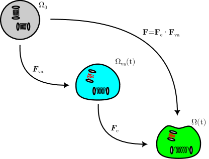
Figure 2: Multiplicative decomposition of the deformation gradient for viscoelastic active fluids.

We choose the decomposition as $\underaccent{\hskip 0.70004pt\approx}{\boldsymbol{\mathbf{F}}}=\underaccent{\hskip 0.70004pt\approx}{\boldsymbol{\mathbf{F}}}_{\!\mathrm{e}}\underaccent{\hskip 0.70004pt\approx}{\boldsymbol{\mathbf{F}}}_{\!\mathrm{va}}$, illustrated in Fig. 2, where $\underaccent{\hskip 0.70004pt\approx}{\boldsymbol{\mathbf{F}}}_{\!\mathrm{e}}$ corresponds to elastic deformations of the microstructure, and $\underaccent{\hskip 0.70004pt\approx}{\boldsymbol{\mathbf{F}}}_{\!\mathrm{va}}$ corresponds to both viscous-like deformations due to the relaxation of the elastic microstructure and active deformation due to a chemically-driven growth or contraction of the microstructure.

We now aim at writing the free energy in terms of the active deformation tensor in addition to the elastic strain, $\varphi_{\text{mult}}(\underaccent{\hskip 0.70004pt\approx}{\boldsymbol{\mathbf{F}}}_{\!\mathrm{e}},\underaccent{\hskip 0.70004pt\approx}{\boldsymbol{\mathbf{F}}}_{\!\mathrm{va}})=\varphi(\underaccent{\hskip 0.70004pt\approx}{\boldsymbol{\mathbf{A}}},\xi_{\mathrm{a}})$ as defined in Eq. (16). Thus $\underaccent{\hskip 0.70004pt\approx}{\boldsymbol{\mathbf{F}}}_{\!\mathrm{e}}$ should be related to $\underaccent{\hskip 0.70004pt\approx}{\boldsymbol{\mathbf{A}}}$ and $\underaccent{\hskip 0.70004pt\approx}{\boldsymbol{\mathbf{F}}}_{\!\mathrm{va}}$ with $\xi_{\mathrm{a}}$.

The tensor $\underaccent{\hskip 0.70004pt\approx}{\boldsymbol{\mathbf{A}}}$ is by construction symmetric and positive semidefinite (and positive definite as long as $\mathrm{Supp}\,\psi_{\mathrm{b}}$ has nonzero measure, which can be ensured by smooth initial conditions and the affine or diffusive nature of the fluxes in Eq. (6)). Thus Cholesky factorisation guarantees the existence of an upper triangular tensor $\underaccent{\hskip 0.70004pt\approx}{\boldsymbol{\mathbf{U}}}$ such that $\underaccent{\hskip 0.70004pt\approx}{\boldsymbol{\mathbf{A}}}=\underaccent{\hskip 0.70004pt\approx}{\boldsymbol{\mathbf{U}}}\cdot^{\!\mathsf{T}}\underaccent{\hskip 0.70004pt\approx}{\boldsymbol{\mathbf{U}}}=\underaccent{\hskip 0.70004pt\approx}{\boldsymbol{\mathbf{U}}}^{\!\mathsf{T}}\cdot\underaccent{\hskip 0.70004pt\approx}{\boldsymbol{\mathbf{O}}}^{\!\mathsf{T}}\cdot\underaccent{\hskip 0.70004pt\approx}{\boldsymbol{\mathbf{O}}}\cdot\underaccent{\hskip 0.70004pt\approx}{\boldsymbol{\mathbf{U}}}$ with $\underaccent{\hskip 0.70004pt\approx}{\boldsymbol{\mathbf{O}}}$ an orthogonal matrix. Thus we can set $\underaccent{\hskip 0.70004pt\approx}{\boldsymbol{\mathbf{F}}}_{\!\mathrm{e}}$ so that $\underaccent{\hskip 0.70004pt\approx}{\boldsymbol{\mathbf{A}}}$ is either $\alpha\underaccent{\hskip 0.70004pt\approx}{\boldsymbol{\mathbf{F}}}_{\!\mathrm{e}}^{\!\mathsf{T}}\cdot\underaccent{\hskip 0.70004pt\approx}{\boldsymbol{\mathbf{F}}}_{\!\mathrm{e}}$ or $\alpha\underaccent{\hskip 0.70004pt\approx}{\boldsymbol{\mathbf{F}}}_{\!\mathrm{e}}\cdot\underaccent{\hskip 0.70004pt\approx}{\boldsymbol{\mathbf{F}}}_{\!\mathrm{e}}^{\!\mathsf{T}}$, with $\alpha$ a constant, imposing that the upper diagonal matrix in the QR-decomposition of $\underaccent{\hskip 0.70004pt\approx}{\boldsymbol{\mathbf{F}}}_{\!\mathrm{e}}$ is $\underaccent{\hskip 0.70004pt\approx}{\boldsymbol{\mathbf{U}}}$. Since in both choices, the invariants $\underaccent{\hskip 0.70004pt\approx}{\boldsymbol{\mathbf{F}}}_{\!\mathrm{e}}^{\!\mathsf{T}}\cdot\underaccent{\hskip 0.70004pt\approx}{\boldsymbol{\mathbf{F}}}_{\!\mathrm{e}}:\underaccent{\hskip 0.70004pt\approx}{\boldsymbol{\mathbf{I}}}=\underaccent{\hskip 0.70004pt\approx}{\boldsymbol{\mathbf{F}}}_{\!\mathrm{e}}\cdot\underaccent{\hskip 0.70004pt\approx}{\boldsymbol{\mathbf{F}}}_{\!\mathrm{e}}^{\!\mathsf{T}}:\underaccent{\hskip 0.70004pt\approx}{\boldsymbol{\mathbf{I}}}=\underaccent{\hskip 0.70004pt\approx}{\boldsymbol{\mathbf{F}}}_{\!\mathrm{e}}:\underaccent{\hskip 0.70004pt\approx}{\boldsymbol{\mathbf{F}}}_{\!\mathrm{e}}$ are identical, we make our choice in order to be able to define the corresponding $\underaccent{\hskip 0.70004pt\approx}{\boldsymbol{\mathbf{F}}}_{\!\mathrm{va}}$ conveniently. Like Califano-Ciambella.2023.1, we remark that the (Eulerian) left Cauchy–Green tensor $\underaccent{\hskip 0.70004pt\approx}{\boldsymbol{\mathbf{B}}}=\underaccent{\hskip 0.70004pt\approx}{\boldsymbol{\mathbf{F}}}\cdot\underaccent{\hskip 0.70004pt\approx}{\boldsymbol{\mathbf{F}}}^{\!\mathsf{T}}$ is such that $\dot{\underaccent{\hskip 0.70004pt\approx}{\boldsymbol{\mathbf{B}}}}\vphantom{\underaccent{\hskip 0.70004pt\approx}{\boldsymbol{\mathbf{B}}}}=\underaccent{\approx}{\boldsymbol{{{\ell}}}}\cdot\underaccent{\hskip 0.70004pt\approx}{\boldsymbol{\mathbf{B}}}+\underaccent{\hskip 0.70004pt\approx}{\boldsymbol{\mathbf{B}}}\cdot\underaccent{\approx}{\boldsymbol{{{\ell}}}}\,^{\!\mathsf{T}}$ and thus, that its upper convected derivative is zero, which guides us to choose $\underaccent{\hskip 0.70004pt\approx}{\boldsymbol{\mathbf{F}}}_{\!\mathrm{e}}$ such that $\underaccent{\hskip 0.70004pt\approx}{\boldsymbol{\mathbf{F}}}_{\!\mathrm{e}}\cdot\underaccent{\hskip 0.70004pt\approx}{\boldsymbol{\mathbf{F}}}_{\!\mathrm{e}}^{\!\mathsf{T}}=\alpha\underaccent{\hskip 0.70004pt\approx}{\boldsymbol{\mathbf{A}}}$.

As a result, $\underaccent{\hskip 0.70004pt\approx}{\boldsymbol{\mathbf{A}}}=\underaccent{\hskip 0.70004pt\approx}{\boldsymbol{\mathbf{F}}}\cdot\underaccent{\hskip 0.70004pt\approx}{\boldsymbol{\mathbf{C}}}_{\!\mathrm{va}}^{-1}\cdot\underaccent{\hskip 0.70004pt\approx}{\boldsymbol{\mathbf{F}}}^{\!\mathsf{T}}$ with $\underaccent{\hskip 0.70004pt\approx}{\boldsymbol{\mathbf{C}}}_{\!\mathrm{va}}^{-1}=(\underaccent{\hskip 0.70004pt\approx}{\boldsymbol{\mathbf{F}}}_{\!\mathrm{v}}\cdot\underaccent{\hskip 0.70004pt\approx}{\boldsymbol{\mathbf{F}}}_{\!\mathrm{a}})^{-1}\cdot(\underaccent{\hskip 0.70004pt\approx}{\boldsymbol{\mathbf{F}}}_{\!\mathrm{v}}\cdot\underaccent{\hskip 0.70004pt\approx}{\boldsymbol{\mathbf{F}}}_{\!\mathrm{a}})^{-\!\mathsf{T}}$, and by derivation

$$\accentset{\triangledown}{\underaccent{\hskip 0.70004pt\approx}{\boldsymbol{\mathbf{A}}}}=\dot{}\underaccent{\hskip 0.70004pt\approx}{\boldsymbol{\mathbf{A}}}-\underaccent{\approx}{\boldsymbol{{{\ell}}}}\cdot\underaccent{\hskip 0.70004pt\approx}{\boldsymbol{\mathbf{A}}}+\underaccent{\hskip 0.70004pt\approx}{\boldsymbol{\mathbf{A}}}\cdot\underaccent{\approx}{\boldsymbol{{{\ell}}}}^{\!\mathsf{T}}=\underaccent{\hskip 0.70004pt\approx}{\boldsymbol{\mathbf{F}}}\frac{\mathrm{d}\underaccent{\hskip 0.70004pt\approx}{\boldsymbol{\mathbf{C}}}_{\!\mathrm{va}}^{-1}}{\mathrm{d}t}\cdot\underaccent{\hskip 0.70004pt\approx}{\boldsymbol{\mathbf{F}}}^{\!\mathsf{T}}$$

which allows to use Eq. (13) set the dynamics of $\underaccent{\hskip 0.70004pt\approx}{\boldsymbol{\mathbf{C}}}_{\!\mathrm{va}}^{-1}$,

$$k_{\mathrm{u}}^{-1}\underaccent{\hskip 0.70004pt\approx}{\boldsymbol{\mathbf{F}}}\cdot\frac{\mathrm{d}\underaccent{\hskip 0.70004pt\approx}{\boldsymbol{\mathbf{C}}}_{\!\mathrm{va}}^{-1}}{\mathrm{d}t}\cdot\underaccent{\hskip 0.70004pt\approx}{\boldsymbol{\mathbf{F}}}^{\!\mathsf{T}}=-\underaccent{\hskip 0.70004pt\approx}{\boldsymbol{\mathbf{F}}}\cdot\underaccent{\hskip 0.70004pt\approx}{\boldsymbol{\mathbf{C}}}_{\!\mathrm{va}}^{-1}\cdot\underaccent{\hskip 0.70004pt\approx}{\boldsymbol{\mathbf{F}}}^{\!\mathsf{T}}+\underaccent{\hskip 0.70004pt\approx}{\boldsymbol{\mathbf{A}}}_{0}+\underaccent{\hskip 0.70004pt\approx}{\boldsymbol{\mathbf{A}}}_{\mathrm{a}}$$

which yields, since $\underaccent{\hskip 0.70004pt\approx}{\boldsymbol{\mathbf{A}}}_{0}=a_{0}\beta^{-2}\underaccent{\hskip 0.70004pt\approx}{\boldsymbol{\mathbf{I}}}$,

$$k_{\mathrm{u}}^{-1}\frac{\mathrm{d}\underaccent{\hskip 0.70004pt\approx}{\boldsymbol{\mathbf{C}}}_{\!\mathrm{va}}^{-1}}{\mathrm{d}t}=-\underaccent{\hskip 0.70004pt\approx}{\boldsymbol{\mathbf{C}}}_{\!\mathrm{va}}^{-1}+\alpha a_{0}\underaccent{\hskip 0.70004pt\approx}{\boldsymbol{\mathbf{C}}}^{-1}+\underaccent{\hskip 0.70004pt\approx}{\boldsymbol{\mathbf{F}}}^{-1}\cdot\underaccent{\hskip 0.70004pt\approx}{\boldsymbol{\mathbf{A}}}_{\mathrm{a}}\cdot\underaccent{\hskip 0.70004pt\approx}{\boldsymbol{\mathbf{F}}}^{-\!\mathsf{T}}.$$ (19)

In the permanent regime and in the absence of active stresses $\underaccent{\hskip 0.70004pt\approx}{\boldsymbol{\mathbf{A}}}_{\mathrm{a}}$, elastic strains relax and thus $\underaccent{\hskip 0.70004pt\approx}{\boldsymbol{\mathbf{C}}}_{\!\mathrm{va}}^{-1}=\underaccent{\hskip 0.70004pt\approx}{\boldsymbol{\mathbf{C}}}^{-1}$. We thus set $\alpha=\beta^{2}a_{0}^{-1}=2\beta^{2}$ using this limit behaviour.

In summary, the model of Section 2.6 can now be rewritten using the multiplicative decomposition. Given $\underaccent{\hskip 0.70004pt\approx}{\boldsymbol{\mathbf{A}}}_{\mathrm{a}},G,\mu,k_{\mathrm{u}}$, find $(\underaccent{\hskip 0.70004pt\approx}{\boldsymbol{\mathbf{F}}}_{\!\mathrm{va}},\underaccent{\hskip 0.70004pt\approx}{\boldsymbol{\mathbf{F}}}_{\!\mathrm{e}},p)$ such that:

$$k_{\mathrm{u}}^{-1}\frac{\mathrm{d}\underaccent{\hskip 0.70004pt\approx}{\boldsymbol{\mathbf{C}}}_{\!\mathrm{va}}^{-1}}{\mathrm{d}t} =-\underaccent{\hskip 0.70004pt\approx}{\boldsymbol{\mathbf{C}}}_{\!\mathrm{va}}^{-1}+\underaccent{\hskip 0.70004pt\approx}{\boldsymbol{\mathbf{F}}}^{-1}\underaccent{\hskip 0.70004pt\approx}{\boldsymbol{\mathbf{F}}}^{-\!\mathsf{T}}+\underaccent{\hskip 0.70004pt\approx}{\boldsymbol{\mathbf{F}}}^{-1}\cdot\underaccent{\hskip 0.70004pt\approx}{\boldsymbol{\mathbf{A}}}_{\mathrm{a}}\cdot\underaccent{\hskip 0.70004pt\approx}{\boldsymbol{\mathbf{F}}}^{-\!\mathsf{T}},$$ (20)

$$\underaccent{\sim}{\boldsymbol{{\nabla}}}_{\!{\boldsymbol{{x}}}}\cdot\underaccent{\hskip 0.70004pt\approx}{\boldsymbol{\mathbf{\sigma}}}-\underaccent{\sim}{\boldsymbol{{\nabla}}}_{\!{\boldsymbol{{x}}}}p =\underaccent{\sim}{\boldsymbol{{0}}},$$ (21)

$$\det\underaccent{\hskip 0.70004pt\approx}{\boldsymbol{\mathbf{F}}} =1,$$ (22)

with:

$$\underaccent{\hskip 0.70004pt\approx}{\boldsymbol{\mathbf{\sigma}}} =2G(\underaccent{\hskip 0.70004pt\approx}{\boldsymbol{\mathbf{F}}}_{\!\mathrm{e}}\cdot\underaccent{\hskip 0.70004pt\approx}{\boldsymbol{\mathbf{F}}}_{\!\mathrm{e}}^{\!\mathsf{T}}-\underaccent{\hskip 0.70004pt\approx}{\boldsymbol{\mathbf{I}}})+\mu(\underaccent{\approx}{\boldsymbol{{{\ell}}}}+\underaccent{\approx}{\boldsymbol{{{\ell}}}}\,^{\!\mathsf{T}}),$$ (23)

$$\underaccent{\hskip 0.70004pt\approx}{\boldsymbol{\mathbf{F}}} =\underaccent{\hskip 0.70004pt\approx}{\boldsymbol{\mathbf{F}}}_{\!\mathrm{e}}\underaccent{\hskip 0.70004pt\approx}{\boldsymbol{\mathbf{F}}}_{\!\mathrm{va}},$$ (24)

$$\underaccent{\hskip 0.70004pt\approx}{\boldsymbol{\mathbf{C}}}_{\!\mathrm{va}}^{-1} =\underaccent{\hskip 0.70004pt\approx}{\boldsymbol{\mathbf{F}}}_{\!\mathrm{va}}^{-1}\underaccent{\hskip 0.70004pt\approx}{\boldsymbol{\mathbf{F}}}_{\!\mathrm{va}}^{-\!\mathsf{T}},$$ (25)

$$\underaccent{\approx}{\boldsymbol{{{\ell}}}} =\dot{\underaccent{\hskip 0.70004pt\approx}{\boldsymbol{\mathbf{F}}}}\vphantom{\underaccent{\hskip 0.70004pt\approx}{\boldsymbol{\mathbf{F}}}}\underaccent{\hskip 0.70004pt\approx}{\boldsymbol{\mathbf{F}}}^{-1},$$ (26)

subject to an initial condition on $\underaccent{\hskip 0.70004pt\approx}{\boldsymbol{\mathbf{C}}}_{\!\mathrm{va}}$ and boundary conditions on $(\underaccent{\hskip 0.70004pt\approx}{\boldsymbol{\mathbf{\sigma}}}-p\underaccent{\hskip 0.70004pt\approx}{\boldsymbol{\mathbf{I}}})\cdot\underaccent{\sim}{\boldsymbol{{n}}}$.

4 Example application: active viscoelastic beam on an elastic substrate

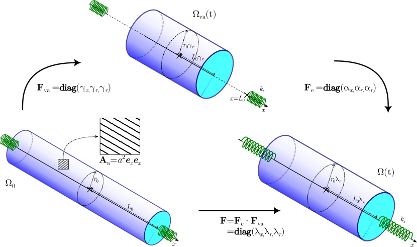
Figure 3: Illustration of a uniaxially contractile beam interacting with an elastic environment. The initial configuration $\Omega_{0}$ of the beam is before the active strain $\underaccent{\hskip 0.70004pt\approx}{\boldsymbol{\mathbf{A}}}_{\mathrm{a}}$ has been applied, and is chosen here at equilibrium with the external springs. The visco-active deformation $\underaccent{\hskip 0.70004pt\approx}{\boldsymbol{\mathbf{F}}}_{\!\mathrm{va}}(t)$ gives the intermediate virtual configuration $\Omega_{\mathrm{va}}(t)$, a configuration which is not compatible with the external forces and does not obey incompressibility. The elastic deformation $\underaccent{\hskip 0.70004pt\approx}{\boldsymbol{\mathbf{F}}}_{\!\mathrm{e}}(t)$ restores both of these requirements in the current configuration $\Omega(t)$. The time evolution of $\underaccent{\hskip 0.70004pt\approx}{\boldsymbol{\mathbf{F}}}_{\!\mathrm{va}}(t)$ is prescribed by the relaxation dynamics of the microstructure $\underaccent{\hskip 0.70004pt\approx}{\boldsymbol{\mathbf{A}}}$ towards a state where the elastic stress is equal to the active stress, $\underaccent{\hskip 0.70004pt\approx}{\boldsymbol{\mathbf{\sigma}}}(t_{\mathrm{eq}})=2\nu\kappa(\underaccent{\hskip 0.70004pt\approx}{\boldsymbol{\mathbf{A}}}(t_{\mathrm{eq}})-\underaccent{\hskip 0.70004pt\approx}{\boldsymbol{\mathbf{A}}}_{0})=2\nu\kappa\underaccent{\hskip 0.70004pt\approx}{\boldsymbol{\mathbf{A}}}_{\mathrm{a}}=\underaccent{\hskip 0.70004pt\approx}{\boldsymbol{\mathbf{\sigma}}}_{\mathrm{a}}$.

We model a slender active viscoelastic beam, which can for example represent a stress fibre in a cell with adhesion at its ends only Katoh et al., (1998). We neglect the liquid bath viscosities $\mu=\mu_{b}=0$. It initially spans the distance from $(-L_{0},0,0)^{\!\mathsf{T}}$ to $(L_{0},0,0)^{\!\mathsf{T}}$ and has radius $r_{0}$. With this geometry and restricting load to the longitudinal direction only, the deformation tensors are diagonal tensors and we write $\underaccent{\hskip 0.70004pt\approx}{\boldsymbol{\mathbf{F}}}_{\!\mathrm{e}}=\operatorname{\mathbf{diag}}(\alpha_{x},\alpha_{r},\alpha_{r})$, $\underaccent{\hskip 0.70004pt\approx}{\boldsymbol{\mathbf{F}}}_{\!\mathrm{va}}=\operatorname{\mathbf{diag}}(\gamma_{x},\gamma_{r},\gamma_{r})$ and $\underaccent{\hskip 0.70004pt\approx}{\boldsymbol{\mathbf{F}}}=\operatorname{\mathbf{diag}}(\lambda_{x},\lambda_{r},\lambda_{r})=\operatorname{\mathbf{diag}}(\gamma_{x}\alpha_{x},\gamma_{r}\alpha_{r},\gamma_{r}\alpha_{r})$. We assume that the chains within the beam are all oriented along the main axis $x$ of the beam, leading to $\langle\underaccent{\hskip 0.70004pt\approx}{\boldsymbol{\mathbf{Q}}}\rangle_{\mathrm{b}}=\underaccent{\sim}{\boldsymbol{{e}}}_{x}\underaccent{\sim}{\boldsymbol{{e}}}_{x}$ and $\underaccent{\hskip 0.70004pt\approx}{\boldsymbol{\mathbf{A}}}_{\mathrm{a}}=a^{2}\underaccent{\sim}{\boldsymbol{{e}}}_{x}\underaccent{\sim}{\boldsymbol{{e}}}_{x}$. The external forces are supposed to be zero along the beam itself (no friction), except for tractions $\pm F\underaccent{\sim}{\boldsymbol{{e}}}_{x}=\pm 2k_{s}L_{0}(1-\lambda_{x})\underaccent{\sim}{\boldsymbol{{e}}}_{x}$ applied at each end $x=\pm L_{0}$ of the beam and which correspond to the elastic resistance to the deformation of the substrate which behaves as a spring of stiffness $k_{s}$. We define $E_{s}=k_{s}L_{0}/(\pi r_{0}^{2})$.

Taking the pressure to be a Lagrange multiplier that imposes incompressibility, we have the equilibrium equations:

$$2G(\alpha_{x}^{2}-1)-p =E_{s}(1-\lambda_{x})\lambda_{r}^{-2}$$ (27)

$$2G(\alpha_{r}^{2}-1)-p =0$$ (28)

$$\lambda_{r}^{2}\lambda_{x} =1$$ (29)

Thus, subtracting the $r$ equation to the $x$ one to eliminate pressure, and using the incompressibility condition,

$$\lambda_{x}^{2}-\lambda_{x}-\frac{2G}{E_{s}}(\alpha_{x}^{2}-\alpha_{r}^{2})=0$$

From Eq. (19), we have:

$$2\tau\dot{\gamma}_{x} =(\alpha_{x}^{2}-1-a^{2})\alpha_{x}^{-2}\gamma_{x}$$ (30)

$$2\tau\dot{\gamma}_{r} =(\alpha_{r}^{2}-1)\alpha_{r}^{-2}\gamma_{r}$$ (31)

Since $\gamma_{i}>0$, the only admissible long times solution is $\alpha_{x}^{2}=1+a^{2}$ and $\alpha_{r}=1$. Thus the admissible solution is $\lambda_{x}=\frac{1}{2}(1+\sqrt{1+8Ga^{2}/E_{s}})$. It is an incompressibility effect that the beam cannot be shorter than $L_{0}/2$: indeed, due to the broadening section of the beam, the external traction would then decrease with increasing deformation.

The relevance of this model for actomyosin-based systems is discussed by Étienne et al., (2015), where we also find that a viscoelastic liquid material with an internal active stress adapts in length to the external stiffness $E_{s}$.

5 Conclusions

In this paper, we derive the specific shape and dependences on microscopic processes of active terms that are present in linearisations of the active gel theory Kruse et al., (2005) while ensuring that they are consistent with thermodynamical requirements. Rather than start from the free energy of nematic liquid crystals Kruse et al., (2004, 2005), where no stretching of the microstructure is possible, we start from the entropic elasticity of Gaussian chains that model the actin filaments between two crosslinks. This possibility of stretching the filaments is at the origin of the specific shape of the objective derivative in the constitutive equation Hinch and Harlen, (2021), whose nonlinearities are negligible only in the purely viscous limit. Thus, whenever the timescale of the process at play is comparable to the relaxation time, the correct form of the constitutive equation is an upper-convected viscoelastic liquid material law. The model we derive here has a single relaxation time, however similar extensions as those of the Lodge network model (Larson,, 1999, p. 120) can be relevant for biopolymers Broedersz et al., (2010), and could allow to fit the fractional exponents observed in experiments Trepat et al., (2008); Bonfanti et al., (2020). The simplest of these laws, when only one relaxation time is present—either due to the material itself or because the timescale of the process is comparable but larger than the largest relaxation time—is the upper-convected Maxwell equation.

A link is explicitely made between the microscopic scale behaviour of molecular motors and the continuum scale active stress. Compared to a previous such attempt Étienne et al., (2015), we are now able to define conditions for which microscopic scale kinetics are thermodynamically admissible. When motors are assumed to walk randomly along actin filaments, we recapitulate the results from Étienne et al., (2015), reaching an anisotropic contractility which scales as the square of the length of the typical step performed by a power-stroke of the myosin. We can also envision a case where motors walk processively along polar filaments. The resulting shape of the anisotropic contractility remains similar as in the above case, but with a linear dependence in the step size and thus a higher efficiency. We show that this active contribution appears as an offset of the isotropic rest configuration of the microstructure to a new configuration with prestrained microstucture configuration.

Active biopolymer networks encompass both subcellular structures such as the actomyosin and tissue scale fibrous tissue Erlich et al., (2022). Contractility of actomyosin is also felt in cellularised tissue like epithelia Khalilgharibi et al., (2016); Erlich et al., (2022) which are often simulated with similar continuum models Dicko et al., (2017); Wyatt et al., (2020). For those it is not appropriate to use elastic chains as the microstructure, however when considering the kinetics of cell deformation and neighbour exchanges, models of the same shape as the present model are found, including the upper-convected objective derivative Tlili et al., (2015); Ishihara et al., (2017); Bandil and Vernerey, (2023). A possible direction for these materials is to consider a non-Hookean elasticity of the microstructure, e.g. with a finite extensibility approach (Larson,, 1999, p. 142).

Viscoelastic liquids lead to mathematical problems notoriously difficult to solve analytically or numerically, and the set of equations in Section 2.6 can prove challenging to solve for complex geometries. In addition, biopolymer networks such as actomyosin often form thin shell-like structures Erlich et al., (2022), which turns the problem into a moving domain partial differential system. We propose to use the formalism of multiplicative strain decomposition, as is done for plasticity or morphoelastic descriptions of growth Lubarda, (2004) in order to simplify the resolution procedure.

Appendix A Dynamics of the unbound chains

In order to give the term of order $\frac{\zeta k_{\mathrm{u}}}{\kappa}$ in Eq. (5b), we expand $\psi_{\mathrm{u}}$ as:

$$\psi_{\mathrm{u}}(\underaccent{\sim}{\boldsymbol{{r}}},t)=a_{\mathrm{u}}\left(\psi_{0}(\underaccent{\sim}{\boldsymbol{{r}}})+\frac{\zeta k_{\mathrm{u}}}{\kappa}\psi_{\mathrm{u}}^{\prime}(\underaccent{\sim}{\boldsymbol{{r}}},t)\right).$$

When $\psi_{\mathrm{u}}$ deviates from $a_{\mathrm{u}}\psi_{0}$, the force resultant balanced by the drag force is:

$$\underaccent{\sim}{\boldsymbol{{F}}}_{s}(\underaccent{\sim}{\boldsymbol{{r}}})+\underaccent{\sim}{\boldsymbol{{F}}}_{b}(\underaccent{\sim}{\boldsymbol{{r}}},\psi_{\mathrm{u}}) =-k_{B}T\frac{\zeta k_{\mathrm{u}}}{\kappa}\underaccent{\sim}{\boldsymbol{{\nabla}}}_{\!{\boldsymbol{{r}}}}\left(\frac{\psi_{\mathrm{u}}^{\prime}}{\psi_{0}}\right)+O\left(\frac{(\zeta k_{\mathrm{u}})^{2}\beta}{\kappa}\right)$$

$$=-\frac{\zeta k_{\mathrm{u}}}{\kappa\psi_{0}}\left(k_{B}T\underaccent{\sim}{\boldsymbol{{\nabla}}}_{\!{\boldsymbol{{r}}}}\psi_{\mathrm{u}}^{\prime}+\kappa\psi_{\mathrm{u}}^{\prime}\underaccent{\sim}{\boldsymbol{{r}}}\right)+O\left(\frac{(\zeta k_{\mathrm{u}})^{2}\beta}{\kappa}\right)$$

and, to the first order, Eq. (5b) gives:

$$k_{\mathrm{u}}a_{\mathrm{u}}\underaccent{\sim}{\boldsymbol{{\nabla}}}_{\!{\boldsymbol{{r}}}}\cdot\left(\psi_{\mathrm{u}}^{\prime}\underaccent{\sim}{\boldsymbol{{r}}}+\frac{k_{B}T}{\kappa}\underaccent{\sim}{\boldsymbol{{\nabla}}}_{\!{\boldsymbol{{r}}}}\psi_{\mathrm{u}}^{\prime}\right) =a_{\mathrm{u}}\underaccent{\sim}{\boldsymbol{{\nabla}}}_{\!{\boldsymbol{{r}}}}\cdot(\psi_{0}\underaccent{\sim}{\boldsymbol{{r}}}\cdot\underaccent{\sim}{\boldsymbol{{\nabla}}}_{\!{\boldsymbol{{x}}}}\underaccent{\sim}{\boldsymbol{{v}}})-k_{\mathrm{u}}\mathcal{K}_{0}(\psi_{\mathrm{b}})+O\left(\frac{\zeta k_{\mathrm{u}}^{2}}{\kappa}\right)$$ (32)

Thus there is a fast relaxation of the unbound chains to a distribution which varies in time only inasmuch as $k_{\mathrm{u}}\mathcal{K}_{0}(\psi_{\mathrm{b}}):=k_{\mathrm{u}}\mathcal{K}_{u}(\psi_{\mathrm{b}}(t),a_{\mathrm{u}}\psi_{0})$ does.

Appendix B Diffusive molecular motors

In Section 2.5 we assume that molecular motors can sense a directionality in the network and follow the oriented vector $\underaccent{\sim}{\boldsymbol{{r}}}$. This corresponds to the behaviour of myosin minifilaments on actin networks, however this may not be the case of all contractile biopolymer networks. Starting again from Eqs. (15), it is possible to construct another vectorial reaction coefficient based on the gradient of $\psi_{\mathrm{b}}$, i.e. for any orientation tensor $\underaccent{\hskip 0.70004pt\approx}{\boldsymbol{\mathbf{q}}}$,

$$\lambda_{12}^{\text{diff}} =-\frac{k_{\mathrm{a}}^{\text{diff}}\theta^{\text{diff}}}{\kappa}\underaccent{\hskip 0.70004pt\approx}{\boldsymbol{\mathbf{q}}}\underaccent{\sim}{\boldsymbol{{\nabla}}}_{\!{\boldsymbol{{r}}}}\log\psi_{\mathrm{b}}, \underaccent{\sim}{\boldsymbol{{j}}}_{\mathrm{\!a}}^{\text{diff}} =-\frac{k_{\mathrm{a}}^{\text{diff}}\theta^{\text{diff}}\Delta\mu}{\kappa}\underaccent{\hskip 0.70004pt\approx}{\boldsymbol{\mathbf{q}}}\underaccent{\sim}{\boldsymbol{{\nabla}}}_{\!{\boldsymbol{{r}}}}\log\psi_{\mathrm{b}},$$

$$\dot{\xi}_{\mathrm{a}}^{\text{diff}} =-{2k_{\mathrm{a}}^{\text{diff}}}\underaccent{\sim}{\boldsymbol{{r}}}\cdot\underaccent{\hskip 0.70004pt\approx}{\boldsymbol{\mathbf{q}}}\underaccent{\sim}{\boldsymbol{{\nabla}}}_{\!{\boldsymbol{{r}}}}\log\psi_{\mathrm{b}}+\lambda_{22}\Delta\mu.$$

For simplicity we have taken $k_{\mathrm{s}}=0$. In Étienne et al., (2015), we argue that the resulting diffusion term in Eq. (6) must scale with the square of the size of the steps $\ell_{\mathrm{m}}$ that the molecular motors perform on the strands, thus $\theta^{\text{diff}}=\ell_{\mathrm{m}}^{2}\beta^{2}$

If $\underaccent{\hskip 0.70004pt\approx}{\boldsymbol{\mathbf{q}}}=\underaccent{\hskip 0.70004pt\approx}{\boldsymbol{\mathbf{I}}}$, since $\langle-\underaccent{\sim}{\boldsymbol{{r}}}\underaccent{\sim}{\boldsymbol{{\nabla}}}_{\!{\boldsymbol{{r}}}}\log\psi_{\mathrm{b}}\rangle_{\mathrm{b}}=\underaccent{\hskip 0.70004pt\approx}{\boldsymbol{\mathbf{I}}}$, the average rate of advancement of the reaction is $\langle\dot{\xi}_{\mathrm{a}}^{\text{diff}}\rangle_{\mathrm{b}}=2k_{\mathrm{a}}^{\text{diff}}+\lambda_{22}$ and is thus independent of the mechanical stress. The microstructure active deformation tensor and the active stress in this case are:

$$\underaccent{\hskip 0.70004pt\approx}{\boldsymbol{\mathbf{A}}}_{\mathrm{a}} =\frac{2k_{\mathrm{a}}^{\text{diff}}\ell_{\mathrm{m}}^{2}\beta^{2}\Delta\mu}{k_{\mathrm{u}}\kappa}\underaccent{\hskip 0.70004pt\approx}{\boldsymbol{\mathbf{I}}}, \underaccent{\hskip 0.70004pt\approx}{\boldsymbol{\mathbf{\sigma}}}_{\mathrm{a}} ={2\nu\Delta\mu\ell_{\mathrm{m}}^{2}\beta^{2}k_{\mathrm{a}}^{\text{diff}}}\frac{k_{\mathrm{a}}}{k_{\mathrm{u}}}\underaccent{\hskip 0.70004pt\approx}{\boldsymbol{\mathbf{I}}}.$$

However the lack of alignment of the velocity $\underaccent{\sim}{\boldsymbol{{j}}}_{\mathrm{\!a}}$ with the microstructure is difficult to interpret. Following Étienne et al., (2015), it is also possible to take $\underaccent{\hskip 0.70004pt\approx}{\boldsymbol{\mathbf{q}}}=\underaccent{\hskip 0.70004pt\approx}{\boldsymbol{\mathbf{Q}}}$, which means that the diffusive-like behaviour of the molecular motors takes place along the direction of the strands $\underaccent{\sim}{\boldsymbol{{r}}}/|\underaccent{\sim}{\boldsymbol{{r}}}|$. Thanks to the property $\langle-\underaccent{\sim}{\boldsymbol{{r}}}\underaccent{\hskip 0.70004pt\approx}{\boldsymbol{\mathbf{Q}}}\underaccent{\sim}{\boldsymbol{{\nabla}}}_{\!{\boldsymbol{{r}}}}\log\psi_{\mathrm{b}}\rangle_{\mathrm{b}}=\langle\underaccent{\hskip 0.70004pt\approx}{\boldsymbol{\mathbf{Q}}}\rangle_{\mathrm{b}}$, as above, and to the fact that $\operatorname{tr}\underaccent{\hskip 0.70004pt\approx}{\boldsymbol{\mathbf{Q}}}=1$, we have $\langle\dot{\xi}_{\mathrm{a}}^{\text{diff}}\rangle_{\mathrm{b}}=2k_{\mathrm{a}}^{\text{diff}}+\lambda_{22}$ and is thus independent of the mechanical stress. The microstructure active deformation tensor and the active stress are then:

$$\underaccent{\hskip 0.70004pt\approx}{\boldsymbol{\mathbf{A}}}_{\mathrm{a}} =\frac{2k_{\mathrm{a}}\ell_{\mathrm{m}}^{2}\beta^{2}\Delta\mu}{k_{\mathrm{u}}\kappa}\langle\underaccent{\hskip 0.70004pt\approx}{\boldsymbol{\mathbf{Q}}}\rangle_{\mathrm{b}}, \underaccent{\hskip 0.70004pt\approx}{\boldsymbol{\mathbf{\sigma}}}_{\mathrm{a}} ={2\nu\ell_{\mathrm{m}}^{2}\beta^{2}\Delta\mu}\frac{k_{\mathrm{a}}}{k_{\mathrm{u}}}\langle\underaccent{\hskip 0.70004pt\approx}{\boldsymbol{\mathbf{Q}}}\rangle_{\mathrm{b}}.$$

Thus we find that the “diffusive” and “processive” types of reactive flux $\underaccent{\sim}{\boldsymbol{{j}}}_{\mathrm{\!a}}$ lead to expressions of the active stress which differ only by the factor $\ell_{\mathrm{m}}^{2}\beta/\ell_{\mathrm{a}}$. The distance $\ell_{\mathrm{a}}$ over which a myosin motor is processive can be expected to be much greater than the Kuhn length $\beta^{-1}$ and motor steps $\ell_{\mathrm{m}}^{2}$, thus the processive behaviour is much more efficient.

References

• Alrashdi and Giusteri, (2024) Alrashdi and Giusteri (2024). Evolution of local relaxed states and the modelling of viscoelastic fluids. arXiv.
• Bandil and Vernerey, (2023) Bandil, P. and Vernerey, F. J. (2023). Continuum theory for confluent cell monolayers: Interplay between cell growth, division, and intercalation. Journal of the Mechanics and Physics of Solids, 181:105443.
• Bergou et al., (2010) Bergou, M., Audoly, B., Vouga, E., Wardetzky, M., and Grinspun, E. (2010). Discrete viscous threads. ACM Transactions on graphics (TOG), 29:1–10.
• Bertinetti et al., (2015) Bertinetti, L., Masic, A., Schuetz, R., Barbetta, A., Seidt, B., Wagermaier, W., and Fratzl, P. (2015). Osmotically driven tensile stress in collagen-based mineralized tissues. Journal of the Mechanical Behavior of Biomedical Materials, 52:14–21.
• Bird et al., (1987) Bird, R., Armstrong, R. C., and Hassager, O. (1987). Dynamics of polymeric liquids. Volume 2. Kinetic theory. Wiley, New-York.
• Bonfanti et al., (2020) Bonfanti, A., Fouchard, J., Khalilgharibi, N., Charras, G., and Kabla, A. (2020). A unified rheological model for cells and cellularised materials. R. Soc. open sci., 7:190920.
• Bray and White, (1988) Bray, D. and White, J. G. (1988). Cortical flow in animal cells. Science Mag., 239:883–888.
• Broedersz et al., (2010) Broedersz, C. P., Depken, M., Yao, N. Y., Pollak, M. R., Weitz, D. A., and MacKintosh, F. C. (2010). Cross-link governed dynamics of biopolymer networks. Phys. Rev. Lett., 105:238101.
• Caruel and Truskinovsky, (2018) Caruel, M. and Truskinovsky, L. (2018). Physics of muscle contraction. Rep. Prog. Phys., 81:036602.
• Delvoye et al., (1991) Delvoye, P., Wiliquet, P., Levêque, J.-L., Nusgens, B. V., and Lapière, C. M. (1991). Measurement of mechanical forces generated by skin fibroblasts embedded in a three-dimensional collagen gel. Journal of Investigative Dermatology, 97:898–902.
• Dembo and Harlow, (1986) Dembo, M. and Harlow, F. (1986). Cell motion, contractile networks, and the physics of interpenetrating reactive flow. Biophys. J., 50:109–121.
• Dicko et al., (2017) Dicko, M., Saramito, P., Blanchard, G. B., Lye, C. M., Sanson, B., and Étienne, J. (2017). Geometry can provide long-range mechanical guidance for embryogenesis. PLoS Comput Biol, 13:e1005443.
• Erlich et al., (2022) Erlich, A., Étienne, J., Fouchard, J., and Wyatt, T. (2022). How dynamic prestress governs the shape of living systems, from the subcellular to tissue scale. Interface Focus., 12:058101.
• Étienne et al., (2015) Étienne, J., Fouchard, J., Mitrossilis, D., Bufi, N., Durand-Smet, P., and Asnacios, A. (2015). Cells as liquid motors: Mechanosensitivity emerges from collective dynamics of actomyosin cortex. Proc Natl Acad Sci USA, 112:2740–2745.
• Fung, (1991) Fung, Y. C. (1991). What are the residual stresses doing in our blood vessels? Ann Biomed Eng, 19:237–249.
• Gardel et al., (2004) Gardel, M. L., Shin, J. H., MacKintosh, F. C., Mahadevan, L., Matsudaira, P., and Weitz, D. A. (2004). Elastic behavior of cross-linked and bundled actin networks. Science, 304:1301–1305.
• Goriely, (2017) Goriely, A. (2017). The Mathematics and Mechanics of Biological Growth, volume 45 of Interdisciplinary Applied Mathematics. Springer.
• Goriely and Vandiver, (2010) Goriely, A. and Vandiver, R. (2010). On the mechanical stability of growing arteries. IMA Journal of Applied Mathematics, 75:549–570.
• Green and Tobolsky, (1946) Green, M. S. and Tobolsky, A. V. (1946). A new approach to the theory of relaxing polymeric media. J. Chem. Phys., 14:80–92.
• Han et al., (2018) Han, Y. L., Ronceray, P., Xu, G., Malandrino, A., Kamm, R. D., Lenz, M., Broedersz, C. P., and Guo, M. (2018). Cell contraction induces long-ranged stress stiffening in the extracellular matrix. Proc Natl Acad Sci USA, 115:4075–4080.
• Hawkins and Liverpool, (2014) Hawkins, R. J. and Liverpool, T. B. (2014). Stress reorganization and response in active solids. Phys. Rev. Lett., 113.
• Hinch and Harlen, (2021) Hinch, J. and Harlen, O. (2021). Oldroyd b, and not a? Journal of Non-Newtonian Fluid Mechanics, 298:104668.
• Hu and Lelièvre, (2007) Hu, D. and Lelièvre, T. (2007). New entropy estimates for the oldroyd-b model and related models. Commun. Math. Sci., 5:909–916.
• Huxley, (1957) Huxley, A. F. (1957). Muscle structure and theories of contraction. Prog. Biophys. Biophys. Chem., 7:255–318.
• Ishihara et al., (2017) Ishihara, S., Marcq, P., and Sugimura, K. (2017). From cells to tissue: A continuum model of epithelial mechanics. Phys. Rev. E, 96.
• Jourdain et al., (2004) Jourdain, B., Lelièvre, T., and Le Bris, C. (2004). Existence of solution for a micro–macro model of polymeric fluid: the fene model. Journal of Functional Analysis, 209:162–193.
• Jülicher et al., (2007) Jülicher, F., Kruse, K., Prost, J., and Joanny, J.-F. (2007). Active behavior of the cytoskeleton. Phys. Rep., 449:3–28.
• Katoh et al., (1998) Katoh, K., Kano, Y., Masuda, M., Onishi, H., and Fujiwara, K. (1998). Isolation and contraction of the stress fiber. MBoC, 9:1919–1938.
• Khalilgharibi et al., (2016) Khalilgharibi, N., Fouchard, J., Recho, P., Charras, G., and Kabla, A. (2016). The dynamic mechanical properties of cellularised aggregates. Current Opinion Cell Biol., 42:113–120.
• Koenderink et al., (2009) Koenderink, G. H., Dogic, Z., Nakamura, F., Bendix, P. M., MacKintosh, F. C., Hartwig, J. H., Stossel, T. P., and Weitz, D. A. (2009). An active biopolymer network controlled by molecular motors. Proc. Natl. Acad. Sci. U. S. A., 106:15192–15197.
• Kruse et al., (2004) Kruse, K., Joanny, J.-F., Jülicher, F., Prost, J., and Sekimoto, K. (2004). Asters, vortices, and rotating spirals in active gels of polar filaments. Phys. Rev. Lett., 92:078101.
• Kruse et al., (2005) Kruse, K., Joanny, J.-F., Jülicher, F., Prost, J., and Sekimoto, K. (2005). Generic theory of active polar gels: a paradigm for cytoskeletal dynamics. Eur. Phys. J. E, 16:5–16.
• Larson, (1988) Larson, R. G. (1988). Constitutive equations for polymer melts and solutions. Chemical Engineering. Butterworth.
• Larson, (1999) Larson, R. G. (1999). The structure and rheology of complex fluids. Topics Chem. Engng. Oxford Univ. Press.
• Levental et al., (2007) Levental, I., Georges, P. C., and Janmey, P. A. (2007). Soft biological materials and their impact on cell function. Soft Matter, 3:299–306.
• Lipowsky and Liepelt, (2008) Lipowsky, R. and Liepelt, S. (2008). Chemomechanical coupling of molecular motors: Thermodynamics, network representations, and balance conditions. J Stat Phys, 130:39–67.
• Liverpool and Marchetti, (2006) Liverpool, T. B. and Marchetti, M. C. (2006). Rheology of active filament solutions. Phys. Rev. Lett., 97:520.
• Lodge, (1956) Lodge, A. S. (1956). A network theory of flow birefringence and stress in concentrated polymer solutions. Trans. Faraday Soc., 52:120.
• Lubarda, (2004) Lubarda, V. A. (2004). Constitutive theories based on the multiplicative decomposition of deformation gradient: Thermoelasticity, elastoplasticity, and biomechanics. Applied Mechanics Reviews, 57:95–108.
• Marchetti et al., (2013) Marchetti, M. C., Joanny, J. F., Ramaswamy, S., Liverpool, T. B., Prost, J., Rao, M., and Simha, R. A. (2013). Hydrodynamics of soft active matter. Rev. Mod. Phys., 85:1143–1189.
• Mitchison and Cramer, (1996) Mitchison, T. J. and Cramer, L. P. (1996). Actin-based cell motility and cell locomotion. Cell, 84:371–379.
• Nedelec et al., (1997) Nedelec, F. J., Surrey, T., Maggs, A. C., and Leibler, S. (1997). Self-organization of microtubules and motors. Nature, 389:305–308.
• Nestor-Bergmann et al., (2022) Nestor-Bergmann, A., Blanchard, G. B., Hervieux, N., Fletcher, A. G., Étienne, J., and Sanson, B. (2022). Adhesion-regulated junction slippage controls cell intercalation dynamics in an apposed-cortex adhesion model. PLoS Comput Biol, 18:e1009812.
• Recho et al., (2013) Recho, P., Putelat, T., and Truskinovsky, L. (2013). Contraction-driven cell motility. Phys. Rev. Lett., 111:108102.
• Rodriguez et al., (1994) Rodriguez, E. K., Hoger, A., and McCulloch, A. D. (1994). Stress-dependent finite growth in soft elastic tissues. Journal of Biomechanics, 27:455–467.
• Salbreux et al., (2012) Salbreux, G., Charras, G., and Paluch, E. (2012). Actin cortex mechanics and cellular morphogenesis. Trends in Cell Biology, 22:536–545.
• Stuhrmann et al., (2012) Stuhrmann, B., Soares e Silva, M., Depken, M., MacKintosh, F. C., and Koenderink, G. H. (2012). Nonequilibrium fluctuations of a remodeling in vitro cytoskeleton. Phys. Rev. E, 86.
• Taber, (1995) Taber, L. A. (1995). Biomechanics of growth, remodeling, and morphogenesis. Applied Mechanics Reviews, 48:487–545.
• Tlili et al., (2015) Tlili, S., Gay, C., Graner, F., Marcq, P., Molino, F., and Saramito, P. (2015). Colloquium: Mechanical formalisms for tissue dynamics. Eur. Phys. J. E, 38:533.
• Trepat et al., (2008) Trepat, X., Lenormand, G., and Fredberg, J. J. (2008). Universality in cell mechanics. Soft Matter, 4:1750–1759.
• Wyatt et al., (2020) Wyatt, T. P. J., Fouchard, J., Lisica, A., Khalilgharibi, N., Baum, B., Recho, P., Kabla, A. J., and Charras, G. T. (2020). Actomyosin controls planarity and folding of epithelia in response to compression. Nat. Mater., 19:109–117.
• Yamamoto, (1956) Yamamoto, M. (1956). The visco-elastic properties of network structure: I. General formalism. J. Phys. Soc. Jpn, 11:413–421.