Movable Antennas Aided Multicast MISO Communication Systems

Abstract

A novel multicast communication system with movable antennas (MAs) is proposed, where the antenna position optimization is exploited to enhance the transmission rate. Specifically, an MA-assisted two-user multicast multiple-input single-input system is considered. The joint optimization of the transmit beamforming vector and transmit MA positions is studied by modeling the motion of the MA elements as discrete movements. A low-complexity greedy search-based algorithm is proposed to tackle this non-convex inter-programming problem. A branch-and-bound (BAB)-based method is proposed to achieve the optimal multicast rate with a reduced time complexity than the brute-force search by assuming the two users suffer similar line-of-sight path losses. Numerical results reveal that the proposed MA systems significantly improve the multicast rate compared to conventional fixed-position antennas (FPAs)-based systems.

I Introduction

In conventional multiple-antenna systems, antennas remain fixed in position. This limitation restricts their ability to fully exploit the spatial variations within wireless channels within a given transmit/receive area, particularly when the number of antennas is limited [1]. Within this context, the concept of movable antennas (MAs) is proposed [1]. By connecting MAs to RF chains via flexible cables and allowing their positions to be adjusted in real-time through controllers, such as stepper motors or servos [2, 3], MAs depart from the constraints of conventional fixed-position antennas (FPAs) [4, 5, 6, 7, 8]. This flexibility enables MAs to dynamically adapt their positions, thereby reshaping the wireless channel to achieve superior wireless transmission capabilities [4, 5, 6, 7, 8].

However, existing contributions only investigated the performance benefits of exploiting MAs in unicast transmissions, where an independent data stream is sent to each user. However, unicast transmissions will cause severe interference and high system complexity when the number of users is large. To address this issue, the multicast transmission based on content reuse [9, 10, 11] (e.g., identical content may be requested by a group of users simultaneously) has attracted wide attention.

Within this context, we investigate the joint optimization of transmit MA positions and the transmit beamforming vector for improving the multicast transmission. As an initial attempt, we consider a two-user multiple-input single-output (MISO) multicast communication system, with MAs equipped at the transmitter. Our primary contributions are summarized as follows: i) By modeling the motion of the MA elements as discrete movements, we propose an MA-enabled multicast transmission framework that harnesses the MAs to optimize antenna positions for bolstering the transmission rate. ii) We propose an efficient greedy search-based algorithm to tackle the formulated NP-hard problem. iii) We also propose a branch-and-bound (BAB)-based method to find the globally optimal solution with a reduced time complexity than the brute-force exhaustive search when the users experience comparable line-of-sight (LOS) path losses. iv) Simulation results demonstrate that the proposed MA-based multicast transmission provides more DoFs for improving the multicast rate than conventional FPA-based ones.

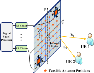
Figure 1: The MA-enabled multicast communication system

II System Model

II-A System Description

We consider a multicast communication system as depicted in Figure 1, where a transmitter with $N$ MAs sends the public message to two single-antenna user equipments (UEs). The transmit MAs are connected to RF chains via flexible cables, and thus their positions can be adjusted within a given two-dimensional region ${\mathcal{C}}$. Since practical electromechanical devices can only provide a horizontal or vertical movement by a fixed increment $d$ in each step [2, 3], the transmitter area of the MA-enabled communication system is quantized [3]. We collect the $M$ candidate discrete positions of the MAs in set ${\mathcal{P}}=\{{\mathbf{p}}_{m}=[\tilde{x}_{m},\tilde{y}_{m}]^{\mathsf{T}}\}_{m=1}^{M}$, where the distance between the neighboring positions is equal to $d$ in horizontal or vertical direction, as shown in Figure 1. The positions of the $n$th transmit MA can be represented by Cartesian coordinates ${\mathbf{t}}_{n}=[x_{n},y_{n}]^{\mathsf{T}}$. The above arguments imply that the feasible set of the $n$th transmit MA is given by $\mathcal{P}$, i.e., ${\mathbf{t}}_{n}\in{\mathcal{P}}$.

We assume quasi-static block-fading channels, and focus on one particular fading block with the multi-path channel components at any location in $\mathcal{C}$ given as fixed. For MA-enabled multicast communications, the channel is reconfigurable by adjusting the positions of MAs. Denote the collections of the coordinates of $N$ MAs by ${\mathcal{T}}=\{{\mathbf{t}}_{1}\ldots{\mathbf{t}}_{N}\}$. Then, the transmitter-to-UE $i$ channel vectors are given by ${\mathbf{h}}_{i}({\mathcal{T}})\in{\mathbbmss{C}}^{N\times 1}$ for $i\in\{1,2\}$, which are functions of ${\mathcal{T}}$. The transmitter can estimate the channel state information (CSI) of each UE by means of existing methods [8].

It is worth noting that the MA-based channel vectors are determined by the signal propagation environment and the positions of MAs. We consider the field-response based channel model given by ${\mathbf{h}}_{{i}}({\mathcal{T}})=[h_{i}({\mathbf{t}}_{1})\ldots h_{i}({\mathbf{t}}_{N})]^{\mathsf{T}}$, where [8]

$$h_{i}(\mathbf{x})\triangleq\sum_{l=1}^{L_{i}}\sigma_{l,i}{\rm{e}}^{{\rm{j}}\frac{2\pi}{\lambda}{\mathbf{x}}^{\mathsf{T}}{\bm{\rho}}_{l,i}},~{}i\in\{1,2\},$$ (1)

and where ${\bm{\rho}}_{l,i}=[\sin{\theta_{l,i}}\cos{\phi_{l,i}},\cos{\theta_{l,i}}]^{\mathsf{T}}$, $L_{i}$ is the number of resolvable paths, $\theta_{l,i}\in[0,\pi]$ and $\phi_{l,i}\in[0,\pi]$ are the elevation and azimuth angles of the $l$th path, respectively, $\sigma_{l,i}$ is the associated complex gain, and $\lambda$ is the wavelength.

The transmitter employs the linear beamformer ${\mathbf{w}}\in{\mathbbmss{C}}^{N\times 1}$ to construct the public multicast signal ${\mathbf{s}}\in{\mathbbmss{C}}^{N\times 1}$ from the data symbol $x\in{\mathbbmss{C}}$ which is considered to have zero mean and unit variance. The received signals at the UEs are thus given by ${y}_{i}={\mathbf{h}}_{i}^{\mathsf{H}}(\mathcal{T}){\mathbf{s}}+n_{i}={\mathbf{h}}_{i}^{\mathsf{H}}(\mathcal{T}){\mathbf{w}}x+n_{i}$ for $i\in\{1,2\}$, where $n_{i}\sim{\mathcal{CN}}(0,\sigma_{i}^{2})$ is the thermal noise at UE $i$ with $\sigma_{i}^{2}$ being the noise power. As a result, the multicast rate can be expressed as follows [10, 11]:

$${\mathcal{R}}=\log_{2}(1\!+\!\min\{\sigma_{1}^{-2}\lvert{\mathbf{h}}_{1}^{\mathsf{H}}(\mathcal{T}){\mathbf{w}}\rvert^{2},\sigma_{2}^{-2}\lvert{\mathbf{h}}_{2}^{\mathsf{H}}(\mathcal{T}){\mathbf{w}}\rvert^{2}\}).$$ (2)

Note that different from the conventional multicast channel with FPAs, the multicast rate for the MA-enabled multicast channel shown in (2) depends on the positions of MAs $\mathcal{T}$, which influence the channel vectors as well as the corresponding optimal beamformer.

II-B Problem Formulation

To reveal the fundamental rate limit of the MA-enabled multicast communication system, we assume that perfect CSI is available at both the transmitter and receiver. Then, we aim to maximize the multicast rate by jointly optimizing the MA positions $\mathcal{T}$ and the beamforming vector $\mathbf{w}$, subject to the discrete constraints on the MA positions and a power constraint at the transmitter. The optimization problem is thus given by

$$\max\nolimits_{\mathcal{T},{\mathbf{w}}}{\mathcal{R}}~{}{\rm{s.t.}}~{}\lVert\mathbf{w}\rVert^{2}\leq p,{\mathbf{t}}_{n}\in{\mathcal{P}},{\mathbf{t}}_{n}\neq{\mathbf{t}}_{n^{\prime}},n\neq n^{\prime}, {\mathcal{P}}_{1}$$ ()

where $p$ is the power budget. Note that (${\mathcal{P}}_{1}$) is a non-convex optimization problem due to the non-convexity of $\mathcal{R}$ with respect to $({\mathcal{T}},{\mathbf{w}})$ and the non-convex discrete position constraints ${\mathbf{t}}_{n}\in{\mathcal{P}}$. Moreover, the beamformer $\mathbf{w}$ is coupled with $\mathcal{T}$, which makes (${\mathcal{P}}_{1}$) challenging to solve.

III Proposed Solution

III-A General Case

III-A1 Transmit Beamforming Optimization

Due to the tight coupling of $\{\mathbf{w},\mathcal{T}\}$, we first derive the optimal beamforming vector for a given antenna position set $\mathcal{T}$. The subproblem of optimizing $\mathbf{w}$ is given by

$${\mathbf{w}}^{\star}=\operatorname*{argmax}\nolimits_{\lVert\mathbf{w}\rVert^{2}\leq p}\min\{\lvert\sigma_{1}^{-1}{\mathbf{h}}_{1}^{\mathsf{H}}(\mathcal{T}){\mathbf{w}}\rvert,\lvert\sigma_{2}^{-1}{\mathbf{h}}_{2}^{\mathsf{H}}(\mathcal{T}){\mathbf{w}}\rvert\}.$$

Based on the monotonicity of $\lvert{\mathbf{h}}_{1}^{\mathsf{H}}(\mathcal{T}){\mathbf{w}}\rvert^{2}$ and $\lvert{\mathbf{h}}_{2}^{\mathsf{H}}(\mathcal{T}){\mathbf{w}}\rvert^{2}$ with respect to $\lVert\mathbf{w}\rVert^{2}$, it is easily proved that $\lVert\mathbf{w}^{\star}\rVert^{2}=p$. Hence, we reformulate the above problem as follows:

$$\min\nolimits_{{\mathbf{p}},x}~{} f({\mathbf{p}},x)=-x$$ (3a)

$${\rm{s.t.}}~{} b_{i}({\mathbf{p}},x)=x-{\mathbf{p}}^{\mathsf{H}}\hat{\mathbf{h}}_{i}\hat{\mathbf{h}}_{i}^{\mathsf{H}}{\mathbf{p}}\leq 0,i=1,2$$ (3b)

$$h({\mathbf{p}},x)=\lVert\mathbf{p}\rVert^{2}-1,$$ (3c)

where $\hat{\mathbf{h}}_{i}=\frac{\sqrt{p}}{\sigma_{i}}\mathbf{h}_{i}(\mathcal{T})$ for $i=1,2$. Let $({\mathbf{p}}^{\star},x^{\star})$ denote the optimal solution of problem (3). Then, we have ${\mathbf{w}}^{\star}=\sqrt{p}{\mathbf{p}}^{\star}$, and the maximum multicast rate is given by $\log_{2}(1+x^{\star})$.

The optimal solution to problem (3) can be obtained from the Karush-Kuhn-Tucker (KKT) condition as follows [12]:

$$\nabla(-x)+\lambda\nabla(\lVert{\mathbf{p}}\rVert^{2}\!-\!1)+\mu_{1}\nabla b_{1}+\mu_{2}\nabla b_{2}={\mathbf{0}},$$ (4)

$$\mu_{1}b_{1}=0,\mu_{2}b_{2}=0,\lambda\in{\mathbbmss{R}},\mu_{1}\geq 0,\mu_{2}\geq 0,$$ (5)

where $\{\lambda,\mu_{1},\mu_{2}\}$ are real-valued Lagrangian multipliers. From (4), it can be shown that

$$(\mu_{1}\hat{\mathbf{h}}_{1}\hat{\mathbf{h}}_{1}^{\mathsf{H}}+\mu_{2}\hat{\mathbf{h}}_{2}\hat{\mathbf{h}}_{2}^{\mathsf{H}}){\mathbf{p}}=\lambda{\mathbf{p}},$$ (6)

$$\mu_{1}+\mu_{2}=1.$$ (7)

It is clear that the optimal beamformer ${\mathbf{p}}$ is an eigenvector of the matrix $(\sum_{i=1}^{2}\mu_{i}\hat{\mathbf{h}}_{i}\hat{\mathbf{h}}_{i}^{\mathsf{H}})$ with a corresponding eigenvalue $\lambda$. It follows from (7) that $\mu_{1}$ and $\mu_{2}$ cannot be $0$ at the same time. Moreover, from (6), we have

$$\mu_{1}{\mathbf{p}}^{\mathsf{H}}\hat{\mathbf{h}}_{1}\hat{\mathbf{h}}_{1}^{\mathsf{H}}{\mathbf{p}}+\mu_{2}{\mathbf{p}}^{\mathsf{H}}\hat{\mathbf{h}}_{2}\hat{\mathbf{h}}_{2}^{\mathsf{H}}{\mathbf{p}}=\lambda{\mathbf{p}}^{\mathsf{H}}{\mathbf{p}}=\lambda.$$ (8)

The above results suggest that $\lambda>0$. It is widely known that the eigenvector of $(\sum_{i=1}^{2}\mu_{i}\hat{\mathbf{h}}_{i}\hat{\mathbf{h}}_{i}^{\mathsf{H}})$ corresponding a non-zero eigenvalue can be written as the linear combination of $\hat{\mathbf{h}}_{1}$ and $\hat{\mathbf{h}}_{2}$. Therefore, we set ${\mathbf{p}}=a\hat{\mathbf{h}}_{1}+b\hat{\mathbf{h}}_{2}$. Particularly, we have ${\mathbf{p}}={\hat{\mathbf{h}}_{1}}/{\lVert\hat{\mathbf{h}}_{1}\rVert}$ for $\mu_{2}=0$ and $\mu_{1}>0$, and ${\mathbf{p}}={\hat{\mathbf{h}}_{2}}/{\lVert\hat{\mathbf{h}}_{2}\rVert}$ for $\mu_{1}=0$ and $\mu_{2}>0$. We then consider the case of $\mu_{1}>0$ and $\mu_{2}>0$, and it follows that

$$b_{i}=0\Leftrightarrow x={\mathbf{p}}^{\mathsf{H}}\hat{\mathbf{h}}_{i}\hat{\mathbf{h}}_{i}^{\mathsf{H}}{\mathbf{p}},~{}i=1,2.$$ (9)

Substituting ${\mathbf{p}}=a\hat{\mathbf{h}}_{1}+b\hat{\mathbf{h}}_{2}$ into (6) and (9) and performing some simple mathmematical manipulations, we have

$$a/b={{\mu_{1}}}/{(\mu_{2}{\rm{e}}^{-{\rm{j}}\angle\alpha_{12}})},$$ (10)

$$\mu_{1}(\alpha_{1}+\alpha_{12}b/a)=\mu_{2}(\alpha_{12}^{*}a/b+\alpha_{2})=\lambda,$$ (11)

where $\alpha_{1}=\lVert\hat{\mathbf{h}}_{1}\rVert^{2}$, $\alpha_{2}=\lVert\hat{\mathbf{h}}_{2}\rVert^{2}$, and $\alpha_{12}=\hat{\mathbf{h}}_{1}^{\mathsf{H}}\hat{\mathbf{h}}_{2}$.

By combining (7), (10), and (11), we have

$$\mu_{1}=\frac{\alpha_{2}-\lvert\alpha_{12}\rvert}{\alpha_{1}+\alpha_{2}-2\lvert\alpha_{12}\rvert},~{}\mu_{2}=\frac{\alpha_{1}-\lvert\alpha_{12}\rvert}{\alpha_{1}+\alpha_{2}-2\lvert\alpha_{12}\rvert},$$ (12)

which yields $\lambda=(\alpha_{1}\alpha_{2}-\lvert\alpha_{12}\rvert^{2})(\alpha_{1}+\alpha_{2}-2\lvert\alpha_{12}\rvert)^{-1}$ and

$${\mathbf{p}}=\frac{\mu_{1}\hat{\mathbf{h}}_{1}+\mu_{2}{\rm{e}}^{-{\rm{j}}\angle\alpha_{12}}\hat{\mathbf{h}}_{2}}{\sqrt{\mu_{1}^{2}\alpha_{1}+\mu_{2}^{2}\alpha_{2}+2\mu_{1}\mu_{2}\lvert\alpha_{12}\rvert}}.$$ (13)

It is worth noting that $\lambda=\mu_{1}^{2}\alpha_{1}+\mu_{2}^{2}\alpha_{2}+2\mu_{1}\mu_{2}\lvert\alpha_{12}\rvert$, and it follows that ${\mathbf{p}}={\mu_{1}}/{\sqrt{\lambda}}\hat{\mathbf{h}}_{1}+{\mu_{2}}/{\sqrt{\lambda}}{\rm{e}}^{-{\rm{j}}\angle\alpha_{12}}\hat{\mathbf{h}}_{2}$. Taken together, the optimal beamforming vector for a given position set $\mathcal{T}$ is given as follows:

$${\mathbf{w}}^{\star}=\left\{\begin{array}[]{ll}\sqrt{p}{{\mathbf{h}}_{1}(\mathcal{T})}/{\lVert{\mathbf{h}}_{1}(\mathcal{T})\rVert}&{\alpha_{1}\leq\lvert\alpha_{12}\rvert}\\ \sqrt{p}{{\mathbf{h}}_{2}(\mathcal{T})}/{\lVert{\mathbf{h}}_{2}(\mathcal{T})\rVert}&{\alpha_{2}\leq\lvert\alpha_{12}\rvert}\\ \frac{\sqrt{p}\mu_{1}{\mathbf{h}}_{1}(\mathcal{T})}{\sigma_{1}\sqrt{\lambda}\lVert{\mathbf{h}}_{1}(\mathcal{T})\rVert}+\frac{\sqrt{p}\mu_{2}{\mathbf{h}}_{2}(\mathcal{T}){\rm{e}}^{-{\rm{j}}\angle\alpha_{12}}}{\sigma_{2}\sqrt{\lambda}\lVert{\mathbf{h}}_{2}(\mathcal{T})\rVert}&{\text{else}}\end{array}\right..$$ (14)

III-A2 Antenna Position Optimization

The above arguments imply that given the antenna position set $\mathcal{T}$, the maximum multicast rate satisfies

$${\mathcal{R}}_{1}(\mathcal{T})=\left\{\begin{array}[]{ll}\log_{2}(1\!+\!\alpha_{1})&{\alpha_{1}\leq\lvert\alpha_{12}\rvert}\\ \log_{2}(1\!+\!\alpha_{2})&{\alpha_{2}\leq\lvert\alpha_{12}\rvert}\\ \log_{2}(1\!+\!\frac{\alpha_{1}\alpha_{2}-\lvert\alpha_{12}\rvert^{2}}{\alpha_{1}+\alpha_{2}-2\lvert\alpha_{12}\rvert})&{\text{else}}\end{array}\right.\!\!\!,$$ (15)

which features a function of $\mathcal{T}$. Based on this, we can equivalently transform problem (${\mathcal{P}}_{1}$) as follows:

$$\max\nolimits_{\mathcal{T}}{\mathcal{R}}_{1}(\mathcal{T})~{}~{}{\rm{s.t.}}~{}{\mathbf{t}}_{n}\in{\mathcal{P}},{\mathbf{t}}_{n}\neq{\mathbf{t}}_{n^{\prime}},n\neq n^{\prime}.$$ (16)

Despite involving more tractability than problem (${\mathcal{P}}_{1}$), problem (16) is yet a non-convex inter programming. Problem (16) is NP-hard, and applying the exhaustive search to finding its optimal solution is computationally costly. To handle this difficulty, we propose a greedy search-based algorithm to approximate the optimal design with reduced complexity.

The greedy search comprises $N$ step, where at the $n$th step, the candidate antenna position with index $J_{n}$ is selected from the candidate set $\mathcal{J}$ to maximize the increment of the objective function ${\mathcal{R}}_{1}(\cdot)$ [14]. On this basis, we can obtain

$$J_{n}=\operatorname*{argmax}\nolimits_{j\in{\mathcal{J}}}({\mathcal{R}}_{1}({\mathcal{S}}_{n-1}\cup\{{\mathbf{p}}_{j}\})-{\mathcal{R}}_{1}({\mathcal{S}}_{n-1})),$$ (17)

where the set ${\mathcal{S}}_{n-1}$ stores the Cartesian coordinates of the selected candidate antenna positions after $n-1$ steps. Taking the above steps together, we conclude a greedy search-based algorithm that is represented in Algorithm 1.

Algorithm 1 The proposed greedy search-based method for solving problem (${\mathcal{P}}_{1}$)

1:  ${\mathcal{J}}=\{1,\ldots,M\}$, $n=0$, ${\mathcal{S}}_{n}=\emptyset$

2:  repeat

3:     Set $n=n+1$ and update $J_{n}$ based on (17)

4:     Update ${\mathcal{S}}_{n}$ as ${\mathcal{S}}_{n-1}\cup J_{n}$

5:  until $n=N$

6:  Set the MA position set as ${\mathcal{T}}=\{{\mathbf{p}}_{i}\}_{i\in{\mathcal{S}}_{N}}$

7:  Design the bamforming vector $\mathbf{w}$ by (14) for the given MA positions ${\mathcal{T}}$

We note that ${\mathcal{R}}_{1}(\cdot)$ shown in (15) is a piecewise function. Regarding the practical implementation of Algorithm 1, one could set the objective function ${\mathcal{R}}_{1}(\cdot)$ as $\log_{2}(1+\alpha_{i})$ and $\log_{2}(1+\frac{\alpha_{1}\alpha_{2}-\lvert\alpha_{12}\rvert^{2}}{\alpha_{1}+\alpha_{2}-2\lvert\alpha_{12}\rvert})$, respectively, and return the feasible solution of $\mathcal{T}$ that achieves the maximum objective value.

III-B Special Case: LOS Transmission

We consider LOS propagation as a special case of problem (${\mathcal{P}}_{1}$), where $L_{1}=L_{2}=1$. Besides, we assume that the two UEs suffer from the same path loss, i.e., $\lvert\sigma_{1,1}\rvert^{2}=\lvert\sigma_{1,2}\rvert^{2}=\kappa$, which can happen when the two UEs are equidistant from the transmitter. For brevity, it is further assumed that $\sigma_{1}^{2}=\sigma_{2}^{2}=\sigma^{2}$. Under the above assumptions, we simplify (15) as

$${\mathcal{R}}_{1}(\mathcal{T})\!=\!\left\{\begin{array}[]{ll}\!\!\!\log_{2}(1\!+\!\frac{pN\kappa}{\sigma^{2}})&{\alpha_{1}~{}{\text{or}}~{}\alpha_{2}\!\leq\!\lvert\alpha_{12}\rvert}\\ \!\!\!\log_{2}(1\!+\!\frac{p\kappa(N+\lvert{\mathbf{a}}_{1}^{\mathsf{H}}(\mathcal{T}){\mathbf{a}}_{2}(\mathcal{T})\rvert)}{2\sigma^{2}})&{\text{else}}\end{array}\right.\!\!\!,$$

where ${\mathbf{a}}_{i}(\mathcal{T})=[{\rm{e}}^{{\rm{j}}\frac{2\pi}{\lambda}{\mathbf{t}}_{1}^{\mathsf{T}}{\bm{\rho}}_{1,i}}\ldots{\rm{e}}^{{\rm{j}}\frac{2\pi}{\lambda}{\mathbf{t}}_{N}^{\mathsf{T}}{\bm{\rho}}_{1,i}}]^{\mathsf{T}}$ for $i\in\{1,2\}$.

Let ${\mathbf{a}}=[a_{1},\ldots,a_{M}]^{\mathsf{T}}\in\{0,1\}^{M\times 1}$ denote the MA position determination vector, with $a_{m}=1$ and $a_{m}=0$ representing that an MA is placed and not placed on the position ${\mathbf{p}}_{m}$, respectively. Then, we obtain ${\mathcal{T}}=\{{\mathbf{p}}_{m}|a_{m}=1\}$ and

$$\lvert{\mathbf{a}}_{1}^{\mathsf{H}}(\mathcal{T}){\mathbf{a}}_{2}(\mathcal{T})\rvert^{2}={{\mathbf{a}}^{\mathsf{T}}{\mathbf{Q}}{\mathbf{a}}},$$ (18)

where ${\mathbf{Q}}=\Re\{{\mathbf{g}}\}\Re\{{\mathbf{g}}^{\mathsf{T}}\}+\Im\{{\mathbf{g}}\}\Im\{{\mathbf{g}}^{\mathsf{T}}\}$, ${\mathbf{g}}={\mathbf{g}}_{1}^{*}\odot{\mathbf{g}}_{2}$, and ${\mathbf{g}}_{i}=[{\rm{e}}^{{\rm{j}}\frac{2\pi}{\lambda}{\mathbf{p}}_{1}^{\mathsf{T}}{\bm{\rho}}_{1,i}}\ldots{\rm{e}}^{{\rm{j}}\frac{2\pi}{\lambda}{\mathbf{p}}_{M}^{\mathsf{T}}{\bm{\rho}}_{1,i}}]^{\mathsf{T}}$ for $i=1,2$. Taken together, problem (16) is simplified as follows:

$${\mathbf{a}}^{\star}=\operatorname*{argmax}\nolimits_{a_{m}\in\{0,1\},\sum_{m=1}^{M}a_{m}=N}{{\mathbf{a}}^{\mathsf{T}}{\mathbf{Q}}{\mathbf{a}}}.$$ (19)

We next propose a BAB-based method to find ${\mathbf{a}}^{\star}$ with reduced complexity compared with the exhaustive search.

Let $\mathcal{S}$ and $\mathcal{J}$ store the indices of the determined MA positions and candidate MA positions. Initially, $\mathcal{S}$ is set as an empty set and ${\mathcal{J}}={\mathcal{J}}_{0}\triangleq\{1,\ldots,M\}$. Moreover, let ${\mathbf{a}}_{n}$ and $f_{n}$ denote the position determination vector and the associated objective function value for the determined $n$ ($n\leq N$) MA positions, i.e., $f_{n}={{\mathbf{a}}_{n}^{\mathsf{T}}{\mathbf{Q}}{\mathbf{a}}}_{n}$. Suppose that $J_{n+1}$ is the index of the $(n+1)$th determined position. Then, we update $\mathcal{S}$ and $\mathcal{J}$ as ${\mathcal{S}}={\mathcal{S}}\cup\{J_{n+1}\}$ and ${\mathcal{J}}={\mathcal{J}}\setminus\{J_{n+1}\}$, respectively. Besides, $f_{n+1}$ can be recursively computed by

$$f_{n+1}=f_{n}+2[{{\mathbf{Q}}{\mathbf{a}}_{n}^{\mathsf{T}}}]_{J_{n+1}}+[{\mathbf{Q}}]_{J_{n+1},J_{n+1}},$$ (20)

where $f_{0}=0$, ${\mathbf{a}}_{0}={\mathbf{0}}$, and $[\mathbf{x}]_{i}$ and $[\mathbf{X}]_{i,j}$ extract the $i$th and $(i,j)$th elements of vector $\mathbf{x}$ and matrix $\mathbf{X}$, respectively. As suggested in [15], the BAB-based method is more efficient for maximizing a monotonic decreasing objective function or minimizing a monotonic increasing objective function. To this end, we modify the original objective $f_{n}$ as follows:

$$\overline{f}_{n}=f_{n}-2n{\mathsf{X}}-n{\mathsf{Y}},$$ (21)

where ${\mathsf{X}}=\max\nolimits_{j\in{\mathcal{J}}_{0}}[{\ddot{\mathbf{Q}}{\mathbf{1}}^{\mathsf{T}}}]_{j}$, ${\mathsf{Y}}=\max\nolimits_{j\in{\mathcal{J}}_{0}}[{\mathbf{Q}}]_{j,j}$, and the operator $\ddot{\mathbf{X}}$ takes the element-wise absolute value of matrix ${\mathbf{X}}$. Therefore, $\overline{f}_{n}$ can be recursively updated by

$$\overline{f}_{n+1}=\overline{f}_{n}\!+\!2[{{\mathbf{Q}}{\mathbf{a}}_{n}^{\mathsf{T}}}]_{J_{n+1}}\!-\!2{\mathsf{X}}\!+\![{\mathbf{Q}}]_{J_{n+1},J_{n+1}}\!-\!{\mathsf{Y}}.$$ (22)

It is readily shown that $[{{\mathbf{Q}}{\mathbf{a}}_{n}^{\mathsf{T}}}]_{J_{n+1}}<{\mathsf{X}}$ and $[{\mathbf{Q}}]_{J_{n+1},J_{n+1}}\leq{\mathsf{Y}}$, which yields $\overline{f}_{n+1}<\overline{f}_{n}$. This means that $\overline{f}_{n}$ is monotonically decreasing with respect to the subset size. Note that the objective function value in the last step, i.e., $\overline{f}_{N}$, equals ${f}_{N}$ plus a fixed offset $2L{\mathsf{X}}+N{\mathsf{Y}}$ that only depends on $\mathbf{Q}$, and is irrelevant to $\mathbf{a}$. Taken together, we can get

$${\mathbf{a}}^{\star}=\operatorname*{argmax}\nolimits_{\mathbf{a}}{f_{N}}=\operatorname*{argmax}\nolimits_{\mathbf{a}}{\overline{f}_{N}}.$$ (23)

Figure 2: An example of search tree with $M=6$ and $N=2$

The BAB-based method is best understood by treating the whole procedure of position determination as a tree search. Figure 2 shows an example of search tree when $M=6$ and $N=2$, where the number on each node denotes the position index. In each tree level, an position node is selected until the leaf nodes. A path from the root to a leaf node corresponds to one candidate subset of position indices. The search procedure aims to find the path that maximizes $\overline{f}_{N}$ in the tree.

We initialize a global lower bound $B=-\infty$ and exploit a best-first strategy. The search procedure will start from the root node and go further to the higher levels. For the currently visited node at level $n$, we evaluate the corresponding objective $\overline{f}_{n}$. If $\overline{f}_{n}<B$, due to the decreasing monotonicity of the objective function, all its child nodes yield lower values of $\overline{f}_{n+1}$ than $B$, which means that all these child nodes will not be necessarily evaluated and will hence be pruned; otherwise, the child nodes will be explored from the best one which has the least $\overline{f}_{n+1}$ to the largest one. When a leaf node is visited, we need to update the global bound as $B=\overline{f}_{N}$ if $\overline{f}_{N}>B$. When all the subtree nodes of the currently visited node are evaluated or pruned, the search will go back to its parent nodes to evaluate other subtrees. The above procedure will be repeated until all the nodes are evaluated or pruned, thus giving a globally optimal solution. In contrast to the exhaustive search, the BAB-based search results in reduced computational complexity thanks to the pruning operation.

Algorithm 2 The BAB-based method for solving (19)

1:  $B=-\infty$, $n=0$, $\overline{{f}}_{{{n}}}=0$, ${\mathbf{u}}={\mathbf{0}}$, $K=0$

2:  if $n=L-1$ then

3:     ${c_{k}}=\overline{{f}}_{{{n}}}+2[{{\mathbf{Q}}{\mathbf{u}}^{\mathsf{T}}}]_{k}-2{\mathcal{X}}+[{\mathbf{Q}}]_{k,k}-{\mathcal{Y}},\forall{k}\in{\mathcal{I}}_{n,{K}}$

4:     if $\max_{{k}\in{\mathcal{I}}_{n,{K}}}{c_{k}}>B$ then

5:        Set $[{\mathbf{u}}]_{\operatorname*{argmax}_{{k}\in{\mathcal{I}}_{n,{K}}}{c_{k}}}=1$

6:        Update the global lower bound $B=\max_{{k}\in{\mathcal{I}}_{n,{K}}}{c_{k}}$

7:     end if

8:  else

9:     ${c_{k}}=\overline{{f}}_{{{n}}}+2[{{\mathbf{Q}}{\mathbf{u}}^{\mathsf{T}}}]_{k}-2{\mathcal{X}}+[{\mathbf{Q}}]_{k,k}-{\mathcal{Y}},\forall{k}\in{\mathcal{I}}_{n,{K}}$

10:     Sort ${c_{k}},\forall{k}\in{\mathcal{I}}_{n,{K}}$ in a descending order to get an ordered index vector ${\mathbf{k}}$

11:     for $i=1:\left|{\mathcal{I}}_{n,{K}}\right|$ do

12:        if $c_{[{\mathbf{k}}]_{i}}>B$ then

13:           Set $[{\mathbf{v}}]_{[{\mathbf{k}}]_{i}}=1$, $\overline{{f}}_{{{n+1}}}=c_{[{\mathbf{k}}]_{i}}$, and $K=[{\mathbf{k}}]_{i}$

14:           Set $n={n+1}$, and go to line 2

15:        else

16:           Break the loop

17:        end if

18:     end for

19:  end if

20:  Set the position determination vector as ${\mathbf{a}}={\mathbf{u}}$

21:  Design the bamforming vector $\mathbf{w}$ by (14) for the given MA positions ${\mathcal{T}}$

As a consequence of the above arguments, the proposed BAB-based method for solving problem (19) is summarized in Algorithm 2, where ${\mathcal{I}}_{l,{K}}$ is the child node index set of node $K$ in level $l$ with ${\mathcal{I}}_{0,{0}}=\{1,\ldots,M-N+1\}$. It is shown that the computational complexity of Algorithm 2 scales with ${\mathcal{O}}(N_{\rm{v}}N)$, where $N_{\rm{v}}$ represents the number of visited nodes during the tree search.

IV Numerical Results

In this section, numerical results are provided to validate the effectiveness of our proposed algorithms. In the simulation, we consider a transmitter with $N=4$ MAs. The transmit area is quantized into a discrete square grid of size $\sqrt{M}\times\sqrt{M}$ with equal distance $d=\frac{\lambda}{2}$, as shown in Figure 1. We consider the LOS channel model, where $L_{1}=L_{2}=1$, $\lvert\sigma_{1,1}\rvert^{2}=\lvert\sigma_{1,2}\rvert^{2}=1$, and the elevation and azimuth angles are randomly set within $[0,\pi]$. The following numerical results are averaged over 1000 independent channel realizations.

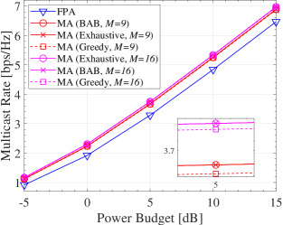
Figure 3: Multicast rate vs. the power budget.

Next, we compare the performance of our proposed algorithms with the FPA-based benchmark scheme, where the transmitter is equipped with FPA-based uniform linear array with $N$ antennas spaced by $\frac{\lambda}{2}$.

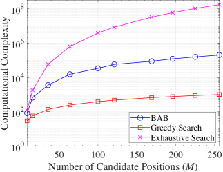
Figure 4: Computational complexity vs. the number of candidate positions.

In Figure 3, we show the multicast rate of the proposed and benchmark schemes versus the transmit power $p$. It is observed that with the same power, our proposed algorithm can achieve a larger multicast rate as compared to the FPA-based scheme. Besides, the rate gap increases with the number of candidate discrete positions, $M$. We also observe that the BAB-based method achieves a multicast rate equivalent to the exhaustive search, while the greedy search exhibits virtually the same rate performance to the BAB-based method. Figure 4 illustrates the computational complexity, i.e., the number of visited nodes in the search tree, versus $M$. We can see that the BAB search has a complexity in-between the greedy search and exhaustive search. The above results suggest that the greedy search strikes an effective performance/complexity trade-off, rendering it a compelling candidate for practical MA-enabled communication systems.

V Conclusion

In this paper, we investigated the joint optimization of transmit beamformer and transmit MA positions to maximize the transmission rate for a two-user MA-enabled MISO communication system. Due to the practical hardware limits, we modeled the movement of the MA elements as a discrete motion. We proposed an efficient greedy search-based algorithm to handle the formulated problem. We showed that when the two users experience comparable LOS path losses, the globally optimal solution to this problem can be attained through a BAB search. Numerical results revealed the superiority of the proposed MA-enabled multicast system. In future work, we will develop a computationally efficient scheme tailored to practical MA-enabled systems with a larger number of UEs.

References

• [1] L. Zhu et al., “Modeling and performance analysis for movable antenna enabled wireless communications,” IEEE Trans. Wireless Commun., Early Access, 2023.
• [2] T. Ismail and M. Dawoud, “Null steering in phased arrays by controlling the elements positions,” IEEE Trans. Antennas Propagat., vol. 39, no. 11, pp. 1561–1566, Nov. 1991.
• [3] S. Basbug, “Design and synthesis of antenna array with movable elements along semicircular paths,” IEEE Antennas Wireless Propag. Lett., vol. 16, pp. 3059–3062, Oct. 2017.
• [4] L. Zhu et al., “Movable antennas for wireless communication: Opportunities and challenges,” IEEE Commun. Mag., Early Access, 2023.
• [5] W. Ma, L. Zhu, and R. Zhang, “MIMO capacity characterization for movable antenna systems,” IEEE Trans. Wireless Commun., Early Access, 2023.
• [6] L. Zhu et al., “Movable-antenna enhanced multiuser communication via antenna position optimization,” IEEE Trans. Wireless Commun., Early Access, 2023.
• [7] Y. Wu et al., “Movable antenna-enhanced multiuser communication: Optimal discrete antenna positioning and beamforming,” arXiv:2308.02304, 2023.
• [8] W. Ma et al., “Compressed sensing based channel estimation for movable antenna communications,” IEEE Commun. Lett., vol. 27, no. 10, Oct. 2023.
• [9] N. Golrezaei, A. F. Molisch, A. G. Dimakis, and G. Caire, “Femtocaching and device-to-device collaboration: A new architecture for wireless video distribution,” IEEE Commun. Mag., vol. 51, no. 4, pp. 142–149, Apr. 2013.
• [10] N. D. Sidiropoulos, T. N. Davidson, and Z. Luo, “Transmit beamforming for physical-layer multicasting,” IEEE Trans. Signal Process., vol. 54, no. 6, pp. 2239–2251, Jun. 2006.
• [11] N. Jindal and Z.-Q. Luo, “Capacity limits of multiple antenna multicast,” in Proc. IEEE Int. Symposium Inf. Theory (ISIT), pp. 1841–1845, 2006.
• [12] S. Boyd and L. Vandenberghe, Convex Optimization. Cambridge, U.K.: Cambridge Univ. Press, 2004.
• [13] R. A. Horn and C. R. Johnson, Matrix Analysis, 2nd ed. New York, NY, USA: Cambridge Univ. Press, 2012.
• [14] M. Gharavi-Alkhansari and A. B. Gershman, “Fast antenna subset selection in MIMO systems,” IEEE Trans. Signal Process., vol. 52, no. 2, pp. 339–347, Feb. 2004.
• [15] P. M. Narendra and K. Fukunaga, “A branch and bound algorithm for feature subset selection,” IEEE Trans. Comput., vol. C-26, no. 9, pp. 917–922, Sep. 1977.