Distribution-Preserving Integrated Sensing and Communication with Secure Reconstruction

Yiqi Chen1, Tobias Oechtering2, Holger Boche3, Mikael Skoglund2, and Yuan Luo1


Yiqi Chen and Yuan Luo were supported in part by National Key R&D Program of China under Grant 2022YFA1005000, and National Natural Science Foundation of China under Grant 62171279.Holger Boche was supported by the German Federal Ministry of Education and Research (BMBF) within the programme of โ€Souverรคn. Digital. Vernetztโ€, research HUB 6G-life, project identification number: 16KISK002, and by the BMBF Quantum Projects QuaPhySI, Grant 16KIS1598K, and QUIET, Grant 16KISQ093. 1Shanghai Jiao Tong University, Shanghai, China, {chenyiqi,yuanluo}@sjtu.edu.cn 2KTH Royal Institute of Technology, 100 44 Stockholm, Sweden, {oech,skoglund}@kth.se 3Technical University of Munich, 80290 Munich, Germany, boche@tum.de
Abstract

Distribution-preserving integrated sensing and communication with secure reconstruction is investigated in this paper. In addition to the distortion constraint, we impose another constraint on the distance between the reconstructed sequence distribution and the original state distribution to force the system to preserve the statistical property of the channel states. An inner bound of the distribution-preserving capacity-distortion region is provided with some capacity region results under special cases. A numerical example demonstrates the tradeoff between the communication rate, reconstruction distortion and distribution preservation. Furthermore, we consider the case that the reconstructed sequence should be kept secret from an eavesdropper who also observes the channel output. An inner bound of the tradeoff region and a capacity-achieving special case are presented.

I introduction

Integrated sensing and communication (ISAC) is regarded as a promising feature of future wireless communication techniques such as 6G[1]. It opens up completely new use cases and possibilities for users and operators for 6G, but it also poses special challenges for the design of communication systems. In particular, the misuse of ISAC could significantly increase the attack surface for security and privacy attacks on 6G [2][3]. However, security and privacy are essential prerequisites for a trustworthy 6G system [2][3]. Therefore, it is of fundamental importance to further develop the theoretical foundations of ISAC to prevent misuse of ISAC technology.

In [4], the author addressed the rate-distortion tradeoff for decoder side sensing, with the channel states known at the encoder side noncausally. Further developments can be found in [5] for state amplification and [6] where the states are not available at the encoder. In [7], the sender is interested in not only the information transmission, but also the estimation of the channel states for discrete channels. Fundamental limits of the capacity-distortion tradeoff for several channel models were provided. Extensions on ISAC over Gaussian channels were provided in [8]. The secure ISAC system was studied in [9], where the feedback signal is used for both sensing and secret key generation to protect the transmitted message. ISAC with binary input and additive white Gaussian noise was studied in [10]. Source coding with distribution-preservation can be found in [11, 12, 13]

Refer to caption
Figure 1: The state estimator has all the information at the encoder side with an additional feedback sequence $z^{n}$. It tries to reconstruct the state sequence preserving the distribution. The henchman shares all the information at the state estimator and communicates to the eavesdropper with a limited rate.

This paper considers a distribution-preserving ISAC system in that we not only reconstruct the state sequence within a given distortion constraint, but also require the distribution of the reconstructed sequence to be close to the original state distribution. This model is motivated by the fact that the ultimate goal of sensing is to learn the environment and design a better communication strategy for the system using the sensed state data. By preserving the state distribution, one can build a system for a specific environment and hence avoid the effect of the distribution mismatch problem. To better understand the impact of ISAC on the security and privacy attack surface for future communication systems such as 6G, we further introduce a Henchman and Eavesdropper model into the ISAC framework and investigate the corresponding rate-distortion region.

II model and results

Throughout this paper, random variable, sample value and its alphabet are denoted by capital, lowercase letters, and calligraphic letters, respectively, e.g. $X$, $x$, and $\mathcal{X}$. Symbols $X^{n}$ and $x^{n}$ represent random sequence and its sample value with length $n$. The distribution of a random variable $X$ is denoted by $P_{X}$ and the joint distribution of a pair of random variables $(X,Y)$ is denoted by $P_{XY}$. The expectation of a function of the random variable $X$ is written by $\mathbb{E}_{X}\left[f(X)\right]$. Consider a communication system where the sender receives a feedback sequence after sending a codeword to the receiver through a state-dependent channel and then estimates the channel state based on the knowledge it has. Furthermore, we assume the sender has a noisy observation of the channel state sequence in a noncausal manner, which represents some prior knowledge of the environment at the encoder side. Compared to the existing ISAC model[7] that has a distortion constraint on the reconstructed sequence, the state estimator here is imposed an additional distribution constraint. In more detail, we want the distribution of the reconstructed sequence to be close to the original sequence under a given distance metric.

From a more practical point of view, for any state-dependent system, which is governed by an i.i.d. generated state sequence $S^{n}$ and equipped with an ISAC system, the sensing result $\hat{S}^{n}$ is used for further processing, which is usually characterized by a bounded function $\kappa:\mathcal{S}^{n}\to\mathbb{R}$ such that maxs^nโก|ฮบโ€‹(s^n)|โ‰คฮฅsubscriptsuperscript^๐‘ ๐‘›๐œ…superscript^๐‘ ๐‘›ฮฅ\max_{\hat{s}^{n}}|\kappa(\hat{s}^{n})|\leq\Upsilon, where $\Upsilon$ is a positive number and $\mathcal{S}$ is the common alphabet of $S$ and $\hat{S}$. We denote the distributions of $S^{n}$ and $\hat{S}^{n}$ by $P^{n}_{S}=\prod_{i=1}^{n}P_{S}$ and $P_{\hat{S}^{n}}$ for a moment. The processing functions $\kappa$ vary depending on different objectives of the system with a consensus that the processing result of the estimated sequence should be close to that of the original sequence, regardless of what the function $\kappa$ is. We control this gap between the estimation and the original sequences by controlling

supฮบ:maxs^nโก|ฮบโ€‹(s^n)|โ‰คฮฅ|๐”ผPSnโ€‹[ฮบโ€‹(Sn)]โˆ’๐”ผPS^nโ€‹[ฮบโ€‹(S^n)]|,subscriptsupremum:๐œ…subscriptsuperscript^๐‘ ๐‘›๐œ…superscript^๐‘ ๐‘›ฮฅsubscript๐”ผsubscriptsuperscript๐‘ƒ๐‘›๐‘†delimited-[]๐œ…superscript๐‘†๐‘›subscript๐”ผsubscript๐‘ƒsuperscript^๐‘†๐‘›delimited-[]๐œ…superscript^๐‘†๐‘›\displaystyle\sup_{\kappa:\;\max_{\hat{s}^{n}}|\kappa(\hat{s}^{n})|\leq\Upsilon}\left|\mathbb{E}_{P^{n}_{S}}\left[\kappa(S^{n})\right]-\mathbb{E}_{P_{\hat{S}^{n}}}\left[\kappa(\hat{S}^{n})\right]\right|, (1)

which can be further bounded by
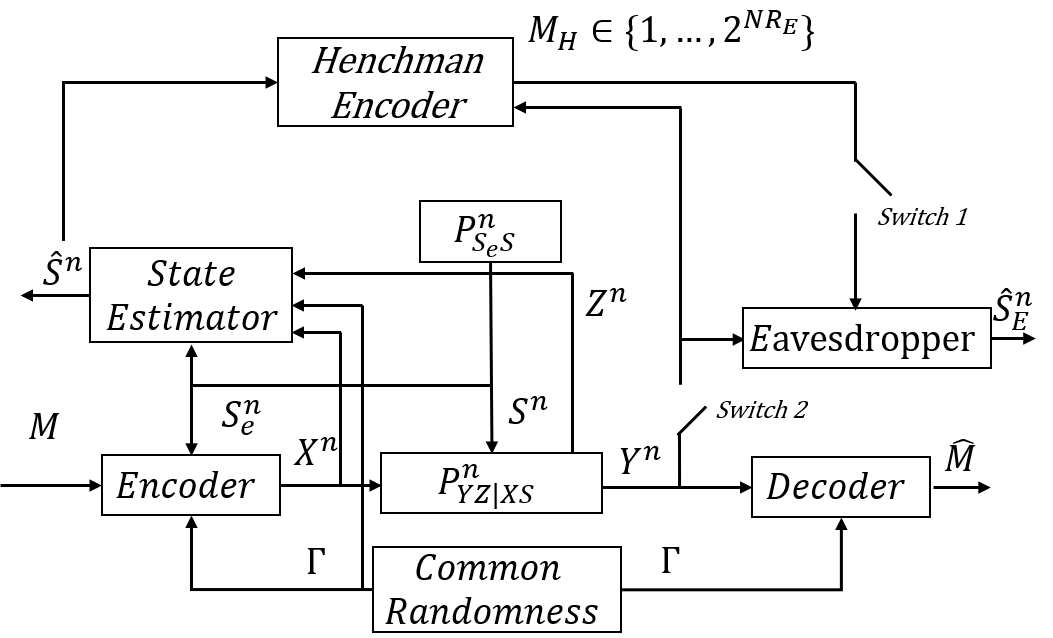
supฮบ:maxs^nโก|ฮบโ€‹(s^n)|โ‰คฮฅ|๐”ผPSnโ€‹[ฮบโ€‹(Sn)]โˆ’๐”ผPS^nโ€‹[ฮบโ€‹(S^n)]|subscriptsupremum:๐œ…subscriptsuperscript^๐‘ ๐‘›๐œ…superscript^๐‘ ๐‘›ฮฅsubscript๐”ผsubscriptsuperscript๐‘ƒ๐‘›๐‘†delimited-[]๐œ…superscript๐‘†๐‘›subscript๐”ผsubscript๐‘ƒsuperscript^๐‘†๐‘›delimited-[]๐œ…superscript^๐‘†๐‘›\displaystyle\sup_{\begin{subarray}{c}\kappa:\;\max_{\hat{s}^{n}}|\kappa(\hat{s}^{n})|\leq\Upsilon\end{subarray}}\left|\mathbb{E}_{P^{n}_{S}}\left[\kappa(S^{n})\right]-\mathbb{E}_{P_{\hat{S}^{n}}}\left[\kappa(\hat{S}^{n})\right]\right|
=(a)โ€‹maxฮบ:maxs^nโก|ฮบโ€‹(s^n)|โ‰คฮฅโก|๐”ผPSnโ€‹[ฮบโ€‹(Sn)]โˆ’๐”ผPS^nโ€‹[ฮบโ€‹(S^n)]|๐‘Žsubscript:๐œ…subscriptsuperscript^๐‘ ๐‘›๐œ…superscript^๐‘ ๐‘›ฮฅsubscript๐”ผsubscriptsuperscript๐‘ƒ๐‘›๐‘†delimited-[]๐œ…superscript๐‘†๐‘›subscript๐”ผsubscript๐‘ƒsuperscript^๐‘†๐‘›delimited-[]๐œ…superscript^๐‘†๐‘›\displaystyle\overset{(a)}{=}\max_{\begin{subarray}{c}\kappa:\;\max_{\hat{s}^{n}}|\kappa(\hat{s}^{n})|\leq\Upsilon\end{subarray}}\left|\mathbb{E}_{P^{n}_{S}}\left[\kappa(S^{n})\right]-\mathbb{E}_{P_{\hat{S}^{n}}}\left[\kappa(\hat{S}^{n})\right]\right|
โ‰คฮฅโ€‹โˆ‘snโˆˆ๐’ฎn|PSnโ€‹(sn)โˆ’PS^nโ€‹(sn)|absentฮฅsubscriptsuperscript๐‘ ๐‘›superscript๐’ฎ๐‘›subscriptsuperscript๐‘ƒ๐‘›๐‘†superscript๐‘ ๐‘›subscript๐‘ƒsuperscript^๐‘†๐‘›superscript๐‘ ๐‘›\displaystyle\leq\Upsilon\sum_{s^{n}\in\mathcal{S}^{n}}\left|P^{n}_{S}(s^{n})-P_{\hat{S}^{n}}(s^{n})\right|

where $(a)$ is by the fact that the set of functions $\kappa$ is a compact set. This implies that with a reconstructed distribution that is sufficiently close to the original one, we can control the expectation of the processing result defined in (1) no matter which processing function is used. We further consider the case where there exists a henchman in the state estimator and an eavesdropper who both observe the channel output. The henchman sends messages to the eavesdropper with a limited rate and the goal of the henchman is to reconstruct the state as well. The model is illustrated in Fig. 1. In the following, we consider the model without secure constraint, which is the case that Switches 1 and 2 are turned off. A code used for such a communication system is defined as follows.

Definition 1.

A common randomness (CR)-assisted code $(n,R,R_{c})$ for distribution preserving ISAC with noisy channel state information (NCSI) consists of

  • โ€ข

    A message set $\mathcal{M}=[1:2^{nR}]$,

  • โ€ข

    Common randomness available both at the encoder and decoder $\Gamma\in[1:2^{nR_{c}}]$,

  • โ€ข

    An encoder $f:\mathcal{M}\times\mathcal{S}^{n}_{e}\times\Gamma\to\mathcal{X}^{n}$,

  • โ€ข

    A decoder $g:\mathcal{Y}^{n}\times\Gamma\to\mathcal{M}$,

  • โ€ข

    A state estimator $h:\Gamma\times\mathcal{X}^{n}\times\mathcal{S}^{n}_{e}\times\mathcal{Z}^{n}\to\hat{\mathcal{S}}^{n}$.

Throughout this paper, we use total variation as the distance metric between two distributions, and denote it by $||P-Q||$ for distributions $P$ and $Q$ on the same alphabet.

Definition 2.

Given non-negative real numbers $(D,\Delta)$, a pair $(R,R_{c})$ is said to be $(D,\Delta)-$achievable if for any $\epsilon>0$ and sufficiently large $n$, there exists an $(n,R,R_{c})$ code such that

Pโ€‹rโ€‹{Mโ‰ M^}โ‰คฯต,๐”ผโ€‹[dโ€‹(Sn,S^n)]โ‰คD,โ€–PS^nโˆ’ฯˆnโ€–โ‰คฮ”,formulae-sequence๐‘ƒ๐‘Ÿ๐‘€^๐‘€italic-ฯตformulae-sequence๐”ผdelimited-[]๐‘‘superscript๐‘†๐‘›superscript^๐‘†๐‘›๐ทnormsubscript๐‘ƒsuperscript^๐‘†๐‘›superscript๐œ“๐‘›ฮ”\begin{split}Pr\{M\neq\hat{M}\}\leq\epsilon,\;\mathbb{E}\left[d(S^{n},\hat{S}^{n})\right]\leq D,||P_{\hat{S}^{n}}-\psi^{n}||\leq\Delta,\end{split} (2)

where $\psi$ is the distribution of the channel state.

Given state source distribution $P_{S_{e}S}$ with marginal distribution $P_{S}=\psi$ and channel $P_{YZ|XS}$, let $\mathcal{P}(U,X,\hat{S})$ be the set of joint distribution $P_{S_{e}SUXYZ\hat{S}}$ such that

PSeโ€‹Sโ€‹Uโ€‹Xโ€‹Yโ€‹Zโ€‹S^โ€‹(se,s,u,x,y,z,s^)=PSeโ€‹Sโ€‹(se,s)โ€‹PU|Seโ€‹(u|se)subscript๐‘ƒsubscript๐‘†๐‘’๐‘†๐‘ˆ๐‘‹๐‘Œ๐‘^๐‘†subscript๐‘ ๐‘’๐‘ ๐‘ข๐‘ฅ๐‘ฆ๐‘ง^๐‘ subscript๐‘ƒsubscript๐‘†๐‘’๐‘†subscript๐‘ ๐‘’๐‘ subscript๐‘ƒconditional๐‘ˆsubscript๐‘†๐‘’conditional๐‘ขsubscript๐‘ ๐‘’\displaystyle P_{S_{e}SUXYZ\hat{S}}(s_{e},s,u,x,y,z,\hat{s})=P_{S_{e}S}(s_{e},s)P_{U|S_{e}}(u|s_{e})
PX|Uโ€‹Seโ€‹(x|u,se)โ€‹PYโ€‹Z|Xโ€‹Sโ€‹(y,z|x,s)โ€‹PS^|Xโ€‹Seโ€‹Zโ€‹(x,se,z).subscript๐‘ƒconditional๐‘‹๐‘ˆsubscript๐‘†๐‘’conditional๐‘ฅ๐‘ขsubscript๐‘ ๐‘’subscript๐‘ƒconditional๐‘Œ๐‘๐‘‹๐‘†๐‘ฆconditional๐‘ง๐‘ฅ๐‘ subscript๐‘ƒconditional^๐‘†๐‘‹subscript๐‘†๐‘’๐‘๐‘ฅsubscript๐‘ ๐‘’๐‘ง\displaystyle\quad\quad\quad\quad P_{X|US_{e}}(x|u,s_{e})P_{YZ|XS}(y,z|x,s)P_{\hat{S}|XS_{e}Z}(x,s_{e},z).

Define a set of distributions $\mathcal{P}=\{P_{S_{e}SUXYZ\hat{S}}\in\mathcal{P}(U,X,\hat{S}):P_{S}=P_{\hat{S}}=\psi\}$. The following theorem gives an inner bound on the $(D,0)-$capacity-distortion region, where the state distribution is perfectly preserved in the reconstruction.

Theorem 1.

(Inner bound) An inner bound of the CR-assisted distribution-preserving capacity-distortion region is

$$R(D,0)=\left\{\begin{aligned} (R,R_{c})\in\mathbb{R}^{2}:&R\geq 0,R_{c}\geq 0,\exists P_{S_{e}SUXYZ\hat{S}}\in\mathcal{P},\\ &R\leq I(U;Y)-I(U;S_{e}),\\ &R_{c}\geq\max\{I(U;\hat{S})-I(U;Y),0\},\\ &D\geq\mathbb{E}[d(S,\hat{S})].\end{aligned}\right.$$

The first constraint is the reliable communication constraint which has a similar form as the Gelโ€™fand-Pinsker coding rate, and the second constraint is the lower bound on the common randomness we need to preserve the distribution of the state source. The total randomness rate we need to preserve the distribution is $I(U;\hat{S})$, and the reduction $I(U;Y)$ comes from the selection of messages and the stochastic encoder.

Sketch of the proof: Fix the underlying distribution $P_{S_{e}SUXYZ\hat{S}}=P_{S_{e}S}P_{U|S_{e}}P_{X|US_{e}}P_{YZ|XS}P_{\hat{S}|XZS_{e}}$ and define non-negative real numbers $R,R_{c},R_{p}$ satisfying

$\displaystyle R+R_{p}\leq I(U;Y),\;\;R_{p}\geq I(U;S_{e}),R+R_{p}+R_{c}\geq I(U;\hat{S}).$

Codebook Generation: For each message $m\in[1:2^{nR}]$, generate a subcodebook $\mathcal{C}(m)=\{u^{n}(m,i,\gamma):i\in[1:2^{nR_{p}}],\gamma\in[1:2^{nR_{c}}]\}$. The whole codebook is denoted by $\mathcal{C}=\cup_{m\in\mathcal{M}}\mathcal{C}(m)$.

For a given codebook $\mathcal{C}$ and underlying distribution, define distributions

$\displaystyle Q_{MI\Gamma S^{n}_{e}S^{n}X^{n}Y^{n}Z^{n}\hat{S}^{n}}=\frac{1}{2^{n(R+R_{p}+R_{c})}}P_{S_{e}SXYZ\hat{S}|U}^{n}$
$\displaystyle=\frac{1}{2^{n(R+R_{p}+R_{c})}}Q_{S^{n}_{e}|MI\Gamma}Q_{S^{n}X^{n}Y^{n}Z^{n}\hat{S}^{n}|MI\Gamma S^{n}_{e}},$ (3)
$\displaystyle\bar{Q}_{MI\Gamma S^{n}_{e}S^{n}X^{n}Y^{n}Z^{n}\hat{S}^{n}}=\frac{P_{S_{e}}^{n}P_{I|M\Gamma S^{n}_{e}}Q_{S^{n}X^{n}Y^{n}Z^{n}\hat{S}^{n}|MI\Gamma S^{n}_{e}}}{2^{n(R+R_{c})}},$ (4)

where QSen|Mโ€‹Iโ€‹ฮ“โ€‹(sen|m,i,ฮณ)=PSe|Unโ€‹(sen|unโ€‹(m,i,ฮณ)),subscript๐‘„conditionalsubscriptsuperscript๐‘†๐‘›๐‘’๐‘€๐ผฮ“conditionalsubscriptsuperscript๐‘ ๐‘›๐‘’๐‘š๐‘–๐›พsubscriptsuperscript๐‘ƒ๐‘›conditionalsubscript๐‘†๐‘’๐‘ˆconditionalsubscriptsuperscript๐‘ ๐‘›๐‘’superscript๐‘ข๐‘›๐‘š๐‘–๐›พQ_{S^{n}_{e}|MI\Gamma}(s^{n}_{e}|m,i,\gamma)=P^{n}_{S_{e}|U}(s^{n}_{e}|u^{n}(m,i,\gamma)),

PI|Mโ€‹ฮ“โ€‹Senโ€‹(i|m,ฮณ,sen)=PSe|Unโ€‹(sen|unโ€‹(m,i,ฮณ))โˆ‘iPSe|Unโ€‹(sen|unโ€‹(m,i,ฮณ)),subscript๐‘ƒconditional๐ผ๐‘€ฮ“subscriptsuperscript๐‘†๐‘›๐‘’conditional๐‘–๐‘š๐›พsubscriptsuperscript๐‘ ๐‘›๐‘’subscriptsuperscript๐‘ƒ๐‘›conditionalsubscript๐‘†๐‘’๐‘ˆconditionalsubscriptsuperscript๐‘ ๐‘›๐‘’superscript๐‘ข๐‘›๐‘š๐‘–๐›พsubscript๐‘–subscriptsuperscript๐‘ƒ๐‘›conditionalsubscript๐‘†๐‘’๐‘ˆconditionalsubscriptsuperscript๐‘ ๐‘›๐‘’superscript๐‘ข๐‘›๐‘š๐‘–๐›พ\displaystyle P_{I|M\Gamma S^{n}_{e}}(i|m,\gamma,s^{n}_{e})=\frac{P^{n}_{S_{e}|U}(s^{n}_{e}|u^{n}(m,i,\gamma))}{\sum_{i}P^{n}_{S_{e}|U}(s^{n}_{e}|u^{n}(m,i,\gamma))},

and $Q_{S^{n}X^{n}Y^{n}Z^{n}\hat{S}^{n}|MI\Gamma S^{n}_{e}}=P^{n}_{S|S_{e}}P^{n}_{X|US_{e}}P^{n}_{YZ|XS}P^{n}_{\hat{S}|XS_{e}Z}.$ Note that

QI|Mโ€‹ฮ“โ€‹Senโ€‹(i|m,ฮณ,sen)=PI|Mโ€‹ฮ“โ€‹Senโ€‹(i|m,ฮณ,sen).subscript๐‘„conditional๐ผ๐‘€ฮ“subscriptsuperscript๐‘†๐‘›๐‘’conditional๐‘–๐‘š๐›พsubscriptsuperscript๐‘ ๐‘›๐‘’subscript๐‘ƒconditional๐ผ๐‘€ฮ“subscriptsuperscript๐‘†๐‘›๐‘’conditional๐‘–๐‘š๐›พsubscriptsuperscript๐‘ ๐‘›๐‘’\displaystyle Q_{I|M\Gamma S^{n}_{e}}(i|m,\gamma,s^{n}_{e})=P_{I|M\Gamma S^{n}_{e}}(i|m,\gamma,s^{n}_{e}).

We call the distribution $Q$ as the idealized distribution[14] since it is the distribution when we select codewords from the codebook uniformly at random. The distribution $\bar{Q}$ is the induced distribution since it is induced by distribution $Q_{I|M\Gamma S^{n}_{e}}$, which is used as our likelihood encoder in the following coding scheme.

Encoding: To transmit message $m$ with an informed encoder having access to the common randomness $\gamma$ and noisy side information sensubscriptsuperscript๐‘ ๐‘›๐‘’s^{n}_{e}, the encoder uses a likelihood encoder[15, 14] and picks the index randomly according to QI|Mโ€‹ฮ“โ€‹Senโ€‹(i|m,ฮณ,sen)subscript๐‘„conditional๐ผ๐‘€ฮ“subscriptsuperscript๐‘†๐‘›๐‘’conditional๐‘–๐‘š๐›พsubscriptsuperscript๐‘ ๐‘›๐‘’Q_{I|M\Gamma S^{n}_{e}}(i|m,\gamma,s^{n}_{e}). The codeword $x^{n}$ is then generated by

PX|Uโ€‹Senโ€‹(xn|unโ€‹(m,i,ฮณ),sen).superscriptsubscript๐‘ƒconditional๐‘‹๐‘ˆsubscript๐‘†๐‘’๐‘›conditionalsuperscript๐‘ฅ๐‘›superscript๐‘ข๐‘›๐‘š๐‘–๐›พsubscriptsuperscript๐‘ ๐‘›๐‘’\displaystyle P_{X|US_{e}}^{n}(x^{n}|u^{n}(m,i,\gamma),s^{n}_{e}).

Decoding: The decoder observes the channel output $y^{n}$ and has access to the common-randomness $\gamma$. Both are used to look for a unique $(\hat{m},\hat{i})$ such that $(u^{n}(\hat{m},\hat{i},\gamma),y^{n})\in T^{n}_{P_{UY},\delta}.$

State Estimation: The state estimator observes the feedback $z^{n}$. It generates a sequence s^nsuperscript^๐‘ ๐‘›\hat{s}^{n} according to PS^|Xโ€‹Seโ€‹Znโ€‹(s^n|xn,sen,zn)subscriptsuperscript๐‘ƒ๐‘›conditional^๐‘†๐‘‹subscript๐‘†๐‘’๐‘conditionalsuperscript^๐‘ ๐‘›superscript๐‘ฅ๐‘›subscriptsuperscript๐‘ ๐‘›๐‘’superscript๐‘ง๐‘›P^{n}_{\hat{S}|XS_{e}Z}(\hat{s}^{n}|x^{n},s^{n}_{e},z^{n}).

By the soft-covering lemma, with sufficiently large bin size, the underlying distribution $P$ is close to the idealized distribution $Q$, which is close to the true distribution $\bar{Q}$ induced by the encoder/decoder pair when the size of the codebook is sufficiently large. By the triangle inequality of the total variation, we have $||\bar{Q}-P||\leq\epsilon$ with $\epsilon$ that can be arbitrarily small with a sufficiently large block length $n$. To achieve perfect preservation, i.e. $\epsilon=0$, we use an optimal transport argument to construct a new sequence having the desired distribution with an additional distortion that decays exponentially fast with block length $n$. The decoding error is first analyzed under the distribution $Q$ and then is upper bounded by the total variation between $Q$ and the true distribution $\bar{Q}$. The region in Theorem 1 is derived by using Fourierโ€“Motzkin Elimination from the following region.

$$R^{\prime}(D,0)=\left\{\begin{aligned} &(R,R_{p},R_{c})\in\mathbb{R}^{3}:R\geq 0,R_{p}\geq 0,R_{c}\geq 0,\\ &\exists P_{S_{e}SUXYZ\hat{S}}\in\mathcal{P},\\ &R+R_{p}\leq I(U;Y),\\ &R_{p}\geq I(U;S_{e})\\ &R+R_{p}+R_{c}\geq I(U;\hat{S}),\\ &D\geq\mathbb{E}[d(S,\hat{S})].\end{aligned}\right.$$ (5)

The detailed proof is provided in Appendix A.

Remark 1.

The constraint $R_{p}$ is the randomness that comes from a likelihood encoder. However, it is not all the randomness at the encoder side. Note that the channel input sequence $X^{n}$ is generated by distribution $P_{X|US_{e}}$ instead of a fixed function xโ€‹(u,se)๐‘ฅ๐‘ขsubscript๐‘ ๐‘’x(u,s_{e}) as possible for the Gelโ€™fand-Pinsker coding problem due to the additional randomness constraint related to $I(U;\hat{S})$.

The constraints on $R_{p}$ and $R+R_{P}+R_{c}$ in (LABEL:eq:_equivalent_region) imply that when $I(U;S_{e})\geq I(U;\hat{S})$ we can always set $R_{c}=0$ no matter what value $R$ is. However, as shown by Theorem 1, a weaker condition $I(U;Y)\geq I(U;\hat{S})$ is sufficient for zero common randomness rate. In the following we show that this condition does not change with the Fourierโ€“Motzkin Elimination. It is sufficient to show that when $I(U;S_{e})<I(U;\hat{S})\leq I(U;Y)$, the corner points in Theorem 1 fall into the projection of region $R^{\prime}(D,0)$ on $R$ and $R_{c}$, which means we can always find a $R_{p}$ such that $(R,R_{p},R_{c}=0)\in R^{\prime}(D,0)$. We start with point $(0,\max\{I(U;\hat{S})-I(U;Y),0\})=(0,0)$. In this case, we set $R_{p}=I(U;Y)$ and the constraints in $R^{\prime}(D,0)$ are all satisfied. For the point (Iโ€‹(U;Y)โˆ’Iโ€‹(U;Se),0)โ‰ (0,0)๐ผ๐‘ˆ๐‘Œ๐ผ๐‘ˆsubscript๐‘†๐‘’000(I(U;Y)-I(U;S_{e}),0)\neq(0,0), we set $R_{p}=I(U;S_{e})$ and it follows that $R+R_{p}+R_{c}=I(U;Y)\geq I(U;\hat{S})$.

II-A No Common Randomness

The main difference between our problem and distribution-preserving lossy compression is that in the lossy compression problem, the encoder and decoder communicate through a noiseless channel with unlimited capacity. Hence, one can remove the common randomness and compensate for it with a sufficiently large compression rate. However, in our problem, the communication rate is limited by the channel capacity. Hence, when common randomness is not available in the communication system, distribution-preserving reconstruction is not always available. Define

$\displaystyle\mathcal{P}_{NCR}$ $\displaystyle=\{P_{S_{e}SUXYZ\hat{S}}\in\mathcal{P}(U,X,\hat{S}):P_{S}=P_{\hat{S}}=\psi,I(U;\hat{S})\leq I(U;Y)\}.$
Corollary 1.

If ๐’ซNโ€‹Cโ€‹Rโ‰ โˆ…subscript๐’ซ๐‘๐ถ๐‘…\mathcal{P}_{NCR}\neq\emptyset, an inner bound of the distribution-preserving capacity-distortion region without common randomness is

$$R_{NCR}(D,0)=\left\{\begin{aligned} (R,0)\in\mathbb{R}^{2}:&R\geq 0,\exists P_{S_{e}SUXYZ\hat{S}}\in\mathcal{P}_{NCR},\\ &R\leq I(U;Y)-I(U;S_{e}),\\ &D\geq\mathbb{E}[d(S,\hat{S})].\end{aligned}\right.$$

The communication rate $R_{NCR}(D)$ is in general smaller than that in region $R(D,0)$ in Theorem 1 due to the additional constraint $I(U;\hat{S})<I(U;Y)$ on the input distribution. When there is no common randomness available, all the randomness comes from the message selection and stochastic encoder, whose rates are limited by the channel capacity. If the rate of reliable communication is not sufficient for soft-covering lemma, then the distribution preservation is impossible.

The region in Corollary 1 is in general not tight. However, if the state $S=(S_{e},S_{e}^{\prime})$, and the communication model is a deterministic main channel such that $P_{YZ|XS}=\mathbb{I}\{Y=y(X,S_{e})\}P_{Z|XS_{e}S_{e}^{\prime}}$, where $y(X,S_{e})$ is some function $\mathcal{X}\times\mathcal{S}_{e}\to\mathcal{Y}$, then we have the following capacity region.

Corollary 2.

For deterministic channels, the distribution-preserving capacity-distortion tradeoff region without common randomness is

$$C_{NCR}(D,0)=\left\{\begin{aligned} &(R,0)\in\mathbb{R}^{2}:R\geq 0,\exists P_{XS_{e}YZ\hat{S}}\in\mathcal{P}_{NCR}^{DE},\\ &R\leq H(Y|S_{e}),\\ &D\geq\mathbb{E}[d(S,\hat{S})],\end{aligned}\right.$$

where $\mathcal{P}_{NCR}^{DE}=\{P_{XS_{e}S_{e}^{\prime}YZ\hat{S}}=P_{S_{e}S_{e}^{\prime}}P_{X|S_{e}}\mathbb{I}\{Y=y(X,S_{e})\}P_{Z|XS_{e}S_{e}^{\prime}}P_{\hat{S}|XS_{e}Z}:P_{S}=P_{\hat{S}}=\psi\}.$

Proof.

The achievability is proved by setting $U=Y$ in Corollary 1, which is valid by the deterministic main channel property. For this choice we have

$\displaystyle I(U;Y)=I(Y;Y)=H(Y)\geq I(U;\hat{S})=I(Y;\hat{S}).$

Hence, the condition $I(U;\hat{S})\leq I(U;Y)$ in $\mathcal{P}_{NCR}$ always holds so that no further common randomness is needed. The converse follows by using the Fanos inequality and a standard time-sharing argument. โˆŽ

II-B Deterministic Encoder

In this subsection, we consider the case where the encoder is not allowed to randomize. Note that the randomness at the encoder consists of two parts: the likelihood encoder and the distribution $P_{X|US_{e}}$. When the encoder is not allowed to randomize, the likelihood encoder becomes deterministic so that the distribution $P_{X|US_{e}}$ becomes a deterministic function. Define a new set $\widetilde{\mathcal{P}}(U,X,\hat{S})$ of distributions $P_{S_{e}SUXYZ\hat{S}}$ such that

PSeโ€‹Sโ€‹Uโ€‹Xโ€‹Yโ€‹Zโ€‹S^โ€‹(se,s,u,x,y,z,s^)=PSeโ€‹Sโ€‹(se,s)โ€‹PUโ€‹(u)โ€‹xโ€‹(u,se)subscript๐‘ƒsubscript๐‘†๐‘’๐‘†๐‘ˆ๐‘‹๐‘Œ๐‘^๐‘†subscript๐‘ ๐‘’๐‘ ๐‘ข๐‘ฅ๐‘ฆ๐‘ง^๐‘ subscript๐‘ƒsubscript๐‘†๐‘’๐‘†subscript๐‘ ๐‘’๐‘ subscript๐‘ƒ๐‘ˆ๐‘ข๐‘ฅ๐‘ขsubscript๐‘ ๐‘’\displaystyle P_{S_{e}SUXYZ\hat{S}}(s_{e},s,u,x,y,z,\hat{s})=P_{S_{e}S}(s_{e},s)P_{U}(u)x(u,s_{e})
PYโ€‹Z|Xโ€‹Sโ€‹(y,z|x,s)โ€‹PS^|Xโ€‹Seโ€‹Zโ€‹(s^|x,se,z)subscript๐‘ƒconditional๐‘Œ๐‘๐‘‹๐‘†๐‘ฆconditional๐‘ง๐‘ฅ๐‘ subscript๐‘ƒconditional^๐‘†๐‘‹subscript๐‘†๐‘’๐‘conditional^๐‘ ๐‘ฅsubscript๐‘ ๐‘’๐‘ง\displaystyle\quad\quad\quad\quad P_{YZ|XS}(y,z|x,s)P_{\hat{S}|XS_{e}Z}(\hat{s}|x,s_{e},z)

Further, define $\mathcal{P}_{DE}=\{P_{S_{e}SUXYZ\hat{S}}\in\widetilde{\mathcal{P}}(U,X,\hat{S}):P_{S}=P_{\hat{S}}\}.$

Corollary 3.

An inner bound of the CR-assisted distribution-preserving capacity-distortion region with a deterministic encoder is

$$C(D,0)=\left\{\begin{aligned} (R,R_{c})\in\mathbb{R}^{2}:&R\geq 0,R_{c}\geq 0,\exists P_{S_{e}SUXYZ\hat{S}}\in\mathcal{P}_{DE},\\ &R\leq I(U;Y),\\ &R+R_{c}\geq I(U;\hat{S}),\\ &D\geq\mathbb{E}[d(S,\hat{S})].\end{aligned}\right.$$

The proof follows by setting $R_{p}=0$ in region (LABEL:eq:_equivalent_region), which requires $I(U;S_{e})=0$. This implies that the auxiliary random variable $U$ is independent of $S_{e}$ and the encoder uses the channel state information in a causal manner. One can further consider a more strict reconstruction constraint by defining the output distribution constraint as $P_{S^{n}_{e}\hat{S}^{n}}=\prod_{i=1}^{n}P_{S_{e}S}.$ Redefine the input distribution set as

$\displaystyle\mathcal{P}_{DE}^{\prime}=\{P_{S_{e}SUXYZ\hat{S}}\in\widetilde{\mathcal{P}}(U,X,\hat{S}):P_{S_{e}S}=P_{S_{e}\hat{S}}\}.$

Then we have the following capacity region.

Theorem 2.

(Capacity) For the deterministic encoder, the CR-assisted distribution-preserving capacity-distortion region with causal CSI is

$$C(D,0)=\left\{\begin{aligned} &(R,R_{c})\in\mathbb{R}^{2}:R\geq 0,R_{c}\geq 0,\exists P_{S_{e}SUXYZ\hat{S}}\in\mathcal{P}_{DE}^{\prime},\\ &R\leq I(U;Y),\\ &R+R_{c}\geq I(U;\hat{S},S_{e}),\\ &D\geq\mathbb{E}[d(S,\hat{S})].\end{aligned}\right.$$

The achievability proof follows by setting $R_{p}=0$ and updating the constraints $R+R_{c}\geq I(U;\hat{S},S_{e})$ due to the more strict constraint. To prove the converse, the bound on $R$ follows by using converse proof for the channel with causal CSI[16, Chapter 7]. The bound on $R+R_{c}$ follows by the inequality $n(R+R_{c})\geq H(M,\Gamma)\geq I(M,\Gamma;S^{n}_{e},\hat{S}^{n})$ and the fact that $(S_{e,i},\hat{S}_{i}),i=1,2,\dots,n$ are i.i.d. random variable pairs. The details are provided in Appendix B.

Remark 2.

The regions in this subsection are included in the inner bound in Theorem 1 since when randomization is not allowed at the encoder side, although the reconstructed distribution can be preserved, the communication rate is reduced due to the usage of the channel state information. The result shows that the private randomness at the encoder side helps both the transmission and reconstruction.

II-C Boundary Points: $C(0,\Delta)$ and $C(D_{min},\Delta)$, $\Delta\geq 0$

In general, due to the existence of channel noise, zero distortion is impossible for ISAC problem, unless the state estimator can reproduce the exact state based on the input and feedback. In this case, not only the distortion is minimized, we also achieve perfect distribution preservation. To see this, let $h:\mathcal{X}^{n}\times\mathcal{Z}^{n}\to\mathcal{S}^{n}$ be a reconstruction function that can reproduce the states based on $X^{n}$ and $Z^{n}$. It follows that

PS^nโ€‹(s^n)subscript๐‘ƒsuperscript^๐‘†๐‘›superscript^๐‘ ๐‘›\displaystyle P_{\hat{S}^{n}}(\hat{s}^{n}) =โˆ‘m1|โ„ณ|โ€‹โˆ‘snPSnโ€‹(sn)โ€‹โˆ‘znPZ|Xโ€‹Snโ€‹(zn|xnโ€‹(m),sn)absentsubscript๐‘š1โ„ณsubscriptsuperscript๐‘ ๐‘›subscriptsuperscript๐‘ƒ๐‘›๐‘†superscript๐‘ ๐‘›subscriptsuperscript๐‘ง๐‘›superscriptsubscript๐‘ƒconditional๐‘๐‘‹๐‘†๐‘›conditionalsuperscript๐‘ง๐‘›superscript๐‘ฅ๐‘›๐‘šsuperscript๐‘ ๐‘›\displaystyle=\sum_{m}\frac{1}{|\mathcal{M}|}\sum_{s^{n}}P^{n}_{S}(s^{n})\sum_{z^{n}}P_{Z|XS}^{n}(z^{n}|x^{n}(m),s^{n})
โ‹…PS^n|Xnโ€‹Znโ€‹(s^n|xnโ€‹(m),zn)โ‹…absentsubscript๐‘ƒconditionalsuperscript^๐‘†๐‘›superscript๐‘‹๐‘›superscript๐‘๐‘›conditionalsuperscript^๐‘ ๐‘›superscript๐‘ฅ๐‘›๐‘šsuperscript๐‘ง๐‘›\displaystyle\quad\quad\quad\quad\quad\quad\quad\cdot P_{\hat{S}^{n}|X^{n}Z^{n}}(\hat{s}^{n}|x^{n}(m),z^{n})
=(a)โ€‹โˆ‘m1|โ„ณ|โ€‹PSnโ€‹(s^n)โ€‹โˆ‘znPZ|Xโ€‹Snโ€‹(zn|xnโ€‹(m),s^n)๐‘Žsubscript๐‘š1โ„ณsubscriptsuperscript๐‘ƒ๐‘›๐‘†superscript^๐‘ ๐‘›subscriptsuperscript๐‘ง๐‘›superscriptsubscript๐‘ƒconditional๐‘๐‘‹๐‘†๐‘›conditionalsuperscript๐‘ง๐‘›superscript๐‘ฅ๐‘›๐‘šsuperscript^๐‘ ๐‘›\displaystyle\overset{(a)}{=}\sum_{m}\frac{1}{|\mathcal{M}|}P^{n}_{S}(\hat{s}^{n})\sum_{z^{n}}P_{Z|XS}^{n}(z^{n}|x^{n}(m),\hat{s}^{n})
โ‹…๐•€โ€‹{s^n=hโ€‹(xnโ€‹(m),zn)}โ‹…absent๐•€superscript^๐‘ ๐‘›โ„Žsuperscript๐‘ฅ๐‘›๐‘šsuperscript๐‘ง๐‘›\displaystyle\quad\quad\quad\quad\quad\quad\quad\cdot\mathbb{I}\{\hat{s}^{n}=h(x^{n}(m),z^{n})\}
=PSnโ€‹(s^n)=โˆi=1nPSโ€‹(s^i),absentsubscriptsuperscript๐‘ƒ๐‘›๐‘†superscript^๐‘ ๐‘›superscriptsubscriptproduct๐‘–1๐‘›subscript๐‘ƒ๐‘†subscript^๐‘ ๐‘–\displaystyle=P^{n}_{S}(\hat{s}^{n})=\prod_{i=1}^{n}P_{S}(\hat{s}_{i}),

where $(a)$ follows by the fact that ๐•€โ€‹{s^n=hโ€‹(xnโ€‹(m),zn)}=0๐•€superscript^๐‘ ๐‘›โ„Žsuperscript๐‘ฅ๐‘›๐‘šsuperscript๐‘ง๐‘›0\mathbb{I}\{\hat{s}^{n}=h(x^{n}(m),z^{n})\}=0 when snโ‰ s^nsuperscript๐‘ ๐‘›superscript^๐‘ ๐‘›s^{n}\neq\hat{s}^{n}. However, in general, a low distortion does not necessarily imply a well-preserved reconstructed distribution. Consider the following example in which the channel model is borrowed from [7].

Example 1.

Binary Channel with Multiplicative Bernoulli Source: Consider a channel $Y=SX$ with binary alphabets $\mathcal{X}=\mathcal{S}=\mathcal{Y}=\{0,1\}$ where the state $S\sim Bernoulli(q),q=\frac{1}{4}$. The feedback is perfect $Z=Y$ and the distortion measure is Hamming distortion dโ€‹(s,s^)=sโŠ•s^๐‘‘๐‘ ^๐‘ direct-sum๐‘ ^๐‘ d(s,\hat{s})=s\oplus\hat{s}. We first show that the set $\mathcal{P}(D,0)$ is not empty for some $D>0$. Select input distribution $X\sim Bernoulli(\frac{3}{4})$ and reconstruction distribution $P_{\hat{S}|XZ}$ such that the transition matrix satisfies

$$\displaystyle\begin{bmatrix}q&1-q\\ a&1-a\\ \frac{2q}{3(1-q)}&1-\frac{2q}{3(1-q)}\\ \frac{1}{3}&\frac{2}{3}\end{bmatrix}$$ (6)

with arbitrary $a\in[0,1]$. It follows that with the selection of input and reconstruction distributions, the underlying distribution of $\hat{S}$ satisfies $P_{\hat{S}}=P_{S}$. With the help of common randomness, one can always preserve the state distribution for the reconstruction. However, this reconstruction distribution is not the best estimator to minimize the distortion. As shown in [7], the best estimator is s^โˆ—โ€‹(x,z)=zsuperscript^๐‘ ๐‘ฅ๐‘ง๐‘ง\hat{s}^{*}(x,z)=z if $x=1$ and s^โˆ—โ€‹(x,z)=0superscript^๐‘ ๐‘ฅ๐‘ง0\hat{s}^{*}(x,z)=0 if $x=0$. The underlying distribution of $\hat{S}$ in this case is

$\displaystyle P_{\hat{S}}(0)=P_{X}(0)+P_{X}(1)P_{S}(0),$

which is equal to $P_{S}$ when we choose input distribution such that $P_{X}(1)=1$. Then we have $Z=Y=XS=S$ and by the definition of s^โˆ—โ€‹(x,z)superscript^๐‘ ๐‘ฅ๐‘ง\hat{s}^{*}(x,z) the estimator always outputs z=s๐‘ง๐‘ z=s. However the communication rate is 0 in this case.

Using distribution $P_{\hat{S}|XZ}$ with transition matrix (6) and Theorem 1 with $U=X,S_{e}=\emptyset$, we achieve points $(R,R_{c})$ such that $P_{\hat{S}^{n}}=\psi^{n}$. Of course, in this case since we are not using the best estimator in the sense of distortion, and hence the distortion $D$ is larger than $D_{min}$ that is achieved by s^โˆ—โ€‹(x,z)superscript^๐‘ ๐‘ฅ๐‘ง\hat{s}^{*}(x,z). However, with input distribution $X\sim Bernoulli(\frac{3}{4})$, we also achieve a positive communication rate.

III Gaussian Example

In this subsection, we consider the additive Gaussian channel

$\displaystyle Y=X+S+N,$

where $S\sim\mathcal{N}(0,\sigma_{S}^{2}),N\sim\mathcal{N}(0,\sigma_{N})$ are independent Gaussian random variables with $\sigma_{S}^{2}=2,\sigma_{N}=1.$ The input constraint is $\frac{1}{n}\sum_{i=1}^{n}\mathbb{E}[X^{2}]\leq 2.$ The feedback signal is perfect feedback $Z=Y$ and the covariance matrix of the state $S$ and side information $S_{e}$ at the encoder side satisfies

$\displaystyle\left[\begin{matrix}\sigma_{S}^{2}&\rho\sigma_{S}\sigma_{S_{e}}\\ \rho\sigma_{S}\sigma_{S_{e}}&\sigma_{S_{e}}^{2}\end{matrix}\right]$

where $\sigma^{2}_{S_{e}}=3$ and $\rho\in[-1,1]$ is the correlation between $S$ and $S_{e}$.

We choose the auxiliary random variable $U=X+\alpha S_{e}$ for some $\alpha\in\mathbb{R}^{+}$ and the estimator

$\displaystyle\hat{S}=a(X+\alpha S_{e}+Z)+W$

where $W\sim\mathcal{N}(0,\frac{1}{2})$ is an independent Gaussian random variable.

Now we can rewrite Theorem 1 as (7) at the bottom of the current page.

ย 

$\displaystyle R(D,0)=\left\{\begin{aligned} &(\alpha,\rho)\in\mathcal{P}\\ &R\leq\frac{1}{2}\log\frac{\sigma_{X}^{2}\sigma_{Y}^{2}}{(\sigma_{X}^{2}+\alpha^{2}\sigma_{S_{e}}^{2})\sigma_{Y}^{2}-(\sigma_{X}^{2}+\alpha\rho\sigma_{S}\sigma_{S_{e}})^{2}},\\ &R_{c}\geq\frac{1}{2}\log\frac{\sigma_{S}^{2}\left((\sigma_{X}^{2}+\alpha^{2}\sigma_{S_{e}}^{2})\sigma_{Y}^{2}-(\sigma_{X}^{2}+\alpha\rho\sigma_{S}\sigma_{S_{e}})^{2}\right)}{\sigma_{Y}^{2}\left((\sigma_{X}^{2}+\alpha^{2}\sigma_{S_{e}})\sigma_{S}^{2}-(2a\sigma_{X}^{2}+a\alpha^{2}\sigma_{S_{e}}^{2}+a\alpha\rho\sigma_{S}\sigma_{S_{e}})^{2}\right)}\end{aligned}\right.$ (7)

where

$\displaystyle\mathcal{P}=\{(\alpha,\rho)\in\mathbb{R}^{+}\times[-1,1]:$
$\displaystyle\quad\quad\quad\quad\quad\quad\quad 4a^{2}\sigma_{X}^{2}+a^{2}\alpha^{2}\sigma_{S_{e}}^{2}+(a^{2}-1)\sigma_{S}^{2}+a^{2}\sigma_{N}^{2}+2\alpha a^{2}(\rho\sigma_{S}\sigma_{S_{e}})+\sigma_{W}^{2}=0,$
$\displaystyle\quad\quad\quad\quad\quad\quad\quad(2-2a)\sigma_{S}^{2}-2\alpha a^{2}(\rho\sigma_{S}\sigma_{S_{e}})\leq D\}$
Refer to caption
Figure 2: Rate-Common randomness region with different correlation values under distortion constraint $D=3$

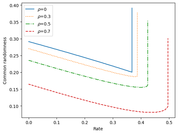
We provide in Fig. 2 the rate-common randomness region with different correlation values of $S$ and $S_{e}$ under distortion constraint $D=3$. The figure shows that a higher correlation value $\rho$ implies a higher communication rate and a lower common randomness rate, which is reasonable since a high correlation implies the side information $S_{e}$ at the sender side is highly related to the channel state $S$, and hence is helpful in both communication and state estimation. Also note that when $\rho=0$, the Gaussian random variables $S_{e}$ and $S$ are independent of each other, and the sender can not benefit from observing the side information. The right end of the solid line is the case when $\alpha=0$ (which is not the case with different values of $\rho$). The sender does not use the side information in both the communication and estimation which is implied by Fig. 2 to be optimal in this case since the correlation $\rho=0$.

IV Secure ISAC

In this section, we consider the distribution-preservation ISAC with private reconstruction requirement. Suppose there exists a henchman at the state estimator side and an eavesdropper who both observe the channel output $Y^{n}$. However, the eavesdropper does not have access to the common randomness. The henchman observes the reconstructed sequence and the sequences at the encoder side, it transmits a rate-limited message to the eavesdropper to help the eavesdropper reconstruct the state sequence.

There is an additional distortion constraint that the distortion between reconstructed sequences at the state estimator side and the receiver side is lower bounded by a given number $D_{E}$. Let $\mathcal{C}$ be the communication codebook used between the sender and receiver. The behavior of the henchman and eavesdropper is defined as follows.

Definition 3.

A henchman in an ISAC system observes the behavior of the encoder. Its operation consists of

  • โ€ข

    a message set $\mathcal{M}_{E}=[1:2^{nR_{E}}]$,

  • โ€ข

    an encoder $f_{E}:\hat{\mathcal{S}}^{n}\times\mathcal{Y}^{n}\times\mathcal{C}\to\mathcal{M}_{E}$,

  • โ€ข

    a decoder $g_{E}:\mathcal{Y}^{n}\times\mathcal{M}_{E}\times\mathcal{C}\to\hat{\mathcal{S}}_{E}^{n}$.

Definition 4.

Given real numbers $D\geq 0,D_{E}\geq 0,P\geq 0$, a CR-assisted code is $(D,D_{E},P)-$ achievable if for any $\epsilon>0$ and sufficiently large $n$, there exists an $(n,R,R_{c})$ code such that

Pโ€‹rโ€‹{Mโ‰ M^}โ‰คฯต,โ€–PS^nโˆ’ฯˆnโ€–โ‰คฮ”formulae-sequence๐‘ƒ๐‘Ÿ๐‘€^๐‘€italic-ฯตnormsubscript๐‘ƒsuperscript^๐‘†๐‘›superscript๐œ“๐‘›ฮ”\displaystyle Pr\{M\neq\hat{M}\}\leq\epsilon,\;||P_{\hat{S}^{n}}-\psi^{n}||\leq\Delta
$\displaystyle\mathbb{E}\left[d(S^{n},\hat{S}^{n})\right]\leq D,\;\mathbb{E}\left[d(\hat{S}^{n},\hat{S}^{n}_{E})\right]\geq D_{E}.$

The main result for this section is as follows.

Theorem 3.

(Inner bound) An inner bound of the secure CR-assisted distribution-preserving capacity-distortion region is

$$\begin{split}&C(D,D_{E},0)=\\ &\left\{\begin{aligned} &(R,R_{c})\in\mathbb{R}^{2}:R\geq 0,R_{c}\geq 0,\exists P_{S_{e}SUXYZ\hat{S}}\in\mathcal{P},\\ &R\leq I(U;Y)-I(U;S_{e}),\\ &R_{c}\geq\max\{I(U;\hat{S})-I(U;Y),0\},\\ &D\geq\mathbb{E}[d(S,\hat{S})],\\ &D_{E}\leq\left\{\begin{aligned} &D(R_{E},P_{\hat{S}Y})\quad\quad\quad\quad\quad\quad\quad\quad\quad\quad\;\;\;\;\;\;\;\text{if $R_{E}<R_{c},$}\\ &\min\{D(R_{E},P_{\hat{S}Y}),D(R_{E}-R_{c},P_{U\hat{S}Y})\}\quad\text{if $R_{E}\geq R_{c}.$}\end{aligned}\right.\end{aligned}\right.\end{split}$$

where $D(r,P_{U\hat{S}Y})$ is the rate-distortion function such that $r$ is the compression rate and $P_{U\hat{S}Y}$ is the joint distribution such that $\hat{S}$ is the source and $U$ and $Y$ are side information available at both sides. We set $D(r,P_{U\hat{S}Y})=\infty$ if $r<0$.

The eavesdropper observes the channel output $Y^{n}$ but does not have access to the common randomness. When $R_{E}>R_{c}$, the henchman can always use $R_{c}$ bits to describe the common randomness, and then with high probability, the eavesdropper can decode the message and obtain the codeword $U^{n}$. In this case, distortion $D(R_{E}-R_{c},P_{U\hat{S}Y})$, which is the distortion-rate function under joint distribution $P_{{U\hat{S}Y}}$ with $U$ and $Y$ being common side information, is achievable at the eavesdropper. When $R_{E}<R_{c}$, the eavesdropper ignores the codeword, and uses a lossy compression code with rate $R_{E}$ and $Y$ being the common side information at both sides.

Sketch of the proof: To prove the achievability, the sender still uses the random binning coding provided in Theorem 1. For the henchman-eavesdropper, the system is equivalent to the case that a codeword $U^{n}(M,I,\Gamma)$ is selected uniformly at random and produces two sequences, $\hat{S}^{n}$ and $Y^{n}$, through a discrete memoryless channel $P^{n}_{Y\hat{S}|U}$. The henchman observes $(\hat{S}^{n},Y^{n})$ and describes $\hat{S}^{n}$ with a limited rate, and the eavesdropper decoder observes $Y^{n}$. The system is an extended version of the model in [17] with additional side information at both sides. The optimal strategy for the henchman-eavesdropper is to use a deterministic decoder sEnโ€‹(ME,Yn)subscriptsuperscript๐‘ ๐‘›๐ธsubscript๐‘€๐ธsuperscript๐‘Œ๐‘›s^{n}_{E}(M_{E},Y^{n}) and an encoder $f_{E}$ that maps each pair of ($\hat{S}^{n},Y^{n})$ to an interim codeword $V^{n}\in\mathcal{C}_{V}$ that minimizes the expectation of the distortion and set $\hat{S}^{n}_{E}=V^{n}$. To show the distortion achieved at the eavesdropper, it is sufficient to prove Pโ€‹rCโ€‹{maxfE,๐’žVโกPโ€‹rโ€‹{dโ€‹(S^,s^Enโ€‹(ME,Yn))โ‰คD}>ฯ„n}โ†’0โ†’๐‘ƒsubscript๐‘ŸCsubscriptsubscript๐‘“๐ธsubscript๐’ž๐‘‰๐‘ƒ๐‘Ÿ๐‘‘^๐‘†subscriptsuperscript^๐‘ ๐‘›๐ธsubscript๐‘€๐ธsuperscript๐‘Œ๐‘›๐ทsubscript๐œ๐‘›0Pr_{\textbf{C}}\left\{\max_{f_{E},\mathcal{C}_{V}}Pr\{d(\hat{S},\hat{s}^{n}_{E}(M_{E},Y^{n}))\leq D\}>\tau_{n}\right\}\to 0 for sufficiently large $n$ and small $\tau_{n}.$ The subscript C represents the random codebook used by the sender and legitimate receiver. Let $m_{E}(v^{n})$ be the encoding result when $v^{n}\in\mathcal{C}_{V}$ is selected. It can be shown that

maxfE,๐’žVโกPโ€‹rโ€‹{dโ€‹(S^,s^Enโ€‹(ME,Yn))โ‰คD}subscriptsubscript๐‘“๐ธsubscript๐’ž๐‘‰๐‘ƒ๐‘Ÿ๐‘‘^๐‘†subscriptsuperscript^๐‘ ๐‘›๐ธsubscript๐‘€๐ธsuperscript๐‘Œ๐‘›๐ท\displaystyle\max_{f_{E},\mathcal{C}_{V}}Pr\{d(\hat{S},\hat{s}^{n}_{E}(M_{E},Y^{n}))\leq D\}
โ‰ค2nโ€‹REโ€‹maxvnโˆˆ๐’ฑnโกPโ€‹rโ€‹{dโ€‹(S^,s^Enโ€‹(mEโ€‹(vn),Yn))โ‰คD}absentsuperscript2๐‘›subscript๐‘…๐ธsubscriptsuperscript๐‘ฃ๐‘›superscript๐’ฑ๐‘›๐‘ƒ๐‘Ÿ๐‘‘^๐‘†subscriptsuperscript^๐‘ ๐‘›๐ธsubscript๐‘š๐ธsuperscript๐‘ฃ๐‘›superscript๐‘Œ๐‘›๐ท\displaystyle\leq 2^{nR_{E}}\max_{v^{n}\in\mathcal{V}^{n}}Pr\{d(\hat{S},\hat{s}^{n}_{E}(m_{E}(v^{n}),Y^{n}))\leq D\}

by considering the โ€˜worst caseโ€™ that the best $v^{n}$ for the henchman-eavesdropper is in the codebook and the factor $2^{nR_{E}}$ is the result of the union bound and the fact that given side information $Y^{n}$ there are at most $2^{nR_{E}}$ possible decoding results for the eavesdropper decoder. The problem reduces to determining the compression rate given fixed $v^{n}\in\mathcal{V}^{n}$ and distortion constraint $D$ when side information $Y^{n}$ is available at the decoder side. The details are provided in Appendix D.

The following capacity-distortion region result can be obtained when the main channel is deterministic.

Corollary 4.

(Capacity region) The CR-assisted secure distribution-preserving capacity-distortion region of the deterministic channel is

$$C(D,D_{E},0)=\left\{\begin{aligned} (R,0)\in\mathbb{R}^{2}:&R\geq 0,\exists P_{S_{e}SUXYZ\hat{S}}\in\mathcal{P}_{DE},\\ &R\leq H(Y|S_{e}),\\ &D\geq\mathbb{E}[d(S,\hat{S})],\\ &D_{E}\leq D(R_{E},P_{Y\hat{S}}).\end{aligned}\right.$$

The achievability proof follows by setting $U=Y$ in Theorem 3, which is valid by the deterministic property of the main channel. For the converse, the bound of $R$ and $D$ remain the same as in Corollary 2. To show the bound on $D_{E}$, we use an extended version of the type covering lemma ([18, Lemma 9.1]), which is presented in [17, Lemma 4]. For each joint type of $(\hat{S}^{n},Y^{n})$ there exists a code by the type covering lemma and the number of types is $(n+1)^{|\mathcal{S}||\mathcal{Y}|}$, which can be compressed with a negligible rate. The details are provided in Appendix E.

References

  • [1] P.ย Schwenteck, G.ย T. Nguyen, H.ย Boche, W.ย Kellerer, and F.ย H. Fitzek, โ€œ6G perspective of mobile network operators, manufacturers, and verticals,โ€ IEEE Networking Letters, vol.ย 5, no.ย 3, pp.ย 169โ€“173, Sep. 2023.
  • [2] G.ย P. Fettweis and H.ย Boche, โ€œ6G: The personal tactile internetโ€”and open questions for information theory,โ€ IEEE BITS the Information Theory Magazine, vol.ย 1, no.ย 1, pp.ย 71โ€“82, Sep. 2021.
  • [3] G.ย P. Fettweis and H.ย Boche, โ€œOn 6G and trustworthiness,โ€ Communications of the ACM, vol.ย 65, no.ย 4, pp.ย 48โ€“49, 2022.
  • [4] A.ย Sutivong, M.ย Chiang, T.ย M. Cover, and Y.-H. Kim, โ€œChannel capacity and state estimation for state-dependent gaussian channels,โ€ IEEE Transactions on Information Theory, vol.ย 51, no.ย 4, pp.ย 1486โ€“1495, 2005.
  • [5] Y.-H. Kim, A.ย Sutivong, and T.ย M. Cover, โ€œState amplification,โ€ IEEE Transactions on Information Theory, vol.ย 54, no.ย 5, pp.ย 1850โ€“1859, 2008.
  • [6] W.ย Zhang, S.ย Vedantam, and U.ย Mitra, โ€œJoint transmission and state estimation: A constrained channel coding approach,โ€ IEEE Transactions on Information Theory, vol.ย 57, no.ย 10, pp.ย 7084โ€“7095, 2011.
  • [7] M.ย Ahmadipour, M.ย Kobayashi, M.ย Wigger, and G.ย Caire, โ€œAn information-theoretic approach to joint sensing and communication,โ€ IEEE Transactions on Information Theory, vol.ย 70, no.ย 2, pp.ย 1124 โ€“ 1146, 2022.
  • [8] Y.ย Xiong, F.ย Liu, Y.ย Cui, W.ย Yuan, T.ย X. Han, and G.ย Caire, โ€œOn the fundamental tradeoff of integrated sensing and communications under gaussian channels,โ€ IEEE Transactions on Information Theory, vol.ย 69, no.ย 9, pp.ย 5723 โ€“ 5751, 2023.
  • [9] O.ย Gรผnlรผ, M.ย R. Bloch, R.ย F. Schaefer, and A.ย Yener, โ€œSecure integrated sensing and communication,โ€ IEEE Journal on Selected Areas in Information Theory, vol.ย 4, pp.ย 40โ€“53, 2023.
  • [10] O.ย Gรผnlรผ, M.ย Bloch, R.ย F. Schaefer, and A.ย Yener, โ€œSecure integrated sensing and communication for binary input additive white gaussian noise channels,โ€ in 2023 IEEE 3rd International Symposium on Joint Communications & Sensing (JC&S), pp.ย 1โ€“6, IEEE, 2023.
  • [11] A.ย B. Wagner, โ€œThe rate-distortion-perception tradeoff: The role of common randomness,โ€ arXiv preprint arXiv:2202.04147, 2022.
  • [12] J.ย Chen, L.ย Yu, J.ย Wang, W.ย Shi, Y.ย Ge, and W.ย Tong, โ€œOn the rate-distortion-perception function,โ€ IEEE Journal on Selected Areas in Information Theory, vol.ย 3, no.ย 4, pp.ย 664โ€“673, 2022.
  • [13] N.ย Saldi, T.ย Linder, and S.ย Yรผksel, โ€œOutput constrained lossy source coding with limited common randomness,โ€ IEEE Transactions on Information Theory, vol.ย 61, no.ย 9, pp.ย 4984โ€“4998, 2015.
  • [14] Z.ย Goldfeld, P.ย Cuff, and H.ย Permuter, โ€œWiretap channels with random states non-causally available at the encoder,โ€ IEEE Transactions on Information Theory, vol.ย 66, no.ย 3, pp.ย 1497โ€“1519, 2019.
  • [15] E.ย C. Song, P.ย Cuff, and H.ย V. Poor, โ€œThe likelihood encoder for lossy compression,โ€ IEEE Transactions on Information Theory, vol.ย 62, no.ย 4, pp.ย 1836โ€“1849, 2016.
  • [16] A.ย Elย Gamal and Y.-H. Kim, Network Information Theory. Cambridge University Press, 2011.
  • [17] C.ย Schieler and P.ย Cuff, โ€œThe henchman problem: Measuring secrecy by the minimum distortion in a list,โ€ IEEE Transactions on Information Theory, vol.ย 62, no.ย 6, pp.ย 3436โ€“3450, 2016.
  • [18] I.ย Csiszรกr and J.ย Kรถrner, Information Theory: Coding Theorems for Discrete Memoryless Systems. Cambridge University Press, 2011.
  • [19] C.ย E. Shannon, โ€œChannels with side information at the transmitter,โ€ IBM Journal of Research and Development, vol.ย 2, no.ย 4, pp.ย 289โ€“293, 1958.
  • [20] C.ย Villani etย al., Optimal transport: old and new, vol.ย 338. Springer, 2009.

Appendix A coding scheme for theorem 1

In this section, we prove the achievability of Theorem 1.

Before giving the decoding error and distortion analysis, we first state two properties of total variation as follows.

Lemma 1.

[15, Property 1] Given alphabet $\mathcal{X}$ and distributions $P$ and $Q$ on $\mathcal{X}$, the following statements hold:

  1. (a)

    Let $\epsilon>0$ and $f(x)$ be a function in a bounded range with width $b\in\mathbb{R}^{+}$. It follows that

    $\displaystyle||P-Q||<\epsilon\Rightarrow|\mathbb{E}_{P}\left[f(X)\right]-\mathbb{E}_{Q}\left[f(X)\right]|\leq b\epsilon.$
  2. (b)

    Let $P_{X}P_{Y|X}$ and $Q_{X}P_{Y|X}$ be joint distributions on $\mathcal{X}\times\mathcal{Y}$. It follows that

    $\displaystyle||P_{X}P_{Y|X}-Q_{X}P_{Y|X}||=||P_{X}-Q_{X}||.$

We first analyze the decoding error induced by distribution $Q$, then by the property of total variation Lemma 1(a), the error probability induced by another close distribution $\bar{Q}$ can also be bounded. Define the following error events and suppose $(M,I,\Gamma)=(1,1,\gamma)$

$\displaystyle\mathcal{E}_{1}=\{(U^{n}(1,1,\gamma),Y^{n})\notin T^{n}_{P_{UY},\delta}\},$
โ„ฐ2={(Unโ€‹(mโ€ฒ,iโ€ฒ,ฮณ),Yn)โˆˆTPUโ€‹Y,ฮดnโ€‹for someย (mโ€ฒ,iโ€ฒ)โ‰ (1,1)}.subscriptโ„ฐ2superscript๐‘ˆ๐‘›superscript๐‘šโ€ฒsuperscript๐‘–โ€ฒ๐›พsuperscript๐‘Œ๐‘›subscriptsuperscript๐‘‡๐‘›subscript๐‘ƒ๐‘ˆ๐‘Œ๐›ฟfor someย (mโ€ฒ,iโ€ฒ)โ‰ (1,1)\displaystyle\mathcal{E}_{2}=\{(U^{n}(m^{\prime},i^{\prime},\gamma),Y^{n})\in T^{n}_{P_{UY},\delta}\;\text{for some $(m^{\prime},i^{\prime})\neq(1,1)$}\}.

By standard joint typicality argument for Gelโ€™fand-Pinsker coding, under distribution $Q$ the decoding error probability is bounded by

Pโ€‹rQโ€‹{Mโ‰ M^}โ†’0โ†’๐‘ƒsubscript๐‘Ÿ๐‘„๐‘€^๐‘€0\displaystyle Pr_{Q}\{M\neq\hat{M}\}\to 0

if $R+R_{p}\leq I(U;Y)$. The remaining analysis relies on the following soft-covering lemma.

Lemma 2.

Let $(U,V)\in\mathcal{U}\times\mathcal{V}$ be a pair of random variables with joint distribution $P_{UV}$. Let $\textbf{C}=\{U^{n}(i):i\in[1:2^{nR}]\}$ be a random collection of sequences $U^{n}(i)$, each i.i.d. generated by $P_{U}^{n}$. We denote the sample value of C by $\mathcal{C}$. Let $P_{V}$ be the underlying marginal distribution of $V$ induced by joint distribution $P_{UV}$ and define the output distribution induced by random codebook C as

$\displaystyle Q_{V^{n}}(v^{n})=\frac{1}{|\text{C}|}\sum_{i=1}^{2^{nR}}P_{V^{n}|U^{n}}(v^{n}|U^{n}(i)),\;\;\text{for any $v^{n}\in\mathcal{V}^{n}$},$

where $P_{V^{n}|U^{n}}=\prod_{i=1}^{n}P_{V|U}$. If $R>I(U;V)$, we have

$\displaystyle\mathbb{E}_{\textbf{C}}\left[||Q_{V^{n}}-P_{V}^{n}||_{TV}\right]\leq\frac{3}{2}exp\{-\kappa n\}$

for some $\kappa>0$.

Now invoking Lemma 2, we have

$\displaystyle\mathbb{E}_{\textbf{C}(m,\gamma)}\left[||Q_{S^{n}_{e}|M=m,\Gamma=\gamma}-P^{n}_{S_{e}}||\right]\leq\frac{3}{2}exp\{-an\}$

for some $a>0$ if $R_{p}>I(U;S_{e})$, and hence,

$\displaystyle\mathbb{E}_{\textbf{C}}\left[||Q_{M\Gamma S^{n}_{e}}-\frac{1}{2^{n(R+R_{c})}}P^{n}_{S_{e}}||\right]\leq\frac{3}{2}\exp\{-an\},$

which gives us

$\displaystyle\mathbb{E}_{\textbf{C}}\left[||Q_{MI\Gamma S^{n}_{e}S^{n}X^{n}Y^{n}Z^{n}\hat{S}^{n}}-\bar{Q}_{MI\Gamma S^{n}_{e}S^{n}X^{n}Y^{n}Z^{n}\hat{S}^{n}}||\right]$
$\displaystyle=\mathbb{E}_{\textbf{C}}\left[||Q_{M\Gamma S^{n}_{e}}-\bar{Q}_{M\Gamma S^{n}_{e}}||\right]$
$\displaystyle=\mathbb{E}_{\textbf{C}}\left[||Q_{M\Gamma S^{n}_{e}}-\frac{1}{2^{n(R+R_{c})}}P^{n}_{S_{e}}||\right]\leq\frac{3}{2}\exp\{-an\}$ (8)

by Lemma 1(b). For a given random codebook $\mathbf{C}$, define function g๐‚โ€‹(m,m^)=๐•€โ€‹{mโ‰ m^}subscript๐‘”๐‚๐‘š^๐‘š๐•€๐‘š^๐‘šg_{\mathbf{C}}(m,\hat{m})=\mathbb{I}\{m\neq\hat{m}\}. Now follow the same argument as [14, Eq. (41)-(44)] with Lemma 1(a) we have

Pโ€‹rQยฏโ€‹{Mโ‰ M^}โ‰คฯตโ‹…32โ€‹expโก{โˆ’aโ€‹n}โ†’0โ€‹asโ€‹nโ†’โˆž๐‘ƒsubscript๐‘Ÿยฏ๐‘„๐‘€^๐‘€โ‹…italic-ฯต32๐‘Ž๐‘›โ†’0as๐‘›โ†’\displaystyle Pr_{\bar{Q}}\{M\neq\hat{M}\}\leq\epsilon\cdot\frac{3}{2}\exp\{-an\}\to 0\;\;\text{as}\;\;n\to\infty (9)

On the other hand, by setting $R+R_{p}+R_{c}>I(U;\hat{S})$ and applying Lemma 2, we have

$\displaystyle\mathbb{E}_{\textbf{C}}\left[||Q_{\hat{S}^{n}}-P_{\hat{S}}^{n}||\right]$
$\displaystyle=\mathbb{E}_{\textbf{C}}\left[||Q_{\hat{S}^{n}}-P_{S}^{n}||\right]\leq\frac{3}{2}\exp\{-bn\}$

for some $b>0$. By the triangle inequality property of the total variation [15, Property 1(c)], we have

$\displaystyle\mathbb{E}_{\textbf{C}}\left[||\bar{Q}_{\hat{S}^{n}}-P_{S}^{n}||\right]$
$\displaystyle\leq\mathbb{E}_{\textbf{C}}\left[||\bar{Q}_{\hat{S}^{n}}-Q_{\hat{S}^{n}}||\right]+\mathbb{E}_{\textbf{C}}\left[||Q_{\hat{S}^{n}}-P_{S}^{n}||\right]$
$\displaystyle\leq\frac{3}{2}\exp\{-an\}+\frac{3}{2}\exp\{-bn\}:=\frac{3}{2}\exp\{-cn\}$ (10)

for some $c>0$. For the reconstruction distortion part, we first consider the distortion under distribution $Q$ and define additional error events

$\displaystyle\mathcal{E}_{3}=\{(U^{n}(1,1,\gamma),S^{n}_{e},S^{n})\notin T^{n}_{P_{US_{e}S},\delta}\},$
$\displaystyle\mathcal{E}_{4}=\{(X^{n},S^{n}_{e},Z^{n},\hat{S}^{n})\notin T^{n}_{P_{XS_{e}Z\hat{S}},\delta}\}$

We say a distortion error $\mathcal{E}_{d}$ occurs if at least one of the events $\mathcal{E}_{1},\mathcal{E}_{2},\mathcal{E}_{3}$ and $\mathcal{E}_{4}$ happens. By the law of large numbers, it follows that $Pr\{\mathcal{E}_{3}\}\to 0$ and $Pr\{\mathcal{E}_{4}\}\to 0$ as $n\to\infty$ and then $P_{d,e}:=Pr\{\mathcal{E}_{d}\}\to 0$ follows. The expectation of the distortion (taken over random codebook, random states and random channel noise) under distribution $Q$ is bounded by

$\displaystyle\mathbb{E}\left[d(S^{n},\hat{S}^{n})\right]$
$\displaystyle=(1-P_{d,e})\mathbb{E}\left[d(S^{n},\hat{S}^{n})|\mathcal{E}_{d}^{c}\right]+P_{d,e}\mathbb{E}\left[d(S^{n},\hat{S}^{n})|\mathcal{E}_{d}\right]$
$\displaystyle\overset{(a)}{\leq}(1-P_{d,e})\mathbb{E}_{\textbf{C}}\left[\sum_{s^{n},\hat{s}^{n}}d(s^{n},\hat{s}^{n})\right.$
$\displaystyle\left.\sum_{\begin{subarray}{c}m,i,\gamma,s^{n}_{e},\\ x^{n},y^{n},z^{n}\end{subarray}}Q_{MI\Gamma S^{n}_{e}S^{n}X^{n}Y^{n}Z^{n}\hat{S}^{n}}(m,i,\gamma,s^{n}_{e},s^{n},x^{n},y^{n},z^{n},\hat{s}^{n})\right]$
$\displaystyle\quad\quad\quad\quad\quad\quad\quad\quad+P_{d,e}D_{max}$
โ‰ค(1โˆ’Pd,e)โ€‹โˆ‘sn,s^ndโ€‹(sn,s^n)absent1subscript๐‘ƒ๐‘‘๐‘’subscriptsuperscript๐‘ ๐‘›superscript^๐‘ ๐‘›๐‘‘superscript๐‘ ๐‘›superscript^๐‘ ๐‘›\displaystyle\leq(1-P_{d,e})\sum_{s^{n},\hat{s}^{n}}d(s^{n},\hat{s}^{n})
๐”ผCโ€‹[โˆ‘m,i,ฮณ,sen,xn,yn,znQMโ€‹Iโ€‹ฮ“โ€‹Senโ€‹Snโ€‹Xnโ€‹Ynโ€‹Znโ€‹S^nโ€‹(m,i,ฮณ,sen,sn,xn,yn,zn,s^n)]subscript๐”ผCdelimited-[]subscript๐‘š๐‘–๐›พsubscriptsuperscript๐‘ ๐‘›๐‘’superscript๐‘ฅ๐‘›superscript๐‘ฆ๐‘›superscript๐‘ง๐‘›subscript๐‘„๐‘€๐ผฮ“subscriptsuperscript๐‘†๐‘›๐‘’superscript๐‘†๐‘›superscript๐‘‹๐‘›superscript๐‘Œ๐‘›superscript๐‘๐‘›superscript^๐‘†๐‘›๐‘š๐‘–๐›พsubscriptsuperscript๐‘ ๐‘›๐‘’superscript๐‘ ๐‘›superscript๐‘ฅ๐‘›superscript๐‘ฆ๐‘›superscript๐‘ง๐‘›superscript^๐‘ ๐‘›\displaystyle\quad\mathbb{E}_{\textbf{C}}\left[\sum_{\begin{subarray}{c}m,i,\gamma,s^{n}_{e},\\ x^{n},y^{n},z^{n}\end{subarray}}Q_{MI\Gamma S^{n}_{e}S^{n}X^{n}Y^{n}Z^{n}\hat{S}^{n}}(m,i,\gamma,s^{n}_{e},s^{n},x^{n},y^{n},z^{n},\hat{s}^{n})\right]
$\displaystyle\quad\quad\quad\quad\quad\quad\quad\quad+P_{d,e}D_{max}$
=(b)โ€‹(1โˆ’Pd,e)โ€‹โˆ‘sn,s^ndโ€‹(sn,s^n)โ€‹PSโ€‹S^nโ€‹(sn,s^n)+Pd,eโ€‹Dmโ€‹aโ€‹x๐‘1subscript๐‘ƒ๐‘‘๐‘’subscriptsuperscript๐‘ ๐‘›superscript^๐‘ ๐‘›๐‘‘superscript๐‘ ๐‘›superscript^๐‘ ๐‘›subscriptsuperscript๐‘ƒ๐‘›๐‘†^๐‘†superscript๐‘ ๐‘›superscript^๐‘ ๐‘›subscript๐‘ƒ๐‘‘๐‘’subscript๐ท๐‘š๐‘Ž๐‘ฅ\displaystyle\overset{(b)}{=}(1-P_{d,e})\sum_{s^{n},\hat{s}^{n}}d(s^{n},\hat{s}^{n})P^{n}_{S\hat{S}}(s^{n},\hat{s}^{n})+P_{d,e}D_{max}
$\displaystyle\leq(1-P_{d,e})D+P_{d,e}D_{max},$

where $(a)$ follows by the fact that $\mathcal{E}_{d}^{c}$ implies the correct decoding, $(b)$ follows by the definition of $\mathcal{P}(D,P)$. To bound the true distortion (distortion under distribution $\hat{Q}$), we invoke Lemma 1(a) again and it follows that

$\displaystyle|\mathbb{E}_{\hat{Q}}[d(S^{n},\hat{S}^{n})]-\mathbb{E}_{Q}[d(S^{n},\hat{S}^{n})]|$
$\displaystyle\leq D_{max}||Q_{S^{n}\hat{S}^{n}}-\hat{Q}_{S^{n}\hat{S}^{n}}||$
$\displaystyle\leq D_{max}||Q_{MI\Gamma S^{n}_{e}S^{n}X^{n}Y^{n}Z^{n}\hat{S}^{n}}-\bar{Q}_{MI\Gamma S^{n}_{e}S^{n}X^{n}Y^{n}Z^{n}\hat{S}^{n}}||$
$\displaystyle\leq D_{max}\frac{3}{2}\exp\{-an\}.$

With sufficiently large block length $n$, we have

$\displaystyle\mathbb{E}_{\hat{Q}}[d(S^{n},\hat{S}^{n})]\leq D.$

So far, we have proved the achievability of region $C(D,\frac{3}{2}\exp\{-cn\})$. The proof is completed by using an optimal transportation argument as done in [13]. Let $T_{\hat{S}^{{}^{\prime}n}|\hat{S}^{n}}$ be a conditional distribution that convert random sequence $\hat{S}^{n}$ to $\hat{S}^{{}^{\prime}n}$. The argument shows that when the total variation of the distributions of $\hat{S}^{n}$ and $\hat{S}^{{}^{\prime}n}$ is close, one can construct a random sequence $\hat{S}^{{}^{\prime}n}$ such that $P_{\hat{S}^{{}^{\prime}n}}=\psi^{n}$ with an additional distortion that decays exponentially fast with the block length $n$, and the term $T_{\hat{S}^{{}^{\prime}n}|\hat{S}^{n}}$ is called the optimal coupling. For completeness, we provide the argument in Appendix C. This completes the achievability proof.

Appendix B proof of theorem 2

In this section, we prove the converse part of Theorem 2. Note that the reliable communication over the channel is equivalent to considering a channel PYโ€‹Z|Xโ€‹Seโ€‹(y,z|x,se)=โˆ‘sPYโ€‹Z|Xโ€‹Sโ€‹(y,z|x,s)โ€‹PS|Seโ€‹(s|se)subscript๐‘ƒconditional๐‘Œ๐‘๐‘‹subscript๐‘†๐‘’๐‘ฆconditional๐‘ง๐‘ฅsubscript๐‘ ๐‘’subscript๐‘ subscript๐‘ƒconditional๐‘Œ๐‘๐‘‹๐‘†๐‘ฆconditional๐‘ง๐‘ฅ๐‘ subscript๐‘ƒconditional๐‘†subscript๐‘†๐‘’conditional๐‘ subscript๐‘ ๐‘’P_{YZ|XS_{e}}(y,z|x,s_{e})=\sum_{s}P_{YZ|XS}(y,z|x,s)P_{S|S_{e}}(s|s_{e}). The bound on $R$ follows similarly to the converse proof of channel with causal side information[19].

$\displaystyle nR$ $\displaystyle=H(M)$
$\displaystyle\leq I(M;Y^{n})$
$\displaystyle=\sum_{i=1}^{n}I(M;Y_{i}|Y^{i-1})$
$\displaystyle\leq\sum_{i=1}^{n}I(M,\Gamma,S_{e}^{i-1},X^{i-1},Y^{i-1};Y_{i})$
$\displaystyle\overset{(a)}{=}\sum_{i=1}^{n}I(M,\Gamma,S_{e}^{i-1},X^{i-1};Y_{i})$
$\displaystyle\overset{(b)}{=}\sum_{i=1}^{n}I(M,\Gamma,S_{e}^{i-1};Y_{i})$
$\displaystyle\overset{(c)}{=}n\cdot\frac{1}{n}\sum_{i=1}^{n}I(M,\Gamma,S_{e}^{Q-1};Y_{Q}|Q=i)\overset{(d)}{=}nI(U;Y)$

where $(a)$ follows by the Markov chain $Y_{i}-(S_{e}^{i-1},X^{i-1})-Y^{i-1}$, $(b)$ follows by the fact that $X^{i-1}$ is a deterministic function of $(M,\Gamma,S^{i-1}_{e})$, $(c)$ follows by introducing a time-sharing random variable $Q\in[1,\dots,n]$, $d$ follows by setting $U_{Q}=(M,\Gamma,S_{e}^{Q-1}),U=(U_{Q},Q),Y=Y_{Q}$.

For the sum rate, it follows that

$\displaystyle n(R+R_{c})$ $\displaystyle\geq H(M,\Gamma)$
$\displaystyle\geq I(M,\Gamma;S^{n}_{e},\hat{S}^{n})$
$\displaystyle=\sum_{i=1}^{n}I(M,\Gamma;S_{e,i},\hat{S}_{i}|S_{e}^{i-1},\hat{S}^{i-1})$
$\displaystyle\overset{(a)}{=}\sum_{i=1}^{n}I(M,\Gamma,S_{e}^{i-1},\hat{S}^{i-1};S_{e,i},\hat{S}_{i})$
$\displaystyle\geq\sum_{i=1}^{n}I(M,\Gamma,S_{e}^{i-1};S_{e,i},\hat{S}_{i})$
$\displaystyle=n\cdot\frac{1}{n}\sum_{i=1}^{n}I(U_{Q};S_{e,Q},\hat{S}_{Q}|Q=i)$
$\displaystyle\overset{(b)}{=}nI(U_{Q},Q;S_{e,Q},\hat{S}_{Q})=nI(U;S_{e},\hat{S}).$

where $(a)$ follows by the i.i.d. property of $(S_{e,i},\hat{S}_{i}),i=1,2,\dots$, $(b)$ follows by the independence between $Q$ and $(S_{e,Q},\hat{S}_{Q})$.

Appendix C optimal transport argument

In this section we provide the explanation of the optimal transport argument in Appendix A, which is a direct application of the argument in [13] to our model. Given a cost function $c(S^{n},\hat{S}^{n})$ such that $c:S^{n}\times\hat{S}^{n}\to[0,+\infty)$ is a matric on $\mathcal{S}^{n}=\hat{\mathcal{S}}^{n}$, the optimal transportation is defined by

$\displaystyle\hat{T}_{n}(P_{\hat{S}^{n}},P_{S}^{n})=\inf\{\mathbb{E}\left[c(S^{n},\hat{S}^{n})\right]:S^{n}\sim P_{S}^{n},\;\hat{S}^{n}\sim P_{\hat{S}^{n}}\},$ (11)

where the infimum is taken over all joint distributions $P_{S^{n}\hat{S}^{n}}$ giving marginal distributions defined in (11). The distribution giving the infimum in (11) is called the optimal coupling of $P_{\hat{S}^{n}}$ and $P_{S}^{n}$. We follow the convention in [13] and call the corresponding conditional distribution of $S^{n}$ given $\hat{S}^{n}$ an optimal coupling as well, denoted by $T_{\hat{S}^{{}^{\prime}n}|\hat{S}^{n}}$. Note that given the distortion function one can further define

$\displaystyle\rho_{n}(S^{n},\hat{S}^{n})=(\sum_{i=1}^{n}d(S_{i},\hat{S}_{i})^{p})^{\frac{1}{q}},$

which is also a metric on $\mathcal{S}^{n}$. In our case, we have $p=q=1$. However, the arguments can be extended to more general positive $p=q\geq 1$. It follows that

$\displaystyle\hat{T}_{n}(P_{\hat{S}^{n}},P_{S}^{n})$
$\displaystyle=\inf\{\mathbb{E}\left[d(S^{n},\hat{S}^{n})\right]:S^{n}\sim P_{S}^{n},\;\hat{S}^{n}\sim P_{\hat{S}^{n}}\}$
$\displaystyle=\frac{1}{n}\inf\left\{\mathbb{E}\left[\sum_{i=1}^{n}d(S_{i},\hat{S}_{i})^{p}\right]^{\frac{1}{q}}:S^{n}\sim P_{S}^{n},\;\hat{S}^{n}\sim P_{\hat{S}^{n}}\right\}^{q}$
$\displaystyle=\frac{1}{n}(W_{q}(P_{\hat{S}^{n}},P_{S}^{n}))^{q},$

where $W_{q}$ is the Wasserstein distance of order $q$ with cost function $\rho_{n}$. Using [20, Theorem 6.15] and [20, Particular Case 6.16] we have

$\displaystyle W_{q}(P_{\hat{S}^{n}},P_{S}^{n})$ โ‰ค21qโ€ฒโ€‹(โˆ‘snฯnqโ€‹(s0n,sn)โ€‹|PS^nโ€‹(sn)โˆ’PSnโ€‹(sn)|)1qabsentsuperscript21superscript๐‘žโ€ฒsuperscriptsubscriptsuperscript๐‘ ๐‘›superscriptsubscript๐œŒ๐‘›๐‘žsubscriptsuperscript๐‘ ๐‘›0superscript๐‘ ๐‘›subscript๐‘ƒsuperscript^๐‘†๐‘›superscript๐‘ ๐‘›superscriptsubscript๐‘ƒ๐‘†๐‘›superscript๐‘ ๐‘›1๐‘ž\displaystyle\leq 2^{\frac{1}{q^{\prime}}}\left(\sum_{s^{n}}\rho_{n}^{q}(s^{n}_{0},s^{n})|P_{\hat{S}^{n}}(s^{n})-P_{S}^{n}(s^{n})|\right)^{\frac{1}{q}}
=21qโ€ฒโ€‹(โˆ‘snโˆ‘i=1ndโ€‹(s0,i,si)pโ€‹|PS^nโ€‹(sn)โˆ’PSnโ€‹(sn)|)1qabsentsuperscript21superscript๐‘žโ€ฒsuperscriptsubscriptsuperscript๐‘ ๐‘›superscriptsubscript๐‘–1๐‘›๐‘‘superscriptsubscript๐‘ 0๐‘–subscript๐‘ ๐‘–๐‘subscript๐‘ƒsuperscript^๐‘†๐‘›superscript๐‘ ๐‘›superscriptsubscript๐‘ƒ๐‘†๐‘›superscript๐‘ ๐‘›1๐‘ž\displaystyle=2^{\frac{1}{q^{\prime}}}\left(\sum_{s^{n}}\sum_{i=1}^{n}d(s_{0,i},s_{i})^{p}|P_{\hat{S}^{n}}(s^{n})-P_{S}^{n}(s^{n})|\right)^{\frac{1}{q}}
$\displaystyle\leq D_{max}||P_{\hat{S}^{n}}-P_{S}^{n}||\leq D_{max}\frac{3}{2}\exp\{-cn\}.$ (12)

for some $c>0$ and $q^{\prime}$ such that $\frac{1}{q^{\prime}}+\frac{1}{q}=1$. Now we apply the optimal coupling $T_{\hat{S}^{n^{\prime}}|\hat{S}^{n}}$ to the reconstructed sequence $\hat{S}^{n}$. By the triangle inequality of a metric we can bound the distortion as

$\displaystyle\left(\mathbb{E}\left[(\frac{1}{n}\sum_{i=1}^{n}d(S_{i},\hat{S}_{i}^{\prime})^{p})\right]\right)^{\frac{1}{q}}$
$\displaystyle\leq\left(\mathbb{E}\left[(\frac{1}{n}\sum_{i=1}^{n}d(S_{i},\hat{S}_{i})^{p})\right]\right)^{\frac{1}{q}}+\left(\mathbb{E}\left[(\frac{1}{n}\sum_{i=1}^{n}d(\hat{S}_{i},\hat{S}_{i}^{\prime})^{p})\right]\right)^{\frac{1}{q}}$
$\displaystyle\overset{(a)}{=}\mathbb{E}[d^{n}(S^{n},\hat{S}^{n})]+\hat{T}_{n}(P_{\hat{S}^{n}},P_{S}^{n})\leq D+\delta,$

where $(a)$ follows by settig $p=q=1$, $(b)$ follows by Appendix A and (12). The proof is completed.

Appendix D proof of theorem 3

We first consider the system induced by the idealized distribution defined in (3) in Appendix A. The distribution $P_{Y^{n}\hat{S}^{n}|U^{n}}$ is the same as considering the distribution $P_{X^{n}S_{e}^{n}Y^{n}\hat{S}^{n}|U^{n}}$ with additional side information $X^{n},S^{n}_{e}$ at the encoder side. Since the decoder only observes the side information $Y^{n}$, considering $(U^{n},Y^{n},\hat{S}^{n})$ is sufficient for the analysis.

We first argue for the best strategy for the henchman-eavesdropper. For a given henchman encoder $f_{E}$, suppose the decoder is a stochastic decoder that maps each description $m_{E}\in[1:2^{nR_{E}}]$ to a sequence $\hat{S}_{E}^{n}\in\mathcal{S}^{n}$. Then, there exists a minimizer achieving a smaller distortion by choosing the s^Ensuperscriptsubscript^๐‘ ๐ธ๐‘›\hat{s}_{E}^{n} that minimizes the expectation of the distortion among all possible choices for each $m_{E}$, that is

gโ€‹(mE,yn)=argโกmins^Enโˆˆ๐’ฎn๐”ผโ€‹[dโ€‹(S^n,s^En)].๐‘”subscript๐‘š๐ธsuperscript๐‘ฆ๐‘›subscriptsubscriptsuperscript^๐‘ ๐‘›๐ธsuperscript๐’ฎ๐‘›๐”ผdelimited-[]๐‘‘superscript^๐‘†๐‘›subscriptsuperscript^๐‘ ๐‘›๐ธ\displaystyle g(m_{E},y^{n})=\mathop{\arg\min}_{\hat{s}^{n}_{E}\in\mathcal{S}^{n}}\mathbb{E}\left[d(\hat{S}^{n},\hat{s}^{n}_{E})\right].

Hence, randomization does not help and the decoder of the eavesdropper is a deterministic decoder. Given an encoder $f_{E}$ such that $f_{E}(\hat{S}^{n},Y^{n})=M_{E}\in[1:2^{nR_{E}}]$ and side information $y^{n}\in\mathcal{Y}^{n}$, the decoder maps each $m_{E}$ to a unique reconstruction sequence with the help of side information $Y^{n}$. Without loss of generality, we can assume there exists an interim communication codebook $\mathcal{C}_{V}=\{v^{n}\}$, and given $Y^{n}$, the encoder maps each $m_{E}$ to a unique codeword in this interim codebook such that the eavesdropper can recover the interim codeword $V^{n}$ based on $M_{E}$ and $Y^{n}$. The reconstructed sequence is then determined by s^Enโ€‹(ME,Yn)=vnsubscriptsuperscript^๐‘ ๐‘›๐ธsubscript๐‘€๐ธsuperscript๐‘Œ๐‘›superscript๐‘ฃ๐‘›\hat{s}^{n}_{E}(M_{E},Y^{n})=v^{n}. The optimal encoder in this case selects the codeword in the interim communication codebook that minimizes ๐”ผโ€‹[dโ€‹(S^,s^Enโ€‹(ME,Yn))]๐”ผdelimited-[]๐‘‘^๐‘†subscriptsuperscript^๐‘ ๐‘›๐ธsubscript๐‘€๐ธsuperscript๐‘Œ๐‘›\mathbb{E}[d(\hat{S},\hat{s}^{n}_{E}(M_{E},Y^{n}))] and sends its description $M_{E}$ such that the decoder can locate the codeword with the help of the side information.

The above argument turns the problem into a henchman problem for lossy communication with additional side information at the henchman and eavesdropper sides. Given a random communication codebook C, common randomness rate $R_{c}$ and a distortion value $D$, we now bound the distortion expectation ๐”ผCโ€‹[๐”ผโ€‹[dโ€‹(S^,s^Enโ€‹(ME,Yn))]]subscript๐”ผCdelimited-[]๐”ผdelimited-[]๐‘‘^๐‘†subscriptsuperscript^๐‘ ๐‘›๐ธsubscript๐‘€๐ธsuperscript๐‘Œ๐‘›\mathbb{E}_{\textbf{C}}\left[\mathbb{E}[d(\hat{S},\hat{s}^{n}_{E}(M_{E},Y^{n}))]\right]. It follows that

minfE,๐’žVโก๐”ผโ€‹[dโ€‹(S^,s^Enโ€‹(ME,Yn))]subscriptsubscript๐‘“๐ธsubscript๐’ž๐‘‰๐”ผdelimited-[]๐‘‘^๐‘†subscriptsuperscript^๐‘ ๐‘›๐ธsubscript๐‘€๐ธsuperscript๐‘Œ๐‘›\displaystyle\min_{f_{E},\mathcal{C}_{V}}\mathbb{E}[d(\hat{S},\hat{s}^{n}_{E}(M_{E},Y^{n}))]
=minfE,๐’žVโก๐”ผโ€‹[dโ€‹(S^,s^Enโ€‹(ME,Yn))โ€‹|dโ€‹(S^,s^Enโ€‹(ME,Yn))>โ€‹D]absentsubscriptsubscript๐‘“๐ธsubscript๐’ž๐‘‰๐”ผdelimited-[]๐‘‘^๐‘†subscriptsuperscript^๐‘ ๐‘›๐ธsubscript๐‘€๐ธsuperscript๐‘Œ๐‘›ket๐‘‘^๐‘†subscriptsuperscript^๐‘ ๐‘›๐ธsubscript๐‘€๐ธsuperscript๐‘Œ๐‘›๐ท\displaystyle=\min_{f_{E},\mathcal{C}_{V}}\mathbb{E}[d(\hat{S},\hat{s}^{n}_{E}(M_{E},Y^{n}))|d(\hat{S},\hat{s}^{n}_{E}(M_{E},Y^{n}))>D]
โ‹…Pโ€‹rโ€‹{dโ€‹(S^,s^Enโ€‹(ME,Yn))>D}โ‹…absent๐‘ƒ๐‘Ÿ๐‘‘^๐‘†subscriptsuperscript^๐‘ ๐‘›๐ธsubscript๐‘€๐ธsuperscript๐‘Œ๐‘›๐ท\displaystyle\quad\quad\quad\quad\quad\cdot Pr\{d(\hat{S},\hat{s}^{n}_{E}(M_{E},Y^{n}))>D\}
+๐”ผโ€‹[dโ€‹(S^,s^Enโ€‹(ME,Yn))|dโ€‹(S^,s^Enโ€‹(ME,Yn))โ‰คD]๐”ผdelimited-[]conditional๐‘‘^๐‘†subscriptsuperscript^๐‘ ๐‘›๐ธsubscript๐‘€๐ธsuperscript๐‘Œ๐‘›๐‘‘^๐‘†subscriptsuperscript^๐‘ ๐‘›๐ธsubscript๐‘€๐ธsuperscript๐‘Œ๐‘›๐ท\displaystyle\quad\quad+\mathbb{E}[d(\hat{S},\hat{s}^{n}_{E}(M_{E},Y^{n}))|d(\hat{S},\hat{s}^{n}_{E}(M_{E},Y^{n}))\leq D]
โ‹…Pโ€‹rโ€‹{dโ€‹(S^,s^Enโ€‹(ME,Yn))โ‰คD}โ‹…absent๐‘ƒ๐‘Ÿ๐‘‘^๐‘†subscriptsuperscript^๐‘ ๐‘›๐ธsubscript๐‘€๐ธsuperscript๐‘Œ๐‘›๐ท\displaystyle\quad\quad\quad\quad\quad\cdot Pr\{d(\hat{S},\hat{s}^{n}_{E}(M_{E},Y^{n}))\leq D\}
โ‰ฅminfE,๐’žVโกDโ‹…Pโ€‹rโ€‹{dโ€‹(S^,s^Enโ€‹(ME,Yn))>D}.absentsubscriptsubscript๐‘“๐ธsubscript๐’ž๐‘‰โ‹…๐ท๐‘ƒ๐‘Ÿ๐‘‘^๐‘†subscriptsuperscript^๐‘ ๐‘›๐ธsubscript๐‘€๐ธsuperscript๐‘Œ๐‘›๐ท\displaystyle\geq\min_{f_{E},\mathcal{C}_{V}}D\cdot Pr\{d(\hat{S},\hat{s}^{n}_{E}(M_{E},Y^{n}))>D\}.

Note that Pโ€‹rโ€‹{dโ€‹(S^,s^Enโ€‹(ME,Yn))>D}๐‘ƒ๐‘Ÿ๐‘‘^๐‘†subscriptsuperscript^๐‘ ๐‘›๐ธsubscript๐‘€๐ธsuperscript๐‘Œ๐‘›๐ทPr\{d(\hat{S},\hat{s}^{n}_{E}(M_{E},Y^{n}))>D\} is still a random variable due to the randomness of the communication codebook. It follows that

๐”ผCโ€‹[minfE,๐’žVโก๐”ผโ€‹[dโ€‹(S^,s^Enโ€‹(ME,Yn))]]subscript๐”ผCdelimited-[]subscriptsubscript๐‘“๐ธsubscript๐’ž๐‘‰๐”ผdelimited-[]๐‘‘^๐‘†subscriptsuperscript^๐‘ ๐‘›๐ธsubscript๐‘€๐ธsuperscript๐‘Œ๐‘›\displaystyle\mathbb{E}_{\textbf{C}}\left[\min_{f_{E},\mathcal{C}_{V}}\mathbb{E}[d(\hat{S},\hat{s}^{n}_{E}(M_{E},Y^{n}))]\right]
โ‰ฅDโ‹…๐”ผCโ€‹[minfE,๐’žVโกPโ€‹rโ€‹{dโ€‹(S^,s^Enโ€‹(ME,Yn))>D}]absentโ‹…๐ทsubscript๐”ผCdelimited-[]subscriptsubscript๐‘“๐ธsubscript๐’ž๐‘‰๐‘ƒ๐‘Ÿ๐‘‘^๐‘†subscriptsuperscript^๐‘ ๐‘›๐ธsubscript๐‘€๐ธsuperscript๐‘Œ๐‘›๐ท\displaystyle\geq D\cdot\mathbb{E}_{\textbf{C}}\left[\min_{f_{E},\mathcal{C}_{V}}Pr\{d(\hat{S},\hat{s}^{n}_{E}(M_{E},Y^{n}))>D\}\right]
โ‰ฅDโ‹…(1โˆ’ฯ„)โ€‹Pโ€‹rCโ€‹{minfE,๐’žVโกPโ€‹rโ€‹{dโ€‹(S^,s^Enโ€‹(ME,Yn))>D}>(1โˆ’ฯ„)}absentโ‹…๐ท1๐œ๐‘ƒsubscript๐‘ŸCsubscriptsubscript๐‘“๐ธsubscript๐’ž๐‘‰๐‘ƒ๐‘Ÿ๐‘‘^๐‘†subscriptsuperscript^๐‘ ๐‘›๐ธsubscript๐‘€๐ธsuperscript๐‘Œ๐‘›๐ท1๐œ\displaystyle\geq D\cdot(1-\tau)Pr_{\textbf{C}}\left\{\min_{f_{E},\mathcal{C}_{V}}Pr\{d(\hat{S},\hat{s}^{n}_{E}(M_{E},Y^{n}))>D\}>(1-\tau)\right\}

Hence, it suffices to show Pโ€‹rCโ€‹{maxfE,๐’žVโกPโ€‹rโ€‹{dโ€‹(S^,s^Enโ€‹(ME,Yn))โ‰คD}>ฯ„n}โ†’0โ†’๐‘ƒsubscript๐‘ŸCsubscriptsubscript๐‘“๐ธsubscript๐’ž๐‘‰๐‘ƒ๐‘Ÿ๐‘‘^๐‘†subscriptsuperscript^๐‘ ๐‘›๐ธsubscript๐‘€๐ธsuperscript๐‘Œ๐‘›๐ทsubscript๐œ๐‘›0Pr_{\textbf{C}}\left\{\max_{f_{E},\mathcal{C}_{V}}Pr\{d(\hat{S},\hat{s}^{n}_{E}(M_{E},Y^{n}))\leq D\}>\tau_{n}\right\}\to 0 for sufficiently large $n$ and small $\tau_{n}.$ Define an event $\mathcal{A}=\{(U^{n}(M,I,\Gamma),\hat{S}^{n},Y^{n})\in T^{n}_{P_{UY\hat{S}},\delta}\}$ and $\mathcal{B}=\{(U^{n}(M,I,\Gamma),Y^{n})\in T^{n}_{P_{UY},\delta}\}$. We write $Pr\{\mathcal{A},\mathcal{B}\}$ as the probability that events $\mathcal{A}$ and $\mathcal{B}$ happen. Note that $Pr\{\mathcal{A}\}\to 1$ as well as $Pr\{\mathcal{B}\}\to 1$ as $n\to\infty$ since they are i.i.d. according to $P_{UY\hat{S}}^{n}$. Then it follows that

maxfE,๐’žVโกPโ€‹rโ€‹{dโ€‹(S^n,s^Enโ€‹(ME,Yn))โ‰คD,๐’œ,โ„ฌ}subscriptsubscript๐‘“๐ธsubscript๐’ž๐‘‰๐‘ƒ๐‘Ÿ๐‘‘superscript^๐‘†๐‘›subscriptsuperscript^๐‘ ๐‘›๐ธsubscript๐‘€๐ธsuperscript๐‘Œ๐‘›๐ท๐’œโ„ฌ\displaystyle\max_{f_{E},\mathcal{C}_{V}}Pr\{d(\hat{S}^{n},\hat{s}^{n}_{E}(M_{E},Y^{n}))\leq D,\mathcal{A},\mathcal{B}\}
$\displaystyle=\max_{f_{E},\mathcal{C}_{V}}\sum_{i,m,\gamma}\sum_{y^{n}}Pr\{d(\hat{S}^{n},\hat{s}^{n}_{E}(M_{E},Y^{n}))\leq D,U^{n}(M,I,\Gamma)$
$\displaystyle\quad\quad\quad\quad\quad\quad\quad\quad\quad=U^{n}(m,i,\gamma),Y^{n}=y^{n},\mathcal{A},\mathcal{B}\}$
$\displaystyle=\max_{f_{E},\mathcal{C}_{V}}\sum_{y^{n}}\sum_{m,i,\gamma}Pr\{U^{n}(M,I,\Gamma)=U^{n}(m,i,\gamma),Y^{n}=y^{n},\mathcal{B}\}$
โ‹…Pโ€‹rโ€‹{dโ€‹(S^,s^Enโ€‹(ME,Yn))โ‰คD,๐’œ|โ„ฌ,Unโ€‹(m,i,ฮณ),yn}โ‹…absent๐‘ƒ๐‘Ÿconditional-set๐‘‘^๐‘†subscriptsuperscript^๐‘ ๐‘›๐ธsubscript๐‘€๐ธsuperscript๐‘Œ๐‘›๐ท๐’œโ„ฌsuperscript๐‘ˆ๐‘›๐‘š๐‘–๐›พsuperscript๐‘ฆ๐‘›\displaystyle\quad\quad\quad\quad\cdot Pr\{d(\hat{S},\hat{s}^{n}_{E}(M_{E},Y^{n}))\leq D,\mathcal{A}|\mathcal{B},U^{n}(m,i,\gamma),y^{n}\}
$\displaystyle\overset{(a)}{\leq}\max_{\mathcal{C}_{V},y^{n}}\sum_{m,i,\gamma}Pr\{U^{n}(m,i,\gamma)|y^{n},\mathcal{B}\}$
โ‹…Pโ€‹rโ€‹{minvnโˆˆ๐’ฑnโกdโ€‹(S^,s^Enโ€‹(mEโ€‹(vn),Yn))โ‰คD|Unโ€‹(m,i,ฮณ),yn,โ„ฌ}โ‹…absent๐‘ƒ๐‘Ÿconditional-setsubscriptsuperscript๐‘ฃ๐‘›superscript๐’ฑ๐‘›๐‘‘^๐‘†subscriptsuperscript^๐‘ ๐‘›๐ธsubscript๐‘š๐ธsuperscript๐‘ฃ๐‘›superscript๐‘Œ๐‘›๐ทsuperscript๐‘ˆ๐‘›๐‘š๐‘–๐›พsuperscript๐‘ฆ๐‘›โ„ฌ\displaystyle\quad\cdot Pr\{\min_{v^{n}\in\mathcal{V}^{n}}d(\hat{S},\hat{s}^{n}_{E}(m_{E}(v^{n}),Y^{n}))\leq D|U^{n}(m,i,\gamma),y^{n},\mathcal{B}\}
$\displaystyle\overset{(b)}{\leq}\max_{\mathcal{C}_{V},y^{n},v^{n}}2^{nR_{E}}\sum_{m,i,\gamma}Pr\{U^{n}(m,i,\gamma)\}$
$\displaystyle\quad\quad\quad\quad\cdot\mathbb{I}\{(U^{n}(m,i,\gamma),y^{n})\in T^{n}_{P_{UY},\delta}\}$
โ‹…Pโ€‹rโ€‹{dโ€‹(S^,s^Enโ€‹(mE,Yn))โ‰คD|Unโ€‹(m,i,ฮณ),yn,โ„ฌ}โ‹…absent๐‘ƒ๐‘Ÿconditional-set๐‘‘^๐‘†subscriptsuperscript^๐‘ ๐‘›๐ธsubscript๐‘š๐ธsuperscript๐‘Œ๐‘›๐ทsuperscript๐‘ˆ๐‘›๐‘š๐‘–๐›พsuperscript๐‘ฆ๐‘›โ„ฌ\displaystyle\quad\quad\quad\quad\cdot Pr\{d(\hat{S},\hat{s}^{n}_{E}(m_{E},Y^{n}))\leq D|U^{n}(m,i,\gamma),y^{n},\mathcal{B}\}
$\displaystyle\overset{(c)}{\leq}\max_{v^{n},y^{n}}2^{nR_{E}}\sum_{\gamma}2^{-n(R+R_{p}+R_{c}-I(U;Y)-\delta)}$
โ‹…Pโ€‹rโ€‹{dโ€‹(S^,s^Enโ€‹(mE,Yn))โ‰คD,๐’œ|Unโ€‹(ฮณ),yn,โ„ฌ}โ‹…absent๐‘ƒ๐‘Ÿconditional-set๐‘‘^๐‘†subscriptsuperscript^๐‘ ๐‘›๐ธsubscript๐‘š๐ธsuperscript๐‘Œ๐‘›๐ท๐’œsuperscript๐‘ˆ๐‘›๐›พsuperscript๐‘ฆ๐‘›โ„ฌ\displaystyle\quad\quad\quad\quad\cdot Pr\{d(\hat{S},\hat{s}^{n}_{E}(m_{E},Y^{n}))\leq D,\mathcal{A}|U^{n}(\gamma),y^{n},\mathcal{B}\}
$\displaystyle=\max_{v^{n},y^{n}}2^{-n(R_{c}-R_{E}-2\delta)}$
$\displaystyle\quad\quad\cdot\sum_{\gamma}Pr\{d(\hat{S},\hat{s}^{n}_{E}(m_{E},Y^{n}))\leq D,\mathcal{A}|U^{n}(\gamma),y^{n},\mathcal{B}\}$

where $(a)$ follows by equivalently consider the case that the codeword $v^{n}$ minimizing the distortion is in codebook $\mathcal{C}_{V}$ and is mapped to the lossy description $m_{E}$ by the optimal encoder $f_{E}$, the term $m_{E}(v^{n})$ represents the encoding result when $v^{n}$ is selected. For simplicity, we omit $v^{n}$ and write $m_{E}(v^{n})$ as $m_{E}$ in the following analysis. $(b)$ follows by the fact that the encoder selects codeword $v^{n}$ and sends index $m_{E}$ such that $v^{n}(m_{E},y^{n})$ is a deterministic function at the eavesdropper decoder side, which means given $y^{n}$, there are only $2^{nR_{E}}$ codewords in the codebook $\mathcal{C}_{V}$ that is possible to be picked by the encoder, $(c)$ follows by the fact that the codeword $U^{n}(M,I,\Gamma)$ is uniformly selected from the codebook, and the two independently generated sequences $U^{n}(m,i,\gamma)$ and $y^{n}$ are jointly typical with probability lower bounded by $2^{-n(I(U;Y)+\delta)}$. Hence, there are at most $2^{n(R+R_{p}+R_{c}-I(U;Y)-\delta)}$ codewords in the codebook that are jointly typical with a given $y^{n}$, in $(c)$ we omit the indices $(m,i)$ since there are only $\gamma$ codewords is possible and the value of $(m,i)$ does not affect the probability. The remaining proof is similar to the argument in [17, Sec. VIII] and we have Pโ€‹rCโ€‹{minf,๐’žVโกPโ€‹rโ€‹{dโ€‹(S^,s^Enโ€‹(ME,Yn))โ‰คD}>ฯ„n}โ†’0โ†’๐‘ƒsubscript๐‘ŸCsubscript๐‘“subscript๐’ž๐‘‰๐‘ƒ๐‘Ÿ๐‘‘^๐‘†subscriptsuperscript^๐‘ ๐‘›๐ธsubscript๐‘€๐ธsuperscript๐‘Œ๐‘›๐ทsubscript๐œ๐‘›0Pr_{\textbf{C}}\left\{\min_{f,\mathcal{C}_{V}}Pr\{d(\hat{S},\hat{s}^{n}_{E}(M_{E},Y^{n}))\leq D\}>\tau_{n}\right\}\to 0 if

$\displaystyle R_{E}\leq R(D,P_{\hat{S}Y}),$
$\displaystyle R_{E}\leq R(D,P_{U\hat{S}Y})+R_{c}.$

Finally, define event $\mathcal{E}_{E}$ as

โ„ฐE={dโ€‹(S^nโ€ฒ,s^Enโ€‹(ME,Yn))โ‰ฅฯ€โ€‹(RE,Rc,PUโ€‹Yโ€‹S^)โˆ’ฯต},subscriptโ„ฐ๐ธ๐‘‘superscript^๐‘†superscript๐‘›โ€ฒsubscriptsuperscript^๐‘ ๐‘›๐ธsubscript๐‘€๐ธsuperscript๐‘Œ๐‘›๐œ‹subscript๐‘…๐ธsubscript๐‘…๐‘subscript๐‘ƒ๐‘ˆ๐‘Œ^๐‘†italic-ฯต\displaystyle\mathcal{E}_{E}=\{d(\hat{S}^{{}^{\prime}n},\hat{s}^{n}_{E}(M_{E},Y^{n}))\geq\pi(R_{E},R_{c},P_{UY\hat{S}})-\epsilon\},

where

$\displaystyle\pi(R_{E},R_{c},P_{UY\hat{S}})=$
$\displaystyle\left\{\begin{aligned} &D(R_{E},P_{\hat{S}Y})\quad\quad\quad\quad\quad\quad\quad\quad\quad\quad\quad\quad\;\;\text{if $R_{E}<R_{c},$}\\ &\min\{D(R_{E},P_{\hat{S}Y}),D(R_{E}-R_{c},P_{U\hat{S}Y})\}\quad\text{if $R_{E}\geq R_{c}.$}\end{aligned}\right.$

By taking the expectation over random codebook $\mathbf{C}$ and set the length $n$ sufficiently large, we have $\mathbb{E}_{\textbf{C}}\left[\min_{f_{E},\mathcal{C}_{V}}Pr\{\mathcal{E}_{E}\}\right]\to 1$ and hence, $\mathbb{E}_{\textbf{C}}\left[\min_{f_{E},\mathcal{C}_{V}}\mathbb{E}_{Q}[d(\hat{S},\hat{S}^{n}_{E})]\right]\geq D$ under the idealized distribution $Q$ defined in Eq. (3) by setting $D=\pi(R_{E},R_{c},P_{UY\hat{S}})-\epsilon$. By Lemma 1(a), there exists a realization of the codebook such that $\mathbb{E}_{\textbf{C}}\left[\min_{f_{E},\mathcal{C}_{V}}\mathbb{E}_{\bar{Q}}[d(\hat{S},\hat{S}^{n}_{E})]\right]\geq D$ under the induced distribution $\bar{Q}$ defined in (4), with error probability and distortion constraint at the state estimator side being satisfied. It is proved that region $C(D,D_{E},\epsilon)$ is achievable. To perfectly reconstruct the state distribution, the state estimator further uses an optimal transport $\hat{T}_{\hat{S}^{{}^{\prime}n}|\hat{S}^{n}}$ such that $P_{\hat{S}^{{}^{\prime}n}}=P_{S}^{n}$. Although the strategy of the henchman in the above argument only works for the case that the estimator reconstructs the state in a memoryless way, we always have the following inequality.

$\displaystyle\mathbb{E}\left[d(\hat{S}^{n},\hat{S}^{n}_{E})\right]$ $\displaystyle\leq\mathbb{E}\left[d(\hat{S}^{{}^{\prime}n},\hat{S}^{n})\right]+\mathbb{E}\left[d(\hat{S}^{{}^{\prime}n},\hat{S}^{n}_{E})\right]$
$\displaystyle\leq\hat{T}_{n}(P_{\hat{S}^{n}},P_{S}^{n})+\mathbb{E}\left[d(\hat{S}^{{}^{\prime}n},\hat{S}^{n})\right]$
$\displaystyle\leq 2^{-n\nu}+\mathbb{E}\left[d(\hat{S}^{{}^{\prime}n},\hat{S}^{n}_{E})\right],$

where $\nu>0$, $\hat{T}_{n}(P_{\hat{S}^{n}},P_{S}^{n})$ is the optimal transport cost. This is the case that we assume that the henchman observes the interim reconstructed sequence $\hat{S}^{n}$ and uses all of its bits to describe this interim sequence, which is obviously suboptimal compared to describing the final output sequence $\hat{S}^{{}^{\prime}n}$. Thus, it follows that $\mathbb{E}\left[d(\hat{S}^{{}^{\prime}n},\hat{S}^{n}_{E})\right]\geq\mathbb{E}\left[d(\hat{S}^{n},\hat{S}^{n}_{E})\right]-2^{-n\nu}$ after the optimal transport and the proof is completed with $n\to\infty$.

Appendix E Converse part of corollary 4

In this section, we give the converse part of Corollary 4. The extended version of the type covering lemma is stated as follows.

Lemma 3.

[17, Lemma 4] Let $\tau>0$ and $r>0$. Fix a joint type $P_{XY}$ on $\mathcal{X}^{n}\times\mathcal{Y}^{n}$, and let $y^{n}\in T_{Y}^{n}$. For $n>N$, where $N$ is a sufficiently large number related to $\tau$, there exists a codebook $\mathcal{C}(y^{n},P_{XY})\subseteq\mathcal{Z}^{n}$ such that

  • โ€ข

    1nโ€‹logโก|๐’žโ€‹(yn,PXโ€‹Y)|โ‰คr,1๐‘›๐’žsuperscript๐‘ฆ๐‘›subscript๐‘ƒ๐‘‹๐‘Œ๐‘Ÿ\frac{1}{n}\log|\mathcal{C}(y^{n},P_{XY})|\leq r,

  • โ€ข

    For all $(x^{n},y^{n})\in T_{XY}^{n}$,

    $\displaystyle\min_{z^{n}\in\mathcal{C}(y^{n},P_{XY})}d(x^{n},z^{n})\leq D(r,P_{XY})+\tau.$

By invoking the above lemma, the henchman observes the channel output $y^{n}$ and the joint type of (s^n,yn)superscript^๐‘ ๐‘›superscript๐‘ฆ๐‘›(\hat{s}^{n},y^{n}). Since the number of types is upper bounded by $(n+1)^{|\hat{\mathcal{S}}||\mathcal{Y}|}$, the description of the types is negligible. The henchman finds the lossy description $z^{n}$ in the corresponding codebook and sends its index in the codebook and the index of the codebook (the joint type of s^n,ynsuperscript^๐‘ ๐‘›superscript๐‘ฆ๐‘›\hat{s}^{n},y^{n}). It follows that

$\displaystyle\mathbb{E}\left[d_{E}(\hat{S}^{n},\hat{S}^{n}_{E})\right]$ $\displaystyle\leq\mathbb{E}\left[D(R_{E}+\epsilon,T_{\hat{S}^{n}Y^{n}})\right]+\epsilon$
$\displaystyle\overset{(a)}{\leq}D(R_{E}+\epsilon,\mathbb{E}\left[T_{\hat{S}^{n}Y^{n}}\right])$
$\displaystyle\overset{(b)}{=}D(R_{E}+\epsilon,P_{\hat{S}_{Q}Y_{Q}})+\epsilon$
$\displaystyle\overset{(c)}{=}D(R_{E}+\epsilon,P_{\hat{S}Y})+\epsilon,$

where $(a)$ is by the fact that $D(R_{E}+\epsilon,P_{\hat{S}Y})$ is concave in $P_{\hat{S}Y}$, and we defer the proof to the next paragraph, $(\hat{S}_{Q}Y_{Q})$ in $(b)$ are defined in the proof of Corollary 2, $(c)$ follows by setting $Y=Y_{Q},\hat{S}=\hat{S}_{Q}$. To see the concavity of $D(R_{E},P_{\hat{S}Y})$ (we omit $\epsilon$ here for simplicity), we define distribution $P_{\hat{S}Y}^{\lambda}=\lambda P_{\hat{S}Y}^{1}+(1-\lambda)P_{\hat{S}Y}^{2}$ for some $\lambda\in[0,1]$. Further let $I^{\lambda}(\hat{S};\hat{S}_{E}|Y)$ be mutual information computed according to the distribution $P_{\hat{S}Y}^{\lambda}$, and $I^{i}(\hat{S};\hat{S}_{E}|Y)$ be mutual information computed according to the distribution $P_{\hat{S}Y}^{i},i=1,2.$ Define $\mathbb{E}^{\lambda}[d(\hat{S}^{n},\hat{S}^{n}_{E})],\mathbb{E}^{i}[d(\hat{S}^{n},\hat{S}^{n}_{E})],i=1,2$ similarly. We have

$\displaystyle D(R_{E},P_{\hat{S}Y}^{\lambda})$
$\displaystyle=\min_{\begin{subarray}{c}P_{\hat{S}_{E}|\hat{S}Y}:\\ I^{\lambda}(\hat{S};\hat{S}_{E}|Y)\leq R_{E}\end{subarray}}\mathbb{E}^{\lambda}[d(\hat{S}^{n},\hat{S}^{n}_{E})]$
$\displaystyle=\min_{\begin{subarray}{c}P_{\hat{S}_{E}|\hat{S}Y}:\\ I^{\lambda}(\hat{S};\hat{S}_{E}|Y)\leq R_{E}\end{subarray}}\lambda\mathbb{E}^{1}[d(\hat{S}^{n},\hat{S}^{n}_{E})]+(1-\lambda)\mathbb{E}^{2}[d(\hat{S}^{n},\hat{S}^{n}_{E})]$
$\displaystyle\overset{(d)}{\geq}\min_{\begin{subarray}{c}P_{\hat{S}_{E}|\hat{S}Y}:\\ \lambda I^{1}(\hat{S};\hat{S}_{E}|Y)+\\ (1-\lambda)I^{2}(\hat{S};\hat{S}_{E}|Y)\leq R_{E}\end{subarray}}\lambda\mathbb{E}^{1}[d(\hat{S}^{n},\hat{S}^{n}_{E})]+(1-\lambda)\mathbb{E}^{2}[d(\hat{S}^{n},\hat{S}^{n}_{E})]$
$\displaystyle\geq\min_{\begin{subarray}{c}P_{\hat{S}_{E}|\hat{S}Y}:\\ \lambda I^{1}(\hat{S};\hat{S}_{E}|Y)+\\ (1-\lambda)I^{2}(\hat{S};\hat{S}_{E}|Y)\leq R_{E}\end{subarray}}\lambda\mathbb{E}^{1}[d(\hat{S}^{n},\hat{S}^{n}_{E})]$
$\displaystyle\quad\quad\quad\quad\quad\quad\quad\quad+\min_{\begin{subarray}{c}P_{\hat{S}_{E}|\hat{S}Y}:\\ \lambda I^{1}(\hat{S};\hat{S}_{E}|Y)+\\ (1-\lambda)I^{2}(\hat{S};\hat{S}_{E}|Y)\leq R_{E}\end{subarray}}(1-\lambda)\mathbb{E}^{2}[d(\hat{S}^{n},\hat{S}^{n}_{E})]$
$\displaystyle\overset{(e)}{\geq}\min_{\begin{subarray}{c}P_{\hat{S}_{E}|\hat{S}Y}:\\ I^{1}(\hat{S};\hat{S}_{E}|Y)\leq R_{E}\\ I^{2}(\hat{S};\hat{S}_{E}|Y)\leq R_{E}\end{subarray}}\lambda\mathbb{E}^{1}[d(\hat{S}^{n},\hat{S}^{n}_{E})]$
$\displaystyle\quad\quad\quad\quad\quad\quad\quad\quad+\min_{\begin{subarray}{c}P_{\hat{S}_{E}|\hat{S}Y}:\\ I^{1}(\hat{S};\hat{S}_{E}|Y)\leq R_{E}\\ I^{2}(\hat{S};\hat{S}_{E}|Y)\leq R_{E}\end{subarray}}(1-\lambda)\mathbb{E}^{2}[d(\hat{S}^{n},\hat{S}^{n}_{E})]$
$\displaystyle\geq\min_{\begin{subarray}{c}P_{\hat{S}_{E}|\hat{S}Y}:\\ I^{1}(\hat{S};\hat{S}_{E}|Y)\leq R_{E}\end{subarray}}\lambda\mathbb{E}^{1}[d(\hat{S}^{n},\hat{S}^{n}_{E})]$
$\displaystyle\quad\quad\quad\quad\quad\quad\quad\quad+\min_{\begin{subarray}{c}P_{\hat{S}_{E}|\hat{S}Y}:\\ I^{2}(\hat{S};\hat{S}_{E}|Y)\leq R_{E}\end{subarray}}(1-\lambda)\mathbb{E}^{2}[d(\hat{S}^{n},\hat{S}^{n}_{E})]$
$\displaystyle=\lambda D(R_{E},P_{\hat{S}Y}^{1})+(1-\lambda)D(R_{E},P_{\hat{S}Y}^{2}).$

where $(d)$ follows by the fact that $I(\hat{S};\hat{S}_{E}|Y)$ is a concave function of $P_{\hat{S}Y}$, $(e)$ follows by the nonnegative property of mutual information.

To show that the equality in $(b)$ holds, let $p_{\hat{S}^{n}Y^{n}}$ be the distribution coincide with the type of $(\hat{S}^{n},Y^{n})$. It follows that

๐”ผโ€‹[pS^nโ€‹Ynโ€‹(s^,y)]๐”ผdelimited-[]subscript๐‘superscript^๐‘†๐‘›superscript๐‘Œ๐‘›^๐‘ ๐‘ฆ\displaystyle\mathbb{E}[p_{\hat{S}^{n}Y^{n}}(\hat{s},y)] =โˆ‘s^n,ynPS^nโ€‹Ynโ€‹(s^n,yn)โ€‹ps^nโ€‹ynโ€‹(s^,y)absentsubscriptsuperscript^๐‘ ๐‘›superscript๐‘ฆ๐‘›subscript๐‘ƒsuperscript^๐‘†๐‘›superscript๐‘Œ๐‘›superscript^๐‘ ๐‘›superscript๐‘ฆ๐‘›subscript๐‘superscript^๐‘ ๐‘›superscript๐‘ฆ๐‘›^๐‘ ๐‘ฆ\displaystyle=\sum_{\hat{s}^{n},y^{n}}P_{\hat{S}^{n}Y^{n}}(\hat{s}^{n},y^{n})p_{\hat{s}^{n}y^{n}}(\hat{s},y)
=โˆ‘s^n,ynPS^nโ€‹Ynโ€‹(s^n,yn)โ€‹Nโ€‹(s^,y|s^n,yn)nabsentsubscriptsuperscript^๐‘ ๐‘›superscript๐‘ฆ๐‘›subscript๐‘ƒsuperscript^๐‘†๐‘›superscript๐‘Œ๐‘›superscript^๐‘ ๐‘›superscript๐‘ฆ๐‘›๐‘^๐‘ conditional๐‘ฆsuperscript^๐‘ ๐‘›superscript๐‘ฆ๐‘›๐‘›\displaystyle=\sum_{\hat{s}^{n},y^{n}}P_{\hat{S}^{n}Y^{n}}(\hat{s}^{n},y^{n})\frac{N(\hat{s},y|\hat{s}^{n},y^{n})}{n}
=โˆ‘s^n,ynPS^nโ€‹Ynโ€‹(s^n,yn)โ€‹1nโ€‹โˆ‘i=1n๐•€โ€‹{(s^i,yi)=(s^,y)}absentsubscriptsuperscript^๐‘ ๐‘›superscript๐‘ฆ๐‘›subscript๐‘ƒsuperscript^๐‘†๐‘›superscript๐‘Œ๐‘›superscript^๐‘ ๐‘›superscript๐‘ฆ๐‘›1๐‘›superscriptsubscript๐‘–1๐‘›๐•€subscript^๐‘ ๐‘–subscript๐‘ฆ๐‘–^๐‘ ๐‘ฆ\displaystyle=\sum_{\hat{s}^{n},y^{n}}P_{\hat{S}^{n}Y^{n}}(\hat{s}^{n},y^{n})\frac{1}{n}\sum_{i=1}^{n}\mathbb{I}\{(\hat{s}_{i},y_{i})=(\hat{s},y)\}
=1nโ€‹โˆ‘i=1nโˆ‘s^i,yiPS^iโ€‹Yiโ€‹(s^i,yi)โ€‹๐•€โ€‹{(s^i,yi)=(s^,y)}absent1๐‘›superscriptsubscript๐‘–1๐‘›subscriptsubscript^๐‘ ๐‘–subscript๐‘ฆ๐‘–subscript๐‘ƒsubscript^๐‘†๐‘–subscript๐‘Œ๐‘–subscript^๐‘ ๐‘–subscript๐‘ฆ๐‘–๐•€subscript^๐‘ ๐‘–subscript๐‘ฆ๐‘–^๐‘ ๐‘ฆ\displaystyle=\frac{1}{n}\sum_{i=1}^{n}\sum_{\hat{s}_{i},y_{i}}P_{\hat{S}_{i}Y_{i}}(\hat{s}_{i},y_{i})\mathbb{I}\{(\hat{s}_{i},y_{i})=(\hat{s},y)\}
=1nโ€‹โˆ‘i=1nPS^iโ€‹Yiโ€‹(s^,y)absent1๐‘›superscriptsubscript๐‘–1๐‘›subscript๐‘ƒsubscript^๐‘†๐‘–subscript๐‘Œ๐‘–^๐‘ ๐‘ฆ\displaystyle=\frac{1}{n}\sum_{i=1}^{n}P_{\hat{S}_{i}Y_{i}}(\hat{s},y)
=1nโ€‹โˆ‘i=1nPS^Qโ€‹YQ|Qโ€‹(s^,y|Q=i)=PS^Qโ€‹YQโ€‹(s^,y).absent1๐‘›superscriptsubscript๐‘–1๐‘›subscript๐‘ƒconditionalsubscript^๐‘†๐‘„subscript๐‘Œ๐‘„๐‘„^๐‘ conditional๐‘ฆ๐‘„๐‘–subscript๐‘ƒsubscript^๐‘†๐‘„subscript๐‘Œ๐‘„^๐‘ ๐‘ฆ\displaystyle=\frac{1}{n}\sum_{i=1}^{n}P_{\hat{S}_{Q}Y_{Q}|Q}(\hat{s},y|Q=i)=P_{\hat{S}_{Q}Y_{Q}}(\hat{s},y).

So far we have the region

$$C_{\epsilon}(D,D_{E},0)=\left\{\begin{aligned} &(R,0)\in\mathbb{R}^{2}:R\geq 0,\\ &\exists P_{S_{e}SUXYZ\hat{S}}\in\mathcal{P},\\ &R\leq H(Y|S_{e})+\epsilon,\\ &D\geq\mathbb{E}[d(S,\hat{S})],\\ &D_{E}\leq D(R_{E},P_{Y\hat{S}})+\epsilon.\end{aligned}\right.$$

The argument of Eq. (96) in [17] is sufficient to show $\cap_{\epsilon>0}C_{\epsilon}(D,D_{E},0)=C(D,D_{E},0)$. This completes the proof of the converse part.