String stability and guaranteed safety via funnel cruise control for vehicle platoons

Abstract

We study decentralized control strategies for platoons of autonomous vehicles with heterogeneous and nonlinear dynamics. Based on ideas from funnel control, we present a novel decentralized control algorithm which is able to guarantee a safety distance between any two vehicles, a good traffic flow and it achieves string stability of the controlled platoon. We illustrate the performance of the controller by simulations of two extreme scenarios.

vehicle platoons, autonomous driving, guaranteed safety, string stability, decentralized control, funnel control.

1 Introduction

To optimize the traffic flow on highways [1] and to reduce the fuel consumption by minimizing air drag [2], the aggregation of autonomous vehicles in platoons seems favorable. To guarantee the safety of individual vehicles despite the small distances in a platoon, an automated control is necessary, for which this property can be proved in a rigorous way.

Research on vehicle platooning has a long history, see [3, 4] for early works, and has received considerable attention in the literature, see [5, 6, 7, 8, 9, 10] for a selection of key contributions and [11, 12] for recent surveys. Due to the limited capacities of communication between the vehicles in a platoon, most classical studies focussed on decentralized control techniques, see e.g. [4, 13], where each vehicle only has the local information of the distance to the preceding vehicle and its own velocity. Sometimes, additional information such as the velocity of the leader vehicle is required, see [14, 15], but it is difficult to communicate this global information to each member of the platoon. Furthermore, decentralized controllers are cost efficient since no expensive hardware for communication must be installed; they are reliable, since a failure of the hardware in a single vehicle does not threaten the whole platoon; they are flexible, since vehicles in the platoon can easily change their positions and additional vehicles can be integrated; etc. Different from decentralized control, distributed control is especially popular in the model predictive control literature [16, 17], however a certain exchange of information is required there. In this work, we focus on the development of a decentralized control strategy, i.e. we assume that there is no communication between neighboring vehicles (and controllers).

A crucial property for controlled platoons is string stability, which essentially expresses that disturbances are not amplified when propagated through the platoon. In particular, a deceleration of the leader vehicle should not lead to a so called ghost traffic jam: Each follower decelerates a bit more than it’s preceding vehicle so that eventually the platoon comes to a standstill. In [18] string stability is introduced as Lyapunov stability of the origin, when we interpret the platoon as an interconnected system. In the case of linear vehicle dynamics, string stability can be characterized in terms of the transfer functions of each member of the platoon [14, 15]. However, it was shown in [15] that with linear controllers, using only local information and a constant spacing policy, it is impossible to achieve string stability, see [19] for related results. Therefore, some approaches focussed on additionally allowing for communication between the vehicles, leading to the concept of cooperative adaptive cruise control (CACC) [20, 21]. A drawback is that the advantages of a decentralized control (cost efficiency, reliability, flexibility, etc.) are lost then. Therefore, in the present paper we focus on the alternative of a nonlinear controller and in doing so we also allow for nonlinear vehicle dynamics.

In the case of nonlinear models, alternatives to the frequency domain approach are requisite. An appropriate concept, which also incorporates the influence of external disturbances, is disturbance string stability introduced in [22, 23]. Essentially, this is a uniform (with respect to the vehicle index) input-to-state stability, cf. [24]. In the literature, a couple of other modifications of string stability are available, see [25] for an overview. In the present paper, we introduce a practical version of disturbance string stability for the velocities of the vehicles, where the velocity of the leader vehicle is viewed as the (only) disturbance.

In order to satisfy the requirements on the safety of the vehicles in the platoon, we develop a novel control design which uses ideas from funnel control. The concept of funnel control was developed in the seminal work [26] (see also the recent survey in [27]) and proved advantageous in a variety of applications such as control of industrial servo-systems [28], underactuated multibody systems [29, 30], electrical circuits [31, 32], peak inspiratory pressure [33] and a moving water tank [34]. Funnel control for the case of two vehicles following each other has been considered in [35, 36] and the funnel cruise controller has been introduced to guarantee a safe following; a related work can be found in [37]. A drawback of these approaches is that, when implemented in each vehicle of a platoon, they do not achieve string stability. A control strategy guaranteeing both a prescribed performance and string stability is developed in [38], however a lumped tracking error (a linear combination of position and velocity differences) is considered, from the prescribed performance of which safety of each vehicle cannot be inferred. Furthermore, string stability is only shown for this lumped tracking error and each vehicle requires knowledge of the position and velocity of the leader vehicle, thus necessitating reliable inter-vehicle communication.

In the present work, we present a new control design, which is different from the funnel cruise controller (and related approaches) and achieves the objectives: guaranteed safety distance between any two vehicles, good traffic flow, string stability of the controlled platoon, and decentralized implementation based on local information.

1.1 Nomenclature

In the following let ${\mathbb{N}}$ denote the natural numbers, ${\mathbb{N}}_{0}={\mathbb{N}}\cup\{0\}$, and $\mathbb{R}_{\geq 0}=[0,\infty)$. By $\|x\|$ we denote the Euclidean norm of $x\in\mathbb{R}^{n}$. For some interval $I\subseteq\mathbb{R}$, some $V\subseteq\mathbb{R}^{m}$ and $k\in{\mathbb{N}}$, $L^{\infty}(I,\mathbb{R}^{n})$ is the Lebesgue space of measurable, essentially bounded functions $f\colon I\to\mathbb{R}^{n}$, $W^{k,\infty}(I,\mathbb{R}^{n})$ is the Sobolev space of all functions $f:I\to\mathbb{R}^{n}$ with $k$-th order weak derivative $f^{(k)}$ and $f,f^{(1)},\ldots,f^{(k)}\in L^{\infty}(I,\mathbb{R}^{n})$, and $C^{k}(V,\mathbb{R}^{n})$ is the set of $k$-times continuously differentiable functions $f:V\to\mathbb{R}^{n}$, with $C(V,\mathbb{R}^{n}):=C^{0}(V,\mathbb{R}^{n})$.

1.2 Vehicle dynamics

Figure 1: Framework for the control of a vehicle platoon

Consider a platoon of $N$ heterogeneous vehicles with nonlinear dynamics

$$\dot{x}_{i}(t) =v_{i}(t),$$ (1)

$$m_{i}\dot{v}_{i}(t) =u_{i}(t)-f_{i}(t,x_{i}(t),v_{i}(t))+d_{i}(t),\quad i=1,\ldots,N,$$

where $x_{i}(t)\in\mathbb{R}$ and $v_{i}(t)\in\mathbb{R}$ denote the position and velocity, respectively, of vehicle $i$ at time $t\geq 0$, see also Fig. 1. Moreover, $m_{i}$ (in $\mathrm{kg}$) is the mass of vehicle $i$, $d_{i}\in L^{\infty}(\mathbb{R}_{\geq 0},\mathbb{R})$ is a bounded disturbance (capturing modelling errors, uncertainties and noises), and the nonlinear function $f_{i}$ is the sum of the forces due to gravity $F_{i,g}$, the aerodynamic drag $F_{i,a}$ and the rolling friction $F_{i,r}$, that is

$$f_{i}(t,x,v)=F_{i,g}(x)+F_{i,a}(t,x,v)+F_{i,r}(v),$$

with

$$F_{i,g}: \ \mathbb{R}\to\mathbb{R},\ x\mapsto m_{i}\,g\sin\theta_{i}(x),$$

$$F_{i,a}: \ \mathbb{R}_{\geq 0}\times\mathbb{R}\times\mathbb{R}\to\mathbb{R},$$

$$(t,x,v)\mapsto\tfrac{1}{2}\rho_{i}(t,x)C_{i,d}\,A_{i}\operatorname{sgn}(v)v^{2},$$

$$F_{i,r}: \ \mathbb{R}\to\mathbb{R},\ v\mapsto m_{i}\,g\,C_{i,r}\operatorname{sgn}(v).$$

Here, $g=$9.81\text{\,}\mathrm{m}\mathrm{/}\mathrm{s}^{2}$$ is the acceleration of gravity, $\theta_{i}(x)\in[-\tfrac{\pi}{2},\tfrac{\pi}{2}]$ (in $\mathrm{rad}$) and $\rho_{i}(t,x)$ (in $\mathrm{k}\mathrm{g}\mathrm{/}\mathrm{m}^{3}$) denote the slope of the road and the (bounded) density of air at time $t$ and location $x$ for vehicle $i$, resp., $C_{i,d}$ denotes the (dimensionless) shape-dependent aerodynamic drag coefficient, $C_{i,r}$ the (dimensionless) coefficient of rolling friction, and $A_{i}$ (in $\mathrm{m}^{2}$) the frontal area of vehicle $i$, respectively. The control input $u_{i}$ of each vehicle is the force resulting from the contact of the wheels with the road and generated by the engine of the vehicle.

A discontinuous rolling friction causes problems in the theoretical treatment. Therefore, we approximate the $\operatorname{sgn}$ function in $F_{i,r}$ by the smooth error function

$$\operatorname{erf}(z)=\frac{2}{\sqrt{\pi}}\int_{0}^{z}e^{-t^{2}}{\mathrm{\,}d}t\,,\quad z\in\mathbb{R},$$

using that $\lim_{\alpha\to\infty}\operatorname{erf}(\alpha z)=\operatorname{sgn}(z)$ for all $z\in\mathbb{R}$. We will thus use the following model for the rolling friction:

$$F_{i,r}:\mathbb{R}\to\mathbb{R},\ v\mapsto m_{i}\,g\,C_{i,r}\operatorname{erf}(\alpha v)$$ (2)

for sufficiently large parameter $\alpha>0$. For other friction models see [39, 40].

The initial conditions for (1) are

$$x_{i}(0)=x_{i}^{0}\in\mathbb{R},\ \ v_{i}(0)=v_{i}^{0}\in\mathbb{R},\ \ x_{i}^{0}<x_{i-1}^{0},\ i=1,\ldots,N,$$ (3)

where $x_{0}^{0}=x_{0}(0)\in\mathbb{R}$ is the initial position of the leader vehicle which has a position trajectory $x_{0}\in C^{2}(\mathbb{R}_{\geq 0},\mathbb{R})$ and we set $v_{0}:=\dot{x}_{0}$.

1.3 Control objective

The control objective is to

1. guarantee a safety distance between any two vehicles,

2. ensure a good traffic flow (distances between vehicles don’t get too large),

3. achieve string stability of the controlled platoon,

4. only use decentralized controllers based on local information.

These objectives can be formalized in the following way. Let a desired safety distance $d_{\min}>0$ and a desired maximal distance $d_{\max}>0$ of the vehicles be given, then it should hold that

$$\forall\,i=1,\ldots,N\ \forall\,t\geq 0:\ d_{\min}<x_{i-1}(t)-x_{i}(t)<d_{\max}.$$

This ensures objectives (O1) and (O2) and is also illustrated in Fig. 1. For string stability as in (O3) we view the velocity profile $v_{0}$ of the leader vehicle as the disturbance and require that the velocity of any other vehicle is linearly bounded by $v_{0}$, uniformly in $i=1,\ldots,N$ and independent of the platoon length $N$. Additionally, we allow for a an offset, which is also uniform in $i$ and $N$, thus calling this property practical velocity string stability:

$$\exists\,C_{1},C_{2}>0\ \forall\,N\in{\mathbb{N}}\ \forall\,i=1,\ldots,N\ \forall\,v_{0}\in L^{\infty}(\mathbb{R}_{\geq 0},\mathbb{R}):\quad\\ \|v_{i}\|_{\infty}\leq C_{1}+C_{2}\|v_{0}\|_{\infty}.$$ (4)

Here $v_{i}$ denotes the solution of (1) under an appropriate feedback $u_{i}$ and for relevant classes of initial conditions and external disturbances, all of which will be defined below.

One may wonder why only a linear estimate for $v_{i}$ in terms of $v_{0}$ is required here, while the dynamics (1) are nonlinear. The reason is that the nonlinear part due to $F_{i,a}$ always has a decelerating effect and hence influences the estimates only in a “good” way, so that a linear estimate is possible in the end.

To achieve (O4), in Section 2 we will present a decentralized control design, which for vehicle $i$ only requires the instantaneous measurements of the distances $x_{i-1}(t)-x_{i}(t)$, the velocity $v_{i}(t)$ and the relative velocity $v_{i-1}(t)-v_{i}(t)$. Although the latter quantity is not as directly available as the other two, it is local information and can be measured by vehicle $i$ e.g. using a radar speed gun or modern LIDAR devices for instance. Apart from these measurements, the controller will require no exact knowledge of any of the system parameters or initial values.

1.4 Organization of the present paper

The paper is structured as follows. In Section 2 we present the decentralized controller, which aims at achieving the control objectives (O1)–(O4) introduced above. The control design exploits ideas from funnel control. Feasibility of the control is proved in the main result in Section 3: it is shown that safety and a good traffic flow are guaranteed (objectives (O1) and (O2)) and practical velocity string stability is achieved (objective (O3)) by the decentralized controller (objective (O4)). The results are illustrated by two different simulation scenarios for inhomogeneous platoons in Section 4. The paper is concluded by Section 5.

2 Decentralized control design

In this section, we will introduce a controller aimed at achieving the control objectives (O1)–(O4). As a first step, let

$$\xi_{i}(t) =x_{i}(t)-x_{i-1}(t)+d_{\min},$$ (5)

denote the difference between the inter-vehicle distance and the safety distance, and introduce

$$w_{i}(t) =v_{i}(t)-v_{i-1}(t)-\frac{1}{\xi_{i}(t)}-\frac{1}{M+\xi_{i}(t)}.$$ (6)

Recall that (O1) and (O2) require vehicle $i$ to satisfy $d_{\min}<x_{i-1}(t)-x_{i}(t)<d_{\max}$, which is equivalent to $-M<\xi_{i}(t)<0$, with

$$M:=d_{\max}-d_{\min}.$$ (7)

Note that the definition of $w_{i}(t)$ is such that $w_{i}(t)\to\infty$ whenever $\xi_{i}(t)\nearrow 0$ and $w_{i}(t)\to-\infty$ whenever $\xi_{i}(t)\searrow-M$. As $w_{i}(t)$ characterizes safety, we would like to ensure its boundedness by forcing it to evolve in a performance funnel

$$\mathcal{F}_{\psi}=\left\{\,(t,w)\in\mathbb{R}_{\geq 0}\times\mathbb{R}\left|\,\vphantom{(t,w)\in\mathbb{R}_{\geq 0}\times\mathbb{R}}|w|<\psi(t)\right.\right\},$$

defined by a function $\psi$ belonging to the set of admissible funnel boundaries

$$\Psi=\left\{\,\psi\in W^{1,\infty}(\mathbb{R}_{\geq 0},\mathbb{R})\left|\,\vphantom{\psi\in W^{1,\infty}(\mathbb{R}_{\geq 0},\mathbb{R})}\!\!\begin{array}[]{l}\text{$\psi(t)>0$ for all $t\geq 0$},\\ \liminf_{t\to\infty}\psi(t)>0\end{array}\!\!\right.\right\},$$

see also Fig. 2. Evolution in the performance funnel, that is $(t,w_{i}(t))\in\mathcal{F}_{\psi}$ for all $t\geq 0$, thus guarantees objective (O1) and (O2). The practical velocity string stability property (4) will be inferred from the combination of the funnel control law with a constant headway-like spacing policy (i.e., including a dependence on the velocities $v_{i}$ and $v_{i-1}$) as

$$u_{i}(t)=-k_{1}(v_{i}(t)-v_{i-1}(t))-k_{2}e_{i}(t)-k_{i,3}(t)w_{i}(t),$$

where $k_{1},k_{2}$ are positive gain parameters and $k_{i,3}(t)=1/\big{(}\psi(t)-|w_{i}(t)|\big{)}$ is the funnel gain. The error variable $e_{i}(t)=\xi_{i}(t)+\lambda v_{i}(t)$ is related to the constant headway policy, which known for its inherent attenuation of disturbances [22] and will hence ensure attainment of objective (O3). More precisely, if $e_{i}(t)$ is constant, then $\dot{e}_{i}(t)=0$ which gives

$$\dot{v}_{i}(t)=-\frac{1}{\lambda}v_{i}(t)+\frac{1}{\lambda}v_{i-1}(t)$$

and describes how disturbances of the leader velocity are attenuated through the platoon. The overall decentralized design of the controller (and, thus, attainment of objective (O4)) is summarized in the following controller for vehicle platoons (1):

$$\boxed{\begin{aligned} \xi_{i}(t)&=x_{i}(t)-x_{i-1}(t)+d_{\min},\\ e_{i}(t)&=\xi_{i}(t)+\lambda v_{i}(t),\\ w_{i}(t)&=v_{i}(t)-v_{i-1}(t)-\frac{1}{\xi_{i}(t)}-\frac{1}{M+\xi_{i}(t)},\\ k_{i,3}(t)&=\frac{1}{\psi(t)-|w_{i}(t)|},\\ u_{i}(t)&=-k_{1}(v_{i}(t)-v_{i-1}(t))-k_{2}e_{i}(t)-k_{i,3}(t)w_{i}(t),\end{aligned}}$$ (8)

with the controller design parameters

$$\boxed{\begin{aligned} &d_{\max}>d_{\min}>0,\quad M:=d_{\max}-d_{\min},\\ &\lambda,k_{1},k_{2}>0,\quad\psi\in\Psi.\end{aligned}}$$ (9)

Note that, for given funnel boundary $\psi$, the controller (8) only depends on the inter-vehicle distance $x_{i}-x_{i-1}$ and the velocities $v_{i}$ and $v_{i-1}$ of the controlled vehicle and its predecessor, respectively. For later use we introduce the brief presentation of the feedback as

$$u_{i}(t)=K\bigl{(}t,x_{i}(t)-x_{i-1}(t),v_{i}(t),v_{i-1}(t)\bigr{)},$$ (10)

where the function $K$ is formally defined as in (11).

$$K: \left\{\,(t,x,v,\hat{v})\in\mathbb{R}_{\geq 0}\times\mathbb{R}^{3}\left|\,\vphantom{(t,x,v,\hat{v})\in\mathbb{R}_{\geq 0}\times\mathbb{R}^{3}}\begin{array}[]{l}-d_{\min}>x>-d_{\max},\\ \left|v-\hat{v}-\frac{1}{x+d_{\min}}-\frac{1}{x+d_{\max}}\right|<\psi(t)\end{array}\right.\right\}\to\mathbb{R},$$ (11)

$$(t,x,v,\hat{v})\mapsto-k_{1}(v-\hat{v})-k_{2}(x+d_{\min}+\lambda v)-\frac{v-\hat{v}-\frac{1}{x+d_{\min}}-\frac{1}{x+d_{\max}}}{\psi(t)-\left|v-\hat{v}-\frac{1}{x+d_{\min}}-\frac{1}{x+d_{\max}}\right|}.$$

Figure 2: Error evolution in a funnel $\mathcal{F}_{\psi}$ with boundary $\psi(t)$.

By the properties of $\Psi$ there exists $\mu>0$ such that $\psi(t)\geq\mu$ for all $t\geq 0$. It is important to note that the function $\psi\in\Psi$ is a design parameter in the control law (8) and its choice is up to the designer. Although $\psi$ does not need to be monotonically decreasing in general, it is usually convenient to choose it of the form

$$\psi(t)=\alpha e^{-\beta t}+\gamma,\quad\alpha\geq 0,\ \beta,\gamma>0.$$

Other typical choices for funnel boundaries are outlined in [41, Sec. 3.2].

One may observe that the control law (8) introduces several potential singularities in the closed-loop differential equation, for instance at $\xi_{i}(t)=0$, $\xi_{i}(t)=-M$ and $|w_{i}(t)|=\psi(t)$. It will be shown in the main result in the following section that any solution satisfies $-M<\xi_{i}(t)<0$ or, what is the same, $d_{\min}<x_{i-1}(t)-x_{i}(t)<d_{\max}$ and additionally $|w_{i}(t)|<\psi(t)$. Therefore, the reciprocal terms in (8) guarantee the control objectives (O1) and (O2) and thus ensure a safe operation of the vehicle platoon.

3 Main result

Before stating the main result we introduce some assumptions, necessary for the proof of feasibility of (8).

Assumption 3.1

The functions $\theta_{i}$ and $\rho_{i}$ are continuous for all $i=1,\ldots,N$. Furthermore, there exist $\bar{d}>0$, $\bar{\rho}>0$ and $\bar{m}>0$ such that for all $N\in{\mathbb{N}}$, for all $i=1,\ldots,N$, for all $t\geq 0$ and for all $x\in\mathbb{R}$ we have that

$$|F_{i,g}(x)+F_{i,r}(x)+d_{i}(t)| \leq\bar{d},$$

$$m_{i} \leq\bar{m},$$

$$0\leq\tfrac{1}{2}\rho_{i}(t,x)\,C_{i,d}\,A_{i} \leq\bar{\rho}.$$

Assumption 3.2

The leader position trajectory $x_{0}\in C^{2}(\mathbb{R}_{\geq 0},\mathbb{R})$ is such that $v_{0}:=\dot{x}_{0}$ and $\dot{v}_{0}$ are bounded. Furthermore, there exists $\delta>0$ (depending on $x_{0}(0)$ and $v_{0}(0)$) such that for all $N\in{\mathbb{N}}$ and for all $i=1,\ldots,N$ we have that $-M+\delta\leq\xi_{i}(0)\leq-\delta$ and $|w_{i}(0)|\leq\psi(0)-\delta$. The initial velocities are bounded by $|v_{i}(0)|\leq M/\lambda$ for all $i=1,\ldots,N$ and all $N\in{\mathbb{N}}$.

While the above assumptions are standard and can always be satisfied in any platoon, the following assumption is of a more technical nature and required for the proof. It essentially states that, when the platoon length would become infinitely long, then the masses of the vehicles must be monotonically decreasing to zero from a certain point on.

Assumption 3.3

There exist $p,q\in(0,1)$ with $(1+p)q<1$ and $N_{0}\in{\mathbb{N}}$ such that for all $N\geq N_{0}$ and all $i=N_{0},\ldots,N$ we have that $|m_{i}-m_{i-1}|\leq p\,m_{i}$ and $m_{i}\leq q\,m_{i-1}$.

Since in practice all platoons have finite length, the above assumption is always satisfied with $N_{0}$ being the number of existing vehicles on earth. As mentioned above, it is simply required for technical reasons. Furthermore, from a mathematical point of view, it provides some insight into the required structure of platoons with arbitrary length. Note that it is a consequence of Assumption 3.3 that $q<p$.

Still, one might argue that Assumption 3.3 is unreasonable from a practical point of view. It is expected that the assumption can be avoided when all vehicles in the platoon have access to some common information (such as lead vehicle position and velocity) as in, e.g., [22], but a detailed study of this topic is left for future work.

The feasibility proof of the controller (8) for (1) requires the notion of a solution. For a platoon length $N$, $(x,v)=(x_{1},\ldots,x_{N},v_{1},\ldots,v_{N}):[0,\omega)\to\mathbb{R}^{2N}$, $\omega\in(0,\infty]$, is called a solution of (1), (8), if the initial conditions (3) hold and $(x,v)$ is locally absolutely continuous and satisfies the differential equation in (1) with $u_{1},\ldots,u_{N}$ as in (8) for almost all $t\in[0,\omega)$; $(x,v)$ is called maximal, if it has no right extension that is also a solution. Note that uniqueness of solutions of (8) for (1) is not guaranteed in general.

We are now in the position to state the main result of this paper.

Theorem 3.4

Consider a platoon of $N$ vehicles with dynamics (1) and initial conditions (3), where $x_{0}\in C^{2}(\mathbb{R}_{\geq 0},\mathbb{R})$ is the position of the leader vehicle and $v_{0}:=\dot{x}_{0}$. Furthermore, let Assumptions 3.1–3.3 hold. Then there exists a sufficiently large $k_{2}>0$ (independent of $N$) such that the controller (8) with parameters (9) applied to (1) yields a closed-loop system which has a solution, and every solution can be extended to a maximal solution $(x_{1},\ldots,x_{N},v_{1},\ldots,v_{N}):[0,\omega)\to\mathbb{R}^{2N}$, $\omega\in(0,\infty]$, which has the properties:

1. global existence: $\omega=\infty$;

2. $v_{i}$ and $u_{i}$ are bounded for all $i=1,\ldots,N$, independent of $i$ and $N$;

3. there exist $\varepsilon_{1},\varepsilon_{2}>0$, independent of $i$ and $N$, so that for all $i=1,\ldots,N$ and all $t\geq 0$ we have

   $$-M+\varepsilon_{1}\leq\xi_{i}(t)\leq-\varepsilon_{1}\quad\text{and}\quad|w_{i}(t)|\leq\psi(t)-\varepsilon_{2};$$

4. for all $i=1,\ldots,N$ we have

   $$\|v_{i}\|_{\infty}\leq\frac{M}{\lambda}+\frac{1}{\lambda k_{2}}\left(\frac{\|\psi\|_{\infty}}{\varepsilon_{2}}+\bar{d}\right)+\left(\frac{k_{1}}{k_{1}+\lambda k_{2}}\right)^{i}\|v_{0}\|_{\infty}.$$

Proof 3.5.

Let $k_{1}>0$, $\lambda>0$, $d_{\max}>d_{\min}>0$ and $\psi\in\Psi$ be arbitrary control parameters and set $M:=d_{\max}-d_{\min}$. The parameter $k_{2}>0$ will be specified later. The proof is divided into several steps.

$$\mathcal{D}:=\left\{\,(t,x,v)\in\mathbb{R}_{\geq 0}\times\mathbb{R}^{N}\times\mathbb{R}^{N}\left|\,\vphantom{(t,x,v)\in\mathbb{R}_{\geq 0}\times\mathbb{R}^{N}\times\mathbb{R}^{N}}\begin{array}[]{l}d_{\min}<x_{0}(t)-x_{1}<d_{\max},\ d_{\min}<x_{i-1}-x_{i}<d_{\max},\\ \left|v_{1}-v_{0}(t)-\frac{1}{x_{1}-x_{0}(t)+d_{\min}}-\frac{1}{x_{1}-x_{0}(t)+d_{\max}}\right|<\psi(t),\\[5.69054pt] \left|v_{i}-v_{i-1}-\frac{1}{x_{i}-x_{i-1}+d_{\min}}-\frac{1}{x_{i}-x_{i-1}+d_{\max}}\right|<\psi(t),\\ i=2,\ldots,N\end{array}\right.\right\},$$ (12)

Step 1: We show existence of a maximal solution. Define the set $\mathcal{D}$ as in (12) and observe that it is relatively open in $\mathbb{R}_{\geq 0}\times\mathbb{R}^{N}\times\mathbb{R}^{N}$ and contains the point $(0,x(0),v(0))$ by Assumption 3.2. Roughly speaking, the set $\mathcal{D}$ is the intersection of all performance funnels associated with any two consecutive vehicles in the platoon. Further define the function $f:\mathcal{D}\to\mathbb{R}^{2N}$ by

$$f(t,x,v)=$$

$$\begin{pmatrix}v_{1}\\ \vdots\\ v_{N}\\ K(t,x_{1}-x_{0}(t),v_{1},v_{0}(t))-f_{1}(t,x_{1},v_{1})+d_{1}(t)\\ K(t,x_{2}-x_{1},v_{2},v_{1})-f_{2}(t,x_{2},v_{2})+d_{2}(t)\\ \vdots\\ K(t,x_{N}-x_{N-1},v_{N},v_{N-1})-f_{N}(t,x_{N},v_{N})+d_{N}(t)\end{pmatrix},$$

where $K$ is defined in (11). The closed-loop system (1), (8) is then equivalent to

$$\begin{pmatrix}\dot{x}(t)\\ \dot{v}(t)\end{pmatrix}=f(t,x(t),v(t))$$

with initial condition (3). Since $f_{1},\ldots,f_{N}$ are continuous in $(t,x,v)$ by Assumption 3.1 when $F_{i,r}$ is chosen as in (2), and $d_{i}\in L^{\infty}(\mathbb{R}_{\geq 0},\mathbb{R})$, it follows that $f$ is measurable and locally integrable in $t$ and continuous in $(x,v)$. Therefore, it follows from the theory of ordinary differential equations, see [42, § 10, Thm. XX], that there exists a solution, which can be extended to a maximal solution $(x,v):[0,\omega)\to\mathbb{R}^{2N}$, $\omega\in(0,\infty]$. Furthermore, by maximality, the closure of the graph of $(x,v)$ is not a compact subset of $\mathcal{D}$.

Step 2: We show that for

$$\varepsilon_{1}:=\left(\|\psi\|_{\infty}+\tfrac{1}{\delta}\right)^{-1}<\delta,$$

which is independent of $i$ and $N$, and where $\delta$ is from Assumption 3.2, we have that $-M+\varepsilon_{1}\leq\xi_{i}(t)\leq-\varepsilon_{1}$ for all $t\in[0,\omega)$ and all $i=1,\ldots,N$. We show the first inequality and, seeking a contradiction, assume that there exist $i\in\{1,\ldots,N\}$ and $t_{1}\in[0,\omega)$ such that $\xi_{i}(t_{1})<-M+\varepsilon_{1}$. By Assumption 3.2 we find that $t_{1}>0$ and hence

$$t_{0}:=\max\left\{\,t\in[0,t_{1})\left|\,\vphantom{t\in[0,t_{1})}\xi_{i}(t)=-M+\varepsilon_{1}\right.\right\}$$

is well-defined. Then $\xi_{i}(t)\leq-M+\varepsilon_{1}<-M+\delta\stackrel{{\scriptstyle\text{Ass.~{}\ref{Ass2}}}}{{\leq}}-\delta$ and, by Step 1, $|w_{i}(t)|<\psi(t)$ for all $t\in[t_{0},t_{1}]$ and we may compute that

$$\dot{\xi}_{i}(t) =v_{i}(t)-v_{i-1}(t)\stackrel{{\scriptstyle\eqref{eq:SSFCC}}}{{=}}w_{i}(t)+\frac{1}{\xi_{i}(t)}+\frac{1}{M+\xi_{i}(t)}$$

$$\geq-\|\psi\|_{\infty}-\frac{1}{\delta}+\frac{1}{\varepsilon_{1}}=0$$

for all $t\in[t_{0},t_{1}]$, hence we have $\xi_{i}(t_{0})\leq\xi_{i}(t_{1})$ and arrive at the contradiction

$$-M+\varepsilon_{1}=\xi_{i}(t_{0})\leq\xi_{i}(t_{1})<-M+\varepsilon_{1}.$$

The proof of $\xi_{i}(t)\leq-\varepsilon_{1}$ for all $t\in[0,\omega)$ and all $i=1,\ldots,N$ is analogous and omitted.

Step 3: We derive a first estimate for $v_{i}$, which we will refine in later steps. For all $t\in[0,\omega)$ and all $i=1,\ldots,N$ we have

$$\tfrac{m_{i}}{2}\tfrac{\text{d}}{\text{d}t}v_{i}(t)^{2} =v_{i}(t)\big{(}u_{i}(t)-f_{i}(t,x_{i}(t),v_{i}(t))+d_{i}(t)\big{)}$$

$$\stackrel{{\scriptstyle\mathclap{\text{Ass.~{}\ref{Ass1}}}}}{{\leq}}~{}\,-k_{1}(v_{i}(t)-v_{i-1}(t))v_{i}(t)-k_{2}e_{i}(t)v_{i}(t)$$

$$\qquad-k_{i,3}(t)w_{i}(t)v_{i}(t)+\bar{d}|v_{i}(t)|$$

$$\qquad-\tfrac{1}{2}\rho_{i}(t,x_{i}(t))\,C_{i,d}\,A_{i}|v_{i}(t)|v_{i}(t)^{2}$$

$$\stackrel{{\scriptstyle\mathclap{e_{i}=\xi_{i}+\lambda v_{i}}}}{{\leq}}~{}\,-(k_{1}+\lambda k_{2})v_{i}(t)^{2}+\big{(}\bar{d}+k_{2}M$$

$$\qquad+k_{i,3}(t)\psi(t)+k_{1}|v_{i-1}(t)|\big{)}|v_{i}(t)|,$$

where we have used $|\xi_{i}(t)|\leq M$ (from Step 2), and hence it follows from a straightforward argument by contradiction that

$$\forall\,t\in[0,\omega):\ |v_{i}(t)| \leq\max\bigg{\{}|v_{i}(0)|,$$ (13)

$$\frac{\bar{d}+k_{2}M+k_{i,3}(t)\psi(t)+k_{1}|v_{i-1}(t)|}{k_{1}+\lambda k_{2}}\bigg{\}}.$$

Step 4: We show that there exists $\varepsilon_{2}>0$, independent of $i$ and $N$, such that $|w_{i}(t)|\leq\psi(t)-\varepsilon_{2}$ for all $t\in[0,\omega)$ and all $i=1,\ldots,N$.

Step 4a: First, we show that there exists $\hat{\varepsilon}_{1}=\hat{\varepsilon}_{1}(k_{2})$ such that $|w_{1}(t)|\leq\psi(t)-\hat{\varepsilon}_{1}$ for all $t\in[0,\omega)$. Define $\theta:=\inf_{t\geq 0}\psi(t)$ and choose $\hat{\varepsilon}_{1}\leq\min\left\{\delta,\frac{\theta}{2}\right\}$; $\hat{\varepsilon}_{1}$ will be chosen even smaller later on. Seeking a contradiction, assume that there exists $t_{1}\in[0,\omega)$ such that $|w_{1}(t_{1})|>\psi(t_{1})-\hat{\varepsilon}_{1}$. By Assumption 3.2 we find that $t_{1}>0$ and hence

$$t_{0}:=\max\left\{\,t\in[0,t_{1})\left|\,\vphantom{t\in[0,t_{1})}|w_{1}(t)|=\psi(t)-\hat{\varepsilon}_{1}\right.\right\}$$

is well-defined. Then

$$|w_{1}(t)|\geq\psi(t)-\hat{\varepsilon}_{1}\geq\frac{\theta}{2}\ \ \text{and}\ \ k_{1,3}(t)=\frac{1}{\psi(t)-|w_{1}(t)|}\geq\frac{1}{\hat{\varepsilon}_{1}}$$

for all $t\in[t_{0},t_{1}]$ and we record that by (8)

$$\dot{\xi}_{1}(t)=v_{1}(t)-v_{0}(t)=w_{1}(t)+\frac{1}{\xi_{1}(t)}+\frac{1}{M+\xi_{1}(t)}$$

and

$$v_{1}(t)=v_{0}(t)+w_{1}(t)+\frac{1}{\xi_{1}(t)}+\frac{1}{M+\xi_{1}(t)},$$ (14)

which we will frequently use in the following. We may now compute that

$$\tfrac{1}{2}\tfrac{\text{d}}{\text{d}t}w_{1}(t)^{2}=w_{1}(t)\left(\dot{v}_{1}(t)\!-\!\dot{v}_{0}(t)\!+\!\dot{\xi}_{1}(t)\left(\tfrac{1}{\xi_{1}(t)^{2}}\!+\!\tfrac{1}{(M+\xi_{1}(t))^{2}}\right)\!\right)$$

$$=w_{1}(t)\left(-\tfrac{k_{1}}{m_{1}}(v_{1}(t)-v_{0}(t))-\tfrac{k_{2}}{m_{1}}(\xi_{1}(t)+\lambda v_{1}(t))\right.$$

$$\quad-\tfrac{k_{1,3}(t)}{m_{1}}w_{1}(t)+\tfrac{1}{m_{1}}\big{(}d_{1}(t)-f_{1}(t,x_{1}(t),v_{1}(t))\big{)}-\dot{v}_{0}(t)$$

$$\quad\left.+\left(w_{1}(t)+\tfrac{1}{\xi_{1}(t)}+\tfrac{1}{M+\xi_{1}(t)}\right)\left(\tfrac{1}{\xi_{1}(t)^{2}}+\tfrac{1}{(M+\xi_{1}(t))^{2}}\right)\right)$$

$$\stackrel{{\scriptstyle\eqref{eq:v1=},\,\text{Step~{}2}}}{{\leq}}-\left(\tfrac{k_{1}}{m_{1}}+\tfrac{\lambda k_{2}}{m_{1}}+\tfrac{1}{m_{1}\hat{\varepsilon}_{1}}-\tfrac{2}{\varepsilon_{1}^{2}}\right)w_{1}(t)^{2}$$

$$\quad+|w_{1}(t)|\left(\left(\tfrac{k_{1}}{m_{1}}+\tfrac{\lambda k_{2}}{m_{1}}\right)\frac{2}{\varepsilon_{1}}+\tfrac{k_{2}}{m_{1}}M+\tfrac{\lambda k_{2}}{m_{1}}|v_{0}(t)|\right.$$

$$\quad\left.+|\dot{v}_{0}(t)|+\tfrac{\bar{d}}{m_{1}}+\tfrac{\bar{\rho}}{m_{1}}\left(\|\psi\|_{\infty}+\tfrac{2}{\varepsilon_{1}}+|v_{0}(t)|\right)^{2}+\tfrac{4}{\varepsilon_{1}^{3}}\right)$$

for all $t\in[t_{0},t_{1}]$. Next, we choose $k_{2}$ sufficiently large such that

$$k_{1}+\lambda k_{2}\geq\frac{2m_{1}}{\varepsilon_{1}^{2}}.$$ (15)

Since $v_{0}$ and $\dot{v}_{0}$ are bounded by Assumption 3.2, and invoking $|w_{1}(t)|\geq\theta/2$, there exist constants $c_{1},c_{2}>0$, independent of $k_{2}$, such that

$$\forall\,t\in[t_{0},t_{1}]:\ \frac{\tfrac{\text{d}}{\text{d}t}w_{1}(t)^{2}}{2|w_{1}(t)|}\leq-\frac{\theta}{2m_{1}\hat{\varepsilon}_{1}}+k_{2}c_{1}+c_{2}$$

and we may choose

$$\hat{\varepsilon}_{1}\leq\frac{2m_{1}}{\theta}\left(k_{2}c_{1}+c_{2}+\|\dot{\psi}\|_{\infty}\right)^{-1}$$ (16)

so that

$$|w_{1}(t_{1})|-|w_{1}(t_{0})| =\int_{t_{0}}^{t_{1}}\frac{\tfrac{\text{d}}{\text{d}t}w_{1}(t)^{2}}{2|w_{1}(t)|}{\mathrm{\,}d}t\,$$

$$\leq-\int_{t_{0}}^{t_{1}}\|\dot{\psi}\|_{\infty}{\mathrm{\,}d}t\,\leq\psi(t_{1})-\psi(t_{0}),$$

which leads to the contradiction

$$\hat{\varepsilon}_{1}=|w_{1}(t_{0})|-\psi(t_{0})\geq|w_{1}(t_{1})|-\psi(t_{1})>\hat{\varepsilon}_{1}.$$

Step 4b: Next, we show that there exists $\hat{\varepsilon}_{i}=\hat{\varepsilon}_{i}(k_{2},\hat{\varepsilon}_{i-1})\leq\hat{\varepsilon}_{i-1}$ such that $|w_{i}(t)|\leq\psi(t)-\hat{\varepsilon}_{i}$ for all $t\in[0,\omega)$ and all $i=2,\ldots,N$. By way of induction, observe that this assertion is true for $i=1$ by Step 4a and, fixing $i\in\{2,\ldots,N\}$, assume that it is true for $j=2,\ldots,i-1$. In particular $\hat{\varepsilon}_{i-1}\leq\hat{\varepsilon}_{i-2}\leq\ldots\leq\hat{\varepsilon}_{1}$ and $|w_{j}(t)|\leq\psi(t)-\hat{\varepsilon}_{i-1}$ for all $t\in[0,\omega)$ and all $j=1,\ldots,i-1$, thus

$$\forall\,t\in[0,\omega):\ |v_{i-1}(t)| \stackrel{{\scriptstyle\eqref{eq:est-v_i-1},\,\text{Ass.\,\ref{Ass2}}}}{{\leq}}\max\Bigg{\{}\frac{M}{\lambda},$$

$$\quad\frac{\bar{d}+k_{2}M+\tfrac{\psi(t)}{\hat{\varepsilon}_{i-1}}+k_{1}|v_{i-2}(t)|}{k_{1}+\lambda k_{2}}\Bigg{\}},$$

where we have used the definition of $k_{i,3}$. Then it follows from a straightforward induction argument that

$$\forall\,t\in[0,\omega):\ |v_{i-1}(t)|\leq\frac{M}{\lambda}+\frac{\bar{d}}{\lambda k_{2}}\\ +\frac{\psi(t)}{\lambda k_{2}\hat{\varepsilon}_{i-1}}+\left(\frac{k_{1}}{k_{1}+\lambda k_{2}}\right)^{i-1}|v_{0}(t)|.$$ (17)

Now, choose

$$\hat{\varepsilon}_{i}\leq\hat{\varepsilon}_{i-1}\leq\hat{\varepsilon}_{1}\leq\min\left\{\delta,\tfrac{\theta}{2}\right\}$$

and note that $\hat{\varepsilon}_{i}$ will be chosen even smaller later on. Seeking a contradiction, assume that there exists $t_{1}\in[0,\omega)$ such that $|w_{i}(t_{1})|>\psi(t_{1})-\hat{\varepsilon}_{i}$. By Assumption 3.2 we find that $t_{1}>0$ and hence

$$t_{0}:=\max\left\{\,t\in[0,t_{1})\left|\,\vphantom{t\in[0,t_{1})}|w_{i}(t)|=\psi(t)-\hat{\varepsilon}_{i}\right.\right\}$$

is well-defined. Then

$$|w_{i}(t)|\geq\psi(t)-\hat{\varepsilon}_{i}\quad\text{and}\quad k_{i,3}(t)=\frac{1}{\psi(t)-|w_{i}(t)|}\geq\frac{1}{\hat{\varepsilon}_{i}}$$

for all $t\in[t_{0},t_{1}]$ and we record that by (8)

$$\dot{\xi}_{i}(t)=v_{i}(t)-v_{i-1}(t)=w_{i}(t)+\frac{1}{\xi_{i}(t)}+\frac{1}{M+\xi_{i}(t)},$$

which we will frequently use in the following. We may now compute, similar to Step 4a, that

$$\tfrac{1}{2}\tfrac{\text{d}}{\text{d}t}w_{i}(t)^{2}\stackrel{{\scriptstyle\text{Step~{}2}}}{{\leq}}-\left(\tfrac{k_{1}}{m_{i}}+\tfrac{\lambda k_{2}}{m_{i}}+\tfrac{1}{m_{i}\hat{\varepsilon}_{i}}-\tfrac{2}{\varepsilon_{1}^{2}}\right)w_{i}(t)^{2}$$

$$\quad+|w_{i}(t)|\left(\left(\tfrac{k_{1}}{m_{i}}+\tfrac{\lambda k_{2}}{m_{i}}\right)\tfrac{2}{\varepsilon_{1}}+\tfrac{k_{1}}{m_{i-1}}\left(\|\psi\|_{\infty}+\tfrac{2}{\varepsilon_{1}}\right)\right.$$

$$\quad+k_{2}M\left(\tfrac{1}{m_{i}}+\tfrac{1}{m_{i-1}}\right)+\lambda k_{2}|v_{i-1}(t)|\,\left|\tfrac{1}{m_{i}}-\tfrac{1}{m_{i-1}}\right|$$

$$\quad+\tfrac{\psi(t)}{m_{i-1}\hat{\varepsilon}_{i-1}}+2\bar{d}\left(\tfrac{1}{m_{i}}+\tfrac{1}{m_{i-1}}\right)$$

$$\quad\left.+\tfrac{\bar{\rho}}{m_{i}}\left(\|\psi\|_{\infty}+\tfrac{2}{\varepsilon_{1}}+|v_{i-1}(t)|\right)^{2}+\tfrac{\bar{\rho}}{m_{i-1}}|v_{i-1}(t)|^{2}+\tfrac{4}{\varepsilon_{1}^{3}}\right)$$

for all $t\in[t_{0},t_{1}]$. By Assumptions 3.1 and 3.3 we have that

$$1\leq\frac{\bar{m}}{m_{i}}\quad\text{and}\quad\frac{1}{m_{i-1}}\leq\max\left\{\frac{q}{m_{i}},\frac{\bar{m}}{m_{i}\,\min_{j=1,\ldots,N_{0}}m_{j}}\right\}.$$

Invoking (15) and (17) and boundedness of $v_{0}$ it follows that there exist constants $c_{1},c_{2},c_{3},c_{4}>0$, independent of $i$, $N$ and $k_{2}$, such that

$$\forall\,t\in[t_{0},t_{1}]:\ \frac{\tfrac{\text{d}}{\text{d}t}w_{i}(t)^{2}}{2|w_{i}(t)|}\leq-\frac{\psi(t)-\hat{\varepsilon}_{i}}{m_{i}\hat{\varepsilon}_{i}}+\frac{\psi(t)}{m_{i-1}\hat{\varepsilon}_{i-1}}\\ +\frac{\psi(t)}{\hat{\varepsilon}_{i-1}}\left|\frac{1}{m_{i}}-\frac{1}{m_{i-1}}\right|+\frac{c_{1}}{m_{i}k_{2}\hat{\varepsilon}_{i-1}}+\frac{c_{2}}{m_{i}k_{2}^{2}\hat{\varepsilon}_{i-1}^{2}}+\frac{k_{2}}{m_{i}}c_{3}+\frac{c_{4}}{m_{i}}.$$ (18)

Clearly, we may now choose $\hat{\varepsilon}_{i}$ small enough to that $\frac{\tfrac{\text{d}}{\text{d}t}w_{i}(t)^{2}}{2|w_{i}(t)|}\leq-\|\dot{\psi}\|_{\infty}$ which, similar to Step 4a, will lead to a contradiction, thus proving the assertion.

Step 4c: We show that for sufficiently large $k_{2}>0$ there exists $\varepsilon_{2}>0$ such that the sequence $(\hat{\varepsilon}_{i})$ from Step 4b can be chosen in such a way that it is uniformly bounded from below by $\varepsilon_{2}$, independent of $i$ and $N$. In virtue of Assumption 3.3, we restrict ourselves to the case $N\geq N_{0}$ and $i\geq N_{0}$. We now return to equation (18) and instead of choosing $\hat{\varepsilon}_{i}$ small enough, we choose it in a specific way. To this end, observe that by Assumption 3.3 we have

$$\left|\frac{1}{m_{i}}-\frac{1}{m_{i-1}}\right|\leq\frac{p}{m_{i-1}}\leq\frac{pq}{m_{i}}$$

and hence

$$\frac{\tfrac{\text{d}}{\text{d}t}w_{i}(t)^{2}}{2|w_{i}(t)|}\leq-\frac{\psi(t)}{m_{i}\hat{\varepsilon}_{i}}+\frac{\psi(t)}{m_{i}\hat{\varepsilon}_{i-1}}(1+p)q+\frac{c_{1}}{m_{i}k_{2}\hat{\varepsilon}_{i-1}}\\ +\frac{c_{2}}{m_{i}k_{2}^{2}\hat{\varepsilon}_{i-1}^{2}}+\frac{k_{2}}{m_{i}}c_{3}+\frac{c_{4}+1}{m_{i}}$$

for all $t\in[t_{0},t_{1}]$. The problem now boils down to finding $\hat{\varepsilon}_{i}\leq\hat{\varepsilon}_{i-1}$ such that the right hand side of the above equation becomes less than $-\|\dot{\psi}\|_{\infty}$ and, at the same time, $\hat{\varepsilon}_{i}$ is uniformly bounded away from zero for $i\geq N_{0}$, when $k_{2}$ is chosen sufficiently large. With the new constants

$$\tilde{c}_{1} :=c_{1}/\theta, \tilde{c}_{2} :=c_{2}/\theta,$$

$$\tilde{c}_{3} :=c_{3}/\theta, \tilde{c}_{4} :=(c_{4}+1+\bar{m}\|\psi\|_{\infty})/\theta,$$

and $z_{i}:=1/\hat{\varepsilon}_{i}$ we can achieve this by defining the sequence $(z_{i})$ as

$$z_{i}=(1+p)qz_{i-1}+\frac{\tilde{c}_{1}}{k_{2}}z_{i-1}+\frac{\tilde{c}_{2}}{k_{2}^{2}}z_{i-1}^{2}+k_{2}\tilde{c}_{3}+\tilde{c}_{4}$$

for $i\geq N_{0}$. Set $\alpha:=(1+p)q+\frac{\tilde{c}_{1}}{k_{2}}$ and, in a first step, choose $k_{2}$ large enough such that $\alpha<1$, which is possible since $(1+p)q<1$ by Assumption 3.3. Now choose $k_{2}$ large enough such that

$$\frac{k_{2}^{2}(1-\alpha)^{2}}{4\tilde{c}_{2}}\geq k_{2}\tilde{c}_{3}+\tilde{c}_{4}$$

and define

$$\hat{z}:=\frac{k_{2}^{2}(1-\alpha)}{2\tilde{c}_{2}}+\sqrt{\frac{k_{2}^{4}(1-\alpha)^{2}}{4\tilde{c}_{2}^{2}}-\frac{k_{2}^{2}}{\tilde{c}_{2}}\big{(}k_{2}\tilde{c}_{3}+\tilde{c}_{4}\big{)}}.$$

Observe that

$$\forall\,i\geq N_{0}:\ z_{i-1}\leq\hat{z}\quad\implies\quad z_{i}\leq\hat{z}.$$

Since the sequence $(z_{i})$ is monotonically increasing, this means that it is bounded by $\hat{z}$ provided that $z_{1}\leq\hat{z}$. If $z_{1}=1/\hat{\varepsilon}_{1}$ is chosen with equality in (16), then it is proportional to $k_{2}$, while $\hat{z}$ is proportional to $k_{2}^{2}$. Consequently, $z_{1}\leq\hat{z}$ will be true for $k_{2}$ sufficiently large. Finally, the constant $\varepsilon_{2}>0$ may be defined as

$$\varepsilon_{2}:=\frac{1}{\hat{z}}>0.$$

Step 5: We show that $\omega=\infty$. Assuming that $\omega<\infty$ and taking Steps 2 and 4 into account, it follows that the graph of the solution $(x,v)$ is a compact subset of $\mathcal{D}$, which contradicts the findings of Step 1.

Step 6: We show assertion (iv). This is a direct consequence of (17) and Step 4.

Step 7: We show assertion (ii). Clearly, the boundedness of $v_{i}$, independent of $i$ and $N$, follows from Step 6 and boundedness of $v_{0}$ by Assumption 3.2. Since $\xi_{i}$ is bounded by $M$ and $k_{i,3}$ is bounded by $1/\varepsilon_{2}$, independent of $i$ and $N$, the uniform boundedness of $u_{i}$ may be inferred. This finishes the proof.

Remark 3.6.

In view of Theorem 3.4 the decentralized nature of the controller (8) may be questioned, because the parameter $k_{2}>0$ must be chosen sufficiently large and all vehicles $i$ must agree on its value. But it is unclear how this should happen without communication, especially when new vehicles join the platoon. Indeed, this would require some communication capabilities, at least between neighboring vehicles, so that a brief handshake is possible when new vehicles join the platoon. As long as those vehicles also satisfy Assumptions 3.1–3.3 without changing the parameters therein, it suffices to communicate the values of $k_{1},k_{2}$ (and maybe the function $\psi$, if it is used as a flexible parameter) to the joining vehicles and the control (8) will still be feasible. This is based on the fact that, although $k_{2}$ must be sufficiently large, it is independent of the number of vehicles in the platoon.

4 Simulations

We illustrate the novel controller (8) by an application to a platoon of ten inhomogeneous vehicles with dynamics (1), which follow a leader vehicle with position $x_{l}$, velocity $v_{l}$ and acceleration $a_{l}$. We consider two different scenarios. The first scenario illustrates that safety is guaranteed even in the case of a sudden full brake of the leader vehicle. In the second scenario the leader vehicle follows a vivid curve with a strongly varying acceleration. Both scenarios are by far not realistic (as regards acceleration values), but serve the purpose of demonstrating the power of the controller design (8): Even under extreme braking (Scenario 1) or strongly varying acceleration (Scenario 2) of the leader, the controller is able to achieve the objectives (O1)–(O4). Even more so, again to illustrate the power of the controller design in these situations, we chose a very tight range $d_{\min}=2<7=d_{\max}$ for the inter-vehicle distances, yet the simulations verify a very good controller performance.

For the simulations we choose all parameters of the vehicles in (1), apart from their masses, to be equal with typical values (taken from [43]) summarized in Table 1.

$m_{i}$	$\theta_{i}(x)$	$\rho_{i}(t,x)$	$C_{i,d}$	$C_{i,r}$	$A_{i}$
$1500\!+\!(-1)^{i}300\,$\mathrm{kg}$$	$0\text{\,}\mathrm{rad}$	$1.3\text{\,}\mathrm{k}\mathrm{g}\mathrm{/}\mathrm{m}^{3}$	0.32	0.01	$2.4\text{\,}\mathrm{m}^{2}$

Table 1: Parameter values for the vehicles in the platoon with dynamics (1).

For the approximated friction model (2) we choose the parameter $\alpha=100$. The initial conditions (3) are chosen as $x_{i}^{0}=x_{i-1}^{0}-4.5\,$\mathrm{m}$$, $x_{0}^{0}=x_{l}(0)=0\,$\mathrm{m}$$ and $v_{i}^{0}=v_{l}(0)=$20\text{\,}\mathrm{m}\text{\,}{\mathrm{s}}^{-1}$$ for all $i=1,\ldots,10$. The controller design parameters (9) are chosen as $M=d_{\max}-d_{\min}=5$, $\lambda=0.5$, $k_{1}=k_{2}=3000$ and $\psi(t)=2e^{-2t}+0.1$ for $t\geq 0$. All simulations have been performed in MATLAB (solver: ode15s, rel. tol.: $10^{-10}$, abs. tol.: $10^{-10}$) over the time interval 0–$40\,$\mathrm{s}$$.

Scenario 1: The leader position $x_{l}$ and velocity $v_{l}$ are chosen so that after a period of safe following the leader vehicle suddenly fully brakes.

(a) Fig. 3a: Inter-vehicle distances, safety distance $d_{\min}$ and maximal distance $d_{\max}$

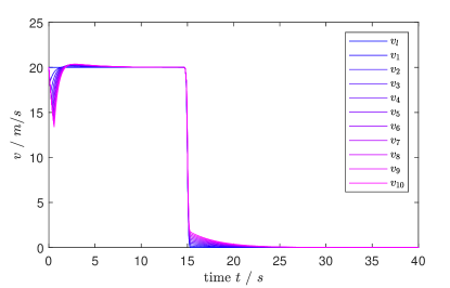
(b) Fig. 3b: Velocities

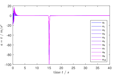
(c) Fig. 3c: Accelerations

Figure 3: Simulation, under controller (8), of system (1) with 10 vehicles following a leader in Scenario 1 and parameters as in Table 1.

The simulation of the platoon (1) under the controller (8) in this scenario is depicted in Fig. 3. It can be seen in Fig. 3a that not only the prescribed safety and maximal distances are always guaranteed, but the inter-vehicle distances actually stay nearly constant. From Figs. 3b and 3c we can observe that the velocities and accelerations of the followers only differ from those of the leader at the beginning and after the full braking, but are identical otherwise.

Scenario 2: The leader position trajectory is chosen as $x_{l}(t)=50+15t-50\cos(t/5)+\tfrac{5}{2}\sin(2t)$ so that the leader exhibits a strongly varying acceleration.

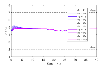
(a) Fig. 4a: Inter-vehicle distances, safety distance $d_{\min}$ and maximal distance $d_{\max}$

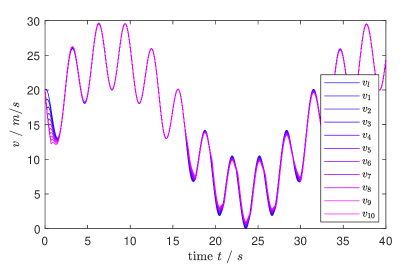
(b) Fig. 4b: Velocities

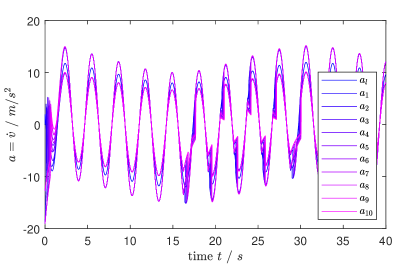
(c) Fig. 4c: Accelerations

Figure 4: Simulation, under controller (8), of system (1) with 10 vehicles following a leader in Scenario 2 and parameters as in Table 1.

The simulation of the platoon (1) under the controller (8) in this scenario is shown in Fig. 4. Again, as depicted in Fig. 4a, the inter-vehicle distances stay within the tight corridor given by the prescribed safety and maximal distances, and even remain in the middle of this corridor. The velocities and accelerations of the followers are shown in Figs. 4b and 4c and, again, they are nearly identical to that of the leader.

Overall, the simulations show that via the novel controller (8) it can be achieved that all follower vehicles in the platoon essentially have the same velocity and acceleration profiles as the leader vehicle and all inter-vehicles distances stay within a tight corridor, allowing for a very good traffic flow. All of this is guaranteed even in extreme scenarios for platoons of inhomogeneous vehicles. Furthermore, the controller can be implemented in a decentralized fashion, requiring only local information.

Although the above simulations already illustrate the various advantages of the controller (8), we like to provide an additional simulation, which better illustrates that string stability is achieved. To this end, we consider Scenario 1 with the modification that we increase the number of vehicles in the platoon to 30 and the maximal distance to $d_{\max}=22$, thus $M=20$ for the controller parameter. As initial positions we choose $x_{i}^{0}=x_{i-1}^{0}-11.5\,$\mathrm{m}$$ for $i=1,\ldots,40$. Apart from those changes, all parameters are the same as in Scenario 1. The simulation of the platoon (1) under the controller (8) for this configuration is shown in Fig. 5. It is clearly visible that the velocities reach a plateau, thus the controlled platoon exhibits practical velocity string stability. In contrast to Scenario 1, where the plateau is not established so fast, the velocities take longer to reach the equilibrium velocity again; this trade-off is to be expected.

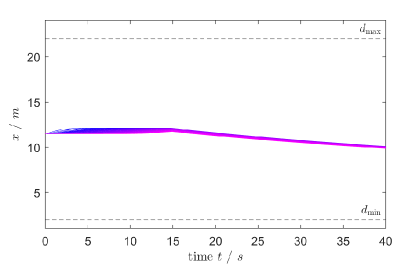
(a) Fig. 5a: Inter-vehicle distances, safety distance $d_{\min}$ and maximal distance $d_{\max}$

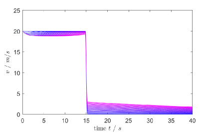
(b) Fig. 5b: Velocities

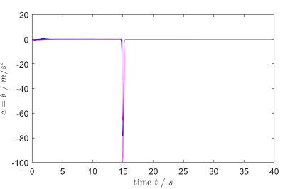
(c) Fig. 5c: Accelerations

Figure 5: Simulation, under controller (8), of system (1) with 30 vehicles following a leader in the modified Scenario 1 ($M=20$ and $x_{i}^{0}=x_{i-1}^{0}-11.5\,$\mathrm{m}$$) and parameters as in Table 1. Due to the large number of vehicles, no legend is shown. However, the color code of the vehicles follows the same rule as in Figs. 3 and 4.

5 Conclusion

We presented a new decentralized control design for vehicle platoons and have proved that it is able to both guarantee safety and a good traffic flow, and at the same time practical velocity string stability is achieved. The results were illustrated by the simulation of different scenarios. Future research should focus on the relaxation of Assumption 3.3, e.g. by allowing the vehicles to have access to some common information. Furthermore, the simulations exhibit a certain synchronization behavior of the vehicles in the platoon and it is an open question, whether this can be proved. Earlier results obtained for multi-agent systems with relative degree one [44] suggest that this is a common phenomenon. Another open question concerns the incorporation of input-constraints, which are always present in real-world applications. It should be investigated under which conditions on the parameters the control is feasible under input constraints.

References

- [1] J. K. Hedrick, M. Tomizuka, and P. Varaiya, “Control issues in automated highway systems,” IEEE Control Syst. Mag., vol. 14, no. 6, pp. 21–32, 1994.
- [2] C. Bonnet and H. Fritz, “Fuel consumption reduction in a platoon: Experimental results with two electronically coupled trucks at close spacing,” Tech. Rep., 2000, sAE International, SAE Technical Paper 2000-01-3056.
- [3] W. Levine and M. Athans, “On the optimal error regulation of a string of moving vehicles,” IEEE Trans. Autom. Control, vol. 11, pp. 355–361, 1966.
- [4] L. E. Peppard, “String stability of relative-motion pid vehicle control systems,” IEEE Trans. Autom. Control, vol. 19, no. 5, pp. 579–581, 1974.
- [5] P. Varaiya, “Smart cars on smart roads: problems of control,” IEEE Trans. Autom. Control, vol. 38, no. 2, pp. 195–207, 1993.
- [6] P. A. Ioannou and C. C. Chien, “Autonomous intelligent cruise control,” IEEE Trans. Veh. Technol., vol. 42, no. 4, pp. 657–672, 1993.
- [7] D. Swaroop and J. K. Hedrick, “Constant spacing strategies for platooning in automated highway systems,” J. Dyn. Syst. Meas. Control, vol. 121, no. 3, pp. 462–470, 1999.
- [8] A. Alam, B. Besselink, V. Turri, J. Mårtensson, and K. H. Johansson, “Heavy-duty vehicle platooning towards sustainable freight transportation: A cooperative method to enhance safety and efficiency,” IEEE Control Syst. Mag., vol. 35, no. 6, pp. 34–56, 2015.
- [9] J. Ploeg, D. P. Shukla, N. van de Wouw, and H. Nijmeijer, “Controller synthesis for string stability of vehicle platoons,” IEEE Trans. Intelligent Transp. Systems, vol. 15, no. 2, pp. 854–865, 2014.
- [10] Y. Zheng, S. E. Li, J. Wang, D. Cao, and K. Li, “Stability and scalability of homogeneous vehicular platoon: Study on the influence of information flow topologies,” IEEE Trans. Intelligent Transp. Systems, vol. 17, no. 1, pp. 14–26, 2016.
- [11] J. Guanetti, Y. Kim, and F. Borrelli, “Control of connected and automated vehicles: State of the art and future challenges,” Annual Reviews in Control, vol. 45, pp. 18–40, 2018.
- [12] T. Ersal, I. Kolmanovsky, N. Masoud, N. Ozay, J. Scruggs, R. Vasudevan, and G. Orosz, “Connected and automated road vehicles: state of the art and future challenges,” Vehicle System Dynamics, vol. 58, no. 5, pp. 672–704, 2020.
- [13] J. Lunze, Feedback Control of Large Scale Systems, ser. International Series in Systems and Control Engineering. Hemel Hempstead: Prentice-Hall, 1992.
- [14] A. A. Peters, R. H. Middleton, and O. Mason, “Leader tracking in homogeneous vehicle platoons with broadcast delays,” Automatica, vol. 50, no. 1, pp. 64–74, 2014.
- [15] P. Seiler, A. Pant, and K. Hedrick, “Disturbance propagation in vehicle strings,” IEEE Trans. Autom. Control, vol. 49, no. 10, pp. 1835–1842, 2004.
- [16] W. B. Dunbar and R. M. Murray, “Distributed receding horizon control for multi-vehicle formation stabilization,” Automatica, vol. 42, no. 4, pp. 549–558, 2006.
- [17] E. Camponogara, D. Jia, B. H. Krogh, and S. Talukdar, “Distributed model predictive control,” IEEE Control Syst. Mag., vol. 22, no. 1, pp. 44–52, 2002.
- [18] D. Swaroop and J. K. Hedrick, “String stability of interconnected systems,” IEEE Trans. Autom. Control, vol. 41, no. 3, pp. 349–357, 1994.
- [19] P. Wijnbergen and B. Besselink, “Existence of decentralized controllers for vehicle platoons: On the role of spacing policies and available measurements,” Systems & Control Letters, vol. 145, p. 104796, 2020.
- [20] G. J. L. Naus, R. P. A. Vugts, J. Ploeg, M. J. G. van de Molengraft, and M. Steinbuch, “String-stable CACC design and experimental validation: A frequency-domain approach,” IEEE Trans. Vehicular Technology, vol. 59, no. 9, pp. 4268–4279, 2010.
- [21] S. Öncü, J. Ploeg, N. van de Wouw, and H. Nijmeijer, “Cooperative adaptive cruise control: Network-aware analysis of string stability,” IEEE Trans. Intelligent Transp. Systems, vol. 15, no. 4, pp. 1527–1537, 2014.
- [22] B. Besselink and K. H. Johannson, “String stability and a delay-based spacing policy for vehicle platoons subject to disturbances,” IEEE Trans. Autom. Control, vol. 62, no. 9, pp. 4376–4391, 2017.
- [23] B. Besselink and S. Knorn, “Scalable input-to-state stability for performance analysis of large-scale networks,” IEEE Control Systems Letters, vol. 2, no. 3, pp. 507–512, 2018.
- [24] E. D. Sontag, “Smooth stabilization implies coprime factorization,” IEEE Trans. Autom. Control, vol. 34, no. 4, pp. 435–443, 1989.
- [25] S. Feng, Y. Zhang, S. E. Li, Z. Cao, H. X. Liu, and L. Li, “String stability for vehicular platoon control: Definitions and analysis methods,” Annu. Rev. Control, 2019.
- [26] A. Ilchmann, E. P. Ryan, and C. J. Sangwin, “Tracking with prescribed transient behaviour,” ESAIM Control Optim. Calc. Var., vol. 7, pp. 471–493, 2002.
- [27] T. Berger, A. Ilchmann, and E. P. Ryan, “Funnel control of nonlinear systems,” Math. Control Signals Syst., vol. 33, pp. 151–194, 2021.
- [28] C. M. Hackl, Non-identifier Based Adaptive Control in Mechatronics–Theory and Application, ser. Lecture Notes in Control and Information Sciences. Cham, Switzerland: Springer-Verlag, 2017, vol. 466.
- [29] T. Berger, S. Drücker, L. Lanza, T. Reis, and R. Seifried, “Tracking control for underactuated non-minimum phase multibody systems,” Nonlinear Dynamics, vol. 104, pp. 3671–3699, 2021.
- [30] S. Drücker, L. Lanza, T. Berger, T. Reis, and R. Seifried, “Experimental validation for the combination of funnel control with a feedforward control strategy,” Multibody System Dynamics, 2024.
- [31] T. Berger and T. Reis, “Zero dynamics and funnel control for linear electrical circuits,” J. Franklin Inst., vol. 351, no. 11, pp. 5099–5132, 2014.
- [32] A. Senfelds and A. Paugurs, “Electrical drive DC link power flow control with adaptive approach,” in Proc. 55th Int. Sci. Conf. Power Electr. Engg., 2014, pp. 30–33.
- [33] A. Pomprapa, S. Weyer, S. Leonhardt, M. Walter, and B. Misgeld, “Periodic funnel-based control for peak inspiratory pressure,” in Proc. 54th IEEE Conf. Decis. Control, 2015, pp. 5617–5622.
- [34] T. Berger, M. Puche, and F. L. Schwenninger, “Funnel control for a moving water tank,” Automatica, vol. 135, p. Article 109999, 2022.
- [35] T. Berger and A.-L. Rauert, “A universal model-free and safe adaptive cruise control mechanism,” in Proceedings of the MTNS 2018, Hong Kong, 2018, pp. 925–932.
- [36] ——, “Funnel cruise control,” Automatica, vol. 119, p. Article 109061, 2020.
- [37] C. K. Verginis, C. P. Bechlioulis, D. V. Dimarogonas, and K. J. Kyriakopoulos, “Robust distributed control protocols for large vehicular platoons with prescribed transient and steady-state performance,” IEEE Transactions on Control Systems Technology, vol. 26, no. 1, pp. 299–304, 2018.
- [38] G. Guo and D. Li, “Adaptive sliding mode control of vehicular platoons with prescribed tracking performance,” IEEE Transactions on Vehicular Technology, vol. 68, no. 8, pp. 7511–7520, 2019.
- [39] B. Armstrong-Hélouvry, P. E. Dupont, and C. Canudas-de Wit, “A survey of models, analysis tools and compensation methods for the control of machines with friction,” Automatica, vol. 30, no. 7, pp. 1083–1138, 1994.
- [40] R. I. Leine and H. Nijmeijer, Dynamics and bifurcations of non-smooth mechanical systems, ser. Lecture notes in applied and computational mechanics. Berlin-Heidelberg: Springer-Verlag, 2004, vol. 18.
- [41] A. Ilchmann, “Decentralized tracking of interconnected systems,” in Mathematical System Theory - Festschrift in Honor of Uwe Helmke on the Occasion of his Sixtieth Birthday, K. Hüper and J. Trumpf, Eds. CreateSpace, 2013, pp. 229–245.
- [42] W. Walter, Ordinary Differential Equations. New York: Springer-Verlag, 1998.
- [43] K. J. Åström and R. M. Murray, Feedback Systems: An Introduction for Scientists and Engineers. Princeton, NJ: Princeton University Press, 2008.
- [44] J. G. Lee, T. Berger, S. Trenn, and H. Shim, “Edge-wise funnel output synchronization of heterogeneous agents with relative degree one,” Automatica, vol. 156, p. Article 111204, 2023.