plain
Case Study of Novelty, Complexity, and Adaptation in a Multicellular System
Abstract
Continuing generation of novelty, complexity, and adaptation are well-established as core aspects of open-ended evolution. However, it has yet to be firmly established to what extent these phenomena are coupled and by what means they interact. In this work, we track the co-evolution of novelty, complexity, and adaptation in a case study from the DISHTINY simulation system, which is designed to study the evolution of digital multicellularity. In this case study, we describe ten qualitatively distinct multicellular morphologies, several of which exhibit asymmetrical growth and distinct life stages. We contextualize the evolutionary history of these morphologies with measurements of complexity and adaptation. Our case study suggests a loose — sometimes divergent — relationship can exist among novelty, complexity, and adaptation.
Introduction
The challenge, and promise, of open-ended evolution has animated decades of inquiry and discussion within the artificial life community (packard2019overview). The difficulty of devising models that produce continuing open-ended evolution suggests profound philosophical or scientific blind spots in our understanding of the natural processes that gave rise to contemporary organisms and ecosystems. Already, pursuit of open-ended evolution has yielded paradigm-shifting insights. For example, novelty search demonstrated how processes promoting non-adaptive diversification can ultimately yield adaptive outcomes that were previously unattainable (lehman2011abandoning). Such work lends insight to fundamental questions in evolutionary biology, such as the relevance — or irrelevance — of natural selection with respect to increases in complexity (lehman2012evolution; Lynch8597) and the origins of evolvability (lehman2013evolvability; Kirschner8420). Evolutionary algorithms devised in support of open-ended evolution models also promise to deliver tangible broader impacts for society. Possibilities include the generative design of engineering solutions, consumer products, art, video games, and AI systems (nguyen2015; stanley2017open).
Preceding decades have witnessed advances toward defining — quantitatively and philosophically — the concept of open-ended evolution (lehman2012beyond; dolson2019modes; bedau1998classification) as well as investigating causal phenomena that promote open-ended dynamics such as ecological dynamics, selection, and evolvability (dolson2019constructive; soros2014identifying; huizinga2018emergence). The concept of open-endedness is fundamentally characterized by intertwined generation of novelty, functional complexity, and adaptation (taylor2016open). How and how closely these phenomena relate to one another remains an open question. Here, we aim to complement ongoing work to develop a firmer theoretical understanding of the relationship between novelty, complexity, and adaptation by exploring the evolution of these phenomena through a case study using the DISHTINY digital multicelullarity framework (moreno2019toward) . We apply a suite of qualitative and quantitative measures to assess how these qualities can change over evolutionary time and in relation to one another.
Methods
Simulation
The DISHTINY simulation environment tracks cells occupying tiles on a toroidal grid (size by default). Cells collect a uniform inflow of continuous-valued resource. This resource can be spent in increments of to attempt asexual reproduction into any of a cell’s four adjacent cells. A cell can only be replaced if it commands less than resource. If a cell rebuffs a reproduction attempt, its resource stockpile decrements by down to a minimum of .
In order to facilitate the formation of coherent multicellular groups, the DISHTINY framework provides a mechanism for cells to form groups and detect group membership (moreno2019toward) . Groups arise through cellular reproduction. When a cell proliferates, it may choose to initiate its offspring as a member of its kin group, thereby growing it, or induce the offspring to found a new kin group. This process is similar to the growth of biological multicellular tissues, where cell offspring can be retained as members of the tissue or permanently expelled.
We incentivize group formation by providing an additional resource inflow bonus based on group size. Per-cell resource collection rate increases linearly with group size up to a cap of 12 members. Past 12 members, the decay rate of cells’ resource stockpiles begins increasing exponentially. These mechanisms select for medium-sized groups; the harsh penalization of oversize groups, in particular, prevents any single group from consuming the entire population. Groups that are too small do not receive this bonus. Groups that are too large receive a penalty. In order to ensure group turnover, we force groups to fragment into unicells after 8,192 () updates.
In previous work , we established that this framework can select for traits characteristic of multicellularity, such as cooperation, coordination, and reproductive division of labor (moreno2021exploring) . We also found more case studies of interest arose when two nested levels of group membership were tracked as opposed to a single, un-nested level of group membership (moreno2021exploring) . With nested group membership, group growth still occurs by cellular reproduction. Cells are given the choice to retain offspring within both groups, to expel offspring from both groups, or to expel offspring from the innermost group only. In addition to being given the choice to expel or retain offspring within both groups, cells are also allowed to expel offspring from the innermost group only. In this work, we allow for nested kin groups.
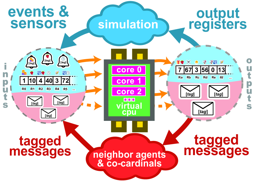
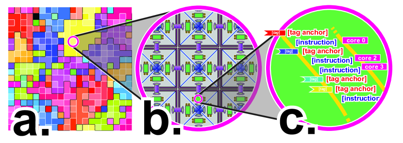
In addition to controlling reproduction behavior, evolving genomes can also share resources with adjacent cells, perform apoptosis (recovering a small amount of resource that may be shared with neighboring cells), and pass arbitrary messages to neighboring cells. Cell behaviors are controlled by event-driven genetic programs in which linear GP modules are activated in response to cues from the environment or neighboring agents; signals are handled in quasi-parallel on up to 32 virtual cores (Figure 1) (lalejini2018evolving). Each cell contains four independent virtual CPUs, all of which execute the same genetic program (Figure 2a). Each CPU manages interactions with a single neighboring cell. We refer to a CPU managing interactions with a particular neighbor as a “cardinal” (as in “cardinal direction”). These CPUs may communicate via intra-cellular message passing. Full details on the instruction set and event library used as well as simulation logic and parameter settings appear in supplementary material.
Supplementary Section E provides full detail on simulation components and parameters.
Evolution
We performed evolution in three-hour windows for compatibility with our compute cluster’s scheduling system. We refer to these windows as “stints.” We randomly generated one-hundred instruction genomes at the outset of the initial stint, stint 0. At the end of each three hour window, the system harvested and stored genomes in a population file. We then seeded subsequent stints with the previous stint’s population. No simulation state besides genome content was preserved between stints. In addition to simplifying implementation concerns, re-seeding each stint ensured that strains retained the capability to grow from a well-mixed innoculum. This facilitated later competition experiments between strains.
In order to ensure heterogeneity of biotic environmental factors experienced by evolving cells, we imposed a diversity maintenance scheme. In this scheme, descendants of a single progenitor cell from stint 0 that proliferated to constitute more than half of the population were penalized with resource loss. The severity of the penalty increased with increasing prevalence beyond half of the population. Thus, we ensured that descendants from at least two distinct stint 0 progenitors remained over the course of the simulation. We arbitrarily chose a strain for primary study — we refer to this strain as the “focal” strain and others as “background” strains. In our case study, there was only one background strain in addition to this focal strain.
In our screen for case studies, we evolved 40 independent populations for 101 stints. We selected population 16005 from among these 40 to profile as a case study due to its distinct asymmetrical group morphology.
At the conclusion of each stint, we selected the most abundant genome within the population as a representative specimen. We performed a suite of follow-up analyses on each representative specimen to characterize aspects of complexity, detailed in the following subsections. To ensure that specimens were consistently sampled from descendants of the same stint 0 progenitor, we only considered genomes with the lowest available stint 0 progenitor ID.
Phenotype-neutral Nopout
After harvesting representative specimens from each stint, we filtered out genome instructions that had no impact on the simulation.
To accomplish this, we performed sequential single-site “nopouts” where individual genome instructions were disabled by replacing them with a Nop instruction. 111 This Nop instruction was chosen to perform the same number of random number generator touches as the original instruction to control for arbitrary effects of advancing the generator. We reverted nopouts that altered a strain’s phenotype and kept those that did not. To determine whether phenotypic alteration occurred, we seeded an independent, mutation-disabled simulation with the stain in question and ran it side-by-side with an independent, mutation-disabled simulation of the wildtype strain. If any divergence in resource concentration was detected between the two strains within a 2,048 update window, the single site nopout was reverted. We continued this process until no single-site nopouts were possible without altering the genome’s phenotype. To speed up evaluation, we performed step-by-step, side-by-side comparisons using a smaller toroidal grid size of just 100 tiles.
This process left us with a “Phenoytpe-neutral Nopout” variant of the wildtype genome where all remaining instructions contributed to the phenotype.
However, in further analyses we discovered that 21 phenotype-neutral nopouts from our case study were not actually neutral — competition experiments revealed they were significantly less fit than the wildtype strain. This might be due to insufficient spatial or temporal scope to observe expression of particular genome sites in our test for phenotypic divergence.
Estimating Critical Fitness Complexity
Next, we sought to detect genome instructions that contributed to the strain fitness.
For each remaining op instruction in the Phenotype-neutral Nopout variant, we took the wildtype strain and applied a nopout at the corresponding site. We then competed this variant against the wildtype strain. Evaluating only remaining op instructions in the Phenotype-neutral Nopout variant allowed us to decrease the number of fitness competitions we had to perform.
We initialized fitness competitions by seeding a population half-and-half with two strains. We ran these competitions for 10 minutes (about 4,200 updates) on a toroidal grid, after which we assessed the relative abundances of descendants of both seeded strains.
To determine whether fitness differed significantly between a wildtype and variant strain, we compared the relative abundance of the strains observed at the end of competitions against outcomes from 20 control wildtype-vs-wildtype competitions. We fit a -distribution to the abundance outcomes observed under the control wildtype-vs-wildtype competitions and deemed outcomes that fell outside the central 98% probability density of that distribution a significant difference in fitness. This allowed us to screen for fitness effects of single-site nopouts while only performing a single competition per site.
This process left us with a “Fitness-noncritical Nopout” variant of the wildtype genome where all remaining instructions contributed to the phenotype. We called the number of remaining instructions its “critical fitness complexity.” We adjusted this figure downwards for the expected 1% rate of false-positive fitness differences among tested genome sites. This metric mirrors the MODES complexity metric described in (dolson2019modes) and the approximation of sequence complexity advanced in (adami2000evolution).
Estimating State Interface Complexity
In addition to estimating the number of genome sites that contribute to fitness, we measured the number of different environmental cues and the number of different output mechanisms that cells adaptively incorporated into behavior.
One possible way to take this measure would be to disable event cues, sensor instructions, and output registers one by one and test for changes in fitness. However, this approach would fail to distinguish context-dependent input/output from merely contingent input/output. For example, a cell might happen to depend on a sensor being set at a certain frequency but not on the actual underlying simulation information the sensor represents.
To isolate context-dependent input/output state interactions, we tested the fitness effect of swapping particular input/output states between CPUs rather than completely disabling them. That is, for example, CPU would be forced to perform the output generated by CPU or CPU would be shown the input meant for CPU . We performed this manipulation on half the population in a fitness competition for each individual component of the simulation’s introspective state (44 sensor states relating to the status of a CPU’s own cell), extrospective state (61 sensor states relating to the status of a neighboring cell), and writable state (18 output states, 10 of which control cell behavior and 8 of which act as global memory for the CPU). 222 A full description of each piece of introspective, extrospective, and writable state is listed in supplementary material. We deemed a state as fitness-critical if this manipulation resulted in decreased fitness at significance using a -test parameterized by 20 control wild-type vs wild-type competitions.
We describe the number of states that cells interact with to contribute to fitness as “State Interface Complexity.”
Estimating Messaging Interface Complexity
In addition to estimating the number of input/output states cells use to interact with the environment, we also estimated the number of distinct intra-cellular messages cardinals within a cell use to coordinate and inter-cellular messages that cells use to coordinate. As with state interface complexity, distinguishing context-dependent behavior from contingent behavior is critical to attaining a meaningful measurement. For example, a cardinal might happen to depend on always receiving a inter-cellular message from a neighbor or an intra-cellular message from another cardinal. Although meaningless, if that message were blocked, fitness would decrease. So, instead of simply discarding messages to test for a fitness effect, we re-route messages back to the sending cardinal instead of their intended recipient. We deemed a messages as fitness-critical if this manipulation resulted in decreased fitness at significance using a -test parameterized by 20 control wild-type vs wild-type competitions.
We refer to the number of distinct messages that cells send to contribute to fitness as “Messaging Interface Complexity.”
We refer to the sum of State Interface Complexity, Intra-messaging Interface Complexity, and Inter-messaging Interface Complexity as “Cardinal Interface Complexity.”
Estimating Adaptation
In order to assess ongoing changes in fitness, we performed fitness competitions between the representative focal strain specimen sampled at each stint and the focal strain population from the preceding stint. (Recall from Section Evolution that, due to a diversity maintenance procedure, two completely independent strains coexisted over the course of the experiment — the “focal” strain selected for analysis and a “background” strain.) Using the population from the preceding stint as the competitive baseline (rather than the representative specimen) ensured more focused, consistent measurement of the fitness properties of the specimen at the current stint (e.g., preventing skewed results from a sampled “dud” at the preceding stint).
We performed 20 independent replicates of each competition. Competing strains were well-mixed within the full-sized toroidal grid at the outset of each competition, which lasted for 10 minutes of wall time. This was sufficient to simulate about 8,000 updates at stint 0 and 2,000 updates at stint 100 (Supplementary Figures 23, 25, and 24). We determined that a gain of fitness had occurred if the current stint specimen constituted a population majority at the conclusion of more than 17 of those competitions, corresponding to a significance level of under the two-tailed binomial null hypothesis. Likewise, we deemed winning fewer than 3 competitions a significant fitness loss.
Implementation
We employed multithreading to speed up execution. We split the simulation into four subgrids. Each subgrid executed asynchronously, using the Conduit C++ Library to orchestrate best-effort, real-time interactions between simulation elements on different threads (moreno2021conduit) . This approach is inspired by Ackley’s notion of indefinite scalability (ackley2014indefinitely). In other work benchmarking the system, we have demonstrated that this approach improves scalability. The simulation scales to 4 threads with 80% efficiency, up to 64 threads with 40% efficiency and up to 64 nodes with 80% efficiency (moreno2021conduit) .
Over the 101 three-hour evolutionary stints performed to evolve the case study, 7,565,309 simulation updates elapsed. This translates to 74,904 updates elapsed per stint or about 6.9 updates per second. However, the update processing rate was not uniform across stints: the simulation slowed about 77% as stints progressed. Supplementary Figure 22 shows elapsed updates for each stint. During stint 0, 176,816 updates elapsed (about 16.3 updates per second). During stint 100, only 41,920 updates elapsed (about 3.8 updates per second).
Although working asynchronously, threads processed similar number of updates during each stint. The mean standard deviation of update-processing rate between threads was 2%. The mean difference of the update-processing rate between the fastest and slowest threads was 5%. The maximum value of these statistics observed during a stint was 9% and 20%, respectively, at stint 44. Supplementary Figure 22(b) shows the distribution of elapsed updates across threads for each stint evolved during the case study.
Software is available under a MIT License at https://github.com/mmore500/dishtiny. All data is available via the Open Science Framework at https://osf.io/prq49. Supplementary material is available via the Open Science Framework at https://osf.io/gekc8.
Results
Evolutionary History
Due to the parallel nature of the experimental framework, we did not perform perfect phylogeny tracking.
However, we did track the total number of ancestors seeded into stint 0 with extant descendants. At the end of stints 0 and 1, three distinct original phylogenetic roots were present in the population. From stint 2 onward, only two distinct original phylogenetic roots were present.
We performed follow-up analyses on specimens sampled from the lowest original phylogenetic root ID present in the population. 333 This approach was designed to choose an arbitrary strain as focal. Barring extinction, that same strain will then be identified as focal consistently across subsequent stints. Phylogenetic root ID had no functional consequences; it is simply an arbitrary basis for focal strain selection. For the first two stints, the focal strain was root ID 2,378. During stint 2, original phylogenetic root 2,378 went extinct. So, all further follow-up analyses were sampled from descendants of ancestor 12,634.
We also tracked the number of genomes reconstituted at the outset of each stint with extant descendants at the end of that stint. This count grows from approximately 10 around stint 15 to upwards of 30 around stint 40 (Supplementary Figure 17(a)). Among descendants of the lowest original phylogenetic root, the number of independent lineages spanning a stint also increases from around 5 to around 15 (Supplementary Figure 17(b)). This decrease in phylogenetic consolidation on a stint-by-stint basis correlates with the waning number of simulation updates performed per stint (Supplementary Figures 17(c) and 17(d)). More complete phylogenetic data will be necessary in future experiments to address questions about the possibility of long-term stable coexistence beyond the two strains supported under the explicit diversity maintenance scheme.
On the specimen from stint 100 used in the final case study, an evolutionary history of 20,212 cell generations had elapsed. Of these cellular reproductions, 11,713 (58%) had full kin group commonality, 7,174 had partial kin group commonality (35%), and 1,325 had no kin group commonality (7%). On this specimen, 1,672 mutation events had elapsed. During these events, 7,240 insertion-deletion alterations had occurred and 26,153 point mutations had occurred. This strain experienced a selection pressure of 18% over its evolutionary history, meaning that only 82% of the mutations that would be expected given the number of cellular reproductions that had elapsed were present.
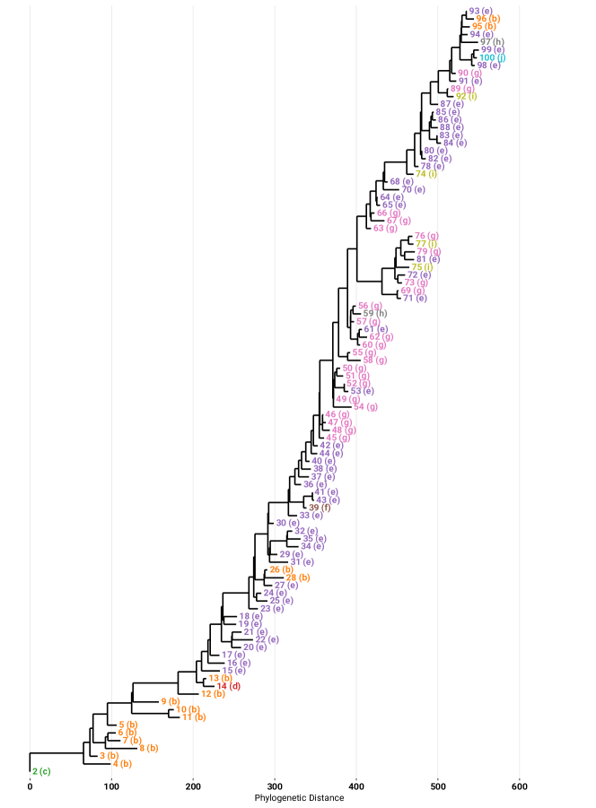
In order to characterize the evolutionary history of the experiment in greater detail, we performed a parsimony-based phylogenetic reconstruction on the sampled representative specimens from each stint, shown in Figure 3. We used genomes’ fixed-length blocks of 35 64-bit tags that mediate environmental interactions as the basis for this reconstruction. These tag blocks underwent bitwise mutation over the course of the experiment.444 In future experiments, we plan to incorporate new methodology for “hereditary stratigraph” genome annotations expressly designed to facilitate phylogenetic reconstruction (moreno2022hereditary) . Supplementary Figure 18 shows hamming distance between all pairs of tag blocks. We additionally tried several other tree inference methods, discussed in supplementary material; however, these yielded lower-quality reconstructions.
Although the phylogeny of stint representatives includes many instances that do not constitute a string lineage (i.e., each stint’s representative descending directly from the preceding stint’s representative), we did not observe evidence of long-term coexistence of clades over more than ten stints.
Qualitative Morphological Categorizations
| ID | Morphology | Snapshot | Video |
|---|---|---|---|
| \cellcolor[HTML]4C72B0 a | Individual cells, no multi-cellular kin groups. Resource use is low—most cells simply hoard resource until their stockpile is beyond sufficient to reproduce. Only a handfuls of cells intermittently expend resource. |
|
https://hopth.ru/21/b=prq49+s=16005+t=0+v=video+w=specimen |
| \cellcolor[HTML]DD8452 b | Mostly individual cells, with some two-, three-, and four-cell groups evenly spread out. Resource usage occurs in short spurts in one or two adjacent cells. |
|
https://hopth.ru/21/b=prq49+s=16005+t=1+v=video+w=specimen |
| \cellcolor[HTML]55A868 c | Large multi-cellular groups dominate, consisting of hundreds of cells. Group growth is unchecked and continues until cells’ resource stockpiles are entirely depleted by the excess group size penalty. |
|
https://hopth.ru/21/b=prq49+s=16005+t=2+v=video+w=specimen |
| \cellcolor[HTML]C44E52 d | Clear groups of 10 to 15 cells in size form. Cell proliferation appears somewhat more active at the periphery of groups compared to the interior. |
|
https://hopth.ru/21/b=prq49+s=16005+t=14+v=video+w=specimen |
| \cellcolor[HTML]8172B3 e | Groups are visibly elongated along the horizontal axis. After initial development, some gradual, irregular growth occurs along the vertical axis. |
|
https://hopth.ru/21/b=prq49+s=16005+t=15+v=video+w=specimen |
| \cellcolor[HTML]937860 f | Groups are horizontally elongated similarly to morphology , but have a greater consistent vertical thickness of three or four cells. |
|
https://hopth.ru/21/b=prq49+s=16005+t=39+v=video+w=specimen |
| \cellcolor[HTML]DA8BC3 g | Initial group growth is almost entirely horizontal, with groups usually taking up only one row of cells. However, after an apparent timing cue groups perform a brief bout of aggressive vertical growth. |
|
https://hopth.ru/21/b=prq49+s=16005+t=45+v=video+w=specimen |
| \cellcolor[HTML]8C8C8C h | Groups grow horizontally and then proliferate vertically on a timing cue like morph . However, after that timing cue cell proliferation is incessant with almost no resource retention. |
|
https://hopth.ru/21/b=prq49+s=16005+t=59+v=video+w=specimen |
| \cellcolor[HTML]CCB974 i | Irregular groups of mostly less than ten cells. Incessant proliferation with almost no resource retention leads to rapid group turnover. |
|
https://hopth.ru/21/b=prq49+s=16005+t=74+v=video+w=specimen |
| \cellcolor[HTML]64B5CD j | Groups grow horizontally and then proliferate vertically on a timing cue like morph . However, several viable horizontal-bar offspring groups form before force-fragementation. |
|
https://hopth.ru/21/b=prq49+s=16005+t=100+v=video+w=specimen |
![[Uncaptioned image]](/html/2405.07241/assets/snapshots/sanitized/a=kin-group-id+idx=0+proc=0+series=16005+stint=0+thread=0+update=28991+ext=.png)
![[Uncaptioned image]](/html/2405.07241/assets/snapshots/sanitized/a=kin-group-id+idx=0+proc=0+series=16005+stint=1+thread=0+update=14271+ext=.png)
![[Uncaptioned image]](/html/2405.07241/assets/snapshots/sanitized/a=kin-group-id+idx=0+proc=0+series=16005+stint=2+thread=0+update=17471+ext=.png)
![[Uncaptioned image]](/html/2405.07241/assets/snapshots/sanitized/a=kin-group-id+idx=0+proc=0+series=16005+stint=14+thread=0+update=16959+ext=.png)
![[Uncaptioned image]](/html/2405.07241/assets/snapshots/sanitized/a=kin-group-id+idx=0+proc=0+series=16005+stint=15+thread=0+update=16639+ext=.png)
![[Uncaptioned image]](/html/2405.07241/assets/snapshots/sanitized/a=kin-group-id+idx=0+proc=0+series=16005+stint=39+thread=0+update=10303+ext=.png)
![[Uncaptioned image]](/html/2405.07241/assets/snapshots/sanitized/a=kin-group-id+idx=0+proc=0+series=16005+stint=45+thread=0+update=12991+ext=.png)
![[Uncaptioned image]](/html/2405.07241/assets/snapshots/sanitized/a=kin-group-id+idx=0+proc=0+series=16005+stint=59+thread=0+update=11839+ext=.png)
![[Uncaptioned image]](/html/2405.07241/assets/snapshots/sanitized/a=kin-group-id+idx=0+proc=0+series=16005+stint=74+thread=0+update=12991+ext=.png)
![[Uncaptioned image]](/html/2405.07241/assets/snapshots/sanitized/a=kin-group-id+idx=0+proc=0+series=16005+stint=100+thread=0+update=8767+ext=.png)
We performed a qualitative survey of the evolved life histories along the evolutionary timeline by analyzing video recordings of monocultures representative specimens from each stint.
Table 1 summarizes the ten morphological categories we grouped specimens into. In brief, specimens from early stints largely grew as unicellular or small multicellular groups (morphs , ). Then, the specimen from stint 14 grew as larger, symmetrical groups (morph ). At stint 15, a distinct, asymmetrical horizontal bar morphology evolved (morph ). At stint 45, a delayed secondary spurt of group growth in the vertical direction arose (morph ). This morphology was sampled frequently until stint 60 when morph began to be sampled primarily again. However, morph was observed as late as stint 90.
Phylogenetic analysis (Figure 3) indicates that observations of morph at stint 53 and onward are instances of secondary loss rather than retention of trait by a separate lineage coexisting with the lineage expressing morph . Three separate reversion events from morph to morph appear likely. Interestingly, morph individuals at stints 89 and 90 appear to represent subsequent trait re-gain after reversion from morph to morph .
Table 1 provides more detailed descriptions of each qualitative morph category as well as video and a still image example of each. Supplementary Table LABEL:tab:morph_by_stint provides morph categorization for each stint as well as links to view the stint’s specimen in a video or in-browser web simulation.
Fitness
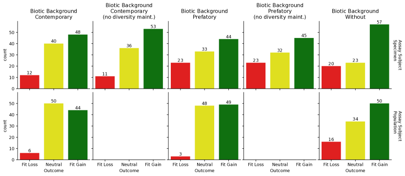
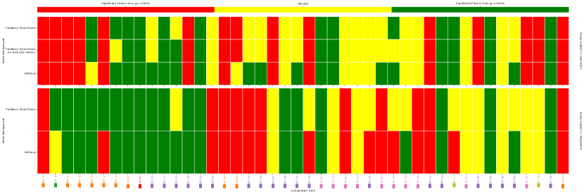
Of the 100 competition assays performed, 57 indicated significant fitness gain, 23 were neutral, and 20 indicated significant fitness loss (shown in upper right of Figure 4, at the intersection of the “Biotic Background, Without” column and “Assay Subject, Specimen” row.)
We were surprised by the frequency of deleterious outcomes, leading us to perform a second set of experiments to investigate whether these outcomes could be explained as sampling of “dud” representatives. In these competition assays, we competed the entire focal strain population against the focal strain population from the preceding stint. However, we observed a similar result: 50 assays indicated significant fitness gain, 34 were neutral, and 16 indicated significant fitness loss (shown in lower right of Figure 4, at the intersection of the “Biotic Background, Without” column and “Assay Subject, Population” row.)
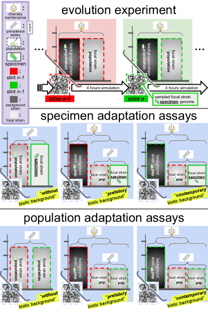
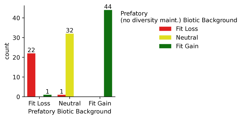
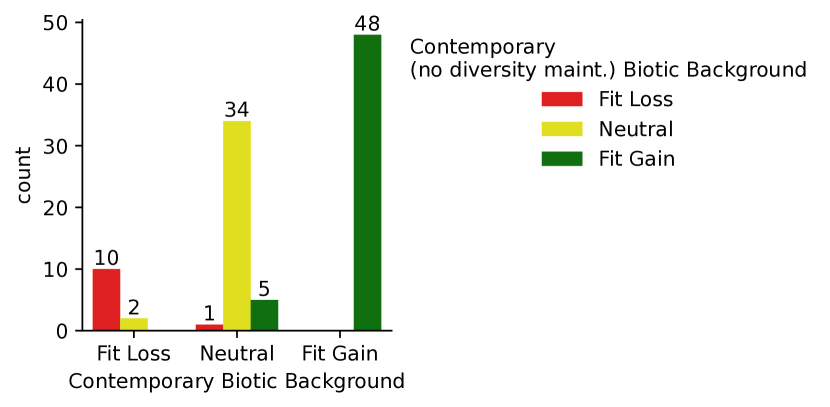
Next, we investigated whether the presence of the background strain as a “biotic background” influenced fitness. We repeated the two experiments described above (specimen and population competition assays), but inserted the background strain as half of the initial well-mixed population. In one assay setup, we used the background strain population from the current stint. We refer to this as “contemporary biotic background.” In another, which we call “prefatory biotic background,” we used the background strain population from the previous stint. We refer to the original competition assays absent the background strain as “without biotic background.” Figure 5 summarizes these competition assay designs.
tmp1\zlabelrotate\zref@extractdefaulttmp1page0
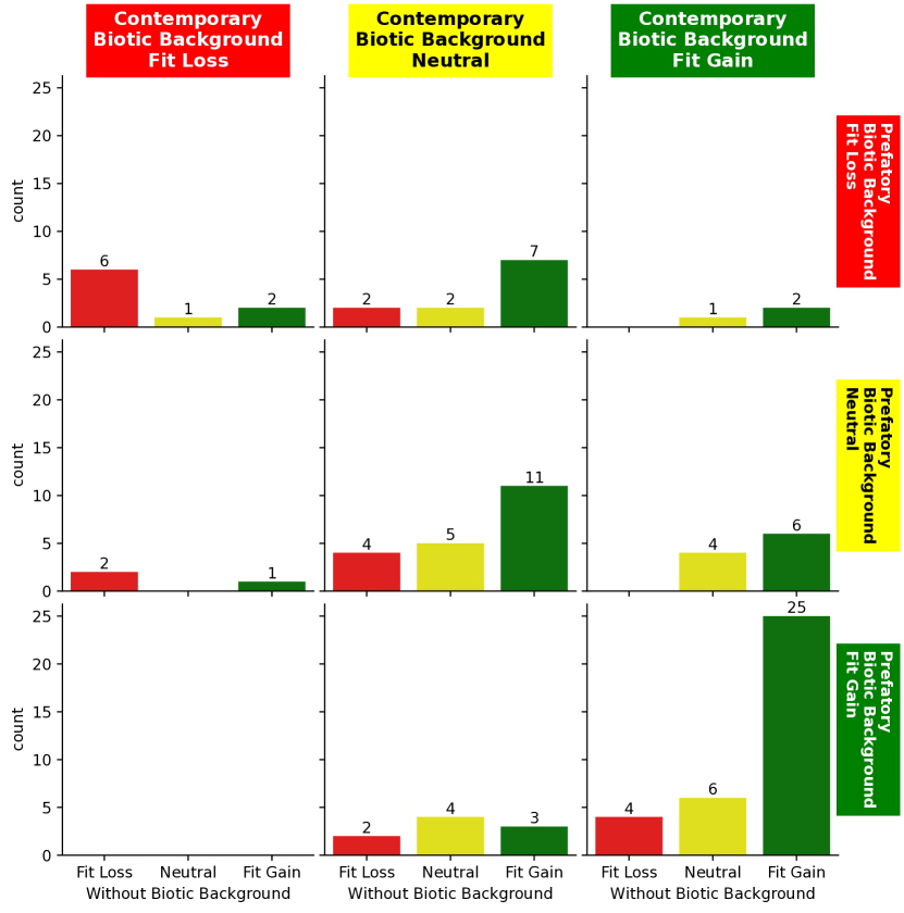
After incorporating the background strain into our measure of fitness, we detected fewer whole-population deleterious outcomes — only six under contemporary biotic background conditions and only three under prefatory biotic background conditions (Figure 4). To determine whether the presence of the background strain caused the overall reduction in whole-population deleterious outcomes, we performed a control competitions under biotic background conditions, but with the focal strain population substituted for the background strain population (Supplementary Figure 31). Under these conditions, nine of the stints where whole-population deleterious outcomes had been detected came up neutral and one, surprisingly, tested significantly adaptive (Supplementary Figure 30). Dose-dependent fitness effects and/or reduced experimental sensitivity of the biotic background assay appear to play at least a partial role in explaining the reduction of detected whole-population deleterious outcomes. However, 10 stints still tested significantly deleterious with the control focal strain biotic background in addition to without biotic background.
Four stints do provide strong, direct evidence of a selective effect by the background strain: four whole-population outcomes that were deleterious without their biotic background were actually significantly advantageous in the presence of both the prefatory and contemporary background strain populations (Figure 6(c)). All four of these stints exhibited whole-population deleterious outcomes under the control focal strain biotic background, indicating that the observed fitness sign change was specifically due to the presence of the background strain (Supplementary Figure 30).
Additionally, we detected two deleterious outcomes without biotic background as significantly adaptive under the prefatory biotic background but as neutral under contemporary biotic background (Figure 6(c)). Control focal strain biotic background experiments again suggest that the background strain, specifically, is responsible for this effect (Supplementary Figure 30).
We also found one whole-population outcome that was significantly advantageous without biotic background and in the presence of the prefatory background strain population but significantly deleterious in the presence of the contemporary background strain, possibly suggesting a “arms race”-like evolutionary innovation on the part of the background strain over that stint (Figure 6(c)).
Nonetheless, we still saw three whole-population outcomes that were significantly deleterious under all three conditions (Figure 6(c)). These whole-population outcomes were also deleterious under the control focal strain biotic background experiments (Supplementary Figure 30). Muller’s ratchet (andersson1996muller) or maladaptation due to environmental change (brady2019causes) may provide possible explanations, but a definitive answer will require further study.
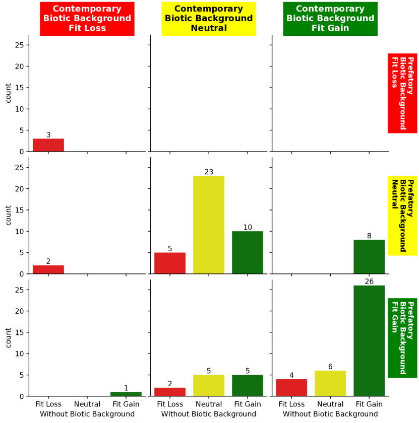
We also performed fitness assays on individual sampled specimens with both biotic backgrounds. Out of 100 stints tested, we observed 20 significantly deleterious outcomes without biotic background, 23 significantly deleterious outcomes under prefatory biotic background, and 12 significantly deleterious outcomes under contemporary biotic background (Figure 4). Unlike the whole-population deleterious outcomes discussed above, some deleterious outcomes from sampled specimens is not surprising. Evolving populations naturally contain standing variation in fitness (martin2016nonstationary), so occasional sampling of less-fit individuals should be expected. Reciprocally, we observed 57 significantly adaptive outcomes without biotic background, 44 with prefatory biotic background, and 48 with contemporary biotic background (Figure 4). Greater sensitivity of the “without biotic background” adaptation assay could account for the counterintuitive detection of more adaptive outcomes under abiotic conditions (i.e., the absence of the background strain).
As before with the population-level adaptation assays, we detected four specimen outcomes that were deleterious without biotic background but significantly advantageous under both tested background strain populations (Figure 6(a)). Additionally, and again as before, we detected two deleterious outcomes without biotic background as significantly adaptive under the prefatory biotic background but as neutral under the contemporary biotic background (Figure 6(a)). Control focal strain biotic background experiments confirm that the background strain, specifically, is responsible for these effects (Supplementary Figure 30).
We found no specimen outcomes that were advantageous under the prefatory biotic background but deleterious under the contemporary background. However, we found three stints with opposite dynamics: specimen outcomes deleterious under prefatory biotic background but advantageous under contemporary biotic background (Figure 6(a)), further suggesting coincident, interacting evolutionary innovations along focal and background strain lineages (Figure 6(a)).
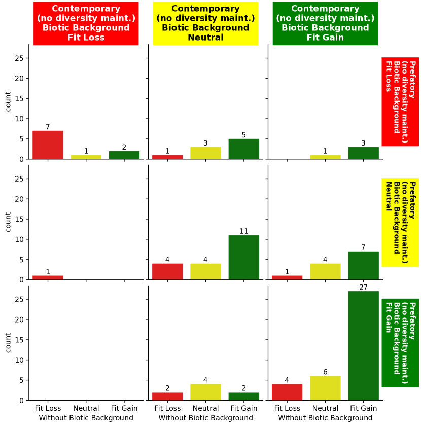
To better characterize the mechanism behind fitness effects caused by the background strain, we performed additional specimen adaptation assays under biotic background conditions with diversity maintenance disabled. This analysis allowed us to test whether action of the diversity maintenance mechanism, rather than direct interactions between the focal and background strains, caused the observed fitness effects. Figure 7 compares adaptation assay outcomes with and without diversity maintenance under both the prefatory and contemporary biotic background conditions. Outcomes were generally similar, and we observed only one sign-change difference was observed: one specimen outcome was beneficial under prefatory biotic background conditions without diversity maintenance but deleterious with diversity maintenance. Further, as shown in Figure 6(b), without diversity maintenance we still to observed four outcomes that were advantageous only under biotic conditions and instead tested deleterious under abiotic conditions. So, biotic selective effects cannot be explained as an artifact of activation of the diversity maintenance scheme.555 We also conducted specimen adaptation assays with diversity maintenance disabled under the control focal strain biotic background. In these experiments, we again found no evidence for impact from the diversity maintenance scheme on results (Supplementary Figure 30).
tmp2\zlabelrotate\zref@extractdefaulttmp2page0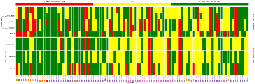
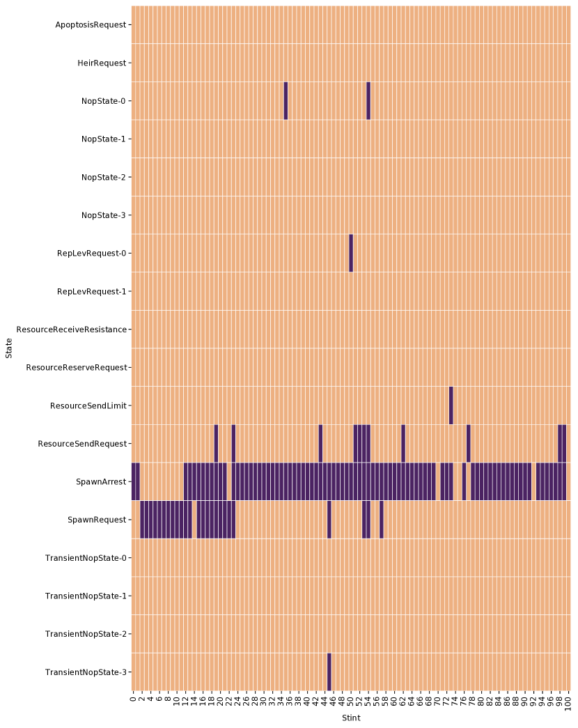
Significant increases in fitness occur throughout the evolutionary history of the case study, but not at every stint. Figure 8 summarizes the outcome of all adaptation assays stint-by-stint across evolutionary history. Neutral outcomes appear to occur more frequently at later stints. This may be indicative of slower evolutionary innovation, but may also result to some extent from simulation of fewer generations during evolutionary stints (Supplementary Figure 22) and during competition experiments (Supplementary Figure 25) due to slower execution of later genomes.
tmp3\zlabelrotate\zref@extractdefaulttmp3page0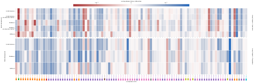
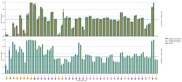
Figure 9 shows the magnitudes of calculated fitness differentials for all adaptation assays. Fitness differentials during the first 40 stints are generally higher magnitude than later fitness differentials, although a strong fitness differential occurs at stint 93. Although the emergence of morphology was associated with significant increases in fitness in some specimen assays and morphologies and were associated with significant increases in fitness across all specimen assays (Figure 8), the magnitude of these fitness differentials appears ordinary compared to fitness differentials at other stints (Figure 9). Supplementary Figure 26 shows mean end-competition prevalence across assays, telling a similar story.
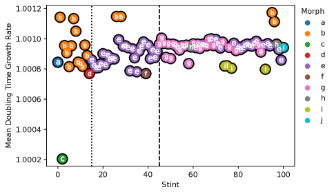
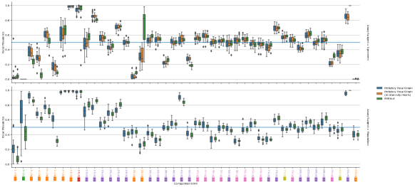
In addition to competition assays, we also measured growth rate of specimen strains by tracking doubling time (in updates) when seeded into quarter-full toroidal grids (Figure 10). Morph exhibited a fast growth rate early on that was never matched by later morphs. This measure appears to be a poor overall proxy for fitness, highlighting the importance of biotic aspects of the simulation environment which are not present in the empty space the assayed cells double into.
Fitness Complexity
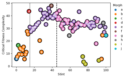
Figure 11 plots critical fitness complexity of specimens drawn from across the case study’s evolutionary history.
Critical fitness complexity reaches more than 20 under morph , jumps to more than 40 under morph , drops to slightly more than 30 for morph . Critical fitness complexity reaches a peak of 48 sites around stint 39 then levels out and decreases. This decrease may in part be due to declining sensitivity of competition experiments due to slower simulation resulting in execution of fewer updates within the fixed-duration jobs (Supplementary Figure 23).
Phylogenetic analysis (Figure 3) suggests independent origins of the critical fitness complexity in morph and morph — the morph specimen from stint 14 is more closely related to the morph specimen from stint 13 than to the morph specimen from stint 15. Likewise, specimens of lower complexity morphs and that appear past stint 70 appear to have independent evolutionary origins.
Interface Complexity
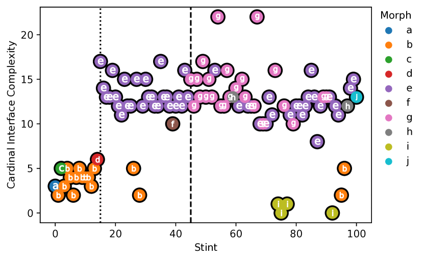
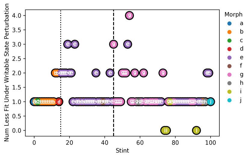
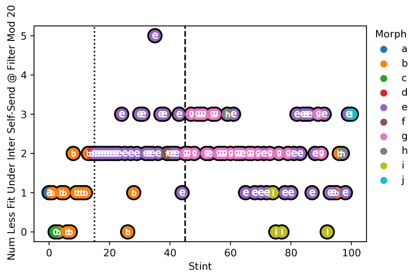
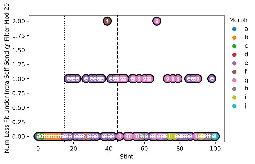
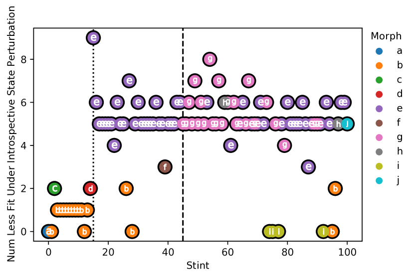
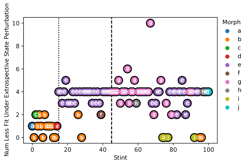
Figure 12 summarizes cardinal interface complexity, as well as its constituent components, for specimens drawn from across the case study’s evolutionary history.
Notably, cardinal interface complexity more than doubles from 6 interactions to 17 interactions coincident with the emergence of morph (Figure 12(a)). This is due to simultaneous increases in extrospective state sensing (2 to 9 states; Figure 12(f)), introspective state sensing (1 to 4 states; Figure 12(e)), and writable state usage (1 to 2 states; Figure 12(b)).
The emergence of morph coincided with an increase in writable state interface complexity from 1 to 3 as shown in Figure 12(b). However, morph was not associated with other changes in other aspects of cardinal interface complexity. The greatest observed cardinal interface complexity was 22 interactions at stints 54 and 67.
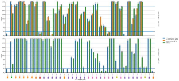
Genome Size
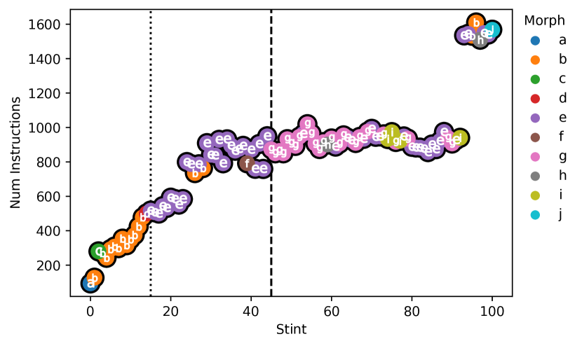
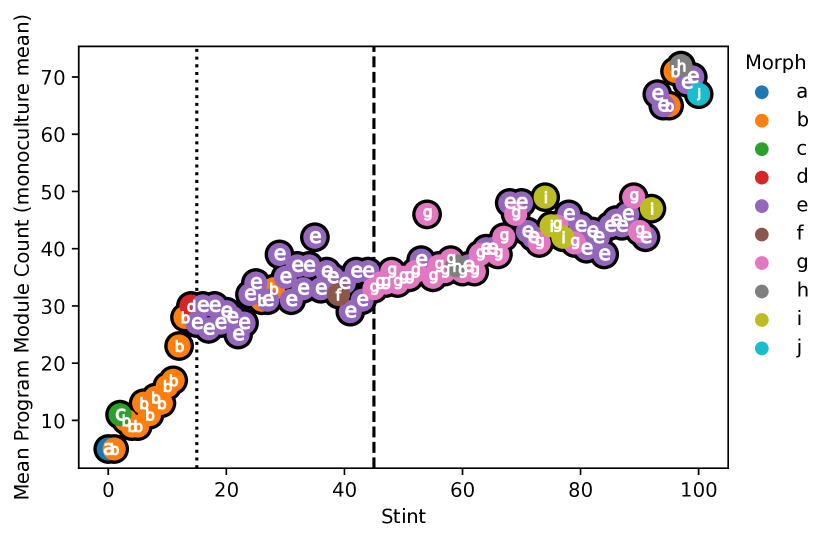
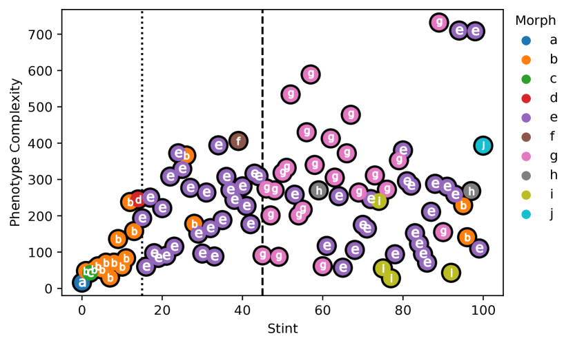
Figure 13 shows evolutionary trajectories of three genome size metrics in sampled focal strain specimens. Instruction count and module count increased from 100 and 5 to around 800 and 30, respectively, between stints 0 and 40. Within this period at stint 24, instruction count jumped from around 600 to more than 800 and module count jumped by about 5. This was coincident with detection in our adaptation assays of population-level sign-change mediation of adaptation by the background strain (Figure 8). In sampled specimen fitness assays at stint 24, we detected significant increases in fitness in the presence of the background strain but no significant change in fitness in its absence.
Between stints 40 and 90, module count gradually increased to around 40 while instruction count remained stable. Then, at stint 93, instruction count jumped to around 1,500 and module count jumped to around 60. This was coincident with the strong fitness differentials observed at stint 93 (Figure 9).
To better understand the functional effects of changes in genome size, we additionally measured the number of instructions that affected agent phenotype, shown as “phenotype complexity” in Figure 13(c). This measure can be considered akin to a count of “active” sites.
Phenotype complexity varied greatly stint to stint. The median value increased from nearly 0 to around 200 sites between stints 0 and 40. Between stints 40 and 90, we observed phenotype complexity values ranging from less than 100 to more than 500. Morph specimens appear to show particularly great variance in phenotype complexity. The first observed morph specimen at stint 45 exhibited relatively low phenotype complexity of around 100 active sties. The highest phenotype complexity values of around 700 were measured from three specimens of morphs and in the last ten stints.
Discussion
Throughout the case study lineage, we describe an evolutionary sequence of ten qualitatively distinct multicellular morphologies (Table 1). The emergence of some, but not all, of these morphologies coincided with an increase in fitness compared to the preceding population. Outcomes from the first observed morphology specimen are significantly deleterious in all contexts. Likewise, morphology , while advantageous in the absence of the background strain, appeared neutral in its presence (Figure 8). However, the genesis of morphology , and are associated with significant fitness gain in all contexts (Figure 8). This latter set of novelties might be described as “innovations,” which Hochberg et al. define as qualitative novelty associated with an increase in fitness (hochberg2017innovation). Interestingly, the magnitude of the fitness differentials associated with the emergence of morphologies , and do not appear to fall outside the bounds of other stint-to-stint fitness differentials (Figure 9).
The relationship between innovation and complexity also appears to be loosely coupled. The emergence of morphology was accompanied by a spike in critical fitness complexity (from 25 sites at stint 13 to 43 sites at stint 14). However, the emergence of morphology coincided with a loss of critical fitness complexity (from more than 30 sites to fewer than 10 sites). The specimen of morph at stint 77, which phylogenetic analysis suggests may have independent trait origin from the specimen at stint 75, exhibited significant fitness gain across all contexts despite decimation of complexity.
Phylogenetic analysis suggests that morphology was not a direct descendant of morphology . So the emergence of morphology appears to have coincided with a more modest increase in fitness complexity from 25 sites to 31 sites. Similarly, the emergence of morphology with 42 critical sites at stint 45 coincided with a relatively modest increase in fitness complexity from 39 critical sites at stint 44.
We also see evidence that increases in complexity do not imply qualitative novelty in morphology. In Figure 11, we can also observe notable increases in critical fitness complexity that did not coincide with apparent morphological innovation. For example, fitness complexity jumped from 11 sites at stint 11 to 27 sites at stint 12 while morphology was retained. In addition, a more gradual increase in fitness complexity was observed from 27 sites at stint 16 to 46 sites at stint 36 all with consistent morphology .
Finally, we also observed disjointedness between alternate measures of functional complexity. Notably, critical fitness complexity increased by 18 sites with the emergence of morph but interface complexity increased only marginally. Subsequently observed morph had nearly triple the interface complexity of morph (6 interactions vs. 17 interactions) but had 12 sites lower critical fitness complexity. In addition, the gradual increase in critical fitness complexity between stint 15 and 36 under morphology is not accompanied by a clear change in interface complexity (Figures 12(a) and 11). These apparent inconsistencies between metrics for functional complexity evidence the multidimensionality of this idea and underscore well-known difficulties in attempts to describe and quantify it (bottcher2018molecules).
Conclusion
Complexity and novelty are not inevitable outcomes of Darwinian evolution (stanley2017open). Instead, how and why some lineages within some model systems evolve complexity and novelty merits explanation.
Efforts to develop substrates and conditions sufficient to observe the evolution of complexity and novelty plays a crucial role in validating the sufficiency of theory. Additionally, subsequent availability of complexity and novelty potential within experimental substrates enables work to test and refine theory. The artificial life research community has a rich track record to these ends.
The case study reported here tracks a lineage over two phenotypic innovations and several-fold increases in complexity. DISHTINY relaxes common simulation constraints (goldsby2012task; goldsby2014evolutionary), enabling broad genetic determination of multicellular life history and allowing for unconstrained cellular interactions between multicellular bodies. As such, this case study opens new windows into evolutionary origins of complexity and novelty, especially with respect to biotic interactions.
Our case study exhibits loose coupling between novelty, complexity, and adaptation. We observe instances where novelty coincides with adaptation and instances where it does not. We observe instances where increases in complexity coincide with adaptation and where decreases in complexity coincide with adaptation. We observe instances where innovation coincides with spikes in complexity and instances where it does not. We even observe contradiction between metrics that measure different aspects functional complexity. For example, the specimen sampled at stint 15 had near triple the interface complexity of the specimen sampled at stint 14 but lower critical fitness complexity.
Loose coupling between the conceptual threads of novelty, complexity, and adaptation in this case study highlights the importance of considering these factors independently when developing open-ended evolution theory — direct coupling among them cannot be assumed.
Our observation of significant selective effects by the background strain suggests it may serve a crucial role in understanding the focal strain. Future work should characterize trajectories of adaptation, novelty, and complexity in this background strain. Additionally, success of the biotic background in fleshing out our adaptation assays suggests that complexity measures could be improved through similar incorporation of the biotic background. It would be particularly interesting to measure the contribution of the background strain to complexity as the difference between complexity statistics with and without the biotic background. To more systematically test the role of biotic selection on facilitating evolution of complexity, future experiments might test for differences in the rate of high-complexity evolutionary outcomes between evolution experiments with and without long-term coexistence between lineages (i.e., diversity maintenance mechanism enabled versus disabled).
This case study highlights the potential usefulness of toolbox-based approaches to analyzing open-ended evolution systems in which an array of analyses are performed to distinguish disparate dimensions of open-endedness (dolson2019modes). Our findings emphasize, in particular, the critical role of biotic context in such analyses. In future work, we are interested in further extending this toolbox. One priority will be estimating epistatic contributions to fitness without resorting to all-pairs knockouts or other even more extensive assays. Such methodology will be crucial for systems where fitness is implicit and expensive to measure.
Acknowledgements
Thanks to members of the DEVOLAB, in particular Katherine Perry for help implementing DISHTINY visualizations. This research was supported in part by NSF grants DEB-1655715 and DBI-0939454 as well as by Michigan State University through the computational resources provided by the Institute for Cyber-Enabled Research. This material is based upon work supported by the National Science Foundation Graduate Research Fellowship under Grant No. DGE-1424871. Any opinions, findings, and conclusions or recommendations expressed in this material are those of the author(s) and do not necessarily reflect the views of the National Science Foundation.
Supplement for “Case Study of Novelty, Complexity, and Adaptation in a Multicellular System” by Matthew Andres Moreno, Santiago Rodriguez Papa, and Charles Ofria in OEE4: The Fourth Workshop on Open-Ended Evolution
In the following sections, refers to the number of hierarchical kin group levels defined for the simulation. In this work, we use .
Appendix A Virtual CPU
Each cardinal hosts a signalgp-lite virtual CPU. Each CPU can host up to 16 active virtual cores. If additional cores are required after all 16 available are in use, the oldest active core is killed and replaced. Each virtual core contains 8 virtual float registers.
Cores execute round-robin in quasi-parallel, with up to 8 instructions being executed on a single core before execution shifts to the next active core.
Like SignalGP, the signalgp-lite system uses tag-matching to determine which modules to activate in response to incoming signals from the environment, from other agents (i.e., messages), and from internal events (i.e., execution of call and fork instructions).
In the DISHTINY simulation, each CPU hosts two independent module-lookup data structures. The first module-lookup data structure is used to activate modules in response to internally-generated signals, messages from other cardinals within the same cell, and environmental events; this module-lookup data structure contains all modules within the genetic program. The second module-lookup data structure is used to activate modules in response to messages from other cells; this module-lookup data structure contains only modules with bitstring tags that end in 0. (Hence, the subset of modules with bitstring tags that end in 1 cannot be activated by messages from other cells, so that sensitive functionality like resource sharing and apoptosis can be protected from potentially malicious exploitation.)
We also use a tag-matching system to route jump instructions executed within a module. When a module is loaded, all local anchor instructions are registered within a tag-matching data structure. The local jump instruction routes to the best-matching local anchor. If no matching local anchor is available, then no jump is performed and execution continues as if a nop instruction had elapsed.
Appendix B Tag Matching
We use 64-bit bitstring tags to label modules and jump destinations. We use a variant of Downing’s streak metric to compute tag matches (downing2015intelligence). We deterministically select the single best-matching result for a tag lookup. If there is a tie, an arbitrary result is selected. For module-lookup, the best-matching tag must have a match quality at the 80th or better percentile among match qualities of pairs of randomly generated tags. Otherwise, no module is activated. For jump-lookup, the best match must be at the 50th or better percentile. Otherwise, no jump is performed.
Appendix C Program Generation and Mutation
Initial populations were seeded with programs consisting of 128 randomly generated instructions. Program length was capped at 4096 instructions.
Mutation was applied to one in 10 reproductions where any kin group commonality was maintained and to 10 in 10 reproductions where it was not. If mutation occurred, bits in the binary representation of the genome were flipped with 0.02% probability. If mutation occurred, sequence mutations were also introduced into the program at a per-site rate of 0.1%. Half of sequence mutations were deletion events, with a number of sites deleted drawn uniformly between 0 and 8. Half of sequence mutations were insertion events, with a number of sites inserted drawn uniformly between 0 and 8. When sites were inserted, half of the time randomly-generated instructions were added and half of the time existing the preceding sequence of instructions was duplicated. With 0.1% probability a sequence mutation took on severe intensity, meaning that the number of sites inserted or deleted was drawn uniformly between 0 and program size rather than between 0 and 8.
Appendix D Cooperative Resource Collection
In order to ensure kin group structure had functional ramifications, we based part of cell resource collection on the number of contiguous kin group members. To do this, we needed an efficient distributed method to approximate kin group size.
Each cell held a 64-bit bitstring with one chosen bit fixed. We estimated group size by counting the number of distinct set bits (out of 64 available slots) that were contained within a kin group. We refer to this count of distinct set bits as a group’s “quorum count.”
At every update within each tile, the simulation system broadcasts all bits that were known to be set within that tile’s kin group. This broadcast was only sent neighboring tiles that were part of the same kin group as the broadcasting tile. Each tile tracked which neighbor it learned of each set bit from so that when tiles left the kin group their set bits could be forgotten from the bits known to be set within the kin group.
This scheme was replicated independently for each kin group level simulated. For the lowest-level kin group, a different fixed bit was chosen independently for each tile. Thus, the quorum count for these lowest-level kin groups was a function of the number of cells contained. For the highest-level kin group, each tile’s fixed bit was chosen as a deterministic function of its lowest-level kin group ID. Thus, the quorum count for these highest-level kin groups was a function of the number of lowest-level kin groups contained.
To incentivize kin group formation and maintenance, we gave each cell a 0.02 resource bonus every four updates for each non-self quorum count. This bonus saturated at the simulation-defined target quorum count. For both the lowest- and highest-level kin groups we used a target quorum count of 12. The source code controlling cooperative resource collection can be found at https://github.com/mmore500/dishtiny/blob/prq49/include/dish2/services/CollectiveHarvestingService.hpp.
In addition to this cooperative resource collection mechanism, cells enjoyed a continuous resource inflow of 0.02 units per update. The source code controlling base resource inflow can be found at https://github.com/mmore500/dishtiny/blob/master/include/dish2/services/ResourceHarvestingService.hpp.
To penalize groups that expanded beyond the simulation-defined target quorum count, we decayed held resource by a multiplicative factor of , where is the excess quorum count beyond the simulation-defined target. The source code controlling cooperative resource collection can be found at https://github.com/mmore500/dishtiny/blob/prq49/include/dish2/services/CollectiveResourceDecayService.hpp.
In addition to any decay due to group size, held resource decayed at a rate of 0.05% per update. Received resource was decayed 0.099975% upon receipt.
Appendix E Simulation Details
E.1 Events
This section enumerates simulation-managed events that were dispatched on virtual CPUs. In addition to a program, each genome contained an array of 64-bit tags — one for each event. When an event’s criteria was met in the simulation, the genome’s corresponding tag was used to dispatch a module in the program and launch a core executing that module.
All events are also exposed to the cell as a corresponding input sensor. The state of the event (0 for false, 1 for true) is stored in the sensor prior to virtual CPU execution. In fact, events are triggered based on the reading of the sensor register (not by re-reading the underlying simulation state). This means that experimental perturbations that perturb sensor input also disrupted event-handling, allowing the state interface complexity metric to measure both event-driven and sensor-based behaviors.
The source code controlling events can be found at https://github.com/mmore500/dishtiny/tree/prq49/include/dish2/events and https://github.com/mmore500/dishtiny/blob/prq49/include/dish2/services/InterpretedIntrospectiveStateRefreshService.hpp.
Always
This event is always dispatched.
Is Child Cell Of
Is this cell a daughter cell of the cardinal’s neighbor? Triggered if this cell was spawned from the cardinal’s neighbor and its cell is younger than the neighbor.
Is Child Group Of (0 thru )
Is this cell’s kin group a daughter group of the cardinal’s neighbor cell’s kin group? Triggered if a cell’s kin group ancestor ID(s) are equal to the cardinal’s neighbor’s current kin group ID(s).
Is Newborn
This event is dispatched once when a cell is first born. Triggered if cell age is less than frequency at which events are launched.
Is Parent Cell Of
Is this cardinal’s cell the parent cell of the cardinal’s neighbor? Triggered if neighbor was spawned from cell and cell age is greater than neighbor age.
Kin Group Match (0 thru )
Is this cell part of the same kin group as the cardinal’s neighbor? Triggered if a cell’s kin group ID(s) are equal to the cardinal’s neighbors’ current kin group ID(s).
Kin Group Mismatch (0 thru )
Is this cell part of a different kin group from the cardinal’s neighbor cell? Triggered if a cell’s kin group ID(s) are not equal to the cardinal’s neighbors’ current kin group ID(s).
Kin Group will Expire (0 thru )
Triggered if kin group age is greater than 80% of the kin group expiration duration. (Depending on experiment configuration, the group may be force-fragmented after expiration.)
Kin Group will not Expire (0 thru )
Triggered if kin group age is less than or equal to than 80% of the kin group expiration duration.
Neighbor Apoptosis
Triggered if the most recent cell death in the cardinal’s neighbor tile was apoptosis.
Neighbor Fragmented
Triggered if the most recent cell death in the cardinal’s neighbor tile was fragmentation.
Neighbor Is Alive
Triggered if a cardinal’s neighbor tile is occupied by a live cell.
Neighbor Is Newborn
Triggered once for each time a newborn spawns into the cardinal’s neighboring tile. Triggered if the cardinal’s neighbor’s age is less than the frequency at which events are launched.
Neighbor Is Not Alive
Triggered if the cardinal’s neighboring tile is not occupied.
Neighbor Kin Group Will Expire (0 thru )
Triggered if the cardinal’s cell neighbor’s kin group age is less than or equal to 80% of the kin group expiration duration.
Neighbor Optimum Quorum Exceeded
Triggered if the cardinal’s cell neighbor’s number of known quorum bits exceed the target quorum count.
Optimum Quorum Exceeded (0 thru )
Triggered if the cell’s number of known quorum bits exceed the target quorum count.
Optimum Quorum Not Exceeded (0 thru )
Triggered if the cell’s number of known quorum bits is less than or equal to than the target quorum count.
Parent Fragmented
Triggered if a cell’s parent died from fragmentation. That is, if the last cause of death on the current tile was fragmentation.
Phylogenetic Root Match
Does this cell descend from the same originally-generated genome as its neighbor? Triggered if a cardinal’s cell’s root ID is equal to that cardinal’s neighbor cell’s root ID.
Phylogenetic Root Mismatch
Does this cell and its neighbor descend from a different originally-generated genomes? Triggered if a cardinal’s cell’s root ID is not equal to that cardinal’s neighbor cell’s Root ID.
Poorer Than Neighbor
Does this cell have less resource stockpiled than its neighbor? Triggered if a cardinal’s cell has less resource than that cardinal’s neighbor cell.
Received Resource From
Triggered if a cardinal’s cell has received resource from that cardinal’s neighbor cell.
Richer Than Neighbor
Does this cell have more resource stockpiled than its neighbor? Triggered if a cardinal’s cell has more resource in its stockpile than that cardinal’s neighbor cell.
Stockpile Depleted
Is this cell’s stockpile empty? Triggered if a cell’s stockpile is less than twice the base harvest rate.
Stockpile Fecund
Does this cell have enough stockpiled resource to fund cellular reproduction? Triggered if a cell’s stockpile is greater than 1.0.
E.2 Operations
This section overviews the operation library made available to evolving signalgp-lite genetic programs within the simulation.
Within the program section of each genome, each instruction contained
-
•
an op code, specifying which operation should be performed;
-
•
a 64-bit bitstring, used as a tag for operations that required tag-matching or as data for some configurable operations; and
-
•
three integer arguments, specifying which registers the operation should apply to (many operations do not use all arguments).
In the operation descriptions below, we refer to register access via to the th argument as reg[arg_n]. Each core has its own eight float registers. All core registers are zeroed out at core launch.
In order to prevent bread-and-butter operations like global anchors, local anchors, and terminals from being swamped out by large instruction set size, we manually defined increased “prevalences” for some instructions. This prevalence increased the probability of the operation being selected under mutations and initial program generation. Prevalence works like increasing the number of identical copies of the operation included in the operation library. We provide the prevalence of each operation below.
See https://github.com/mmore500/dishtiny/tree/prq49/include/dish2/operations for the source code of DISHTINY-specific operations and https://github.com/mmore500/signalgp-lite/tree/b6c437f44136651aa6f4051d84bc62a86c2afbbe/include/sgpl/operations for the source code of generic operations.
Refer to Section A for details on the virtual CPU running these instructions.
Fork If
| \columncolor[HTML]C0C0C0Prevalence | 1 |
| \columncolor[HTML]C0C0C0Num Args | 1 |
If reg[arg_0] is nonzero, registers a request to activate a new core with the module best-matching the current instruction’s tag. These fork requests are only handled when the current core terminates. Each core may only register 3 fork requests.
Nop, 0 RNG Touches
| \columncolor[HTML]C0C0C0Prevalence | 1 |
| \columncolor[HTML]C0C0C0Num Args | 0 |
Performs no operation for one virtual CPU cycle.
Nop, 1 RNG Touches
| \columncolor[HTML]C0C0C0Prevalence | 1 |
| \columncolor[HTML]C0C0C0Num Args | 0 |
Performs no operation for one virtual CPU cycle, and advances the RNG engine once. (Important to nop-out operations that perform one RNG touch without causing side effects.)
Nop, 2 RNG Touches
| \columncolor[HTML]C0C0C0Prevalence | 1 |
| \columncolor[HTML]C0C0C0Num Args | 1 |
Performs no operation for one virtual CPU cycle, and advances the RNG engine twice. (Important to nop-out operations that perform two RNG touches without causing side effects.)
Terminate If
| \columncolor[HTML]C0C0C0Prevalence | 1 |
| \columncolor[HTML]C0C0C0Num Args | 1 |
Terminates current core if reg[arg_0] is nonzero.
Add
| \columncolor[HTML]C0C0C0Prevalence | 1 |
| \columncolor[HTML]C0C0C0Num Args | 3 |
Adds reg[arg_1] to reg[arg_2] and stores the result in reg[arg_0].
Divide
| \columncolor[HTML]C0C0C0Prevalence | 1 |
| \columncolor[HTML]C0C0C0Num Args | 3 |
Divides reg[arg_1] by reg[arg_2] and stores the result in reg[arg_0]. Division by zero can result in an Inf or NaN value.
Modulo
| \columncolor[HTML]C0C0C0Prevalence | 1 |
| \columncolor[HTML]C0C0C0Num Args | 3 |
Calculates the modulus of reg[arg_1] by reg[arg_2] and stores the result in reg[arg_0]. Mod by zero can result in a NaN value.
Multiply
| \columncolor[HTML]C0C0C0Prevalence | 1 |
| \columncolor[HTML]C0C0C0Num Args | 3 |
Multiplies reg[arg_1] by reg[arg_2] and stores the result in reg[arg_0].
Subtract
| \columncolor[HTML]C0C0C0Prevalence | 1 |
| \columncolor[HTML]C0C0C0Num Args | 3 |
Subtracts reg[arg_2] from reg[arg_1] and stores the result in reg[arg_0].
Bitwise And
| \columncolor[HTML]C0C0C0Prevalence | 1 |
| \columncolor[HTML]C0C0C0Num Args | 3 |
Performs a bitwise AND of reg[arg_1] and reg[arg_2] then stores the result in reg[arg_0].
Bitwise Not
| \columncolor[HTML]C0C0C0Prevalence | 1 |
| \columncolor[HTML]C0C0C0Num Args | 2 |
Computes the bitwise NOT of reg[arg_1] and stores the result in reg[arg_0].
Bitwise Or
| \columncolor[HTML]C0C0C0Prevalence | 1 |
| \columncolor[HTML]C0C0C0Num Args | 3 |
Performs a bitwise OR of reg[arg_1] and reg[arg_2] then stores the result in reg[arg_0].
Bitwise Shift
| \columncolor[HTML]C0C0C0Prevalence | 1 |
| \columncolor[HTML]C0C0C0Num Args | 3 |
Shifts the bits of reg[arg_1] by reg[arg_2] positions. (If reg[arg_2] is negative, this is a right shift. Otherwise it is a left shift.) Stores the result in reg[arg_0].
Bitwise Xor
| \columncolor[HTML]C0C0C0Prevalence | 1 |
| \columncolor[HTML]C0C0C0Num Args | 3 |
Performs a bitwise XOR of reg[arg_1] and reg[arg_2] then stores the result in reg[arg_0].
Count Ones
| \columncolor[HTML]C0C0C0Prevalence | 1 |
| \columncolor[HTML]C0C0C0Num Args | 2 |
Counts the number of bits set in reg[arg_1] and stores the result in reg[arg_0].
Random Fill
| \columncolor[HTML]C0C0C0Prevalence | 1 |
| \columncolor[HTML]C0C0C0Num Args | 1 |
Fills register pointed to by reg[arg_0] with random bits chosen from a uniform distribution.
Equal
| \columncolor[HTML]C0C0C0Prevalence | 1 |
| \columncolor[HTML]C0C0C0Num Args | 3 |
Checks whether reg[arg_1] is equal to reg[arg_2] and stores the result in reg[arg_0].
Greater Than
| \columncolor[HTML]C0C0C0Prevalence | 1 |
| \columncolor[HTML]C0C0C0Num Args | 3 |
Checks whether reg[arg_1] is greater than reg[arg_2] and stores the result in reg[arg_0].
Less Than
| \columncolor[HTML]C0C0C0Prevalence | 1 |
| \columncolor[HTML]C0C0C0Num Args | 3 |
Checks whether reg[arg_1] is less than reg[arg_2] and stores the result in reg[arg_0].
Logical And
| \columncolor[HTML]C0C0C0Prevalence | 1 |
| \columncolor[HTML]C0C0C0Num Args | 3 |
Performs a logical AND of reg[arg_1] and reg[arg_2], storing the result in reg[arg_0].
Logical Or
| \columncolor[HTML]C0C0C0Prevalence | 1 |
| \columncolor[HTML]C0C0C0Num Args | 3 |
Performs a logical OR of reg[arg_1] and reg[arg_2], storing the result in reg[arg_0].
Not Equal
| \columncolor[HTML]C0C0C0Prevalence | 1 |
| \columncolor[HTML]C0C0C0Num Args | 3 |
Checks whether reg[arg_1] is not equal to reg[arg_2] and stores the result in reg[arg_0].
Global Anchor
| \columncolor[HTML]C0C0C0Prevalence | 15 |
| \columncolor[HTML]C0C0C0Num Args | 0 |
Marks a module-begin position. Based on tag-lookup, new cores or global jump instructions may set the program counter to this instruction’s program position.
This instruction can also mark a module-end position — executing this instruction can terminate the executing core. If no local anchor instruction is present between the current global anchor instruction and the preceding global anchor instruction, this operation will not terminate the executing core. (This way, several global anchors may lead into the same module.)
However, if a local anchor instruction is present between the current global anchor instruction and the preceding global anchor instruction, this operation will terminate the executing core. Local jump instructions will only consider local anchors between the preceding global anchor and the subsequent global anchor instruction.
Global Jump If
| \columncolor[HTML]C0C0C0Prevalence | 1 |
| \columncolor[HTML]C0C0C0Num Args | 2 |
Jumps the current core to a global anchor that matches the instruction tag if reg[arg_0] is nonzero. If reg[arg_1] is nonzero, resets registers.
Global Jump If Not
| \columncolor[HTML]C0C0C0Prevalence | 1 |
| \columncolor[HTML]C0C0C0Num Args | 2 |
Jumps the current core to a global anchor that matches the instruction tag if reg[arg_0] is nonzero. If reg[arg_1] is zero, resets registers.
Protected Regulator Adjust
| \columncolor[HTML]C0C0C0Prevalence | 1 |
| \columncolor[HTML]C0C0C0Num Args | 1 |
Adjusts the regulator value of global jump table tags matching this instruction’s tag by the amount reg[arg_0].
This regulator value affects the outcome of tag lookup for internal events and signals from the environment. (Note, as described in A, that independent tag lookup tables handle activating genome modules across different contexts.)
Protected Regulator Decay
| \columncolor[HTML]C0C0C0Prevalence | 1 |
| \columncolor[HTML]C0C0C0Num Args | 1 |
Ages the regulator decay countdown of global jump table tags matching this instruction’s tag by the amount reg[arg_0]. If reg[arg_0] is negative, this can forestall decay.
This decay countdown affects the outcome of tag lookup for internal events, and signals from the environment. (Note, as described in A, that independent tag lookup tables handle activating genome modules across different contexts.)
Protected Regulator Get
| \columncolor[HTML]C0C0C0Prevalence | 1 |
| \columncolor[HTML]C0C0C0Num Args | 1 |
Gets the regulator value of the global jump table tag that best matches this instruction’s tag. Stores the value in reg[arg_0].
If no tag matches, a no-op is performed.
The regulator value gotten controls internal events and signals from the environment. (Note, as described in A, that independent tag lookup tables handle activating genome modules across different contexts.)
Protected Regulator Set
| \columncolor[HTML]C0C0C0Prevalence | 1 |
| \columncolor[HTML]C0C0C0Num Args | 1 |
Sets the regulator value of global jump table tags matching this instruction’s tag to reg[arg_0].
This regulator value affects the outcome of tag lookup for internal events and signals from the environment. (Note, as described in A, that independent tag lookup tables handle activating genome modules across different contexts.)
Local Anchor
| \columncolor[HTML]C0C0C0Prevalence | 20 |
| \columncolor[HTML]C0C0C0Num Args | 0 |
Marks a program location local jump instructions may route to. This program location is tagged with the instruction’s tag.
As described in Section E.2, this operation also plays a role in determining whether global anchor instructions close a module.
Local Jump If
| \columncolor[HTML]C0C0C0Prevalence | 1 |
| \columncolor[HTML]C0C0C0Num Args | 1 |
Jumps to a local anchor that matches the instruction tag if reg[arg_0] is nonzero.
Local Jump If Not
| \columncolor[HTML]C0C0C0Prevalence | 1 |
| \columncolor[HTML]C0C0C0Num Args | 1 |
Jumps to a local anchor that matches the instruction tag if reg[arg_0] is zero.
Local Regulator Adjust
| \columncolor[HTML]C0C0C0Prevalence | 1 |
| \columncolor[HTML]C0C0C0Num Args | 1 |
Adjusts the regulator value of local jump table tags matching this instruction’s tag by the amount reg[arg_0].
Local Regulator Decay
| \columncolor[HTML]C0C0C0Prevalence | 1 |
| \columncolor[HTML]C0C0C0Num Args | 1 |
Ages the regulator decay countdown of local jump table tags matching this instruction’s tag by the amount reg[arg_0]. If reg[arg_0] is negative, this can forestall decay.
Local Regulator Get
| \columncolor[HTML]C0C0C0Prevalence | 1 |
| \columncolor[HTML]C0C0C0Num Args | 1 |
Gets the regulator value of the local jump table tag that best matches this instruction’s tag. Stores the value in reg[arg_0].
If no tag matches, a no-op is performed.
Local Regulator Set
| \columncolor[HTML]C0C0C0Prevalence | 1 |
| \columncolor[HTML]C0C0C0Num Args | 1 |
Sets the regulator value of global jump table tags matching this instruction’s tag to reg[arg_0].
Decrement
| \columncolor[HTML]C0C0C0Prevalence | 1 |
| \columncolor[HTML]C0C0C0Num Args | 1 |
Takes reg[arg_0], decrements it by one, and stores the result in reg[arg_0].
Increment
| \columncolor[HTML]C0C0C0Prevalence | 1 |
| \columncolor[HTML]C0C0C0Num Args | 1 |
Takes reg[arg_0], increments it by one, and stores the result in reg[arg_0].
Negate
| \columncolor[HTML]C0C0C0Prevalence | 1 |
| \columncolor[HTML]C0C0C0Num Args | 1 |
Negates reg[arg_0] and stores the result in reg[arg_0].
Not
| \columncolor[HTML]C0C0C0Prevalence | 1 |
| \columncolor[HTML]C0C0C0Num Args | 1 |
Performs a logical not on reg[arg_0] and stores the result in reg[arg_0].
Random Bool
| \columncolor[HTML]C0C0C0Prevalence | 1 |
| \columncolor[HTML]C0C0C0Num Args | 1 |
Stores 1.0f to reg[arg_0] with probability determined by this instruction’s tag. Otherwise, stores 0.0f to reg[arg_0].
Random Draw
| \columncolor[HTML]C0C0C0Prevalence | 1 |
| \columncolor[HTML]C0C0C0Num Args | 1 |
Stores a randomly drawn float value to reg[arg_0].
Terminal
| \columncolor[HTML]C0C0C0Prevalence | 50 |
| \columncolor[HTML]C0C0C0Num Args | 1 |
Stores a genetically-encoded value to reg[arg_0]. This value is determined deterministically using the instruction’s tag.
Exposed Regulator Adjust
| \columncolor[HTML]C0C0C0Prevalence | 1 |
| \columncolor[HTML]C0C0C0Num Args | 1 |
Adjusts the regulator value of global jump table tags matching this instruction’s tag by the amount reg[arg_0].
This regulator value affects the outcome of tag lookup for messages from neighbor cells. (Note, as described in A, that independent tag lookup tables handle activating genome modules across different contexts.)
Exposed Regulator Decay
| \columncolor[HTML]C0C0C0Prevalence | 1 |
| \columncolor[HTML]C0C0C0Num Args | 1 |
Ages the regulator decay countdown of global jump table tags matching this instruction’s tag by the amount reg[arg_0]. If reg[arg_0] is negative, this can forestall decay.
This decay countdown affects the outcome of tag lookup for messages from neighbor cells. (Note, as described in A, that independent tag lookup tables handle activating genome modules across different contexts.)
Exposed Regulator Get
| \columncolor[HTML]C0C0C0Prevalence | 1 |
| \columncolor[HTML]C0C0C0Num Args | 1 |
Gets the regulator value of the global jump table tag that best matches this instruction’s tag. Stores the value in arg[0].
If no tag matches, a no-op is performed.
The regulator value gotten controls messages from other cells. (Note, as described in A, that independent tag lookup tables handle activating genome modules across different contexts.)
Exposed Regulator Set
| \columncolor[HTML]C0C0C0Prevalence | 1 |
| \columncolor[HTML]C0C0C0Num Args | 1 |
Sets the regulator value of global jump table tags matching this instruction’s tag to reg[arg_0].
This regulator value affects the outcome of tag lookup for messages from other cells. (Note, as described in A, that independent tag lookup tables handle activating genome modules across different contexts.)
Add to Own State
| \columncolor[HTML]C0C0C0Prevalence | 5 |
| \columncolor[HTML]C0C0C0Num Args | 1 |
Adds reg[arg_0] to the current value in a target writable state then stores the sum back in to that target writable state.
To determine the target writable state, interprets the first 32 bits of the instruction tag as an unsigned integer then calculates the remainder of integer division by the number of writable states.
Broadcast Intra Message If
| \columncolor[HTML]C0C0C0Prevalence | 1 |
| \columncolor[HTML]C0C0C0Num Args | 1 |
If reg[arg_0] is nonzero, generates a message tagged with the instruction’s tag that contains the core’s current register state. Broadcasts this message to every other cardinal within the cell.
Multiply Own State
| \columncolor[HTML]C0C0C0Prevalence | 5 |
| \columncolor[HTML]C0C0C0Num Args | 1 |
Multiplies reg[arg_0] by the current value in a target writable state then stores the result back in to that target writable state.
To determine the target writable state, interprets the first 32 bits of the instruction tag as an unsigned integer then calculates the remainder of integer division by the number of writable states.
Read Neighbor State
| \columncolor[HTML]C0C0C0Prevalence | 10 |
| \columncolor[HTML]C0C0C0Num Args | 1 |
Reads a target readable state from the neighboring cell and stores it into reg[arg_0].
To determine the target readable state, interprets the first 32 bits of the instruction tag as an unsigned integer then calculates the remainder of integer division by the number of readable states.
Read Own State
| \columncolor[HTML]C0C0C0Prevalence | 20 |
| \columncolor[HTML]C0C0C0Num Args | 1 |
Reads a target readable state and stores it into reg[arg_0].
To determine the target readable state, interprets the first 32 bits of the instruction tag as an unsigned integer then calculates the remainder of integer division by the number of readable states.
Send Inter Message If
| \columncolor[HTML]C0C0C0Prevalence | 5 |
| \columncolor[HTML]C0C0C0Num Args | 1 |
If reg[arg_0] is nonzero, generates a message tagged with the instruction’s tag that contains the core’s current register state. Sends this message to the neighboring cell.
Send Intra Message If
| \columncolor[HTML]C0C0C0Prevalence | 5 |
| \columncolor[HTML]C0C0C0Num Args | 1 |
If reg[arg_0] is nonzero, generates a message tagged with the instruction’s tag that contains the core’s current register state. Sends this message to a target cardinal within the cell.
To determine the target cardinal, sums instruction arguments then calculates the remainder of integer division by the number of co-cardinals.
Write Own State If
| \columncolor[HTML]C0C0C0Prevalence | 5 |
| \columncolor[HTML]C0C0C0Num Args | 2 |
If reg[arg_1] is nonzero, stores reg[arg_0] into a target writable state.
To determine the target writable state, interprets the first 32 bits of the instruction tag as an unsigned integer then calculates the remainder of integer division by the number of writable states.
E.3 Introspective State
Introspective state refers to the collection of simulation-generated sensor values that evolving programs running within each cardinal can access via read-only operations. Each cardinal has an independent copy of each piece of introspective state state. (However, some introspective states representing cell state are set to identical values across cardinals within the same cell.)
Each cardinal’s introspective state regularly copied and dispatched to that cardinal’s neighbor cell, where it serves as read-only extrospective state.
Introspective state is organized into two categories:
-
1.
raw introspective state, and
-
2.
interpreted introspective state.
Raw introspective state directly exposes aspects of simulation state. Interpreted introspective state is filled with truthy values that are interpreted as booleans to dispatch environmentally-managed events.
See https://github.com/mmore500/dishtiny/tree/prq49/include/dish2/peripheral/readable_state/introspective_state for source code implementing introspective state.
Is Child Cell Of
| \columncolor[HTML]C0C0C0Type | char (w/ boolean semantics) |
| \columncolor[HTML]C0C0C0Category | interpreted |
Did this cell spawn from this cardinal’s neighbor cell?
Is Child Group Of (0 thru )
| \columncolor[HTML]C0C0C0Type | char (w/ boolean semantics) |
| \columncolor[HTML]C0C0C0Category | interpreted |
Does this cell’s kin group ID descend directly from the neighbor’s kin group ID?
Is Newborn
| \columncolor[HTML]C0C0C0Type | char (w/ boolean semantics) |
| \columncolor[HTML]C0C0C0Category | interpreted |
Is this cell’s age less than EVENT_LAUNCHING_SERVICE_FREQUENCY?
Is Parent Cell Of
| \columncolor[HTML]C0C0C0Type | char (w/ boolean semantics) |
| \columncolor[HTML]C0C0C0Category | interpreted |
Did this cardinal’s neighbor cell spawn from this cell? That is, was neighbor was spawned from this cell and is this cell older than neighbor?
Is Parent Group Of
| \columncolor[HTML]C0C0C0Type | char (w/ boolean semantics) |
| \columncolor[HTML]C0C0C0Category | interpreted |
Did this cell’s kin group descend directly from the cardinal’s neighbor cell’s kin group? That is, is cell’s kin group ancestor ID(s) equal to the cardinal’s neighbor’s current kin group ID(s).
Kin Group Match (0 thru )
| \columncolor[HTML]C0C0C0Type | char (w/ boolean semantics) |
| \columncolor[HTML]C0C0C0Category | interpreted |
Does this cell’s kin group ID match the neighbor’s kin group ID?
Kin Group will Expire (0 thru )
| \columncolor[HTML]C0C0C0Type | char (w/ boolean semantics) |
| \columncolor[HTML]C0C0C0Category | interpreted |
Is this cell’s kin group age greater than 80% of this level’s GROUP_EXPIRATION_DURATIONS?
Neighbor Apoptosis
Was the neighbor tile’s most recent death apoptosis?
| \columncolor[HTML]C0C0C0Type | char (w/ boolean semantics) |
| \columncolor[HTML]C0C0C0Category | interpreted |
Neighbor Fragmented
Was group fragmentation the most recent cause of death in the cardinal’s neighbor cell?
| \columncolor[HTML]C0C0C0Type | char (w/ boolean semantics) |
| \columncolor[HTML]C0C0C0Category | interpreted |
Neighbor Is Newborn
| \columncolor[HTML]C0C0C0Type | char (w/ boolean semantics) |
| \columncolor[HTML]C0C0C0Category | interpreted |
Is the neighbor’s cell age less than EVENT_LAUNCHING_SERVICE_FREQUENCY?
Neighbor Kin Group Will Expire (0 thru )
interpreted
| \columncolor[HTML]C0C0C0Type | char (w/ boolean semantics) |
| \columncolor[HTML]C0C0C0Category | interpreted |
Is this cell’s kin group age greater than 80% of the this level’s GROUP_EXPIRATION_DURATIONS?
Neighbor Optimum Quorum Exceeded (0 thru )
| \columncolor[HTML]C0C0C0Type | char (w/ boolean semantics) |
| \columncolor[HTML]C0C0C0Category | interpreted |
Is this cardinal’s neighbor cell’s kin group quorum count more than the simulation-defined target count OPTIMAL_QUORUM_COUNT?
Optimum Quorum Exceeded (0 thru )
| \columncolor[HTML]C0C0C0Type | char (w/ boolean semantics) |
| \columncolor[HTML]C0C0C0Category | interpreted |
Is this cell’s kin group quorum count more than the simulation-defined target count OPTIMAL_QUORUM_COUNT?
Parent Fragmented
| \columncolor[HTML]C0C0C0Type | char (w/ boolean semantics) |
| \columncolor[HTML]C0C0C0Category | interpreted |
Did the cell’s parent die from fragmentation? That is, was the last cause of death on the current tile was fragmentation?
Phylogenetic Root Match
| \columncolor[HTML]C0C0C0Type | char (w/ boolean semantics) |
| \columncolor[HTML]C0C0C0Category | interpreted |
Does this cell’s root ID equal the cardinal’s cell neighbor’s root ID? (This means they originate from the same seed ancestor.)
Richer Than Neighbor
| \columncolor[HTML]C0C0C0Type | char (w/ boolean semantics) |
| \columncolor[HTML]C0C0C0Category | interpreted |
Does this cell’s stockpile more resource than the cardinal’s cell neighbor?
Stockpile Depleted
| \columncolor[HTML]C0C0C0Type | char (w/ boolean semantics) |
| \columncolor[HTML]C0C0C0Category | interpreted |
Is this cell’s stockpile less than twice the base harvest rate?
Stockpile Fecund
| \columncolor[HTML]C0C0C0Type | char (w/ boolean semantics) |
| \columncolor[HTML]C0C0C0Category | interpreted |
Does this cell have enough resource stockpiled to fund spawning an offspring cell?
Cell Age
| \columncolor[HTML]C0C0C0Type | size_t |
| \columncolor[HTML]C0C0C0Category | raw |
Number CellAgeService calls elapsed since cell was born.
Epoch
| \columncolor[HTML]C0C0C0Type | size_t |
| \columncolor[HTML]C0C0C0Category | raw |
Updates elapsed since start of simulation.
Incoming Inter Message Counter
| \columncolor[HTML]C0C0C0Type | size_t |
| \columncolor[HTML]C0C0C0Category | raw |
Counter tracking incoming messages from cardinal’s neighbor cell. Intermittently reset to zero.
Incoming Intra Message Counter
| \columncolor[HTML]C0C0C0Type | size_t |
| \columncolor[HTML]C0C0C0Category | raw |
Counter of incoming messages from other cardinals within the cell. Intermittently reset to zero.
Is Alive
| \columncolor[HTML]C0C0C0Type | char (w/ boolean semantics) |
| \columncolor[HTML]C0C0C0Category | raw |
Whether the cell is alive. Although trivial as introspective state, this state is useful for neighbor cell’s extrospective state.
Kin Group Age ( thru )
| \columncolor[HTML]C0C0C0Type | size_t |
| \columncolor[HTML]C0C0C0Category | raw |
Number of epochs elapsed since kin group formation.
Kin Group ID Ancestor View ( thru )
| \columncolor[HTML]C0C0C0Type | size_t |
| \columncolor[HTML]C0C0C0Category | raw |
Kin group ID from which cell’s kin group ID is descended.
Kin Group ID View ( thru )
| \columncolor[HTML]C0C0C0Type | size_t |
| \columncolor[HTML]C0C0C0Category | raw |
Kin group ID of this cell.
Most Recent Cause of Death
raw
| \columncolor[HTML]C0C0C0Type | char |
| \columncolor[HTML]C0C0C0Category | raw |
What was this the most recent cause of death on this tile? Encoded using the CauseOfDeath enum.
Num Known Quorum Bits (0 thru )
| \columncolor[HTML]C0C0C0Type | size_t |
| \columncolor[HTML]C0C0C0Category | raw |
What is this cell’s known quorum count? (How many unique quorum bits collected from kin group members are known?)
Phylogenetic Root View
| \columncolor[HTML]C0C0C0Type | size_t |
| \columncolor[HTML]C0C0C0Category | raw |
What is this cell’s phylogenetic root ID?
(Which initially-generated ancestor is this cell descended from?)
Received Resource From
| \columncolor[HTML]C0C0C0Type | float |
| \columncolor[HTML]C0C0C0Category | raw |
How much resource is being received from the cardinal’s cell neighbor?
Resource Stockpile
| \columncolor[HTML]C0C0C0Type | float |
| \columncolor[HTML]C0C0C0Category | raw |
Amount of resource this cell has.
Spawn Count
| \columncolor[HTML]C0C0C0Type | float |
| \columncolor[HTML]C0C0C0Category | raw |
Number of offspring generated from this cell and sent to the cardinal’s neighbor tile. Includes offspring that do not successfully take into the neighbor tile or have not survived.
Spawned From
| \columncolor[HTML]C0C0C0Type | char (w/ boolean semantics) |
| \columncolor[HTML]C0C0C0Category | raw |
Did this cell spawn from this cardinal’s neighbor cell?
E.4 Writable State
Writable state refers to the collection of output values that evolving programs running within each cardinal can write to and read from. Some of these outputs enable interaction with the simulation (i.e., control phenotypic characteristics). Each cardinal has an independent copy of each piece of writable state state.
See https://github.com/mmore500/dishtiny/tree/prq49/include/dish2/peripheral/readable_state/writable_state for source code implementing writable state.
Nop State ()
| \columncolor[HTML]C0C0C0Type | float |
Writing to this state has no external effect. It can be used as global memory shared between cores.
Transient Nop State ()
| \columncolor[HTML]C0C0C0Type | float |
Writing to this state has no external effect. It is cleared regularly by the decay to baseline service. It can be used as temporary global memory shared between cores.
Apoptosis Request
| \columncolor[HTML]C0C0C0Type | char |
Writing a nonzero value to this state causes cell death.
Heir Request
| \columncolor[HTML]C0C0C0Type | char |
If this state is set when cell death occurs, the cardinal’s neighbor cell will inherit leftover resource from the cell’s stockpile.
RepLev Request (0 thru )
| \columncolor[HTML]C0C0C0Type | char |
Controls kin group inheritance for daughter cells spawned to this cardinal’s neighbor tile.
If no copies of this state are set at cell spawn, the daughter cell will have no common kin group IDs. If one copy of this state is set at cell spawn, the daughter cell will have one common kin group ID. If copies of this state are set at cell spawn, the daughter cell will have common kin group IDs.
Resource Receive Resistance
| \columncolor[HTML]C0C0C0Type | float |
Setting this state reduces the amount of resource received from the cardinal’s neighbor cell.
Resource Reserve Request
| \columncolor[HTML]C0C0C0Type | float |
Setting this state prevents that amount of stockpiled resource from being drawn from to be sent to the cardinal’s neighbor cell.
Resource Send Limit
| \columncolor[HTML]C0C0C0Type | float |
Setting this state caps the amount of resource that this cell can send to the cardinal’s neighbor cell per update.
Resource Send Request
| \columncolor[HTML]C0C0C0Type | float |
Setting this state initiates resource sharing to the cardinal’s neighbor cell. The value stored controls the amount of resource shared.
Spawn Arrest
| \columncolor[HTML]C0C0C0Type | char |
Setting this state prevents this cell from spawning offspring into this cardinal’s neighbor tile, even if sufficient resource is available.
Spawn Request
| \columncolor[HTML]C0C0C0Type | char |
Setting this state attempts to initiate spawning offspring into this cardinal’s neighbor tile.
E.5 Cellular Simulation Services
Simulation logic is applied to each cell through a collection of distinct functors, referred to as services.
All services specified to run on a particular update are applied in sequence to a single cell. (Some services run only every th update.) Then, to another randomly-chosen cell in a thread_local population, and another until the entire population has been updated.
See https://github.com/mmore500/dishtiny/tree/prq49/include/dish2/services for source code implementing these services.
Decay to Baseline Service
| \columncolor[HTML]C0C0C0Frequency | every 32 update(s) |
Decays a cell’s global regulators, resets its controller-mapped peripheral states, and resets its transient NOP states.
Running Log Purge Service
| \columncolor[HTML]C0C0C0Frequency | every 64 update(s) |
Purges a cell’s running logs. (Only affects data collection, not simulation logic.)
Controller Mapped State Noise Service
| \columncolor[HTML]C0C0C0Frequency | every 8 update(s) |
Given a non-zero controller-mapped state defect rate, picks a random number from a Poisson distribution parameterized by CONTROLLER_MAPPED_STATE_DEFECT_RATE. Then, it introduces defects to a cell’s writable state. Half of these defects zero out the state and half randomize it.
Interpreted Introspective State Refresh Service
| \columncolor[HTML]C0C0C0Frequency | every i update(s) |
Refreshes the interpreted introspective state of a cell.
Extrospective State Exchange Service
| \columncolor[HTML]C0C0C0Frequency | every 1 update(s) |
Used for experimental manipulations testing the fitness effect of extrospective state. (Not part of core simulation logic.)
Extrospective State Rotate Service
| \columncolor[HTML]C0C0C0Frequency | every 1 update(s) |
Used for experimental manipulations testing the fitness effect of extrospective state. (Not part of core simulation logic.)
Introspective State Exchange Service
| \columncolor[HTML]C0C0C0Frequency | every 1 update(s) |
Used for experimental manipulations testing the fitness effect of introspective state. (Not part of core simulation logic.)
Introspective State Rotate Service
| \columncolor[HTML]C0C0C0Frequency | every 1 update(s) |
Used for experimental manipulations testing the fitness effect of introspective state. (Not part of core simulation logic.)
CPU Execution Service
| \columncolor[HTML]C0C0C0Frequency | every 1 update(s) |
Executes a cell’s genome on its cardinals’ virtual CPUs for HARDWARE_EXECUTION_CYCLES virtual cycles. The order of cardinal evaluation is randomized. This is repeated HARDWARE_EXECUTION_ROUNDS times.
Event Launching Service
| \columncolor[HTML]C0C0C0Frequency | every 8 update(s) |
Dispatches environmentally-managed events for each cardinal.
Introspective State Rotate Restore Service
| \columncolor[HTML]C0C0C0Frequency | every 1 update(s) |
Used for experimental manipulations testing the fitness effect of introspective state. (Not part of core simulation logic.)
Introspective State Exchange Restore Service
| \columncolor[HTML]C0C0C0Frequency | every 1 update(s) |
Used for experimental manipulations testing the fitness effect of introspective state. (Not part of core simulation logic.)
Extrospective State Rotate Restore Service
| \columncolor[HTML]C0C0C0Frequency | every 1 update(s) |
Used for experimental manipulations testing the fitness effect of extrospective state. (Not part of core simulation logic.)
Extrospective State Exchange Restore Service
| \columncolor[HTML]C0C0C0Frequency | every 1 update(s) |
Used for experimental manipulations testing the fitness effect of extrospective state. (Not part of core simulation logic.)
Writable State Exchange Service
| \columncolor[HTML]C0C0C0Frequency | every 1 update(s) |
Used for experimental manipulations testing the fitness effect of writable state. (Not part of core simulation logic.)
Writable State Rotate Service
| \columncolor[HTML]C0C0C0Frequency | every 1 update(s) |
Used for experimental manipulations testing the fitness effect of writable state. (Not part of core simulation logic.)
Birth Setup Service
| \columncolor[HTML]C0C0C0Frequency | every 16 update(s) |
Births a new cell into the current cell.
This occurs by first iterating through the cell’s cardinals’ birth request inputs in random order. While the cell’s resource stockpile is greater than the SPAWN_DEFENSE_COST, the requests are ignored and the stockpile depleted by that cost. The first request that cannot be defended against is then acted upon. The current cell’s death routine is called, the old genome is replaced by the incoming genome, and the cell’s make-alive routine is called.
Cell Age Service
| \columncolor[HTML]C0C0C0Frequency | every 1 update(s) |
Advances the cell age introspective state and refreshes kin group age introspective state.
Collective Harvesting Service
| \columncolor[HTML]C0C0C0Frequency | every 4 update(s) |
Calculates the total amount of resource collectively harvested to this cell by the cell’s kin group. This amount increases with quorum count and saturates at OPTIMAL_QUORUM_COUNT. Adds the harvested amount to the cell’s resource stockpile.
Collective Resource Decay Service
| \columncolor[HTML]C0C0C0Frequency | every 1 update(s) |
If the cell’s quorum count exceeds OPTIMAL_QUORUM_COUNT, applies multiplicative decay to the cell’s resource stockpile. This effect strengthens exponentially with excess cell quorum count.
Conduit Flush Service
| \columncolor[HTML]C0C0C0Frequency | every 16 update(s) |
Flushes each cardinals’ inter-process and inter-thread output conduits.
Inter Message Launching Service
| \columncolor[HTML]C0C0C0Frequency | every 8 update(s) |
Launches new virtual cores to process incoming inter-cell messages.
Inter Message Purging Service
| \columncolor[HTML]C0C0C0Frequency | every 8 update(s) |
Purges excess incoming inter-cell messages that couldn’t be handled due to virtual core availability.
Intra Message Launching Service
| \columncolor[HTML]C0C0C0Frequency | every 8 update(s) |
Launches new virtual cores to process incoming messages from co-cardinals.
Message Counter Clear Service
| \columncolor[HTML]C0C0C0Frequency | every 16 update(s) |
Intermittently resets introspective message count state.
Quorum Service
| \columncolor[HTML]C0C0C0Frequency | every 1 update(s) |
Performs distributed estimation of kin group size by simulation.
Each cell has a single randomly-chosen index set within a fixed-length bitstring. (Depending in parameter settings, some cells may may have index set — all positions within the bitstring are zeroed out.)
Broadcasts bits known to be set are to all neighbor cells within the same kin group. Incoming bitstrings from neighbors are ORed with known bits.
The original neighbor each non-self bit was first learned from is recorded alongside that bit. If that neighbor no longer broadcasts that bit, it is erased from the cell’s known bits.
Updates latest quorum count into introspective state.
This scheme is replicated independently for each kin group level simulated.
Resource Decay Service
| \columncolor[HTML]C0C0C0Frequency | every 1 update(s) |
Decays cell resource stockpile multiplicatively by RESOURCE_DECAY constant.
Resource Harvesting Service
| \columncolor[HTML]C0C0C0Frequency | every 1 update(s) |
Adds a constant amount to cell’s resource stockpile.
Resource Receiving Service
| \columncolor[HTML]C0C0C0Frequency | every 4 update(s) |
Calculates total amount of resource received across every cardinal, and then adds that total to resource stockpile.
If the cell is not alive, it instead refunds all received resources back to each sending cell.
Resource Sending Service
| \columncolor[HTML]C0C0C0Frequency | every 1 update(s) |
Based on writable state within each cardinal, calculates and dispatches resource that should be shared to each neighbor cell.
Spawn Sending Service
| \columncolor[HTML]C0C0C0Frequency | every 16 update(s) |
If available resource is greater than or equal to 1.0, iterates randomly through every cardinal to determine whether it requested to spawn and has not arrested spawning. Then, one of these requests is dispatched at random and stockpile is decreased by one.
State Input Jump Service
| \columncolor[HTML]C0C0C0Frequency | every 8 update(s) |
Pulls a fresh copy of each neighbor cardinal’s current readable state.
State Output Put Service
| \columncolor[HTML]C0C0C0Frequency | every 8 update(s) |
Dispatches a copy of each cardinal’s current readable state to each cardinal’s neighbor cell.
Epoch Advance Service
| \columncolor[HTML]C0C0C0Frequency | every 8 update(s) |
The cell’s current-known epoch count is advanced by one then set to the maximum of the cell’s current-known epoch count and neighbor cells’ current-known epoch count.
Writable State Rotate Restore Service
| \columncolor[HTML]C0C0C0Frequency | every 1 update(s) |
Used for experimental manipulations testing the fitness effect of writable state. (Not part of core simulation logic.)
Writable State Exchange Restore Service
| \columncolor[HTML]C0C0C0Frequency | every 1 update(s) |
Used for experimental manipulations testing the fitness effect of writable state. (Not part of core simulation logic.)
Group Expiration Service
| \columncolor[HTML]C0C0C0Frequency | every 64 update(s) |
As group age exceeds GROUP_EXPIRATION_DURATIONS, with increasing probability fragments cell from its kin group. This process kills the cell and replaces it in place with a daughter without kin ID commonality.
Apoptosis Service
| \columncolor[HTML]C0C0C0Frequency | every 16 update(s) |
If any cardinals have requested apoptosis, do death routine on the cell.
E.6 Threadlocal Simulation Services
Actions that are performed on each thread_local population.
See https://github.com/mmore500/dishtiny/tree/prq49/include/dish2/services_threadlocal for source code implementing these services.
Cell Update Service
| \columncolor[HTML]C0C0C0Frequency | every 1 update(s) |
Performs each cell’s simulation services, iterating over cells in randomized order.
Diversity Maintenance Service
| \columncolor[HTML]C0C0C0Frequency | every 8 update(s) |
Prevents any one originally-generated ancestor from sweeping the population, preserving deep phylogenetic diversity.
Counts cells that descend from each originally-seeded ancestor. If more than DIVERSITY_MAINTENANCE_PREVALENCE of cells descend from a single seeded ancestor, decay their resource stockpiles. The magnitude of this effect increases with excess prevalence.
Stint Diversity Maintenance Service
| \columncolor[HTML]C0C0C0Frequency | every n/a update(s) |
Prevents any one seeded or reconstituted stint-originating ancestor from sweeping the population, preserving phylogenetic diversity within a single stint.
Counts cells that descend from each seeded or reconstituted stint-originating ancestor. If more than STINT_DIVERSITY_MAINTENANCE_PREVALENCE of cells descend from a single seeded or reconstituted ancestor, decay their resource stockpiles. The magnitude of this effect increases with excess prevalence.
E.7 Runtime Parameters
This section enumerates simulation parameters and provides default settings that were used.
See https://github.com/mmore500/dishtiny/blob/prq49/include/dish2/config/ConfigBase.hpp for source code defining run time parameters.
Some parameter settings were overridden in some assays. See https://github.com/mmore500/dishtiny/tree/prq49/configpacks/bucket=prq49+diversity=0.50_series+mut_freq=1.00+mut_sever=1.00 for configuration files used in each assay and https://github.com/mmore500/dishtiny/tree/prq49/slurm for runscripts used in each assay.
EXECUTION
N_THREADS
| \columncolor[HTML]C0C0C0Type | size_t |
|---|---|
| \columncolor[HTML]C0C0C0Default | 4 |
How many threads should we run with?
RUN_UPDATES
| \columncolor[HTML]C0C0C0Type | bool |
| \columncolor[HTML]C0C0C0Default | false |
Should we run evolution or skip directly to post-processing and data collection?
RUN_UPDATES
| \columncolor[HTML]C0C0C0Type | size_t |
|---|---|
| \columncolor[HTML]C0C0C0Default | 0 |
How many updates should we run the experiment for?
RUN_SECONDS
| \columncolor[HTML]C0C0C0Type | double |
|---|---|
| \columncolor[HTML]C0C0C0Default | 0 |
How many updates should we run the experiment for?
MAIN_TIMEOUT_SECONDS
| \columncolor[HTML]C0C0C0Type | double |
|---|---|
| \columncolor[HTML]C0C0C0Default | 10800 |
After how many seconds should we time out and fail with an error?
END_SNAPSHOT_TIMEOUT_SECONDS
| \columncolor[HTML]C0C0C0Type | double |
|---|---|
| \columncolor[HTML]C0C0C0Default | 1200 |
After how many seconds should the end snapshot timeout?
LOG_FREQ
| \columncolor[HTML]C0C0C0Type | double |
|---|---|
| \columncolor[HTML]C0C0C0Default | 20 |
How many seconds should pass between logging progress?
ASYNCHRONOUS
| \columncolor[HTML]C0C0C0Type | size_t |
|---|---|
| \columncolor[HTML]C0C0C0Default | 3 |
Should updates occur synchronously across threads and processes?
SYNC_FREQ_MILLISECONDS
| \columncolor[HTML]C0C0C0Type | size_t |
|---|---|
| \columncolor[HTML]C0C0C0Default | 100 |
How often updates occur synchronously across threads and processes for async mode 1?
RNG_PRESEED
| \columncolor[HTML]C0C0C0Type | utin64_t |
|---|---|
| \columncolor[HTML]C0C0C0Default | std::numeric_limits<uint64_t>::max() |
Optionally override the calculated rng preseed.
THROW_ON_EXTINCTION
| \columncolor[HTML]C0C0C0Type | bool |
| \columncolor[HTML]C0C0C0Default | true |
Should we throw an exception if populations go extinct?
EXPERIMENT
RUN_SLUG
| \columncolor[HTML]C0C0C0Type | std::string |
|---|---|
| \columncolor[HTML]C0C0C0Default | ‘‘default’’ |
Run-identifying slug.
PHENOTYPIC_DIVERGENCE_N_UPDATES
| \columncolor[HTML]C0C0C0Type | size_t |
|---|---|
| \columncolor[HTML]C0C0C0Default | 2048 |
How many updates should we run phenotypic divergence experiments for? If phenotypic divergence is not detected within this many updates, we consider two strains to be phenotypically identical.
PHENOTYPIC_DIVERGENCE_N_CELLS
| \columncolor[HTML]C0C0C0Type | size_t |
|---|---|
| \columncolor[HTML]C0C0C0Default | 100 |
How many cells should we simulate while testing for phenotypic divergence?
STINT
| \columncolor[HTML]C0C0C0Type | utin64_t |
|---|---|
| \columncolor[HTML]C0C0C0Default | std::numeric_limits<uint64_t>::max() |
How many evolutionary stints have elapsed?
SERIES
| \columncolor[HTML]C0C0C0Type | utin64_t |
|---|---|
| \columncolor[HTML]C0C0C0Default | std::numeric_limits<uint64_t>::max() |
Which evolutionary series are we running?
REPLICATE
| \columncolor[HTML]C0C0C0Type | std::string |
|---|---|
| \columncolor[HTML]C0C0C0Default | ‘‘’’ |
What replicate are we running?
TREATMENT
| \columncolor[HTML]C0C0C0Type | std::string |
|---|---|
| \columncolor[HTML]C0C0C0Default | ‘‘none’’ |
What experimental treatment has been applied?
SEED_FILL_FRACTION
| \columncolor[HTML]C0C0C0Type | double |
| \columncolor[HTML]C0C0C0Default | 1.0 |
If we are seeding the population, what fraction of available slots should we fill?
GENESIS
| \columncolor[HTML]C0C0C0Type | std::string |
|---|---|
| \columncolor[HTML]C0C0C0Default | "generate" |
How should we initialize the population? Can be “generate” to randomly generate a new population, “reconstitute” to load a population from file, “monoculture” to load a single genome from file, or “innoculate” to load genomes annotated with root ID keyname attributes from file.
DEMOGRAPHICS
N_CELLS
| \columncolor[HTML]C0C0C0Type | size_t |
|---|---|
| \columncolor[HTML]C0C0C0Default | 10000 |
How many cells should be simulated?
WEAK_SCALING
| \columncolor[HTML]C0C0C0Type | bool |
| \columncolor[HTML]C0C0C0Default | false |
Should number of total cells be multiplied by the total number of threads (num procs times threads per proc)?
N_DIMS
| \columncolor[HTML]C0C0C0Type | size_t |
|---|---|
| \columncolor[HTML]C0C0C0Default | DISH2_NLEV |
What dimensionality should the toroidal mesh have?
GROUP_EXPIRATION_DURATIONS
| \columncolor[HTML]C0C0C0Type | internal::nlev_size_t_t |
|---|---|
| \columncolor[HTML]C0C0C0Default | internal::nlev_size_t_t{ 256, 1024 } |
After how many epochs should groups stop collecting resource?
CELL_AGE_DURATION
| \columncolor[HTML]C0C0C0Type | size_t |
|---|---|
| \columncolor[HTML]C0C0C0Default | 1024 |
After how many epochs should cells die?
RESOURCE
MIN_START_RESOURCE
| \columncolor[HTML]C0C0C0Type | float |
| \columncolor[HTML]C0C0C0Default | 0.8 |
How much resource should a cell start with?
MAX_START_RESOURCE
| \columncolor[HTML]C0C0C0Type | float |
| \columncolor[HTML]C0C0C0Default | 0.9 |
How much resource should a cell start with?
RESOURCE_DECAY
| \columncolor[HTML]C0C0C0Type | float |
| \columncolor[HTML]C0C0C0Default | 0.995 |
How much resource should remain each update?
APOP_RECOVERY_FRAC
| \columncolor[HTML]C0C0C0Type | float |
| \columncolor[HTML]C0C0C0Default | 0.8 |
What fraction of REP_THRESH is recovered to heirs after apoptosis?
SPAWN_DEFENSE_COST
| \columncolor[HTML]C0C0C0Type | float |
| \columncolor[HTML]C0C0C0Default | 1.1 |
What is the cost of repelling an incoming spawn?
HARVEST
BASE_HARVEST_RATE
| \columncolor[HTML]C0C0C0Type | float |
| \columncolor[HTML]C0C0C0Default | 0.02 |
How much resource should cells accrue per update?
COLLECTIVE_HARVEST_RATE
| \columncolor[HTML]C0C0C0Type | internal::nlev_float_t |
|---|---|
| \columncolor[HTML]C0C0C0Default | internal::nlev_float_t{0.25} |
How much resource should cells accrue per update?
OPTIMAL_QUORUM_COUNT
| \columncolor[HTML]C0C0C0Type | internal::nlev_float_t |
|---|---|
| \columncolor[HTML]C0C0C0Default | internal::nlev_size__t{12} |
What group size does collective harvest work most effectively at?
QUORUM
P_SET_QUORUM_BIT
| \columncolor[HTML]C0C0C0Type | internal::nlev_float_t |
|---|---|
| \columncolor[HTML]C0C0C0Default | internal::nlev_float_t{1.0} |
What fraction of cells should have a quorum bit set?
GENOME
PROGRAM_START_SIZE
| \columncolor[HTML]C0C0C0Type | size_t |
|---|---|
| \columncolor[HTML]C0C0C0Default | 128 |
How many instructions should initial programs be?
PROGRAM_MAX_SIZE
| \columncolor[HTML]C0C0C0Type | size_t |
|---|---|
| \columncolor[HTML]C0C0C0Default | 4096 |
How many instructions should programs be capped at?
MUTATION_RATE
| \columncolor[HTML]C0C0C0Type | internal::nlev_float_t |
|---|---|
| \columncolor[HTML]C0C0C0Default | internal::nreplev_float_t{0.1} |
For each replev, what fraction of cells should be mutated at all?
POINT_MUTATION_RATE
| \columncolor[HTML]C0C0C0Type | float |
| \columncolor[HTML]C0C0C0Default | 0.0002 |
What fraction of bits should be scrambled?
SEQUENCE_DEFECT_RATE
| \columncolor[HTML]C0C0C0Type | float |
| \columncolor[HTML]C0C0C0Default | 0.001 |
How often should sloppy copy defect occur?
MINOR_SEQUENCE_MUTATION_BOUND
| \columncolor[HTML]C0C0C0Type | size_t |
|---|---|
| \columncolor[HTML]C0C0C0Default | 8 |
For minor sequence mutations, at most how many instructions should be inserted or deleted?
SEVERE_SEQUENCE_MUTATION_RATE
| \columncolor[HTML]C0C0C0Type | float |
| \columncolor[HTML]C0C0C0Default | 0.001 |
With what probability should sequence mutation be severe?
HARDWARE
HARDWARE_EXECUTION_ROUNDS
| \columncolor[HTML]C0C0C0Type | size_t |
|---|---|
| \columncolor[HTML]C0C0C0Default | 1 |
How many hardware cardinal rounds to run?
HARDWARE_EXECUTION_CYCLES
| \columncolor[HTML]C0C0C0Type | size_t |
|---|---|
| \columncolor[HTML]C0C0C0Default | 16 |
How many hardware cycles to run per round?
CONTROLLER_MAPPED_STATE_DEFECT_RATE
| \columncolor[HTML]C0C0C0Type | float |
| \columncolor[HTML]C0C0C0Default | 0.0005 |
At what rate should bits should be flipped in writable memory?”
SERVICES
APOPTOSIS_SERVICE_FREQUENCY
| \columncolor[HTML]C0C0C0Type | size_t |
|---|---|
| \columncolor[HTML]C0C0C0Default | 16 |
Run service every ?? updates. Must be a power of 2.
BIRTH_SETUP_SERVICE_FREQUENCY
| \columncolor[HTML]C0C0C0Type | size_t |
|---|---|
| \columncolor[HTML]C0C0C0Default | 16 |
Run service every ?? updates. Must be a power of 2.
CONDUIT_FLUSH_SERVICE_FREQUENCY
| \columncolor[HTML]C0C0C0Type | size_t |
|---|---|
| \columncolor[HTML]C0C0C0Default | 1 |
Run service every ?? updates. Must be a power of 2.
COLLECTIVE_HARVESTING_SERVICE_FREQUENCY
| \columncolor[HTML]C0C0C0Type | size_t |
|---|---|
| \columncolor[HTML]C0C0C0Default | 16 |
Run service every ?? updates. Must be a power of 2.
CPU_EXECUTION_SERVICE_FREQUENCY
| \columncolor[HTML]C0C0C0Type | size_t |
|---|---|
| \columncolor[HTML]C0C0C0Default | 4 |
Run service every ?? updates. Must be a power of 2.
GROUP_EXPIRATION_SERVICE_FREQUENCY
| \columncolor[HTML]C0C0C0Type | size_t |
|---|---|
| \columncolor[HTML]C0C0C0Default | 1 |
Run service every ?? updates. Must be a power of 2.
RUNNING_LOG_PURGE_SERVICE_FREQUENCY
| \columncolor[HTML]C0C0C0Type | size_t |
|---|---|
| \columncolor[HTML]C0C0C0Default | 64 |
Run service every ?? updates. Must be a power of 2.
DIVERSITY_MAINTENANCE_SERVICE_FREQUENCY
| \columncolor[HTML]C0C0C0Type | size_t |
|---|---|
| \columncolor[HTML]C0C0C0Default | 64 |
Run service every ?? updates. Must be a power of 2.
DIVERSITY_MAINTENANCE_PREVALENCE
| \columncolor[HTML]C0C0C0Type | double |
| \columncolor[HTML]C0C0C0Default | 0.25 |
If an originally-seeded ancestor’s descendants constitute more than this fraction of the population, decay their resource stockpiles.
STINT_DIVERSITY_MAINTENANCE_SERVICE_FREQUENCY
| \columncolor[HTML]C0C0C0Type | size_t |
|---|---|
| \columncolor[HTML]C0C0C0Default | 0 |
Run service every ?? updates. Must be a power of 2.
STINT_DIVERSITY_MAINTENANCE_PREVALENCE
| \columncolor[HTML]C0C0C0Type | double |
| \columncolor[HTML]C0C0C0Default | 0.25 |
If a seeded or reconstituted stint-originating ancestor’s descendants constitute more than this fraction of the population, decay their resource stockpiles.
DECAY_TO_BASELINE_SERVICE_FREQUENCY
| \columncolor[HTML]C0C0C0Type | size_t |
|---|---|
| \columncolor[HTML]C0C0C0Default | 32 |
Run service every ?? updates. Must be a power of 2.
EPOCH_ADVANCE_SERVICE_FREQUENCY
| \columncolor[HTML]C0C0C0Type | size_t |
|---|---|
| \columncolor[HTML]C0C0C0Default | 8 |
Run service every ?? updates. Must be a power of 2.
EVENT_LAUNCHING_SERVICE_FREQUENCY
| \columncolor[HTML]C0C0C0Type | size_t |
|---|---|
| \columncolor[HTML]C0C0C0Default | 8 |
Run service every ?? updates. Must be a power of 2. Must be ¿ 1.
INTERMITTENT_CPU_RESET_SERVICE_FREQUENCY
| \columncolor[HTML]C0C0C0Type | size_t |
|---|---|
| \columncolor[HTML]C0C0C0Default | 64 |
Run service every ?? updates. Must be a power of 2.
INTERMITTENT_STATE_PERTURB_SERVICES_FREQUENCY
| \columncolor[HTML]C0C0C0Type | size_t |
|---|---|
| \columncolor[HTML]C0C0C0Default | 1 |
Run service every ?? updates. Must be a power of 2.
INTER_MESSAGE_COUNTER_CLEAR_SERVICE_FREQUENCY
| \columncolor[HTML]C0C0C0Type | size_t |
|---|---|
| \columncolor[HTML]C0C0C0Default | 16 |
Run service every ?? updates. Must be a power of 2.
INTER_MESSAGE_LAUNCHING_SERVICE_FREQUENCY
| \columncolor[HTML]C0C0C0Type | size_t |
|---|---|
| \columncolor[HTML]C0C0C0Default | 8 |
Run service every ?? updates. Must be a power of 2.
INTRA_MESSAGE_LAUNCHING_SERVICE_FREQUENCY
| \columncolor[HTML]C0C0C0Type | size_t |
|---|---|
| \columncolor[HTML]C0C0C0Default | 1 |
Run service every ?? updates. Must be a power of 2.
STATE_OUTPUT_PUT_SERVICE_FREQUENCY
| \columncolor[HTML]C0C0C0Type | size_t |
|---|---|
| \columncolor[HTML]C0C0C0Default | 8 |
Run service every ?? updates. Must be a power of 2.
PUSH_SERVICE_FREQUENCY
| \columncolor[HTML]C0C0C0Type | size_t |
|---|---|
| \columncolor[HTML]C0C0C0Default | 16 |
Run service every ?? updates. Must be a power of 2.
QUORUM_CAP_SERVICE_FREQUENCY
| \columncolor[HTML]C0C0C0Type | size_t |
|---|---|
| \columncolor[HTML]C0C0C0Default | 16 |
Run service every ?? updates. Must be a power of 2.
QUORUM_SERVICE_FREQUENCY
| \columncolor[HTML]C0C0C0Type | size_t |
|---|---|
| \columncolor[HTML]C0C0C0Default | 1 |
Run service every ?? updates. Must be a power of 2.
RESOURCE_DECAY_SERVICE_FREQUENCY
| \columncolor[HTML]C0C0C0Type | size_t |
|---|---|
| \columncolor[HTML]C0C0C0Default | 1 |
Run service every ?? updates. Must be a power of 2.
RESOURCE_HARVESTING_SERVICE_FREQUENCY
| \columncolor[HTML]C0C0C0Type | size_t |
|---|---|
| \columncolor[HTML]C0C0C0Default | 1 |
Run service every ?? updates. Must be a power of 2.
RESOURCE_INPUT_JUMP_SERVICE_FREQUENCY
| \columncolor[HTML]C0C0C0Type | size_t |
|---|---|
| \columncolor[HTML]C0C0C0Default | 1 |
Run service every ?? updates. Must be a power of 2.
RESOURCE_RECEIVING_SERVICE_FREQUENCY
| \columncolor[HTML]C0C0C0Type | size_t |
|---|---|
| \columncolor[HTML]C0C0C0Default | 4 |
Run service every ?? updates. Must be a power of 2.
RESOURCE_SENDING_SERVICE_FREQUENCY
| \columncolor[HTML]C0C0C0Type | size_t |
|---|---|
| \columncolor[HTML]C0C0C0Default | 1 |
Run service every ?? updates. Must be a power of 2.
SPAWN_SENDING_SERVICE_FREQUENCY
| \columncolor[HTML]C0C0C0Type | size_t |
|---|---|
| \columncolor[HTML]C0C0C0Default | 16 |
Run service every ?? updates. Must be a power of 2.
STATE_INPUT_JUMP_SERVICE_FREQUENCY
| \columncolor[HTML]C0C0C0Type | size_t |
|---|---|
| \columncolor[HTML]C0C0C0Default | 8 |
Run service every ?? updates. Must be a power of 2.
CONTROLLER_MAPPED_STATE_NOISE_SERVICE_FREQUENCY
| \columncolor[HTML]C0C0C0Type | size_t |
|---|---|
| \columncolor[HTML]C0C0C0Default | 8 |
Run service every ?? updates. Must be a power of 2.
DATA
PHENOTYPE_EQUIVALENT_NOPOUT
| \columncolor[HTML]C0C0C0Type | bool |
| \columncolor[HTML]C0C0C0Default | false |
Should we make and record a phenotype equivalent nopout strain at the end of the run? Must also enable ARTIFACTS_DUMP.
BATTLESHIP_PHENOTYPE_EQUIVALENT_NOPOUT
| \columncolor[HTML]C0C0C0Type | bool |
| \columncolor[HTML]C0C0C0Default | false |
Should we make and record a phenotype equivalent nopout strain at the end of the run? Must also enable ARTIFACTS_DUMP.
JENGA_PHENOTYPE_EQUIVALENT_NOPOUT
| \columncolor[HTML]C0C0C0Type | bool |
| \columncolor[HTML]C0C0C0Default | false |
Should we make and record a phenotype equivalent nopout strain at the end of the run? Must also enable ARTIFACTS_DUMP.
JENGA_NOP_OUT_SAVE_PROGRESS_AND_QUIT_SECONDS
| \columncolor[HTML]C0C0C0Type | size_t |
|---|---|
| \columncolor[HTML]C0C0C0Default | 10800 |
After how many seconds should we save nop-out progress and quit?
TEST_INTERROOT_PHENOTYPE_DIFFERENTIATION
| \columncolor[HTML]C0C0C0Type | bool |
| \columncolor[HTML]C0C0C0Default | false |
Should we test for phenotype differentiation between roots?
ALL_DRAWINGS_WRITE
| \columncolor[HTML]C0C0C0Type | bool |
| \columncolor[HTML]C0C0C0Default | false |
Should we generate and record drawings of the final state of the simulation? Must also enable DATA_DUMP.
DATA_DUMP
| \columncolor[HTML]C0C0C0Type | bool |
| \columncolor[HTML]C0C0C0Default | false |
Should we record data on the final state of the simulation?
RUNNINGLOGS_DUMP
| \columncolor[HTML]C0C0C0Type | bool |
| \columncolor[HTML]C0C0C0Default | false |
Should we dump running logs at the end of the simulation? Must also enable DATA_DUMP.
CENSUS_WRITE
| \columncolor[HTML]C0C0C0Type | bool |
| \columncolor[HTML]C0C0C0Default | false |
Should we write the cell census at the end of the simulation? Must also enable DATA_DUMP.
ARTIFACTS_DUMP
| \columncolor[HTML]C0C0C0Type | bool |
| \columncolor[HTML]C0C0C0Default | false |
Should we record data on the final state of the simulation?
BENCHMARKING_DUMP
| \columncolor[HTML]C0C0C0Type | bool |
| \columncolor[HTML]C0C0C0Default | false |
Should we record data for benchmarking the simulation?
ROOT_ABUNDANCES_FREQ
| \columncolor[HTML]C0C0C0Type | size_t |
|---|---|
| \columncolor[HTML]C0C0C0Default | 0 |
How many updates should elapse between recording phylogenetic root abundances? If 0, never record phylogenetic root abundances. Must be power of two.
ABORT_IF_COALESCENT_FREQ
| \columncolor[HTML]C0C0C0Type | size_t |
|---|---|
| \columncolor[HTML]C0C0C0Default | 0 |
How many updates should elapse between checking for coalescence? If 0, never check for coalescence. Must be power of two.
ABORT_IF_EXTINCT_FREQ
| \columncolor[HTML]C0C0C0Type | size_t |
|---|---|
| \columncolor[HTML]C0C0C0Default | 0 |
How many updates should elapse between checking for coalescence? If 0, never check for coalescence. Must be power of two.
ABORT_AT_LIVE_CELL_FRACTION
| \columncolor[HTML]C0C0C0Type | double |
| \columncolor[HTML]C0C0C0Default | 0.0 |
Should we terminate once a live cell fraction is reached? If 0, will not terminate.
REGULATION_VIZ_CLAMP
| \columncolor[HTML]C0C0C0Type | double |
| \columncolor[HTML]C0C0C0Default | 10.0 |
What bounds should we clamp regulation values into before running PCA visualization?
RUNNING_LOG_DURATION
| \columncolor[HTML]C0C0C0Type | size_t |
|---|---|
| \columncolor[HTML]C0C0C0Default | 4 |
How many purge epochs should we keep events in the running log?
SELECTED_DRAWINGS_FREQ
| \columncolor[HTML]C0C0C0Type | size_t |
|---|---|
| \columncolor[HTML]C0C0C0Default | 0 |
How many updates should elapse between outputting snapshot images?
DRAWING_WIDTH_PX
| \columncolor[HTML]C0C0C0Type | double |
| \columncolor[HTML]C0C0C0Default | 500.0 |
What should the width of the drawings be, in pixels?
DRAWING_HEIGHT_PX
| \columncolor[HTML]C0C0C0Type | double |
| \columncolor[HTML]C0C0C0Default | 500.0 |
What should the height of the drawings be, in pixels?
SELECTED_DRAWINGS
| \columncolor[HTML]C0C0C0Type | std::string |
|---|---|
| \columncolor[HTML]C0C0C0Default | ‘‘’’ |
What drawings should be drawn? Provide slugified drawer names separated by colons.
ANIMATE_FRAMES
| \columncolor[HTML]C0C0C0Type | bool |
| \columncolor[HTML]C0C0C0Default | false |
Should we stitch the output images into a video? Only valid if DRAWING_FREQ is not 0.
VIDEO_FPS
| \columncolor[HTML]C0C0C0Type | size_t |
|---|---|
| \columncolor[HTML]C0C0C0Default | 16 |
How many frames per second should the video be?
VIDEO_MAX_FRAMES
| \columncolor[HTML]C0C0C0Type | size_t |
|---|---|
| \columncolor[HTML]C0C0C0Default | 960 |
At most how many frames should output video include?
E.8 Compile Time Parameters
This section enumerates simulation parameters and provides default settings that were used.
See https://github.com/mmore500/dishtiny/blob/prq49/include/dish2/spec/Spec_prq49.hpp for source code defining compile time parameters.
NLEV
| \columncolor[HTML]C0C0C0Type | size_t |
| \columncolor[HTML]C0C0C0Value | 2 |
How many hierarchical kin group levels should be simulated?
AMT_NOP_MEMORY
| \columncolor[HTML]C0C0C0Type | size_t |
| \columncolor[HTML]C0C0C0Value | 4 |
How many nop and transient nop states should exist in the peripheral?
STATE_EXCHANGE_CHAIN_LENGTH
| \columncolor[HTML]C0C0C0Type | size_t |
| \columncolor[HTML]C0C0C0Value | 128 |
How many callees should we displace state by in state exchange experiments?
sgpl_spec_t::num_cores
| \columncolor[HTML]C0C0C0Type | size_t |
| \columncolor[HTML]C0C0C0Value | 32 |
How many virtual cores should each cardinal’s virtual CPU be able to support?
sgpl_spec_t::num_fork_requests
| \columncolor[HTML]C0C0C0Type | size_t |
| \columncolor[HTML]C0C0C0Value | 3 |
How many fork requests can a virtual core make at most?
sgpl_spec_t::num_registers
| \columncolor[HTML]C0C0C0Type | size_t |
| \columncolor[HTML]C0C0C0Value | 8 |
How many registers should each virtual core contain?
sgpl_spec_t::switch_steps
| \columncolor[HTML]C0C0C0Type | size_t |
| \columncolor[HTML]C0C0C0Value | 8 |
Maximum num steps executed on one core before next core is executed.
sgpl_spec_t::global_matching_t
| \columncolor[HTML]C0C0C0Type | typedef |
|---|---|
| \columncolor[HTML]C0C0C0Value |
emp::MatchDepository<
// program index type unsigned short, // match metric emp::OptimizedApproxDualStreakMetric<64>, // match selector emp::statics::RankedSelector< // match threshold std::ratio<1, 5> >, // regulator emp::PlusCountdownRegulator< std::deci, // Slope std::ratio<1,4>, // MaxUpreg std::deci, // ClampLeeway 2 // CountdownStart >, true, // raw caching 8 // regulated caching > |
What matching datastructure implementation should we use for global jump tables?
sgpl_spec_t::local_matching_t
| \columncolor[HTML]C0C0C0Type | typedef |
|---|---|
| \columncolor[HTML]C0C0C0Value |
emp::MatchDepository<
// program index type unsigned short, // match metric emp::OptimizedApproxDualStreakMetric<64>, // match selector emp::statics::RankedSelector< // match threshold std::ratio<1, 2> >, // regulator emp::PlusCountdownRegulator< std::deci, // Slope std::ratio<1,4>, // MaxUpreg std::deci, // ClampLeeway 2 // CountdownStart >, false, // raw caching 0 // regulated caching > |
What matching datastructure implementation should we use for local jump tables?
sgpl_spec_t::tag_width
| \columncolor[HTML]C0C0C0Type | size_t |
| \columncolor[HTML]C0C0C0Value | 64 |
Tag width in bits.
Appendix F Supplementary Figures
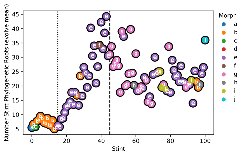
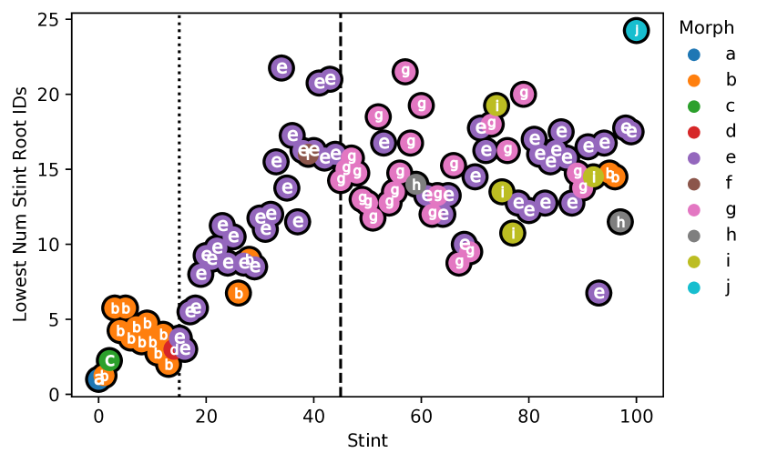
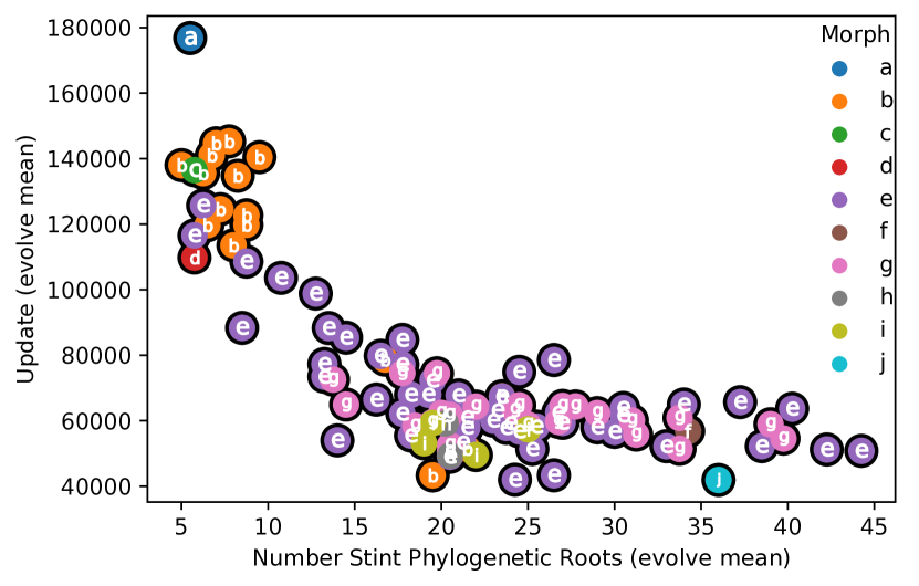
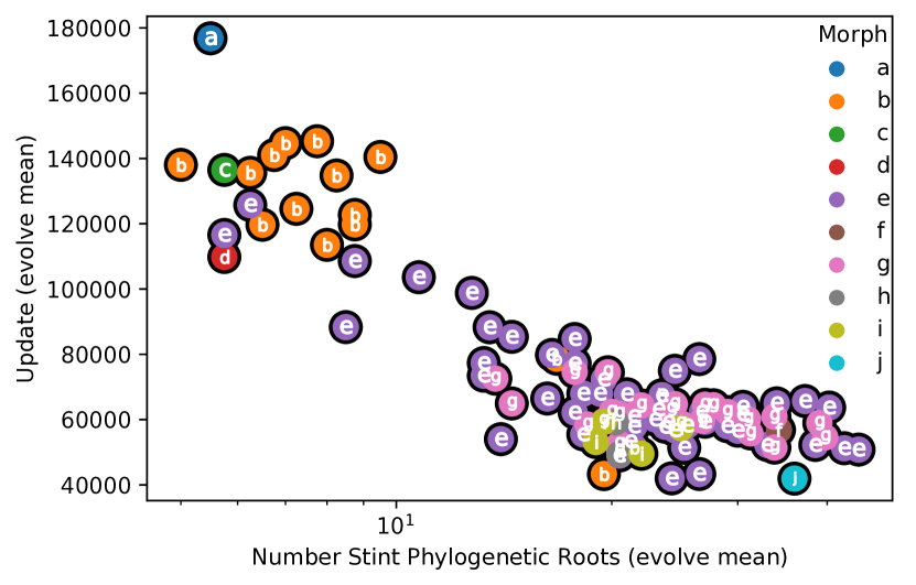
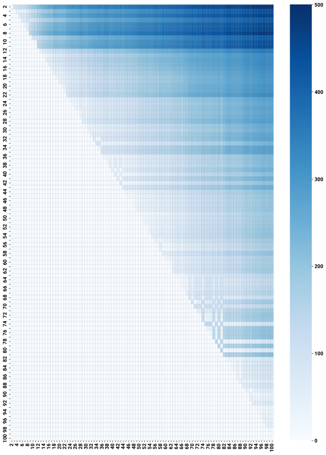
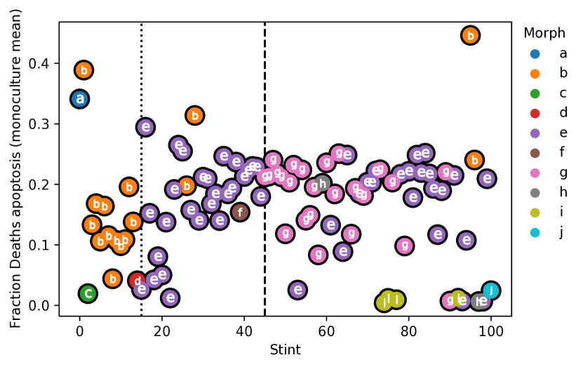
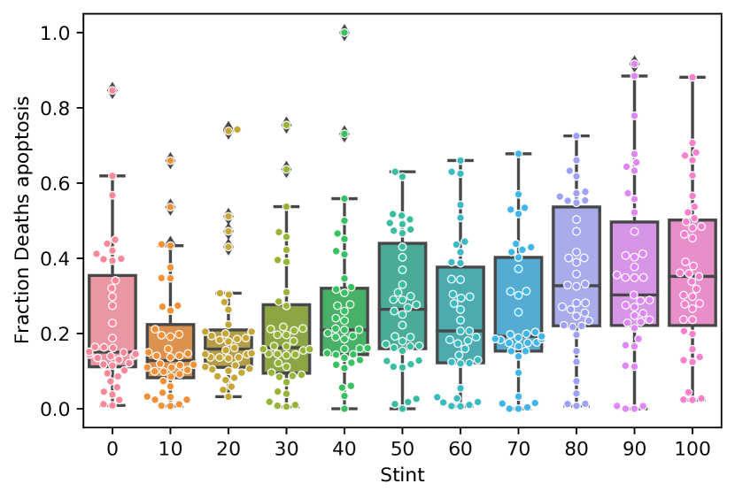
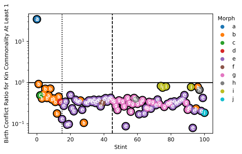
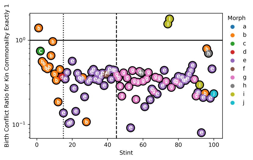
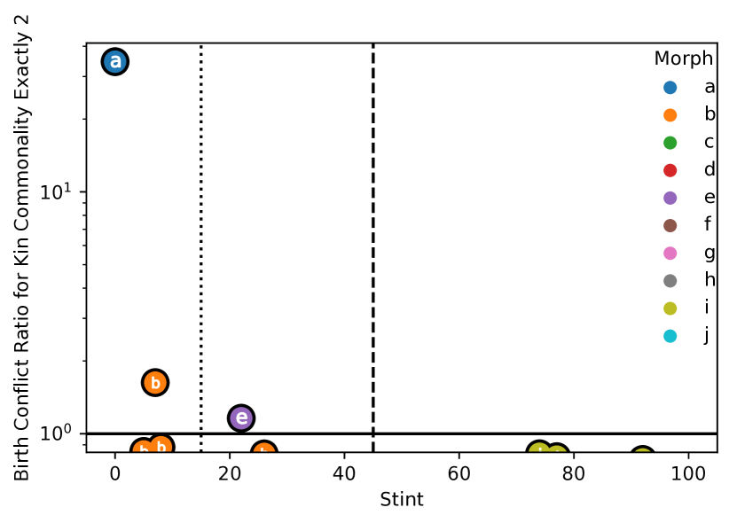
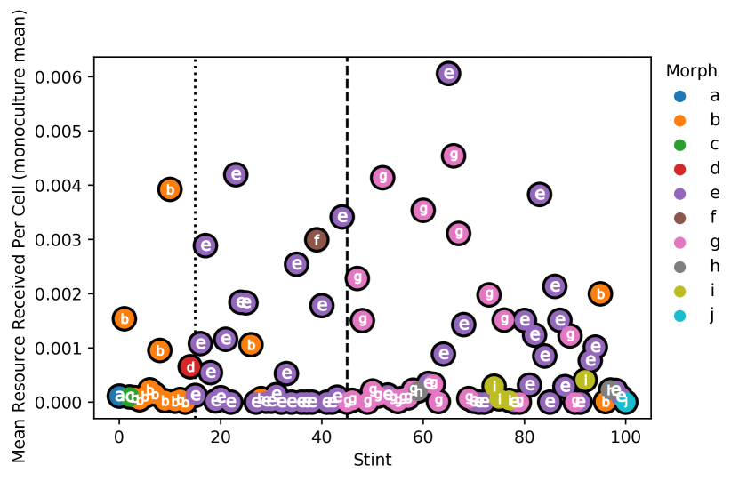
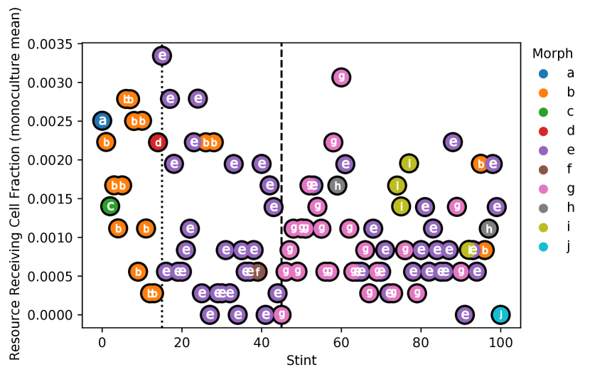
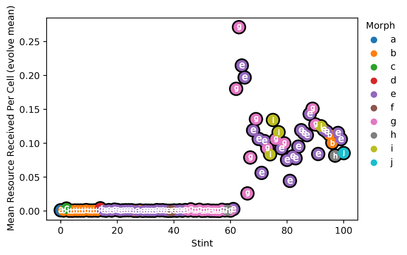
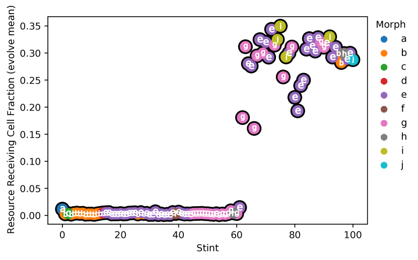
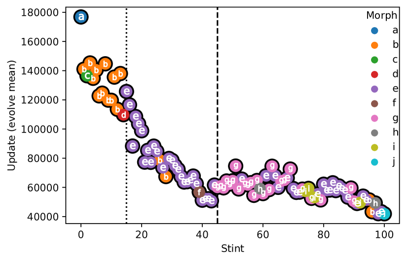
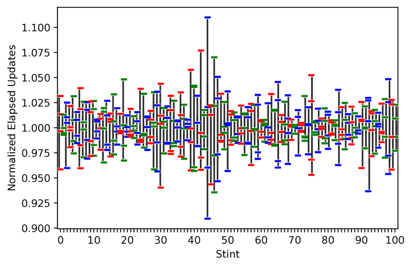
tmp4\zlabelrotate\zref@extractdefaulttmp4page0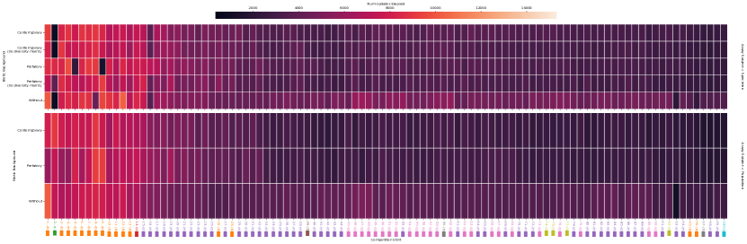
tmp5\zlabelrotate\zref@extractdefaulttmp5page0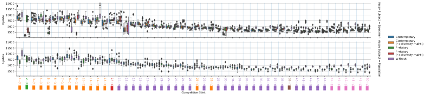
tmp6\zlabelrotate\zref@extractdefaulttmp6page0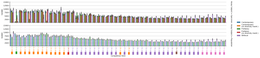
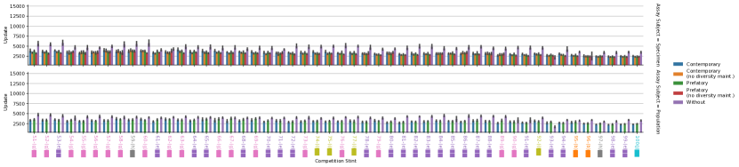
tmp7\zlabelrotate\zref@extractdefaulttmp7page0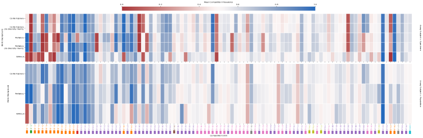
tmp8\zlabelrotate\zref@extractdefaulttmp8page0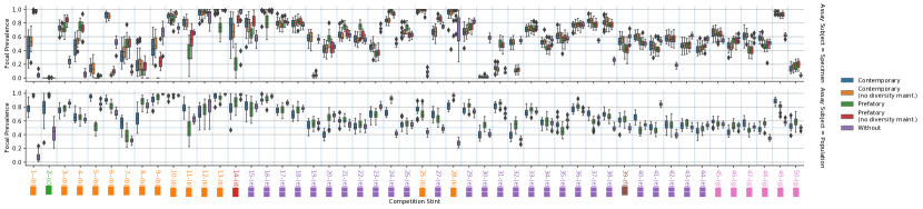
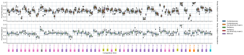
tmp9\zlabelrotate\zref@extractdefaulttmp9page0
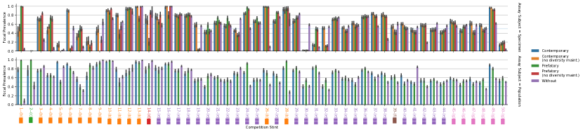
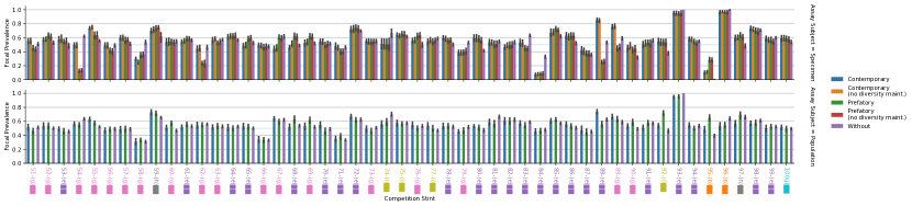
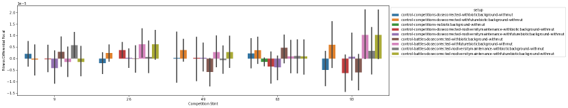
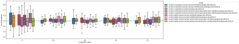
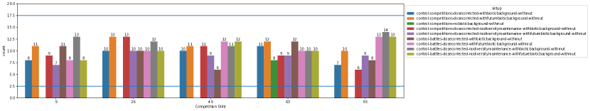
tmp10\zlabelrotate\zref@extractdefaulttmp10page0