A Geometric Decomposition of Finite Games:
Convergence Vs. Recurrence under Exponential Weights

Abstract.

In view of the complexity of the dynamics of learning in games, we seek to decompose a game into simpler components where the dynamics’ long-run behavior is well understood. A natural starting point for this is Helmholtz’s theorem, which decomposes a vector field into a potential and an incompressible component. However, the geometry of game dynamics – and, in particular, the dynamics of exponential / multiplicative weights (EW) schemes – is not compatible with the Euclidean underpinnings of Helmholtz’s theorem. This leads us to consider a specific Riemannian framework based on the so-called Shahshahani metric, and introduce the class of incompressible games, for which we establish the following results: First, in addition to being volume-preserving, the continuous-time EW dynamics in incompressible games admit a constant of motion and are Poincaré recurrent – i.e., almost every trajectory of play comes arbitrarily close to its starting point infinitely often. Second, we establish a deep connection with a well-known decomposition of games into a potential and harmonic component (where the players’ objectives are aligned and anti-aligned respectively): a game is incompressible if and only if it is harmonic, implying in turn that the EW dynamics lead to Poincaré recurrence in harmonic games.

1. Introduction

One of the driving open questions in game-theoretic learning is whether – and under what conditions – players eventually learn to emulate rational behavior through repeated interactions. Put differently, whether a game-theoretic learning process converges to a rational outcome, what type of outcome this could be, under which mode of convergence, in which games, etc. This question has long been one of the mainstays of non-cooperative game theory, and it has recently received increased attention owing to a surge of breakthrough applications in machine learning and AI, from generative adversarial networks, to multi-agent reinforcement learning and online ad auctions.

Depending on the precise context, this question may admit a wide range of answers, from positive to negative. Starting with the positive, a folk result states that if the players of a finite game follow a no-regret learning process, the players’ empirical frequency of play converges in the long run to the set of coarse correlated equilibria – also known as the game’s Hannan set [29]. This result has been pivotal for the development of the field because no-regret play can be achieved through fairly simple myopic processes like the exponential / multiplicative weights (EW) update scheme [83, 58, 7, 8] and its many variants [71, 76, 79]. On the downside however n(itn) this convergence result does not concern the actual strategies employed by the players day-to-day; and n(itn) in many games, the notion of a CCE can lead to outcomes that fail even the weakest axioms of rationalizability. For example, as was shown by Viossat & Zapechelnyuk [82], players may enjoy negative regret for all time, but still play only strictly dominated strategies for the entire horizon of play.

This takes us to the negative end of the spectrum. If we focus on the evolution of the players’ strategies, a series of well-known impossibility results by Hart & Mas-Colell [31, 32] have established that there are no uncoupled learning dynamics – deterministic or stochastic, in either continuous or discrete time – that converge to Nash equilibrium (NE) in all games from any initial condition. In turn, this lends further weight to the question of determining in which games a learning process converges to Nash equilibrium in the day-to-day sense, and in which it does not.

In this regard, the class of games with arguably the strongest convergence guarantees is the class of potential games [66]. Here, the dynamics of EW methods are known to converge, in both continuous and discrete time, and even when the players only have bandit, payoff-based information at their disposal [37, 33]. By contrast, in two-player, zero-sum games with fully mixed equilibria (like Matching Pennies) the standard implementation of the EW algorithm diverges, even with perfect, mixed payoff observations [64]; the so-called “optimistic” variant of Rakhlin & Sridharan [71] converges at a geometric rate if run with perfect payoff observations [85] but diverges if such information is not available [38, 39, 40]; and, finally, the continuous-time version of the EW dynamics – the replicator dynamics –  is Poincaré recurrent, i.e., the trajectory of play returns infinitely close to where it started, infinitely often [69, 63].

Going back to the two classes of games above, potential games are quite special in that the players’ incentives are aligned (their externalities are positive); on the other hand, in two-player zero-sum games, the players’ incentives are anti-aligned (externalities are negative). Largely motivated by this observation, Candogan et al. [14] introduced a principled framework of decomposing a game into a potential and a harmonic component: the potential component of the game captures interactions that amount to a common interest game, while the harmonic component captures the conflicts between the players’ interests. In this way, the decomposition of Candogan et al. [14] effectively maps all games to a spectrum ranging from fully aligned (when the harmonic component of the game is zero) to fully anti-aligned (when the potential component is zero).

Building on this decomposition, a natural question that arises is whether a similar conclusion can be drawn for the players’ learning dynamics. Specifically, focusing for concreteness on continuous time (which eliminates complications related to the players’ hyperparameters or feedback structure), a key question is whether the space of games can be likewise mapped to a “convergence spectrum”, with (global) convergence on one end, and global non-convergence / Poincaré recurrence on the other. A version of this question was already treated in a series of follow-up works by Candogan et al. [16, 15, 17] who showed that the best-response dynamics remain convergent in slight perturbations of potential games. However, moving further toward the class of harmonic games hit an important obstacle, and has remained an open question since the original work of Candogan et al. [14]: except for some special cases, the behavior of the replicator dynamics in harmonic games is not well understood.

Our contributions

In view of the above, our paper’s overarching objective is to derive a dynamics-driven decomposition of games – and, in so doing, to shed light on the dynamics of harmonic games. Motivated by Helmholtz’s theorem for the decomposition of vector fields into a potential and an incompressible, divergence-free component, we first seek to define a class of incompressible games at the opposite end of potential games. However, the geometry of the dynamics turns out to be incompatible with the standard Euclidean geometry of the simplex, so we are led to consider a nonlinear Riemannian structure on the simplex, the Shahshahani metric [75]. This ends up complicating the construction significantly, but it allows us to show that the class of incompressible games that we introduce has the characteristic property that the players’ learning dynamics are volume-preserving (i.e., a set of initial conditions does not decrease in volume relative to the Shahshahani metric).

As a consequence of this, the class of incompressible games is shown to exhibit two fairly unexpected properties:

1. A game is harmonic if and only if it is incompressible, and the decomposition of a game into a potential and incompressible component (relative to the Shahshahani metric) is equivalent to that of Candogan et al. [14].

2. Incompressible games are conservative, i.e., the dynamics admit a constant of motion.

Both properties are surprising, for different reasons. The first, because harmonic and incompressible games have completely different origins: the former is coming from the combinatorial decomposition of Candogan et al. [14], the latter from the kernel of the Shahshahani divergence operator, so there is no reason to expect these notions to coincide. The second, because volume preservation and constants of motion are two complementary and independent properties, so the fact that the former implies the latter is quite mysterious.

Building further on the above, we also show that the EW dynamics are Poincaré recurrent in harmonic games. By itself, this provides a partial answer to the open-ended question of whether harmonic games should be placed in the non-convergent end of the spectrum [14]. Moreover, to the best of our knowledge, Poincaré recurrence in the context of game-theoretic learning has been so far established only in zero-sum games with a fully mixed equilibrium and variations of the above [12, 63, 69]. Seeing as harmonic games are related to zero-sum games (though neither property implies or is implied by the other, cf. Remark D.2), this result identifies an important new class of games where no-regret learning in continuous time fails to converge.

Related work

Before the general definition of harmonic games by Candogan et al. [14], specific instances thereof were already studied in the context of cyclic games, the battle of the sexes, buyer/seller games, and crime deterrence games [36, 78, 27, 23, 18]. Building on these early works, Wang et al. [84], Li et al. [57], Abdou et al. [1] proposed a weighted versions of the decomposition by Candogan et al. [14] based on different inner products on the space of games. Cheng et al. [19] proposed in particular a concise derivation of the decomposition of Candogan et al. [14] with applications to (network) evolutionary games and near-potential games. Hwang & Rey-Bellet [42] present a projection-based decomposition method, equivalent to that of Candogan et al. [14] for finite games and that applies also to mixed extensions of normal form games with continuous action spaces.

On the interplay between decomposition methods and dynamics, beyond the already mentioned follow-up works by Candogan et al. [16, 15, 17] on near-potential games, Cheung & Tao [20] applied volume analysis techniques to the canonical decomposition of a game into zero-sum and coordination components [45, 9] to characterize bimatrix games where standard classes of no-regret learning exhibit Lyapunov chaos. More recently, Letcher et al. [55] employed a decomposition argument to design a novel algorithm for finding stable fixed points in differentiable games. The machinery we develop in this work connects the differential-geometric Hodge/Helmholtz decomposition to a constrained setting, thus providing a partial answer to an open question raised in Letcher et al. [55]; however, there is a key difference between the spirit of our approach and that of Letcher et al. [55], that we discuss in Section E.1.

To the best of our knowledge, the only other works in the literature that study the dynamics of harmonic games are the papers by Li et al. [56] and Cheng et al. [19], which discuss a dynamical equivalence between basis games and evolutionary harmonic games. Except for these works, we are not aware of a similar approach in the literature.

2. Preliminaries

2.1. Elements of game theory

To fix notation, we begin by recalling some basics from game theory, roughly following Fudenberg & Tirole [28]. First, a finite game in normal form consists of a finite set of players $i\in\mathcal{N}\equiv\{1,\dotsc,N\}$, each equipped with (it n) a finite set of actions – or pure strategies – indexed by $\alpha_{i}\in\mathcal{A}_{i}=\{0,1,\dotsc,m_{i}\}$ (so $\lvert\mathcal{A}_{i}\rvert=m_{i}+1$); and (it n) a payoff function $u_{i}\colon\prod_{j}\mathcal{A}_{j}\to\mathbb{R}$, which determines the player’s reward $u_{i}(\alpha)$ at a given action profile $\alpha=(\alpha_{1},\dotsc,\alpha_{N})$. Collectively, we will write $\mathcal{A}=\prod_{i}\mathcal{A}_{i}$ for the game’s action space and $\Gamma\equiv\Gamma(\mathcal{N},\mathcal{A},u)$ for the game with primitives as above.

During play, players may randomize their choices by playing mixed strategies, i.e., probability distributions $x_{i}\in\mathcal{X}_{i}\coloneqq\operatorname{\operatorname{\Delta}}(\mathcal{A}_{i})$ over $\mathcal{A}_{i}$. In this case, we will write $x_{i\alpha_{i}}$ for the probability with which player $i\in\mathcal{N}$ selects $\alpha_{i}\in\mathcal{A}_{i}$ under $x_{i}$, and we will identify $\alpha_{i}\in\mathcal{A}_{i}$ with the mixed strategy that assigns all weight to $\alpha_{i}$ (thus justifying the terminology “pure strategies”). Then, writing $x=(x_{i})_{i\in\mathcal{N}}$ for the players’ strategy profile and $\mathcal{X}=\prod_{i}\mathcal{X}_{i}$ for the game’s strategy space, the players’ mixed payoffs under $x\in\mathcal{X}$ will be $u_{i}(x)\coloneqq\operatorname{\mathbb{E}}_{#1}[u_{i}(\alpha)]=\sum\nolimits_{\alpha\in\mathcal{A}}u_{i}(\alpha)\,x_{\alpha}$ where, in a slight abuse of notation, we write $x_{\alpha}\equiv\prod_{i}x_{i\alpha_{i}}$ for the joint probability of playing $\alpha\in\mathcal{A}$ under $x$.

For notational convenience, we will also write $(x_{i};x_{-i})=(x_{1},\dotsc,x_{i},\dotsc,x_{N})$ for the strategy profile where player $i$ plays $x_{i}\in\mathcal{X}_{i}$ against the strategy $x_{-i}\in\mathcal{X}_{-i}\coloneqq\prod_{j\neq i}\mathcal{X}_{j}$ of all other players (and likewise for pure strategies). In this notation, each player’s individual payoff field is defined as

$$v_{i}(x)=(u_{i}(\alpha_{i};x_{-i}))_{\alpha_{i}\in\mathcal{A}_{i}}$$ (1)

so the mixed payoff of player $i\in\mathcal{N}$ under $x\in\mathcal{X}$ becomes

$$u_{i}(x)=\sum\nolimits_{\alpha_{i}\in\mathcal{A}_{i}}u_{i}(\alpha_{i};x_{-i})\,x_{i\alpha_{i}}=v_{i}(x)^{\top}\cdot x_{i}.$$ (2)

In view of the above, the aggregate payoff field $v(x)=(v_{1}(x),\dotsc,v_{N}(x))$ collectively captures all strategic information of the game, so we will use it interchangeably as a more compact description of the game $\Gamma(\mathcal{N},\mathcal{A},u)$.

The most widely used solution concept in game theory is that of a Nash equilibrium (NE), i.e., a strategy profile $x^{\ast}\in\mathcal{X}$ which discourages unilateral deviations in the sense that

$$u_{i}(x^{\ast})\geq u_{i}(x_{i};x^{\ast}_{-i})\quad\text{for all $x_{i}\in\mathcal{X}_{i}$, $i\in\mathcal{N}$}.$$ (NE)

Since a game’s equilibria only depend on pairwise payoff comparisons, two games $\Gamma(\mathcal{N},\mathcal{A},u)$ and $\Gamma^{\prime}(\mathcal{N},\mathcal{A},u^{\prime})$ are called strategically equivalent – and we write $\Gamma\sim\Gamma^{\prime}$ – if, for all $\alpha,\beta\in\mathcal{A}$ and all $i\in\mathcal{N}$, we have

$$u^{\prime}_{i}(\beta_{i};\alpha_{-i})-u^{\prime}_{i}(\alpha_{i};\alpha_{-i})=u_{i}(\beta_{i};\alpha_{-i})-u_{i}(\alpha_{i};\alpha_{-i}).$$ (3)

Clearly, strategically equivalent games yield identical payoff comparisons per player, so they share the same set of Nash equilibria.

2.2. A strategic decomposition of games

One of the most important classes of normal form games is the class of potential games (PGs). First introduced by Monderer & Shapley [66], potential games enjoy several properties of interest – existence of equilibria in pure strategies, lack of best-response cycles, convergence of standard learning dynamics and algorithms, etc. Formally, a finite game $\Gamma$ is said to be a potential game if it admits a potential function $\phi\colon\mathcal{X}\to\mathbb{R}$ such that

$$u_{i}(\beta_{i};\alpha_{-i})-u_{i}(\alpha_{i};\alpha_{-i})=\phi(\beta_{i};\alpha_{-i})-\phi(\alpha_{i};\alpha_{-i})$$ (PG)

for all $\alpha,\beta\in\mathcal{A}$ and all $i\in\mathcal{N}$. Equivalently, in terms of mixed payoffs, this condition can be rewritten in differential form as

$$v(x)^{\top}(x^{\prime}-x)=\kern 0.0pt\partial\mkern-1.0mu{}\phi(x;x^{\prime}-x)\quad\text{for all $x,x^{\prime}\in\mathcal{X}$}$$ (4)

where $\phi(x)\coloneqq\sum\nolimits_{\alpha}\phi(\alpha)\,x_{\alpha}$ denotes the mixed extension of $\phi$ to $\mathcal{X}$, and $\kern 0.0pt\partial\mkern-1.0mu{}\phi(x;z)=\lim_{t\to 0^{+}}[\phi(x+tz)-\phi(x)]/t$ denotes the (one-sided) directional derivative of $\phi$ at $x$ along $z$.

PG capture strategic interactions with “aligned incentives” (as in common interest and congestion games). Dually to this, Candogan et al. [14] introduced the class of harmonic games (HGs) as those with “anti-aligned incentives”, viz.

$$\sum\nolimits_{i\in\mathcal{N}}\sum\nolimits_{\beta_{i}\in\mathcal{A}_{i}}[u_{i}(\beta_{i};\alpha_{-i})-u_{i}(\alpha_{i};\alpha_{-i})]=0$$ (HG)

for all $\alpha\in\mathcal{A}$, meaning that the net incentive to deviate toward and away from any pure strategy profile is zero. In contrast to potential games, harmonic games generically do not admit pure equilibria and they possess non-terminating best-response paths, so they can be seen as “orthogonal” to potential games.

This observation was made precise by Candogan et al. [14] who showed that any finite game admits the strategic decomposition

$$\Gamma=\Gamma_{\!\textup{pot}}+\Gamma_{\!\textup{harm}}$$ (5)

where $\Gamma_{\!\textup{pot}}$ is potential and $\Gamma_{\!\textup{harm}}$ is harmonic. This decomposition is achieved by representing $\Gamma$ as a weighted preference graph, endowing said graph with a specific, Euclidean-like structure, and using the combinatorial Helmholtz decomposition theorem [43] to obtain (5). In general, this decomposition is only unique up to strategic equivalence: more precisely, if $\Gamma$ admits the alternative decomposition $\Gamma=\Gamma_{\!\textup{pot}}^{\prime}+\Gamma_{\!\textup{harm}}^{\prime}$ with $\Gamma_{\!\textup{pot}}^{\prime}$ potential and $\Gamma_{\!\textup{harm}}^{\prime}$ harmonic, then $\Gamma_{\!\textup{pot}}^{\prime}$ is strategically equivalent to $\Gamma_{\!\textup{pot}}$ and $\Gamma_{\!\textup{harm}}^{\prime}$ to $\Gamma_{\!\textup{harm}}$. We will return to this decomposition later.

3. Learning via exponential weights

Throughout our paper, we will focus on dynamic learning proceses where the players seek to myopically improve their individual payoffs over time. A crucial requirement in this regard is the minimization of the players’ regret, that is, the difference between a player’s cumulative payoff and the player’s best strategy in hindsight. Formally, assuming that play evolves in continuous time, the regret of a player $i\in\mathcal{N}$ relative to a sequence of play $x(t)\in\mathcal{X}$, $t\geq 0$, is defined as

$$\operatorname{Reg}_{i}(T)=\max_{p_{i}\in\mathcal{X}_{i}}\int_{0}^{T}[u_{i}(p_{i};x_{-i}(t))-u_{i}(x(t))]\>dt$$ (6)

and we say that player $i$ has no regret if $\operatorname{Reg}_{i}(T)=o(T)$.

The archetypal method for attaining no regret is the so-called exponential / multiplicative weights (EW) update scheme, whereby an action is played with probability that is exponentially proportional to its cumulative payoff. This simple stimulus-response model goes back to Vovk [83], Littlestone & Warmuth [58] and Auer et al. [7], and, in our setting, it boils down to the dynamics

$$y_{i}(t)=y_{i}(0)+\int_{0}^{t}\!\!\!v_{i}(x(t))\>dt\qquad x_{i}(t)=\operatorname{LC}_{i}(y_{i}(t))$$ (EW)

where $\operatorname{LC}_{i}\colon\mathbb{R}^{\mathcal{A}_{i}}\to\mathcal{X}_{i}$ denotes the logit choice map

$$\operatorname{LC}_{i}(y_{i})=\frac{(\exp(y_{i\alpha_{i}}))_{\alpha_{i}\in\mathcal{A}_{i}}}{\sum_{\alpha_{i}\in\mathcal{A}_{i}}\exp(y_{i\alpha_{i}})}.$$ (7)

As was first shown by [79, 48], the dynamics (EW) enjoy a constant, $\operatorname{\mathcal{O}}(1)$ regret bound, namely

$$\operatorname{Reg}_{i}(T)\leq\log\lvert\mathcal{A}_{i}\rvert.$$ (8)

Owing to this remarkable regret guarantee, (EW) and its variants have become the “gold standard” for no-regret learning; for an introduction to the vast corpus of literature surrounding the topic, we refer the reader to [6, 76, 52].

One last important property of (EW) is that, by a standard calculation, the evolution of the players’ mixed strategies $x_{i}\in\mathcal{X}_{i}$ under (EW) follows the replicator dynamics of Taylor & Jonker [81], viz.

$$\dot{x}_{i\alpha_{i}}=x_{i\alpha_{i}}[u_{i}(\alpha_{i};x_{-i})-u_{i}(x)]$$ (RD)

The replicator dynamics (RD) comprise the cornerstone of evolutionary game theory and, as such, their rationality properties have been the subject of intense study in the literature, cf. [37, 86, 74] and references therein. For all these reasons, the dynamics (EW)/(RD) will be our main focus in the sequel.

4. The geometry of exponential weights

We now turn to our overarching objective, that is, to identify in which classes of games we can expect the dynamics of exponential / multiplicative weights to converge, and in which classes we cannot. Our main tool for this will be Helmholtz’s theorem, a simpler variant of the Hodge decomposition theorem, itself one of the most foundational results in differential geometry [24, 34, 11].

To set the stage for the analysis to come, we begin by presenting the original Helmholtz decomposition of vector fields in the Euclidean setting of $\mathbb{R}^{n}$. Subsequently, we develop the geometric background needed to define and describe the class of incompressible games later in this section.

4.1. The Helmholtz decomposition

Consider the dynamics

$$\dot{x}=F(x)$$ (Dyn)

induced by some sufficiently smooth vector field $F\colon\mathbb{R}^{n}\to\mathbb{R}^{n}$ on $\mathbb{R}^{n}$. Helmholtz’s theorem states that, if $F$ decays at infinity as $\lVert F(x)\rVert=o(\lVert x\rVert^{-2})$, it can be resolved as

$$F(x)=\nabla\phi(x)+B(x)$$ (9)

where $\phi\colon\mathbb{R}^{n}\to\mathbb{R}$ is a scalar potential for $F$ and the vector field $B\colon\mathbb{R}^{n}\to\mathbb{R}^{n}$ is incompressible, i.e., it has vanishing divergence:

$$\nabla\!\cdot\!B(x)\coloneqq\sum\nolimits_{a=1}^{n}\partial B_{a}/\partial x_{a}=0\quad\text{for all $x\in\mathbb{R}^{n}$}.$$ (10)

The decomposition (9) is known as the Helmholtz decomposition of $F$, and it is particularly important from a dynamical standpoint because its two components exhibit “orthogonal” behaviors in terms of convergence. More precisely, by standard Lyapunov arguments, the flow $\dot{x}=\nabla\phi(x)$ of the gradient component of $F$ generically converges to the critical set of $\phi$ [46]. On the other hand, Liouville’s theorem shows that the flow $\dot{x}=B(x)$ of the incompressible component of $F$ is volume-preserving, so it does not admit any stable attractors (asymptotically stable points or limit cycles). In this sense, the potential component of $F$ represents the convergent part of (Dyn), while the incompressible component encapsulates the non-convergent part thereof.

In view of the above, a natural idea to characterize convergent and non-convergent behaviors under (RD) would be to apply Helmholtz’s theorem to the vector field

$$v^{\sharp}_{i\alpha_{i}}(x) \coloneqq x_{i\alpha_{i}}[u_{i}(\alpha_{i};x_{-i})-u_{i}(x)]$$

$$=x_{i\alpha_{i}}\left[v_{i\alpha_{i}}(x)-\sum\nolimits_{\beta_{i}\in\mathcal{A}_{i}}x_{i\beta_{i}}v_{i\beta_{i}}(x)\right]$$ (11)

of (RD) that describes the evolution of the players’ mixed strategies under (EW). Unfortunately however, a direct decomposition of $v^{\sharp}$ into a potential and incompressible component – in the sense of Helmholtz’s theorem – is not well-aligned with the properties of the underlying game.

To see this, consider the single-player game with actions “$\mathtt{A}$” and “$\mathtt{B}$” and payoffs $u(\mathtt{A})=0$ and $u(\mathtt{B})=1$. Since there is only one player, the game admits the potential function $\phi(x)=u(x)=0\cdot x_{\mathtt{A}}+1\cdot x_{\mathtt{B}}=x_{\mathtt{B}}$, so it is a potential one. However, the replicator dynamics for this toy example are

$$\dot{x}_{\mathtt{A}} =v^{\sharp}_{\mathtt{A}}(x)\equiv x_{\mathtt{A}}[0-u(x)] =-x_{\mathtt{A}}x_{\mathtt{B}}$$ (12)

$$\dot{x}_{\mathtt{B}} =v^{\sharp}_{\mathtt{B}}(x)\equiv x_{\mathtt{B}}[1-u(x)] =x_{\mathtt{B}}-x_{\mathtt{B}}^{2}$$

and a simple check shows that $\cramped{\partial_{\mathtt{B}}v^{\sharp}_{\mathtt{A}}}=-x_{\mathtt{A}}\neq 0=\cramped{\partial_{\mathtt{A}}v^{\sharp}_{\mathtt{B}}}.$ By a routine application of Poincaré’s lemma, this further shows that $v^{\sharp}(x)$ is not the gradient of a potential function in the sense of (9). As a result, the game is not a potential one in the sense of Helmholtz’s theorem.

The above shows that the property of (RD) being a potential system in the sense of Helmholtz (which is more relevant from a dynamical standpoint) is not aligned with the property of admitting a potential in the sense of Monderer & Shapley [66] (which is more relevant from a game-theoretic standpoint). In view of this, our goal in the sequel will be to bridge this gap by means of an alternate decomposition in which the discrepancy between “strategically potential” and “dynamically potential” games disappears.

4.2. The geometry of the replicator dynamics

The starting point of our analysis is the observation that, under (RD), players track the direction of steepest individual payoff ascent; however, this ascent is not defined relative to the standard Euclidean geometry of $\mathbb{R}^{n}$ (which underlies Helmholtz’s theorem), but relative to a non-Euclidean structure known as the Shahshahani metric.

To make this precise, we begin by introducing the notion of a Riemannian metric, a fundamental geometric concept which generalizes the ordinary Euclidean scalar product between vectors. Formally, a Riemannian metric on an open set $\mathcal{U}$ of $\mathbb{R}^{n}$ is a smooth assignment of an inner product to each $x\in\mathcal{U}$, i.e., a family of bilinear pairings $\langle\kern 1.0pt\boldsymbol{\cdot}\kern 1.0pt,\kern 1.0pt\boldsymbol{\cdot}\kern 1.0pt\rangle_{x}$, $x\in\mathcal{U}$, that satisfies the following requirements for all $z,z^{\prime}\in\mathbb{R}^{n}$ and all $x\in\mathcal{U}$:

1. Symmetry: $\langle z,z^{\prime}\rangle_{x}=\langle z^{\prime},z\rangle_{x}$.

2. Positive-definiteness: $\langle z,z\rangle_{x}\geq 0$ with equality iff $z=0$.

This definition can be made more concrete in the standard frame $\{e_{a}\}_{a=1}^{n}$ of $\mathbb{R}^{n}$ by defining the metric tensor of $\langle\kern 1.0pt\boldsymbol{\cdot}\kern 1.0pt,\kern 1.0pt\boldsymbol{\cdot}\kern 1.0pt\rangle_{x}$ as the matrix $g(x)\in\mathbb{R}^{n\times n}$ with entries

$$g_{ab}(x)=\langle e_{a},e_{b}\rangle_{x}\quad\text{for $a,b=1,\dotsc,n$}.$$ (13)

The Shahshahani metric [75] on the positive orthant $\mathbb{R}^{n}_{++}$ of $\mathbb{R}^{n}$ is then defined as

$$g_{ab}(x)=\delta_{ab}/x_{a}\quad\text{for all $x\in\mathbb{R}^{n}_{++}$}$$ (14)

where $\delta_{ab}$ denotes the standard Kronecker delta.

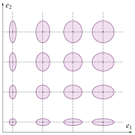
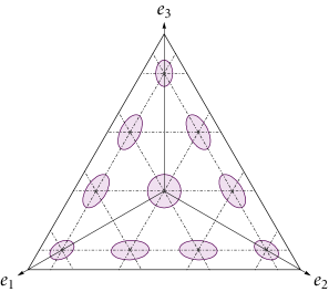
Figure 1. Unit balls on the orthant and the simplex under the Shahshahani metric (left and right respectively). Notice how the Shahshahani metric distorts distances near the boundary and flattens the balls along the axis that they are closest to.

Importantly, the Shahshahani unit spheres $\mathbb{S}_{x}\coloneqq\{z\in\mathbb{R}^{n}:\langle z,z\rangle_{x}=1\}$ at $x$ become increasingly flattened along the $x_{a}$-axis as $x_{a}\to 0$ (for an illustration, Fig. 1 below). Because of this distortion, the notion of a “gradient” and the “direction of steepest ascent” must both be redefined to account for the fact that all displacements of interest take place in the (open) unit simplex $\operatorname{\operatorname{\Delta}}^{\!\circ}=\{x\in\mathbb{R}^{n}_{++}:\sum_{a}x_{a}=1\}$ of $\mathbb{R}^{n}$.

To do so, we proceed as follows: Given a differentiable function $f\colon\mathbb{R}^{n}_{++}\to\mathbb{R}$, we define the its Shahshahani gradient along $\operatorname{\operatorname{\Delta}}^{\!\circ}$ as the vector field $\operatorname{grad}f(x)$ which is (itn) tangent to $\operatorname{\operatorname{\Delta}}^{\!\circ}$; and (itn) satisfies the defining relation

$$\langle\operatorname{grad}f(x),z\rangle_{x}=\kern 0.0pt\partial\mkern-1.0mu{}f(x;z)$$ (15)

for all $x\in\operatorname{\operatorname{\Delta}}^{\!\circ}$ and all $z$ that are tangent to $\operatorname{\operatorname{\Delta}}^{\!\circ}$ (i.e., $\sum_{a}z_{a}=0$ in the standard basis of $\mathbb{R}^{n}$). This relation clearly mirrors the corresponding Euclidean definition $\nabla f(x)^{\top}\cdot z=\kern 0.0pt\partial\mkern-1.0mu{}f(x;z)$, and as we show in Appendix A, it can be equivalently characterized as the direction of “steepest ascent”, namely

$$\textstyle\operatorname{grad}f(x)\propto\operatorname*{arg\,max}\big{\{}\kern 0.0pt\partial\mkern-1.0mu{}f(x;z):z\in\mathbb{S}_{x},\sum_{a}z_{a}=0\big{\}}.$$ (16)

In other words, $\operatorname{grad}f(x)$ points in the direction that maximizes the rate of increase of $f$ at $x$ among all vectors that are tangent to $\operatorname{\operatorname{\Delta}}^{\!\circ}$ and have unit Shahshahani norm.

Now, to obtain an explicit expression for $\operatorname{grad}f(x)$ in the standard basis of $\mathbb{R}^{n}$, note that (15) gives

$$\sum_{a=1}^{n}\frac{[\operatorname{grad}f(x)]_{a}\,z_{a}}{x_{a}}=\sum_{a=1}^{n}\frac{\partial f}{\partial x_{a}}z_{a}$$ (17)

for all $z\in\mathbb{R}^{n}$ such that $\sum_{a}z_{a}=0$. Then, as we show in Appendix C, solving this equation yields the expression

$$[\operatorname{grad}f(x)]_{a}=x_{a}\left[\frac{\partial f}{\partial x_{a}}-\sum\nolimits_{b=1}^{n}x_{b}\frac{\partial f}{\partial x_{b}}\right].$$ (18)

This last expression is strongly reminiscent of the vector field $v^{\sharp}$ defining (RD), a link which we make precise below.

Now, to return to a game-theoretic context, let $\mathcal{X}^{\circ}_{i}$ denote the relative interior of the mixed strategy space $\mathcal{X}_{i}\equiv\operatorname{\operatorname{\Delta}}(\mathcal{A}_{i})$, and endow $\mathbb{R}_{++}^{\mathcal{A}_{i}}$ with the Shahshahani metric as above. We then define the individual payoff gradient of player $i\in\mathcal{N}$ as the vector field $\operatorname{grad}_{i}u_{i}$ which is (itn) tangent to $\mathcal{X}^{\circ}_{i}$; and (itn) satisfies the defining relation

$$\langle\operatorname{grad}_{i}u_{i}(x),z_{i}\rangle=\kern 0.0pt\partial\mkern-1.0mu{}u_{i}(x;z_{i})$$ (19)

for all $z_{i}\in\mathbb{R}^{\mathcal{A}_{i}}$ that are tangent to $\mathcal{X}^{\circ}_{i}$ at $x_{i}$ (that is, $\sum_{\alpha_{i}\in\mathcal{A}_{i}}z_{i\alpha_{i}}=0$). Then, by invoking the explicit expression (18) and observing that $\partial u_{i}/\partial x_{i\alpha_{i}}=u_{i}(\alpha_{i};x_{-i})$, we finally obtain the following geometric characterization of the replicator dynamics.

Proposition 1.

Under the Shahshahani metric, (RD) is equivalent to the steepest individual payoff ascent dynamics

$$\dot{x}_{i}=\operatorname{grad}_{i}u_{i}(x)$$ (20)

i.e., $v^{\sharp}_{i}(x)=\operatorname{grad}_{i}u_{i}(x)$ for all $i\in\mathcal{N}$.

A version of this result appears without proof in [51]; for completeness, we defer the details of the proof of Proposition 1 to Appendix C. What is more important for our purposes is that, as we show in Section C.3, if the game admits a potential in the sense of (PG), combining Propositions 1, 4 and 15 shows that (RD) is a Shahshahani potential system, that is, $\dot{x}=\operatorname{grad}\phi$.

As far as we are aware, the closest result to Proposition 1 in the literature is Kimura’s maximum principle [47] which states that, in potential games, (RD) is a Shahshahani gradient system – thus lifting the discrepancy between the “dynamic” and “strategic” notions of potential that arose before. Proposition 1 provides a broad generalization of this principle to the effect that, in any game, players following (EW)/(RD) track the direction of steepest unilateral payoff ascent, provided that displacements are measured relative to the Shahshahani metric.

4.3. Incompressible games

Going back to the Helmholtz decomposition (9), we see that it involves two Euclidean differential operators, the gradient $\nabla\phi$ and the divergence $\nabla\!\cdot\!B$. Eq. 15 shows how to redefine gradients relative to the Shahshahani metric, but the corresponding construction for the divergence is more intricate. The reason for this is that (RD) has an inert degree of freedom along $(1,\dotsc,1)$, so the standard definition of the divergence on the ambient space of the simplex is not appropriate [25, Chap. 6]. To circumvent this, we will introduce a more parsimonious representation of (RD) which has no redundant directions; we do this first in the case of a single player with action set $\mathcal{A}=\{0,1,\dotsc,m\}$, and only reinstate the player index $i\in\mathcal{N}$ toward the end of this section.

To proceed, consider the coordinate transformation

$$\pi_{0}(x_{0},x_{1},\dotsc,x_{m})=(x_{1},\dotsc,x_{m})$$ (21)

which maps the standard unit simplex of $\mathbb{R}^{m+1}$ to the “corner of cube”

$$\mathcal{C}=\{\tilde{x}\in\mathbb{R}^{m}_{+}:\sum_{\mu=1}^{m}\tilde{x}_{\mu}\leq 1\}$$ (22)

of $\mathbb{R}^{m}$ by eliminating $x_{0}$ (i.e., by replacing the constraint “summing to $1$” with “summing to at most $1$”). Then, for all $\mu=1,\dotsc,m$, the dynamics (RD) become

$$\frac{d\tilde{x}_{\mu}}{dt} =\dot{x}_{\mu}=x_{\mu}\left[v_{\mu}(x)-\sum\nolimits_{\alpha=0}^{m}x_{\alpha}v_{\alpha}(x)\right]$$

$$\quad=\tilde{x}_{\mu}\left[\tilde{v}_{\mu}(\tilde{x})-\sum\nolimits_{\nu=1}^{m}\tilde{x}_{\nu}\tilde{v}_{\nu}(\tilde{x})\right]$$ (RD₀)

where, in obvious notation, we set

$$\tilde{v}_{\mu}(\tilde{x})=v_{\mu}(x)-v_{0}(x)\quad\text{for all $\mu=1,\dotsc,m$}.$$ (23)

Seeing as the dynamics evolve in an open set of $\mathbb{R}^{m}$ (as opposed to a hyperplane of $\mathbb{R}^{m+1}$), there is no longer any redundancy in the dynamics’ degrees of freedom. In view of this, we will need to “push forward” the Shahshahani metric from $\mathbb{R}^{m+1}$ to $\mathbb{R}^{m}$ (or, more precisely, the positive orthants thereof) in a way that is compatible with $\pi_{0}$.

To do so, we begin by noting that the preimage of the standard frame $\{\tilde{e}_{\mu}\}_{\mu=1}^{m}$ of $\mathbb{R}^{m}$ restricted to the tangent space $\mathcal{Z}$ of $\operatorname{\operatorname{\Delta}}$ in $\mathbb{R}^{m+1}$ is

$$\pi_{0}^{\ast}(\tilde{e}_{\mu})\coloneqq e_{\mu}-e_{0}\quad{\text{for all $\mu=1,\dotsc,m$}}\,.$$ (24)

Accordingly, as we explain in more detail in Appendix B, the metric transported in this way to the interior $\mathcal{C}^{\circ}$ of $\mathcal{C}$ will be given by the metric tensor

$$\tilde{g}_{\mu\nu}(\tilde{x})=\langle\tilde{e}_{\mu},\tilde{e}_{\nu}\rangle_{\tilde{x}}=\langle e_{\mu}-e_{0},e_{\nu}-e_{0}\rangle_{x}=\frac{\delta_{\mu\nu}}{x_{\mu}}+\frac{1}{x_{0}}$$ (25)

for all $\mu,\nu=1,\dotsc,m$ and all $\tilde{x}\in\mathcal{C}^{\circ}$.

We now have all the ingredients required to define the Shahshahani divergence operator on the interior $\mathcal{C}^{\circ}$ of $\mathcal{C}$. Since $\mathcal{C}^{\circ}$ is an open subset of $\mathbb{R}^{m}$ (which was not the case for the relative interior $\operatorname{\operatorname{\Delta}}^{\!\circ}$ of $\operatorname{\operatorname{\Delta}}$ in $\mathbb{R}^{m+1}$), the Shahshahani divergence of a vector field $\tilde{F}\colon\mathcal{C}^{\circ}\to\mathbb{R}^{m}$ may be defined by the Riemannian expression

$$\operatorname{div}\tilde{F}(\tilde{x})\coloneqq\frac{1}{\sqrt{\det\tilde{g}(\tilde{x})}}\sum_{\mu=1}^{m}\frac{\partial}{\partial\tilde{x}_{\mu}}\left(\sqrt{\det\tilde{g}(\tilde{x})}\,\tilde{F}_{\mu}(\tilde{x})\right)$$ (26)

with $\tilde{g}$ given by (25). In particular, when applied to each player’s individual steepest ascent payoff field $v^{\sharp}_{i}(x)=\operatorname{grad}_{i}u_{i}(x)$, the coordinate expression (26) yields

$$\operatorname{div}_{i}v^{\sharp}_{i}(\tilde{x})=\frac{1}{\sqrt{\det\tilde{g}_{i}(\tilde{x}_{i})}}\sum_{\mu_{i}=1}^{m_{i}}\frac{\partial}{\partial\tilde{x}_{i\mu_{i}}}\left(\sqrt{\det\tilde{g}_{i}(\tilde{x}_{i})}\,v^{\sharp}_{i\mu_{i}}(\tilde{x})\right)$$ (27)

where, in view of Sections 4.1 and 23, and in a slight – but suggestive – abuse of notation, we have set

$$v^{\sharp}_{i\mu_{i}}(\tilde{x})\coloneqq\tilde{x}_{i\mu_{i}}\left[\tilde{v}_{i\mu_{i}}(\tilde{x})-\sum\nolimits_{\nu_{i}=1}^{m_{i}}\tilde{x}_{i\nu_{i}}\tilde{v}_{i\nu_{i}}(\tilde{x})\right]$$ (28)

with $\tilde{v}_{i\mu_{i}}(\tilde{x})=v_{i\mu_{i}}(x)-v_{i,0}(x)$ defined as in (23) for all $i\in\mathcal{N}$ and all $\mu_{i}=1,\dotsc,m_{i}$.

With all this in hand, we are finally in a position to define incompressible games:

Definition 1.

A finite game $\Gamma\equiv\Gamma(\mathcal{N},\mathcal{A},u)$ will be called incompressible relative to the Shahshahani metric when

$$\operatorname{div}v^{\sharp}(\tilde{x})\coloneqq\sum\nolimits_{i\in\mathcal{N}}\operatorname{div}_{i}v^{\sharp}_{i}(\tilde{x})=0.$$ (29)

We should stress here that Definition 1 is motivated by purely geometric considerations, and provides a “complement” to the class of potential games in a geometric context. In this regard, our goal in the sequel will be to use this definition as the basis for a Helmholtz-like decomposition relative to the Shahshahani metric and, in so doing, we understand the dynamic and game-theoretic implications of such a decomposition. We carry this out in the next section.

5. Analysis and results

5.1. A geometric decomposition of games

To recap, our analysis so far has highlighted the relation between the Shahshahani metric and learning under (EW) / (RD). On that account, the first question that we seek to address is whether Helmholtz’s theorem can be extended to the present context, and whether such a decomposition resolves the dynamic/strategic disconnect that underlies the “vanilla” Helmholtz decomposition. Our first result below answers this question in the positive.

Theorem 1.

Every finite game $\Gamma$ can be decomposed as

$$\Gamma=\Gamma_{\!\textup{pot}}+\Gamma_{\!\textup{inc}}$$ (30)

where $\Gamma_{\!\textup{pot}}$ is potential and $\Gamma_{\!\textup{inc}}$ is incompressible. In particular, at the vector field level, we have

$$v^{\sharp}=\operatorname{grad}\phi+B$$ (31)

where $\phi$ is a potential for $\Gamma_{\!\textup{pot}}$ and $B$ is incompressible in the sense of (29).

Theorem 1 comes as a consequence of Theorem 2, which relates harmonic to incompressible games, and which we state later in this section. Because the calculations are fairly lengthy and involved, we defer all relevant details to Appendix D, and we focus here on the game-theoretic implications of Theorem 1.

A first conclusion that can be drawn from Theorem 1 is that the decomposition (30) pinpoints two concrete building blocks of the space of games: potential games and incompressible games. With regard to the potential component, Theorem 1 resolves the dynamic-strategic disconnect that arose when we applied the standard Helmholtz decomposition to (RD): the component $\Gamma_{\!\textup{pot}}$ of (30) also admits a Shahshahani potential in the sense of (15), so there is no longer any mismatch between the two viewpoints.

The role of the incompressible component is less transparent, but it is clarified by the striking equivalence below:

Theorem 2.

A finite game is harmonic if and only if it is incompressible. In particular, up to strategic equivalence, the decompositions (5) and (30) coincide.

This result hinges on a series of geometric calculations involving the explicit coordinate expression of the Shahshahani divergence operator (26); we defer this calculation to Appendix D, where we discuss all relevant details. What is more important for our purposes is that Theorem 2 provides a fairly unexpected – and operationally significant – interpretation of incompressible games: even though incompressible games were introduced solely based on their relation with the Shahshahani metric – and, through that, to the learning dynamics (EW) – they are characterized by the same “negative externalities” property (HG) which states that the net incentive to deviate toward and/or away from any pure strategy profile is zero. As we shall see below, this strategic “conservation of incentives” is mirrored in the evolution of learning in incompressible / harmonic games under (EW).

5.2. Dynamic considerations

We now turn to our paper’s second major objective: understanding the behavior of learning under (EW) in the class of harmonic / incompressible games.

The first thing to note here is that, as in the Euclidean case, incompressibility is inherently tied to volume preservation. However, in contrast to the Euclidean case, volumes must now be measured relative to the Shahshahani metric. The relevant device in our Riemannian setting is the notion of the Shahshahani volume form, defined on the (open) unit simplex $\operatorname{\operatorname{\Delta}}^{\!\circ}$ of $\mathbb{R}^{m+1}$ as

$$\operatorname{vol}(\mathcal{U})=\int_{\pi_{0}(\mathcal{U})}\!\sqrt{\det\tilde{g}(\tilde{x})}\>d\tilde{x}_{1}\dotsm\!\>d\tilde{x}_{m}$$ (32)

where $\mathcal{U}$ is an open subset of $\operatorname{\operatorname{\Delta}}^{\!\circ}$ and $\tilde{g}(\tilde{x})$ is the coordinate representation of the Shahshahani metric in the “corner-of-cube” coordinates $\tilde{x}=\pi_{0}(x)$ of Section 4.3.

As we discuss in Appendix A, the Riemannian version of Liouville’s theorem states that, if the vector field $v^{\sharp}(x)$ is incompressible, the dynamics $\dot{x}=v^{\sharp}(x)$ are volume-preserving in the sense that

$$\operatorname{vol}(\mathcal{U}_{t})=\operatorname{vol}(\mathcal{U}_{0})$$ (33)

where $\mathcal{U}_{0}\subseteq\operatorname{\operatorname{\Delta}}^{\!\circ}$ is an open set of initial conditions and $\mathcal{U}_{t}$ is the image of $\mathcal{U}_{0}$ after following the flow of $v^{\sharp}$ for time $t$. We thus get the following result:

Proposition 2.

If $\Gamma$ is incompressible, (RD) is volume-preserving under the Shahshahani volume form (32).

This result (which we prove and discuss in detail in Appendix D) suggests that (EW) is unlikely to converge in the class of incompressible – and therefore harmonic – games. In particular, Proposition 2 should be contrasted to a result of Flokas et al. [26], who showed that (EW) is volume-preserving for every game relative to the Euclidean volume form on the “dual” space of the score variables $y_{i}$. We stress here however that the volume-preservation result of [26] applies to every game, a property which plays a crucial role in showing that any asymptotically stable state of (EW) / (RD) must be a pure strategy profile (in fact, a strict Nash equilibrium) [26, 86]. By contrast, Proposition 2 does not apply to all games and essentially, is an equivalence: if a game is not incompressible, the Riemannian version of Liouville’s formula (which we state formally in Appendix A) shows that (RD) is expanding (resp. contracting) in areas of positive (resp. negative) divergence, and is not volume-preserving overall.

In this sense, the Shahshahani volume form is more descriptive, and allows for a finer understanding of the flow of (RD). In fact, as we show in Appendix D, incompressibility under the Shahshahani metric induces a further striking structural property:

Theorem 3.

If $\Gamma$ is incompressible, the induced dynamics (EW) / (RD) admit a constant of motion. Specifically, there exists a function $E\colon\mathcal{X}^{\circ}\to\mathbb{R}$ such that $E(x(t))=E(x(0))$ for every initial condition $x(0)\in\mathcal{X}^{\circ}$.

This result is surprising because it ties together two drastically different – and, to a certain extent, distinctly independent – properties: volume preservation on the one hand, and the existence of conserved quantities on the other. In the context of learning under (EW) / (RD), the existence of constants of motion has only been established for very special classes of games, namely two-player zero-sum games with an interior equilibrium [37, p. 75], positive affine transformations or polymatrix/network versions of the above [63, 68, 69], and certain other games with a min-max structure. In this regard, Theorem 3 serves to identify a much wider class of $N$-player games, not necessarily with a min-max structure, where the no-regret dynamics (EW) are conservative.

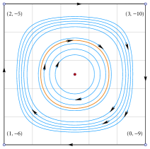
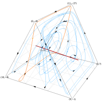
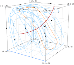
Figure 2. The evolution of (EW) in three randomly generated harmonic games with random initial conditions (left: $2\times 2$; middle: $3\times 2$; right: $2\times 2\times 2$). In all cases, the dynamics are Poincaré recurrent and cycle the game’s Nash equilibria (depicted in red). None of these games is zero-sum; the left and right games are strategically equivalent to a ZSG, while the middle is not – cf. Remark D.2. For visual clarity, we have highlighted a randomly selected orbit in each case, and the arrows indicate the direction in which orbits are traversed. In Section E.2 we include a series of trajectories of (EW)/(RD) for a convex combination of potential and a harmonic game, showing how Poincaré recurrence breaks down as the relative magnitude of the potential component increases.

A concrete consequence of the above is that, in view of Theorem 3, the trajectories of (EW) in incrompressible games are constrained to move on the level sets of a certain function. In fact, as we show in Section D.3, this function is convex, so its level sets are concentric topological spheres (as boundaries of convex sets, namely the function’s sublevel sets). In turn, this means that the phase space of the dynamics foliates into an ensemble of spheres, each of which constrains the evolution of (EW). In a certain sense, this is the closest that one can get to proving periodic behavior in general dynamics – and, in fact, by the Poincaré-Bendixson theorem, it is easy to see that the dynamics are periodic when (RD) has effective dimension $2$ or $3$ (so in the case of $2\times 2$, $2\times 3$ and $2\times 2\times 2$ games, cf. Fig. 2).

This brings us to our final result on the long-run behavior of the dynamics (EW) / (RD): Even when periodicity fails, it only fails by an arbitrarily small amount.

Theorem 4.

If $\Gamma$ is harmonic, the dynamics (EW) / (RD) are Poincaré recurrent. Specifically, for almost every initialization $x(0)\in\mathcal{X}^{\circ}$, the induced trajectory $x(t)$ returns arbitrarily close to $x(0)$ infinitely often: there exists an increasing sequence of times $t_{n}\uparrow\infty$ such that $x(t_{n})\to x(0)$.

Theorem 4 (which we prove in Appendix D) shows that the behavior of (EW)/(RD) in harmonic games is orthogonal to their behavior in potential games: in the latter, every orbit eventually converges to Nash equilibrium; in the former, the system’s orbits cycle back in an almost-periodic manner to (a neighborhood of) their starting points infinitely often (cf. Fig. 2). This provides a partial negative answer to an open question of Candogan et al. [14] regarding the convergence of the replicator dynamics in harmonic games, and shows that potential and harmonic games are orthogonal to each other also in the sense of learning.

6. Concluding remarks

We find the equivalence between harmonic and incompressible games particularly intriguing as it links four otherwise distinct and independent notions: (it n) a standard class of game-theoretic learning schemes (which lead to no-regret, so players become more efficient over time); (it n) the existence of anti-aligned incentives (encoded by the notion of a harmonic game); and, through the surprising property of volume preservation, (it n) the existence of a constant of motion and (it n) Poincaré recurrence (the prototypical manifestation of non-convergent, quasi-periodic behavior). Theorem 4 in particular shows that the interplay between these notions is significantly more intricate than what the strong no-regret properties of (EW) might suggest: in harmonic games, the players’ long-run behavior under the dynamics of exponential / multiplicative weights is Poincaré recurrent and fails to converge, even though the empirical distribution of play converges to the game’s set of coarse correlated equilibria.

Under this light, the decomposition of a game into a potential and a harmonic/incompressible component is strongly reminiscent of Conley’s decomposition theorem [21] which states that any dynamical system can be decomposed into an attracting, convergent part, and a chain-recurrent part. Of course, Conley’s theorem concerns a decomposition of the game’s state space, not the flow itself; nonetheless, this alignment between the dynamic and strategic components of a game hints at a much deeper connection which opens up many directions for further research.

One such direction concerns the general class of follow-the-regularized-leader (FTRL) dynamics [76, 77], of which (EW)/(RD) is a special case: concretely, we conjecture here that Poincaré recurrence holds for harmonic games in the entire class of FTRL dynamics. While close in spirit, the techniques presented in this paper do not extend to the class of FTRL dynamics because the analogue of Theorem 2 fails to hold for dynamics other than (EW)/(RD), so there is no longer a clear link between incompressibility and harmonicity. We leave this question open for the future.

Appendix A Basic facts and definitions from Riemannian geometry

Riemannian geometry, a cornerstone of differential geometry, provides a powerful framework for analyzing spaces endowed with a metric structure. At its core lies the notion of a Riemannian manifold, a smooth manifold endowed with a smoothly varying inner product structure on its tangent spaces. This structure allows for the definition of gradient directions of smooth functions, lengths of curves, angles between tangent vectors, and various notions of curvature, enabling the study and analysis of geometric properties of the manifold, and of dynamical systems defined thereon. In what follows, we provide a quick dictionary of some of the basic notions that we use throughout our paper.

A.1. Riemannian manifolds

A smooth manifold $\mathcal{M}$ of dimension $n$ is a Hausdorff, second countable topological space equipped with a collection of local charts $(U_{\alpha},\pi_{\alpha})$, where each $U_{\alpha}$ is an open subset of $M$ and each $\pi_{\alpha}:U_{\alpha}\rightarrow\mathbb{R}^{n}$ is a homeomorphism onto an open subset of $\mathbb{R}^{n}$. Points in the co-domain of each local chart are called local coordinates.

The tangent space $\operatorname{T}_{x}\mathcal{M}$ of a smooth manifold $\mathcal{M}$ at a point $x\in\mathcal{M}$ is the vector space of all derivations on the space of smooth functions defined on an open neighborhood of $x$; the dimension of $\operatorname{T}_{x}\mathcal{M}$ is the same as the dimension of $\mathcal{M}$.

Intuitively, a smooth manifold can be thought of as a topological space that locally resembles $\mathbb{R}^{n}$; typical example of smooth manifolds include smooth surfaces in the Euclidean space. Building on this intuition, the tangent space $\operatorname{T}_{x}\mathcal{M}$ of $\mathcal{M}$ a can be thought of as the space of all possible “directions” or “velocities” one can move in from the point $x$ without leaving the surface. For instance, if $\mathcal{M}$ is the Earth’s surface, $\operatorname{T}_{x}\mathcal{M}$ at a point $x$ would be the plane including vectors representing north, south, east, west – but not upwards.

Remark A.1.

Another fundamental example of smooth manifold is the Euclidean space $\mathbb{R}^{n}$ itself, with the identity map as a chart. Its tangent space at any point $x$ is an $n$-dimensional vector space, hence isomorphic to $\mathbb{R}^{n}$; in the following we will identify the tangent space $\operatorname{T}_{x}\mathbb{R}^{n}$ with $\mathbb{R}^{n}$ itself. $\diamond$

A Riemannian manifold $(\mathcal{M},g)$ is a smooth manifold $\mathcal{M}$ together with a smoothly varying positive definite symmetric bilinear form $g_{x}:\operatorname{T}_{x}\mathcal{M}\times\operatorname{T}_{x}\mathcal{M}\rightarrow\mathbb{R}$ defined on each tangent space $\operatorname{T}_{x}\mathcal{M}$ with $x\in\mathcal{M}$. This form, called the Riemannian metric, assigns to each pair of tangent vectors $z,z^{\prime}$ at a point $x$ a real number $g_{x}(z,z^{\prime})$, satisfying:

1. Smoothness: The map $x\mapsto g_{x}$ is smooth.

2. Positive definiteness: For all $x\in\mathcal{M}$ and $z\in\operatorname{T}_{x}\mathcal{M}$, $g_{x}(z,z)\geq 0$ with equality iff $z=0$.

3. Symmetry: For all $x\in\mathcal{M}$ and $z,z^{\prime}\in\operatorname{T}_{x}\mathcal{M}$, $g_{x}(z,z^{\prime})=g_{x}(z^{\prime},z)$.

Throughout this work use equivalently the notations $g_{x}(z,z^{\prime})\equiv\langle z,z^{\prime}\rangle_{x}\equiv z^{T}\cdot g_{x}\cdot z$ for all $z,z^{\prime}\in\operatorname{T}_{x}\mathcal{M}$, where in the third expression $g_{x}$ is a $\dim\mathcal{M}\times\dim\mathcal{M}$-dimensional matrix and $\cdot$ denotes matrix multiplication.

Finally, a vector field $X$ on $\mathcal{M}$ is a smooth map $x\mapsto X(x)\in\operatorname{T}_{x}\mathcal{M}$ that for all points $x$ on the manifold gives a vector $z=X(x)$ in the tangent space to $\mathcal{M}$ at $x$. A vector field $X$ on $\mathcal{M}$ can be written locally as a linear combination $X=\sum_{a=1}^{\dim\mathcal{M}}X^{a}e_{a}$, where $X^{a}\colon\mathcal{M}\to\mathbb{R}$ is a smooth function on the manifold and $e_{a}$ is a basis vector field, i.e., $e_{a}(x)$ is the $a$-th element in a basis of $\operatorname{T}_{x}\mathcal{M}$, for all $x\in\mathcal{M}$ and all $a=1,\dots,\dim\mathcal{M}$. An ordered collection $\{e_{a}\}_{a=1,\dots,\dim\mathcal{M}}$ of such basis vector fields is called frame bundle.

A.2. Riemannian gradients

Given a Riemannian manifold $(\mathcal{M},g)$ and a smooth function $f\colon\mathcal{M}\to\mathbb{R}$, a Riemannian metric allows to define a special vector field on $\mathcal{M}$:

Definition 2.

The gradient of $f$ is the vector field $\operatorname{grad}f$ on $\mathcal{M}$ defined by

$$\langle\operatorname{grad}f(x),z\rangle_{x}=\kern 0.0pt\partial\mkern-1.0mu{}f(x;z)\in\mathbb{R}\,,$$ (A.1)

for all points $x\in\mathcal{M}$ and all tangent vectors $z\in\operatorname{T}_{x}\mathcal{M}$.

The components of $\operatorname{grad}f$ can be expressed in any local chart as follows: let $X=e_{a}$ be a basis vector field with $a\in\{1,\dots,\dim\mathcal{M}\}$, and denote by $[df(x)]_{a}\coloneqq\kern 0.0pt\partial\mkern-1.0mu{}f(x;e_{a}(x))$ the directional derivative of $f$ at $x$ in the direction of $e_{a}(x)$.

Lemma A.1 (Components of gradient field).

For all $x\in\mathcal{M}$, the components of $\operatorname{grad}f$ are given by the matrix multiplication between the inverse matrix of the metric $g^{-1}$, and the array of basis directional derivatives $df$:

$$\operatorname{grad}f(x)=g^{-1}(x)df(x)\,.$$ (A.2)

Proof.

Write $G_{a}(x)\coloneqq[\operatorname{grad}f(x)]_{a}$. By symmetry of $g$,

$$\langle\operatorname{grad}f(x),e_{a}(x)\rangle_{x}=\sum_{b,c=1}^{\dim{\mathcal{M}}}g_{bc}(x)\,G_{b}(x)\,\delta_{ac}=\sum_{b=1}^{\dim{\mathcal{M}}}g_{ba}(x)\,G_{b}(x)=[g(x)G(x)]_{a}\,.$$

By definition of gradient this expression is equal to $[df(x)]_{a}$, so we get the matrix equation $g(x)G(x)=df(x)$ for all $x\in\mathcal{M}$. Since $g(x)$ is positive-definite for all $x\in\mathcal{M}$ we can multiply from the left both sides of this equations by the inverse matrix $g^{-1}(x)$ to get (A.2). ∎

Remark A.2 (Euclidean vs. non-Euclidean gradient).

The Euclidean metric in $\mathbb{R}^{n}$ is represented by the identity matrix $g_{ab}(x)=\delta_{ab}$, from which the familiar result that the gradient of a function is the array of basis directional derivatives, or differential, of $f$: $\operatorname{grad}f(x)=[\partial f(x;e_{a})]_{a=1}^{n}=df(x)$. In a non-Euclidean setting, the difference between the gradient and the differential of a function is given by the (inverse) metric tensor. $\diamond$

Gradients give directions of maximal rate of change

Given a smooth function $f\colon\mathcal{M}\to\mathbb{R}$ on a Riemannian manifold $(\mathcal{M},g)$, the gradient of $f$ at $x$ gives the direction of maximal rate of change of $f$ at $x$; we make this precise with the following lemma.

Lemma A.2.

On a Riemannian manifold $(\mathcal{M},g)$ let $Z_{x}\subset\operatorname{T}_{x}\mathcal{M}\coloneqq\{z\in\operatorname{T}_{x}\mathcal{M}:\lVert z\rVert_{x}=1\}$ be the set of directions at $x$, i.e., the set of tangent vectors at $x$ of unitary norm, where $\lVert z\rVert_{x}\coloneqq\sqrt{\langle z,z\rangle_{x}}$ is the the norm induced by the Riemannian inner product. Then for all smooth functions $f\colon\mathcal{M}\to\mathbb{R}$ and for all $x\in\mathcal{M}$,

$$\frac{\operatorname{grad}f(x)}{\lVert\operatorname{grad}f(x)\rVert_{x}}=\operatorname*{arg\,max}_{z\in Z_{x}}\{\partial f(x;z)\}\,.$$ (A.3)

Proof.

By definition of gradient, $\partial f(x;z)=\langle\operatorname{grad}f(x),z\rangle_{x}$. By Cauchy-Schwarz inequality, we have $\lvert\langle z,z^{\prime}\rangle_{x}\rvert\leq\lVert z\rVert_{x}\,\lVert z^{\prime}\rVert_{x}$ for all $z,z^{\prime}\in\operatorname{T}_{x}\mathcal{M}$ with equality iff $z\propto z^{\prime}$, thus $\partial f(x;z)$ is maximized in the direction $z\propto\operatorname{grad}f(x)$. ∎

A.3. Riemannian divergence

In vector calculus, the divergence is a differential operator mapping a vector field $X$ to a function:

$$\operatorname{div}{X}=\sum_{a=1}^{\dim\mathcal{M}}\frac{\partial}{\partial x_{a}}X^{a}\quad\text{[Euclidean]}\,.$$ (A.4)

This operator captures how much the field is locally spreading out or converging at a given point: loosely speaking, if the divergence is positive in the neighborhood of a point, the vector field is locally spreading out (e.g., the outward-radial field $X(x,y)=(x,y)$); if it is negative, the vector field is locally converging (e.g., the inward-radial field $X(x,y)=(-x,-y)$); and if it is zero, the field is neither locally spreading out nor converging (e.g., the hyperbolic field $X(x,y)=(x,-y)$ or the spherical field $X(x,y)=(y,-x)$).

Let $\mathfrak{X}$ and $\mathfrak{F}$ denote respectively the space of vector fields and smooth functions on a Riemannian manifold $(\mathcal{M},g)$. To generalize the divergence operator to this setting one must take into account how the volume element of the metric $g$ changes from point to point, and this in turn depends on the determinant $\det{g}$ – cf. Eq. A.11. With this idea in mind, we give the following generalization of the Euclidean divergence operator to a Riemannian setting [53, 44, 54].

Definition 3.

The divergence operator $\operatorname{div}\colon\mathfrak{X}\to\mathfrak{F}$ on a Riemannian manifold $(\mathcal{M},g)$ is defined by

$$\operatorname{div}{X}=\frac{1}{\sqrt{D}}\sum_{a=1}^{\dim\mathcal{M}}\frac{\partial}{\partial x_{a}}\left(\sqrt{D}X^{a}\right)\quad\text{for all }X\in\mathfrak{X}\,,$$ (A.5)

where $D\coloneqq\det{g}$. $\diamond$

Remark A.3.

If $(\mathcal{M},g)$ is the standard Euclidean space equipped with the Euclidean metric then the constant term $\sqrt{D}$ is not affected by the partial derivatives and cancels out with $(\sqrt{D})^{-1}$, giving back the familiar Eq. A.4. $\diamond$

Note that Eq. A.5 can be rewritten by product rule as

$$\operatorname{div}{X}=\sum_{a=1}^{\dim\mathcal{M}}\left(\frac{\partial_{a}\sqrt{D}}{\sqrt{D}}\right)X^{a}+\sum_{a=1}^{\dim\mathcal{M}}\partial_{a}X^{a}\,,$$ (A.6)

where $\partial_{a}$ is a shorthand for $\frac{\partial}{\partial x_{a}}$.

Example A.1 (Divergence on the sphere).

The determinant of the Euclidean metric in $\mathbb{R}^{3}$ induced on the unit sphere in standard spherical coordinates fulfills $\sqrt{\det{g}}=\sin\theta$, so by Eq. A.6 the divergence of the vector field $X(\theta,\phi)=(X^{\theta},X^{\phi})$ is

$$\operatorname{div}{X}=\partial_{\theta}X^{\theta}+\partial_{\phi}X^{\phi}+\frac{X^{\theta}}{\tan{\theta}}\,.$$

In particular the divergence of a longitudinal vector field $X=(1,0)$ is $\frac{1}{\tan\theta}$, which diverges to infinity a the north pole, is zero at the equator, and diverges to minus infinity at the south pole. This captures the fact that a small set of initial conditions starting close to the north pole and evolving along flow of $X$ quickly expands moving towards the equator; the rate of expansion decreases until the equator is crossed, after which the flow lines converge at increasingly higher rate towards the south pole.

Conversely, the divergence of a latitudinal vector field $X=(0,1)$ is $0$, capturing the fact that the volume of a small set of initial conditions remains constant along the flowlines parallel to the equator. $\diamond$

Riemannian divergence on product manifold

In this section we show that the divergence operators on two Riemannian manifolds naturally induce a divergence operator on the product manifold.

Let $(\mathcal{M},g_{\mathcal{M}})$ and $(\mathcal{M}^{\prime},g_{\mathcal{M}^{\prime}})$ be Riemannian manifolds with coordinates $x$ and $x^{\prime}$ respectively, with $g_{\mathcal{M}}$ represented by the matrix $(g_{\mathcal{M}})_{ij}$ for $i,j=1,\dots,\dim\mathcal{M}$, and $g_{\mathcal{M}^{\prime}}$ represented by the matrix $(g_{\mathcal{M}^{\prime}})_{hk}$ for $h,k=1,\dots,\dim\mathcal{M}^{\prime}$. Consider the product manifold $P=\mathcal{M}\times\mathcal{M}^{\prime}$ with $\dim{P}=\dim{\mathcal{M}}+\dim{\mathcal{M}^{\prime}}$, coordinates $(x,x^{\prime})$, and metric $g(x,x^{\prime})\coloneqq g_{\mathcal{M}}(x)+g_{\mathcal{M}^{\prime}}(x^{\prime})$. The matrix representing the metric $g$ is the block diagonal matrix with the matrices of $g_{\mathcal{M}}$ and $g_{\mathcal{M}^{\prime}}$ on the diagonal, so $\det{g}=\det{g_{\mathcal{M}}}\det{g_{\mathcal{M}^{\prime}}}$. In the following we denote $D\coloneqq\det{g}=D_{\mathcal{M}}D_{\mathcal{M}^{\prime}}$.

A vector field $X$ on $\mathcal{M}$ locally written as $X(x)=\sum\nolimits_{i=1}^{\dim\mathcal{M}}X^{i}(x)e_{x_{i}}$ can be naturally seen as a vector field $X$ on $P$, given by $X(x,x^{\prime})=\sum\nolimits_{A=1}^{\dim{P}}X^{A}(x,x^{\prime})e_{A}=\sum\nolimits_{i=1}^{\dim{\mathcal{M}}}X^{i}(x)e_{x_{i}}+\sum\nolimits_{j=1}^{\dim{\mathcal{M}^{\prime}}}0\,e_{x^{\prime}_{j}}$. With this identification in mind, two vector fields $X$ on $\mathcal{M}$ and $X^{\prime}$ on $\mathcal{M}^{\prime}$ naturally give a vector field $Z$ on $P$ by $Z(x,x^{\prime})\coloneqq X(x)+X^{\prime}(x^{\prime})=\sum\nolimits_{i=1}^{\dim\mathcal{M}}X^{i}(x)e_{x_{i}}+\sum\nolimits_{j=1}^{\dim\mathcal{M}^{\prime}}X^{\prime j}(x^{\prime})e_{x^{\prime}_{j}}$.

Lemma A.3 (The divergence operator does not mix coordinates).

Let $X$ be a vector field on a Riemannian manifold $(\mathcal{M},g)$ and $X^{\prime}$ a vector field on a Riemannian manifold $(\mathcal{M}^{\prime},g^{\prime})$. Then the vector field $Z=X+X^{\prime}$ on the product manifold $(P=\mathcal{M}\times\mathcal{M}^{\prime},g=g_{\mathcal{M}}+g_{\mathcal{M}^{\prime}})$ fulfills

$$\operatorname{div}_{g}{Z}=\operatorname{div}_{g_{\mathcal{M}}}{X}+\operatorname{div}_{g_{\mathcal{M}^{\prime}}}{X^{\prime}}\,.$$ (A.7)

Proof.

The $\operatorname{div}{}$ operator acts linearly on vector fields [53], so

$$\operatorname{div}_{g}{Z}=\operatorname{div}_{g}{X}+\operatorname{div}_{g}{X^{\prime}}\quad\text{by linearity of }\operatorname{div}{}\,.$$

So if we show that $\operatorname{div}_{g}{X}=\operatorname{div}_{g_{\mathcal{M}}}{X}$ we are done. This is true since the coordinates of the two manifolds remain decoupled under the Cartesian product operation, so they are acted upon only by derivatives of the corresponding type:

$$\begin{split}\operatorname{div}_{g}{X}&=\sum_{A=1}^{\dim{P}}\left(\frac{\partial_{A}\sqrt{D}}{\sqrt{D}}\right)X^{A}+\sum_{A=1}^{\dim{P}}\partial_{A}X^{A}\\ &=\sum_{i=1}^{\dim{\mathcal{M}}}\left(\frac{\partial_{x_{i}}\left(\sqrt{D_{\mathcal{M}}}\sqrt{D_{\mathcal{M}^{\prime}}}\right)}{\sqrt{D_{\mathcal{M}}}\sqrt{D_{\mathcal{M}^{\prime}}}}\right)X^{i}+\sum_{i=1}^{\dim{\mathcal{M}}}\partial_{x_{i}}X^{i}+\sum_{j=1}^{\dim{\mathcal{M}^{\prime}}}0\,.\\ \end{split}$$

Now $\partial_{x_{i}}\left(\sqrt{D_{\mathcal{M}}}\sqrt{D_{\mathcal{M}^{\prime}}}\right)=\partial_{x_{i}}\left(\sqrt{D_{\mathcal{M}}}\right)\sqrt{D_{\mathcal{M}^{\prime}}}$, so the terms containing $\sqrt{D_{\mathcal{M}^{\prime}}}$ simplify:

$$\operatorname{div}_{g}{X}=\sum_{i=1}^{\dim{\mathcal{M}}}\left(\frac{\partial_{x_{i}}\left(\sqrt{D_{\mathcal{M}}}\right)}{\sqrt{D_{\mathcal{M}}}}\right)X^{i}+\sum_{i=1}^{\dim{\mathcal{M}}}\partial_{x_{i}}X^{i}=\operatorname{div}_{g_{\mathcal{M}}}{X}\,.\qed$$

A.4. Flows on manifolds

We recall here a few concepts from the theory of dynamical systems on manifolds. We refer the reader to Lee [53, Ch. 9,16] for the general theory and to Flokas et al. [26] for a concise treatment in the context of no-regret learning. For a detailed account of the theory of ordinary differential equations and deterministic dynamical systems in continuous time in the context of multipopulation evolutionary dynamics we refer the reader to the excellent introduction by Weibull [86, Ch. 6], and in particular to Section 6.6 for a general discussion on the Euclidean version of Liouville’s theorem, and to sections 5.2.2 and 5.8.2 for relevant applications.

Given a smooth vector field $X\in\mathfrak{X}$ on a smooth manifold $\mathcal{M}$, a smooth global integral curve of $X$ is a smooth curve $\gamma\colon\mathbb{R}\to\mathcal{M}$ such that $\dot{\gamma}(t)=X(\gamma(t))$ for all $t\in\mathbb{R}$. The point $\gamma(0)$ is called starting point of $\gamma$. If a smooth global integral curve $\gamma$ of $X$ with starting point $x$ exists, then it is the unique maximal solution to the initial value problem

$$\dot{\gamma}=X(\gamma),\quad\gamma(0)=x\,.$$ (IVP)

Given a smooth manifold $\mathcal{M}$, a smooth global flow on $\mathcal{M}$ is a smooth map $\theta\colon\mathbb{R}\times\mathcal{M}\to\mathcal{M}$ such that for all $t,s\in\mathbb{R}$ and $x\in\mathcal{M}$, $\theta(t,\theta(s,x))=\theta(t+s,x)$ and $\theta(0,x)=x$. Given a smooth global flow, fixing $t\in\mathbb{R}$ one can define the orbit map $\theta_{t}\colon\mathcal{M}\to\mathcal{M}$ by $\theta_{t}(x)=\theta(t,x)$; the orbit map of a smooth global flow can be shown to be a diffeomorphism of $\mathcal{M}$ onto itself with inverse $\left(\theta_{t}\right)^{-1}=\theta_{-t}$. Similarly, by fixing $x\in\mathcal{M}$ one can define the curve $\theta^{x}\colon\mathbb{R}\to\mathcal{M}$ by $\theta^{x}(t)=\theta(t,x)$.

Given a smooth global flow $\theta$ and a smooth vector field $X\in\mathfrak{X}$ on a smooth manifold $\mathcal{M}$, we say that $\theta$ is the flow of $X$ if $X\left(\theta^{x}(t)\right)=\dot{\theta^{x}}(t)$ for all $t\in\mathbb{R}$ and $x\in\mathcal{M}$. If $X$ admits a global flow, then $\theta^{x}\colon\mathbb{R}\to\mathcal{M}$ is an integral curve of $X$ with starting point $x$, hence a solution to the initial value problem (IVP) – equivalently, the orbit map $\theta_{t}\colon\mathcal{M}\to\mathcal{M}$ maps any initial condition $x\in\mathcal{M}$ to the point $\gamma(t)$, where $\gamma$ is the maximal solution to the initial value problem (IVP).

A vector field may not always admit a global flow, since it may not always be the case that every integral curve is defined for all time. The Fundamental Theorem of Flows [53, Th. 9.12] asserts that every smooth vector field on a smooth manifold determines a unique local maximal smooth flow; the proof is an application of the existence, uniqueness, and smoothness theorem for solutions of ordinary differential equations. For the scope of this work note that the trajectories of (RD) on $\mathcal{X}^{\circ}$ are defined for all $t\in\mathbb{R}$, so the replicator vector field $v^{\sharp}$ defines a smooth global flow on $\mathcal{X}^{\circ}$.

Next, we look at the relation between the Riemannian divergence of a vector field defined in Section A.3, and the volume of a set of initial conditions evolving along the flow of such vector field. We warm up in an Euclidean setting, before moving to a Riemannian one.

The Euclidean Liouville’s theorem

Consider a vector field $X\in\mathfrak{X}$ on $\mathcal{M}=\mathbb{R}^{n}$ that admits a global flow $\theta\colon\mathbb{R}\times\mathbb{R}^{n}\to\mathbb{R}^{n}$. For any open set $\mathcal{U}\subseteq\mathbb{R}^{n}$ and any $t\in\mathbb{R}$ denote by $\mathcal{U}_{t}$ the image of $\mathcal{U}$ under the orbit map $\theta_{t}\colon\mathbb{R}^{n}\to\mathbb{R}^{n}$:

$$\mathcal{U}_{t}\coloneqq\theta_{t}(\mathcal{U})=\{\theta_{t}(x):x\in\mathcal{U}\}\subseteq\mathbb{R}^{n}\,.$$ (A.8)

Note that $\mathcal{U}_{t=0}=\mathcal{U}$, since the orbit map $\theta_{0}$ is the identity map on $\mathbb{R}^{n}$.

A fundamental result of classical mechanics known as Liouville’s theorem [5] relates the Euclidean divergence (A.4) of the vector field $X$, which is a function $\operatorname{div}{X}\colon\mathbb{R}^{n}\to\mathbb{R}$, with the Euclidean volume of an open set of initial conditions evolving along the flow of $X$:

Theorem (Euclidean Liouville’s theorem).

Given a smooth vector field $X$ in $\mathbb{R}^{n}$ and an open set $\mathcal{U}\subseteq\mathbb{R}^{n}$,

$$\frac{d}{dt}\operatorname{vol}(\mathcal{U}_{t})=\int_{\mathcal{U}_{t}}\operatorname{div}{X}dx\,,$$ (A.9)

for all $t\in\mathbb{R}$ such that the flow of $X$ is defined.

Proof.

See e.g., Arnold [5, Ch. 3]. ∎

If a map $\phi\colon\mathbb{R}^{n}\to\mathbb{R}^{n}$ fulfills $\operatorname{vol}(\mathcal{U})=\operatorname{vol}(\phi\mathcal{U})$ for all open subsets $\mathcal{U}\subseteq\mathcal{M}$ we say that the map is volume-preserving. An immediate corollary of Liouville’s theorem is that the orbit maps of vector fields with zero divergence are volume-preserving:

Corollary (Conservation of Euclidean volume).

If a vector field $X$ in $\mathbb{R}^{n}$ fulfills $\operatorname{div}X=0$, then

$$\operatorname{vol}(\mathcal{U}_{t})=\operatorname{vol}(\mathcal{U})$$ (A.10)

for all open sets $\mathcal{U}\subseteq\mathbb{R}^{n}$ and all $t\in\mathbb{R}$ such that the flow of $X$ is defined.

Proof.

If $\operatorname{div}X=0$ the right hand side of Eq. A.9 vanishes, hence $\operatorname{vol}{\mathcal{U}_{t}}$ is constant whenever the flow of $X$ is defined. ∎

The Riemannian Liouville’s theorem

The constructions of the previous paragraph generalize to the more general setting of Riemannian manifolds [53, Ch. 16]. Given a smooth vector field $X\in\mathfrak{X}$ that admits a global flow $\theta$ on a Riemannian manifold $(\mathcal{M},g)$ of dimension $n$, let $\mathcal{U}_{t}=\theta_{t}(\mathcal{U})$ be the image of any open subset $\mathcal{U}\subseteq\mathcal{M}$ under the orbit map $\theta_{t}\colon\mathcal{M}\to\mathcal{M}$, as in Eq. A.8. To generalize the Euclidean Liouville’s theorem to this Riemannian setting we need the appropriate notions of divergence of a vector field and volume of an open set on a Riemannian manifold. The appropriate generalization of the divergence operator is given by Eq. A.5; the appropriate notion of volume on a Riemannian manifold is the following [53, Ch. 16]: If $\mathcal{U}$ is an open subset completely contained in the domain of a single smooth chart $(\mathcal{V},\pi)$ of $\mathcal{M}$, then its Riemannian volume is

$$\operatorname{vol}{\mathcal{U}}=\int_{\pi(\mathcal{U})}\sqrt{\det\tilde{g}(\tilde{x})}\,d\tilde{x}\,,$$ (A.11)

where $\pi\colon\mathcal{U}\to\mathbb{R}^{n}$ is an homeomorphism onto an open subset $\tilde{\mathcal{U}}\coloneqq\pi(\mathcal{U})$ of $\mathbb{R}^{n}$ mapping $x\in\mathcal{M}$ to $\tilde{x}\in\tilde{\mathcal{U}}$; and $\tilde{g}$ is the effective representation of the Riemannian metric $g$ on $\tilde{\mathcal{U}}$ (cf. Section B.4).

With these definitions at hand we can state the Riemannian version of Liouville’s theorem:

Theorem (Riemannian Liouville’s theorem).

Given a vector field $X\in\mathfrak{X}$ on a Riemannian manifold $(\mathcal{M},g)$ and an open set $\mathcal{U}\subseteq\mathcal{M}$,

$$\frac{d}{dt}\operatorname{vol}(\mathcal{U}_{t})=\int_{\pi(\mathcal{U}_{t})}\operatorname{div}{X}dx$$ (A.12)

for all $t\in\mathbb{R}$ such that the flow $\theta$ of $X$ is defined, where $\mathcal{U}_{t}=\theta_{t}(\mathcal{U})$ and $\pi_{0}$ is a chart whose domain contains $\mathcal{U}_{t}$.

Proof.

See e.g., Lee [53, Ch. 16]. ∎

As in the Euclidean case, if a map $\phi\colon\mathcal{M}\to\mathcal{M}$ fulfills $\operatorname{vol}(\mathcal{U})=\operatorname{vol}(\phi\mathcal{U})$ for all open subsets $\mathcal{U}\subseteq\mathcal{M}$ we say that the map is volume-preserving; and the orbit maps of vector fields with zero Riemannian divergence are volume-preserving.

Corollary (Conservation of Riemannian volume).

If a vector field $X\in\mathfrak{X}$ on a Riemannian manifold fulfills $\operatorname{div}X=0$ then

$$\operatorname{vol}(\mathcal{U}_{t})=\operatorname{vol}(\mathcal{U})\,,$$ (A.13)

where $\mathcal{U}_{t}=\theta_{t}(\mathcal{U})$, for all open sets $\mathcal{U}\subseteq\mathcal{M}$ and all $t\in\mathbb{R}$ such that the flow $\theta$ of $X$ is defined.

Proof.

The proof is identical to the one for the Euclidean counterpart. ∎

Poincaré recurrence

The last notion we need is that of Poincaré recurrence, a property of volume-preserving maps on sets of finite volume. We present a measure-theoretic version of Poincaré’s classical recurrence theorem, and adapt it to our Riemannian framework.

Given a measure space $(\Omega,\mu)$, we say that $(\Omega,\mu)$ is finite if $\mu(\Omega)<\infty$, and that a map $\phi\colon\Omega\to\Omega$ is measure preserving if $\mu(\phi\mathcal{U})=\mu(\mathcal{U})$ for all measurable subsets $\mathcal{U}\subseteq\Omega$. Given a finite measure that is invariant under some map one has the following theorem [10]:

Theorem (Poincaré – Measure setting).

Let $(\Omega,\mu)$ be a finite measure space, and let $\phi\colon\Omega\to\Omega$ be a measure preserving mapping. Let $\mathcal{U}$ be a measurable subset of $\Omega$. Then almost every point $x\in\mathcal{U}$ is infinitely recurrent with respect to $\mathcal{U}$, that is, the set $\{n\in\mathbb{N}:\phi^{n}x\in\mathcal{U}\}$ is infinite.

Proof.

See e.g., Bekka et al. [10, Th. 1.7]. ∎

Remark A.4.

The Riemannian volume Eq. A.11 on a Riemannian manifold $(\mathcal{M},g)$ defines a measure $\mu$ on the Borel sigma-algebra of $\mathcal{M}$ by $\mu(\mathcal{U})=\operatorname{vol}{\mathcal{U}}$, hence a Riemannian manifold is in particular a measure space [80], on which Poincaré’s theorem applies. Furthermore every Riemannian manifold is a separable metric space, so one can formulate a Riemannian version of Poincaré’s theorem: given a Riemannian manifold $(\mathcal{M},g)$ of finite volume and a volume-preserving map $\phi\colon\mathcal{M}\to\mathcal{M}$, almost every point $x\in\mathcal{M}$ is $\phi$-recurrent, that is, there is a strictly increasing sequence of integers $t_{n}\uparrow\infty$ such that $\lim_{n\to\infty}\phi^{t_{n}}x\to x$; see Bekka et al. [10, Corollary 1.8].

The tools presented in this appendix will be used in Appendix D to prove some of the main results of this paper, namely that a game is incompressible if and only if it is harmonic (via a Riemannian divergence operator); that replicator dynamics on incompressible games are volume-preserving with respect to a non-Euclidean Riemannian structure (via Liouville’s theorem); and that replicator dynamics on incompressible games exhibit Poincaré recurrence (via Poincaré’s theorem).

Appendix B Effective representation of games

Figure 3. Maps (B.1) and (B.2) between the open corner of cube $\mathcal{C}^{\circ}$ in $\mathbb{R}^{m}$ and the open simplex $\mathcal{X}^{\circ}$ in $\mathbb{R}^{m+1}$ for $m=2$. In light red are the tangent spaces $\operatorname{T}\mathcal{C}^{\circ}=\mathbb{R}^{2}$ and $\operatorname{T}\mathcal{X}^{\circ}=\mathcal{Z}$, where $\mathcal{Z}$ is the hyperplane $\mathcal{Z}=\{(x_{0},x_{1},x_{2})\in\mathbb{R}^{3}:x_{0}+x_{1}+x_{2}=0\}$. The basis vectors $\tilde{e}_{1}=(1,0)$ and $\tilde{e}_{2}=(0,1)$ of $\operatorname{T}\mathcal{C}^{\circ}$ are mapped by Eq. B.21 to the vectors $\tilde{e}_{1}=e_{1}-e_{0}=(-1,1,0)$ and $\tilde{e}_{2}=e_{2}-e_{0}=(-1,0,1)$ in $\mathcal{Z}$.

Given the finite normal form game $\Gamma=\Gamma(\mathcal{N},\mathcal{A},u)$ let $A_{i}\equiv m_{i}+1$ be the number of pure strategies of player $i\in\mathcal{N}$, and denote the set of their pure strategies as $\mathcal{A}_{i}=\{0_{i},1_{i},\dots,m_{i}\}$. Define $\tilde{\mathcal{A}}_{i}\coloneqq\{1_{i},\dots,m_{i}\}$; in the following the index $\alpha_{i}\in\mathcal{A}_{i}$ runs from $0_{i}$ to $m_{i}$, and the index $\mu_{i}\in\tilde{\mathcal{A}}_{i}$ runs from $1_{i}$ to $m_{i}$, unless otherwise specified.

Finite games in this form carry two intrinsic redundancies. First, $m_{i}$ out of the $m_{i}+1$ components of the mixed strategy $x_{i}\in\mathcal{X}_{i}$ of player $i$ are sufficient to completely specify it, since the remaining one is constrained by $\sum_{\alpha_{i}}x_{i\alpha_{i}}=1$. Second, two strategically equivalent games, albeit having different payoff functions, effectively represent the same game, since they display the same strategical and dynamical properties. For this reason it is desiderable to introduce a reduced or effective representation of a game, in which (1) the mixed strategy of each player is represented by an $m_{i}$-dimensional object, and (2) strategically equivalent games are “clearly” the same, in a sense to be made precise.

To this end consider for each player the coordinates transformation between their strategy space $\mathcal{X}_{i}=\operatorname{\operatorname{\Delta}}(\mathcal{A}_{i})=\{x_{i}\in\mathbb{R}_{+}^{m_{i}+1}:\sum_{\alpha_{i}\in\mathcal{A}_{i}}x_{i\alpha_{i}}=1\}$ and the corner of cube simplex $\mathcal{C}_{i}=\{\tilde{x}_{i}\in\mathbb{R}_{+}^{m_{i}}:\sum_{\mu_{i}\in\tilde{\mathcal{A}}_{i}}\tilde{x}_{\mu}\leq 1\}$ given by

$$\begin{aligned} \iota_{0}\colon\,&\mathcal{C}_{i}\to\mathcal{X}_{i}\\ &\tilde{x}_{i}\longmapsto x_{i}\end{aligned}\quad\text{such that}\quad\begin{cases}x_{i0_{i}}=1-\sum_{\mu_{i}=1}^{{}^{m_{i}}}\tilde{x}_{i\mu_{i}}\\ x_{i\mu_{i}}=\tilde{x}_{i\mu_{i}}\quad\text{for all }\mu_{i}\in\{1,\dots,m_{i}\}\,.\end{cases}$$ (B.1)

This map is visualized in Fig. 3 with its obvious inverse

$$\begin{aligned} \pi_{0}\colon\,&\mathcal{X}_{i}\to\mathcal{C}_{i}\\ &x_{i}\longmapsto\tilde{x}_{i}\end{aligned}\quad\text{such that}\quad\tilde{x}_{i\mu_{i}}=x_{i\mu_{i}}\quad\text{for all }\mu_{i}\in\{1,\dots,m_{i}\}\,.$$ (B.2)

This standard reduction technique goes back at least to Ritzberger & Vogelsberger [72, p. 4], and is employed in many other works [35, 59, 50, 51, 22, 13, 86, 37, 81].

In the following we consider only interior strategies by restricting $\iota_{0}$ to $\iota_{0}|_{\mathcal{C}^{\circ}_{i}}\colon\mathcal{C}^{\circ}_{i}\to\mathcal{X}^{\circ}_{i}$ (and we will denote $\iota_{0}|_{\mathcal{C}^{\circ}}$ just by $\iota_{0}$). Geometrically, the reason to consider the relative interior of the strategy space is that $\mathcal{X}^{\circ}_{i}$ is a smooth manifold of dimension $m_{i}$ with a global chart $\pi_{0}$ onto the open corner of cube $\mathcal{C}^{\circ}_{i}$, which is an open subset of $\mathbb{R}^{m_{i}}$; on the other hand, $\mathcal{X}_{i}$ is not a smooth manifold (cf. Appendix A). For a dynamical justification of the restriction to the interior of $\mathcal{X}_{i}$, cf. Eq. C.2 and the surrounding discussion.

Under the maps $\iota_{0}$ and its inverse $\pi_{0}$ the open corner of cube and the open simplex are fundamentally the same object; the corner of cube representation retains all the information existing on the simplex in a more efficient way, getting rid of the redundant degree of freedom. Thus, all the objects and structures defined on the open simplex $\mathcal{X}^{\circ}_{i}$ as a subspace of $\mathbb{R}_{++}^{m_{i}+1}$ – such as payoff functions and payoff fields, vector fields and metrics – must admit via Eqs. B.1 and B.2 an equivalent representation on the open corner of cube $\mathcal{C}^{\circ}_{i}$, that we’ll refer to interchangeably as reduced or effective. As opposed to effective, we will refer to objects defined on $\mathcal{X}^{\circ}_{i}$ as full.

In the next paragraphs we will present for each open simplex $\mathcal{X}^{\circ}_{i}$ and its corresponding open corner of cube $\mathcal{C}^{\circ}_{i}$ the effective representation of payoff functions and payoff fields, replicator dynamics, tangent vectors, and metric tensors. The end result of this reduction procedure is the effective representation of the mixed extension of a finite game $\Gamma(\mathcal{N},\mathcal{A},u)$, in which all the relevant objects are define on (the interior of) the product corner of cube $\mathcal{C}=\prod_{i\in\mathcal{N}}\mathcal{C}_{i}$, rather than on the “redundant” original strategy space $\mathcal{X}=\prod_{i\in\mathcal{N}}\mathcal{X}_{i}$.

B.1. Effective representation of payoff functions and payoff fields

Figure 4. A $(2\times 2)$ game. Left: The strategy space of each player $i\in\{1,2\}$ in a $(2\times 2)$ game is the $1$-dimensional open simplex $\mathcal{X}^{\circ}_{i}$ as a subspace of $\mathbb{R}^{2}$; the tangent space $\operatorname{T}\mathcal{X}^{\circ}_{i}$ is the line $x_{0}+x_{1}=0$. Right: The strategy space $\mathcal{X}^{\circ}_{1}\times\mathcal{X}^{\circ}_{2}$ of a $2\times 2$ game is a subset of $\mathbb{R}^{4}$, so we represent the open corner of cube $\mathcal{C}^{\circ}=\mathcal{C}^{\circ}_{1}\times\mathcal{C}^{\circ}_{2}=\{(\tilde{x}_{1},\,\tilde{x}_{2}):\tilde{x}_{1}>0,\,\tilde{x}_{2}>0,\,\tilde{x}_{1}<1,\,\tilde{x}_{2}<1\}$ as an open subset of $\mathbb{R}^{2}$. Its tangent space $\operatorname{T}\mathcal{C}^{\circ}$ is the whole $\mathbb{R}^{2}$.

The effective representation of mixed strategies is given precisely by Eq. B.2. Since payoff functions are scalar functions of these strategies, the effective representation $\tilde{u}_{i}\colon\mathcal{C}^{\circ}_{i}\to\mathbb{R}$ of the payoff function $u_{i}\colon\mathcal{X}^{\circ}_{i}\to\mathbb{R}$ is obtained as the restriction of $u_{i}$ to $\mathcal{C}^{\circ}_{i}$, i.e.,

$$\tilde{u}_{i}(\tilde{x})=u_{i}(x)$$ (B.3)

for all $i\in\mathcal{N}$, and all $\tilde{x}\in\mathcal{C}^{\circ},x\in\mathcal{X}$ related by Eq. B.1.

Just like the full payoff field is obtained differentiating the full payoff functions, the reduced payoff field is obtained differentiating the reduced payoff functions:

$$v_{i\alpha_{i}}(x)=u_{i}(\alpha_{i};x_{-i})=\frac{\partial u_{i}}{\partial x_{i\alpha_{i}}}(x)\implies\tilde{v}_{i\mu_{i}}(\tilde{x})\coloneqq\frac{\partial\tilde{u}_{i}}{\partial\tilde{x}_{i\mu_{i}}}(\tilde{x})\,.$$ (B.4)

Remark B.1 (Individual differential).

Eq. B.4 says that the components of the full (resp. reduced) payoff field $v_{i}$ (resp. $\tilde{v}_{i}$) are obtained by partial differentiation of the payoff function $u_{i}$ (resp. $\tilde{u}_{i}$) of player $i\in\mathcal{N}$ with respect to their mixed strategies $x_{i}$ (resp. $\tilde{x}_{i}$). As mentioned in Remark A.2 we refer to the array of partial derivatives of a function as differential of the function; since we are differentiating each payoff function only with respect to the variables relative to one player, we say that the full (resp. reduced ) payoff field of a player is the individual differential of the full (resp. reduced) payoff function of the player, and for each $i\in\mathcal{N}$ we write

$$v_{i}=d_{i}u_{i}\quad\text{and}\quad\tilde{v}_{i}=\tilde{d}_{i}\tilde{u}_{i}\,.$$ (B.5)

We have the following useful lemma to compute partial derivatives in effective coordinates:

Lemma B.1.

Let $f\colon\mathcal{X}^{\circ}\to\mathbb{R}$ be a differentiable function and $\tilde{f}\colon\mathcal{C}^{\circ}\to\mathbb{R}$ its effective representation. Then

$$\frac{\partial}{\partial\tilde{x}_{i\mu_{i}}}\tilde{f}(\tilde{x})=\left(\frac{\partial}{x_{i\mu_{i}}}-\frac{\partial}{x_{i0_{i}}}\right)f(x)\,,$$ (B.6)

for all $i\in\mathcal{N},\mu_{i}\in\tilde{\mathcal{A}}_{i}$, and all $x\in\mathcal{X}^{\circ}$ and $\tilde{x}\in\mathcal{C}^{\circ}$ related by Eq. B.1.

Proof.

Fix $i\in\mathcal{N}$ and $\mu_{i}\in\tilde{\mathcal{A}}_{i}$. By the chain rule, $\frac{\partial}{\partial\tilde{x}_{i\mu_{i}}}\tilde{f}(\tilde{x})=\sum_{j\in\mathcal{N}}\sum_{\alpha_{j}=0_{j}}^{m_{j}}\frac{\partial x_{j\alpha_{j}}}{\partial\tilde{x}_{i\mu_{i}}}\frac{\partial}{\partial{x_{j\alpha_{j}}}}f(x)$. By Eq. B.1, $\frac{\partial x_{j0_{j}}}{\partial\tilde{x}_{i\mu_{i}}}=-\delta_{ij}$ and $\frac{\partial x_{j\nu_{j}}}{\partial\tilde{x}_{i\mu_{i}}}=\delta_{ij}\delta_{\mu_{i}\nu_{i}}$ for all $\nu_{j}\in\{1_{j},\dots,m_{j}\}$, and we conclude expanding the sum and substituting. ∎

Applying the previous lemma to Eq. B.4 we get the reduced expression of the payoff field:

$$\tilde{v}_{i\mu_{i}}(\tilde{x})=v_{i\mu_{i}}(x)-v_{i0_{i}}(x)\,,$$ (B.7)

with $x=\iota_{0}(\tilde{x})$ for all $\tilde{x}\in\mathcal{C}^{\circ}$ and all $i\in\mathcal{N},\,\mu_{i}=1_{i},\dotsc,m_{i}$, in agreement with Eq. 23 in the main text. The first order version of this equation gives an important relation between the Jacobian matrices of the full and reduced effective fields:

Lemma B.2.

The components of the Jacobian matrix of the effective payoff field are given by

$$\frac{\partial\tilde{v}_{i\nu_{i}}}{\partial\tilde{x}_{j\mu_{j}}}\,(\tilde{x})=\left(\frac{\partial}{\partial x_{j\mu_{j}}}-\frac{\partial}{\partial x_{j0_{j}}}\right)\,\left(v_{i\nu_{i}}-v_{i0_{i}}\right)(x)$$ (B.8)

with $x=\iota_{0}(\tilde{x})$ for all $\tilde{x}\in\mathcal{C}^{\circ}$, $i,j\in\mathcal{N}$, $\nu_{i}\in\{1,\dots,m_{i}\}$ and $\mu_{j}\in\{1,\dots,m_{j}\}$ .

Proof.

Immediate by Lemma B.1 and Eq. B.7. ∎

Next is a simple but important property of payoff fields:

Lemma B.3.

For every player $i\in\mathcal{N}$ and for every pure strategy $\alpha_{i}\in\mathcal{A}_{i}$, the component $v_{i\alpha_{i}}$ of the payoff field $v$ does not depend on the mixed strategy of player $i$:

$$\frac{\partial v_{i\alpha_{i}}}{\partial x_{i\beta_{i}}}\equiv 0$$ (B.9)

for all players $i\in\mathcal{N}$ and all $\alpha_{i},\beta_{i}\in\mathcal{A}_{i}$. Analogously, for the reduced payoff field,

$$\frac{\partial\tilde{v}_{i\mu_{i}}}{\partial\tilde{x}_{i\nu_{i}}}\equiv 0$$ (B.10)

for all players $i\in\mathcal{N}$ and all $\mu_{i},\nu_{i}\in\tilde{\mathcal{A}}_{i}$.

Proof.

The first statement is immediate by the fact that $v_{i\alpha_{i}}(x)$ is the partial derivative with respect to $x_{i\alpha_{i}}$ of the multilinear function $u_{i}(x)$; the second follows from Lemma B.2. ∎

This property will be crucial in the proof of Proposition D.1 in Appendix D.

Example B.1 ($2\times 2$ game – Effective payoff ).

Consider a $2\times 2$ game with $\mathcal{A}_{1}=\mathcal{A}_{2}=\{0,1\}$ and $\tilde{\mathcal{A}}_{1}=\tilde{\mathcal{A}}_{2}=\{1\}$. The mixed strategies in full and effective representations are respectively

$$x =\big{(}({x_{1,0}},{x_{1,1}}),({x_{2,0}},{x_{2,1}})\big{)}\in\mathcal{X}_{1}\times\mathcal{X}_{2}$$ (B.11a)

$$\tilde{x} =({\tilde{x}_{1,1}},{\tilde{x}_{2,1}})\equiv(\tilde{x}_{1},\tilde{x}_{2})\in\mathcal{C}_{1}\times\mathcal{C}_{2}\,,$$ (B.11b)

where in the second line we drop an index since $\tilde{\mathcal{A}}_{i}$ is a singleton; cf. Fig. 4. The full and effective payoff functions are

$$u_{i}(x) ={x_{1,0}}\,{x_{2,0}}\,u_{i}(0,0)+{x_{1,0}}\,{x_{2,1}}\,u_{i}(0,1)+{x_{1,1}}\,{x_{2,0}}\,u_{i}(1,0)+{x_{1,1}}\,{x_{2,1}}\,u_{i}(1,1)$$

$$\tilde{u}_{i}(\tilde{x}) =\tilde{x}_{1}\tilde{x}_{2}\big{[}u_{i}(0,0)-u_{i}(0,1)-u_{i}(1,0)+u_{i}(1,1)\big{]}+\tilde{x}_{1}\big{[}-u_{i}(0,0)+u_{i}(1,0)\big{]}$$

$$\quad+\tilde{x}_{2}\big{[}-u_{i}(0,0)+u_{i}(0,1)\big{]}+u_{i}(0,0)\,.$$ (B.12a)

Note that the full payoffs are polynomials of degree $2$ with each term of the same degree, while the reduced payoffs are polynomials of degree $2$ with terms of all possible degrees.

The two full payoff fields, with two components each, are

$$v_{1}(x)=\begin{pmatrix}{x_{2,0}}\,u_{1}(0,0)+{x_{2,1}}\,u_{1}(0,1)\\ {x_{2,0}}\,u_{1}(1,0)+{x_{2,1}}\,u_{1}(1,1)\end{pmatrix}\quad\quad v_{2}(x)=\begin{pmatrix}{x_{1,0}}\,u_{2}(0,0)+{x_{1,1}}\,u_{2}(1,0)\\ {x_{1,0}}\,u_{2}(0,1)+{x_{1,1}}\,u_{2}(1,1)\end{pmatrix}\,,$$ (B.13)

whereas the two reduced payoff fields, with one component each, are

$$\tilde{v}_{1}(\tilde{x})=\tilde{x}_{2}\big{[}u_{1}(0,0)-u_{1}(0,1)-u_{1}(1,0)+u_{1}(1,1)\big{]}-u_{1}(0,0)+u_{1}(1,0)$$ (B.14a)

$$\tilde{v}_{2}(\tilde{x})=\tilde{x}_{1}\big{[}u_{2}(0,0)-u_{2}(0,1)-u_{2}(1,0)+u_{2}(1,1)\big{]}-u_{2}(0,0)+u_{2}(0,1)\,.$$ (B.14b)

Note that $v_{i}(x)$ does not depend on $x_{i}$, and $\tilde{v}_{i}(\tilde{x})$ does not depend on $\tilde{x}_{i}$, as expected by Lemma B.3. $\diamond$

Effective payoff field and strategical equivalence

The expression for the effective payoff field can be used to show that two games are strategically equivalent if and only if they are described by the same effective payoff field. Before making this precise, we give here a simple but powerful lemma that we will use often in the following:

Lemma B.4 (Vanishing of multilinear extension).

Given a finite game $\Gamma=\Gamma(\mathcal{N},\mathcal{A},u)$ let $F\colon\mathcal{A}\to\mathbb{R}$ be a real function of pure strategy profiles and $\bar{F}\colon\mathcal{X}\to\mathbb{R}$ its multilinear extension, i.e.,

$$\bar{F}(x)=\operatorname{\mathbb{E}}_{#1}[F(\alpha)]=\sum_{\alpha\in\mathcal{A}}F(\alpha)\prod_{i\in\mathcal{N}}x_{i\alpha_{i}}\equiv\sum_{\alpha\in\mathcal{A}}F(\alpha)\,x_{\alpha}$$ (B.15)

Then $F(\alpha)=0$ for all $\alpha\in\mathcal{A}$ if and only if $\bar{F}(x)=0$ for all $x\in\mathcal{X}$.

Proof.

If $F(\alpha)=0$ for all $\alpha\in\mathcal{A}$ the conclusion is immediate. Conversely, assume that $\bar{F}(x)=0$ for all $x\in\mathcal{X}$. In particular, for any $\alpha\in\mathcal{A}$, this holds true for the mixed strategy $x_{i\beta_{i}}=\delta_{\alpha_{i}\beta_{i}}$ in which each player $i$ assigns all weight to $\alpha_{i}$, i.e., $0=\bar{F}(x)=\sum_{\beta\in\mathcal{A}}F(\beta)\prod_{i\in\mathcal{N}}\delta_{\alpha_{i}\beta_{i}}=F(\alpha)$. ∎

We now move on to show that two games are strategically equivalent if and only if they are described by the same effective payoff field. Recall from Eq. 3 in the main text that two finite games $\Gamma(\mathcal{N},\mathcal{A},u)$ and $\Gamma^{\prime}(\mathcal{N},\mathcal{A},u^{\prime})$ are strategically equivalent if

$$u^{\prime}_{i}(\beta_{i};\alpha_{-i})-u^{\prime}_{i}(\alpha_{i};\alpha_{-i})=u_{i}(\beta_{i};\alpha_{-i})-u_{i}(\alpha_{i};\alpha_{-i})$$ (3)

for all $i\in\mathcal{N}$ and all $\alpha,\beta\in\mathcal{A}$. If two games $\Gamma$ and $\Gamma^{\prime}$ are strategically equivalent, we write $\Gamma\sim\Gamma^{\prime}$.

Proposition B.1.

Two finite games are strategically equivalent if and only if they have the same effective payoff field.

The proof of this result is better broken into steps.

Firstly, following Candogan et al. [14] we give the following definition and lemma:

Definition 4 (Non-strategic game).

A finite normal form game $\Gamma(\mathcal{N},\mathcal{A},k)$ is called non-strategic if all players are indifferent between all of their choices:

$$k_{i}(\beta_{i},\alpha_{-i})=k_{i}(\alpha_{i},\alpha_{-i})$$ (B.16)

for all $i\in\mathcal{N}$, all $\alpha_{-i}\in\mathcal{A}_{-i}$, and all $\alpha_{i},\beta_{i}\in\mathcal{A}_{i}$.

Lemma B.5.

Two finite games $\Gamma(\mathcal{N},\mathcal{A},u),\Gamma^{\prime}(\mathcal{N},\mathcal{A},u^{\prime})$ are strategically equivalent if and only if their difference is a non-strategic game.

Proof.

Let $\Gamma-\Gamma^{\prime}$ be non-strategic; then $k\coloneqq u^{\prime}-u$ fulfills Eq. B.16, and rearranging the terms we immediately get Eq. 3. Conversely let $\Gamma$ and $\Gamma^{\prime}$ be strategically equivalent, and set $k\coloneqq u^{\prime}-u$; again rearrange the terms in Eq. 3 to immediately conclude that $k$ fulfills Eq. B.16. ∎

Secondly, we give the following characterization of non-strategic games:

Proposition B.2.

A finite game $\Gamma(\mathcal{N},\mathcal{A},k)$ is non-strategic if and only if its effective payoff field $\tilde{v}$ vanishes identically.

Proof.

Let $\Gamma$ be non-strategic. Then its effective payoff field fulfills

$$\begin{split}\tilde{v}_{i\mu_{i}}(\tilde{x})&=v_{i\mu_{i}}(x)-v_{i0_{i}}(x)=k_{i}(\mu_{i},x_{-i})-k_{i}(0_{i},x_{-i})\\ &=\sum_{\alpha_{-i}}x_{-i\alpha_{-i}}\,\big{[}k_{i}(\mu_{i},\alpha_{-i})-k_{i}(0_{i},\alpha_{-i})\big{]}=0\end{split}$$ (B.17)

for all $\tilde{x}\in\mathcal{C}$, all $i\in\mathcal{N}$, and all $\mu_{i}\in\{1,\dots,m_{i}\}$, where the last equality holds by definition of non-strategic game.

Conversely, let the effective payoff field $\tilde{v}(\tilde{x})$ of $\Gamma$ be identically zero for all $\tilde{x}\in\mathcal{C}$. Then by Eq. B.7 all the components $v_{i\alpha_{i}}(x)=k_{i}(\alpha_{i},x_{-i})$ of the full payoff field are equal to each other, i.e., $k_{i}(\alpha_{i},x_{-i})=k_{i}(\beta_{i},x_{-i})$ for all $x\in\mathcal{X}$ and $\alpha_{i},\beta_{i}\in\mathcal{A}_{i}$, which in turn implies that $k_{i}(\alpha_{i},\alpha_{-i})=k_{i}(\beta_{i},\alpha_{-i})$ by Lemma B.4. ∎

Finally, by Lemma B.5, Proposition B.2 is equivalent to Proposition B.1:

Proof of Proposition B.1.

Given two finite games $\Gamma(\mathcal{N},\mathcal{A},u)$, $\Gamma^{\prime}(\mathcal{N},\mathcal{A},u^{\prime})$ we have the following implications:

$$\Gamma\sim\Gamma^{\prime}\iff\Gamma-\Gamma^{\prime}\text{ is non-strategic }\iff\tilde{v}-\tilde{v}^{\prime}=0\iff\tilde{v}=\tilde{v}^{\prime}$$ (B.18)

which concludes the proof. ∎

B.2. Effective representation of the replicator dynamics

We report here for ease of reference the full replicator dynamics Eqs. RD and 4.1 and its effective representation Eqs. RD₀ and 28, already derived in the main text:

$$\dot{x}_{i\alpha_{i}}=v^{\sharp}_{i\alpha_{i}}(x)=x_{i\alpha_{i}}\left[v_{i\alpha_{i}}(x)-\sum\nolimits_{\beta_{i}=0}^{m_{i}}x_{i\beta_{i}}v_{i\beta_{i}}(x)\right]\quad\text{for all }i\in\mathcal{N}\text{ and }\alpha_{i}\in\{0,\dots,m_{i}\}\,,$$ (4.1)

$$\dot{\tilde{x}}_{i\mu_{i}}=v^{\sharp}_{i\mu_{i}}(\tilde{x})=\tilde{x}_{i\mu_{i}}\left[\tilde{v}_{i\mu_{i}}(\tilde{x})-\sum\nolimits_{\nu_{i}=1}^{m_{i}}\tilde{x}_{i\nu_{i}}\tilde{v}_{i\nu_{i}}(\tilde{x})\right]\quad\text{for all }i\in\mathcal{N}\text{ and }\mu_{i}\in\{1,\dots,m_{i}\}\,.$$ (28)

Remark B.2.

We prefer the notation $v^{\sharp}_{i\mu_{i}}$ over the more correct $\tilde{v}^{\sharp}_{i\mu_{i}}$ for the effective replicator vector field for notational simplicity when there is no risk of ambiguity, and reinstate the tilde $\tilde{\cdot}$ when we want to stress the difference between the full and effective representations of the replicator field. $\diamond$

B.3. Effective representation of tangent vectors

As we saw, the map $\iota_{0}$ can be used to obtain the effective representation of points in the strategy space (i.e., mixed strategies) and of scalar functions of these points (i.e., functions of mixed strategies); the effective representation of vectors that are tangent to the strategy space requires more care.

The open corner of cube $\mathcal{C}^{\circ}_{i}$ is an open subset of $\mathbb{R}_{++}^{m_{i}}$ in its own right, so its tangent space is the whole euclidean space, that we denote by $\operatorname{T}\mathcal{C}^{\circ}_{i}\equiv\mathbb{R}^{m_{i}}$. On the other hand $\mathcal{X}^{\circ}_{i}$ is an open subset of an affine hyperplane in $\mathbb{R}_{++}^{m_{i}+1}$, and its tangent space is give by the hyperplane $\mathcal{Z}_{i}$, the linear subspace in $\mathbb{R}^{m_{i}+1}$ of vectors whose components add up to zero, cf. Lemma C.1 and Fig. 3.

A basis vector $\tilde{e}_{i\mu_{i}}$ of $\mathbb{R}^{m_{i}}$ must correspond via $\iota_{0}$ to a vector tangent to the simplex, i.e., a vector in $\mathcal{Z}_{i}$, that we want to determine. Since $\mathcal{Z}_{i}$ is a linear subspace of $\mathbb{R}^{m_{i}+1}$, it must be possible to express via $\iota_{0}$ this sought after vector as a linear combination of basis vectors $\{e_{i\alpha_{i}}\}_{\alpha_{i}\in\{0,\dots,m_{i}\}}$ of $\mathbb{R}^{m_{i}+1}$, for all $\mu_{i}\in\{1,\dots,m_{i}\}$.

The way to obtain this identification comes from an important result in differential geometry [53]: given a smooth map between two spaces such as $\iota_{0}\colon\mathcal{C}^{\circ}_{i}\to\mathcal{X}^{\circ}_{i}$, its differential induces a linear map $d\iota_{0}\colon\mathbb{R}^{m_{i}}\to\mathcal{Z}_{i}$ between the tangent spaces to the two spaces. The matrix representing this differential is the Jacobian matrix $J$ of $\iota_{0}$, so (dropping temporarily the player index $i$ for notational simplicity) a basis vector $\tilde{e}_{\mu}\equiv\tilde{e}_{i\mu_{i}}$ of $\mathbb{R}^{m}\equiv\mathbb{R}^{m_{i}}$ is mapped to the vector $d\iota_{0}(\tilde{e}_{\mu})\in\mathcal{Z}\subset\mathbb{R}^{m+1}$ of component $\left[d\iota_{0}(\tilde{e}_{\mu})\right]_{\alpha}\equiv\left[d\iota_{0}(\tilde{e}_{i\mu_{i}})\right]_{i\alpha_{i}}$ given by

$$\left[d\iota_{0}(\tilde{e}_{\mu})\right]_{\alpha}=\sum_{\nu=1}^{m}J_{\alpha\nu}[\tilde{e}_{\mu}]_{\nu}$$ (B.19)

for all $\alpha\in\{0,\dots,m\}$. Since $\tilde{e}_{\mu}$ is a basis vector its $\nu$-th component is given by the Kronecker delta $\delta_{\mu\nu}$, so

$$\begin{split}d\iota_{0}(\tilde{e}_{\mu})&=\sum_{\alpha=0}^{m}\left[d\iota_{0}(\tilde{e}_{\mu})\right]_{\alpha}\,e_{\alpha}=\sum_{\alpha=0}^{m}J_{\alpha\mu}\,e_{\alpha}=\sum_{\alpha=0}^{m}\frac{\partial x_{\alpha}}{\partial\tilde{x}_{\mu}}\,e_{\alpha}\end{split}$$ (B.20)

for all $\mu\in\{1,\dots,m\}$. Again by Eq. B.1 we have $\frac{\partial x_{0}}{\partial\tilde{x}_{\mu}}=-1$ and $\frac{\partial x_{\nu}}{\partial\tilde{x}_{\mu}}=\delta_{\mu\nu}$ for all $\mu,\nu\in\{1,\dots,m\}$, so after reinserting the player index we get $d\iota_{0}(\tilde{e}_{i\mu_{i}})=e_{i\mu_{i}}-e_{i0_{i}}$. For notational simplicity in the following we drop the differential of the $\iota_{0}$ map and denote $d\iota_{0}(\tilde{e}_{i\mu_{i}})$ just by $\tilde{e}_{i\mu_{i}}$, so that in conclusion

$$\tilde{e}_{i\mu_{i}}=e_{i\mu_{i}}-e_{i0_{i}}$$ (B.21)

for all $i\in\mathcal{N}$ and all $\mu_{i}\in\{1,\dots,m_{i}\}$; cf. Fig. 3 for a visual example.

B.4. Shahshahani metric

As discussed in Section 4, the Euclidean metric is not attuned with the dynamical properties of replicator dynamics. For this reason Shahshahani [75] introduced a metric that “[…] turns out to be surprisingly effective in clarifying the dynamics of the [replicator dynamical] system”. In this section we present this metric in its full and effective representations, along with some of its geometrical properties.

A remark on notation: we include where needed the player index $i\in\mathcal{N}$ for ease of comparison with the other sections of this work; all expressions hold true with exactly the same form if it is omitted.

Definition 5.

The Shahshahani metric on the positive orthant $\mathbb{R}_{++}^{m_{i}+1}$ is the smoothly varying positive definite symmetric bilinear form $g_{x_{i}}\colon\mathbb{R}_{++}^{m_{i}+1}\times\mathbb{R}_{++}^{m_{i}+1}\to\mathbb{R}$ represented by the $(m_{i}+1)\times(m_{i}+1)$ matrix

$$g_{i\alpha_{i}\beta_{i}}(x_{i})\coloneqq\frac{\delta_{\alpha_{i}\beta_{i}}}{x_{i\alpha_{i}}}$$ (B.22)

for all $x_{i}\in\mathbb{R}_{++}^{\mathcal{A}_{i}}$ and $\alpha_{i},\beta_{i}\in\{0,\dots,m_{i}\}$.

Effective Shahshahani metric

The components of the effective metric tensors $\tilde{g}_{\tilde{x}_{i}}$ on $\mathcal{C}^{\circ}_{i}$ are obtained by Eq. 13 as the inner product between effective tangent vectors, that by Eq. B.21 is

$$\tilde{g}_{i\mu_{i}\nu_{i}}(\tilde{x}) =\langle\tilde{e}_{i\mu_{i}},\tilde{e}_{i\nu_{i}}\rangle_{\tilde{x}}=\langle e_{i\mu_{i}}-e_{i0_{i}},e_{i\nu_{i}}-e_{i0_{i}}\rangle_{x}$$

$$=\sum_{\alpha_{i}\beta_{i}}\frac{\delta_{\alpha_{i}\beta_{i}}}{x_{i\alpha_{i}}}\,(\delta_{\alpha_{i}\mu_{i}}-\delta_{\alpha_{i}0_{i}})(\delta_{\beta_{i}\nu_{i}}-\delta_{\beta_{i}0_{i}})$$

$$=\frac{\delta_{\mu_{i}\nu_{i}}}{x_{i\mu_{i}}}-\frac{\delta_{i\mu_{i}0_{i}}}{x_{i\mu_{i}}}-\frac{\delta_{i\nu_{i}0_{i}}}{x_{i\nu_{i}}}+\frac{1}{x_{i0_{i}}}\,.$$ (B.23)

The second and third terms vanish, so in conclusion

$$\tilde{g}_{i\mu_{i}\nu_{i}}(\tilde{x}_{i})=\frac{\delta_{\mu_{i}\nu_{i}}}{\tilde{x}_{i\mu_{i}}}+\frac{1}{1-\sum_{\rho_{i}=1}^{m_{i}}\tilde{x}_{i\rho_{i}}}$$ (B.24)

for all $i\in\mathcal{N}$, all $\mu_{i},\nu_{i}\in\{1,\dots,m_{i}\}$, and all $\tilde{x}_{i}\in\mathcal{C}^{\circ}_{i}$, in agreement with Eq. 25.

Determinant of the Shahshahani metric

Since the matrix representing the full Shahshahani metric is diagonal its determinant is immediately given by

$$\det{g_{i}}(x_{i})=\frac{1}{\prod_{\alpha_{i}=0}^{m_{i}}x_{i\alpha_{i}}}\,.$$ (B.25)

The determinant of the Shahshahani metric $\tilde{g}_{i}$ in its effective representation then follows after a standard calculation based on the matrix determinant lemma, viz.

$$\det{\tilde{g}}_{i}(\tilde{x}_{i})=\frac{1}{\left(1-\sum_{\mu_{i}=1}^{m_{i}}\tilde{x}_{i\mu_{i}}\right)\prod_{\nu_{i}=1}^{m_{i}}\tilde{x}_{i\nu_{i}}}=\frac{1}{x_{i0_{i}}\prod_{\nu_{i}=1}^{m_{i}}\tilde{x}_{i\nu_{i}}}\,.$$ (B.26)

The fact that the determinant of the full and reduced metric formally agree is a particularity of the Shahshahani metric, and is in general not true for Riemannian metrics.

Shahshahani unitary spheres

As discussed in Section 4 in the main text, the Shahshahani unit sphere $\mathbb{S}_{x_{i}}\coloneqq\{z\in\mathbb{R}_{++}^{m_{i}+1}:g_{x_{i}}(z,z)=1\}$ at $x_{i}\in\mathbb{R}_{++}^{m_{i}+1}$ becomes increasingly flattened along the $x_{i\alpha_{i}}$-axis as $x_{i\alpha_{i}}\to 0$, as depicted in Fig. 1. Indeed (omitting for a second the player index $i$) the Shahshahani unit sphere at $x$,

$$\Big{\{}z\in\mathbb{R}_{++}^{m+1}\text{ such that }g_{x}(z,z)=\sum_{\alpha\beta}\frac{\delta_{\alpha\beta}}{x_{\alpha}}z_{\alpha}z_{\beta}=\sum_{\alpha}\frac{z_{\alpha}^{2}}{x_{\alpha}}=1\Big{\}}\,,$$ (B.27)

is an hyper-ellipse with the size of the $\alpha$-th axis going to zero as $x_{\alpha}\to 0$.

Remark B.3.

As discussed in Example C.1, the behavior of the Shahshahani metric as the boundary is approached, responsible for the shrinking of unit spheres describe above, is also the key feature that confines the replicator dynamics to the interior of the strategy space. $\diamond$

This concludes our (by no means exhaustive) treatment of the geometrical properties of the Shahshahani metric; for an in-depth treatment we refer the reader to Akin [2] and Shahshahani [75]. In Appendix C we turn at some of its dynamical properties and at its deep connection with the replicator dynamics; on this matter see also [37, 61, 30, 51, 65].

Appendix C Replicator dynamics as an individual Shahshahani gradient system

In this appendix we discuss the relation between the Shahshahani metric and the replicator dynamics.

Given a finite normal form game $\Gamma(\mathcal{N},\mathcal{A},u)$, the evolution of the players’ mixed strategies $x_{i}\in\mathcal{X}_{i}=\operatorname{\operatorname{\Delta}}(\mathcal{A}_{i})=\{x_{i}\in\mathbb{R}_{+}^{\mathcal{A}_{i}}:\sum_{\alpha_{i}\in\mathcal{A}_{i}}x_{i\alpha_{i}}=1\}$ under the exponential weights learning scheme evolves according to the replicator dynamical system, that is

$$\dot{x}_{i\alpha_{i}}=x_{i\alpha_{i}}[u_{i}(\alpha_{i};x_{-i})-u_{i}(x)]=x_{i\alpha_{i}}\left[v_{i\alpha_{i}}(x)-\sum\nolimits_{\beta_{i}\in\mathcal{A}_{i}}x_{i\beta_{i}}v_{i\beta_{i}}(x)\right]$$ (RD)

for all $i\in\mathcal{N}$ and $\alpha_{i}\in\mathcal{A}_{i}$. We define $v^{\sharp}_{i\alpha_{i}}(x)\coloneqq x_{i\alpha_{i}}\left[v_{i\alpha_{i}}(x)-\sum\nolimits_{\beta_{i}\in\mathcal{A}_{i}}x_{i\beta_{i}}v_{i\beta_{i}}(x)\right]$ as in Section 4.1 in the main text, and write the replicator system more compactly as

$$\dot{x}_{i}=v^{\sharp}_{i}(x)\,.$$ (C.1)

Interior and parallelism

For (C.1) to make sense $v^{\sharp}_{i}(x)$ must point in a direction parallel to $\mathcal{X}_{i}$ for all $x$ along the trajectory. The notion of “parallelism” breaks down at the boundary of $\mathcal{X}_{i}$, but for each player $i$ the interior of $\mathcal{X}_{i}$ is invariant under $v^{\sharp}_{i}$. So by restricting our attention to dynamics with initial conditions $x_{i}(t_{0})$ in the open mixed strategies space,

$$\mathcal{X}^{\circ}_{i}=\{x_{i}\in\mathbb{R}_{++}^{\mathcal{A}_{i}}:\sum_{\alpha_{i}\in\mathcal{A}_{i}}x_{i\alpha_{i}}=1\}\,,$$ (C.2)

we are sure that $x_{i}(t)\in\mathcal{X}^{\circ}_{i}$ for all times $t$ and all players, avoiding boundary issues. This means that under (RD) each pure strategy of each player has a non-zero probability to be played at all times, i.e., $x_{i\alpha_{i}}\neq 0$ for all $i\in\mathcal{N}$ and all $\alpha_{i}\in\mathcal{A}_{i}$.

Now unburdened from boundary issues we can give a precise notion of parallelism: a vector is parallel to $\mathcal{X}^{\circ}_{i}$ if its components sum to zero.

Lemma C.1 (Tangent space to open simplex).

The tangent space to the open simplex $\mathcal{X}^{\circ}_{i}\subset\mathbb{R}_{++}^{\mathcal{A}_{i}}$ for any $x_{i}\in\mathcal{X}^{\circ}_{i}$ is the hyperplane in $\mathbb{R}^{\mathcal{A}_{i}}$ of vectors whose components sum up to zero:

$$\mathcal{Z}_{i}\coloneqq\operatorname{T}_{x_{i}}\mathcal{X}^{\circ}_{i}=\{z_{i}\in\mathbb{R}^{\mathcal{A}_{i}}:\sum_{\alpha_{i}}z_{i\alpha_{i}}=0\}\,.$$ (C.3)

Proof.

The open simplex $\mathcal{X}^{\circ}_{i}$ is the level set of value $1$ of the smooth function $S_{i}\colon\mathbb{R}_{++}^{\mathcal{A}_{i}}\to\mathbb{R}$, $S_{i}(x_{i})=\sum_{\alpha_{i}}x_{i\alpha_{i}}$. The differential $d{S_{i}}=\mathbf{1}_{i}\coloneqq(1,\dots,1)$ of $S_{i}$ is a surjective linear map from $\mathbb{R}^{\mathcal{A}_{i}}$ to $\mathbb{R}$ that does not depend on $x_{i}$, so by a standard theorem [53, Prop. 5.38] the tangent space to $\mathcal{X}^{\circ}_{i}$ at any point is the kernel of $dS_{i}$, that is $\{z_{i}\in\mathbb{R}^{\mathcal{A}_{i}}:\mathbf{1}_{i}^{\top}\cdot z_{i}=0\}$. ∎

As a sanity check note that $v^{\sharp}_{i}$ evaluated at any $x\in\mathcal{X}$ is parallel to $\mathcal{X}_{i}$, since $\sum_{\alpha_{i}}v^{\sharp}_{i\alpha_{i}}(x)=\sum_{\alpha_{i}}x_{i\alpha_{i}}[u_{i}(\alpha_{i};x_{-i})-u_{i}(x)]=0$ for all $i\in\mathcal{N}$ and all $x\in\mathcal{X}$.

C.1. Full Shahshahani metric and individual gradient

As discussed in Appendix B, the objects defining a game and a learning dynamics admit a full, redundant representation; and an effective one. In this section we use objects in the full representation to prove Proposition 1 from the main text, stating that that replicator dynamics are equivalent to the steepest individual payoff ascent dynamics with respect to the Shahshahani metric. In the next section, making use of the reduced representation, we present an alternative and more concise proof of the same result.

Given a finite game in normal form $\Gamma(\mathcal{N},\mathcal{A},u)$ let the mixed strategy of each player evolve according to (RD). For each player $i\in\mathcal{N}$ endow the positive orthant $\mathbb{R}_{++}^{\mathcal{A}_{i}}$ with the Shahshahani metric given by Eq. 14 in the main text, and discussed in further detail in Section B.4. Using this metric we can give the following

Definition 6.

The individual payoff gradient $\operatorname{grad}_{i}u_{i}$ of the payoff function $u_{i}$ is the vector field on $\mathbb{R}_{++}^{\mathcal{A}_{i}}$ that is (itn) parallel to $\mathcal{X}^{\circ}_{i}$, i.e., $\sum_{\alpha_{i}}[\operatorname{grad}_{i}u_{i}(x)]_{\alpha_{i}}=0$ for all $x\in\mathcal{X}^{\circ}$; and (itn) fulfills

$$\langle\operatorname{grad}_{i}u_{i}(x),z_{i}\rangle=\kern 0.0pt\partial\mkern-1.0mu{}u_{i}(x;z_{i})$$ (19)

for all $i\in\mathcal{N}$, $x\in\mathcal{X}^{\circ}$, and $z_{i}\in\mathbb{R}^{\mathcal{A}_{i}}$ that are tangent to $\mathcal{X}^{\circ}_{i}$ (that is, $\sum_{\alpha_{i}\in\mathcal{A}_{i}}z_{i\alpha_{i}}=0$).

Remark C.1.

The definition is well-posed. From the material in Appendix A, we we can use a Riemannian metric on $\mathbb{R}_{++}^{\mathcal{A}_{i}}$ to define the gradient of a function by specifying the value of its inner product at all points with all vectors $z_{i}\in\mathbb{R}^{\mathcal{A}_{i}}$. Condition 2 specifies this value for vectors in the hyperplane parallel to the simplex, leaving a degree of freedom to be specified - namely, the value of the inner product between the gradient and vectors that are normal to the simplex. Condition 1 fixes this gauge by requiring the gradient itself to be parallel to the simplex, thus giving zero inner product with normal vectors. This gauge-fixing procedure will be crucial in the proof of Proposition 1. $\diamond$

We are now in position to prove Proposition 1 from the main body of the article, that we restate here for ease of reference: See 1

Proof.

Write $G_{i}\coloneqq\operatorname{grad}_{i}u_{i}$; we have to show that

$$G_{i\alpha_{i}}(x)=x_{i\alpha_{i}}[u_{i}(\alpha_{i};x_{-i})-u_{i}(x)]$$ (C.4)

for all $x\in\mathcal{X}^{\circ},i\in\mathcal{N}$, and $\alpha_{i}\in\mathcal{A}_{i}$. Let $z_{i}\in\operatorname{T}_{x_{i}}\mathcal{X}^{\circ}_{i}$ be a tangent vector; by Eq. B.22 its Shahshahani inner product with $G_{i}(x)$ is

$$\langle G_{i}(x),z_{i}\rangle=\sum_{\alpha_{i}\beta_{i}}\frac{\delta_{\alpha_{i}\beta_{i}}}{x_{i\alpha_{i}}}\,G_{i\alpha_{i}}z_{i\beta_{i}}=\sum_{\alpha_{i}}\frac{G_{i\alpha_{i}}}{x_{i\alpha_{i}}}\,z_{i\alpha_{i}}$$ (C.5)

for all $x\in\mathcal{X}^{\circ}$ (note in particular that $x_{i\alpha_{i}}\neq 0$). By condition 2 in the individual payoff gradient’s definition, this inner product is also equal to $\langle G_{i}(x),z_{i}\rangle=\partial u_{i}(x,z_{i})=\sum_{\alpha_{i}}z_{i\alpha_{i}}\frac{\partial{u_{i}}(x)}{\partial x_{i\alpha_{i}}}$; equating the two expressions and rearranging the sums one gets

$$\sum_{\alpha_{i}}z_{i\alpha_{i}}\left(\frac{G_{i\alpha_{i}}(x)}{x_{i\alpha_{i}}}-\frac{\partial{u_{i}}(x)}{\partial x_{i\alpha_{i}}}\right)=0\,. \ast$$ ()

Denote the term in brackets by $B_{i\alpha_{i}}(x)\coloneqq\frac{G_{i\alpha_{i}}(x)}{x_{i\alpha_{i}}}-\frac{\partial{u_{i}}(x)}{\partial x_{i\alpha_{i}}}$ and let $B_{i}(x)=(B_{i\alpha_{i}}(x))_{\alpha_{i}\in\mathcal{A}_{i}}$; Eq. $\ast$ then reads $z_{i}\cdot B_{i}(x)=0$.

If we required this to hold for all $z_{i}\in\mathbb{R}^{\mathcal{A}_{i}}$ then $B_{i}(x)$ should vanish identically; but since $z_{i}\in\operatorname{T}_{x_{i}}\mathcal{X}^{\circ}_{i}$ it follows that $B_{i}(x)$ must belong to the annihilator of $\operatorname{T}_{x_{i}}\mathcal{X}^{\circ}_{i}$, that is $\operatorname{Span}{\mathbf{1}_{i}}$. In other words, the components of $B_{i}(x)$ must all be the same:

$$B_{i\alpha_{i}}(x)=B_{i\beta_{i}}(x)=c_{i}(x)\quad\forall\alpha_{i},\beta_{i}\in\mathcal{A}_{i},\quad\forall x\in\mathcal{X}^{\circ}\,,$$ (C.6)

for some function $c_{i}\colon\mathcal{X}^{\circ}\to\mathbb{R}$.

We can get to this result more explicitly also by expanding the sum in ($\ast$ ‣ C.1) and eliminating one of the components of $z_{i}$. Let $m_{i}+1$ be the number of pure strategies of player $i$, and denote the set of their pure strategies by $\mathcal{A}_{i}=\{0_{i},1_{i},\dots,m_{i}\}$. Then letting the index $\alpha_{i}$ run from $0_{i}$ to $m_{i}$ and the index $\mu_{i}$ run from $1_{i}$ to $m_{i}$ we get

$$\begin{split}0&=\sum_{\alpha_{i}}z_{i\alpha_{i}}B_{i\alpha_{i}}(x)=z_{i0_{i}}B_{i0_{i}}(x)+\sum_{\mu_{i}}z_{i\mu_{i}}B_{i\mu_{i}}(x)=\\ &-\sum_{\mu_{i}}z_{i\mu_{i}}B_{i0_{i}}(x)+\sum_{\mu_{i}}z_{i\mu_{i}}B_{i\mu_{i}}(x)=\sum_{\mu_{i}}z_{i\mu_{i}}\left(B_{i\mu_{i}}(x)-B_{i0_{i}}(x)\right)\,.\end{split}$$ (C.7)

This time the $z_{i\mu_{i}}$-s are $m_{i}$ unconstrained numbers, so the term in bracket must vanish identically, and we recover the sought after result that the components of $B_{i}(x)$ must all be the same. Plugging this fact in the definition of $B_{i\alpha_{i}}$ and solving for $G_{i\alpha_{i}}$ we get

$$G_{i\alpha_{i}}(x)=x_{i\alpha_{i}}\left(\frac{\partial{u_{i}}(x)}{\partial x_{i\alpha_{i}}}+c_{i}(x)\right)\,.$$ (C.8)

So far we only used condition 2 in Definition 6 of individual gradient. The last step consists of invoking condition 1 to fix the value of $c_{i}$ (this is the gauge-fixing procedure mentioned in Remark C.1):

$$0=\sum_{\alpha_{i}}G_{i\alpha_{i}}(x)=\left(\sum_{\alpha_{i}}x_{i\alpha_{i}}\frac{\partial{u_{i}}(x)}{\partial x_{i\alpha_{i}}}\right)+c_{i}(x)\,.$$ (C.9)

To conclude, $\partial u_{i}/\partial x_{i\alpha_{i}}=u_{i}(\alpha_{i};x_{-i})$ by Eq. 2, so $c_{i}(x)=-u_{i}(x)$ and $G_{i\alpha_{i}}(x)=x_{i\alpha_{i}}[u_{i}(\alpha_{i};x_{-i})-u_{i}(x)]$. ∎

C.2. Effective Shahshahani metric and individual gradient

In the previous section we work with objects in the full representation, showing that the individual gradients of the payoff functions give to the full expression (RD) of replicator dynamics. By working with object in the effective representation we can provide an alternative and more concise proof for this fact: in such representation the parallelism condition 1 in Definition 6 is automatically fulfilled, and one can use Lemma A.1 to verify that the individual gradients with respect to the effective Shahshahani metric (B.24) of the effective payoff functions give the effective replicator field (RD₀).

Alternative proof of Proposition 1.

We need to verify that the matrix identity

$$\tilde{v}^{\sharp}_{i\mu_{i}}(\tilde{x})=[\tilde{g}_{i}^{-1}\,\tilde{d}_{i}\tilde{u}_{i}]_{\mu_{i}}=[\tilde{g}_{i}^{-1}\,\tilde{v}_{i}]_{\mu_{i}}(\tilde{x})$$ (C.10)

holds true for all $i\in\mathcal{N}$, all $\mu_{i}\in\{1,\dots,m_{i}\}$, and all $\tilde{x}\in\mathcal{C}^{\circ}$. The effective replicator field $\tilde{v}^{\sharp}_{i\mu_{i}}(\tilde{x})$ on the left hand side is given by Eq. 28 (cf. Remark B.2 for the notation); the first equality comes from Lemma A.1 for the components of the gradient field; and the second equality holds true because the individual differential of the effective payoff function is the effective payoff field by Eq. B.5.

The inverse matrix $\tilde{g}^{-1}_{i}$ of the effective Shahshahani metric (B.24) can be computed by the Sherman–Morrison formula:

$$\tilde{g}^{-1}_{i\mu_{i}\nu_{i}}(\tilde{x})=\delta_{\mu_{i}\nu_{i}}\tilde{x}_{i\mu_{i}}-\tilde{x}_{i\mu_{i}}\tilde{x}_{i\nu_{i}}$$ (C.11)

for all $i\in\mathcal{N},\mu_{i},\nu_{i}\in\{1,\dots,m_{i}\},\tilde{x}\in\mathcal{C}^{\circ}$; cf. [51, Sec. 2]. By matrix multiplication one then gets the sought after expression for the effective replicator field:

$$\sum_{\nu_{i}}\tilde{g}_{i\mu_{i}\nu_{i}}^{-1}\tilde{v}_{i\nu_{i}}(\tilde{x})=\sum_{\nu_{i}}\left(\delta_{\mu_{i}\nu_{i}}\tilde{x}_{i\mu_{i}}-\tilde{x}_{i\mu_{i}}\tilde{x}_{i\nu_{i}}\right)\,\tilde{v}_{i\nu_{i}}=\tilde{x}_{i\mu_{i}}\left[\tilde{v}_{i\mu_{i}}(\tilde{x})-\sum_{\nu_{i}}\tilde{x}_{i\nu_{i}}\tilde{v}_{i\nu_{i}}(\tilde{x})\right]=\tilde{v}^{\sharp}_{i\mu_{i}}(\tilde{x})\,.\qed$$ (C.12)

In conclusion, the effective replicator dynamics are given by individual steepest ascent on effective payoff functions with respect to the effective Shahshahani metric. It is illustrative to see in a simple example how the functional form of the effective Shahshahani metric guarantees that such dynamics remain confined to the interior of the strategy space.

Example C.1 (Shahshahani metric and replicator dynamics in a $2\times 2$ game).

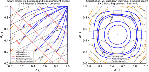
Figure 5. Euclidean (orange) vs. Shahshahani (blue) individual payoff gradients in a $2\times 2$ potential and harmonic game (left and right respectively). Dark dotted lines represent payoff contours, and red dotted lines (left figure only) represent contours of the potential function. The replicator dynamical system (C.16) is equivalent to individual Shahshahani gradient ascent; the figure shows how the functional form of the inverse Shahshahani metric given by Eq. C.15, decaying to zero as the boundary is approached, is the key feature that confines replicator dynamics (blue) to the interior of the strategy space, whereas Euclidean steepest individual payoff ascent (orange) leads to hitting the boundary in finite time. The payoffs used in these examples are $u_{1}=(2,0,3,1),u_{2}=(2,3,0,1)$ in Prisoner’s Dilemma, that is potential with potential function $\phi=(-1,0,0,1)$; and $u_{1}=(3,-3,-3,3),u_{2}=(-3,3,3,-3)$ in rescaled Matching Pennies, that is harmonic.

In a $2\times 2$ game the effective strategy space of each player is one dimensional, i.e., $\mu_{i}$ and $\nu_{i}$ belong to the singleton $\{1_{i}\}$ for $i\in\{1,2\}$. As discussed in Example B.1 the two reduced payoff fields, with one component each, are

$$\tilde{v}_{1}(\tilde{x}_{1},\tilde{x}_{2})=\tilde{x}_{2}\big{[}u_{1}(0,0)-u_{1}(0,1)-u_{1}(1,0)+u_{1}(1,1)\big{]}-u_{1}(0,0)+u_{1}(1,0)$$ (C.13)

$$\tilde{v}_{2}(\tilde{x}_{1},\tilde{x}_{2})=\tilde{x}_{1}\big{[}u_{2}(0,0)-u_{2}(0,1)-u_{2}(1,0)+u_{2}(1,1)\big{]}-u_{2}(0,0)+u_{2}(0,1)$$ (C.14)

By Eq. C.11 the effective inverse Shahshahani metric on each $1$-dimensional open corner of cube $\mathcal{C}^{\circ}=(0,1)\subset\mathbb{R}$ has only one component given by

$$\begin{split}\tilde{g}_{1}^{-1}(\tilde{x}_{1},\tilde{x}_{2})&=\tilde{x}_{1}(1-\tilde{x}_{1})\\ \tilde{g}_{2}^{-1}(\tilde{x}_{1},\tilde{x}_{2})&=\tilde{x}_{2}(1-\tilde{x}_{2})\end{split}$$ (C.15)

This functional form of the inverse Shahshahani metric is the key feature alluded at in Remark B.3 that confines the replicator dynamics to the interior of the strategy space $\mathcal{C}$, as opposed to steepest individual payoff ascent with respect to the Euclidean metric, that leads to hitting the boundary in finite time. Expanding $\tilde{g}^{-1}_{i}$ around $\tilde{x}_{i}=0.5$ we see that $\tilde{g}^{-1}_{i}(\tilde{x})\approx 0.25$, i.e., toward the middle of the open corner of cube $\mathcal{C}^{\circ}$ the Shahshahani metric is just a rescaled version of the Euclidean metric $\tilde{g}^{-1}_{i}=1$. On the other hand $\lim_{\tilde{x}_{i}\to 0_{+}}\tilde{g}^{-1}_{i}(\tilde{x})=\lim_{\tilde{x}_{i}\to 1_{-}}\tilde{g}^{-1}_{i}(\tilde{x})=0$, i.e., toward the boundary of $\mathcal{C}^{\circ}$ the inverse Shahshahani metric goes to zero, dampening the dynamics and bounding it to the interior of $\mathcal{C}$:

$$\begin{cases}\tilde{v}^{\sharp}_{1}(\tilde{x})=\dot{\tilde{x}}_{1}=\tilde{g}_{1}^{-1}\tilde{v}_{1}=\tilde{x}_{1}(1-\tilde{x}_{1})\tilde{v}_{1}(\tilde{x})=\tilde{x}_{1}\left[\tilde{v}_{1}(\tilde{x})-\tilde{x}_{1}\,\tilde{v}_{1}(\tilde{x})\right]\\ \tilde{v}^{\sharp}_{2}(\tilde{x})=\dot{\tilde{x}}_{2}=\tilde{g}_{2}^{-1}\tilde{v}_{2}=\tilde{x}_{2}(1-\tilde{x}_{2})\tilde{v}_{2}(\tilde{x})=\tilde{x}_{2}\left[\tilde{v}_{2}(\tilde{x})-\tilde{x}_{2}\,\tilde{v}_{2}(\tilde{x})\right]\end{cases}$$ (C.16)

which are Eq. 28 for a $2\times 2$ game (cf. Remark B.2 for the notation). The orbits of this dynamical system are plotted in Fig. 5 for Prisoner’s Dilemma (potential) and Matching Pennies (harmonic). $\diamond$

C.3. Differential characterizations of potential games

We conclude this appendix with two characterizations of exact potential games in the sense of Monderer & Shapley [66].

Definition 7.

The effective payoff field $\tilde{v}$ of a finite game $\Gamma(\mathcal{N},\mathcal{A},u)$ is called exact if it is the differential of a function, namely if there exist a function $\phi\colon\mathcal{A}\to\mathbb{R}$, called potential, such that $\tilde{v}_{i}(\tilde{x})=\tilde{d}_{i}\tilde{\phi}(\tilde{x})$ for all $\tilde{x}\in\mathcal{C}$ and all $i\in\mathcal{N}$.

Remark C.2.

We denote a function $\phi\colon\mathcal{A}\to\mathbb{R}$ and its multilinear extension $\phi\colon\mathcal{X}\to\mathbb{R}$, $\phi(x)=\sum_{\alpha}x_{\alpha}\phi(\alpha)$ by the same symbol, and it is understood that it is the multilinear extension undergoing differentiation. As in Remark B.1, the differential $d{f}$ of a differentiable function $f$ is the array of partial derivatives of the function. A tilde denotes as usual effective objects, and $\tilde{d}_{i}$ denotes the array of partial derivatives with respect to the $\tilde{x}_{i}$ coordinates. $\diamond$

Recall from the main text that a finite game $\Gamma$ is exact-potential in the sense of Monderer & Shapley [66] if it admits a potential function $\phi\colon\mathcal{X}\to\mathbb{R}$ such that

$$u_{i}(\beta_{i};\alpha_{-i})-u_{i}(\alpha_{i};\alpha_{-i})=\phi(\beta_{i};\alpha_{-i})-\phi(\alpha_{i};\alpha_{-i})$$ (PG)

for all $\alpha,\beta\in\mathcal{A}$ and all $i\in\mathcal{N}$. The notion of exactness for the effective payoff field allows for an equivalent characterization:

Lemma C.2.

A finite game $\Gamma(\mathcal{N},\mathcal{A},u)$ is exact-potential in the sense of Monderer & Shapley [66] if and only if its effective payoff field $\tilde{v}$ is exact.

Proof.

Assume that $\tilde{v}$ is exact with potential $\phi$. Then by chain rule $\tilde{v}_{i\mu_{i}}(\tilde{x})=\tilde{\partial}_{i\mu_{i}}\tilde{\phi}(\tilde{x})=(\partial_{i\mu_{i}}-\partial_{i0_{i}})\phi(x)$, for all $i\in\mathcal{N}$, $\mu_{i}\in\{1,\dots,m_{i}\}$, and $\tilde{x}\in\mathcal{C}$. Since $\tilde{v}_{i\mu_{i}}(\tilde{x})=v_{i\mu_{i}}(x)-v_{i0_{i}}(x)$ we conclude that $u_{i}(\alpha_{i},x_{-i})-u_{i}(0_{i},x_{-i})=\phi(\alpha_{i},x_{-i})-\phi(0_{i},x_{-i})$ for all $i\in\mathcal{N}$, $\alpha_{i}\in\{0,\dots,m_{i}\}$, and $x\in\mathcal{X}$, implying in turn that the game is potential by Lemma B.4. Conversely, assume that $\Gamma(\mathcal{N},\mathcal{A},u)$ is potential; then the sequence of arguments is reversed without any change, showing that $\tilde{v}$ is exact. ∎

In the context of population games this result can be found in Sandholm [74, Chapter 3.2.2]. The interpretation of this lemma is the following: Recall by Eq. B.5 that the the effective payoff field $\tilde{v}$ of a game is the array of individual differentials of the effective payoff functions, i.e., $\tilde{v}=\left(\tilde{d}_{i}\tilde{u}_{i}\right)_{i\in\mathcal{N}}$. As such, in general $\tilde{v}$ is not the differential of a function; Lemma C.2 says that a game is potential precisely when this is the case, namely when $\tilde{v}=\left(\tilde{d}_{i}\tilde{\phi}\right)_{i\in\mathcal{N}}=\tilde{d}\tilde{\phi}$.

The differential characterization of potential games given above, relying on the notion of exact effective payoff field, is intrinsic of a game and independent of any choice of metric. Yet, if a Riemannian metric on $\mathcal{X}^{\circ}$ is available, the metric’s non-degeneracy allows for another characterization of potential games, in a sense dual to the one given above.

Given a Riemannian metric $g$ on $\mathcal{X}^{\circ}$, and leveraging Lemma A.1 relating the gradient and the differential of a function via the matrix of the metric, we say that a vector field $F$ on $\mathcal{X}^{\circ}$ is the gradient of a function $\phi$ if $F=g^{-1}\cdot d\phi$, where $\cdot$ denotes matrix multiplication. With this in mind we can give the following

Lemma C.3.

Given a Riemannian metric $g$ on $\mathcal{X}^{\circ}$, a finite game $\Gamma(\mathcal{N},\mathcal{A},u)$ is an exact potential game if and only if its field of effective individual payoff gradients, denoted by $\tilde{v}^{\sharp}$, is the gradient of a function, namely if there exists a function $\phi\colon\mathcal{A}\to\mathbb{R}$ such that $\tilde{v}^{\sharp}=\tilde{g}^{-1}\cdot\tilde{d}\tilde{\phi}$.

Proof.

The field of effective individual payoff gradients of a game is

$$\tilde{v}^{\sharp}=\left(\tilde{g}_{i}^{-1}\cdot\tilde{d}_{i}\tilde{u}_{i}\right)_{i\in\mathcal{N}}=\left(\tilde{g}_{i}^{-1}\cdot\tilde{v}_{i}\right)_{i\in\mathcal{N}}\,.$$ (C.17)

This field is a gradient if there exists a function $\phi\colon\mathcal{A}\to\mathbb{R}$ such that

$$\tilde{v}^{\sharp}=\tilde{g}^{-1}\cdot\tilde{d}\tilde{\phi}=\left(\tilde{g}_{i}^{-1}\cdot\tilde{d}_{i}\tilde{\phi}\right)_{i\in\mathcal{N}}\,,$$ (C.18)

where $\tilde{\phi}\colon\mathcal{C}\to\mathbb{R}$ is the effective representation of the multilinear extension of $\phi\colon\mathcal{A}\to\mathbb{R}$. By non degeneracy of the Riemannian metric $g$, the effective field of individual gradients is a gradient if and only if $\tilde{v}_{i}=\tilde{d}_{i}\tilde{\phi}$ for all $i\in\mathcal{N}$, i.e., if the effective payoff field is exact, which is equivalent to $\Gamma(\mathcal{N},\mathcal{A},u)$ being an exact potential game by Lemma C.2. ∎

An example of this result is given by Kimura’s maximum principle [47, 75], which states that, in potential games, replicator dynamics (that is, the dynamics given by the field of individual payoff Shahshahani gradients) is a Shahshahani gradient system. Lemma C.3 provides a broad generalization of this principle: in a potential game, given any metric $g$, the dynamics given by the field of individual payoff $g$-gradients is a $g$-gradient dynamics in its own right.

Full potential games

By Lemma C.2, a finite game in normal form is potential if and only if its effective payoff field is exact. In the context of population games, Sandholm [74, Chapter 3.1] calls a game such that the full payoff field is exact, i.e., $v=d\phi$, a full potential game. One can show that if the full payoff field of the game is exact then the effective payoff field is exact too, but the converse needs not be true. In other words, $v=d\phi$ is a sufficient but not necessary condition for a game to be potential. We illustrate this fact with a simple example; for further details on the relation between potential games and full potential games we refer the reader to Sandholm [74, Chapter 3.2.3].

Example C.2.

Consider the $2\times 2$ potential game with payoffs $u$ and potential function $\phi$ given by

$$u=\begin{pmatrix}(2,2)&(0,3)\\ (3,0)&(1,1)\\ \end{pmatrix},\quad\phi=\begin{pmatrix}-1&0\\ 0&1\\ \end{pmatrix}\,.$$ (C.19)

The corresponding replicator dynamics are plotted in Fig. 5, left. Replacing for notational simplicity $(x_{1,0},x_{1,1})\to(x_{0},x_{1})$ and $(x_{2,0},x_{2,1})\to(y_{0},y_{1})$ we have from Example B.1 that the full payoff field is

$$v(x_{0},x_{1},y_{0},y_{1})=\left(2y_{0},\,3y_{0}+y_{1},\,2x_{0},\,3x_{0}+x_{1}\right)\,.$$ (C.20)

A simple check shows that $\partial_{y_{0}}v_{x_{1}}=3\neq 0=\partial_{x_{1}}v_{y_{0}}$ which, by a routine application of Poincaré’s lemma [41], implies that $v$ is not the differential of a function. On the other hand, the reduced payoff field is

$$\tilde{v}(\tilde{x}_{1},\tilde{y}_{1})=(1,1)\,,$$ (C.21)

which is exact, since it is the differential of any function $\tilde{\phi}(\tilde{x}_{1},\tilde{y}_{1})=\tilde{x}_{1}+\tilde{y}_{1}+\text{const}$. Note that the multilinear extension of the potential function of the game is $\phi(x_{0},x_{1},y_{0},y_{1})=-x_{0}y_{0}+x_{1}y_{1}$, and its reduced form is $\phi(\tilde{x}_{1},\tilde{y}_{1})=-(1-\tilde{x}_{1})(1-\tilde{y}_{1})+\tilde{x}_{1}\tilde{y}_{1}=\tilde{x}_{1}+\tilde{y}_{1}-1$, showing that, albeit the full payoff field is not exact, the reduced payoff field is the differential of the reduced multilinear extension of the potential function of the game.

Appendix D Proofs on incompressible games

The results presented here heavily rely on the mathematical tools of Appendix A, which we therefore recommend reading first.

D.1. Shahshahani divergence

In this section we prove the results given in Section 5. They all revolve around the expression of the Shahshahani divergence of the effective replicator field that – as discussed in more detail in Section A.3 – is given by Eq. 27 from the main text:

$$\operatorname{div}_{i}v^{\sharp}_{i}(\tilde{x})=\frac{1}{\sqrt{\det\tilde{g}_{i}(\tilde{x}_{i})}}\sum_{\mu_{i}=1}^{m_{i}}\frac{\partial}{\partial\tilde{x}_{i\mu_{i}}}\left(\sqrt{\det\tilde{g}_{i}(\tilde{x}_{i})}\,v^{\sharp}_{i\mu_{i}}(\tilde{x})\right)\quad\text{for all }i\in\mathcal{N}\,.$$ (27)

By Lemma A.3, the divergence operator on a product manifold - which in our case is the product $\mathcal{C}^{\circ}=\prod_{i}\mathcal{C}^{\circ}_{i}$ of open corner of cubes, where the effective game described in Appendix B lives - is given by the sum of the divergence operators on the factor manifolds, which justifies Definition 1 of incompressible games given in Section 4: See 1 We devote the rest of this section to the proof of the following result:

Proposition D.1.

The Shahshahani divergence of the effective replicator field of a finite game $\Gamma(\mathcal{N},\mathcal{A},u)$ is

$$\operatorname{div}v^{\sharp}(\tilde{x})=+\frac{1}{2}\sum_{i\in\mathcal{N}}\sum_{\alpha_{i}\in\mathcal{A}_{i}}\left(v_{i\alpha_{i}}(x)-u_{i}(x)\right)\,.$$ (D.1)

Proof.

To prove this result we will first compute $\operatorname{div}_{i}{v^{\sharp}_{i}}(\tilde{x})$ for some $i\in\mathcal{N}$, dropping the index $i$ for notational simplicity. Recall by Eq. A.6 that the expression for the divergence can be rewritten by product rule as the sum of two terms, one metric-dependent and one metric-independent:

$$\operatorname{div}_{i}{v^{\sharp}_{i}}(\tilde{x})\overbrace{\equiv}^{\text{Drop }i\text{ index}}\operatorname{div}{v^{\sharp}}(\tilde{x})=\sum_{\mu=1}^{m}\left(\frac{\partial_{\tilde{x}_{\mu}}\sqrt{\det{\tilde{g}}}}{\sqrt{\det{\tilde{g}}}}\right)v^{\sharp}_{\mu}(\tilde{x})+\sum_{\mu=1}^{m}\partial_{\tilde{x}_{\mu}}v^{\sharp}_{\mu}(\tilde{x})\,,$$ (D.2)

where $\partial_{\tilde{x}_{\mu}}$ is a shorthand for $\frac{\partial}{\partial\tilde{x}_{\mu}}$, and $\det{\tilde{g}}$ is given by Eq. B.26:

$$\det{\tilde{g}}(\tilde{x})=\frac{1}{\left(1-\sum_{\mu=1}^{m}\tilde{x}_{\mu}\right)\prod_{\nu=1}^{m}\tilde{x}_{\nu}}=\frac{1}{x_{0}\prod_{\nu=1}^{m}\tilde{x}_{\nu}}\,.$$ (B.26)

Metric-independent term of the divergence

Denote by $\bar{v}(x)\coloneqq\sum_{\alpha}x_{\alpha}v_{\alpha}(x)$, and by $\bar{\tilde{v}}(\tilde{x})\coloneqq\sum_{\mu}\tilde{x}_{\mu}\tilde{v}_{\mu}(\tilde{x})$, so that the full and effective replicator dynamics (with player index suppressed) read

$$\dot{x}_{\alpha}=v^{\sharp}_{\alpha}(x)=x_{\alpha}\left[v_{\alpha}(x)-\bar{v}(x)\right]\quad\text{ for all }\alpha=0,\dots,m\,,$$ (D.3a)

$$\dot{\tilde{x}}_{\mu}=v^{\sharp}_{\mu}(\tilde{x})=\tilde{x}_{\mu}\left[\tilde{v}_{\mu}(\tilde{x})-\bar{\tilde{v}}(\tilde{x})\right]\quad\text{ for all }\mu=1,\dots,m\,.$$ (D.3b)

Remark D.1.

Reinserting for the scope of this remark the player index, a simple check shows that $\bar{\tilde{v}}_{i}(\tilde{x})=\bar{v}_{i}(x)-v_{i0_{i}}(x)$; note that $\bar{v}_{i}(x)$ is precisely the full payoff function $u_{i}(x)$, while $\bar{\tilde{v}}_{i}(\tilde{x})$ is not the effective payoff function $\tilde{u}_{i}(\tilde{x})$, the difference between the two being precisely $v_{i0_{i}}(x)$. $\diamond$

As usual, the indices $\mu$ and $\nu$ appearing in the following expressions are understood to run over $1,\dots,m$; and the indices $\alpha$ and $\beta$ are understood to run over $0,\dots,m$. With these notational caveats in place, the metric-independent term of the divergence reads

$$\begin{split}\sum_{\mu}\partial_{\tilde{x}_{\mu}}v^{\sharp}_{\mu}(\tilde{x})&=\sum_{\mu}\partial_{\tilde{x}_{\mu}}\Big{(}\tilde{x}_{\mu}(\tilde{v}_{\mu}(\tilde{x})-\bar{\tilde{v}}(\tilde{x}))\Big{)}\\ &=\sum_{\mu}(\tilde{v}_{\mu}-\bar{\tilde{v}})+\sum_{\mu}\tilde{x}_{\mu}\partial_{\tilde{x}_{\mu}}\tilde{v}_{\mu}-\bar{\tilde{v}}-\sum_{\mu\nu}\tilde{x}_{\mu}\tilde{x}_{\nu}\partial_{\tilde{x}_{\mu}}\tilde{v}_{\nu}\,.\\ \end{split}$$ (D.4)

By Lemma B.3 the second and fourth terms vanish: re-inserting the player index $i\in\mathcal{N}$, $\frac{\partial\tilde{v}_{i\nu_{i}}}{\partial\tilde{x}_{i\mu_{i}}}(\tilde{x})\equiv 0$ since the components of the reduced payoff field of player $i\in\mathcal{N}$ do not depend on the mixed coordinates of player $i$. This leads to

$$\sum_{\mu}\partial_{\tilde{x}_{\mu}}v^{\sharp}_{\mu}(\tilde{x})=\sum_{\mu}\left(v_{\mu}-v_{0}-\bar{v}+v_{0}\right)-\bar{v}+v_{0}=\sum_{\alpha}(v_{\alpha}-\bar{v})\,,$$ (D.5)

and in conclusion the metric-independent term of the divergence $\operatorname{div}{v^{\sharp}}(\tilde{x})$ is

$$\sum_{\mu}\partial_{\tilde{x}_{\mu}}v^{\sharp}_{\mu}(\tilde{x})=\sum_{\alpha}\left(v_{\alpha}(x)-\bar{v}(x)\right)\,,$$ (D.6)

where it is understood that effective objects (i.e., containing the effective payoff field $\tilde{v}$) are evaluated at $\tilde{x}$, and full objects (i.e., containing the full payoff field $v$) are evaluated at $x$, with $x$ and $\tilde{x}$ related as usual by the map $\pi_{0}$ of Eq. B.2.

In settings with non-multilinear utility functions, such as games with continuous action sets and differentiable payoff functions [55, 62, 73], the terms of Eq. D.4 containing derivatives of the payoff field do not necessarily vanish; as a reference for possible applications to these settings we provide below the version of Eq. D.6 including such terms. To this end denote by $B=J{\tilde{v}}$ the Jacobian matrix of the effective payoff field, i.e., $B_{\nu\mu}=\partial_{\tilde{x}_{\mu}}\tilde{v}_{\nu}$, and recall that $\tilde{v}_{\mu}=v_{\mu}-v_{0}$ to rewrite Eq. D.4 as

$$\sum_{\mu}\partial_{\tilde{x}_{\mu}}v^{\sharp}_{\mu}(\tilde{x})=\sum_{\alpha}(v_{\alpha}-\bar{v})+\left(\sum_{\mu}\tilde{x}_{\mu}B_{\mu\mu}-\sum_{\mu\nu}\tilde{x}_{\mu}\tilde{x}_{\nu}B_{\mu\nu}\right)\,.$$ (D.7)

The idea now is that of re-arranging the terms that contain effective coordinates $\tilde{x}$ and combine them into objects expressed in terms of full coordinates $x$. After a straightforward but tedious computation leveraging Lemma B.2 the second term on the right hand side can be expressed in terms of full objects as

$$\sum_{\mu}\tilde{x}_{\mu}B_{\mu\mu}-\sum_{\mu\nu}\tilde{x}_{\mu}\tilde{x}_{\nu}B_{\mu\nu}=\sum_{\alpha}x_{\alpha}\partial_{\alpha}v_{\alpha}-\sum_{\alpha\beta}x_{\alpha}x_{\beta}\partial_{\alpha}v_{\beta}\,.$$ (D.8)

Metric-dependent term of the divergence

A direct computation shows that

$$\frac{\partial_{\tilde{x}_{\mu}}\sqrt{\det{\tilde{g}}}}{\sqrt{\det{\tilde{g}}}}=-\frac{1}{2}\frac{\tilde{x}_{0}-\tilde{x}_{\mu}}{\tilde{x}_{0}\tilde{x}_{\mu}}\,.$$ (D.9)

Again, one needs to manipulate the terms containing effective coordinates to express them in terms of full coordinates. After an elementary but lengthy calculation, we obtain that the metric-dependent term of the divergence $\operatorname{div}{v^{\sharp}}(\tilde{x})$ is

$$\sum_{\mu}v^{\sharp}_{\mu}(\tilde{x})\,\frac{\partial_{\tilde{x}_{\mu}}\sqrt{\det{\tilde{g}}}}{\sqrt{\det{\tilde{g}}}}(\tilde{x})=-\frac{1}{2}\sum_{\alpha}\left(v_{\alpha}(x)-\bar{v}(x)\right)\,.$$ (D.10)

Conclusion

Summing Eqs. D.10 and D.6 and re-inserting the player index we finally get

$$\operatorname{div}_{i}v^{\sharp}_{i}(\tilde{x})=+\frac{1}{2}\sum_{\alpha_{i}\in\mathcal{A}_{i}}\left(v_{i\alpha_{i}}(x)-u_{i}(x)\right)\,,$$ (D.11)

and the proof is completed by summing over the player index $i\in\mathcal{N}$. ∎ To conclude this section we provide an equivalent expression for the Shahshahani divergence of the effective replicator field. For all $i\in\mathcal{N}$ define the barycenter $\mathbf{b}_{i}\in\mathcal{X}_{i}$ as the point with coordinates

$$\mathbf{b}_{i\alpha_{i}}\coloneqq\frac{1}{A_{i}}\quad\text{for all }\alpha_{i}\in\mathcal{A}_{i}$$ (D.12)

on the mixed strategy space $\mathcal{X}_{i}$ of player $i\in\mathcal{N}$, where $A_{i}=\lvert\mathcal{A}_{i}\rvert$ is the number of pure strategies of player $i$. Similarly, define $\mathbf{1}_{i}\coloneqq(1,\dots,1)\in\mathbb{R}^{A_{i}}$. Then

Lemma D.1 (Equivalent expression of the Shahshahani divergence).

The Shahshahani divergence of the effective replicator field of a finite game $\Gamma(\mathcal{N},\mathcal{A},u)$ fulfills

$$-\operatorname{div}v^{\sharp}(\tilde{x})=\frac{1}{2}\sum_{i\in\mathcal{N}}\sum_{\alpha_{i}\in\mathcal{A}_{i}}\left(u_{i}-v_{i\alpha_{i}}\right)(x)=\frac{1}{2}\sum_{i}A_{i}\,v_{i}(x)\cdot\left(x_{i}-\mathbf{b}_{i}\right)\,.$$ (D.13)

Proof.

From Proposition D.1 and the application of definitions it follows that

$$\begin{split}-\operatorname{div}v^{\sharp}(\tilde{x})&=\frac{1}{2}\sum_{i\in\mathcal{N}}\sum_{\alpha_{i}\in\mathcal{A}_{i}}\left(u_{i}-v_{i\alpha_{i}}\right)(x)=\frac{1}{2}\sum_{i}\left(A_{i}u_{i}-v_{i}\cdot\mathbf{1}_{i}\right)(x)\\ &=\frac{1}{2}\sum_{i}A_{i}\left(u_{i}-v_{i}\cdot\mathbf{b}_{i}\right)(x)=\frac{1}{2}\sum_{i}A_{i}\,v_{i}(x)\cdot\left(x_{i}-\mathbf{b}_{i}\right)\,.\qed\end{split}$$ (D.14)

D.2. Incompressible games are precisely harmonic games

The expression of the Shahshahani divergence of the field of individual Shahshahani payoff gradients of a game $\operatorname{div}v^{\sharp}(\tilde{x})$ allows to establish an important connection between incompressible games, i.e., those game for which $\operatorname{div}v^{\sharp}$ vanishes identically, and the harmonic games introduced by Candogan et al. [14]. Recall by Eq. HG that a game is harmonic if

$$\sum\nolimits_{i\in\mathcal{N}}\sum\nolimits_{\beta_{i}\in\mathcal{A}_{i}}[u_{i}(\beta_{i};\alpha_{-i})-u_{i}(\alpha_{i};\alpha_{-i})]=0$$ (HG)

for all $\alpha\in\mathcal{A}$. With this at hand we can prove Theorem 2: See 2

Proof.

Begin by noting that the Eq. HG characterizing harmonic games can be recast as $F(\alpha)=0$ for all $\alpha\in\mathcal{A}$, with $F\colon\mathcal{A}\to\mathbb{R}$ defined by

$$F(\alpha) \coloneqq\sum_{i\in\mathcal{N}}\sum_{\beta_{i}\in\mathcal{A}_{i}}\Big{(}u_{i}(\beta_{i},\alpha_{-i})-u_{i}(\alpha_{i},\alpha_{-i})\Big{)}$$

$$=\sum_{i}\left[\left(\sum_{\beta_{i}}u_{i}(\beta_{i},\alpha_{-i})\right)-A_{i}u_{i}(\alpha)\right]\,.$$ (D.15)

We claim that the Shahshahani divergence of the effective replicator field of a finite game is (up to a factor of $1/2$) the multilinear extension of the function $F$ defined above:

$$\operatorname{div}v^{\sharp}(\tilde{x})=\frac{1}{2}\bar{F}(x)\coloneqq\frac{1}{2}\sum_{\alpha\in\mathcal{A}}x_{\alpha}F(\alpha)\,,$$ (D.16)

for all $\tilde{x}\in\mathcal{C}$. If we show this the proof is concluded, since invoking Lemma B.4 we have

harmonic $$\iff F\equiv 0\,,$$

incompressible $$\iff\bar{F}\equiv 0\,,$$

$$F\equiv 0 \iff\bar{F}\equiv 0\,.$$ (D.17)

Eq. D.16 is verified by a standard multilinear calculation:

$$\bar{F}(x) =\sum_{\alpha\in\mathcal{A}}x_{\alpha}F(\alpha)=\sum_{i}\left[\left(\sum_{\beta_{i}}u_{i}(\beta_{i},x_{-i})\right)-A_{i}u_{i}(x)\right]=\sum_{i}\left(v_{i}\cdot\mathbf{1}_{i}-A_{i}u_{i}\right)(x)$$ (D.18)

for all $x\in\mathcal{X}$; so from Lemma D.1 we have that $\operatorname{div}v^{\sharp}=1/2\bar{F}$, concluding the proof. ∎

Having established the equivalence between harmonic and incompressible games, the following decomposition result comes as an immediate corollary of the strategic decomposition (5): See 1

Proof.

As shown by Candogan et al. [14] every finite game can be decomposed as the sum of a potential and a harmonic game, which gives the decomposition $\Gamma=\Gamma_{\!\textup{pot}}+\Gamma_{\!\textup{inc}}$ in light of the fact that a game is incompressible if and only if it is harmonic.

As for the second point, the field of individual gradients of the incompressible game $\Gamma_{\!\textup{inc}}$ is incompressible by definition; and Lemma C.3 asserts that a game is an exact potential game in the sense of Monderer & Shapley [66] if and only if its effective field of individual gradients is the Riemannian gradient of a function $\phi$, i.e., the field $v^{\sharp}$ of the potential game $\Gamma_{\!\textup{pot}}$ can be expressed as $\operatorname{grad}{\phi}$. ∎

D.3. Dynamics on incompressible games and Poincaré’s recurrence

Finally we turn our attention at the dynamical properties of replicator dynamics on incompressible games; our first result is a consequence of the Riemannian version of Liouville’s theorem presented in Section A.4. See 2

Proof.

By definition, a game is incompressible if and only if the Shahshahani divergence of the field $v^{\sharp}(\tilde{x})$ vanishes identically. Since (RD) is the dynamical system on $\mathcal{C}^{\circ}$ given by $\dot{\tilde{x}}=v^{\sharp}(\tilde{x})$, as a consequence of Liouville’s theorem (cf. Eq. A.13) we have that $\operatorname{vol}(\mathcal{U}_{t})=\operatorname{vol}(\mathcal{U})$ for all open sets $\mathcal{U}\subseteq\mathcal{C}^{\circ}$ and all $t\in\mathbb{R}$, meaning that (RD) is volume-preserving with respect to the Shahshahani volume form. ∎

Our next result shows that replicator dynamics on incompressible games admit a constant of motion. See 3

Proof.

For each $i\in\mathcal{N}$ consider the Kullback–Leibler divergence with respect to the barycenter $\operatorname{KL}_{\mathbf{b}_{i}}\colon\mathcal{X}^{\circ}_{i}\to\mathbb{R}$,

$$\operatorname{KL}_{\mathbf{b}_{i}}(x_{i})=\sum_{\alpha_{i}\in\mathcal{A}_{i}}\mathbf{b}_{i\alpha_{i}}\log{\frac{\mathbf{b}_{i\alpha_{i}}}{x_{i\alpha_{i}}}}\,.$$ (D.19)

and scale it by the number $A_{i}$ of pure strategies of player $i$:

$$E_{i}(x_{i})\coloneqq A_{i}\operatorname{KL}_{\mathbf{b}_{i}}(x_{i})=-\left(A_{i}\log{A_{i}}+\sum_{\alpha_{i}\in\mathcal{A}_{i}}\log{x_{i\alpha_{i}}}\right)\,.$$ (D.20)

The derivative of $E_{i}$ along a solution trajectory of (RD) is $\frac{d}{dt}E_{i}(x_{i}(t))=-\sum_{\alpha_{i}\in\mathcal{A}_{i}}\frac{\dot{x}_{i\alpha_{i}}}{x_{i\alpha_{i}}}=-\sum_{\alpha_{i}\in\mathcal{A}_{i}}[v_{i\alpha_{i}}(x)-u_{i}(x)]$, so by Proposition D.1,

$$\operatorname{div}v^{\sharp}(\tilde{x}(t))=-\frac{1}{2}\frac{d}{d{t}}\sum_{i\in\mathcal{N}}E_{i}(x_{i}(t))\quad\text{along RD}\,.$$ (D.21)

It follows that the $A_{i}$-weighted sum $E\colon\mathcal{X}^{\circ}\to\mathbb{R}$ of Kullback–Leibler divergences with respect to the barycenter,

$$E(x)\coloneqq\sum_{i\in\mathcal{N}}E_{i}(x_{i})=\sum_{i\in\mathcal{N}}A_{i}\operatorname{KL}_{\mathbf{b}_{i}}(x_{i})=-\left(\sum_{i\in\mathcal{N}}\sum_{\alpha_{i}\in\mathcal{A}_{i}}\log{x_{i\alpha_{i}}}+\text{const}\right)\,,$$ (D.22)

is a constant of motion for the (EW) / (RD) dynamics on incompressible games, with $\text{const}=\sum_{i}A_{i}\log{A_{i}}$. ∎

The function $E\colon\mathcal{X}^{\circ}\to\mathbb{R}$ is a nonnegative weighted sum of convex functions, hence it is convex. Its sublevel sets are then compact convex sets, and as such homeomorphic to closed balls, making in turn their boundaries – the level sets of $E$ – homeomorphic to $\left[(\sum_{i}A_{i})-N-1\right]$-dimensional spheres. Since RD solution trajectories are constrained to the level sets of the integral of motion $E$, this shows that $\mathcal{X}^{\circ}$ admits a foliation under replicator dynamics on harmonic games with leaves given by concentric topological spheres, as mentioned in Section 5 in the main body of the article.

Remark D.2 (Harmonic vs. zero-sum games).

In two-player ZSGs with an interior Nash equilibrium $x^{\ast}$ the sum of Kullback-Leibler divergences with respect to said equilibrium, $\sum_{i}\operatorname{KL}_{x^{\ast}_{i}}(x_{i})$, is a constant of motion for replicator dynamics [63]. Harmonic games and ZSGs have non-trivial intersection; in particular, normalized harmonic games where all players have the same number of strategies are zero-sum [14]. In this case the $A_{i}$-s factor out from Eq. D.22, and the two constants of motions coincide, up to affine transformations.

Despite having non-trivial intersection, harmonic and ZSGs exhibit some very different properties. A ZSG can also be a potential game, while the only harmonic game which admits a potential is the zero game (up to strategic equivalence)[14]; Harmonic games always admit a fully mixed equilibrium [14], while ZSGs do not (that is, not always); ZSGs may admit strict Nash equilibria, while harmonic games never do; replicator dynamics are recurrent in ZSGs with a fully mixed equilibrium [63] but convergent in ZSGs with a strict equilibrium [60], while they are always recurrent in harmonic games (Theorem 4). As minimal example setting apart harmonic and zero-sum games consider the $2\times 3$ game with payoffs

$$u_{1}=\begin{pmatrix}a&b&-a-b\\ -a&-b&a+b\end{pmatrix}\quad\text{and}\quad u_{2}=-\frac{2}{3}u_{1}\,.$$ (D.23)

This game is is harmonic for every choice of $a,b\in\mathbb{R}$, and never zero-sum (except for the trivial case). $\diamond$

Poincaré recurrence in mixed strategy space

We turn now to our last result, namely to the fact that replicator dynamics on harmonic games are recurrent in the sense of Poincaré [70].

Several works in the literature [63, 69] discuss Poincaré recurrence in the context of zero-sum games with an interior Nash equilibrium, and positive affine transformations or polymatrix/network versions of the above. The idea is to transform via a suitable diffeomorphism the replicator system in the interior of the strategy space to a system which is divergence-free under the Euclidean metric; and to show that, under this transformations, all the orbits of RD in the particular class of games at hand are bounded, e.g., by exhibiting a constant of motion with bounded level sets.

We tackle the problem from a different angle: our proof relies on the fact that in harmonic games the replicator system itself – without undergoing any transformation – is volume-preserving under the Shahshahani metric, and that the Shahshahani volume of the space of mixed strategies is finite; the conclusion then follows from the Riemannian versions of Poincaré’s theorem presented in Section A.4.

See 4

Proof.

By Remark A.4, Poincaré’s theorem applies to a Riemannian manifold $(\mathcal{M},g)$ given that (itn) there is a volume preserving map $\phi\colon\mathcal{M}\to\mathcal{M}$, and (itn) the manifold has finite $g$-volume . By Proposition 2, the flow of the replicator vector field $\tilde{v}^{\sharp}$ on incompressible (i.e., harmonic) games is volume-preserving with respect to the effective Shahshahani metric on the open corner of cube. Hence, if we show that the Shahshahani volume of the open corner of cube is finite, namely that $\operatorname{vol}_{\text{Sha}}{\mathcal{C}^{\circ}}<\infty$, by Poincaré’s theorem we can conclude that the solution trajectories of replicator dynamics on incompressible games return arbitrarily close to almost every starting point $\tilde{x}\in\mathcal{C}^{\circ}$.

To show that the volume of the $m_{i}$-dimensional open corner of cube $\mathcal{C}^{\circ}_{m_{i}}$ with respect to the effective Shahshahani metric fulfills $\operatorname{vol}_{\text{Sha}}{\mathcal{C}^{\circ}_{m_{i}}}<\infty$ for all $i\in\mathcal{N}$ and all natural $m_{i}$ we resort to a transformation first introduced by Akin [2, p. 39] and discussed e.g., by Sandholm [74, p. 228] and Laraki & Mertikopoulos [51, Example 3.1]. Suppressing for a moment the player index, Akin [2] shows that the map $A\colon\mathbb{R}^{m+1}_{>0}\to\mathbb{R}^{m+1}_{>0}$, $A_{\alpha}(x)=2\sqrt{x_{\alpha}}$ for $\alpha\in\{0,\dots,m\}$, is an isometry between the $m$-dimensional open simplex $\mathcal{X}^{\circ}$ endowed with the Shahshahani metric and the portion of the radius-$2$ $m$-hypersphere in the positive hyperoctant of $\mathbb{R}^{m+1}$ endowed with the Euclidean metric. Isometries between Riemannian manifolds preserve volumes, so (reinstating the player index $i\in\mathcal{N}$) the Shahshahani volume of the $m_{i}$-dimensional open simplex is the Euclidean $m_{i}$-volume of the portion of the $m_{i}$-hypersphere of radius 2 in the positive orthant of $\mathbb{R}^{m_{i}+1}$, that is

$$\operatorname{vol}_{\text{Sha}}\mathcal{X}^{\circ}_{i}=\frac{\pi^{\frac{m_{i}+1}{2}}}{\Gamma(\frac{m_{i}+1}{2})}<\infty\text{ for all }m_{i}\in\mathbb{N}\text{ and }i\in\mathcal{N}\,,$$ (D.24)

where $\Gamma$ is the gamma function. By construction, the map $\iota_{0}\colon\mathcal{C}^{\circ}_{i}\to\mathcal{X}^{\circ}_{i}$ is an isometry between the open corner of cube with the reduced Shahshahani metric and the open simplex with the full Shahshahani metric, so Eq. D.24 gives also the sought-after volume of the open corner of cube, finite as required. Finally, since the volume of a product manifold is the product of the factor manifolds, we have that $\operatorname{vol}_{\text{Sha}}(\mathcal{C}^{\circ})=\prod_{i}\operatorname{vol}_{\text{Sha}}(\mathcal{C}^{\circ}_{i})<\infty$. ∎

Remark D.3.

An alternative formula to compute the volume of the open simplex under the Shahshahani metric is the following. Suppress the player index $i\in\mathcal{N}$ for notational simplicity, and let as usual $\mu,\nu\in\{1,\dots,m\}$. The determinant of the Shahshahani metric $\tilde{g}$ in its effective representation is given by Eq. B.26, so by Eq. A.11 the volume of the $m$-dimensional open corner of cube $\mathcal{C}^{\circ}_{m}$ with respect to the effective Shahshahani metric is

$$\begin{split}\operatorname{vol}_{\text{Sha}}{\mathcal{C}^{\circ}_{m}}&=\int_{\mathcal{C}^{\circ}}\sqrt{\det{\tilde{g}}}\,d{\tilde{x}}^{1}\dots d{\tilde{x}}^{m}\\ &=\int_{\tilde{x}_{1}>0,\,\dots,\,\tilde{x}_{m}>0,\,\sum_{\mu}\tilde{x}_{1}<1}\sqrt{\det{\tilde{g}}}\,d{\tilde{x}}^{1}\dots d{\tilde{x}}^{m}\\ &=\int_{\tilde{x}_{1}:0}^{1}\int_{\tilde{x}_{2}:0}^{1-\tilde{x}_{1}}\cdots\int_{\tilde{x}_{m}:0}^{1-\tilde{x}_{1}-\cdots-\tilde{x}_{m-1}}\frac{1}{\sqrt{\left(1-\sum_{\mu}\tilde{x}_{\mu}\right)\prod_{\nu}\tilde{x}_{\nu}}}d{\tilde{x}}^{m}\cdots d{\tilde{x}}^{1}\\ &=\int_{\tilde{x}_{1}=0}^{\xi_{1}}\frac{d{\tilde{x}}^{1}}{\sqrt{\tilde{x}_{1}}}\int_{\tilde{x}_{2}=0}^{\xi_{2}}\frac{d{\tilde{x}}^{2}}{\sqrt{\tilde{x}_{2}}}\cdots\int_{\tilde{x}_{m-1}=0}^{\xi_{m-1}}\frac{d{\tilde{x}}^{m-1}}{\sqrt{\tilde{x}_{m-1}}}\int_{\tilde{x}_{m}=0}^{\xi_{m}}\frac{d{\tilde{x}}^{m}}{\sqrt{\tilde{x}_{m}(\xi_{m}-\tilde{x}_{m})}}\,,\end{split}$$ (D.25)

with $\xi_{m}=1-\tilde{x}_{1}-\cdots-\tilde{x}_{m-1}$. One can check for a few values of $m$ that the integrals are in agreement with Eq. D.24, for example $\operatorname{vol}_{\text{Sha}}\mathcal{C}^{\circ}_{m=1}=\pi,\operatorname{vol}_{\text{Sha}}\mathcal{C}^{\circ}_{m=2}=2\pi,\operatorname{vol}_{\text{Sha}}\mathcal{C}^{\circ}_{m=3}=\pi^{2}$. $\diamond$

The proof of the fact replicator dynamics exhibit Poincaré recurrence in harmonic games relies on the facts that (itn) the flow of RD is Shahshahani-incompressible in the space of mixed strategies precisely in such games, and (itn) the Shahshahani volume of the open simplex is finite. Both of these phenomena are quite peculiar, as we discuss in the next section.

D.4. On the special nature of the Shahshahani geometry

We conclude this appendix with a discussion of the fact that the Shahshahani metric is intrinsically related to the replicator dynamics (cf. Proposition 1), but not at all to the simplicial complex of the game’s response graph endowed with the Euclidean metric. In particular, incompressible games are defined completely independently of the harmonic games of Candogan et al. [14], and it is only through the lengthy calculations of this appendix (Proposition D.1, which ultimately leads to Theorem 2) that the two structures are shown to be, in fact, compatible.

It is this difference in the origin of harmonic and incompressible games – Euclidean-combinatorial on one side, dynamical/geometric in a Shahshahani framework on the other – which makes the equivalence of harmonic and incompressible games, in our opinion, unexpected. This idea is supported by the following example:

Example D.1.

Since harmonic games are defined relative to the Euclidean metric on the simplicial complex of the game’s response graph, it would make sense to consider the Euclidean projection dynamics on the simplex (less widely used than the replicator / exponential weights dynamics, but still a valid choice of game dynamics). Following Friedman [27], Lahkar & Sandholm [49], Mertikopoulos & Sandholm [61], in the interior of the simplex these dynamics take the simple form

$$\dot{x}_{i\alpha_{i}}=v_{i\alpha_{i}}(x)-\frac{1}{|\mathcal{A}_{i}|}\sum_{\beta_{i}\in\mathcal{A}_{i}}v_{i\beta_{i}}(x)\quad\text{for all }x\in\mathcal{X}^{\circ},\,i\in\mathcal{N},\alpha_{i}\in\mathcal{A}_{i}\,.$$ (D.26)

The RHS of these dynamics is simply the (Euclidean) projection of $v_{i}(x)$ onto $\mathcal{X}^{\circ}_{i}$. In this regard, the definition of the divergence boils down to the standard form from calculus, cf. Eq. A.4. However, since by Lemma B.3 $v_{i}(x)$ does not depend on $x_{i}$, it follows that the Euclidean projection dynamics are incompressible under the Euclidean metric in the space of mixed strategies for all games, not only for harmonic games.

Put differently, all games are incompressible under the Euclidean metric, so the equivalence between harmonic and incompressible games does not hold for the Euclidean metric on the simplex: pictorically,

$$(g=\text{Shahshahani metric}) \implies(g\text{-incompressible game}\iff\text{harmonic game})\,,$$

$$(g=\text{Euclidean metric}) \implies(g\text{-incompressible game}\iff\text{any game})\,.$$

Appendix E Additional related work

E.1. Comparison with the work by Letcher et al. [55]

Our work addresses an open issue raised by Letcher et al. [55], who state that "Candogan et al. derive a Hodge decomposition for games that is closely related in spirit to our generalized Helmholtz decomposition – although the details are quite different. Their losses are multilinear, which is easier than our setting, but they have constrained solution sets, which is harder in many ways. Their approach is based on combinatorial Hodge theory [43] rather than differential and symplectic geometry. Finding a best-of-both-worlds approach that encompasses both settings is an open problem."

The machinery we developed does touch on both worlds above, as it connects the differential-geometric Hodge/Helmholtz decomposition to a constrained setting. However, there is a key difference between the spirit of our approach and that of [55]: Letcher et al. [55] do not propose a decomposition of games. The authors identify two classes of games with well-understood dynamical properties based on the symmetric and skew-symmetric part of the game’s Jacobian matrix, and use the symmetric and skew-symmetric components of this matrix to introduce Symplectic Gradient Adjustment (SGA), an algorithm for finding stable fixed points in differentiable game.

In more detail, Letcher et al. [55] consider the individual gradients $\xi$ of a game with differentiable losses, and decompose the Jacobian matrix $J$ of $\xi$ into its symmetric and skew-symmetric part, $J=S+A$. They then call a game potential if $A=0$, and Hamiltonian if $S=0$. Hamiltonian games exhibit non-convergent behavior under standard gradient descent methods which is similar to that of incompressible games under EW/RD. However, given a game with individual gradient field $\xi$, it is not possible in general to find a potential game $\xi_{P}$ and a Hamiltonian game $\xi_{H}$ such that $\xi=\xi_{P}+\xi_{H}$, the problem with this approach being that the Jacobian of a vector field is a coordinate-dependent object that does not have an intrinsic geometrical meaning, and its skew-symmetric component is in general not integrable. By contrast, Theorem 1 provides precisely such a decomposition for normal form games into a potential and incompressible/harmonic component, resolving the dynamic-strategic disconnect that arises when trying to naively apply the standard Helmholtz decomposition to the field of individual gradients of a game.

E.2. Combination of potential and harmonic games and dynamics

In this section we include a sequence of replicator dynamics trajectories on a convex combination of a harmonic and a potential game, showing how Poincaré recurrence breaks down as the relative magnitude of the potential component increases. More precisely, given the payoff $u_{p}$ of a potential game and the payoff $u_{h}$ of a harmonic game, we run RD on the game with payoff $u\coloneqq\gamma u_{p}+(1-\gamma)u_{h}$, with $\gamma\in[0,1]$. Fig. 6 shows the resulting trajectories for a $2\times 2\times 2$ with $u_{p}$ and $u_{h}$ given respectively by the following tables:

$$\left[\begin{aligned} u_{1}[0,0,0]&=-14\\ u_{1}[1,0,0]&=-8\\ u_{1}[0,1,0]&=-18\\ u_{1}[1,1,0]&=-7\\ u_{1}[0,0,1]&=13\\ u_{1}[1,0,1]&=8\\ u_{1}[0,1,1]&=-8\\ u_{1}[1,1,1]&=1\\ \end{aligned}\quad\begin{aligned} u_{2}[0,0,0]&=-16\\ u_{2}[1,0,0]&=-16\\ u_{2}[0,1,0]&=2\\ u_{2}[1,1,0]&=7\\ u_{2}[0,0,1]&=6\\ u_{2}[1,0,1]&=0\\ u_{2}[0,1,1]&=-1\\ u_{2}[1,1,1]&=7\\ \end{aligned}\quad\begin{aligned} u_{3}[0,0,0]&=-7\\ u_{3}[1,0,0]&=0\\ u_{3}[0,1,0]&=2\\ u_{3}[1,1,0]&=8\\ u_{3}[0,0,1]&=8\\ u_{3}[1,0,1]&=4\\ u_{3}[0,1,1]&=-8\\ u_{3}[1,1,1]&=-4\\ \end{aligned}\right]$$

$$\left[\begin{aligned} u_{1}[0,0,0]&=7\\ u_{1}[1,0,0]&=2\\ u_{1}[0,1,0]&=1\\ u_{1}[1,1,0]&=7\\ u_{1}[0,0,1]&=-29\\ u_{1}[1,0,1]&=-6\\ u_{1}[0,1,1]&=24\\ u_{1}[1,1,1]&=0\\ \end{aligned}\quad\begin{aligned} u_{2}[0,0,0]&=-15\\ u_{2}[1,0,0]&=-3\\ u_{2}[0,1,0]&=-10\\ u_{2}[1,1,0]&=2\\ u_{2}[0,0,1]&=23\\ u_{2}[1,0,1]&=-9\\ u_{2}[0,1,1]&=0\\ u_{2}[1,1,1]&=4\\ \end{aligned}\quad\begin{aligned} u_{3}[0,0,0]&=-8\\ u_{3}[1,0,0]&=4\\ u_{3}[0,1,0]&=1\\ u_{3}[1,1,0]&=-6\\ u_{3}[0,0,1]&=-8\\ u_{3}[1,0,1]&=-6\\ u_{3}[0,1,1]&=0\\ u_{3}[1,1,1]&=5\\ \end{aligned}\right]$$

As expected, RD is recurrent (in particular, periodic) in the harmonic case $\gamma=0$, and converges to a pure NE in the potential case $\gamma=1$. We leave the rationality properties of no-regret learning schemes in convex combinations of potential and harmonic games as an open direction for future research.

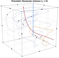
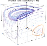
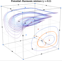
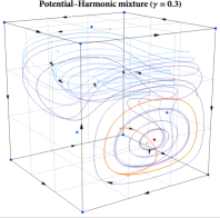
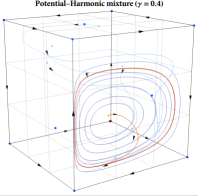
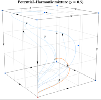
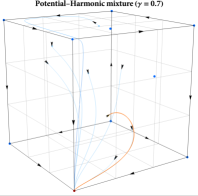
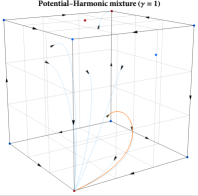
Figure 6. Replicator trajectories in an ensemble of $2\times 2\times 2$ games with payoff $u\coloneqq\gamma u_{p}+(1-\gamma)u_{h}$ given by the convex combination of a harmonic and a potential game. The value of the parameter $\gamma$ is shown in the legend of each plot, and $u_{p},u_{h}$ are given in Section E.2. Each trajectory is color-coded so that deeper shades of blue-purple correspond to later times, with the arrows indicating the direction in which orbits are traversed. Light blue markers represent initial points for the orbits; dark blue markers are stationary points for the replicator dynamics; and dark red points are Nash equilibria. For visual clarity, we have highlighted in orange one of the plotted orbits. As expected, RD is recurrent (in particular, periodic) in the harmonic case $\gamma=0$, and converges to a pure NE in the potential case $\gamma=1$.

Appendix F A geometric tour

A reader familiar with differential geometry won’t have failed to realize that we have been trying to explain some fundamental geometrical concepts in an intuitive, yet not completely rigorous, way. This is an unavoidable price to pay if we wish to present results to an audience not necessarily familiar with the geometrical theory they rely upon.

For that reader, here is a quick tour about what is going on, that can be safely skipped by anyone not interested in the geometrical intricacies underlying the constructions we presented. A notation aside: as usual, for each $i\in\mathcal{N}$, the index $\alpha_{i}\in\mathcal{A}_{i}$ runs from $0_{i}$ to $m_{i}$ and the index $\mu_{i}\in\tilde{\mathcal{A}}_{i}$ runs from $1_{i}$ to $m_{i}$. It is understood that whenever the index $i$ appears in an equation such equation holds true for all $i\in\mathcal{N}$, unless otherwise specified.

• Each open strategy space $\mathcal{X}^{\circ}_{i}=\operatorname{\operatorname{\Delta}}^{\!\circ}(\mathcal{A}_{i})$ is a smooth submanifold of $\mathbb{R}^{\mathcal{A}_{i}}$ of dimension $m_{i}=A_{i}-1$;

• $\pi_{0}\colon\mathcal{X}^{\circ}_{i}\to\mathcal{C}^{\circ}_{i}$ is a global chart and $\iota_{0}\colon\mathcal{C}^{\circ}_{i}\to\mathcal{X}^{\circ}_{i}$ the corresponding parametrization;

• $\mathcal{X}^{\circ}=\prod_{i}\mathcal{X}^{\circ}_{i}$ has the standard smooth structure of product submanifold in $\mathbb{R}^{\mathcal{A}}=\prod_{i}\mathbb{R}^{\mathcal{A}_{i}}$;

• the differential of the parametrization $d\iota_{0}$ is an isomorphism between $\operatorname{T}\mathcal{C}^{\circ}_{i}=\mathbb{R}^{m_{i}}$ and $\operatorname{T}\mathcal{X}^{\circ}_{i}\subset\mathbb{R}^{m_{i}+1}$ allowing to express the $m_{i}$ basis vectors $\{\tilde{\partial}_{i\mu_{i}}\}_{\mu_{i}\in\{1,\dots,m_{i}\}}$ of $\operatorname{T}\mathcal{X}^{\circ}_{i}$ in the chart $\pi_{0}$ as a linear combination of the $m_{i}+1$ basis vectors $\{\partial_{i\alpha_{i}}\}_{\alpha_{i}\in\{0,\dots,m_{i}\}}$ of $\mathbb{R}^{m_{i}+1}$ in the standard Cartesian frame as

  $$\tilde{\partial}_{i\mu_{i}}=\partial_{i\mu_{i}}-\partial_{i0_{i}}\quad\text{for all }\mu_{i}\in\{1,\dots,m_{i}\}\,.$$

• Analogously, the pull-back of the $m_{i}+1$ basis $1$-forms $\{dx^{i\alpha_{i}}\}_{\alpha_{i}\in\{0,\dots,m_{i}\}}$ in $\mathbb{R}_{++}^{\mathcal{A}_{i}}$ along $\iota_{0}$ in terms of the $m_{i}$ basis $1$-forms $\{d\tilde{x}^{i\mu_{i}}\}_{\mu_{i}\in\{1,\dots,m_{i}\}}$ on $\mathcal{X}^{\circ}_{i}$ gives

  $$dx^{i0_{i}}=-\sum_{\mu_{i}}d\tilde{x}^{i\mu_{i}}\quad\text{and}\quad dx^{i\mu_{i}}=d\tilde{x}^{i\mu_{i}}\quad\text{for all }\mu_{i}\in\{1,\dots,m_{i}\}\,.$$

• Payoff functions $u_{i}\colon\mathcal{X}\to\mathbb{R}$ are actually multilinear functions on the whole $u_{i}\colon\mathbb{R}^{\mathcal{A}}\to\mathbb{R}$;

• each “effective payoff function” $\tilde{u}_{i}$ is the pull-back along the inclusion of $u_{i}$, i.e., a smooth function on $\mathcal{X}^{\circ}_{i}$;

• each payoff field $v_{i}=d_{i}u_{i}$ is a $1$-form on $\mathbb{R}^{\mathcal{A}_{i}}$ and $v=\sum_{i}v_{i}$ is a $1$-form on $\mathbb{R}^{\mathcal{A}}$;

• the “effective payoff field” $\tilde{v}_{i}$ is the pull-back along the inclusion of $v_{i}$, i.e., a $1$-form on $\mathcal{X}^{\circ}_{i}$;

• the ambient Shahshahani metric on $\mathbb{R}^{\mathcal{A}}$,

  $$g(x)=\sum_{i\in\mathcal{N}}\sum_{\alpha_{i}\beta_{i}}\frac{\delta_{\alpha_{i}\beta_{i}}}{x_{i\alpha_{i}}}\,dx^{i\alpha_{i}}\otimes dx^{i\beta_{i}}\,,$$

  is pulled back to the effective Shahshahani metric on $\mathcal{X}^{\circ}$,

  $$\tilde{g}(\tilde{x})=\sum_{i\in\mathcal{N}}\sum_{\mu_{i}\nu_{i}}\left(\frac{\delta_{\mu_{i}\nu_{i}}}{\tilde{x}_{i\mu_{i}}}+\frac{1}{x_{i0_{i}}}\right)\,d\tilde{x}^{i\mu_{i}}\otimes d\tilde{x}^{i\nu_{i}}\,.$$

It is a standard fact in differential geometry [53] that if $\iota:(S,g)\hookrightarrow(M,G)$ is a Riemannian submanifold with metric $g$ induced by the ambient metric $G$, then the sharp isomorphism $\sharp$, the pull-back along the inclusion $\iota^{\ast}$, and the orthogonal projection $P_{G}$ commute, in the sense that $P_{G}(\alpha^{\sharp_{G}})=(\iota^{\ast}\alpha)^{\sharp_{g}}$ is a vector field on $S$ for all $1$-forms $\alpha$ on $M$. With this in place, each replicator field $v^{\sharp}_{i}(x)$ is equivalently

• the orthogonal projection on $\mathcal{X}^{\circ}_{i}$ with respect to the ambient Shahshahani metric of the ambient sharp of the $1$-form $v_{i}$ (this point of view is adopted in Mertikopoulos & Sandholm [61]);

• the sharp with respect to the pull-back metric of the pull-back $1$-form $\tilde{v}_{i}$;

• the individual gradient with respect to the pull-back Shahshahani metric of the pull-back payoff function $\tilde{u}_{i}$.

In our notation $v^{\sharp}_{i}$ is a vector field parallel to $\mathcal{X}^{\circ}$, i.e., a vector field legitimately defined on the whole ambient space $\mathbb{R}^{\mathcal{A}}$ that evaluated at $x\in\mathcal{X}^{\circ}$ gives a vector in the tangent space $\operatorname{T}_{x}\mathcal{X}^{\circ}$ as a linear subspace of $\operatorname{T}_{x}\mathbb{R}^{\mathcal{A}}$, so $v^{\sharp}_{i}$ has $m_{i}+1$ components. On the other hand $\tilde{v}^{\sharp}_{i}$ is a vector field on $\mathcal{X}^{\circ}$ with $m_{i}$ components, well-defined without the need to see $\mathcal{X}^{\circ}$ as an immersed submanifold.

The reason to go through the reduction procedure of the replicator field and the Shahshahani metric is that what matters from a dynamical standpoint is the divergence of $\tilde{v}^{\sharp}$ as a vector field on $\mathcal{X}^{\circ}$, but in general given a vector field $X$ parallel to a Riemannian submanifold $\iota:(S,g)\hookrightarrow(M,G)$ there is not a simple relation between its the divergence with respect to the ambient metric and its divergence with respect to the pull-back metric (in particular, $\operatorname{div}_{g}X\neq(\operatorname{div}_{G}X)\circ\iota$); for details see do Carmo [25, Ch. 6]. This ultimately makes it necessary to compute the effective versions (resp. pulled back and projected) of the metric and the vector field at hand.

References

- Abdou et al. [2022] Abdou, J., Pnevmatikos, N., Scarsini, M., and Venel, X. Decomposition of Games: Some Strategic Considerations. Mathematics of Operations Research, 47(1):176–208, February 2022. ISSN 0364-765X. doi: 10.1287/moor.2021.1123.
- Akin [1979] Akin, E. The Geometry of Population Genetics. Lecture Notes in Biomathematics 31. Springer-Verlag Berlin Heidelberg, 1 edition, 1979. ISBN 978-3-540-09711-2 978-3-642-93128-4.
- Amann & Hofbauer [1985] Amann, E. and Hofbauer, J. Permanence in lotka-volterra and replicator equations. In Ebeling, W. and Peschel, M. (eds.), Lotka-Volterra Approach to Cooperation and Competition in Dynamic Systems. Akademie-Verlag, Berlin, 1985.
- Amari & Nagaoka [2000] Amari, S.-i. and Nagaoka, H. Methods of Information Geometry. American Mathematical Soc., 2000. ISBN 978-0-8218-4302-4.
- Arnold [1989] Arnold, V. I. Mathematical Methods of Classical Mechanics. Number 60 in Graduate Texts in Mathematics. Springer, New York, NY, 2 edition, 1989.
- Arora et al. [2012] Arora, S., Hazan, E., and Kale, S. The multiplicative weights update method: A meta-algorithm and applications. Theory of Computing, 8(1):121–164, 2012.
- Auer et al. [1995] Auer, P., Cesa-Bianchi, N., Freund, Y., and Schapire, R. E. Gambling in a rigged casino: The adversarial multi-armed bandit problem. In Proceedings of the 36th Annual Symposium on Foundations of Computer Science, 1995.
- Auer et al. [2002] Auer, P., Cesa-Bianchi, N., Freund, Y., and Schapire, R. E. The nonstochastic multiarmed bandit problem. SIAM Journal on Computing, 32(1):48–77, 2002.
- Basar & Ho [1974] Basar, T. and Ho, Y.-C. Informational properties of the Nash solutions of two stochastic nonzero-sum games. Journal of Economic Theory, 7(4):370–387, April 1974. ISSN 0022-0531. doi: 10.1016/0022-0531(74)90110-0.
- Bekka et al. [2000] Bekka, M. B., Bekka, M. E. B., and Mayer, M. Ergodic Theory and Topological Dynamics of Group Actions on Homogeneous Spaces, volume 269. Cambridge University Press, 2000.
- Bhatia et al. [2013] Bhatia, H., Norgard, G., Pascucci, V., and Bremer, P.-T. The Helmholtz-Hodge Decomposition—A Survey. IEEE Transactions on Visualization and Computer Graphics, 19(8):1386–1404, August 2013.
- Boone & Piliouras [2019] Boone, V. and Piliouras, G. From Darwin to Poincaré and von Neumann: Recurrence and Cycles in Evolutionary and Algorithmic Game Theory, October 2019.
- Bravo & Mertikopoulos [2017] Bravo, M. and Mertikopoulos, P. On the robustness of learning in games with stochastically perturbed payoff observations. Games and Economic Behavior, 103(John Nash Memorial issue):41–66, May 2017.
- Candogan et al. [2011a] Candogan, O., Menache, I., Ozdaglar, A., and Parrilo, P. A. Flows and decompositions of games: harmonic and potential games. Mathematics of Operations Research, 36(3):474–503, 2011a.
- Candogan et al. [2011b] Candogan, O., Ozdaglar, A., and Parrilo, P. A. Dynamics in Near-Potential Games. 2011b. doi: 10.48550/ARXIV.1107.4386.
- Candogan et al. [2011c] Candogan, O., Ozdaglar, A., and Parrilo, P. A. Learning in near-potential games. In 2011 50th IEEE Conference on Decision and Control and European Control Conference, pp. 2428–2433, December 2011c. doi: 10.1109/CDC.2011.6160867.
- Candogan et al. [2013] Candogan, O., Ozdaglar, A., and Parrilo, P. A. Near-Potential Games: Geometry and Dynamics. ACM Transactions on Economics and Computation, 1(2):11:1–11:32, May 2013. ISSN 2167-8375. doi: 10.1145/2465769.2465776.
- Candogan [2013] Candogan, U. O. Dynamic Strategic Interactions : Analysis and Mechanism Design. Thesis, Massachusetts Institute of Technology, 2013.
- Cheng et al. [2016] Cheng, D., Liu, T., Zhang, K., and Qi, H. On Decomposed Subspaces of Finite Games. IEEE Transactions on Automatic Control, 61(11):3651–3656, November 2016. ISSN 1558-2523. doi: 10.1109/TAC.2016.2525936.
- Cheung & Tao [2020] Cheung, Y. K. and Tao, Y. Chaos of Learning Beyond Zero-sum and Coordination via Game Decompositions. In International Conference on Learning Representations, October 2020.
- Conley [1978] Conley, C. C. Isolated Invariant Set and the Morse Index. American Mathematical Society, Providence, RI, 1978.
- Coucheney et al. [2015] Coucheney, P., Gaujal, B., and Mertikopoulos, P. Penalty-regulated dynamics and robust learning procedures in games. Mathematics of Operations Research, 40(3):611–633, August 2015.
- Cressman et al. [1998] Cressman, R., Morrison, W. G., and Wen, J.-F. On the Evolutionary Dynamics of Crime. The Canadian Journal of Economics / Revue canadienne d’Economique, 31(5):1101–1117, 1998. ISSN 0008-4085. doi: 10.2307/136461.
- de Rham [1984] de Rham, G. Differentiable Manifolds: Forms, Currents, Harmonic Forms. Springer Science & Business Media, 1984.
- do Carmo [1992] do Carmo, M. P. Riemannian Geometry. Birkhäuser Boston, 1 edition, 1992.
- Flokas et al. [2020] Flokas, L., Vlatakis-Gkaragkounis, E. V., Lianeas, T., Mertikopoulos, P., and Piliouras, G. No-regret learning and mixed Nash equilibria: They do not mix. In NeurIPS ’20: Proceedings of the 34th International Conference on Neural Information Processing Systems, 2020.
- Friedman [1991] Friedman, D. Evolutionary games in economics. Econometrica, 59(3):637–666, 1991.
- Fudenberg & Tirole [1991] Fudenberg, D. and Tirole, J. Game Theory. The MIT Press, 1991.
- Hannan [1957] Hannan, J. Approximation to Bayes risk in repeated play. In Dresher, M., Tucker, A. W., and Wolfe, P. (eds.), Contributions to the Theory of Games, Volume III, volume 39 of Annals of Mathematics Studies, pp. 97–139. Princeton University Press, Princeton, NJ, 1957.
- Harper [2009] Harper, M. Information geometry and evolutionary game theory. arXiv preprint arXiv:0911.1383, 2009.
- Hart & Mas-Colell [2003] Hart, S. and Mas-Colell, A. Uncoupled dynamics do not lead to Nash equilibrium. American Economic Review, 93(5):1830–1836, 2003.
- Hart & Mas-Colell [2006] Hart, S. and Mas-Colell, A. Stochastic uncoupled dynamics and Nash equilibrium. Games and Economic Behavior, 57:286–303, 2006.
- Héliou et al. [2017] Héliou, A., Cohen, J., and Mertikopoulos, P. Learning with bandit feedback in potential games. In NIPS ’17: Proceedings of the 31st International Conference on Neural Information Processing Systems, 2017.
- Hodge [1989] Hodge, W. V. D. The Theory and Applications of Harmonic Integrals. CUP Archive, May 1989. ISBN 978-0-521-35881-1.
- Hofbauer [1996] Hofbauer, J. Evolutionary dynamics for bimatrix games: A Hamiltonian system? Journal of Mathematical Biology, 34(5):675, May 1996. ISSN 1432-1416. doi: 10.1007/BF02409754.
- Hofbauer & Schlag [2000] Hofbauer, J. and Schlag, K. H. Sophisticated imitation in cyclic games. Journal of Evolutionary Economics, 10(5):523–543, September 2000. ISSN 1432-1386. doi: 10.1007/s001910000049.
- Hofbauer & Sigmund [1998] Hofbauer, J. and Sigmund, K. Evolutionary Games and Population Dynamics. Cambridge University Press, Cambridge, UK, 1998.
- Hsieh et al. [2020] Hsieh, Y.-G., Iutzeler, F., Malick, J., and Mertikopoulos, P. Explore aggressively, update conservatively: Stochastic extragradient methods with variable stepsize scaling. In NeurIPS ’20: Proceedings of the 34th International Conference on Neural Information Processing Systems, 2020.
- Hsieh et al. [2021] Hsieh, Y.-G., Antonakopoulos, K., and Mertikopoulos, P. Adaptive learning in continuous games: Optimal regret bounds and convergence to Nash equilibrium. In COLT ’21: Proceedings of the 34th Annual Conference on Learning Theory, 2021.
- Hsieh et al. [2022] Hsieh, Y.-G., Antonakopoulos, K., Cevher, V., and Mertikopoulos, P. No-regret learning in games with noisy feedback: Faster rates and adaptivity via learning rate separation. In NeurIPS ’22: Proceedings of the 36th International Conference on Neural Information Processing Systems, 2022.
- Hubbard & Burke Hubbard [2015] Hubbard, J. H. and Burke Hubbard, B. Vector Calculus, Linear Algebra, and Differential Forms: A Unified Approach (5th Edition). Matrix Editions, September 2015.
- Hwang & Rey-Bellet [2020] Hwang, S.-H. and Rey-Bellet, L. Strategic decompositions of normal form games: Zero-sum games and potential games. Games and Economic Behavior, 122:370–390, July 2020. ISSN 0899-8256. doi: 10.1016/j.geb.2020.05.003.
- Jiang et al. [2011] Jiang, X., Lim, L.-H., Yao, Y., and Ye, Y. Statistical ranking and combinatorial Hodge theory. Mathematical Programming, 127(1):203–244, 2011.
- Jost [2017] Jost, J. Riemannian Geometry and Geometric Analysis. Universitext. Springer International Publishing, Cham, 2017.
- Kalai & Kalai [2010] Kalai, A. T. and Kalai, E. Cooperation and competition in strategic games with private information. In Proceedings of the 11th ACM Conference on Electronic Commerce, EC ’10, pp. 345–346, New York, NY, USA, June 2010. Association for Computing Machinery. ISBN 978-1-60558-822-3. doi: 10.1145/1807342.1807397.
- Khalil [2002] Khalil, H. K. Nonlinear Systems. Pearson College Div, Upper Saddle River, N.J, subsequent edizione edition, January 2002. ISBN 978-0-13-067389-3.
- Kimura [1958] Kimura, M. On the change of population fitness by natural selection. Heredity, 12:145–167, 1958.
- Kwon & Mertikopoulos [2017] Kwon, J. and Mertikopoulos, P. A continuous-time approach to online optimization. Journal of Dynamics and Games, 4(2):125–148, April 2017.
- Lahkar & Sandholm [2008] Lahkar, R. and Sandholm, W. H. The projection dynamic and the geometry of population games. Games and Economic Behavior, 64:565–590, 2008.
- Laraki & Mertikopoulos [2013] Laraki, R. and Mertikopoulos, P. Higher order game dynamics. Journal of Economic Theory, 148(6):2666–2695, November 2013.
- Laraki & Mertikopoulos [2015] Laraki, R. and Mertikopoulos, P. Inertial game dynamics and applications to constrained optimization. SIAM Journal on Control and Optimization, 53(5):3141–3170, October 2015.
- Lattimore & Szepesvári [2020] Lattimore, T. and Szepesvári, C. Bandit Algorithms. Cambridge University Press, Cambridge, UK, 2020.
- Lee [2012] Lee, J. M. Introduction to Smooth Manifolds. Graduate Texts in Mathematics. Springer-Verlag New York, 2 edition, 2012.
- Lee [2018] Lee, J. M. Introduction to Riemannian Manifolds, volume 176 of Graduate Texts in Mathematics. Springer International Publishing, Cham, 2018. ISBN 978-3-319-91754-2 978-3-319-91755-9. doi: 10.1007/978-3-319-91755-9.
- Letcher et al. [2019] Letcher, A., Balduzzi, D., Racanière, S., Martens, J., Foerster, J., Tuyls, K., and Graepel, T. Differentiable Game Mechanics. Journal of Machine Learning Research, 20(84):1–40, 2019. ISSN 1533-7928.
- Li et al. [2016] Li, C., Liu, T., He, F., Cheng, D., Qi, H., and Hong, Y. On finite harmonic games. In 2016 IEEE 55th Conference on Decision and Control (CDC), pp. 7024–7029, December 2016. doi: 10.1109/CDC.2016.7799351.
- Li et al. [2019] Li, C., Cheng, D., and He, F. A Note On Orthogonal Decomposition of Finite Games, May 2019.
- Littlestone & Warmuth [1994] Littlestone, N. and Warmuth, M. K. The weighted majority algorithm. Information and Computation, 108(2):212–261, 1994.
- Mertikopoulos & Moustakas [2010] Mertikopoulos, P. and Moustakas, A. L. The emergence of rational behavior in the presence of stochastic perturbations. The Annals of Applied Probability, 20(4):1359–1388, July 2010.
- Mertikopoulos & Sandholm [2016] Mertikopoulos, P. and Sandholm, W. H. Learning in games via reinforcement and regularization. Mathematics of Operations Research, 41(4):1297–1324, 2016.
- Mertikopoulos & Sandholm [2018] Mertikopoulos, P. and Sandholm, W. H. Riemannian game dynamics. Journal of Economic Theory, 177:315–364, 2018.
- Mertikopoulos & Zhou [2019] Mertikopoulos, P. and Zhou, Z. Learning in games with continuous action sets and unknown payoff functions. Mathematical Programming, 173(1-2):465–507, January 2019.
- Mertikopoulos et al. [2018] Mertikopoulos, P., Papadimitriou, C. H., and Piliouras, G. Cycles in adversarial regularized learning. In SODA ’18: Proceedings of the 29th annual ACM-SIAM Symposium on Discrete Algorithms, 2018.
- Mertikopoulos et al. [2019] Mertikopoulos, P., Lecouat, B., Zenati, H., Foo, C.-S., Chandrasekhar, V., and Piliouras, G. Optimistic mirror descent in saddle-point problems: Going the extra (gradient) mile. In ICLR ’19: Proceedings of the 2019 International Conference on Learning Representations, 2019.
- Mladenovic et al. [2021] Mladenovic, A., Sakos, I., Gidel, G., and Piliouras, G. Generalized natural gradient flows in hidden convex-concave games and gans. 2021.
- Monderer & Shapley [1996] Monderer, D. and Shapley, L. S. Potential games. Games and Economic Behavior, 14(1):124 – 143, 1996.
- Munkres [1999] Munkres, J. R. Topology. Pearson Higher Ed, 1999.
- Nagarajan et al. [2020] Nagarajan, S. G., Balduzzi, D., and Piliouras, G. From Chaos to Order: Symmetry and Conservation Laws in Game Dynamics. In Proceedings of the 37th International Conference on Machine Learning, pp. 7186–7196. PMLR, November 2020.
- Piliouras & Shamma [2014] Piliouras, G. and Shamma, J. S. Optimization despite chaos: Convex relaxations to complex limit sets via Poincaré recurrence. In SODA ’14: Proceedings of the 25th annual ACM-SIAM Symposium on Discrete Algorithms, 2014.
- Poincaré [1889] Poincaré, H. Sur Le Problème Des Trois Corps et Les Équations de La Dynamique. Mémoire couronné du prix de SM le Roi Oscar II, 1889.
- Rakhlin & Sridharan [2013] Rakhlin, A. and Sridharan, K. Optimization, learning, and games with predictable sequences. In NIPS ’13: Proceedings of the 27th International Conference on Neural Information Processing Systems, 2013.
- Ritzberger & Vogelsberger [1990] Ritzberger, K. and Vogelsberger, K. The Nash field. 1990.
- Rosen [1965] Rosen, J. B. Existence and uniqueness of equilibrium points for concave -person games. Econometrica, 33(3):520–534, 1965.
- Sandholm [2010] Sandholm, W. H. Population Games and Evolutionary Dynamics. MIT Press, Cambridge, MA, 2010.
- Shahshahani [1979] Shahshahani, S. M. A New Mathematical Framework for the Study of Linkage and Selection. Number 211 in Memoirs of the American Mathematical Society. American Mathematical Society, Providence, RI, 1979.
- Shalev-Shwartz [2011] Shalev-Shwartz, S. Online learning and online convex optimization. Foundations and Trends in Machine Learning, 4(2):107–194, 2011.
- Shalev-Shwartz & Singer [2006] Shalev-Shwartz, S. and Singer, Y. Convex repeated games and Fenchel duality. In NIPS’ 06: Proceedings of the 19th Annual Conference on Neural Information Processing Systems, pp. 1265–1272. MIT Press, 2006.
- Smith & Hofbauer [1987] Smith, J. M. and Hofbauer, J. The “battle of the sexes”: A genetic model with limit cycle behavior. Theoretical Population Biology, 32(1):1–14, August 1987. ISSN 0040-5809. doi: 10.1016/0040-5809(87)90035-9.
- Sorin [2009] Sorin, S. Exponential weight algorithm in continuous time. Mathematical Programming, 116(1):513–528, 2009.
- Spivak [1965] Spivak, M. Calculus On Manifolds: A Modern Approach To Classical Theorems Of Advanced Calculus. CRC Press, Boca Raton, 1965. ISBN 978-0-429-50190-6. doi: 10.1201/9780429501906.
- Taylor & Jonker [1978] Taylor, P. D. and Jonker, L. B. Evolutionary stable strategies and game dynamics. Mathematical Biosciences, 40(1-2):145–156, 1978.
- Viossat & Zapechelnyuk [2013] Viossat, Y. and Zapechelnyuk, A. No-regret dynamics and fictitious play. Journal of Economic Theory, 148(2):825–842, March 2013.
- Vovk [1990] Vovk, V. G. Aggregating strategies. In COLT ’90: Proceedings of the 3rd Workshop on Computational Learning Theory, pp. 371–383, 1990.
- Wang et al. [2017] Wang, Y., Liu, T., and Cheng, D. From weighted potential game to weighted harmonic game. IET Control Theory & Applications, 11(13):2161–2169, 2017. ISSN 1751-8652. doi: 10.1049/iet-cta.2016.1454.
- Wei et al. [2021] Wei, C.-Y., Lee, C.-W., Zhang, M., and Luo, H. Linear last-iterate convergence in constrained saddle-point optimization. In ICLR ’21: Proceedings of the 2021 International Conference on Learning Representations, 2021.
- Weibull [1995] Weibull, J. W. Evolutionary Game Theory. MIT Press, Cambridge, MA, 1995.