On Discovery of Local Independence over Continuous Variables
via Neural Contextual Decomposition

Abstract

Conditional independence provides a way to understand causal relationships among the variables of interest. An underlying system may exhibit more fine-grained causal relationships especially between a variable and its parents, which will be called the local independence relationships. One of the most widely studied local relationships is Context-Specific Independence (CSI), which holds in a specific assignment of conditioned variables. However, its applicability is often limited since it does not allow continuous variables: data conditioned to the specific value of a continuous variable contains few instances, if not none, making it infeasible to test independence. In this work, we define and characterize the local independence relationship that holds in a specific set of joint assignments of parental variables, which we call context-set specific independence (CSSI). We then provide a canonical representation of CSSI and prove its fundamental properties. Based on our theoretical findings, we cast the problem of discovering multiple CSSI relationships in a system as finding a partition of the joint outcome space. Finally, we propose a novel method, coined neural contextual decomposition (NCD), which learns such partition by imposing each set to induce CSSI via modeling a conditional distribution. We empirically demonstrate that the proposed method successfully discovers the ground truth local independence relationships in both synthetic dataset and complex system reflecting the real-world physical dynamics.

1 Introduction

Discovering the causal relationships in a system is an important and challenging problem in many areas of scientific research such as social science (Sobel, 1995), biology (Shipley, 2016), and economics (Angrist et al., 1996; Angrist and Pischke, 2008; Imbens and Rubin, 2015; Banerjee et al., 2016; Imbens, 2020). There have been many causal discovery algorithms finding causal relationships given observational data (Spirtes et al., 2000; Chickering, 2002; Hoyer et al., 2008; Shimizu et al., 2006; Zhang et al., 2011; Zheng et al., 2018; Zhu et al., 2019). These methods often exploit conditional independence either explicitly (constraint-based methods) or implicitly (score-based or gradient-based).

A system often exhibits more fine-grained relationships between a variable and its parents, i.e., a local independence relationship. For example, when pushing an object on the ground, it will move only when a force exceeds the friction which is determined by the mass and the ground. Context-specific independence (CSI) (Poole and Zhang, 2003; Boutilier et al., 2013) is the independence that holds in a certain conditioning value (i.e., context) as opposed to any value of the conditioned variables. It has been shown that such independence leads to more efficient probabilistic inference by exploiting the underlying local structure (Poole, 1998; Poole and Zhang, 2003; Gogate and Domingos, 2010; Van den Broeck et al., 2011; Dal et al., 2018). Further, it allows the identification of causal effects, which would not be possible without CSI relationships (Tikka et al., 2019; Robins et al., 2020).

Despite the fact that many real-world scenarios involve continuous variables, most prior works on local independence relationships assumed that variables are discrete. This is partly due to the notion of CSI that is inherently suited for discrete variables as conditioning on the specific value of a continuous variable is infeasible, where the resulting subset of data would be practically empty. Hence, it is non-trivial to explore how local independence for continuous variables can be empirically discovered and utilized in probabilistic or causal inferential tasks.

Consider a system as an example consisting of three observed variables $X_{1}$, $X_{2}$, $Y$, and an unobserved one $U$. We describe the system using a structural causal model (SCM) (Pearl, 2009; Peters et al., 2017). Let $X_{1},X_{2}$ follow a uniform distribution between 0 and 1, and $U$ follow a standard Gaussian distribution. Further, let $Y$ be determined as $Y=X_{1}+U$ if $X_{1}X_{2}<\nicefrac{{1}}{{2}}$ and $Y=X_{2}+U$ otherwise. Focusing on the observable variables, while $Y$ depends on both $X_{1}$ and $X_{2}$ overall (Fig. 1), $Y$ depends only (i) on $X_{1}$ under a certain condition and (ii) on $X_{2}$, otherwise. Since $X_{1}<\nicefrac{{1}}{{2}}$ implies the condition $X_{1}X_{2}<\nicefrac{{1}}{{2}}$ and $Y$ being the function of $X_{1}$ and $U$, it can be represented as CSI (Fig. 1). On the other hand, CSI cannot capture the other local independence where $Y$ is determined only by $X_{2}$ and $U$ since $Y$ and $X_{1}$ are always dependent given any assignment of $X_{2}$.

[] [] []

Figure 1: (a) Causal graph in Example 3.2. (b, c) CSI can represent the local independence of $Y$ and $X_{2}$, but not the other. In contrast, CSSI is able to represent both. (d) Augmented causal graph with PIV $Z$ added in Example D.2. (e, f) PIV representing CSSIs for each context set.

Against this background, we define context-set specific independence (CSSI), a generalized notion of local independence where conditional independence holds in a certain context set, a set of joint assignments of the variables. We characterize context-set specific independence in order to uncover CSSIs for continuous variables, which is more challenging due to an infinite number of context sets. Our characterization leads to the design of NCD (Neural Contextual Decomposition) to find the partitions of the joint outcome space where each partition set induces a CSSI. Our approach is based on approximating a conditional distribution for each partition given a subset of parents. For instance, based on the above example, our method learns two partitions of the Cartesian product of the domains of $X_{1}$ and $X_{2}$, where each partition is flexibly modeled as $\hat{P}(Y|X_{1})$ and $\hat{P}(Y|X_{2})$.

Our contributions are summarized as follows. (i) We introduce the notion of context-set specific independence (CSSI), a new class of local conditional independence relationships. This generalizes two well-known local independence, CSI and partial conditional independence (PCI), and permits continuous conditioned variables. (ii) We characterize context-set specific independence by relating possible CSSIs arisen from a given distribution. We examine a canonical representation of CSSIs and provide a sufficient condition under which a unique CSSIs exists. These characterizations lead to defining contextual decomposition, a way to understand an entire group of CSSIs presenting in a given dataset. (iii) We devise neural contextual decomposition, a simple and effective method for finding a contextual decomposition without directly testing for individual local independence. It utilizes an auxiliary variable (partition indicator variable) used for training of a neural network for context decomposition. Empirical evaluations on a synthetic dataset and Spriteworld demonstrate the effectiveness of the proposed method in recovering local independence relationships.

2 Preliminaries

Throughout this paper, we use capital letters for random variables and small letters for their assignments. Bold letters denote the set of random variables or its assignments. Calligraphy letters can be the domain of corresponding variables or complex mathematical objects.

2.1 Structural Causal Model

We adopt a structural causal model (SCM) (Pearl, 2009) as a causal framework to understand generated data. An SCM $\mathcal{M}$ is defined as a tuple $\left<\mathbf{V},\mathbf{U},\mathbf{F},P(\mathbf{U})\right>$, where $\mathbf{V}=\{V_{1},\cdots,V_{d}\}$ and $\mathbf{U}$ are a set of endogenous and exogenous variables, respectively. $\mathbf{F}=\{f_{1},\cdots,f_{d}\}$ is a set of functions determining each endogenous variable, i.e., $V_{j}\leftarrow f_{j}(Pa(j),\mathbf{U}_{j})$ where $Pa(j)\subseteq\mathbf{V}\setminus\{V_{j}\}$ is a parent of $V_{j}$ and $\mathbf{U}_{j}\subseteq\mathbf{U}$. We may use variable $V_{i}$ and its index $i$ interchangeably. $\mathcal{V}_{j}$ is the outcome space of each variable $V_{j}$. In this work, we restrict to a Markovian model and assume that an SCM satisfies structural minimality (Pearl, 2009; Peters et al., 2017), which asserts that $j\in Pa(i)$ if and only if there exist two values for $j$ that lead to different values for $i$, i.e., $f_{i}(v_{j},\mathbf{v}_{Pa(i)\setminus\{j\}},\mathbf{u}_{i})\neq f_{i}(v^{\prime}_{j},\mathbf{v}_{Pa(i)\setminus\{j\}},\mathbf{u}_{i})$ where $v_{j},v^{\prime}_{j}\in\mathcal{V}_{j}$ and $\mathbf{v}_{Pa(i)\setminus\{j\}}\in\mathcal{V}_{Pa(i)\setminus\{j\}}$. An SCM $\mathcal{M}$ induces a causal graph $\mathcal{G}=(\mathbf{V},\mathbf{E})$, which is a directed acyclic graph (DAG), where $\mathbf{V}=\{1,\ldots,d\}$ and $\mathbf{E}\subseteq\mathbf{V}\times\mathbf{V}$ are the set of nodes and edges, respectively. If $i\in Pa(j)$ in $\mathcal{M}$, then a directed edge $(i,j)$ is in $\mathbf{E}$. In the language of SCM, each node $i$ corresponds to a random variable $V_{i}$ and each edge $(i,j)$ denotes a direct causal relationship from $V_{i}$ to $V_{j}$.

2.2 Local Independence Relationship of Discrete Variables

As described earlier, in many cases, the causal mechanism exhibits fine-grained independence relationships, which do not hold in general but only under certain conditions, i.e., local independence. To begin with, we first provide the definition of context-specific independence (CSI) and partial conditional independence (PCI). We adopt the definitions of CSI and PCI from prior works (Boutilier et al., 2013; Pensar et al., 2015, 2016) for the relationship between a variable and its parents. For the definitions of CSI and PCI, variables are assumed to be discrete. Let ${\mathbf{X}}$ be a non-empty set of parents of $Y$ and ${\mathbf{X}}_{A},{\mathbf{X}}_{B}$ be non-empty partitions of $\mathbf{X}$, i.e., $\mathbf{X}$ is disjoint union of $\mathbf{X}_{A}$ and $\mathbf{X}_{B}$.

Definition 2.1 (Context-Specific Independence (CSI)).

$Y$ is said to be contextually independent of ${\mathbf{X}}_{B}$ given the context ${\mathbf{X}}_{A}={\mathbf{x}}_{A}$ if $P\left(y\mid{\mathbf{x}}_{A},{\mathbf{x}}_{B}\right)=P\left(y\mid{\mathbf{x}}_{A}\right)$, holds for all $y\in\mathcal{Y}$ and ${\mathbf{x}}_{B}\in\mathcal{X}_{B}$ whenever $P\left({\mathbf{x}}_{A},{\mathbf{x}}_{B}\right)>0$. This will be denoted by $Y\mathchoice{\mathrel{\hbox to0.0pt{$\displaystyle\perp$\hss}\mkern 3.0mu{\displaystyle\perp}}}{\mathrel{\hbox to0.0pt{$\textstyle\perp$\hss}\mkern 3.0mu{\textstyle\perp}}}{\mathrel{\hbox to0.0pt{$\scriptstyle\perp$\hss}\mkern 3.0mu{\scriptstyle\perp}}}{\mathrel{\hbox to0.0pt{$\scriptscriptstyle\perp$\hss}\mkern 3.0mu{\scriptscriptstyle\perp}}}{\mathbf{X}}_{B}\mid{\mathbf{X}}_{A}={\mathbf{x}}_{A}$.

Definition 2.2 (Partial Conditional Independence (PCI)).

$Y$ is said to be partially conditionally independent of ${\mathbf{X}}_{B}$ in the domain $\mathcal{D}_{B}\subseteq\mathcal{X}_{B}$ given the context ${\mathbf{X}}_{A}={\mathbf{x}}_{A}$ if $P\left(y\mid{\mathbf{x}}_{A},{\mathbf{x}}_{B}\right)={P(y\mid{\mathbf{x}}_{A},{\mathbf{x}}^{\prime}_{B})}$, holds for all $y\in\mathcal{Y}$ and ${\mathbf{x}}_{B},{\mathbf{x}}_{B}^{\prime}\in\mathcal{D}_{B}$ whenever $P\left({\mathbf{x}}_{A},{\mathbf{x}}_{B}\right)>0$ and $P({\mathbf{x}}_{A},{\mathbf{x}}^{\prime}_{B})>0$. This will be denoted by $Y\mathchoice{\mathrel{\hbox to0.0pt{$\displaystyle\perp$\hss}\mkern 3.0mu{\displaystyle\perp}}}{\mathrel{\hbox to0.0pt{$\textstyle\perp$\hss}\mkern 3.0mu{\textstyle\perp}}}{\mathrel{\hbox to0.0pt{$\scriptstyle\perp$\hss}\mkern 3.0mu{\scriptstyle\perp}}}{\mathrel{\hbox to0.0pt{$\scriptscriptstyle\perp$\hss}\mkern 3.0mu{\scriptscriptstyle\perp}}}{\mathbf{X}}_{B}\mid\mathcal{D}_{B},{\mathbf{X}}_{A}={\mathbf{x}}_{A}$.

PCI is a more fine-grained notion than CSI and, thus, PCI does not imply CSI: $P(y\mid\mathbf{x}_{A},\mathbf{x}_{B})={P(y\mid\mathbf{x}_{A},\mathbf{x}_{B}^{\prime})}$ for all ${\mathbf{x}}_{B},{\mathbf{x}}_{B}^{\prime}\in\mathcal{D}_{B}$ is not equivalent to $P(y\mid\mathbf{x}_{A},\mathbf{x}_{B})=P(y\mid\mathbf{x}_{A})$. Further discussions of the related works on local independence relationships are provided in Sec. 6 and A.1.

3 Compactly Representing Local Independence of Continuous Variables

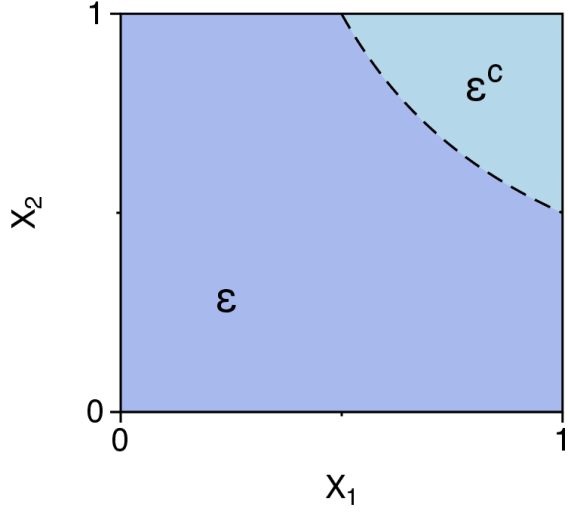
Figure 2: Example 3.2.

Our goal is to find such local independence relationships in a system that may contain continuous variables. The information about local independence relationships of continuous variables can also be leveraged in various tasks as demonstrated in the case of discrete variables. Given that a naive generalization of CSI or PCI to continuous variables seems practically implausible, we first define an alternative notion of local independence, which we call context-set specific independence (CSSI). Then, we characterize CSSI and describe how it can be equipped within the framework of SCM. All omitted proofs can be found in the Appendix.

3.1 Local Independence Relationship over Continuous Variables

Here, we focus on a causal mechanism of a target variable $Y$ and its parents $\mathbf{X}=\{X_{1},\cdots,X_{d}\}$, i.e., SCM $\mathcal{M}=\left<\mathbf{V},\mathbf{U},\mathbf{F},P(\mathbf{U})\right>$ where $\{X_{1},\cdots,X_{d},Y\}\subseteq\mathbf{V}$ is a set of continuous random variables and $Y=f(\mathbf{X},U)$. We denote ${\mathbf{X}}_{A}=\{X_{i}\mid i\in A\}$ where $A\subseteq Pa(Y)=\{1,\cdots,d\}$. Similarly, ${\mathbf{X}}_{A^{c}}=\{X_{i}\mid i\in A^{c}\}$ where $A^{c}=Pa(Y)\setminus A$. Throughout the paper, we assume strictly positive densities. We first define a context-set specific independence (CSSI).

Definition 3.1 (Context-Set Specific Independence).

Let $\mathbf{X}=\{X_{1},\cdots,X_{d}\}$ be a non-empty set of the parents of $Y$ in a causal graph, and ${\mathcal{E}}\subseteq{\mathcal{X}}$ be an event with a positive probability. ${\mathcal{E}}$ is said to be a context set which induces context-set specific independence (CSSI) of $\mathbf{X}_{A^{c}}$ from $Y$ if $p\left(y\mid\mathbf{x}_{A^{c}},\mathbf{x}_{A}\right)=p\left(y\mid\mathbf{x}^{\prime}_{A^{c}},\mathbf{x}_{A}\right)$ holds for every $\left(\mathbf{x}_{A^{c}},\mathbf{x}_{A}\right),\left(\mathbf{x}^{\prime}_{A^{c}},\mathbf{x}_{A}\right)\in{\mathcal{E}}$. This will be denoted by $Y\mathchoice{\mathrel{\hbox to0.0pt{$\displaystyle\perp$\hss}\mkern 3.0mu{\displaystyle\perp}}}{\mathrel{\hbox to0.0pt{$\textstyle\perp$\hss}\mkern 3.0mu{\textstyle\perp}}}{\mathrel{\hbox to0.0pt{$\scriptstyle\perp$\hss}\mkern 3.0mu{\scriptstyle\perp}}}{\mathrel{\hbox to0.0pt{$\scriptscriptstyle\perp$\hss}\mkern 3.0mu{\scriptscriptstyle\perp}}}\mathbf{X}_{A^{c}}\mid\mathbf{X}_{A},{\mathcal{E}}$.

CSSI extends CSI and PCI in the sense that the independence holds in a set of conditioned values in CSSI since they consider a point-based condition. We revisit the earlier example to illustrate how CSI, PCI, and CSSI (Defs 2.1, 2.2 and 3.1) represent the local independence relationships in the system (insufficiency results for CSI and PCI in representing Example 3.2 is depicted in Sec. A.1.)

Example 3.2.

Let $X_{1},X_{2}$ be a uniform random variable defined on $[0,1]$, s.t. $X_{1},X_{2}\sim\textrm{Unif }[0,1]$ and $U$ be an exogenous variable. Let $Y$ be:

$$Y=\begin{cases}X_{1}+U&\text{if }\quad\,\,\,X_{1}X_{2}<\nicefrac{{1}}{{2}},\\ X_{2}+U&\text{if }\quad\,\,\,X_{1}X_{2}\geq\nicefrac{{1}}{{2}}.\end{cases}$$

Let ${\mathcal{E}}=\{(x_{1},x_{2})\mid x_{1}x_{2}<\nicefrac{{1}}{{2}}\}$. Then, $Y\mathchoice{\mathrel{\hbox to0.0pt{$\displaystyle\perp$\hss}\mkern 3.0mu{\displaystyle\perp}}}{\mathrel{\hbox to0.0pt{$\textstyle\perp$\hss}\mkern 3.0mu{\textstyle\perp}}}{\mathrel{\hbox to0.0pt{$\scriptstyle\perp$\hss}\mkern 3.0mu{\scriptstyle\perp}}}{\mathrel{\hbox to0.0pt{$\scriptscriptstyle\perp$\hss}\mkern 3.0mu{\scriptscriptstyle\perp}}}X_{2}\mid X_{1},{\mathcal{E}}$ and $Y\mathchoice{\mathrel{\hbox to0.0pt{$\displaystyle\perp$\hss}\mkern 3.0mu{\displaystyle\perp}}}{\mathrel{\hbox to0.0pt{$\textstyle\perp$\hss}\mkern 3.0mu{\textstyle\perp}}}{\mathrel{\hbox to0.0pt{$\scriptstyle\perp$\hss}\mkern 3.0mu{\scriptstyle\perp}}}{\mathrel{\hbox to0.0pt{$\scriptscriptstyle\perp$\hss}\mkern 3.0mu{\scriptscriptstyle\perp}}}X_{1}\mid X_{2},{\mathcal{E}}^{c}$ hold. On the other hand, $Y\not\mathchoice{\mathrel{\hbox to0.0pt{$\displaystyle\perp$\hss}\mkern 3.0mu{\displaystyle\perp}}}{\mathrel{\hbox to0.0pt{$\textstyle\perp$\hss}\mkern 3.0mu{\textstyle\perp}}}{\mathrel{\hbox to0.0pt{$\scriptstyle\perp$\hss}\mkern 3.0mu{\scriptstyle\perp}}}{\mathrel{\hbox to0.0pt{$\scriptscriptstyle\perp$\hss}\mkern 3.0mu{\scriptscriptstyle\perp}}}X_{1}\mid X_{2}=c$ for any $c$.

As described earlier, we focus on the discovery of local independence (i.e., CSSI) of continuous variables and henceforth assume variables are continuous. In a case where the variables are discrete, CSSI can be discovered by first (i) discovering PCI relationships and then (ii) integrating them (see Sec. A.1 for the detail). We now introduce important properties of CSSI.

Proposition 3.3 (CSSI Entailment)

Suppose a CSSI relationship $Y\mathchoice{\mathrel{\hbox to0.0pt{$\displaystyle\perp$\hss}\mkern 3.0mu{\displaystyle\perp}}}{\mathrel{\hbox to0.0pt{$\textstyle\perp$\hss}\mkern 3.0mu{\textstyle\perp}}}{\mathrel{\hbox to0.0pt{$\scriptstyle\perp$\hss}\mkern 3.0mu{\scriptstyle\perp}}}{\mathrel{\hbox to0.0pt{$\scriptscriptstyle\perp$\hss}\mkern 3.0mu{\scriptscriptstyle\perp}}}\mathbf{X}_{A^{c}}\mid\mathbf{X}_{A},{\mathcal{E}}$ holds. Then, the following CSSI relationships also hold:

(i) $Y\mathchoice{\mathrel{\hbox to0.0pt{$\displaystyle\perp$\hss}\mkern 3.0mu{\displaystyle\perp}}}{\mathrel{\hbox to0.0pt{$\textstyle\perp$\hss}\mkern 3.0mu{\textstyle\perp}}}{\mathrel{\hbox to0.0pt{$\scriptstyle\perp$\hss}\mkern 3.0mu{\scriptstyle\perp}}}{\mathrel{\hbox to0.0pt{$\scriptscriptstyle\perp$\hss}\mkern 3.0mu{\scriptscriptstyle\perp}}}\mathbf{X}_{B^{c}}\mid\mathbf{X}_{B},{\mathcal{E}}\quad$ for any $B\supseteq A$, (ii) $Y\mathchoice{\mathrel{\hbox to0.0pt{$\displaystyle\perp$\hss}\mkern 3.0mu{\displaystyle\perp}}}{\mathrel{\hbox to0.0pt{$\textstyle\perp$\hss}\mkern 3.0mu{\textstyle\perp}}}{\mathrel{\hbox to0.0pt{$\scriptstyle\perp$\hss}\mkern 3.0mu{\scriptstyle\perp}}}{\mathrel{\hbox to0.0pt{$\scriptscriptstyle\perp$\hss}\mkern 3.0mu{\scriptscriptstyle\perp}}}\mathbf{X}_{A^{c}}\mid\mathbf{X}_{A},{\mathcal{F}}\quad$ for any ${\mathcal{F}}\subseteq{\mathcal{E}}$.

Due to such implications, we are interested in CSSI with minimal conditioned variables.

Definition 3.4.

A CSSI of the form $Y\mathchoice{\mathrel{\hbox to0.0pt{$\displaystyle\perp$\hss}\mkern 3.0mu{\displaystyle\perp}}}{\mathrel{\hbox to0.0pt{$\textstyle\perp$\hss}\mkern 3.0mu{\textstyle\perp}}}{\mathrel{\hbox to0.0pt{$\scriptstyle\perp$\hss}\mkern 3.0mu{\scriptstyle\perp}}}{\mathrel{\hbox to0.0pt{$\scriptscriptstyle\perp$\hss}\mkern 3.0mu{\scriptscriptstyle\perp}}}\mathbf{X}_{A^{c}}\mid\mathbf{X}_{A},{\mathcal{E}}$ is said to be regular if there does not exists any $B\subsetneq A$ such that $Y\mathchoice{\mathrel{\hbox to0.0pt{$\displaystyle\perp$\hss}\mkern 3.0mu{\displaystyle\perp}}}{\mathrel{\hbox to0.0pt{$\textstyle\perp$\hss}\mkern 3.0mu{\textstyle\perp}}}{\mathrel{\hbox to0.0pt{$\scriptstyle\perp$\hss}\mkern 3.0mu{\scriptstyle\perp}}}{\mathrel{\hbox to0.0pt{$\scriptscriptstyle\perp$\hss}\mkern 3.0mu{\scriptscriptstyle\perp}}}\mathbf{X}_{B^{c}}\mid\mathbf{X}_{B},{\mathcal{E}}$ holds. Then, we say $\mathbf{X}_{A}$ to be a local parent set of $Y$ in ${\mathcal{E}}$.

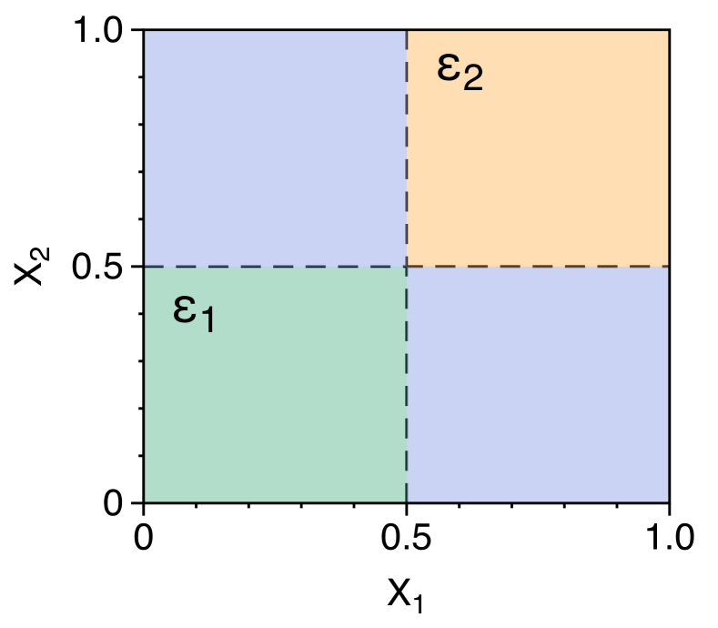
Figure 3: Example 3.5.

Among the CSSIs with the same context set, the regular CSSIs are the most informative, in the sense that the set of the conditioned variables cannot be further reduced. We say a CSSI is trivial if $A=Pa(Y)$ (i.e., $A^{c}=\emptyset$ and ${\mathbf{X}}={\mathbf{X}}_{A}$), since it trivially holds for any ${\mathcal{E}}\subseteq{\mathcal{X}}$. A trivial CSSI on ${\mathcal{E}}={\mathcal{X}}$ is indeed regular. In general, regular CSSI may not be unique on the given context set. We show the non-uniqueness of local parent sets by an example below.

Example 3.5.

Let $X_{1},X_{2},X_{3}\sim\textrm{Unif }[0,1]$ and $U$ be an exogenous variable. Let $Y$ be:

$$Y=\begin{cases}X_{3}+U&\text{if}\quad X_{1},X_{2}<\nicefrac{{1}}{{2}},\\ X_{3}+2\cdot U&\text{if}\quad X_{1},X_{2}\geq\nicefrac{{1}}{{2}},\\ X_{1}+X_{2}+X_{3}+U&\text{otherwise}.\end{cases}$$

Let ${\mathcal{E}}_{1}=\{\mathbf{x}\mid x_{1},x_{2}<\nicefrac{{1}}{{2}}\}$, ${\mathcal{E}}_{2}=\{\mathbf{x}\mid x_{1},x_{2}\geq\nicefrac{{1}}{{2}}\}$. Then, regular CSSIs $Y\mathchoice{\mathrel{\hbox to0.0pt{$\displaystyle\perp$\hss}\mkern 3.0mu{\displaystyle\perp}}}{\mathrel{\hbox to0.0pt{$\textstyle\perp$\hss}\mkern 3.0mu{\textstyle\perp}}}{\mathrel{\hbox to0.0pt{$\scriptstyle\perp$\hss}\mkern 3.0mu{\scriptstyle\perp}}}{\mathrel{\hbox to0.0pt{$\scriptscriptstyle\perp$\hss}\mkern 3.0mu{\scriptscriptstyle\perp}}}X_{12}\mid X_{3},{\mathcal{E}}_{1}$ and $Y\mathchoice{\mathrel{\hbox to0.0pt{$\displaystyle\perp$\hss}\mkern 3.0mu{\displaystyle\perp}}}{\mathrel{\hbox to0.0pt{$\textstyle\perp$\hss}\mkern 3.0mu{\textstyle\perp}}}{\mathrel{\hbox to0.0pt{$\scriptstyle\perp$\hss}\mkern 3.0mu{\scriptstyle\perp}}}{\mathrel{\hbox to0.0pt{$\scriptscriptstyle\perp$\hss}\mkern 3.0mu{\scriptscriptstyle\perp}}}X_{12}\mid X_{3},{\mathcal{E}}_{2}$ hold. Also, the following regular CSSIs hold on ${\mathcal{E}}_{1}\cup{\mathcal{E}}_{2}$:

$$Y\mathchoice{\mathrel{\hbox to0.0pt{$\displaystyle\perp$\hss}\mkern 3.0mu{\displaystyle\perp}}}{\mathrel{\hbox to0.0pt{$\textstyle\perp$\hss}\mkern 3.0mu{\textstyle\perp}}}{\mathrel{\hbox to0.0pt{$\scriptstyle\perp$\hss}\mkern 3.0mu{\scriptstyle\perp}}}{\mathrel{\hbox to0.0pt{$\scriptscriptstyle\perp$\hss}\mkern 3.0mu{\scriptscriptstyle\perp}}}X_{1}\mid X_{23},{\mathcal{E}}_{1}\cup{\mathcal{E}}_{2}\qquad\text{and}\qquad Y\mathchoice{\mathrel{\hbox to0.0pt{$\displaystyle\perp$\hss}\mkern 3.0mu{\displaystyle\perp}}}{\mathrel{\hbox to0.0pt{$\textstyle\perp$\hss}\mkern 3.0mu{\textstyle\perp}}}{\mathrel{\hbox to0.0pt{$\scriptstyle\perp$\hss}\mkern 3.0mu{\scriptstyle\perp}}}{\mathrel{\hbox to0.0pt{$\scriptscriptstyle\perp$\hss}\mkern 3.0mu{\scriptscriptstyle\perp}}}X_{2}\mid X_{13},{\mathcal{E}}_{1}\cup{\mathcal{E}}_{2}.$$

In the example above, there exist two distinct regular CSSIs on ${\mathcal{E}}_{1}\cup{\mathcal{E}}_{2}$. If the local parent set is not unique on the given context set, discovering the local parent set would yield an inconsistent result. Thus, we explore a sufficient condition that guarantees the uniqueness of the local parent set. We now provide an intersection property of CSSI, which will be used to derive a sufficient condition.

Proposition 3.6 (Intersection Property of CSSI)

Suppose ${\mathcal{E}}\subseteq{\mathcal{X}}$ is convex. If CSSI relationships $Y\mathchoice{\mathrel{\hbox to0.0pt{$\displaystyle\perp$\hss}\mkern 3.0mu{\displaystyle\perp}}}{\mathrel{\hbox to0.0pt{$\textstyle\perp$\hss}\mkern 3.0mu{\textstyle\perp}}}{\mathrel{\hbox to0.0pt{$\scriptstyle\perp$\hss}\mkern 3.0mu{\scriptstyle\perp}}}{\mathrel{\hbox to0.0pt{$\scriptscriptstyle\perp$\hss}\mkern 3.0mu{\scriptscriptstyle\perp}}}\mathbf{X}_{A^{c}}\mid\mathbf{X}_{A},{\mathcal{E}}$ and $Y\mathchoice{\mathrel{\hbox to0.0pt{$\displaystyle\perp$\hss}\mkern 3.0mu{\displaystyle\perp}}}{\mathrel{\hbox to0.0pt{$\textstyle\perp$\hss}\mkern 3.0mu{\textstyle\perp}}}{\mathrel{\hbox to0.0pt{$\scriptstyle\perp$\hss}\mkern 3.0mu{\scriptstyle\perp}}}{\mathrel{\hbox to0.0pt{$\scriptscriptstyle\perp$\hss}\mkern 3.0mu{\scriptscriptstyle\perp}}}\mathbf{X}_{B^{c}}\mid\mathbf{X}_{B},{\mathcal{E}}$ hold, then $Y\mathchoice{\mathrel{\hbox to0.0pt{$\displaystyle\perp$\hss}\mkern 3.0mu{\displaystyle\perp}}}{\mathrel{\hbox to0.0pt{$\textstyle\perp$\hss}\mkern 3.0mu{\textstyle\perp}}}{\mathrel{\hbox to0.0pt{$\scriptstyle\perp$\hss}\mkern 3.0mu{\scriptstyle\perp}}}{\mathrel{\hbox to0.0pt{$\scriptscriptstyle\perp$\hss}\mkern 3.0mu{\scriptscriptstyle\perp}}}\mathbf{X}_{(A\cap B)^{c}}\mid\mathbf{X}_{A\cap B},{\mathcal{E}}$ hold.

In Example 3.5, we cannot derive $Y\mathchoice{\mathrel{\hbox to0.0pt{$\displaystyle\perp$\hss}\mkern 3.0mu{\displaystyle\perp}}}{\mathrel{\hbox to0.0pt{$\textstyle\perp$\hss}\mkern 3.0mu{\textstyle\perp}}}{\mathrel{\hbox to0.0pt{$\scriptstyle\perp$\hss}\mkern 3.0mu{\scriptstyle\perp}}}{\mathrel{\hbox to0.0pt{$\scriptscriptstyle\perp$\hss}\mkern 3.0mu{\scriptscriptstyle\perp}}}X_{12}\mid X_{3},{\mathcal{E}}_{1}\cup{\mathcal{E}}_{2}$ from the two regular CSSIs on ${\mathcal{E}}_{1}\cup{\mathcal{E}}_{2}$ as ${\mathcal{E}}_{1}\cup{\mathcal{E}}_{2}$ is not convex. We now introduce a sufficient condition that guarantees the uniqueness of regular CSSIs given a context set ${\mathcal{E}}$.

Theorem 3.7 (Uniqueness of Local Parent Set).

Suppose ${\mathcal{E}}\subseteq{\mathcal{X}}$ is convex. There exists a unique $A\subseteq Pa(Y)$ such that the regular CSSI relationship $Y\mathchoice{\mathrel{\hbox to0.0pt{$\displaystyle\perp$\hss}\mkern 3.0mu{\displaystyle\perp}}}{\mathrel{\hbox to0.0pt{$\textstyle\perp$\hss}\mkern 3.0mu{\textstyle\perp}}}{\mathrel{\hbox to0.0pt{$\scriptstyle\perp$\hss}\mkern 3.0mu{\scriptstyle\perp}}}{\mathrel{\hbox to0.0pt{$\scriptscriptstyle\perp$\hss}\mkern 3.0mu{\scriptscriptstyle\perp}}}\mathbf{X}_{A^{c}}\mid\mathbf{X}_{A},{\mathcal{E}}$ holds.

Proof 3.8.

Suppose regular CSSIs $Y\mathchoice{\mathrel{\hbox to0.0pt{$\displaystyle\perp$\hss}\mkern 3.0mu{\displaystyle\perp}}}{\mathrel{\hbox to0.0pt{$\textstyle\perp$\hss}\mkern 3.0mu{\textstyle\perp}}}{\mathrel{\hbox to0.0pt{$\scriptstyle\perp$\hss}\mkern 3.0mu{\scriptstyle\perp}}}{\mathrel{\hbox to0.0pt{$\scriptscriptstyle\perp$\hss}\mkern 3.0mu{\scriptscriptstyle\perp}}}\mathbf{X}_{A^{c}}\mid\mathbf{X}_{A},{\mathcal{E}}$ and $Y\mathchoice{\mathrel{\hbox to0.0pt{$\displaystyle\perp$\hss}\mkern 3.0mu{\displaystyle\perp}}}{\mathrel{\hbox to0.0pt{$\textstyle\perp$\hss}\mkern 3.0mu{\textstyle\perp}}}{\mathrel{\hbox to0.0pt{$\scriptstyle\perp$\hss}\mkern 3.0mu{\scriptstyle\perp}}}{\mathrel{\hbox to0.0pt{$\scriptscriptstyle\perp$\hss}\mkern 3.0mu{\scriptscriptstyle\perp}}}\mathbf{X}_{B^{c}}\mid\mathbf{X}_{B},{\mathcal{E}}$ hold for some $A$ and $B$. By 3.6 and the convexity of ${\mathcal{E}}$, $(Y\mathchoice{\mathrel{\hbox to0.0pt{$\displaystyle\perp$\hss}\mkern 3.0mu{\displaystyle\perp}}}{\mathrel{\hbox to0.0pt{$\textstyle\perp$\hss}\mkern 3.0mu{\textstyle\perp}}}{\mathrel{\hbox to0.0pt{$\scriptstyle\perp$\hss}\mkern 3.0mu{\scriptstyle\perp}}}{\mathrel{\hbox to0.0pt{$\scriptscriptstyle\perp$\hss}\mkern 3.0mu{\scriptscriptstyle\perp}}}\mathbf{X}_{(A\cap B)^{c}}\mid\mathbf{X}_{A\cap B},{\mathcal{E}})$ holds true. Due to the minimality (i.e., regular), $A\cap B$ cannot be a proper subset of $A$ nor $B$. Hence, $A=B=A\cap B$.

This implies that one may devise a conditional independence test or causal discovery algorithm to find the (unique) local parent set on the convex subset of data (e.g., a rectangular ${\mathcal{E}}=[a_{1},b_{1}]\times\cdots\times[a_{d},b_{d}]\in\mathbb{R}^{d}$ or a ball ${\mathcal{E}}=\{\mathbf{x}\mid\|\mathbf{x}-\mathbf{x}_{0}\|_{2}\leq r\}$). If the subset of data is non-convex, the local parent set may not be unique, and thus the results may not be valid without any additional assumptions. We provide a more general condition for 3.6 and Thm. 3.7 in Appendix B.

4 Discovering Local Independence Relationships by Learning the Partition

We investigate the representation and discovery of multiple CSSIs in a system. To compactly represent CSSIs, we introduce a decomposition of the parents’ outcome space, where each partition corresponds to a CSSI-inducing context set. Then, we transform the finding of such decomposition as a learning problem involving an auxiliary variable representing the decomposition. Finally, we develop a neural approach to learning the decomposition via the auxiliary variable.

4.1 Representing CSSIs in a System as a Partition

We have seen through examples that a system may exhibit multiple CSSIs. We define a canonical notion of CSSI in order to examine a compact representation of CSSIs.

Definition 4.1.

A CSSI relationship $Y\mathchoice{\mathrel{\hbox to0.0pt{$\displaystyle\perp$\hss}\mkern 3.0mu{\displaystyle\perp}}}{\mathrel{\hbox to0.0pt{$\textstyle\perp$\hss}\mkern 3.0mu{\textstyle\perp}}}{\mathrel{\hbox to0.0pt{$\scriptstyle\perp$\hss}\mkern 3.0mu{\scriptstyle\perp}}}{\mathrel{\hbox to0.0pt{$\scriptscriptstyle\perp$\hss}\mkern 3.0mu{\scriptscriptstyle\perp}}}\mathbf{X}_{A^{c}}\mid\mathbf{X}_{A},{\mathcal{E}}$ is canonical if there does not exists any ${\mathcal{F}}\subseteq{\mathcal{E}}$ such that $Y\mathchoice{\mathrel{\hbox to0.0pt{$\displaystyle\perp$\hss}\mkern 3.0mu{\displaystyle\perp}}}{\mathrel{\hbox to0.0pt{$\textstyle\perp$\hss}\mkern 3.0mu{\textstyle\perp}}}{\mathrel{\hbox to0.0pt{$\scriptstyle\perp$\hss}\mkern 3.0mu{\scriptstyle\perp}}}{\mathrel{\hbox to0.0pt{$\scriptscriptstyle\perp$\hss}\mkern 3.0mu{\scriptscriptstyle\perp}}}\mathbf{X}_{B^{c}}\mid\mathbf{X}_{B},{\mathcal{F}}$ and $B\subsetneq A$.

By definition, the canonicality of a CSSI implies its regularity. Canonical CSSIs are the most fine-grained ones since any subset of the context set also entails the same regular CSSI relationship. In Example 3.5, CSSI relationship $Y\mathchoice{\mathrel{\hbox to0.0pt{$\displaystyle\perp$\hss}\mkern 3.0mu{\displaystyle\perp}}}{\mathrel{\hbox to0.0pt{$\textstyle\perp$\hss}\mkern 3.0mu{\textstyle\perp}}}{\mathrel{\hbox to0.0pt{$\scriptstyle\perp$\hss}\mkern 3.0mu{\scriptstyle\perp}}}{\mathrel{\hbox to0.0pt{$\scriptscriptstyle\perp$\hss}\mkern 3.0mu{\scriptscriptstyle\perp}}}X_{1}\mid X_{23},{\mathcal{E}}_{1}\cup{\mathcal{E}}_{2}$ is regular but not canonical since $Y\mathchoice{\mathrel{\hbox to0.0pt{$\displaystyle\perp$\hss}\mkern 3.0mu{\displaystyle\perp}}}{\mathrel{\hbox to0.0pt{$\textstyle\perp$\hss}\mkern 3.0mu{\textstyle\perp}}}{\mathrel{\hbox to0.0pt{$\scriptstyle\perp$\hss}\mkern 3.0mu{\scriptstyle\perp}}}{\mathrel{\hbox to0.0pt{$\scriptscriptstyle\perp$\hss}\mkern 3.0mu{\scriptscriptstyle\perp}}}X_{12}\mid X_{3},{\mathcal{E}}_{1}$. If a trivial CSSI on ${\mathcal{E}}={\mathcal{X}}$ is canonical, a system does not exhibit any CSSI relationship (e.g., Example D.1 in Appendix D). We now define a compact representation of multiple CSSIs in a system.

Definition 4.2 (Contextual Decomposition).

Let $\{{\mathcal{E}}_{k}\}_{k=0}^{N}$ be a partition of ${\mathcal{X}}$. $\{({\mathcal{E}}_{k},{A_{k}})\}_{k=0}^{N}$ is a contextual decomposition (CD) if regular CSSI $Y\mathchoice{\mathrel{\hbox to0.0pt{$\displaystyle\perp$\hss}\mkern 3.0mu{\displaystyle\perp}}}{\mathrel{\hbox to0.0pt{$\textstyle\perp$\hss}\mkern 3.0mu{\textstyle\perp}}}{\mathrel{\hbox to0.0pt{$\scriptstyle\perp$\hss}\mkern 3.0mu{\scriptstyle\perp}}}{\mathrel{\hbox to0.0pt{$\scriptscriptstyle\perp$\hss}\mkern 3.0mu{\scriptscriptstyle\perp}}}\mathbf{X}_{A_{k}^{c}}\mid\mathbf{X}_{A_{k}},{\mathcal{E}}_{k}$ holds for all $k$ where $A_{0}=Pa(Y)$ and $A_{k}\subsetneq Pa(Y)$ for all $k\geq 1$. We say a CD $\{({\mathcal{E}}_{k},A_{k})\}_{k=0}^{N}$ is canonical if $Y\mathchoice{\mathrel{\hbox to0.0pt{$\displaystyle\perp$\hss}\mkern 3.0mu{\displaystyle\perp}}}{\mathrel{\hbox to0.0pt{$\textstyle\perp$\hss}\mkern 3.0mu{\textstyle\perp}}}{\mathrel{\hbox to0.0pt{$\scriptstyle\perp$\hss}\mkern 3.0mu{\scriptstyle\perp}}}{\mathrel{\hbox to0.0pt{$\scriptscriptstyle\perp$\hss}\mkern 3.0mu{\scriptscriptstyle\perp}}}\mathbf{X}_{A_{k}^{c}}\mid\mathbf{X}_{A_{k}},{\mathcal{E}}_{k}$ is canonical for all $k$, and is distinctive if $A_{i}\neq A_{j}$ for all $i\neq j$.

${\mathcal{E}}_{0}$ is a set to cover a remaining subset of ${\mathcal{X}}$ excluding non-trivial context sets. $({\mathcal{E}}_{0},A_{0})$ corresponds to a trivial CSSI. For any causal system, $\{({\mathcal{X}},Pa(Y))\}$ is a CD, which we call trivial CD. When a system does not exhibit any CSSI relationship, a trivial CD is the only existing CD. In Example 3.5, both $\{({\mathcal{E}}_{0},{\mathbf{X}}_{123}),({\mathcal{E}}_{1},{\mathbf{X}}_{3}),({\mathcal{E}}_{2},{\mathbf{X}}_{3})\}$ and $\{({\mathcal{E}}_{0},{\mathbf{X}}_{123}),({\mathcal{E}}_{1}\cup{\mathcal{E}}_{2},{\mathbf{X}}_{23})\}$ are CDs where ${\mathcal{E}}_{0}=({\mathcal{E}}_{1}\cup{\mathcal{E}}_{2})^{c}$. The former is canonical, but the latter is not. Contextual decomposition can be viewed as the discretization of the joint outcome space, in contrast to discretizing each variable which is a commonly used strategy to handle continuous variables (Nyman et al., 2017). As a canonical CSSI is a fine-grained notion of CSSI relationship, a canonical CD can also be viewed as a fine-grained CD. While a canonical CD may not be unique (e.g., Example D.3 in Appendix D), the following theorem characterizes the shared property of the canonical CDs in a system.

Theorem 4.3.

Let $\{({\mathcal{E}}_{i},A_{i})\}_{i=0}^{N}$ and $\{({\mathcal{F}}_{j},B_{j})\}_{j=0}^{M}$ be canonical CDs where ${\mathcal{E}}_{i}$ and ${\mathcal{F}}_{j}$ are open sets for all $i,j\geq 1$. Then, the following holds: (i) if $p({\mathcal{E}}_{i}\cap{\mathcal{F}}_{j})>0$ then $A_{i}=B_{j}$, and (ii) for any $C\subseteq Pa(Y)$, $p({\mathcal{E}}[C]\bigtriangleup{\mathcal{F}}[C])=0$ where ${\mathcal{E}}[C]=\bigcup_{A_{i}=C}{\mathcal{E}}_{i}$ and ${\mathcal{F}}[C]={\bigcup}_{B_{j}=C}{\mathcal{F}}_{j}$.

Roughly, any intersecting context sets (i.e., $p({\mathcal{E}}_{i}\cap{\mathcal{F}}_{j})>0$) from different canonical CDs share the same local parent set (i.e., $A_{i}=B_{j}$). Also, for any $C\subseteq Pa(Y)$, the union of the context sets having the same local parent set $C$ is identical for any canonical CSSI in a system (i.e., $p({\mathcal{E}}[C]\bigtriangleup{\mathcal{F}}[C])=0$). We provide an example of canonical CDs to elaborate Thm. 4.3 in Example D.3 (Appendix D). An interesting property of CDs is that the union of the context sets having the same local parents set may no longer entail the same one, i.e., $\mathbf{pa}^{{\mathcal{E}}_{1}\cup{\mathcal{E}}_{2}}\neq\mathbf{pa}^{{\mathcal{E}}_{1}}\cup\mathbf{pa}^{{\mathcal{E}}_{2}}$, in general as shown in Example 3.5. For the case of distinctive canonical CDs, we have stronger uniqueness which directly follows from Thm. 4.3.

Corollary 4.4 (Uniqueness of Distinctive Canonical CD)

Let $\{({\mathcal{E}}_{i},A_{i})\}_{i=0}^{N}$ and $\{({\mathcal{F}}_{j},B_{j})\}_{j=0}^{M}$ be distinctive canonical CDs where ${\mathcal{E}}_{i}$ and ${\mathcal{F}}_{j}$ are open sets for all $i,j\geq 1$. Then, the following hold: (i) $N=M$, and (ii) if $p({\mathcal{E}}_{i}\cap{\mathcal{F}}_{j})>0$ then $A_{i}=B_{j}$ and $p({\mathcal{E}}_{i}\bigtriangleup{\mathcal{F}}_{j})=0$.

In words, distinctive canonical CD is unique since any intersecting context sets (i.e., $p({\mathcal{E}}_{i}\cap{\mathcal{F}}_{j})>0$) from different distinctive canonical CDs share the same local parent set (i.e., $A_{i}=B_{j}$), and their difference is negligible (i.e., $p({\mathcal{E}}_{i}\bigtriangleup{\mathcal{F}}_{j})=0$).

4.2 Representing Contextual Decomposition with an Auxiliary Variable

We now introduce a partition indicator variable, which will serve as a mapping between ${\mathcal{X}}$ and an arbitrary contextual decomposition. This variable will be useful in transforming the task of testing for CSSI to the task of learning such decomposition. We first show that a CD can be represented by introducing an auxiliary variable.

Proposition 4.5 (Expressing CSSI as CSI with Auxiliary Variable)

Let $\{{\mathcal{E}}_{k}\}_{k=0}^{N}$ be a partition of $\mathcal{X}$. $\{({\mathcal{E}}_{k},A_{k})\}_{k=0}^{N}$ is a contextual decomposition if and only if $Y\mathchoice{\mathrel{\hbox to0.0pt{$\displaystyle\perp$\hss}\mkern 3.0mu{\displaystyle\perp}}}{\mathrel{\hbox to0.0pt{$\textstyle\perp$\hss}\mkern 3.0mu{\textstyle\perp}}}{\mathrel{\hbox to0.0pt{$\scriptstyle\perp$\hss}\mkern 3.0mu{\scriptstyle\perp}}}{\mathrel{\hbox to0.0pt{$\scriptscriptstyle\perp$\hss}\mkern 3.0mu{\scriptscriptstyle\perp}}}\mathbf{X}_{A_{k}^{c}}\mid\mathbf{X}_{A_{k}},Z=z_{k}$ holds for all $k\geq 1$, where $Z$ is the deterministic random variable defined as $Z=z_{k}$ if $\mathbf{X}\in{\mathcal{E}}_{k}$ for all $k$.

In Example 3.2, we can introduce $Z$ so that $Y\mathchoice{\mathrel{\hbox to0.0pt{$\displaystyle\perp$\hss}\mkern 3.0mu{\displaystyle\perp}}}{\mathrel{\hbox to0.0pt{$\textstyle\perp$\hss}\mkern 3.0mu{\textstyle\perp}}}{\mathrel{\hbox to0.0pt{$\scriptstyle\perp$\hss}\mkern 3.0mu{\scriptstyle\perp}}}{\mathrel{\hbox to0.0pt{$\scriptscriptstyle\perp$\hss}\mkern 3.0mu{\scriptscriptstyle\perp}}}X_{2}\mid X_{1},Z=z_{1}$ and $Y\mathchoice{\mathrel{\hbox to0.0pt{$\displaystyle\perp$\hss}\mkern 3.0mu{\displaystyle\perp}}}{\mathrel{\hbox to0.0pt{$\textstyle\perp$\hss}\mkern 3.0mu{\textstyle\perp}}}{\mathrel{\hbox to0.0pt{$\scriptstyle\perp$\hss}\mkern 3.0mu{\scriptstyle\perp}}}{\mathrel{\hbox to0.0pt{$\scriptscriptstyle\perp$\hss}\mkern 3.0mu{\scriptscriptstyle\perp}}}X_{1}\mid X_{2},Z=z_{2}$ where $Z=z_{1}$ if ${\mathbf{X}}\in{\mathcal{E}}$ and $z_{2}$ otherwise. We now formally define a partition indicator variable.

Definition 4.6.

Let $\{{\mathcal{E}}_{k}\}_{k=0}^{N}$ be a partition of $\mathcal{X}$ and a random variable $Z$ be defined as $Z=z_{k}$ if $\mathbf{X}\in{\mathcal{E}}_{k}$ for all $0\leq k\leq N$. Variable $Z$ is a partition indicator variable (PIV) if for all $k\geq 1$ there exists some $A_{k}\subsetneq Pa(Y)$ such that $Y\mathchoice{\mathrel{\hbox to0.0pt{$\displaystyle\perp$\hss}\mkern 3.0mu{\displaystyle\perp}}}{\mathrel{\hbox to0.0pt{$\textstyle\perp$\hss}\mkern 3.0mu{\textstyle\perp}}}{\mathrel{\hbox to0.0pt{$\scriptstyle\perp$\hss}\mkern 3.0mu{\scriptstyle\perp}}}{\mathrel{\hbox to0.0pt{$\scriptscriptstyle\perp$\hss}\mkern 3.0mu{\scriptscriptstyle\perp}}}\mathbf{X}_{A_{k}^{c}}\mid\mathbf{X}_{A_{k}},Z=z_{k}$.

PIV can be viewed as a particular type of sufficient set of statistics. 4.5 implies that a PIV represents a corresponding CD. With PIV $Z$, each CSSI relationship $Y\mathchoice{\mathrel{\hbox to0.0pt{$\displaystyle\perp$\hss}\mkern 3.0mu{\displaystyle\perp}}}{\mathrel{\hbox to0.0pt{$\textstyle\perp$\hss}\mkern 3.0mu{\textstyle\perp}}}{\mathrel{\hbox to0.0pt{$\scriptstyle\perp$\hss}\mkern 3.0mu{\scriptstyle\perp}}}{\mathrel{\hbox to0.0pt{$\scriptscriptstyle\perp$\hss}\mkern 3.0mu{\scriptscriptstyle\perp}}}\mathbf{X}_{A_{k}^{c}}\mid\mathbf{X}_{A_{k}},{\mathcal{E}}_{k}$ is equivalently expressed as $Y\mathchoice{\mathrel{\hbox to0.0pt{$\displaystyle\perp$\hss}\mkern 3.0mu{\displaystyle\perp}}}{\mathrel{\hbox to0.0pt{$\textstyle\perp$\hss}\mkern 3.0mu{\textstyle\perp}}}{\mathrel{\hbox to0.0pt{$\scriptstyle\perp$\hss}\mkern 3.0mu{\scriptstyle\perp}}}{\mathrel{\hbox to0.0pt{$\scriptscriptstyle\perp$\hss}\mkern 3.0mu{\scriptscriptstyle\perp}}}\mathbf{X}_{A_{k}^{c}}\mid\mathbf{X}_{A_{k}},Z=z_{k}$. Thus, for ${\mathbf{x}}\in{\mathcal{E}}_{k}$,

$$p(y\mid{\mathbf{x}})=p(y\mid{\mathbf{x}},z_{k})=p(y\mid{\mathbf{x}}_{A_{k}^{c}},{\mathbf{x}}_{A_{k}},z_{k})=p(y\mid{\mathbf{x}}_{A_{k}},z_{k}),$$ (1)

where the first equality holds by definition, and the last equality holds since PIV entails CSI relationships. Therefore some of the parent variables (i.e., ${\mathbf{X}}_{A_{k}^{c}}$) would be ignored for modeling the conditional distribution of $Y$ given ${\mathcal{E}}_{k}$. In contrast to CSI, which uses the value of a proper subset of $Pa(Y)$ ignoring the rest, the value of $Z$ is determined by the whole ${\mathbf{X}}$, in general, and a subset of $Pa(Y)$ to be ignored (i.e., ${\mathbf{X}}_{A_{k}^{c}}$) could involve in determining the value of $Z$.

4.3 Neural Contextual Decomposition

As described earlier, conditional independence tests can be used to discover the CSSI relationship on a particular subset of data. Further, assuming strictly positive densities, testing on a convex subset of data is sufficient to obtain a unique local parent set without any additional assumptions. However, it is generally infeasible to test on every possible subset to discover multiple CSSIs in a given system.

Against this background, we propose Neural Contextual Decomposition (NCD), a neural approach to recovering distinct contextual decomposition from given data $P(\mathbf{V})$ via learning PIV $Z$. Recalling $Y\mathchoice{\mathrel{\hbox to0.0pt{$\displaystyle\perp$\hss}\mkern 3.0mu{\displaystyle\perp}}}{\mathrel{\hbox to0.0pt{$\textstyle\perp$\hss}\mkern 3.0mu{\textstyle\perp}}}{\mathrel{\hbox to0.0pt{$\scriptstyle\perp$\hss}\mkern 3.0mu{\scriptstyle\perp}}}{\mathrel{\hbox to0.0pt{$\scriptscriptstyle\perp$\hss}\mkern 3.0mu{\scriptscriptstyle\perp}}}\mathbf{X}_{A_{k}^{c}}\mid\mathbf{X}_{A_{k}},Z=z_{k}$, we let ${\mathcal{Z}}\subseteq\{0,1\}^{d}$ so that the local parent set $A_{k}$ corresponds to the set of the indices of the nonzero element of $z_{k}$, e.g., $Y\mathchoice{\mathrel{\hbox to0.0pt{$\displaystyle\perp$\hss}\mkern 3.0mu{\displaystyle\perp}}}{\mathrel{\hbox to0.0pt{$\textstyle\perp$\hss}\mkern 3.0mu{\textstyle\perp}}}{\mathrel{\hbox to0.0pt{$\scriptstyle\perp$\hss}\mkern 3.0mu{\scriptstyle\perp}}}{\mathrel{\hbox to0.0pt{$\scriptscriptstyle\perp$\hss}\mkern 3.0mu{\scriptscriptstyle\perp}}}X_{2}\mid X_{13},Z=(1,0,1)$. With PIV $Z$, we can write the conditional density as:

$$\textstyle{p(y\mid{\mathbf{x}})=\sum_{z}p(y\mid{\mathbf{x}},z)p(z\mid{\mathbf{x}})=\sum_{z}p(y\mid{\mathbf{x}}_{A_{z}},z)p(z\mid{\mathbf{x}}),}$$ (2)

where $A_{z}$ is $A_{k}$ corresponding to $z_{k}$ and $p(z\mid{\mathbf{x}})=\delta(z=z_{i})$ if ${\mathbf{x}}\in{\mathcal{E}}_{i}$. Our method models $p(y\mid{\mathbf{x}},z)$ and $p(z\mid{\mathbf{x}})$.

Modeling $p(y\mid{\mathbf{x}},z)$ and $p(z\mid{\mathbf{x}})$.

Since $p(y\mid{\mathbf{x}},z)=p(y\mid{\mathbf{x}}_{A_{z}},z)$, some of the parent variables (i.e., ${\mathbf{x}}_{A_{z}^{c}}$) are redundant for modeling a conditional distribution. Therefore, our method approximates the conditional distribution $p(y\mid{\mathbf{x}},z)$ as $\hat{p}(y\mid{\mathbf{x}},z)$ and let a neural network $f_{\theta}$ takes $(\mathbf{x}\odot z,z)$ as an input where $\odot$ denotes an element-wise product and outputs the parameters of the estimator $\hat{p}(y\mid\mathbf{x},z)$. For the input of $f_{\theta}$, we simply concatenate ${\mathbf{x}}\odot z$ and $z$, e.g., if $z=(1,0,1)$ then $f_{\theta}$ takes $({\mathbf{x}}\odot z,z)=(x_{1},0,x_{3},1,0,1)$ as an input. We emphasize that labeling (i.e., concatenation of $z$) is essential since ${\mathbf{x}}_{A_{k}^{c}}$ cannot be ignored without conditioning on $z$, i.e., $p(y\mid{\mathbf{x}})=p(y\mid{\mathbf{x}},z_{k})=p(y\mid{\mathbf{x}}_{A_{k}},z_{k})$ holds for ${\mathbf{x}}\in{\mathcal{E}}_{k}$ but $p(y\mid{\mathbf{x}})\neq p(y\mid{\mathbf{x}}_{A_{k}})$ and $p(y\mid{\mathbf{x}},z_{k})\neq p(y\mid{\mathbf{x}}_{A_{k}})$ in general. Moreover, without labeling, it is unable to distinguish whether the zero entries of input are either masked or its assignment being zero. We also model the conditional distribution $p(z\mid{\mathbf{x}})$ as $\hat{p}(z\mid{\mathbf{x}})$, and let a neural network $g_{\phi}$ takes ${\mathbf{x}}$ as input and outputs the parameters of Bernoulli variables. That is, $g_{\phi}({\mathbf{x}})=(\pi_{1},\cdots,\pi_{d})$ and $z_{(k)}|{\mathbf{x}}\sim\text{Bernoulli}(\pi_{k})$ for all $k$ where $z=(z_{(1)},\cdots,z_{(d)})\in\{0,1\}^{d}$. We provide further discussions of the related works on neural network based causal discovery methods in Sec. 6.

Training objective.

Our model becomes $p(y\mid{\mathbf{x}};\theta,\phi)={\sum_{z}\hat{p}(y\mid{\mathbf{x}},z)\hat{p}(z\mid{\mathbf{x}})}={\mathbb{E}_{\hat{p}(z\mid{\mathbf{x}})}\hat{p}(y\mid{\mathbf{x}},z)}$, and its maximum likelihood estimation is as follows:

$$\sup_{\theta,\phi}\,\mathbb{E}_{p({\mathbf{x}},y)}\big{[}\log\,\mathbb{E}_{\hat{p}(z\mid{\mathbf{x}})}\,\hat{p}(y\mid{\mathbf{x}},z)\big{]}.$$ (3)

For the inner expectation, we use the Monte Carlo approximation: $\frac{1}{N}\sum_{i=1}^{N}\hat{p}(y\mid{\mathbf{x}},z^{(i)})$, where $z^{(i)}\sim\hat{p}(z\mid{\mathbf{x}})$. We also use Gumbel-Softmax estimator (Jang et al., 2016; Maddison et al., 2016) to enable the learning with neural networks. The final training objective is as follows:

$$\mathcal{L}(\theta,\phi;\mathcal{D})={\sum}_{(\mathbf{x},y)\in\mathcal{D}}\big{(}\log\frac{1}{N}\sum_{i=1}^{N}\hat{p}(y\mid{\mathbf{x}},z^{(i)})\big{)},$$ (4)

where $z^{(i)}$ is sampled from $\hat{p}(z\mid{\mathbf{x}})$ and $\mathcal{D}$ is a dataset of samples, which could be a minibatch in practice, from the joint distribution entailed by an underlying SCM. Further details of the implementation of NCD are provided in Sec. E.3.

5 Empirical Evaluation

In this section, we evaluate our proposed method to discover contextual decomposition and CSSIs. We first consider causal systems with different types of functional model and varying complexity of partition (Sec. 5.1), and then a more complex system reflecting the real-world physical dynamics (Sec. 5.2).

We compare our method with attention-based methods (Pitis et al., 2020) which aims to discover the local structure in a causal system of continuous variables, by computing the attention weights of the input ${\mathbf{x}}$. It first trains a transformer (Vaswani et al., 2017) to model the conditional distribution $p(y\mid{\mathbf{x}})$. Then, it uses the attention weights $(a_{1},\cdots,a_{d})$ of the input ${\mathbf{x}}$ to discover the local independence relationship. Intuitively, a low attention score $a_{j}$ implies that the input variable $X_{j}$ has a weak influence on the target variable $Y$. We also compare with a mixture model, which applies a single attention layer on top of the multiple NNs. Local independence is discovered by first computing the approximation of the Jacobian of each NNs and then applying the weighted sum with the learned attention score. For the experiments on the synthetic dataset, we let the number of the NNs be equal to the ground truth number of partition sets (i.e., oracle modeling).

For the implementation of $f_{\theta}({\mathbf{x}}\odot z,z)$, which outputs the parameters of the Gaussian distribution $\hat{p}(y\mid{\mathbf{x}},z)$, and $g_{\phi}({\mathbf{x}})$, which outputs the parameters of the Bernoulli distributions, we used MLPs with 3 hidden layers and hidden units of 128. For all experiments, we set the batch size to 1000 and trained our method and the baselines for 100 epochs. All of our experiments were conducted with 3 different seeds, and a shaded area in a ROC plot represents a standard deviation. A detailed description of the baseline methods and further implementation details are provided in Sec. E.3.

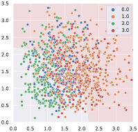
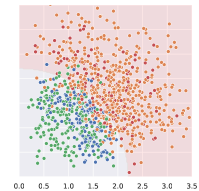
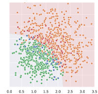
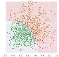
Figure 4: Learned decision boundaries (partition) for epochs 5, 10, 15, and 20. Labels 0, 1, 2, and 3 denote $z=(0,0),(0,1),(1,0)$, and $(1,1)$, respectively.

5.1 Synthetic Data

We consider causal systems where distinctive CD exists. We generate synthetic datasets consisting of the samples $({\mathbf{X}},Y)$ where ${\mathbf{X}}=\{X_{1},\cdots,X_{d}\}$ is the parent variables of $Y$. We assume the parent variables are independent and follow the unit normal. The data generating process is as follows:

$$Y=f_{i}(\mathbf{X}_{A_{i}},U)\quad\text{if }\quad\mathbf{x}\in{\mathcal{E}}_{i},\quad\text{for }\quad 0\leq i\leq N,$$ (5)

where $U$ is an exogenous variable, $\{{\mathcal{E}}_{k}\}_{k=0}^{N}$ is a partition of $\mathcal{X}$, $A_{i}$ is distinctive to each other (i.e., $A_{i}\neq A_{j}$ for all $i\neq j$). In our experiments, $d=9$ and the exogenous variable follows the unit normal. We evaluate our method with varying types of functions $f_{k}$, local parents sets $A_{k}$, and partition sets ${\mathcal{E}}_{k}$. For the functions $\{f_{k}\}$, we consider nonlinear functions with (i) additive and (ii) non-additive noise models. We use randomly initialized neural networks for the nonlinear functions, i.e., we do not assume any specific family of distributions for $f_{k}$. For the partition $\{{\mathcal{E}}_{k}\}$, we consider the cases where the boundaries of the partition sets are (i) linear and (ii) nonlinear. In the case of linear boundaries, partition sets are defined by a linear function $h$, i.e., $x\in{\mathcal{E}}_{k}$ if $h({\mathbf{X}}_{A_{k}})=\text{max}(h({\mathbf{X}}_{A_{0}}),\cdots,h({\mathbf{X}}_{A_{N}}))$. For the nonlinear boundaries, we further control the complexity of the partition by considering both cases when nonlinear boundaries are determined by the norm of ${\mathbf{x}}$ and some nonlinear function $h$. For the local parent sets $\{{\mathbf{X}}_{A_{0}},{\mathbf{X}}_{A_{1}},{\mathbf{X}}_{A_{2}}\}$, we consider two cases: (i) uniformly distributed as $\{{\mathbf{X}}_{123},{\mathbf{X}}_{456},{\mathbf{X}}_{789}\}$ and (ii) non-uniformly distributed as $\{{\mathbf{X}},{\mathbf{X}}_{123},{\mathbf{X}}_{456789}\}$. In our experiments, we use different configurations of functions, local parent sets, and boundaries. For the main experiments, we consider the case of nonlinear functions with a non-additive noise model and report the results under the additive noise model in the appendix. We provide the details of the setups and implementations in Sec. E.1.

Experimental results.

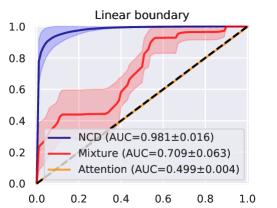
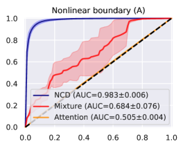
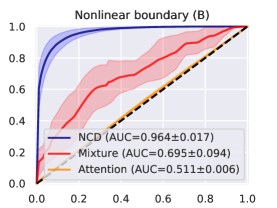
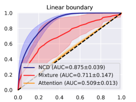
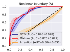
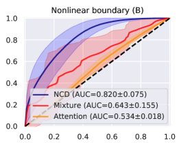
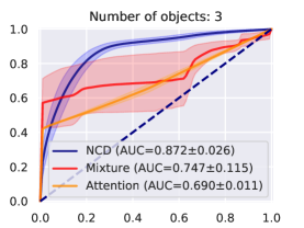
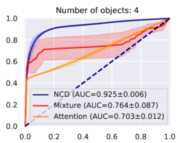
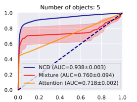
Figure 5: ROC curves for the ground truth local independence relationships on (top, middle) the synthetic dataset of (top) uniformly and (middle) non-uniformly distributed local parent sets with different types of boundaries and (bottom) on the Spriteworld.

We illustrate our results in Fig. 5 for (top) the uniformly and (middle) non-uniformly distributed local parent sets, respectively. Our method successfully discovers local independence structures and outperforms the baselines in most cases. We again emphasize that the mixture model exploits the ground truth number of partition sets for its implementation.

Visualization of the predicted partition.

We present plots in Fig. 4 illustrating how the neural network learns the partition throughout the training procedure based on a toy experiment with 2 parent variables $\mathbf{X}=\{X_{1},X_{2}\}$. The quality of the discovered contextual decomposition is improved as the training goes on. Our model successfully discovered the local independence and the corresponding context sets. It shows that the data points within each partition are properly classified, while the model fails to classify some points close to the decision boundary.

5.2 Complex System Reflecting Real-world Dynamics

We examine our method on the modified Spriteworld environment (Watters et al., 2019; Pitis et al., 2020), which reflects real-world physics dynamics, to evaluate our method in a more complex environment. In a 2 dimensional space, there are $n$ moving objects (i.e., sprites), which can collide with each other. Each $i$-th object corresponds to two 2-dimensional variables $X_{2i-1}=(x,y)_{(i)},X_{2i}=(v_{x},v_{y})_{(i)}$ which represents the position and the velocity of the object. An agent can influence the objects through an action. Action corresponds to a 2-dimensional variable $X_{2n+1}=(a_{x},a_{y})$, representing some position in the 2D scene, and it influences the dynamics of the nearest object, thus there are interactions between the action and each object. In each time-step, the object and action variables influence the object variables of the next time-step. Formally, ${\mathbf{X}}=\{X_{1},\cdots,X_{2n+1}\}$ and ${\mathbf{Y}}=\{Y_{1},\cdots,Y_{2n}\}$ where ${\mathbf{X}}$ denotes the object and action variables and ${\mathbf{Y}}$ denotes the object variables of the next time-step. Further, there exist dependencies among the parent variables. Each $Y_{k}$ is generated from ${\mathbf{X}}$ with an unknown dynamics function $f_{k}$, i.e., $Y_{k}=f_{k}({\mathbf{X}},U)$ where $U$ is the exogenous variable. As a whole, all ${\mathbf{X}}$ are involved in generating each $Y_{k}$ since the objects can collide with each other and the action influences the objects. However, the interactions are sparse—the collision occurs only when objects are (i) close enough and (ii) heading toward each other. Thus, the dynamics system exhibits numerous CSSI relationships. As shown in the bottom of Fig. 5, our method recovers the ground truth local structure on the varying number of objects. We provide further details of the dataset and the implementation in Sec. E.2.

6 Related Work

Local independence relationship.

One of the most widely used local independence relationships is the notion of context-specific independence (CSI) (Boutilier et al., 2013; Poole, 1998). Pensar et al. (2015) proposed LDAG, a graph labeled with CSIs. In order to represent a more flexible local relationship, Pensar et al. (2016) introduced partial conditional independence (PCI), which is a generalization of CSI. The benefits of exploiting local independence relationships such as CSI has explored recently in the field of causal effect identification. Tikka et al. (2019) established the framework of causal calculus in the presence of CSI relationships along with LDAG and showed that it enables richer causal effect identification. Robins et al. (2020) proposed the algorithm for the identification of controlled direct effect leveraging CSI relationships. While our focus is on continuous variables in SCM, Nyman et al. (2017) also considered continuous variables following Gaussian distributions but discretized the variables with certain intervals. Hence it is limited in terms of both the type of distribution and the conditioning set for local independence.

Local independence of continuous variables.

Pitis et al. (2020) proposed attention-based methods to learn local causal structures. They trained a single-head transformer network and an adjacency matrix is then obtained by the product of softmax attention masks of each layer. Since it is trained without an inferred local causal graph, its prediction uses all of the values of the input and does not take any local independence into account for approximating conditional distribution. In contrast, our method learns both local causal graph within the parental relationship and conditional distribution simultaneously. Recently, Seitzer et al. (2021) proposed to estimate the conditional mutual information to discover the local independence relationships. However, they assumed that the underlying ground truth conditional distribution is the Gaussian in order to compute the conditional mutual information. In addition, their method is restricted to a single edge, i.e., one of the parent variables and the target variable, thus is not scalable and does not discover a CSSI relationships.

Neural network based causal discovery.

Causal discovery attempts to reconstruct a ground truth causal graph, e.g., through conditional independence induced from the underlying system, where most of the methods fall into one of the three categories: constraint-based (Spirtes et al., 2000), score-based (Chickering, 2002; Zheng et al., 2018; Yu et al., 2019; Lachapelle et al., 2020), or hybrid (Wang et al., 2017) (see (Glymour et al., 2019) for an extensive review). In contrast, our goal is to discover local independence especially within a variable and its parents. While masking the input instances with the learned mask (i.e., adjacency matrix) is a widely used technique in prior works on neural network based causal discovery (Kalainathan et al., 2022; Ng et al., 2019; Brouillard et al., 2020), our work has a different focus. The key difference is that they learn the mask which is invariant to individual instances, where there exists a single ground truth adjacency matrix. In our work, a mask is a function of the input variables which is modeled as PIV where there exist multiple valid contextual decompositions. For the same reason, they do not require labeling instances, which is essential for valid approximation in our model.

7 Conclusion

Local independence relationships (e.g., CSI) could be leveraged in many tasks, but most of the methods are restricted to discrete variables. To this end, we formalized the notion of context-set specific independence (CSSI) providing a more flexible representation of local independence and further allowing both discrete and continuous variables. Along with CSSI, we introduced local parent set which allows CSSI to be represented in a causal graph and hence provides an intuitive and compact description of local independence. For the discovery of CSSIs in a system, we focused on continuous variables which is challenging, since it is impractical to directly test every individual CSSIs due to the nature of continuous variables and adopting prior methods to discover CSIs for discrete variables is not trivial. In this work, we tackled this challenge by finding the contextual decomposition, a partition of the joint outcome space where each partition is CSSI-inducing context-set. We presented NCD, effectively discovering such decomposition by augmenting an auxiliary partition indicator variable (PIV) which enables the gradient-based training. While finding PIV is equivalent to finding contextual decomposition which implies the discovery of CSSIs, experimental results showed that NCD successfully finds PIV and discovers CSSIs in a synthetic dataset and is also effective in a complex environment reflecting real-world dynamics.

We would like to thank Hyungseok Song and the anonymous reviewers for their valuable feedback. This work was supported by the Institute of Information & Communications Technology Planning & Evaluation (2021-0-02068-AIHub/10%, 2021-0-01343-GSAI/10%, 2022-0-00951-LBA/30%, 2022-0-00953-PICA/50%) grant funded by the Korean government.

Appendix A Appendix for Preliminaries

A.1 Local Independence

CSI is the most widely studied local independence relationship which generalizes the notion of conditional independence (CI). If the causal relationship between variable and its parents exhibits a CSI relationship, it implies that the variable is independent of the subset of its parents given a certain context. Labeled DAG (LDAG) (Pensar et al., 2015) is developed to encode CSI relationships on the underlying DAG, where each edge is labeled with a set of contexts, which invoke CSI relationships. Intuitively speaking, each label on its corresponding edge $(j)$ represents the condition of the edge to be inactive, i.e., $X_{j}$ does not affect $Y$ given the context in the label. In the field of causal inference, it has been shown that the presence and knowledge of CSI relationships provide richer causal effect identification (Tikka et al., 2019). PCI (Pensar et al., 2016) extends CSI in that, given the specific context, the local independence relationship only holds in a certain domain (i.e., $\mathcal{D}_{A}$). We would like to note again that the line of works of aforementioned local independences mostly focused on finite discrete variables.

Revisiting Example 3.2, CSI relationship $Y\mathchoice{\mathrel{\hbox to0.0pt{$\displaystyle\perp$\hss}\mkern 3.0mu{\displaystyle\perp}}}{\mathrel{\hbox to0.0pt{$\textstyle\perp$\hss}\mkern 3.0mu{\textstyle\perp}}}{\mathrel{\hbox to0.0pt{$\scriptstyle\perp$\hss}\mkern 3.0mu{\scriptstyle\perp}}}{\mathrel{\hbox to0.0pt{$\scriptscriptstyle\perp$\hss}\mkern 3.0mu{\scriptscriptstyle\perp}}}X_{2}\mid X_{1}=c$ holds for every $c<\nicefrac{{1}}{{2}}$, however $Y\not\mathchoice{\mathrel{\hbox to0.0pt{$\displaystyle\perp$\hss}\mkern 3.0mu{\displaystyle\perp}}}{\mathrel{\hbox to0.0pt{$\textstyle\perp$\hss}\mkern 3.0mu{\textstyle\perp}}}{\mathrel{\hbox to0.0pt{$\scriptstyle\perp$\hss}\mkern 3.0mu{\scriptstyle\perp}}}{\mathrel{\hbox to0.0pt{$\scriptscriptstyle\perp$\hss}\mkern 3.0mu{\scriptscriptstyle\perp}}}X_{1}\mid X_{2}=c$ for any $c\in[0,1]$. PCI relationships in this system are as follows:

$$Y\mathchoice{\mathrel{\hbox to0.0pt{$\displaystyle\perp$\hss}\mkern 3.0mu{\displaystyle\perp}}}{\mathrel{\hbox to0.0pt{$\textstyle\perp$\hss}\mkern 3.0mu{\textstyle\perp}}}{\mathrel{\hbox to0.0pt{$\scriptstyle\perp$\hss}\mkern 3.0mu{\scriptstyle\perp}}}{\mathrel{\hbox to0.0pt{$\scriptscriptstyle\perp$\hss}\mkern 3.0mu{\scriptscriptstyle\perp}}}X_{2}\mid X_{2}\in[0,1],X_{1}=c\quad(\forall c<\nicefrac{{1}}{{2}}),$$ (6)

$$Y\mathchoice{\mathrel{\hbox to0.0pt{$\displaystyle\perp$\hss}\mkern 3.0mu{\displaystyle\perp}}}{\mathrel{\hbox to0.0pt{$\textstyle\perp$\hss}\mkern 3.0mu{\textstyle\perp}}}{\mathrel{\hbox to0.0pt{$\scriptstyle\perp$\hss}\mkern 3.0mu{\scriptstyle\perp}}}{\mathrel{\hbox to0.0pt{$\scriptscriptstyle\perp$\hss}\mkern 3.0mu{\scriptscriptstyle\perp}}}X_{2}\mid X_{2}\in[0,\nicefrac{{1}}{{2c}}],X_{1}=c\quad(\forall c\geq\nicefrac{{1}}{{2}}),$$ (7)

$$Y\mathchoice{\mathrel{\hbox to0.0pt{$\displaystyle\perp$\hss}\mkern 3.0mu{\displaystyle\perp}}}{\mathrel{\hbox to0.0pt{$\textstyle\perp$\hss}\mkern 3.0mu{\textstyle\perp}}}{\mathrel{\hbox to0.0pt{$\scriptstyle\perp$\hss}\mkern 3.0mu{\scriptstyle\perp}}}{\mathrel{\hbox to0.0pt{$\scriptscriptstyle\perp$\hss}\mkern 3.0mu{\scriptscriptstyle\perp}}}X_{1}\mid X_{1}\in[\nicefrac{{1}}{{2c}},1],X_{2}=c\quad(\forall c\geq\nicefrac{{1}}{{2}}).$$ (8)

Note that PCI in Eq. 6 is equivalent to CSI $Y\mathchoice{\mathrel{\hbox to0.0pt{$\displaystyle\perp$\hss}\mkern 3.0mu{\displaystyle\perp}}}{\mathrel{\hbox to0.0pt{$\textstyle\perp$\hss}\mkern 3.0mu{\textstyle\perp}}}{\mathrel{\hbox to0.0pt{$\scriptstyle\perp$\hss}\mkern 3.0mu{\scriptstyle\perp}}}{\mathrel{\hbox to0.0pt{$\scriptscriptstyle\perp$\hss}\mkern 3.0mu{\scriptscriptstyle\perp}}}X_{2}\mid X_{1}=c$. We now show that CSSI subsumes CSI and PCI. CSSI generalizes CSI and PCI and is compatible with both discrete and continuous variables.

Proposition A.1 (CSSI subsumes CSI and PCI).

(1) For any CSI relationship $Y\mathchoice{\mathrel{\hbox to0.0pt{$\displaystyle\perp$\hss}\mkern 3.0mu{\displaystyle\perp}}}{\mathrel{\hbox to0.0pt{$\textstyle\perp$\hss}\mkern 3.0mu{\textstyle\perp}}}{\mathrel{\hbox to0.0pt{$\scriptstyle\perp$\hss}\mkern 3.0mu{\scriptstyle\perp}}}{\mathrel{\hbox to0.0pt{$\scriptscriptstyle\perp$\hss}\mkern 3.0mu{\scriptscriptstyle\perp}}}\mathbf{X}_{B}\mid\mathbf{X}_{A}=\mathbf{x}_{A}$, there exists a context set ${\mathcal{E}}\subseteq{\mathcal{X}}$ such that CSSI relationship $Y\mathchoice{\mathrel{\hbox to0.0pt{$\displaystyle\perp$\hss}\mkern 3.0mu{\displaystyle\perp}}}{\mathrel{\hbox to0.0pt{$\textstyle\perp$\hss}\mkern 3.0mu{\textstyle\perp}}}{\mathrel{\hbox to0.0pt{$\scriptstyle\perp$\hss}\mkern 3.0mu{\scriptstyle\perp}}}{\mathrel{\hbox to0.0pt{$\scriptscriptstyle\perp$\hss}\mkern 3.0mu{\scriptscriptstyle\perp}}}\mathbf{X}_{B}\mid\mathbf{X}_{A},{\mathcal{E}}$ holds.
(2) For any PCI relationship $Y\mathchoice{\mathrel{\hbox to0.0pt{$\displaystyle\perp$\hss}\mkern 3.0mu{\displaystyle\perp}}}{\mathrel{\hbox to0.0pt{$\textstyle\perp$\hss}\mkern 3.0mu{\textstyle\perp}}}{\mathrel{\hbox to0.0pt{$\scriptstyle\perp$\hss}\mkern 3.0mu{\scriptstyle\perp}}}{\mathrel{\hbox to0.0pt{$\scriptscriptstyle\perp$\hss}\mkern 3.0mu{\scriptscriptstyle\perp}}}\mathbf{X}_{B}\mid\mathcal{D}_{B},\mathbf{X}_{A}=\mathbf{x}_{A}$, there exists a context set ${\mathcal{E}}\subseteq{\mathcal{X}}$ such that CSSI relationship $Y\mathchoice{\mathrel{\hbox to0.0pt{$\displaystyle\perp$\hss}\mkern 3.0mu{\displaystyle\perp}}}{\mathrel{\hbox to0.0pt{$\textstyle\perp$\hss}\mkern 3.0mu{\textstyle\perp}}}{\mathrel{\hbox to0.0pt{$\scriptstyle\perp$\hss}\mkern 3.0mu{\scriptstyle\perp}}}{\mathrel{\hbox to0.0pt{$\scriptscriptstyle\perp$\hss}\mkern 3.0mu{\scriptscriptstyle\perp}}}\mathbf{X}_{B}\mid\mathbf{X}_{A},{\mathcal{E}}$ holds.

Proof A.2.

(1) By the definition of CSI, $p\left(y\mid\mathbf{x}_{A},\mathbf{x}_{B}\right)=p\left(y\mid\mathbf{x}_{B}\right)$ holds for all $\mathbf{x}_{A}\in{\mathcal{X}}_{A}$ whenever $p\left(\mathbf{x}_{A},\mathbf{x}_{B}\right)>0$. Let ${\mathcal{E}}=\{(\mathbf{x}_{A},\mathbf{x}_{B})\mid\mathbf{x}_{A}\in{\mathcal{X}}_{A}\}\subseteq{\mathcal{X}}$. Then, $p\left(y\mid\mathbf{x}_{A},\mathbf{x}_{B}\right)=p\left(y\mid\mathbf{x}_{B}\right)=p\left(y\mid\mathbf{x}^{\prime}_{A},\mathbf{x}_{B}\right)$ for every $\left(\mathbf{x}_{A},\mathbf{x}_{B}\right),\left(\mathbf{x}^{\prime}_{A},\mathbf{x}_{B}\right)\in{\mathcal{E}}$. Therefore, ${\mathcal{E}}$ is a context set which induces CSSI relationship $Y\mathchoice{\mathrel{\hbox to0.0pt{$\displaystyle\perp$\hss}\mkern 3.0mu{\displaystyle\perp}}}{\mathrel{\hbox to0.0pt{$\textstyle\perp$\hss}\mkern 3.0mu{\textstyle\perp}}}{\mathrel{\hbox to0.0pt{$\scriptstyle\perp$\hss}\mkern 3.0mu{\scriptstyle\perp}}}{\mathrel{\hbox to0.0pt{$\scriptscriptstyle\perp$\hss}\mkern 3.0mu{\scriptscriptstyle\perp}}}\mathbf{X}_{A}\mid\mathbf{X}_{B},{\mathcal{E}}$.
(2) By the definition of PCI, $p\left(y\mid\mathbf{x}_{A},\mathbf{x}_{B}\right)=p\left(y\mid\mathbf{x}^{\prime}_{A},\mathbf{x}_{B}\right)$ holds for all $\mathbf{x}_{A},\mathbf{x}_{A}^{\prime}\in\mathcal{D}_{A}$ whenever $p\left(\mathbf{x}_{A},\mathbf{x}_{B}\right),p\left(\mathbf{x}^{\prime}_{A},\mathbf{x}_{B}\right)>0$. Let ${\mathcal{E}}=\{(\mathbf{x}_{A},\mathbf{x}_{B})\mid\mathbf{x}_{A}\in\mathcal{D}_{A}\}\subseteq{\mathcal{X}}$. It directly follows that $p\left(y\mid\mathbf{x}_{A},\mathbf{x}_{B}\right)=p\left(y\mid\mathbf{x}^{\prime}_{A},\mathbf{x}_{B}\right)$ for every $\left(\mathbf{x}_{A},\mathbf{x}_{B}\right),\left(\mathbf{x}^{\prime}_{A},\mathbf{x}_{B}\right)\in{\mathcal{E}}$, thus ${\mathcal{E}}$ is a context set which induces CSSI relationship $Y\mathchoice{\mathrel{\hbox to0.0pt{$\displaystyle\perp$\hss}\mkern 3.0mu{\displaystyle\perp}}}{\mathrel{\hbox to0.0pt{$\textstyle\perp$\hss}\mkern 3.0mu{\textstyle\perp}}}{\mathrel{\hbox to0.0pt{$\scriptstyle\perp$\hss}\mkern 3.0mu{\scriptstyle\perp}}}{\mathrel{\hbox to0.0pt{$\scriptscriptstyle\perp$\hss}\mkern 3.0mu{\scriptscriptstyle\perp}}}\mathbf{X}_{A}\mid\mathbf{X}_{B},{\mathcal{E}}$.

Appendix B More general condition for the uniqueness of regular CSSI

We adopt and slightly modify the notion of coordinate-wise connectedness from Peters (2015).

Definition B.1.

Let ${\mathcal{E}}\subseteq{\mathcal{X}}$, ${\mathcal{E}}|_{\mathbf{x}_{A}}=\{\mathbf{x}_{A^{c}}\mid(\mathbf{x}_{A},\mathbf{x}_{A^{c}})\in{\mathcal{E}}\}\subseteq{\mathcal{X}}_{A^{c}}$ and $\text{proj}_{A}({\mathcal{E}})=\{\mathbf{x}_{A}\mid{\mathcal{E}}|_{\mathbf{x}_{A}}\neq\emptyset\}\subseteq{\mathcal{X}}_{A}$. Let $\{{\mathcal{E}}|_{\mathbf{x}_{A}}^{(k)}\}_{k\in{\mathcal{I}}}$ be the path-connected components of ${\mathcal{E}}|_{\mathbf{x}_{A}}$. For $\mathbf{X}_{S},\mathbf{X}_{T}\subseteq\mathbf{X}_{A^{c}}$, we say ${\mathcal{E}}|_{\mathbf{x}_{A}}^{(i)}$ and ${\mathcal{E}}|_{\mathbf{x}_{A}}^{(j)}$ are directly coordinate-wise connected w.r.t $\mathbf{X}_{S}$ and $\mathbf{X}_{T}$ if $\text{proj}_{S}({\mathcal{E}}|_{\mathbf{x}_{A}}^{(i)})\cap\text{proj}_{S}({\mathcal{E}}|_{\mathbf{x}_{A}}^{(j)})\neq\emptyset$ or $\text{proj}_{T}({\mathcal{E}}|_{\mathbf{x}_{A}}^{(i)})\cap\text{proj}_{T}({\mathcal{E}}|_{\mathbf{x}_{A}}^{(j)})\neq\emptyset$. We say ${\mathcal{E}}|_{\mathbf{x}_{A}}$ is coordinate-wise connected w.r.t $\mathbf{X}_{S}$ and $\mathbf{X}_{T}$ if for any pair of its path-connected components ${\mathcal{E}}|_{\mathbf{x}_{A}}^{(i)}$ and ${\mathcal{E}}|_{\mathbf{x}_{A}}^{(j)}$, there is a sequence $(i=a_{0},a_{1},\cdots,a_{n}=j)$ such that ${\mathcal{E}}|_{\mathbf{x}_{A}}^{(a_{t-1})}$ and ${\mathcal{E}}|_{\mathbf{x}_{A}}^{(a_{t})}$ are directly coordinate-wise connected w.r.t $\mathbf{X}_{S}$ and $\mathbf{X}_{T}$ for all $t=1,\cdots,n$. We say ${\mathcal{E}}$ is absolutely coordinate-wise connected if for any ${\mathbf{X}}_{A}\subseteq{\mathbf{X}}$ and $\mathbf{x}_{A}\in\text{proj}_{A}({\mathcal{E}})$, ${\mathcal{E}}|_{\mathbf{x}_{A}}$ is coordinate-wise connected w.r.t ${\mathbf{X}}_{S}$ and ${\mathbf{X}}_{T}$ for any arbitrary ${\mathbf{X}}_{S},{\mathbf{X}}_{T}\subseteq{\mathbf{X}}_{A^{c}}$.

The following proposition generalizes 3.6.

Proposition B.2 (Generalization of 3.6)

Suppose CSSI relationships $Y\mathchoice{\mathrel{\hbox to0.0pt{$\displaystyle\perp$\hss}\mkern 3.0mu{\displaystyle\perp}}}{\mathrel{\hbox to0.0pt{$\textstyle\perp$\hss}\mkern 3.0mu{\textstyle\perp}}}{\mathrel{\hbox to0.0pt{$\scriptstyle\perp$\hss}\mkern 3.0mu{\scriptstyle\perp}}}{\mathrel{\hbox to0.0pt{$\scriptscriptstyle\perp$\hss}\mkern 3.0mu{\scriptscriptstyle\perp}}}\mathbf{X}_{A^{c}}\mid\mathbf{X}_{A},{\mathcal{E}}$ and $Y\mathchoice{\mathrel{\hbox to0.0pt{$\displaystyle\perp$\hss}\mkern 3.0mu{\displaystyle\perp}}}{\mathrel{\hbox to0.0pt{$\textstyle\perp$\hss}\mkern 3.0mu{\textstyle\perp}}}{\mathrel{\hbox to0.0pt{$\scriptstyle\perp$\hss}\mkern 3.0mu{\scriptstyle\perp}}}{\mathrel{\hbox to0.0pt{$\scriptscriptstyle\perp$\hss}\mkern 3.0mu{\scriptscriptstyle\perp}}}\mathbf{X}_{B^{c}}\mid\mathbf{X}_{B},{\mathcal{E}}$ hold. If ${\mathcal{E}}|_{\mathbf{x}_{A\cap B}}$ is coordinate-wise connected w.r.t. $\mathbf{X}_{A\setminus B}$ and $\mathbf{X}_{B\setminus A}$ for all $\mathbf{x}_{A\cap B}\in\text{proj}_{A\cap B}({\mathcal{E}})$ , then $Y\mathchoice{\mathrel{\hbox to0.0pt{$\displaystyle\perp$\hss}\mkern 3.0mu{\displaystyle\perp}}}{\mathrel{\hbox to0.0pt{$\textstyle\perp$\hss}\mkern 3.0mu{\textstyle\perp}}}{\mathrel{\hbox to0.0pt{$\scriptstyle\perp$\hss}\mkern 3.0mu{\scriptstyle\perp}}}{\mathrel{\hbox to0.0pt{$\scriptscriptstyle\perp$\hss}\mkern 3.0mu{\scriptscriptstyle\perp}}}\mathbf{X}_{(A\cap B)^{c}}\mid\mathbf{X}_{A\cap B},{\mathcal{E}}$ hold.

Proof B.3.

The outline of the proof mostly follows the one in Peters (2015). It is enough to show that if CSSIs $Y\mathchoice{\mathrel{\hbox to0.0pt{$\displaystyle\perp$\hss}\mkern 3.0mu{\displaystyle\perp}}}{\mathrel{\hbox to0.0pt{$\textstyle\perp$\hss}\mkern 3.0mu{\textstyle\perp}}}{\mathrel{\hbox to0.0pt{$\scriptstyle\perp$\hss}\mkern 3.0mu{\scriptstyle\perp}}}{\mathrel{\hbox to0.0pt{$\scriptscriptstyle\perp$\hss}\mkern 3.0mu{\scriptscriptstyle\perp}}}\mathbf{X}_{AB}\mid\mathbf{X}_{CD},{\mathcal{E}}$ and $Y\mathchoice{\mathrel{\hbox to0.0pt{$\displaystyle\perp$\hss}\mkern 3.0mu{\displaystyle\perp}}}{\mathrel{\hbox to0.0pt{$\textstyle\perp$\hss}\mkern 3.0mu{\textstyle\perp}}}{\mathrel{\hbox to0.0pt{$\scriptstyle\perp$\hss}\mkern 3.0mu{\scriptstyle\perp}}}{\mathrel{\hbox to0.0pt{$\scriptscriptstyle\perp$\hss}\mkern 3.0mu{\scriptscriptstyle\perp}}}\mathbf{X}_{AC}\mid\mathbf{X}_{BD},{\mathcal{E}}$ hold and ${\mathcal{E}}|_{\mathbf{x}_{D}}$ is coordinate-wise connected w.r.t. $\mathbf{X}_{B}$ and $\mathbf{X}_{C}$ for all $\mathbf{x}_{D}\in\text{proj}_{D}({\mathcal{E}})$, then $Y\mathchoice{\mathrel{\hbox to0.0pt{$\displaystyle\perp$\hss}\mkern 3.0mu{\displaystyle\perp}}}{\mathrel{\hbox to0.0pt{$\textstyle\perp$\hss}\mkern 3.0mu{\textstyle\perp}}}{\mathrel{\hbox to0.0pt{$\scriptstyle\perp$\hss}\mkern 3.0mu{\scriptstyle\perp}}}{\mathrel{\hbox to0.0pt{$\scriptscriptstyle\perp$\hss}\mkern 3.0mu{\scriptscriptstyle\perp}}}\mathbf{X}_{ABC}\mid\mathbf{X}_{D},{\mathcal{E}}$ holds, i.e.,

$$p(y\mid\mathbf{x}_{A},\mathbf{x}_{B},\mathbf{x}_{C},\mathbf{x}_{D})=p(y\mid\mathbf{x}^{*}_{A},\mathbf{x}^{*}_{B},\mathbf{x}^{*}_{C},\mathbf{x}_{D})$$ (9)

holds for any $(\mathbf{x}_{A},\mathbf{x}_{B},\mathbf{x}_{C},\mathbf{x}_{D}),(\mathbf{x}^{*}_{A},\mathbf{x}^{*}_{B},\mathbf{x}^{*}_{C},\mathbf{x}_{D})\in{\mathcal{E}}$. Let $\{{\mathcal{E}}|_{\mathbf{x}_{D}}^{(k)}\}_{k\in{\mathcal{I}}}$ be the path-connected components of ${\mathcal{E}}|_{\mathbf{x}_{D}}$. First, we will show that for any $\mathbf{x}_{ABC},\mathbf{x}^{*}_{ABC}\in{\mathcal{E}}|_{\mathbf{x}_{D}}^{(i)}$, $p(y\mid\mathbf{x}_{A},\mathbf{x}_{B},\mathbf{x}_{C},\mathbf{x}_{D})=p(y\mid\mathbf{x}^{*}_{A},\mathbf{x}^{*}_{B},\mathbf{x}^{*}_{C},\mathbf{x}_{D})$ holds. Since ${\mathcal{E}}|_{\mathbf{x}_{D}}^{(i)}$ is path-connected, there exist compact path $\{{\mathbf{x}}^{(t)}_{ABC}\mid 0\leq t\leq 1\}$ such that ${\mathbf{x}}^{(0)}_{ABC}={\mathbf{x}}_{ABC}$ and ${\mathbf{x}}^{(1)}_{ABC}={\mathbf{x}}^{*}_{ABC}$. We take the set of $n$ open balls with a small radius $\epsilon$ which is the open cover of the path. Let ${\mathbf{x}}^{(a_{i})}_{ABC}$ be the center of the $i$-th open ball $B_{i}$ and suppose ${\mathbf{x}}_{ABC}\in B_{1}$ and ${\mathbf{x}}^{*}_{ABC}\in B_{n}$. For any ${\mathbf{x}}^{\prime}_{ABC}\in B_{j}$ and ${\mathbf{x}}^{\prime\prime}_{ABC}\in B_{j+1}$, suppose ${\mathbf{x}}^{\prime\prime\prime}_{ABC}\in B_{j}\cap B_{j+1}$. Then,

$$p(y\mid\mathbf{x}^{\prime}_{A},\mathbf{x}^{\prime}_{B},\mathbf{x}^{\prime}_{C},\mathbf{x}_{D}) =p(y\mid\mathbf{x}^{\prime\prime\prime}_{A},\mathbf{x}^{\prime\prime\prime}_{B},\mathbf{x}^{\prime}_{C},\mathbf{x}_{D})$$

$$=p(y\mid\mathbf{x}^{\prime\prime\prime}_{A},\mathbf{x}^{\prime\prime\prime}_{B},\mathbf{x}^{\prime\prime\prime}_{C},\mathbf{x}_{D})$$

$$=p(y\mid\mathbf{x}^{\prime\prime}_{A},\mathbf{x}^{\prime\prime}_{B},\mathbf{x}^{\prime\prime\prime}_{C},\mathbf{x}_{D})$$

$$=p(y\mid\mathbf{x}^{\prime\prime}_{A},\mathbf{x}^{\prime\prime}_{B},\mathbf{x}^{\prime\prime}_{C},\mathbf{x}_{D})$$

hold. Therefore, $p(y\mid\mathbf{x}_{A},\mathbf{x}_{B},\mathbf{x}_{C},\mathbf{x}_{D})=p(y\mid\mathbf{x}^{*}_{A},\mathbf{x}^{*}_{B},\mathbf{x}^{*}_{C},\mathbf{x}_{D})$ also holds. Now, we will show that for any $(\mathbf{x}_{A},\mathbf{x}_{B},\mathbf{x}_{C})\in{\mathcal{E}}|_{\mathbf{x}_{D}}^{(i)}$ and $(\mathbf{x}^{*}_{A},\mathbf{x}^{*}_{B},\mathbf{x}^{*}_{C})\in{\mathcal{E}}|_{\mathbf{x}_{D}}^{(j)}$, $p(y\mid\mathbf{x}_{A},\mathbf{x}_{B},\mathbf{x}_{C},\mathbf{x}_{D})=p(y\mid\mathbf{x}^{*}_{A},\mathbf{x}^{*}_{B},\mathbf{x}^{*}_{C},\mathbf{x}_{D})$ holds. Let $(i=a_{0},a_{1},\cdots,a_{n}=j)$ be a sequence such that ${\mathcal{E}}|_{\mathbf{x}_{D}}^{(a_{t-1})}$ and ${\mathcal{E}}|_{\mathbf{x}_{D}}^{(a_{t})}$ are directly coordinate-wise connected w.r.t $\mathbf{X}_{B}$ and $\mathbf{X}_{C}$ for all $t=1,\cdots,n$. For any ${\mathbf{x}}^{\prime}_{ABC}\in{\mathcal{E}}|_{\mathbf{x}_{D}}^{(a_{j-1})}$ and ${\mathbf{x}}^{\prime\prime}_{ABC}\in{\mathcal{E}}|_{\mathbf{x}_{D}}^{(a_{j})}$, $\text{proj}_{B}({\mathcal{E}}|_{\mathbf{x}_{D}}^{(a_{j-1})})\cap\text{proj}_{B}({\mathcal{E}}|_{\mathbf{x}_{D}}^{(a_{j})})\neq\emptyset$ or $\text{proj}_{C}({\mathcal{E}}|_{\mathbf{x}_{D}}^{(a_{j-1})})\cap\text{proj}_{C}({\mathcal{E}}|_{\mathbf{x}_{D}}^{(a_{j})})\neq\emptyset$. Without the loss of generality, suppose $\exists\mathbf{x}^{\prime\prime\prime}_{B}\in\text{proj}_{B}({\mathcal{E}}|_{\mathbf{x}_{D}}^{(a_{j-1})})\cap\text{proj}_{B}({\mathcal{E}}|_{\mathbf{x}_{D}}^{(a_{j})})$. Let $(\mathbf{x}^{p}_{A},\mathbf{x}^{\prime\prime\prime}_{B},\mathbf{x}^{p}_{C})\in{\mathcal{E}}|_{\mathbf{x}_{D}}^{(a_{j-1})}$ and $(\mathbf{x}^{q}_{A},\mathbf{x}^{\prime\prime\prime}_{B},\mathbf{x}^{q}_{C})\in{\mathcal{E}}|_{\mathbf{x}_{D}}^{(a_{j})}$. Then,

$$p(y\mid\mathbf{x}^{\prime}_{A},\mathbf{x}^{\prime}_{B},\mathbf{x}^{\prime}_{C},\mathbf{x}_{D}) =p(y\mid\mathbf{x}^{p}_{A},\mathbf{x}^{\prime\prime\prime}_{B},\mathbf{x}^{p}_{C},\mathbf{x}_{D})$$

$$=p(y\mid\mathbf{x}^{q}_{A},\mathbf{x}^{\prime\prime\prime}_{B},\mathbf{x}^{q}_{C},\mathbf{x}_{D})$$

$$=p(y\mid\mathbf{x}^{\prime\prime}_{A},\mathbf{x}^{\prime\prime}_{B},\mathbf{x}^{\prime\prime}_{C},\mathbf{x}_{D})$$

hold. Therefore, $p(y\mid\mathbf{x}_{A},\mathbf{x}_{B},\mathbf{x}_{C},\mathbf{x}_{D})=p(y\mid\mathbf{x}^{*}_{A},\mathbf{x}^{*}_{B},\mathbf{x}^{*}_{C},\mathbf{x}_{D})$ also holds for any $(\mathbf{x}_{A},\mathbf{x}_{B},\mathbf{x}_{C})\in{\mathcal{E}}|_{\mathbf{x}_{D}}^{(i)}$ and $(\mathbf{x}^{*}_{A},\mathbf{x}^{*}_{B},\mathbf{x}^{*}_{C})\in{\mathcal{E}}|_{\mathbf{x}_{D}}^{(j)}$, i.e., it holds for any $(\mathbf{x}_{A},\mathbf{x}_{B},\mathbf{x}_{C},\mathbf{x}_{D}),(\mathbf{x}^{*}_{A},\mathbf{x}^{*}_{B},\mathbf{x}^{*}_{C},\mathbf{x}_{D})\in{\mathcal{E}}$. Thus, $Y\mathchoice{\mathrel{\hbox to0.0pt{$\displaystyle\perp$\hss}\mkern 3.0mu{\displaystyle\perp}}}{\mathrel{\hbox to0.0pt{$\textstyle\perp$\hss}\mkern 3.0mu{\textstyle\perp}}}{\mathrel{\hbox to0.0pt{$\scriptstyle\perp$\hss}\mkern 3.0mu{\scriptstyle\perp}}}{\mathrel{\hbox to0.0pt{$\scriptscriptstyle\perp$\hss}\mkern 3.0mu{\scriptscriptstyle\perp}}}\mathbf{X}_{ABC}\mid\mathbf{X}_{D},{\mathcal{E}}$ holds.

A sufficient condition for the intersection property of conditional independence (CI) from Peters (2015) replaces the strict positiveness. In contrast, the intersection property of CSSI requires strictly positive densities and additional conditions. The following proposition generalizes Thm. 3.7.

Proposition B.4 (Generalization of Thm. 3.7).

Suppose ${\mathcal{E}}\subseteq{\mathcal{X}}$ is absolutely coordinate-wise connected. For any CSSI relationship $Y\mathchoice{\mathrel{\hbox to0.0pt{$\displaystyle\perp$\hss}\mkern 3.0mu{\displaystyle\perp}}}{\mathrel{\hbox to0.0pt{$\textstyle\perp$\hss}\mkern 3.0mu{\textstyle\perp}}}{\mathrel{\hbox to0.0pt{$\scriptstyle\perp$\hss}\mkern 3.0mu{\scriptstyle\perp}}}{\mathrel{\hbox to0.0pt{$\scriptscriptstyle\perp$\hss}\mkern 3.0mu{\scriptscriptstyle\perp}}}\mathbf{X}_{A^{c}}\mid\mathbf{X}_{A},{\mathcal{E}}$, there exists an unique $B\subseteq A$ such that regular CSSI relationship $Y\mathchoice{\mathrel{\hbox to0.0pt{$\displaystyle\perp$\hss}\mkern 3.0mu{\displaystyle\perp}}}{\mathrel{\hbox to0.0pt{$\textstyle\perp$\hss}\mkern 3.0mu{\textstyle\perp}}}{\mathrel{\hbox to0.0pt{$\scriptstyle\perp$\hss}\mkern 3.0mu{\scriptstyle\perp}}}{\mathrel{\hbox to0.0pt{$\scriptscriptstyle\perp$\hss}\mkern 3.0mu{\scriptscriptstyle\perp}}}\mathbf{X}_{B^{c}}\mid\mathbf{X}_{B},{\mathcal{E}}$ holds.

Proof B.5.

Suppose regular CSSIs $Y\mathchoice{\mathrel{\hbox to0.0pt{$\displaystyle\perp$\hss}\mkern 3.0mu{\displaystyle\perp}}}{\mathrel{\hbox to0.0pt{$\textstyle\perp$\hss}\mkern 3.0mu{\textstyle\perp}}}{\mathrel{\hbox to0.0pt{$\scriptstyle\perp$\hss}\mkern 3.0mu{\scriptstyle\perp}}}{\mathrel{\hbox to0.0pt{$\scriptscriptstyle\perp$\hss}\mkern 3.0mu{\scriptscriptstyle\perp}}}\mathbf{X}_{S^{c}}\mid\mathbf{X}_{S},{\mathcal{E}}$ and $Y\mathchoice{\mathrel{\hbox to0.0pt{$\displaystyle\perp$\hss}\mkern 3.0mu{\displaystyle\perp}}}{\mathrel{\hbox to0.0pt{$\textstyle\perp$\hss}\mkern 3.0mu{\textstyle\perp}}}{\mathrel{\hbox to0.0pt{$\scriptstyle\perp$\hss}\mkern 3.0mu{\scriptstyle\perp}}}{\mathrel{\hbox to0.0pt{$\scriptscriptstyle\perp$\hss}\mkern 3.0mu{\scriptscriptstyle\perp}}}\mathbf{X}_{T^{c}}\mid\mathbf{X}_{T},{\mathcal{E}}$ hold for some $S$ and $T$. Since ${\mathcal{E}}$ is absolutely coordinate-wise connected, $Y\mathchoice{\mathrel{\hbox to0.0pt{$\displaystyle\perp$\hss}\mkern 3.0mu{\displaystyle\perp}}}{\mathrel{\hbox to0.0pt{$\textstyle\perp$\hss}\mkern 3.0mu{\textstyle\perp}}}{\mathrel{\hbox to0.0pt{$\scriptstyle\perp$\hss}\mkern 3.0mu{\scriptstyle\perp}}}{\mathrel{\hbox to0.0pt{$\scriptscriptstyle\perp$\hss}\mkern 3.0mu{\scriptscriptstyle\perp}}}\mathbf{X}_{(S\cap T)^{c}}\mid\mathbf{X}_{S\cap T},{\mathcal{E}}$ holds by B.2. Since $Y\mathchoice{\mathrel{\hbox to0.0pt{$\displaystyle\perp$\hss}\mkern 3.0mu{\displaystyle\perp}}}{\mathrel{\hbox to0.0pt{$\textstyle\perp$\hss}\mkern 3.0mu{\textstyle\perp}}}{\mathrel{\hbox to0.0pt{$\scriptstyle\perp$\hss}\mkern 3.0mu{\scriptstyle\perp}}}{\mathrel{\hbox to0.0pt{$\scriptscriptstyle\perp$\hss}\mkern 3.0mu{\scriptscriptstyle\perp}}}\mathbf{X}_{S^{c}}\mid\mathbf{X}_{S},{\mathcal{E}}$ and $Y\mathchoice{\mathrel{\hbox to0.0pt{$\displaystyle\perp$\hss}\mkern 3.0mu{\displaystyle\perp}}}{\mathrel{\hbox to0.0pt{$\textstyle\perp$\hss}\mkern 3.0mu{\textstyle\perp}}}{\mathrel{\hbox to0.0pt{$\scriptstyle\perp$\hss}\mkern 3.0mu{\scriptstyle\perp}}}{\mathrel{\hbox to0.0pt{$\scriptscriptstyle\perp$\hss}\mkern 3.0mu{\scriptscriptstyle\perp}}}\mathbf{X}_{T^{c}}\mid\mathbf{X}_{T},{\mathcal{E}}$ are regular, it follows that $S=T=S\cap T$.

Unfortunately, it is hard to characterize absolutely coordinate-wise connected sets. On the other hand, convex sets are absolutely coordinate-wise connected since a convex subset of $\mathbb{R}^{n}$ is simply connected and thus path-connected.

Appendix C Omitted Proofs

See 3.3

Proof C.1.

(i) By definition, $p\left(y\mid\mathbf{x}_{A},\mathbf{x}_{A^{c}}\right)=p(y\mid\mathbf{x}_{A},\mathbf{x}^{\prime}_{A^{c}})$ holds for every $\left(\mathbf{x}_{A},\mathbf{x}_{A^{c}}\right),\left(\mathbf{x}_{A},\mathbf{x}^{\prime}_{A^{c}}\right)\in{\mathcal{E}}$. Suppose $B\supseteq A$. For every $\mathbf{x}=\left(\mathbf{x}_{B},\mathbf{x}_{B^{c}}\right),\mathbf{x}^{\prime}=\left(\mathbf{x}_{B},\mathbf{x}^{\prime}_{B^{c}}\right)\in{\mathcal{E}}$, $\mathbf{x}_{A}=\mathbf{x}^{\prime}_{A}$ holds since $\mathbf{x}_{B}=\mathbf{x}^{\prime}_{B}$. Therefore, $p\left(y\mid\mathbf{x}_{B},\mathbf{x}_{B^{c}}\right)=p(y\mid\mathbf{x})=p\left(y\mid\mathbf{x}_{A},\mathbf{x}_{A^{c}}\right)=p\left(y\mid\mathbf{x}_{A},\mathbf{x}^{\prime}_{A^{c}}\right)=p(y\mid\mathbf{x}^{\prime})=p(y\mid\mathbf{x}_{B},\mathbf{x}^{\prime}_{B^{c}})$.
(ii) Suppose ${\mathcal{F}}\subseteq{\mathcal{E}}$. Since $p\left(y\mid\mathbf{x}_{A},\mathbf{x}_{A^{c}}\right)=p(y\mid\mathbf{x}_{A},\mathbf{x}^{\prime}_{A^{c}})$ holds for every $\left(\mathbf{x}_{A},\mathbf{x}_{A^{c}}\right),\left(\mathbf{x}_{A},\mathbf{x}^{\prime}_{A^{c}}\right)\in{\mathcal{E}}$, it also holds for every $\left(\mathbf{x}_{A},\mathbf{x}_{A^{c}}\right),\left(\mathbf{x}_{A},\mathbf{x}^{\prime}_{A^{c}}\right)\in{\mathcal{F}}$.

See 3.6

Proof C.2.

It directly follows from B.2.

See 3.7

Proof C.3.

It directly follows from Prop. B.4.

See 4.3

Proof C.4.

Let $\{({\mathcal{E}}_{i},A_{i})\}_{i=0}^{N}$ be a CD such that each CSSI relationship $Y\mathchoice{\mathrel{\hbox to0.0pt{$\displaystyle\perp$\hss}\mkern 3.0mu{\displaystyle\perp}}}{\mathrel{\hbox to0.0pt{$\textstyle\perp$\hss}\mkern 3.0mu{\textstyle\perp}}}{\mathrel{\hbox to0.0pt{$\scriptstyle\perp$\hss}\mkern 3.0mu{\scriptstyle\perp}}}{\mathrel{\hbox to0.0pt{$\scriptscriptstyle\perp$\hss}\mkern 3.0mu{\scriptscriptstyle\perp}}}\mathbf{X}_{A_{i}^{c}}\mid\mathbf{X}_{A_{i}},{\mathcal{E}}_{i}$ is canonical, $A_{i}$ is non-identical to each other for all $i$, and $\mathbf{X}_{A_{0}}=\mathbf{X}$. Let $\{({\mathcal{F}}_{j},B_{j})\}_{j=0}^{M}$ be another CD such that each CSSI relationship $Y\mathchoice{\mathrel{\hbox to0.0pt{$\displaystyle\perp$\hss}\mkern 3.0mu{\displaystyle\perp}}}{\mathrel{\hbox to0.0pt{$\textstyle\perp$\hss}\mkern 3.0mu{\textstyle\perp}}}{\mathrel{\hbox to0.0pt{$\scriptstyle\perp$\hss}\mkern 3.0mu{\scriptstyle\perp}}}{\mathrel{\hbox to0.0pt{$\scriptscriptstyle\perp$\hss}\mkern 3.0mu{\scriptscriptstyle\perp}}}\mathbf{X}_{B_{j}^{c}}\mid\mathbf{X}_{B_{j}},{\mathcal{F}}_{j}$ is canonical and $B_{j}$ is non-identical to each other for all $j$, and $\mathbf{X}_{B_{0}}=\mathbf{X}$.

(i) Suppose there exist ${\mathcal{E}}_{i}$ and ${\mathcal{F}}_{j}$ such that $p({\mathcal{E}}_{i}\cap{\mathcal{F}}_{j})>0$ and $A_{i}\neq B_{j}$ for some $i$ and $j$. First, we consider the case if $i,j\geq 1$. Without the loss of generality, suppose that $A_{i}\setminus B_{j}\neq\emptyset$. Since ${\mathcal{E}}_{i}$ and ${\mathcal{F}}_{j}$ are open, we can take a non-empty open ball ${\mathcal{D}}\subset{\mathcal{E}}_{i}\cap{\mathcal{F}}_{j}$. Since $Y\mathchoice{\mathrel{\hbox to0.0pt{$\displaystyle\perp$\hss}\mkern 3.0mu{\displaystyle\perp}}}{\mathrel{\hbox to0.0pt{$\textstyle\perp$\hss}\mkern 3.0mu{\textstyle\perp}}}{\mathrel{\hbox to0.0pt{$\scriptstyle\perp$\hss}\mkern 3.0mu{\scriptstyle\perp}}}{\mathrel{\hbox to0.0pt{$\scriptscriptstyle\perp$\hss}\mkern 3.0mu{\scriptscriptstyle\perp}}}\mathbf{X}_{A_{i}^{c}}\mid\mathbf{X}_{A_{i}},{\mathcal{D}}$ and $Y\mathchoice{\mathrel{\hbox to0.0pt{$\displaystyle\perp$\hss}\mkern 3.0mu{\displaystyle\perp}}}{\mathrel{\hbox to0.0pt{$\textstyle\perp$\hss}\mkern 3.0mu{\textstyle\perp}}}{\mathrel{\hbox to0.0pt{$\scriptstyle\perp$\hss}\mkern 3.0mu{\scriptstyle\perp}}}{\mathrel{\hbox to0.0pt{$\scriptscriptstyle\perp$\hss}\mkern 3.0mu{\scriptscriptstyle\perp}}}\mathbf{X}_{B_{j}^{c}}\mid\mathbf{X}_{B_{j}},{\mathcal{D}}$ hold, $Y\mathchoice{\mathrel{\hbox to0.0pt{$\displaystyle\perp$\hss}\mkern 3.0mu{\displaystyle\perp}}}{\mathrel{\hbox to0.0pt{$\textstyle\perp$\hss}\mkern 3.0mu{\textstyle\perp}}}{\mathrel{\hbox to0.0pt{$\scriptstyle\perp$\hss}\mkern 3.0mu{\scriptstyle\perp}}}{\mathrel{\hbox to0.0pt{$\scriptscriptstyle\perp$\hss}\mkern 3.0mu{\scriptscriptstyle\perp}}}\mathbf{X}_{(A_{i}\cap B_{j})^{c}}\mid\mathbf{X}_{A_{i}\cap B_{j}},{\mathcal{D}}$ holds by B.2. This contradicts that $Y\mathchoice{\mathrel{\hbox to0.0pt{$\displaystyle\perp$\hss}\mkern 3.0mu{\displaystyle\perp}}}{\mathrel{\hbox to0.0pt{$\textstyle\perp$\hss}\mkern 3.0mu{\textstyle\perp}}}{\mathrel{\hbox to0.0pt{$\scriptstyle\perp$\hss}\mkern 3.0mu{\scriptstyle\perp}}}{\mathrel{\hbox to0.0pt{$\scriptscriptstyle\perp$\hss}\mkern 3.0mu{\scriptscriptstyle\perp}}}\mathbf{X}_{A_{i}^{c}}\mid\mathbf{X}_{A_{i}},{\mathcal{E}}_{i}$ is canonical since $A_{i}\cap B_{j}\subsetneq A_{i}$ and ${\mathcal{D}}\subset{\mathcal{E}}_{i}$. Therefore, $A_{i}=B_{j}$. Now, we consider the case if $i=0$ or $j=0$. Without the loss of generality, assume that $i=0$. Suppose $j\geq 1$. Since $Y\mathchoice{\mathrel{\hbox to0.0pt{$\displaystyle\perp$\hss}\mkern 3.0mu{\displaystyle\perp}}}{\mathrel{\hbox to0.0pt{$\textstyle\perp$\hss}\mkern 3.0mu{\textstyle\perp}}}{\mathrel{\hbox to0.0pt{$\scriptstyle\perp$\hss}\mkern 3.0mu{\scriptstyle\perp}}}{\mathrel{\hbox to0.0pt{$\scriptscriptstyle\perp$\hss}\mkern 3.0mu{\scriptscriptstyle\perp}}}\mathbf{X}_{B_{j}^{c}}\mid\mathbf{X}_{B_{j}},{\mathcal{F}}_{j}$ holds, $Y\mathchoice{\mathrel{\hbox to0.0pt{$\displaystyle\perp$\hss}\mkern 3.0mu{\displaystyle\perp}}}{\mathrel{\hbox to0.0pt{$\textstyle\perp$\hss}\mkern 3.0mu{\textstyle\perp}}}{\mathrel{\hbox to0.0pt{$\scriptstyle\perp$\hss}\mkern 3.0mu{\scriptstyle\perp}}}{\mathrel{\hbox to0.0pt{$\scriptscriptstyle\perp$\hss}\mkern 3.0mu{\scriptscriptstyle\perp}}}\mathbf{X}_{B_{j}^{c}}\mid\mathbf{X}_{B_{j}},({\mathcal{E}}_{0}\cap{\mathcal{F}}_{j})$ also holds. It contradicts that $({\mathcal{E}}_{0},A_{0})$ is canonical since $({\mathcal{E}}_{0}\cap{\mathcal{F}}_{j})\subset{\mathcal{E}}_{0}$ and $B_{j}\subsetneq Pa(Y)=A_{0}$. Therefore, $j=0$ and $A_{0}=B_{0}=Pa(Y)$ trivially holds in this case.

(ii) Now, let $C\subset Pa(Y)$. Suppose that $p({\mathcal{E}}[C]\bigtriangleup{\mathcal{F}}[C])>0$. Without the loss of generality, suppose that $p({\mathcal{F}}[C]\setminus{\mathcal{E}}[C])>0$. There exists ${\mathcal{E}}_{k}$ such that $p({\mathcal{E}}_{k}\cap({\mathcal{F}}[C]\setminus{\mathcal{E}}[C]))>0$. Note that ${\mathcal{E}}_{k}\not\subset{\mathcal{E}}[C]$, i.e., $A_{k}\neq C$. Therefore, there exists ${\mathcal{F}}_{t}$ such that ${\mathcal{F}}_{t}\subset{\mathcal{F}}[C]$ (i.e., $B_{t}=C$) and $p({\mathcal{E}}_{k}\cap{\mathcal{F}}_{t})>0$. Therefore, $A_{k}=B_{t}=C$. However which contradicts that $A_{k}\neq C$.

See 4.4

Proof C.5.

Let $\{({\mathcal{E}}_{i},A_{i})\}_{i=0}^{N}$ be a CD such that each CSSI relationship $Y\mathchoice{\mathrel{\hbox to0.0pt{$\displaystyle\perp$\hss}\mkern 3.0mu{\displaystyle\perp}}}{\mathrel{\hbox to0.0pt{$\textstyle\perp$\hss}\mkern 3.0mu{\textstyle\perp}}}{\mathrel{\hbox to0.0pt{$\scriptstyle\perp$\hss}\mkern 3.0mu{\scriptstyle\perp}}}{\mathrel{\hbox to0.0pt{$\scriptscriptstyle\perp$\hss}\mkern 3.0mu{\scriptscriptstyle\perp}}}\mathbf{X}_{A_{i}^{c}}\mid\mathbf{X}_{A_{i}},{\mathcal{E}}_{i}$ is canonical, $A_{i}$ is non-identical to each other for all $i$, and $\mathbf{X}_{A_{0}}=\mathbf{X}$. Let $\{({\mathcal{F}}_{j},B_{j})\}_{j=0}^{M}$ be another CD such that each CSSI relationship $Y\mathchoice{\mathrel{\hbox to0.0pt{$\displaystyle\perp$\hss}\mkern 3.0mu{\displaystyle\perp}}}{\mathrel{\hbox to0.0pt{$\textstyle\perp$\hss}\mkern 3.0mu{\textstyle\perp}}}{\mathrel{\hbox to0.0pt{$\scriptstyle\perp$\hss}\mkern 3.0mu{\scriptstyle\perp}}}{\mathrel{\hbox to0.0pt{$\scriptscriptstyle\perp$\hss}\mkern 3.0mu{\scriptscriptstyle\perp}}}\mathbf{X}_{B_{j}^{c}}\mid\mathbf{X}_{B_{j}},{\mathcal{F}}_{j}$ is canonical and $B_{j}$ is non-identical to each other for all $j$, and $\mathbf{X}_{B_{0}}=\mathbf{X}$. Suppose there exist ${\mathcal{E}}_{i}$ and ${\mathcal{F}}_{j}$ such that $p({\mathcal{E}}_{i}\cap{\mathcal{F}}_{j})>0$ and $A_{i}\neq B_{j}$ for some $i,j\geq 1$. Without the loss of generality, suppose that $A_{i}\setminus B_{j}\neq\emptyset$. Since ${\mathcal{E}}_{i}$ and ${\mathcal{F}}_{j}$ are open, we can take a non-empty open ball ${\mathcal{D}}\subset{\mathcal{E}}_{i}\cap{\mathcal{F}}_{j}$. Since $Y\mathchoice{\mathrel{\hbox to0.0pt{$\displaystyle\perp$\hss}\mkern 3.0mu{\displaystyle\perp}}}{\mathrel{\hbox to0.0pt{$\textstyle\perp$\hss}\mkern 3.0mu{\textstyle\perp}}}{\mathrel{\hbox to0.0pt{$\scriptstyle\perp$\hss}\mkern 3.0mu{\scriptstyle\perp}}}{\mathrel{\hbox to0.0pt{$\scriptscriptstyle\perp$\hss}\mkern 3.0mu{\scriptscriptstyle\perp}}}\mathbf{X}_{A_{i}^{c}}\mid\mathbf{X}_{A_{i}},{\mathcal{D}}$ and $Y\mathchoice{\mathrel{\hbox to0.0pt{$\displaystyle\perp$\hss}\mkern 3.0mu{\displaystyle\perp}}}{\mathrel{\hbox to0.0pt{$\textstyle\perp$\hss}\mkern 3.0mu{\textstyle\perp}}}{\mathrel{\hbox to0.0pt{$\scriptstyle\perp$\hss}\mkern 3.0mu{\scriptstyle\perp}}}{\mathrel{\hbox to0.0pt{$\scriptscriptstyle\perp$\hss}\mkern 3.0mu{\scriptscriptstyle\perp}}}\mathbf{X}_{B_{j}^{c}}\mid\mathbf{X}_{B_{j}},{\mathcal{D}}$ hold, $Y\mathchoice{\mathrel{\hbox to0.0pt{$\displaystyle\perp$\hss}\mkern 3.0mu{\displaystyle\perp}}}{\mathrel{\hbox to0.0pt{$\textstyle\perp$\hss}\mkern 3.0mu{\textstyle\perp}}}{\mathrel{\hbox to0.0pt{$\scriptstyle\perp$\hss}\mkern 3.0mu{\scriptstyle\perp}}}{\mathrel{\hbox to0.0pt{$\scriptscriptstyle\perp$\hss}\mkern 3.0mu{\scriptscriptstyle\perp}}}\mathbf{X}_{(A_{i}\cap B_{j})^{c}}\mid\mathbf{X}_{A_{i}\cap B_{j}},{\mathcal{D}}$ holds by B.2. This contradicts that $Y\mathchoice{\mathrel{\hbox to0.0pt{$\displaystyle\perp$\hss}\mkern 3.0mu{\displaystyle\perp}}}{\mathrel{\hbox to0.0pt{$\textstyle\perp$\hss}\mkern 3.0mu{\textstyle\perp}}}{\mathrel{\hbox to0.0pt{$\scriptstyle\perp$\hss}\mkern 3.0mu{\scriptstyle\perp}}}{\mathrel{\hbox to0.0pt{$\scriptscriptstyle\perp$\hss}\mkern 3.0mu{\scriptscriptstyle\perp}}}\mathbf{X}_{A_{i}^{c}}\mid\mathbf{X}_{A_{i}},{\mathcal{E}}_{i}$ is canonical since $A_{i}\cap B_{j}\subsetneq A_{i}$ and ${\mathcal{D}}\subset{\mathcal{E}}_{i}$. Therefore, $A_{i}=B_{j}$. Now, suppose that ${\mathcal{E}}_{i}\neq{\mathcal{F}}_{j}$ and $p({\mathcal{F}}_{j}\bigtriangleup{\mathcal{E}}_{i})>0$. Without the loss of generality, suppose that $p({\mathcal{E}}_{i}\setminus{\mathcal{F}}_{j})>0$. There exists ${\mathcal{E}}_{k}$ such that $p({\mathcal{E}}_{k}\cap({\mathcal{F}}_{j}\setminus{\mathcal{E}}_{i}))>0$. Since $Y\mathchoice{\mathrel{\hbox to0.0pt{$\displaystyle\perp$\hss}\mkern 3.0mu{\displaystyle\perp}}}{\mathrel{\hbox to0.0pt{$\textstyle\perp$\hss}\mkern 3.0mu{\textstyle\perp}}}{\mathrel{\hbox to0.0pt{$\scriptstyle\perp$\hss}\mkern 3.0mu{\scriptstyle\perp}}}{\mathrel{\hbox to0.0pt{$\scriptscriptstyle\perp$\hss}\mkern 3.0mu{\scriptscriptstyle\perp}}}\mathbf{X}_{B_{j}^{c}}\mid\mathbf{X}_{B_{j}},{\mathcal{E}}_{k}\cap({\mathcal{F}}_{j}\setminus{\mathcal{E}}_{i})$ holds, $k\neq 0$. Since $({\mathcal{E}}_{k}\cap({\mathcal{F}}_{j}\setminus{\mathcal{E}}_{i}))\subset({\mathcal{E}}_{k}\cap{\mathcal{F}}_{j})$, $p({\mathcal{E}}_{k}\cap{\mathcal{F}}_{j})>0$ holds and thereby $A_{k}=B_{j}$ holds. Thus, $A_{i}=B_{j}=A_{k}$ and it contradicts that $A_{i}$ is non-identical to each other for all $i$. Therefore, if $p({\mathcal{E}}_{i}\cap{\mathcal{F}}_{j})>0$, then $p({\mathcal{E}}_{i}\bigtriangleup{\mathcal{F}}_{j})=0$.

Proposition C.6.

A CSSI relationship $Y\mathchoice{\mathrel{\hbox to0.0pt{$\displaystyle\perp$\hss}\mkern 3.0mu{\displaystyle\perp}}}{\mathrel{\hbox to0.0pt{$\textstyle\perp$\hss}\mkern 3.0mu{\textstyle\perp}}}{\mathrel{\hbox to0.0pt{$\scriptstyle\perp$\hss}\mkern 3.0mu{\scriptstyle\perp}}}{\mathrel{\hbox to0.0pt{$\scriptscriptstyle\perp$\hss}\mkern 3.0mu{\scriptscriptstyle\perp}}}\mathbf{X}_{A^{c}}\mid\mathbf{X}_{A},{\mathcal{E}}$ holds if and only if CSI relationship $Y\mathchoice{\mathrel{\hbox to0.0pt{$\displaystyle\perp$\hss}\mkern 3.0mu{\displaystyle\perp}}}{\mathrel{\hbox to0.0pt{$\textstyle\perp$\hss}\mkern 3.0mu{\textstyle\perp}}}{\mathrel{\hbox to0.0pt{$\scriptstyle\perp$\hss}\mkern 3.0mu{\scriptstyle\perp}}}{\mathrel{\hbox to0.0pt{$\scriptscriptstyle\perp$\hss}\mkern 3.0mu{\scriptscriptstyle\perp}}}\mathbf{X}_{A^{c}}\mid\mathbf{X}_{A},Z=0$ holds, where $Z$ is the deterministic binary random variable defined as $Z=0$ if $\mathbf{X}\in{\mathcal{E}}$ and $Z=1$ otherwise.

Proof C.7.

$(\xrightarrow{})$. Suppose $Y\mathchoice{\mathrel{\hbox to0.0pt{$\displaystyle\perp$\hss}\mkern 3.0mu{\displaystyle\perp}}}{\mathrel{\hbox to0.0pt{$\textstyle\perp$\hss}\mkern 3.0mu{\textstyle\perp}}}{\mathrel{\hbox to0.0pt{$\scriptstyle\perp$\hss}\mkern 3.0mu{\scriptstyle\perp}}}{\mathrel{\hbox to0.0pt{$\scriptscriptstyle\perp$\hss}\mkern 3.0mu{\scriptscriptstyle\perp}}}\mathbf{X}_{A^{c}}\mid\mathbf{X}_{A},{\mathcal{E}}$ holds. By definition, $p\left(y\mid\mathbf{x}_{A},\mathbf{x}_{A^{c}}\right)=p(y\mid\mathbf{x}_{A},\mathbf{x}^{\prime}_{A^{c}})$ holds for every $\left(\mathbf{x}_{A},\mathbf{x}_{A^{c}}\right),\left(\mathbf{x}_{A},\mathbf{x}^{\prime}_{A^{c}}\right)\in{\mathcal{E}}$. Since $p(\mathbf{x}_{A},\mathbf{x}_{A^{c}},z_{0})>0$ implies $\mathbf{x}\in{\mathcal{E}}$ and $\mathbf{x}_{A^{c}}\in{\mathcal{E}}|_{{\mathbf{x}}_{A}}$, we have

$$p(y\mid\mathbf{x}_{A},z_{0}) =\int_{{\mathcal{E}}|_{{\mathbf{x}}_{A}}}p(y,\mathbf{x}^{\prime}_{A^{c}}\mid\mathbf{x}_{A},z_{0})d\mathbf{x}^{\prime}_{A^{c}}$$

$$=\int_{{\mathcal{E}}|_{{\mathbf{x}}_{A}}}p(y\mid\mathbf{x}_{A},\mathbf{x}^{\prime}_{A^{c}},z_{0})p(\mathbf{x}^{\prime}_{A^{c}}\mid\mathbf{x}_{A},z_{0})d\mathbf{x}^{\prime}_{A^{c}}$$

$$=\int_{{\mathcal{E}}|_{{\mathbf{x}}_{A}}}p(y\mid\mathbf{x}_{A},\mathbf{x}^{\prime}_{A^{c}})p(\mathbf{x}^{\prime}_{A^{c}}\mid\mathbf{x}_{A},z_{0})d\mathbf{x}^{\prime}_{A^{c}}$$

$$=\int_{{\mathcal{E}}|_{{\mathbf{x}}_{A}}}p(y\mid\mathbf{x}_{A},\mathbf{x}_{A^{c}})p(\mathbf{x}^{\prime}_{A^{c}}\mid\mathbf{x}_{A},z_{0})d\mathbf{x}^{\prime}_{A^{c}}$$

$$=p(y\mid\mathbf{x}_{A},\mathbf{x}_{A^{c}})\int_{{\mathcal{E}}|_{{\mathbf{x}}_{A}}}p(\mathbf{x}^{\prime}_{A^{c}}\mid\mathbf{x}_{A},z_{0})d\mathbf{x}^{\prime}_{A^{c}}$$

$$=p(y\mid\mathbf{x}_{A},\mathbf{x}_{A^{c}})=p(y\mid\mathbf{x}_{A},\mathbf{x}_{A^{c}},z_{0}),$$

for every $\left(\mathbf{x}_{A^{c}},\mathbf{x}_{A}\right)\in{\mathcal{E}}$. Therefore, $Y\mathchoice{\mathrel{\hbox to0.0pt{$\displaystyle\perp$\hss}\mkern 3.0mu{\displaystyle\perp}}}{\mathrel{\hbox to0.0pt{$\textstyle\perp$\hss}\mkern 3.0mu{\textstyle\perp}}}{\mathrel{\hbox to0.0pt{$\scriptstyle\perp$\hss}\mkern 3.0mu{\scriptstyle\perp}}}{\mathrel{\hbox to0.0pt{$\scriptscriptstyle\perp$\hss}\mkern 3.0mu{\scriptscriptstyle\perp}}}\mathbf{X}_{A^{c}}\mid\mathbf{X}_{A},Z=z_{0}$ holds.
$(\xleftarrow{})$. Suppose $Y\mathchoice{\mathrel{\hbox to0.0pt{$\displaystyle\perp$\hss}\mkern 3.0mu{\displaystyle\perp}}}{\mathrel{\hbox to0.0pt{$\textstyle\perp$\hss}\mkern 3.0mu{\textstyle\perp}}}{\mathrel{\hbox to0.0pt{$\scriptstyle\perp$\hss}\mkern 3.0mu{\scriptstyle\perp}}}{\mathrel{\hbox to0.0pt{$\scriptscriptstyle\perp$\hss}\mkern 3.0mu{\scriptscriptstyle\perp}}}\mathbf{X}_{A^{c}}\mid\mathbf{X}_{A},Z=z_{0}$ holds. By definition, $p(y\mid\mathbf{x}_{A},\mathbf{x}_{A^{c}},z_{0})=p(y\mid\mathbf{x}_{A},z_{0})$ holds for every $\mathbf{x}$ with $p(\mathbf{x}_{A},\mathbf{x}_{A^{c}},z_{0})>0$. Since $p(\mathbf{x}_{A},\mathbf{x}_{A^{c}},z_{0})=p(\mathbf{x},z_{0})>0$ is equivalent to $\mathbf{x}\in{\mathcal{E}}$, for every $(\mathbf{x}_{A},\mathbf{x}_{A^{c}}),(\mathbf{x}_{A},\mathbf{x}^{\prime}_{A^{c}})\in{\mathcal{E}}$ we have

$$p\left(y\mid\mathbf{x}_{A},\mathbf{x}_{A^{c}}\right) =p(y\mid\mathbf{x}_{A},\mathbf{x}_{A^{c}},z_{0})$$

$$=p(y\mid\mathbf{x}_{A},z_{0})$$

$$=p(y\mid\mathbf{x}_{A},\mathbf{x}^{\prime}_{A^{c}},z_{0})$$

$$=p\left(y\mid\mathbf{x}_{A},\mathbf{x}^{\prime}_{A^{c}}\right).$$

Therefore, $Y\mathchoice{\mathrel{\hbox to0.0pt{$\displaystyle\perp$\hss}\mkern 3.0mu{\displaystyle\perp}}}{\mathrel{\hbox to0.0pt{$\textstyle\perp$\hss}\mkern 3.0mu{\textstyle\perp}}}{\mathrel{\hbox to0.0pt{$\scriptstyle\perp$\hss}\mkern 3.0mu{\scriptstyle\perp}}}{\mathrel{\hbox to0.0pt{$\scriptscriptstyle\perp$\hss}\mkern 3.0mu{\scriptscriptstyle\perp}}}\mathbf{X}_{A^{c}}\mid\mathbf{X}_{A},{\mathcal{E}}$ holds.

See 4.5

Proof C.8.

It is the direct extension of Prop. C.6.

Appendix D Additional Examples

Example D.1 (Non-existence of non-trivial CD).

Let $X_{1},X_{2}\sim\text{Unif }[0,1]$ and $U$ be an exogenous variable. Let $Y=X_{1}+X_{2}+U$. In this case, there exists a unique contextual decomposition which is trivial: ${\mathcal{E}}={\mathcal{X}}$, i.e., the causal mechanism does not exhibit any CSSI relationship.

Example D.2 (Augmented Causal Graph, Continued from Example 3.2).

Let $X_{1},X_{2},$ and $Y$ be defined as Example 3.2. Let $Z$ be the binary random variable which is $0$ if $X_{1}X_{2}<\nicefrac{{1}}{{2}}$ and otherwise $1$. Then, the following holds:

$$Y\mathchoice{\mathrel{\hbox to0.0pt{$\displaystyle\perp$\hss}\mkern 3.0mu{\displaystyle\perp}}}{\mathrel{\hbox to0.0pt{$\textstyle\perp$\hss}\mkern 3.0mu{\textstyle\perp}}}{\mathrel{\hbox to0.0pt{$\scriptstyle\perp$\hss}\mkern 3.0mu{\scriptstyle\perp}}}{\mathrel{\hbox to0.0pt{$\scriptscriptstyle\perp$\hss}\mkern 3.0mu{\scriptscriptstyle\perp}}}X_{2}\mid X_{1},Z=0,\quad Y\mathchoice{\mathrel{\hbox to0.0pt{$\displaystyle\perp$\hss}\mkern 3.0mu{\displaystyle\perp}}}{\mathrel{\hbox to0.0pt{$\textstyle\perp$\hss}\mkern 3.0mu{\textstyle\perp}}}{\mathrel{\hbox to0.0pt{$\scriptstyle\perp$\hss}\mkern 3.0mu{\scriptstyle\perp}}}{\mathrel{\hbox to0.0pt{$\scriptscriptstyle\perp$\hss}\mkern 3.0mu{\scriptscriptstyle\perp}}}X_{1}\mid X_{2},Z=1.$$

Here, $\{{\mathcal{E}}_{1},{\mathcal{E}}_{2}\}$ is a contextual decomposition where ${\mathcal{E}}_{k}$ is a support set of $P(Z=k\mid X)$.

We illustrated the implementation of PIV in Figs. 1, 1 and 1. Fig. 1 shows an augmented SCM in Example D.2. Fig. 1 represents $Y\mathchoice{\mathrel{\hbox to0.0pt{$\displaystyle\perp$\hss}\mkern 3.0mu{\displaystyle\perp}}}{\mathrel{\hbox to0.0pt{$\textstyle\perp$\hss}\mkern 3.0mu{\textstyle\perp}}}{\mathrel{\hbox to0.0pt{$\scriptstyle\perp$\hss}\mkern 3.0mu{\scriptstyle\perp}}}{\mathrel{\hbox to0.0pt{$\scriptscriptstyle\perp$\hss}\mkern 3.0mu{\scriptscriptstyle\perp}}}X_{2}\mid X_{1},Z=0$, and Fig. 1 represents $Y\mathchoice{\mathrel{\hbox to0.0pt{$\displaystyle\perp$\hss}\mkern 3.0mu{\displaystyle\perp}}}{\mathrel{\hbox to0.0pt{$\textstyle\perp$\hss}\mkern 3.0mu{\textstyle\perp}}}{\mathrel{\hbox to0.0pt{$\scriptstyle\perp$\hss}\mkern 3.0mu{\scriptstyle\perp}}}{\mathrel{\hbox to0.0pt{$\scriptscriptstyle\perp$\hss}\mkern 3.0mu{\scriptscriptstyle\perp}}}X_{1}\mid X_{2},Z=1$.

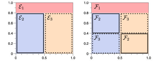
Figure 6: Example D.3.

Example D.3 (Canonical CD, Illustrating Thm. 4.3).

Let $X_{1},X_{2}\sim\textrm{Unif }[0,1]$ and $U$ be an exogenous variable. Let $Y$ be:

$$Y=\begin{cases}X_{1}+U&\text{if }\quad\,\,\,X_{2}\geq 0.8,\\ X_{2}+U&\text{if }\quad\,\,\,X_{1}<0.5\,\,\text{and }X_{2}<0.8,\\ X_{2}+2U&\text{if }\quad\,\,\,X_{1}\geq 0.5\,\,\text{and }X_{2}<0.8.\end{cases}$$

Let ${\mathcal{E}}_{1}=\{(x_{1},x_{2})\mid x_{2}>0.8\}$, ${\mathcal{E}}_{2}=\{(x_{1},x_{2})\mid x_{1}<0.5,x_{2}<0.8\}$, ${\mathcal{E}}_{3}=\{(x_{1},x_{2})\mid x_{1}>0.5,x_{2}<0.8\}$, and ${\mathcal{E}}_{0}=({\mathcal{E}}_{1}\cup{\mathcal{E}}_{2}\cup{\mathcal{E}}_{3})^{c}$. Then, canonical CSSIs $(Y\mathchoice{\mathrel{\hbox to0.0pt{$\displaystyle\perp$\hss}\mkern 3.0mu{\displaystyle\perp}}}{\mathrel{\hbox to0.0pt{$\textstyle\perp$\hss}\mkern 3.0mu{\textstyle\perp}}}{\mathrel{\hbox to0.0pt{$\scriptstyle\perp$\hss}\mkern 3.0mu{\scriptstyle\perp}}}{\mathrel{\hbox to0.0pt{$\scriptscriptstyle\perp$\hss}\mkern 3.0mu{\scriptscriptstyle\perp}}}X_{2}\mid X_{1},{\mathcal{E}}_{1})$, $(Y\mathchoice{\mathrel{\hbox to0.0pt{$\displaystyle\perp$\hss}\mkern 3.0mu{\displaystyle\perp}}}{\mathrel{\hbox to0.0pt{$\textstyle\perp$\hss}\mkern 3.0mu{\textstyle\perp}}}{\mathrel{\hbox to0.0pt{$\scriptstyle\perp$\hss}\mkern 3.0mu{\scriptstyle\perp}}}{\mathrel{\hbox to0.0pt{$\scriptscriptstyle\perp$\hss}\mkern 3.0mu{\scriptscriptstyle\perp}}}X_{1}\mid X_{2},{\mathcal{E}}_{2})$, and $(Y\mathchoice{\mathrel{\hbox to0.0pt{$\displaystyle\perp$\hss}\mkern 3.0mu{\displaystyle\perp}}}{\mathrel{\hbox to0.0pt{$\textstyle\perp$\hss}\mkern 3.0mu{\textstyle\perp}}}{\mathrel{\hbox to0.0pt{$\scriptstyle\perp$\hss}\mkern 3.0mu{\scriptstyle\perp}}}{\mathrel{\hbox to0.0pt{$\scriptscriptstyle\perp$\hss}\mkern 3.0mu{\scriptscriptstyle\perp}}}X_{1}\mid X_{2},{\mathcal{E}}_{3})$ hold. Therefore, $\{({\mathcal{E}}_{0},{\mathbf{X}}),({\mathcal{E}}_{1},{\mathbf{X}}_{1}),({\mathcal{E}}_{2},{\mathbf{X}}_{2}),({\mathcal{E}}_{3},{\mathbf{X}}_{2})\}$ is a canonical CD. On the other hand, let ${\mathcal{F}}_{1}={\mathcal{E}}_{1}$, ${\mathcal{F}}_{2}=\{(x_{1},x_{2})\mid(x_{1}<0.5,0.4<x_{2}<0.8)\text{ or }(x_{1}>0.5,x_{2}<0.4)\}$, ${\mathcal{F}}_{3}=\{(x_{1},x_{2})\mid(x_{1}<0.5,x_{2}<0.4)\text{ or }(x_{1}>0.5,0.4<x_{2}<0.8)\}$, and ${\mathcal{F}}_{0}=({\mathcal{F}}_{1}\cup{\mathcal{F}}_{2}\cup{\mathcal{F}}_{3})^{c}$. Then, canonical CSSIs $(Y\mathchoice{\mathrel{\hbox to0.0pt{$\displaystyle\perp$\hss}\mkern 3.0mu{\displaystyle\perp}}}{\mathrel{\hbox to0.0pt{$\textstyle\perp$\hss}\mkern 3.0mu{\textstyle\perp}}}{\mathrel{\hbox to0.0pt{$\scriptstyle\perp$\hss}\mkern 3.0mu{\scriptstyle\perp}}}{\mathrel{\hbox to0.0pt{$\scriptscriptstyle\perp$\hss}\mkern 3.0mu{\scriptscriptstyle\perp}}}X_{2}\mid X_{1},{\mathcal{F}}_{1})$, $(Y\mathchoice{\mathrel{\hbox to0.0pt{$\displaystyle\perp$\hss}\mkern 3.0mu{\displaystyle\perp}}}{\mathrel{\hbox to0.0pt{$\textstyle\perp$\hss}\mkern 3.0mu{\textstyle\perp}}}{\mathrel{\hbox to0.0pt{$\scriptstyle\perp$\hss}\mkern 3.0mu{\scriptstyle\perp}}}{\mathrel{\hbox to0.0pt{$\scriptscriptstyle\perp$\hss}\mkern 3.0mu{\scriptscriptstyle\perp}}}X_{1}\mid X_{2},{\mathcal{F}}_{2})$, and $(Y\mathchoice{\mathrel{\hbox to0.0pt{$\displaystyle\perp$\hss}\mkern 3.0mu{\displaystyle\perp}}}{\mathrel{\hbox to0.0pt{$\textstyle\perp$\hss}\mkern 3.0mu{\textstyle\perp}}}{\mathrel{\hbox to0.0pt{$\scriptstyle\perp$\hss}\mkern 3.0mu{\scriptstyle\perp}}}{\mathrel{\hbox to0.0pt{$\scriptscriptstyle\perp$\hss}\mkern 3.0mu{\scriptscriptstyle\perp}}}X_{1}\mid X_{2},{\mathcal{F}}_{3})$ hold. Therefore, $\{({\mathcal{F}}_{0},{\mathbf{X}}),({\mathcal{F}}_{1},{\mathbf{X}}_{1}),({\mathcal{F}}_{2},{\mathbf{X}}_{2}),({\mathcal{F}}_{3},{\mathbf{X}}_{2})\}$ is a canonical CD. Here, $p({\mathcal{E}}_{2}\cap{\mathcal{F}}_{2})>0$ and thus $\mathbf{pa}^{{\mathcal{E}}_{2}}=\mathbf{pa}^{{\mathcal{F}}_{2}}={\mathbf{X}}_{2}$ by Thm. 4.3. Also, ${\mathcal{E}}[{\mathbf{X}}_{2}]={\mathcal{E}}_{2}\cup{\mathcal{E}}_{3}={\mathcal{F}}_{2}\cup{\mathcal{F}}_{3}={\mathcal{F}}[{\mathbf{X}}_{2}]$ by Thm. 4.3.

Appendix E Experimental Details

E.1 Synthetic datasets

We provide the details of the configurations of the causal system in our experiments. The following causal system is the case of uniformly distributed local parent sets with a linear boundary. Here, $g$ is a linear function implemented with a randomly initialized NN.

$$Y=\begin{cases}f_{1}({\mathbf{X}}_{123},N)&\text{if }\quad\,\,\,g(\mathbf{x}_{147})=\max(g(\mathbf{x}_{147}),g(\mathbf{x}_{258}),g(\mathbf{x}_{369})),\\ f_{2}({\mathbf{X}}_{456},N)&\text{if }\quad\,\,\,g(\mathbf{x}_{258})=\max(g(\mathbf{x}_{147}),g(\mathbf{x}_{258}),g(\mathbf{x}_{369})),\\ f_{3}({\mathbf{X}}_{789},N)&\text{if }\quad\,\,\,g(\mathbf{x}_{369})=\max(g(\mathbf{x}_{147}),g(\mathbf{x}_{258}),g(\mathbf{x}_{369})).\end{cases}$$ (10)

The following is the case of uniformly distributed local parent sets with a nonlinear boundary determined by the norm:

$$Y=\begin{cases}f_{1}({\mathbf{X}}_{123},N)&\text{if }\quad\,\,\,\|\mathbf{x}\|<c_{1},\\ f_{2}({\mathbf{X}}_{456},N)&\text{if }\quad\,\,\,c_{1}<\|\mathbf{x}\|<c_{2},\\ f_{3}({\mathbf{X}}_{789},N)&\text{if }\quad\,\,\,\|\mathbf{x}\|>c_{2}.\end{cases}$$ (11)

The following is the case of uniformly distributed local parent sets with a nonlinear boundary determined by a linear function $g$ implemented with a NN:

$$Y=\begin{cases}f_{1}({\mathbf{X}}_{123},N)&\text{if }\quad\,\,\,g(\mathbf{x}_{147})=\max(g(\mathbf{x}_{147}),g(\mathbf{x}_{258}),g(\mathbf{x}_{369})),\\ f_{2}({\mathbf{X}}_{456},N)&\text{if }\quad\,\,\,g(\mathbf{x}_{258})=\max(g(\mathbf{x}_{147}),g(\mathbf{x}_{258}),g(\mathbf{x}_{369})),\\ f_{3}({\mathbf{X}}_{789},N)&\text{if }\quad\,\,\,g(\mathbf{x}_{369})=\max(g(\mathbf{x}_{147}),g(\mathbf{x}_{258}),g(\mathbf{x}_{369})).\end{cases}$$ (12)

The following causal system is the case of non-uniformly distributed local parent sets with a linear boundary. Here, $g$ is a linear function implemented with a randomly initialized NN.

$$Y=\begin{cases}f_{1}({\mathbf{X}}_{123},N)&\text{if }\quad\,\,\,g(\mathbf{x}_{147})=\max(g(\mathbf{x}_{147}),g(\mathbf{x}_{258}),g(\mathbf{x}_{369})),\\ f_{2}({\mathbf{X}}_{456789},N)&\text{if }\quad\,\,\,g(\mathbf{x}_{258})=\max(g(\mathbf{x}_{147}),g(\mathbf{x}_{258}),g(\mathbf{x}_{369})),\\ f_{3}({\mathbf{X}},N)&\text{if }\quad\,\,\,g(\mathbf{x}_{369})=\max(g(\mathbf{x}_{147}),g(\mathbf{x}_{258}),g(\mathbf{x}_{369})).\end{cases}$$ (13)

The following is the case of non-uniformly distributed local parent sets with a nonlinear boundary determined by the norm:

$$Y=\begin{cases}f_{1}({\mathbf{X}}_{123},N)&\text{if }\quad\,\,\,\|\mathbf{x}\|<c_{1},\\ f_{2}({\mathbf{X}}_{456789},N)&\text{if }\quad\,\,\,c_{1}<\|\mathbf{x}\|<c_{2},\\ f_{3}({\mathbf{X}},N)&\text{if }\quad\,\,\,\|\mathbf{x}\|>c_{2}.\end{cases}$$ (14)

The following is the case of non-uniformly distributed local parent sets with a nonlinear boundary determined by a nonlinear function $g$ implemented with a NN:

$$Y=\begin{cases}f_{1}({\mathbf{X}}_{123},N)&\text{if }\quad\,\,\,g(\mathbf{x}_{147})=\max(g(\mathbf{x}_{147}),g(\mathbf{x}_{258}),g(\mathbf{x}_{369})),\\ f_{2}({\mathbf{X}}_{456789},N)&\text{if }\quad\,\,\,g(\mathbf{x}_{258})=\max(g(\mathbf{x}_{147}),g(\mathbf{x}_{258}),g(\mathbf{x}_{369})),\\ f_{3}({\mathbf{X}},N)&\text{if }\quad\,\,\,g(\mathbf{x}_{369})=\max(g(\mathbf{x}_{147}),g(\mathbf{x}_{258}),g(\mathbf{x}_{369})).\end{cases}$$ (15)

For the toy experiment for the visualization of the decision boundary, we let $X_{1},X_{2}\sim\mathcal{N}(0,I_{3})$ and $Y=f_{1}(X_{1})$ if $\|(X_{1},X_{2})\|<\epsilon$ and $f_{2}(X_{2})$ otherwise. For the linear function $g$, we used a randomly initialized linear layer. For the nonlinear function $g$, we used a randomly initialized NN with a single hidden layer, 10 hidden units, and Tanh activation. The total number of data samples is 50000, with a ratio of 8:1:1 of training, validation, and held-out test set, respectively.

Figure 7: Example images of the Spriteworld environment.

E.2 Spriteworld

While the original environment does not consider the interaction between objects, Pitis et al. (2020) modified the environment to devise the collision between moving objects and to acquire the ground truth local causal graphs. Our experiment was also conducted in the modified Spriteworld, which we denote as Spriteworld for simplicity. In this environment, there are moving objects in the scene. Following real-world dynamics, objects can collide with each other, and thus each object has an influence on others. However, their position and velocity will be affected by the others only when they collide, which occurs relatively rarely. In other words, the state of each object will only be determined by its own state in the previous time-step in most cases. Example images of the Spriteworld environment are shown in Fig. 7. In the setting of Pitis et al. (2020), each variables represent corresponding objects, i.e., $X_{i}=(x,y,v_{x},v_{y})_{i}$ represents the $i$-th object. Thus, ${\mathbf{X}}=\{X_{1},\cdots,X_{n+1}\}$ and ${\mathbf{Y}}=\{Y_{1},\cdots,Y_{n}\}$. In our experiment, we consider a more complex setup where each variable represents the position and velocity of each object, thus ${\mathbf{X}}=\{X_{1},\cdots,X_{2n+1}\}$ and ${\mathbf{Y}}=\{Y_{1},\cdots,Y_{2n}\}$. Further, we also include the exogenous variable.

E.3 Implementation.

Implementation details.

For the implementation of our model, the distribution $p_{\theta}(y|x,z)$ could be any distribution as long as the log-likelihood is computable, and we chose Gaussian for simplicity. We note that ground truth $p(y|x,z)$ is non-Gaussian (i.e., non-linear function with non-additive noise model) in our experiments. For $f_{\theta}(\mathbf{x},z)$, which approximates the conditional distribution $P(Y\mid\mathbf{X},Z)$, and $g_{\phi}(\mathbf{x})$, which outputs the parameters of Bernoulli distribution, we used an MLP with 3 hidden layers and 128 hidden units. For all the experiments, we set the batch size to 1000 and used the Adam optimizer with the weight decay of $10^{-5}$. We set the learning rate of $10^{-2}$ for the synthetic dataset and $10^{-3}$ for the Spriteworld. Most experiments were conducted with a single RTX 3090 GPU. For the mixture model and the transformer model, we used 3 MLPs, each with 3 hidden layers and 128 hidden units, and grid-search the learning rate over $\{0.005,0.01,0.02,0.03\}$.

Regularizer.

One can adopt a regularizer to induce a sparse solution and prevent the model from outputting a trivial solution $z=(1,1,\cdots,1)$ where $z\sim g_{\phi}(\mathbf{x})$, e.g., adding a term $\lambda\cdot\|g_{\phi}(\mathbf{x})\|_{1}$. During our experiments, however, we empirically found that the regularizer does not significantly bring a gain. We hypothesized that since the neural network $\phi$ is randomly initialized, approximately half of the entries of $z$ would be $0$ at the beginning of the training, and, consequently, it would rarely converge to the trivial solution $z=(1,1,\cdots,1)$.

Gumbel-Softmax.

Although there are other methods used for learning discrete variables, such as a REINFORCE estimator, we chose Gumbel-Softmax (Jang et al., 2016; Maddison et al., 2016) since it (i) has a lower variance compared to REINFORCE estimator, and (ii) is empirically shown to be more effective (Jang et al., 2016; Maddison et al., 2016; Ng et al., 2019). Given that the choice of reparametrization trick is not the main focus of our work, we did not compare it to other estimators.

Evaluation.

We now describe the procedure for plotting the ROC curve. Let $Pa(Y)=\{1,2,\cdots,9\}$ (i.e., $d=9$). Consider a single data point $\mathbf{x}$ where $A_{true}=\{1\}$, and the model predicted $A_{pred}=\{1,2\}$ with a threshold $\tau$. In this case, $TP=1$, $FP=1$, $FN=0$, and $TN=7$. We note that this evaluation procedure follows the prior work (Pitis et al., 2020). We plot the ROC curves based on all the data points in a test dataset. Accordingly, $TP+FP+FN+TN=B\times d$ where $B$ is the number of test data points. Each data point belongs to one of the partitioned sets (i.e., region), and the number of data points for each region is similar. Train and test distributions are identical.

Appendix F Additional Experiments

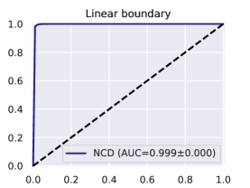
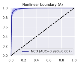
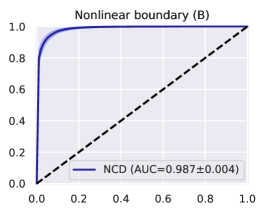
Figure 8: ROC curves for the ground truth local independence relationships on the synthetic dataset of the additive noise model.

Here, we provide the experimental results on the synthetic datasets where the functions are nonlinear with an additive noise model. We consider the following causal system with a linear boundary determined by a linear function $g$:

$$Y=\begin{cases}f_{1}({\mathbf{X}}_{123})+N&\text{if }\quad\,\,\,g(\mathbf{x}_{147})=\max(g(\mathbf{x}_{147}),g(\mathbf{x}_{258}),g(\mathbf{x}_{369})),\\ f_{2}({\mathbf{X}}_{456})+N&\text{if }\quad\,\,\,g(\mathbf{x}_{258})=\max(g(\mathbf{x}_{147}),g(\mathbf{x}_{258}),g(\mathbf{x}_{369})),\\ f_{3}({\mathbf{X}}_{789})+N&\text{if }\quad\,\,\,g(\mathbf{x}_{369})=\max(g(\mathbf{x}_{147}),g(\mathbf{x}_{258}),g(\mathbf{x}_{369})).\end{cases}$$ (16)

The following is the case of a nonlinear boundary determined by the norm:

$$Y=\begin{cases}f_{1}({\mathbf{X}}_{123})+N&\text{if }\quad\,\,\,\|\mathbf{x}\|<c_{1},\\ f_{2}({\mathbf{X}}_{456})+N&\text{if }\quad\,\,\,c_{1}<\|\mathbf{x}\|<c_{2},\\ f_{3}({\mathbf{X}}_{789})+N&\text{if }\quad\,\,\,\|\mathbf{x}\|>c_{2}.\end{cases}$$ (17)

The following is the case of a nonlinear boundary determined by a nonlinear function $g$:

$$Y=\begin{cases}f_{1}({\mathbf{X}}_{123})+N&\text{if }\quad\,\,\,g(\mathbf{x}_{147})=\max(g(\mathbf{x}_{147}),g(\mathbf{x}_{258}),g(\mathbf{x}_{369})),\\ f_{2}({\mathbf{X}}_{456})+N&\text{if }\quad\,\,\,g(\mathbf{x}_{258})=\max(g(\mathbf{x}_{147}),g(\mathbf{x}_{258}),g(\mathbf{x}_{369})),\\ f_{3}({\mathbf{X}}_{789})+N&\text{if }\quad\,\,\,g(\mathbf{x}_{369})=\max(g(\mathbf{x}_{147}),g(\mathbf{x}_{258}),g(\mathbf{x}_{369})).\end{cases}$$ (18)

As shown in Fig. 8, our method successfully discovers the local independence relationships in the additive noise system as well.

References

- Angrist and Pischke (2008) Joshua D Angrist and Jörn-Steffen Pischke. Mostly harmless econometrics. Princeton university press, 2008.
- Angrist et al. (1996) Joshua D Angrist, Guido W Imbens, and Donald B Rubin. Identification of causal effects using instrumental variables. Journal of the American statistical Association, 91(434):444–455, 1996.
- Banerjee et al. (2016) Abhijit Vinayak Banerjee, Esther Duflo, and Michael Kremer. The influence of randomized controlled trials on development economics research and on development policy. The State of Economics, The State of the World, pages 482–488, 2016.
- Boutilier et al. (2013) Craig Boutilier, Nir Friedman, Moisés Goldszmidt, and Daphne Koller. Context-specific independence in bayesian networks. CoRR, abs/1302.3562, 2013.
- Brouillard et al. (2020) Philippe Brouillard, Sébastien Lachapelle, Alexandre Lacoste, Simon Lacoste-Julien, and Alexandre Drouin. Differentiable causal discovery from interventional data. arXiv preprint arXiv:2007.01754, 2020.
- Chicharro et al. (2020) Daniel Chicharro, Michel Besserve, and Stefano Panzeri. Causal learning with sufficient statistics: an information bottleneck approach. arXiv preprint arXiv:2010.05375, 2020.
- Chickering (2002) David Maxwell Chickering. Optimal structure identification with greedy search. Journal of machine learning research, 3(Nov):507–554, 2002.
- Dal et al. (2018) Giso H Dal, Alfons W Laarman, and Peter JF Lucas. Parallel probabilistic inference by weighted model counting. In International Conference on Probabilistic Graphical Models, pages 97–108. PMLR, 2018.
- Glymour et al. (2019) Clark Glymour, Kun Zhang, and Peter Spirtes. Review of causal discovery methods based on graphical models. Frontiers in genetics, 10:524, 2019.
- Gogate and Domingos (2010) Vibhav Gogate and Pedro Domingos. Exploiting logical structure in lifted probabilistic inference. In Workshops at the Twenty-Fourth AAAI Conference on Artificial Intelligence, 2010.
- Hoyer et al. (2008) Patrik O Hoyer, Dominik Janzing, Joris Mooij, Jonas Peters, and Bernhard Schölkopf. Nonlinear causal discovery with additive noise models. In Proceedings of the 21st International Conference on Neural Information Processing Systems, pages 689–696, 2008.
- Imbens (2020) Guido W Imbens. Potential outcome and directed acyclic graph approaches to causality: Relevance for empirical practice in economics. Journal of Economic Literature, 58(4):1129–79, 2020.
- Imbens and Rubin (2015) Guido W Imbens and Donald B Rubin. Causal inference in statistics, social, and biomedical sciences. Cambridge University Press, 2015.
- Jang et al. (2016) Eric Jang, Shixiang Gu, and Ben Poole. Categorical reparameterization with gumbel-softmax. arXiv preprint arXiv:1611.01144, 2016.
- Kalainathan et al. (2022) Diviyan Kalainathan, Olivier Goudet, Isabelle Guyon, David Lopez-Paz, and Michèle Sebag. Structural agnostic modeling: Adversarial learning of causal graphs. Journal of Machine Learning Research, 23(219):1–62, 2022.
- Lachapelle et al. (2020) Sébastien Lachapelle, Philippe Brouillard, Tristan Deleu, and Simon Lacoste-Julien. Gradient-based neural dag learning. In International Conference on Learning Representations, 2020.
- Maddison et al. (2016) Chris J Maddison, Andriy Mnih, and Yee Whye Teh. The concrete distribution: A continuous relaxation of discrete random variables. arXiv preprint arXiv:1611.00712, 2016.
- Ng et al. (2019) Ignavier Ng, Zhuangyan Fang, Shengyu Zhu, Zhitang Chen, and Jun Wang. Masked gradient-based causal structure learning. arXiv preprint arXiv:1910.08527, 2019.
- Nyman et al. (2017) Henrik Nyman, Johan Pensar, and Jukka Corander. Stratified gaussian graphical models. Communications in Statistics-Theory and Methods, 46(11):5556–5578, 2017.
- Pearl (2009) Judea Pearl. Causality. Cambridge university press, 2009.
- Pensar et al. (2015) Johan Pensar, Henrik Nyman, Timo Koski, and Jukka Corander. Labeled directed acyclic graphs: a generalization of context-specific independence in directed graphical models. Data mining and knowledge discovery, 29(2):503–533, 2015.
- Pensar et al. (2016) Johan Pensar, Henrik Nyman, Jarno Lintusaari, and Jukka Corander. The role of local partial independence in learning of bayesian networks. International journal of approximate reasoning, 69:91–105, 2016.
- Peters (2015) Jonas Peters. On the intersection property of conditional independence and its application to causal discovery. Journal of Causal Inference, 3(1):97–108, 2015.
- Peters et al. (2017) Jonas Peters, Dominik Janzing, and Bernhard Schölkopf. Elements of causal inference: foundations and learning algorithms. The MIT Press, 2017.
- Pitis et al. (2020) Silviu Pitis, Elliot Creager, and Animesh Garg. Counterfactual data augmentation using locally factored dynamics. Advances in Neural Information Processing Systems, 33, 2020.
- Poole (1998) David Poole. Context-specific approximation in probabilistic inference. In Proceedings of the Fourteenth conference on Uncertainty in artificial intelligence, pages 447–454, 1998.
- Poole and Zhang (2003) David Poole and Nevin Lianwen Zhang. Exploiting contextual independence in probabilistic inference. Journal of Artificial Intelligence Research, 18:263–313, 2003.
- Robins et al. (2020) James M Robins, Thomas S Richardson, and Ilya Shpitser. An interventionist approach to mediation analysis. arXiv preprint arXiv:2008.06019, 2020.
- Seitzer et al. (2021) Maximilian Seitzer, Bernhard Schölkopf, and Georg Martius. Causal influence detection for improving efficiency in reinforcement learning. Advances in Neural Information Processing Systems, 34:22905–22918, 2021.
- Shimizu et al. (2006) Shohei Shimizu, Patrik O Hoyer, Aapo Hyvärinen, Antti Kerminen, and Michael Jordan. A linear non-gaussian acyclic model for causal discovery. Journal of Machine Learning Research, 7(10), 2006.
- Shipley (2016) Bill Shipley. Cause and correlation in biology: a user’s guide to path analysis, structural equations and causal inference with R. Cambridge University Press, 2016.
- Sobel (1995) Michael E Sobel. Causal inference in the social and behavioral sciences. In Handbook of statistical modeling for the social and behavioral sciences, pages 1–38. Springer, 1995.
- Spirtes et al. (2000) Pater Spirtes, Clark Glymour, Richard Scheines, Stuart Kauffman, Valerio Aimale, and Frank Wimberly. Constructing Bayesian network models of gene expression networks from microarray data. 2000.
- Tikka et al. (2019) Santtu Tikka, Antti Hyttinen, and Juha Karvanen. Identifying causal effects via context-specific independence relations. Advances in Neural Information Processing Systems, 32:2804–2814, 2019.
- Van den Broeck et al. (2011) Guy Van den Broeck, Nima Taghipour, Wannes Meert, Jesse Davis, and Luc De Raedt. Lifted probabilistic inference by first-order knowledge compilation. In Proceedings of the Twenty-Second international joint conference on Artificial Intelligence, pages 2178–2185, 2011.
- Vaswani et al. (2017) Ashish Vaswani, Noam Shazeer, Niki Parmar, Jakob Uszkoreit, Llion Jones, Aidan N Gomez, Łukasz Kaiser, and Illia Polosukhin. Attention is all you need. In Advances in neural information processing systems, pages 5998–6008, 2017.
- Wang et al. (2017) Yuhao Wang, Liam Solus, Karren Dai Yang, and Caroline Uhler. Permutation-based causal inference algorithms with interventions. In Proceedings of the 31st International Conference on Neural Information Processing Systems, pages 5824–5833, 2017.
- Watters et al. (2019) Nicholas Watters, Loic Matthey, Matko Bosnjak, Christopher P Burgess, and Alexander Lerchner. Cobra: Data-efficient model-based rl through unsupervised object discovery and curiosity-driven exploration. arXiv preprint arXiv:1905.09275, 2019.
- Yu et al. (2019) Yue Yu, Jie Chen, Tian Gao, and Mo Yu. Dag-gnn: Dag structure learning with graph neural networks. In International Conference on Machine Learning, pages 7154–7163. PMLR, 2019.
- Zhang et al. (2011) Kun Zhang, Jonas Peters, Dominik Janzing, and Bernhard Schölkopf. Kernel-based conditional independence test and application in causal discovery. In 27th Conference on Uncertainty in Artificial Intelligence (UAI 2011), pages 804–813. AUAI Press, 2011.
- Zheng et al. (2018) Xun Zheng, Bryon Aragam, Pradeep K Ravikumar, and Eric P Xing. DAGs with NO TEARS: Continuous optimization for structure learning. Advances in Neural Information Processing Systems, 31, 2018.
- Zhu et al. (2019) Shengyu Zhu, Ignavier Ng, and Zhitang Chen. Causal discovery with reinforcement learning. In International Conference on Learning Representations, 2019.