A complete pair of solvents
of a quadratic matrix pencil

Abstract.

Let $B$ and $C$ be square complex matrices. The differential equation

$$x^{\prime\prime}(t)+Bx^{\prime}(t)+Cx(t)=f(t)$$

is considered. A solvent is a matrix solution $X$ of the equation $X^{2}+BX+C=\mathbf{0}$. A pair of solvents $X$ and $Z$ is called complete if the matrix $X-Z$ is invertible. Knowing a complete pair of solvents $X$ and $Z$ allows us to reduce the solution of the initial value problem to the calculation of two matrix exponentials $e^{Xt}$ and $e^{Zt}$. The problem of finding a complete pair $X$ and $Z$, which leads to small rounding errors in solving the differential equation, is discussed.

Introduction

The characteristic function of the second order linear differential equation

$$x^{\prime\prime}(t)+Bx^{\prime}(t)+Cx(t)=f(t)$$

with constant matrix coefficients $B$ and $C$ is the matrix pencil

$$L(\lambda)=\lambda^{2}\mathbf{1}+\lambda B+C,\qquad\lambda\in\mathbb{C}.$$

A matrix solution of the equation

$$X^{2}+BX+C=\mathbf{0}$$

is called [15, § 3] a (right) solvent of the pencil. They say [4, p. 75] (cf. [15, p. 392]) that two right solvents $X$ and $Z$ form a complete pair if the matrix $X-Z$ is invertible. If one has a complete pair of right solvents, the solution of the differential equation with the initial conditions

$$x(0) =u_{0},$$

$$x^{\prime}(0) =u_{1}$$

can be represented (see Theorem 2 Corollary 11 for more details) in the form

$$x(t)=U^{\prime}(t)u_{0}+U(t)(u_{1}+Bu_{0})+\int_{0}^{t}U(t-s)f(s)\,ds,$$

where

$$U(t) =\bigl{(}e^{Xt}-e^{Zt}\bigr{)}(X-Z)^{-1},$$

$$U^{\prime}(t) =\bigl{(}Xe^{Xt}-Ze^{Zt}\bigr{)}(X-Z)^{-1}.$$

These formulas show that if a complete pair of right solvents is known, then solving the initial value problem is essentially reduced to the calculation of two matrix exponentials $e^{Xt}$ and $e^{Zt}$. This idea was first appeared in [12] and later was discussed by many authors, see, e. g., [13, 15, 16, 20, 21, 22, 26, 27, 30, 31, 32, 33].

We consider matrices $B$ and $C$ of small size (about $10\times 10$ or slightly larger). Only in this case, the representation of matrix exponentials as a function depending on $t$ is not very cumbersome and hence can be effectively used. On the other hand, in the same case the whole set of pairs of right solvents $X$ and $Z$ can be calculated; we describe a corresponding algorithm in Section 3. The aim of the paper is to call attention to the fact that different pairs of right solvents $X$ and $Z$ are not interchangeable. The reason is that when constructing $U(t)$ we perform some linear algebra operations that may or may not be badly conditioned; for example, the condition number $\varkappa(X-Z)=\lVert X-Z\rVert\cdot\lVert(X-Z)^{-1}\rVert$ may be large, which leads to large errors when multiplying by $(X-Z)^{-1}$.

There are many papers devoted to numerical calculation of solvents, see, e. g., [1, 7, 8, 10, 11, 34, 35]. The present paper is distinguished by the formulation of the problem: we look for a complete pair of solvents that leads to small rounding errors.

The paper is organized as follows. In Sections 1, we recall general information connected with quadratic pencils and their right solvents. In Section 2, we recall some facts related to Jordan chains of a quadratic pencil and its companion matrix. In Section 3, we describe a spectral algorithm of finding a right solvent. In Sections 4, we describe how to find all complete pairs of right solvents and to choose the best one. In Section 5, we present a few numerical examples.

1. Quadratic pencils and right solvents

In this section, we collect some general definitions and recall some general facts.

Let $n\in\mathbb{N}$. We denote by $\mathbb{C}^{n\times n}$ the linear space of all complex matrices of the size $n\times n$; the symbol $\mathbf{1}\in\mathbb{C}^{n\times n}$ denotes the identical matrix, and the symbol $\mathbf{0}\in\mathbb{C}^{n\times n}$ denotes the zero matrix. Usually we do not distinguish matrices and the operators in $\mathbb{C}^{n}$ induced by them.

Definition 1.

Let $n\in\mathbb{N}$ and $B,C\in\mathbb{C}^{n\times n}$. We consider the second order linear differential equation

$$x^{\prime\prime}(t)+Bx^{\prime}(t)+Cx(t)=f(t).$$ (1)

The (quadratic) pencil corresponding to (1) is the function

$$L(\lambda)=\lambda^{2}\mathbf{1}+\lambda B+C,\qquad\lambda\in\mathbb{C},$$ (2)

with values in $\mathbb{C}^{n\times n}$. The resolvent of pencil (2) is the function

$$R_{\lambda}=(\lambda^{2}\mathbf{1}+\lambda B+C)^{-1},$$

and the resolvent set of pencil (2) is the set $\rho(B,C)$, consisting of all $\lambda\in\mathbb{C}$ such that this inverse exists. The spectrum of the pencil is the complement $\sigma(B,C)=\mathbb{C}\setminus\rho(B,C)$ of the resolvent set.

Similarly, $\rho(X)$ and $\sigma(X)$ respectively denote the resolvent set and the spectrum of a matrix $X\in\mathbb{C}^{n\times n}$.

Let $U$ be an open set that contains $\sigma(B,C)$ and $f:\,U\to\mathbb{C}$ be a holomorphic function. We consider the matrices

$$\psi(f) =\frac{1}{2\pi i}\int_{\Gamma}f(\lambda)(\lambda^{2}\mathbf{1}+\lambda B+C)^{-1}\,d\lambda,$$ (3)

$$\chi(f) =\frac{1}{2\pi i}\int_{\Gamma}\lambda f(\lambda)(\lambda^{2}\mathbf{1}+\lambda B+C)^{-1}\,d\lambda,$$ (4)

where $\Gamma$ is a contour laying in $U$, oriented counterclockwise, and surrounding $\sigma(B,C)$.

We set $U(t)=\psi(\exp_{t})$, where $\exp_{t}(\lambda)=e^{\lambda t}$, or more detailed

$$U(t)=\frac{1}{2\pi i}\int_{\Gamma}e^{\lambda t}(\lambda^{2}\mathbf{1}+\lambda B+C)^{-1}\,d\lambda.$$ (5)

Obviously, differentiating (5) with respect to $t$, we obtain

$$U^{\prime}(t)=\frac{1}{2\pi i}\int_{\Gamma}\lambda e^{\lambda t}(\lambda^{2}\mathbf{1}+\lambda B+C)^{-1}\,d\lambda=\chi(\exp_{t}).$$ (6)

Proposition 1.

The following identities hold:

$$U(0)=\mathbf{0},\qquad U^{\prime}(0)=\mathbf{1}.$$

Proof.

We have (the symbol $\operatorname{Res}$ means residue)

$$\lim_{\lambda\to\infty}R_{\lambda} =\lim_{\lambda\to\infty}\frac{1}{\lambda^{2}}\Bigl{(}\mathbf{1}+\frac{1}{\lambda}B+\frac{1}{\lambda^{2}}C\Bigr{)}^{-1}=\mathbf{0},$$

$$\lim_{\lambda\to\infty}\lambda R_{\lambda} =\lim_{\lambda\to\infty}\frac{1}{\lambda}\Bigl{(}\mathbf{1}+\frac{1}{\lambda}B+\frac{1}{\lambda^{2}}C\Bigr{)}^{-1}=\mathbf{0},$$

$$U(0) =\frac{1}{2\pi i}\int_{\Gamma}(\lambda^{2}\mathbf{1}+\lambda B+C)^{-1}\,d\lambda$$

$$=\operatorname{Res}_{\lambda=\infty}(\lambda^{2}\mathbf{1}+\lambda B+C)^{-1}$$

$$=\lim_{\lambda\to\infty}\lambda(\lambda^{2}\mathbf{1}+\lambda B+C)^{-1}$$

$$=\lim_{\lambda\to\infty}\frac{1}{\lambda}\Bigl{(}\mathbf{1}+\frac{1}{\lambda}B+\frac{1}{\lambda^{2}}C\Bigr{)}^{-1}=\mathbf{0},$$

$$U^{\prime}(0) =\frac{1}{2\pi i}\int_{\Gamma}\lambda(\lambda^{2}\mathbf{1}+\lambda B+C)^{-1}\,d\lambda$$

$$=\operatorname{Res}_{\lambda=\infty}\lambda(\lambda^{2}\mathbf{1}+\lambda B+C)^{-1}$$

$$=\lim_{\lambda\to\infty}\lambda^{2}(\lambda^{2}\mathbf{1}+\lambda B+C)^{-1}$$

$$=\lim_{\lambda\to\infty}\Bigl{(}\mathbf{1}+\frac{1}{\lambda}B+\frac{1}{\lambda^{2}}C\Bigr{)}^{-1}=\mathbf{1}.\qed$$

Theorem 2 (see, e.g., [17, Theorem 16]).

Let $f:\,\mathbb{R}\to\mathbb{C}^{n}$ be a continuous function. Then the solution $x$ of the initial value problem

$$\begin{split}x^{\prime\prime}(t)+Bx^{\prime}(t)+Cx(t)&=f(t),\qquad t\in\mathbb{R},\\ x(0)&=u_{0},\\ x^{\prime}(0)&=u_{1}\end{split}$$ (7)

and its derivative can be represented in the form

$$x(t) =U^{\prime}(t)u_{0}+U(t)(u_{1}+Bu_{0})+\int_{0}^{t}U(t-s)f(s)\,ds, t\in\mathbb{R},$$ (8)

$$x^{\prime}(t) =U^{\prime}(t)u_{1}-U(t)Cu_{0}+\int_{0}^{t}U^{\prime}(t-s)f(s)\,ds, t\in\mathbb{R}.$$

Definition 2.

A matrix $X\in\mathbb{C}^{n\times n}$ is called [15, § 3] a (right) solvent of pencil (2) if $X$ satisfies the equation

$$X^{2}+BX+C=\mathbf{0}.$$

A left solvent is defined as a solution of the equation

$$Y^{2}+YB+C=\mathbf{0}.$$

In this paper we deal only with right solvents.

Not every quadratic pencil has at least one solvent, see Example 2 below.

Definition 3.

A factorization of pencil (2) is its representation as the product of two linear pencils:

$$\lambda^{2}\mathbf{1}+\lambda B+C=(\lambda\mathbf{1}-Y)(\lambda\mathbf{1}-X),$$ (9)

where $X,Y\in\mathbb{C}^{n\times n}$.

Proposition 3.

Let pencil (2) possess factorization (9). Then

$$\sigma(B,C)=\sigma(X)\cup\sigma(Y).$$

Proof.

Let $\lambda\in\sigma(X)$. Then the kernel of the matrix $\lambda\mathbf{1}-X$ is non-zero. From formula (9) it is seen that the kernel of the matrix $\lambda^{2}\mathbf{1}+\lambda B+C$ is also non-zero.

Now let $\lambda\in\sigma(Y)$. Then the image of the matrix $\lambda\mathbf{1}-Y$ does not coincide with the whole $\mathbb{C}^{n}$. Then from (9) it is seen that the image of the matrix $\lambda^{2}\mathbf{1}+\lambda B+C$ also does not coincides with $\mathbb{C}^{n}$.

Finally, let $\lambda\in\sigma(B,C)$. Then the matrix $\lambda^{2}\mathbf{1}+\lambda B+C$ has a non-zero kernel. Let, for definiteness, a non-zero vector $h$ belong to $\operatorname{Ker}(\lambda^{2}\mathbf{1}+\lambda B+C)$. Then from (9) it is seen that $(\lambda\mathbf{1}-Y)(\lambda\mathbf{1}-X)h=0$. Consequently, we have either $(\lambda\mathbf{1}-X)h=0$ or $(\lambda\mathbf{1}-Y)u=0$, where $u=(\lambda\mathbf{1}-X)h$ with $u\neq 0$. In other words, either $\lambda\mathbf{1}-Y$ or $\lambda\mathbf{1}-X$ has a non-zero kernel. ∎

Theorem 4 ([3, p. 81], [15, p. 389]).

Let $X$ be a right solvent of the equation

$$X^{2}+BX+C=\mathbf{0}.$$

Then

$$\lambda^{2}\mathbf{1}+\lambda B+C=(\lambda\mathbf{1}+X+B)(\lambda\mathbf{1}-X).$$

Definition 4.

A pair of right solvents $X$ and $Z$ is called [4, p. 75] (cf. [15, p. 392]) complete if the matrix $X-Z$ is invertible.

Even if a pencil has a right solvent, there is not always another right solvent $Z$ such that the pair $X$ and $Z$ is complete, see Example 3 below.

Theorem 10 below and its Corollary 11 show that as soon as two right solvents form a complete pair, the calculation of matrices (3) and (4) is reduced to the calculation of two functions of linear pencils, which significantly simplifies the calculation of the matrices (3) and (4) or (5) and (6). This explains the importance of the problem of finding a complete pair.

Lemma 5.

Let $X$ and $Z$ be arbitrary right solvents of pencil (2). Then

$$(X^{2}-Z^{2})+B(X-Z)=0.$$ (10)

Proof.

Subtracting $Z^{2}+BZ+C=\mathbf{0}$ from $X^{2}+BX+C=\mathbf{0}$, we arrive at (10). ∎

Proposition 6 ([15, p. 393, Lemma 4.1]).

Let $X$ and $Z$ be arbitrary right solvents of pencil (2). Then for any $\lambda\in\rho(B,C)\cap\rho(X)\cap\rho(Z)$ the following identities hold:

$$(\lambda^{2}\mathbf{1}+\lambda B+C)^{-1}(X-Z) =(\lambda\mathbf{1}-X)^{-1}(X-Z)(\lambda\mathbf{1}-Z)^{-1}$$

$$=(\lambda\mathbf{1}-Z)^{-1}(X-Z)(\lambda\mathbf{1}-X)^{-1}$$

$$=(\lambda\mathbf{1}-X)^{-1}-(\lambda\mathbf{1}-Z)^{-1}.$$

Proof.

By Theorem 4, for $\lambda\in\rho(X)$ we have

$$(\lambda^{2}\mathbf{1}+\lambda B+C)(\lambda\mathbf{1}-X)^{-1}=\lambda\mathbf{1}+X+B.$$

Hence, taking into account equality (10), we obtain that

$$(\lambda^{2}\mathbf{1} +\lambda B+C)(\lambda\mathbf{1}-X)^{-1}(X-Z)=(\lambda\mathbf{1}+X+B)(X-Z)$$

$$=\lambda(X-Z)+X(X-Z)+B(X-Z)$$

$$=\lambda(X-Z)+X(X-Z)+Z^{2}-X^{2}$$

$$=\lambda(X-Z)+Z^{2}-XZ$$

$$=\lambda(X-Z)-(X-Z)Z$$

$$=(X-Z)(\lambda\mathbf{1}-Z).$$

Multiplying the resulting equality by $(\lambda^{2}\mathbf{1}+\lambda B+C)^{-1}$ on the left and by $(\lambda\mathbf{1}-Z)^{-1}$ on the right, we obtain the first formula. The second formula follows from the first one by symmetry.

To prove the last formula, we note that

$$(\lambda\mathbf{1}-Z)^{-1}(X-Z)(\lambda\mathbf{1}-X)^{-1}\\ =(\lambda\mathbf{1}-Z)^{-1}\bigl{(}(\lambda\mathbf{1}-Z)-(\lambda\mathbf{1}-X)\bigr{)}(\lambda\mathbf{1}-X)^{-1}\\ =\bigl{(}\mathbf{1}-(\lambda\mathbf{1}-Z)^{-1}(\lambda\mathbf{1}-X)\bigr{)}(\lambda\mathbf{1}-X)^{-1}\\ =(\lambda\mathbf{1}-X)^{-1}-(\lambda\mathbf{1}-Z)^{-1}.\qed$$

The following theorem shows that every complete pair of right solvents generates a factorization of the pencil. The converse is not always true, see Example 3 below.

Theorem 7 ([4, p. 75, Lemma 2.14], [27, pp. 26–27]).

Let the right solvents $X$ and $Z$ of pencil (2) form a complete pair. Then

$$\lambda^{2}\mathbf{1}+\lambda B+C =(X-Z)(\lambda\mathbf{1}-X)(X-Z)^{-1}(\lambda\mathbf{1}-Z),$$

$$(\lambda^{2}\mathbf{1}+\lambda B+C)^{-1} =\bigl{(}(\lambda\mathbf{1}-X)^{-1}-(\lambda\mathbf{1}-Z)^{-1}\bigr{)}(X-Z)^{-1}.$$ (11)

The first formula gives rise to the factorization

$$\lambda^{2}\mathbf{1}+\lambda B+C=(\lambda\mathbf{1}-Y)(\lambda\mathbf{1}-Z),$$ (12)

where $Y=(X-Z)X(X-Z)^{-1}$. The second one is an analogue of the partial fraction decomposition.

Proof.

The both formulas follow from Proposition 6. ∎

Corollary 8 ([27, p. 26]).

Let the right solvents $X$ and $Z$ of pencil (2) form a complete pair. Then

$$\rho(B,C)=\rho(X)\cap\rho(Z),\qquad\sigma(B,C)=\sigma(X)\cup\sigma(Z).$$

Proof.

By the De Morgan formulas, these identities are equivalent.

From Proposition 3 and formula (12) it follows that

$$\sigma(B,C)=\sigma(Z)\cup\sigma(Y),$$

where $Y=(X-Z)X(X-Z)^{-1}$. Since $Y$ and $X$ are similar, we have $\sigma(Y)=\sigma(X)$. ∎

Theorem 9 (sufficient condition of completeness, [15, Lemma 4.2], [4, p. 76, Theorem 2.15]).

Let $X$ and $Z$ be arbitrary right solvents of pencil (2). If $\sigma(X)\cap\sigma(Z)=\varnothing$, then the solvents $X$ and $Z$ form a complete pair.

Proof.

Let us take an arbitrary vector $x\in\operatorname{Ker}(X-Z)$. By the formula

$$(\lambda^{2}\mathbf{1}+\lambda B+C)^{-1}(X-Z)=(\lambda\mathbf{1}-X)^{-1}-(\lambda\mathbf{1}-Z)^{-1}$$

from Proposition 6, we have

$$(\lambda\mathbf{1}-X)^{-1}x=(\lambda\mathbf{1}-Z)^{-1}x,\qquad\lambda\in\rho(X)\cap\rho(Z).$$

We consider the functions $h_{1}(\lambda)=(\lambda\mathbf{1}-X)^{-1}x$ and $h_{2}(\lambda)=(\lambda\mathbf{1}-Z)^{-1}x$ with the domains $\rho(X)$ and $\rho(Z)$ respectively. Since $\sigma(X)\cap\sigma(Z)=\varnothing$, the functions $h_{1}$ and $h_{2}$ are holomorphic continuations of each other to the whole complex plane. Moreover, they tend to zero at infinity. Consequently, by the Liouville theorem [25, ch. I, § 4.12], the functions $h_{1}$ and $h_{2}$ are identically zero. But this implies that $x=0$. Hence the matrix $X-Z$ is invertible. ∎

The main application of complete pairs is described in Theorem 10. It reduces the calculation of a function of a quadratic pencil to the calculation of the same function of two linear pencils, which essentially simplifies practical calculations.

Theorem 10 (cf. [4, p. 77, Theorem 2.16], [27, p. 28]).

Let right solvents $X$ and $Z$ form a complete pair for pencil (2). Then

$$\psi(f) =\biggl{(}\frac{1}{2\pi i}\int_{\Gamma}f(\lambda)(\lambda\mathbf{1}-X)^{-1}\,d\lambda$$

$$-\frac{1}{2\pi i}\int_{\Gamma}f(\lambda)(\lambda\mathbf{1}-Z)^{-1}\,d\lambda\biggr{)}(X-Z)^{-1}.$$

Proof.

It follows from definition (3) and formula (11). ∎

Corollary 11.

Let right solvents $X$ and $Z$ form a complete pair of pencil (2). Then for functions (5) and (6) (participated in the formulation of Theorem 2) the following representations hold:

$$U(t) =\bigl{(}e^{Xt}-e^{Zt}\bigr{)}(X-Z)^{-1},$$

$$U^{\prime}(t) =\bigl{(}Xe^{Xt}-Ze^{Zt}\bigr{)}(X-Z)^{-1}.$$

Proof.

It follow from Theorems 2 and 10. ∎

2. Jordan chains

Let us consider matrix pencil (2). The block matrix

$$\mathcal{C}_{1}=\begin{pmatrix}\mathbf{0}&\mathbf{1}\\ -C&-B\end{pmatrix}$$

is called [4, p. 14] the companion matrix of pencil (2).

Remark 1.

It is well-know that differential equation (1) can be reduced to a system of two first order equations by the change $y_{0}=x$, $y_{1}=x^{\prime}$:

$$y_{0}^{\prime}(t) =y_{1}(t),$$

$$y^{\prime}_{1}(t) =-Cy_{0}(t)-By_{1}(t)+f(t).$$

The matrix $\mathcal{C}_{1}$ is exactly the matrix coefficient of this system.

Proposition 12 (see also [14]).

The resolvent of the matrix $\mathcal{C}_{1}$ is defined for all $\lambda\notin\sigma(B,C)$ and can be represented in the form

$$(\lambda\mathbf{1}-\mathcal{C}_{1})^{-1}=(\lambda^{2}\mathbf{1}+\lambda B+C)^{-1}\begin{pmatrix}\lambda\mathbf{1}+B&\mathbf{1}\\ -C&\lambda\mathbf{1}\end{pmatrix}.$$

Proof.

The equality (provided that $\lambda\notin\sigma(B,C)$)

$$(\lambda^{2}\mathbf{1}+\lambda B+C)^{-1}\begin{pmatrix}\lambda\mathbf{1}+B&\mathbf{1}\\ -C&\lambda\mathbf{1}\end{pmatrix}\begin{pmatrix}\lambda\mathbf{1}&-\mathbf{1}\\ C&\lambda\mathbf{1}+B\end{pmatrix}=\begin{pmatrix}\mathbf{1}&\mathbf{0}\\ \mathbf{0}&\mathbf{1}\end{pmatrix}$$

and

$$\begin{pmatrix}\lambda\mathbf{1}&\mathbf{1}\\ C&\lambda\mathbf{1}+B\end{pmatrix}(\lambda^{2}\mathbf{1}+\lambda B+C)^{-1}\begin{pmatrix}\lambda\mathbf{1}+B&-\mathbf{1}\\ -C&\lambda\mathbf{1}\end{pmatrix}=\begin{pmatrix}\mathbf{1}&\mathbf{0}\\ \mathbf{0}&\mathbf{1}\end{pmatrix}$$

are verified by straightforward multiplication. ∎

Corollary 13 ([4, p. 15, Proposition 1.3]).

For all $\lambda\notin\sigma(B,C)$, we have

$$(\lambda^{2}\mathbf{1}+\lambda B+C)^{-1}=\begin{pmatrix}\mathbf{1}&\mathbf{0}\end{pmatrix}(\lambda\mathbf{1}-\mathcal{C}_{1})^{-1}\begin{pmatrix}\mathbf{0}\\ \mathbf{1}\end{pmatrix}.$$

Proof.

It follows from Proposition 12. ∎

We recall [24] that a sequence of vectors $h_{0}$, $h_{1}$, …, $h_{k}$ ($h_{0}\neq 0$) is called a Jordan chain of length $k+1$ for a square matrix $\mathcal{A}$, corresponding to $\lambda_{0}\in\mathbb{C}$, if it satisfies the relations

$$\begin{split}\mathcal{A}h_{0}&=\lambda_{0}h_{0},\\ \mathcal{A}h_{1}&=\lambda_{0}h_{1}+h_{0},\\ \dots&\dots\dots\dots\dots,\\ \mathcal{A}h_{k}&=\lambda_{0}h_{k}+h_{k-1}.\end{split}$$ (13)

We say that a Jordan chain is maximal if it can not be extended to a larger Jordan chain.

Definition 5.

A sequence of vectors $x_{0}$, $x_{1}$, …, $x_{k}\in\mathbb{C}^{n}$ ($x_{0}\neq 0$) is called [15, p. 377], [4, p. 24] a Jordan chain of length $k+1$ for pencil (2), corresponding to $\lambda_{0}\in\mathbb{C}$, if it satisfies the equalities

$$L(\lambda_{0})x_{0} =0,$$

$$L(\lambda_{0})x_{1}+(2\lambda_{0}\mathbf{1}+B)x_{0} =0,$$

$$L(\lambda_{0})x_{2}+(2\lambda_{0}\mathbf{1}+B)x_{1}+x_{0} =0,$$

$$L(\lambda_{0})x_{3}+(2\lambda_{0}\mathbf{1}+B)x_{2}+x_{1} =0,$$

$$\dots\dots\dots\dots\dots\dots\dots\dots\dots\dots\dots \dots$$

$$L(\lambda_{0})x_{k}+(2\lambda_{0}\mathbf{1}+B)x_{k-1}+x_{k-2} =0.$$

Setting $x_{-1}=x_{-2}=0$, these equalities can be rewritten in the uniform way:

$$L(\lambda_{0})x_{i}+(2\lambda_{0}\mathbf{1}+B)x_{i-1}+x_{i-2}=0,\qquad i=0,1,\dots,k.$$ (14)

The vector $x_{0}$ is called an eigenvector, all others vectors $x_{i}$ are called generalized or associated eigenvectors.

Remark 2.

It is straightforward to verify [15, p. 377] that vectors $x_{0}$, $x_{1}$, …, $x_{k}$ form a Jordan chain for pencil (2) if and only if the functions

$$t\mapsto\Bigl{(}\frac{t^{i}}{i!}x_{0}+\frac{t^{i-1}}{(i-1)!}x_{1}+\ldots+x_{i}\Bigr{)}e^{\lambda_{0}t},\qquad i=0,1,\dots,k,$$

satisfy the homogeneous differential equation $x^{\prime\prime}(t)+Bx^{\prime}(t)+Cx(t)=0$.

Proposition 14 ([15, p. 378]).

Vectors $x_{0}$, $x_{1}$, …, $x_{k}$ form a Jordan chain for pencil (2) if and only if the vectors

$$\begin{pmatrix}x_{0}\\ \lambda_{0}x_{0}\\ \end{pmatrix},\quad\begin{pmatrix}x_{1}\\ \lambda_{0}x_{1}+x_{0}\\ \end{pmatrix},\quad\dots,\quad\begin{pmatrix}x_{i}\\ \lambda_{0}x_{i}+x_{i-1}\\ \end{pmatrix},\quad\dots,\quad\begin{pmatrix}x_{k}\\ \lambda_{0}x_{k}+x_{k-1}\\ \end{pmatrix}$$

form a Jordan chain for the companion matrix $\mathcal{C}_{1}$.

Proof.

The verification is straightforward. ∎

The following proposition shows that Jordan chains of a pencil can be found as Jordan chains of its right solvents (which is a standard problem of linear algebra).

Proposition 15 ([15, Lemma 3.1]).

Any Jordan chain $x_{0}$, $x_{1}$, …, $x_{k}$ of a right solvent $X$ of pencil (2) is simultaneously a Jordan chain for pencil (2), corresponding to the same $\lambda_{0}$.

Proof.

Let $x_{0}$, $x_{1}$, …, $x_{k}$ be a Jordan chain for a right solvent $X$. This means that $Xx_{i}=\lambda_{0}x_{i}+x_{i-1}$, $i=0,1,2,\dots,k$, where $x_{-1}=0$. We rewrite the equality $Xx_{i}=\lambda_{0}x_{i}+x_{i-1}$ in the form

$$x_{i-1}=(X-\lambda_{0}\mathbf{1})x_{i}.$$

It requires to verify (14). We have (see Theorem 4)

$$L(\lambda_{0})x_{i}+(2\lambda_{0}\mathbf{1}+B)x_{i-1}+x_{i-2}\\ =L(\lambda_{0})x_{i}+(2\lambda_{0}\mathbf{1}+B)x_{i-1}+(X-\lambda_{0}\mathbf{1})x_{i-1}\\ =L(\lambda_{0})x_{i}+(2\lambda_{0}\mathbf{1}+B+X-\lambda_{0}\mathbf{1})x_{i-1}\\ =L(\lambda_{0})x_{i}+(\lambda_{0}\mathbf{1}+B+X)x_{i-1}\\ =L(\lambda_{0})x_{i}+(\lambda_{0}\mathbf{1}+B+X)(X-\lambda_{0}\mathbf{1})x_{i}\\ =L(\lambda_{0})x_{i}-L(\lambda_{0})x_{i}=0.\qed$$

3. Finding a complete pair

We denote by $\operatorname{span}\mathcal{A}$ the subspace spanned by the columns of the matrix $\mathcal{A}$.

Theorem 16 ([16, Lemma 5.1], [4, p. 125, Theorem 4.6]).

A matrix $X$ is a right solvent of pencil (2) if and only if the subspace

$$\mathcal{M}=\operatorname{span}\begin{pmatrix}\mathbf{1}\\ X\end{pmatrix}$$

is invariant under the companion matrix $\mathcal{C}_{1}$.

Proof.

Let $X$ be a right solvent. Then from the equality $X^{2}+BX+C=\mathbf{0}$ we have $-C-BX=X^{2}$. Therefore,

$$\begin{pmatrix}\mathbf{0}&\mathbf{1}\\ -C&-B\end{pmatrix}\begin{pmatrix}\mathbf{1}\\ X\end{pmatrix}=\begin{pmatrix}\mathbf{1}\\ X\end{pmatrix}X,$$

which means that the columns of the matrix $\bigl{(}\begin{smallmatrix}\mathbf{0}&\mathbf{1}\\ -C&-B\end{smallmatrix}\bigr{)}\bigl{(}\begin{smallmatrix}\mathbf{1}\\ X\end{smallmatrix}\bigr{)}$ are linear combinations of the columns of the matrix $\bigl{(}\begin{smallmatrix}\mathbf{1}\\ X\end{smallmatrix}\bigr{)}$.

Conversely, let the columns of the matrix $\bigl{(}\begin{smallmatrix}\mathbf{0}&\mathbf{1}\\ -C&-B\end{smallmatrix}\bigr{)}\bigl{(}\begin{smallmatrix}\mathbf{1}\\ X\end{smallmatrix}\bigr{)}$ be linear combinations of the column of the matrix $\bigl{(}\begin{smallmatrix}\mathbf{1}\\ X\end{smallmatrix}\bigr{)}$. This means that there exists a matrix $Q$ such that

$$\begin{pmatrix}\mathbf{0}&\mathbf{1}\\ -C&-B\end{pmatrix}\begin{pmatrix}\mathbf{1}\\ X\end{pmatrix}=\begin{pmatrix}\mathbf{1}\\ X\end{pmatrix}Q.$$

It follows that $Q=X$ and $-C-BX=X^{2}$, which means that $X$ is a right solvent. ∎

Proposition 17.

Let $\mathcal{A}$ be a square matrix. A subspace $\mathcal{M}$ is invariant under $\mathcal{A}$ if and only if $\mathcal{M}$ is a linear span of some Jordan chains of the matrix $\mathcal{A}$.

Remark 3.

Jordan chains in Proposition 17 must not be maximal, i. e., $\mathcal{M}$ may be a linear span of $h_{0}$, …, $h_{l}$ from (13) with $l<k$.

Proof.

If $\mathcal{M}$ is a linear span of some Jordan chains of the matrix $\mathcal{A}$, then, evidently, $\mathcal{M}$ is invariant under $\mathcal{A}$. To prove the converse, we note that, by virtue of (13), Jordan chains of the restriction of $\mathcal{A}$ to $\mathcal{M}$ are Jordan chains of $\mathcal{A}$ itself. ∎

Theorem 16 allows us to propose an algorithm for finding a right solvent. Let we know a Jordan form for the companion matrix

$$\mathcal{C}_{1}=\begin{pmatrix}\mathbf{0}&\mathbf{1}\\ -C&-B\end{pmatrix}.$$

So, for finding an invariant subspace of $\mathcal{C}_{1}$ of dimension $n$ one should compound different sets of generalized eigenvectors (if such a set contains a generalized eigenvector, it must contain all lower generalized vectors; but it must not contain the whole Jordan chain, see Remark 3). We write the vectors forming this set as the columns of the block matrix (with blocks $X_{1}$ and $X_{2}$ of the size $n\times n$)

$$\begin{pmatrix}X_{1}\\ X_{2}\end{pmatrix}.$$

Then we multiply this matrix on the right by $X_{1}^{-1}$ (provided that $X_{1}^{-1}$ exists) and arrive at the block matrix

$$\begin{pmatrix}\mathbf{1}\\ X\end{pmatrix}=\begin{pmatrix}X_{1}X_{1}^{-1}\\ X_{2}X_{1}^{-1}\end{pmatrix}.$$

We stress that the columns of $\bigl{(}\begin{smallmatrix}X_{1}\\ X_{2}\end{smallmatrix}\bigr{)}$ and $\bigl{(}\begin{smallmatrix}X_{1}X_{1}^{-1}\\ X_{2}X_{1}^{-1}\end{smallmatrix}\bigr{)}$ span the same subspace. By Theorem 16, we obtain the right solvent

$$X=X_{2}X_{1}^{-1}.$$

The following example shows that the matrix $X_{1}$ can be non-invertible. Clearly, in this case the linear span of the columns of the matrix $\bigl{(}\begin{smallmatrix}X_{1}\\ X_{2}\end{smallmatrix}\bigr{)}$ cannot be represented as a linear span of columns of a matrix of the form $\bigl{(}\begin{smallmatrix}\mathbf{1}\\ X\end{smallmatrix}\bigr{)}$. Therefore, by Theorem 16, the linear span of the columns of the matrix $\bigl{(}\begin{smallmatrix}X_{1}\\ X_{2}\end{smallmatrix}\bigr{)}$ does not generate a right solvent.

Example 1.

Let $n=2$ and

$$B=\begin{pmatrix}1&0\\ 3&3\end{pmatrix},\qquad C=\begin{pmatrix}1&0\\ 2&2\end{pmatrix}.$$

Then the companion matrix $\mathcal{C}_{1}$ has the eigenvalues

$$\lambda_{1}=-2,\qquad\lambda_{2}=-1,\qquad\lambda_{3,4}=\frac{-1\pm i\sqrt{3}}{2}.$$

We take for $\bigl{(}\begin{smallmatrix}X_{1}\\ X_{2}\end{smallmatrix}\bigr{)}$ the eigenvectors that correspond to $\lambda_{1}$ and $\lambda_{2}$:

$$\begin{pmatrix}X_{1}\\ X_{2}\end{pmatrix}=\begin{pmatrix}0&0\\ 1&1\\ 0&0\\ -2&-1\end{pmatrix}.$$

Clearly, the block $X_{1}$ is not invertible.

There are two possible problems with the solvent $X=X_{2}X_{1}^{-1}$. (i) The condition number $\varkappa(X)=\lVert X_{1}\rVert\cdot\lVert X_{1}^{-1}\rVert$ can be large (i. e., the situation is close to the non-invertibility of $X_{1}$). This may cause large errors in $X=X_{2}X_{1}^{-1}$. (ii) Our ultimate goal in finding solvents is to use the formulas for $U(t)$ and $U^{\prime}(t)$ from Corollary 11. They contain $e^{Xt}$. The condition number of the operation $X\mapsto e^{Xt}$ is [5, § 11.3.2]

$$\nu(X,t)=\max_{\lVert H\rVert\leq 1}\biggl{\lVert}\int_{0}^{t}e^{X(t-s)}He^{Xs}\,ds\biggr{\rVert}\frac{\lVert X\rVert}{\lVert e^{Xt}\rVert}.$$

It is known [36, p. 979], [5, p. 575] that $\nu(X,t)\geq t\lVert X\rVert$. Thus, if $\lVert X\rVert$ is large, the condition number $\nu(X,t)$ is also large, which can cause large errors in the calculation of $e^{Xt}$.

4. Calculating complete pairs

We need not a single right solvent, but a complete pair of right solvents. So, we proceed to the construction of a complete pair.

Theorem 18.

Matrices $X,Z\in\mathbb{C}^{n\times n}$ form a complete pair of right solvents of pencil (2) if and only if the subspaces

$$\mathcal{M}_{1}=\operatorname{span}\begin{pmatrix}\mathbf{1}\\ X\end{pmatrix},\qquad\mathcal{M}_{2}=\operatorname{span}\begin{pmatrix}\mathbf{1}\\ Z\end{pmatrix}$$

are invariant under the companion matrix $\mathcal{C}_{1}$ and yield a decomposition of the space $\mathbb{C}^{2n}$ into the direct sum $\mathbb{C}^{2n}=\mathcal{M}_{1}\oplus\mathcal{M}_{2}$.

Proof.

Let matrices $X$ and $Z$ form a complete pair of right solvents. Then it follows from Theorem 16 that the subspaces $\mathcal{M}_{1}$ and $\mathcal{M}_{2}$ are invariant under $\mathcal{C}_{1}$. We consider two cases.

The first case: let $\mathcal{M}_{1}\cap\mathcal{M}_{2}=\{0\}$. Then, by the dimension reasoning, we have the direct sum decomposition $\mathbb{C}^{2n}=\mathcal{M}_{1}\oplus\mathcal{M}_{2}$.

The second case: let $\mathcal{M}_{1}\cap\mathcal{M}_{2}\neq\{0\}$. Then the subspace $\mathcal{M}_{1}\cap\mathcal{M}_{2}\neq\{0\}$ is invariant under $\mathcal{C}_{1}$ and consequently contains a non-zero vector $h\in\mathbb{C}^{2n}$, which is an eigenvector for the matrix $\mathcal{C}_{1}$. We take $h_{1},h_{2}\in\mathbb{C}^{n}$ such that $\bigl{(}\begin{smallmatrix}\mathbf{1}\\ X\end{smallmatrix}\bigr{)}h_{1}=h$ and $\bigl{(}\begin{smallmatrix}\mathbf{1}\\ Z\end{smallmatrix}\bigr{)}h_{2}=h$. Then $\bigl{(}\begin{smallmatrix}\mathbf{1}&\mathbf{1}\\ X&Z\end{smallmatrix}\bigr{)}\bigl{(}\begin{smallmatrix}h_{1}\\ -h_{2}\end{smallmatrix}\bigr{)}=0$. On the other hand, $\bigl{(}\begin{smallmatrix}\mathbf{1}&\mathbf{1}\\ X&Z\end{smallmatrix}\bigr{)}\bigl{(}\begin{smallmatrix}h_{1}\\ -h_{2}\end{smallmatrix}\bigr{)}=\bigl{(}\begin{smallmatrix}h_{1}-h_{2}\\ Xh_{1}-Zh_{2}\end{smallmatrix}\bigr{)}$. It follows that $h_{1}=h_{2}$ and $(X-Z)h_{1}=0$. This contradicts the invertibility of $X-Z$.

Conversely, let $\mathcal{M}_{1}$ and $\mathcal{M}_{2}$ be invariant under $\mathcal{C}_{1}$ and generate a decomposition of $\mathbb{C}^{2n}$ into a direct sum. We show that the matrix $X-Z$ is invertible. We suppose the contrary: let $(X-Z)h=0$ for a non-zero vector $h\in\mathbb{C}^{n}$. Then

$$\begin{pmatrix}\mathbf{1}&\mathbf{1}\\ X&Z\end{pmatrix}\begin{pmatrix}h\\ -h\end{pmatrix}=0,$$

which implies that the rang of the matrix $\bigl{(}\begin{smallmatrix}\mathbf{1}&\mathbf{1}\\ X&Z\end{smallmatrix}\bigr{)}$ is less than $2n$, which contradicts the assumption $\mathcal{M}_{1}+\mathcal{M}_{2}=\mathbb{C}^{2n}$. ∎

Proposition 19.

Let $\mathcal{C}\in\mathbb{C}^{2n\times 2n}$ be an arbitrary matrix, and let $\mathcal{M}_{1},\mathcal{M}_{2}\subseteq\mathbb{C}^{2n}$ be two subspaces.

If the subspaces $\mathcal{M}_{1}$ and $\mathcal{M}_{2}$ are invariant under the matrix $\mathcal{C}$ and yield the decomposition of $\mathbb{C}^{2n}$ into the direct sum $\mathbb{C}^{2n}=\mathcal{M}_{1}\oplus\mathcal{M}_{2}$, then there exists a Jordan representation of the matrix $\mathcal{C}$ such that each its Jordan chain is contained either in $\mathcal{M}_{1}$ or in $\mathcal{M}_{2}$.

Conversely. If there exists a Jordan representation of the matrix $\mathcal{C}$ such that each Jordan chain (corresponding to this Jordan representation) is contained either in $\mathcal{M}_{1}$ or in $\mathcal{M}_{2}$, then the subspaces $\mathcal{M}_{1}$ and $\mathcal{M}_{2}$ are invariant under $\mathcal{A}$ and yield the decomposition of the space $\mathbb{C}^{2n}$ into the direct sum $\mathbb{C}^{2n}=\mathcal{M}_{1}\oplus\mathcal{M}_{2}$.

Proof.

To prove the first statement, we construct the Jordan representations for the restrictions of (the operator, generated by) $\mathcal{C}$ to the subspaces $\mathcal{M}_{1}$ and $\mathcal{M}_{2}$, and then take their direct sum. The second statement follows from Proposition 17. ∎

Examples 2 and 3 below describe two situations when the construction of a complete pair of right solvents is impossible.

Example 2.

We consider the pencil

$$L(\lambda)=\lambda^{2}\mathbf{1}-J,$$

where $J$ is a Jordan block with zero eigenvalue. For example,

$$L(\lambda)=\lambda^{2}\begin{pmatrix}1&0\\ 0&1\end{pmatrix}-\begin{pmatrix}0&1\\ 0&0\end{pmatrix}.$$

It is known that this pencil has no right solvents. In fact, if we assume that $X$ is a right solvent, then by Theorem 4 we would have the factorization

$$\lambda^{2}\mathbf{1}+J=(\lambda\mathbf{1}+X)(\lambda\mathbf{1}-X),$$

which shows that $X$ satisfies the equation

$$X^{2}=J.$$

We show that this equation has no solutions. Actually, from the spectral mapping theorem [28, Theorem 10.28] it follows that $\sigma(X)=\{0\}$; therefore $X$ is itself similar to a direct sum of two Jordan blocks of the size $1\times 1$ with zero eigenvalues or one Jordan block of the size $2\times 2$; in the both cases the matrix $X^{2}$ must have two linearly independent eigenvectors; but the Jordan block $J$ has only one linearly independent eigenvector.

Example 3.

We consider the scalar differential equation

$$x^{\prime\prime}(t)+2x^{\prime}(t)+x(t)=f(t).$$

In this example, the matrices $B$ and $C$ are of the size $1\times 1$, and the companion matrix is

$$\mathcal{C}_{1}=\begin{pmatrix}0&1\\ -1&-2\end{pmatrix}.$$

It is easy to verify that the matrix $\mathcal{C}_{1}$ has the only eigenvalue $\lambda_{1}=-1$, and $\lambda_{1}$ corresponds to a Jordan block of the size $2\times 2$. Therefore the space $\mathbb{C}^{2}$ can not be decomposed into a direct sum of two invariant subspaces $\mathcal{M}_{1}$ and $\mathcal{M}_{2}$ of dimension 1. By Theorem 18, this implies that it is impossible to construct a complete pair of right solvents. Nevertheless, one right solvent exists, it is $X=1$; therefore, by Theorem 4, the pencil possesses a factorization. We stress, that the coefficients $B$ and $C$ are selfadjoint matrices (of the size $1\times 1$). Thus, even a selfadjoint pencil can not have a complete pair of right solvents.

Theorems 16 and 18 together with Propositions 17 and 19 allows us to propose an algorithm of finding all complete pairs of right solvents. First we take a Jordan decomposition of the companion matrix $\mathcal{C}_{1}$, split the set of all Jordan chains into two parts so that the number of vectors in each part is equal to $n$, and then define $\mathcal{M}_{1}$ and $\mathcal{M}_{2}$ as spans of these parts. Then with the aid of Theorem 16 we construct right solvents $X$ and $Z$ corresponding to these subspaces. According to Theorem 18 this pair of right solvents is complete. By going through all possible splitting the set of all Jordan chains into two such parts, we obtain all complete pairs of right solvents $X$ and $Z$, corresponding to the considered Jordan representation of the matrix. We recommend assigning Jordan chains corresponding to the same eigenvalue (as well as to very close eigenvalues) to the same part, cf. Theorem 9. Of course, not all complete pairs of right solvents $X$ and $Z$ will be written down but only those that correspond to the Jordan decomposition under consideration (for more details, see the discussion below and, in particular, Remark 4).

Remark 4.

The set of Jordan chains (and their linear spans) is not always determined uniquely, although the Jordan form itself is uniquely determined (up to the order of Jordan blocks). For example, suppose that an eigenvalue $\lambda_{0}$ corresponds to two Jordan blocks of the same size $r\times r$. Then the Jordan chains (corresponding to $\lambda_{0}$) can be chosen in infinitely many different ways, since they are determined [29, § 6.1] by choosing a basis in the factor space $\operatorname{Ker}(\lambda_{0}\mathbf{1}-\mathcal{C}_{1})^{r}/\operatorname{Ker}(\lambda_{0}\mathbf{1}-\mathcal{C}_{1})^{r-1}$. From the point of view of the algorithm now discussed, this is not significant, since we recommend including into one part all Jordan chains corresponding to the same eigenvalue.

Due to rounding errors, multiple eigenvalues are not encountered in practical calculations (in other words, all roots of the characteristic polynomial are simple). As long as all Jordan blocks have the size $1\times 1$, it is easy to see that there are $\binom{2n}{n}$ of splittings in total. Of course, listing all $\binom{2n}{n}$ splittings is only possible for small values of $n$; for example, $\binom{20}{10}=184756$, $\binom{24}{12}=2704156$ (actually, these numbers should be divided by 2, because the pairs $X$, $Z$ and $Z$, $X$ are equivalent from our problem point of view).

We look over many complete pairs of right solvents, because some complete pairs may be inconvenient. The main application of a complete pair of right solvents is described in Corollary 11 or (if we need a function of a pencil other than the exponential one) Theorem 10. These statements describe formulas, the implementation of which involves matrix operations. For example, they use the multiplication by the matrix $(X-Z)^{-1}$, which, by the definition of a complete pair, exists, but can be ill-conditioned, i.e. the number

$$\varkappa(X-Z)=\lVert X-Z\rVert\cdot\lVert(X-Z)^{-1}\rVert$$ (15)

can be large. We call the number $\varkappa$ the condition number of the pair. More generally, the number

$$\varkappa(A)=\lVert A\rVert\cdot\lVert A^{-1}\rVert$$

is called [9, p. 328] the condition number of a matrix $A$. The multiplication by a matrix with a large condition number leads to large rounding errors, which makes the formulas from Corollary 11 and Theorem 10 inaccurate.

So, we propose to find all complete pairs of right solvents (perhaps weeding out those of little use in advance, see Examples 5 and 6), for each of them estimate possible rounding errors (see Section 5 for details) and then select the best pair.

Let us look a little more closely at what happens to multiple eigenvalues during calculations. Suppose that an eigenvalue $\lambda_{0}$ of the matrix $\mathcal{C}_{1}$ corresponds to an eigensubspace of dimension $m>1$; most likely, the action of $\mathcal{C}_{1}$ on this eigensubspace is described by a Jordan block (one or more). Due to the disturbance caused by rounding errors, the calculation results in $m$ different eigenvalues that are close to each other. In this case, eigenvectors corresponding to these eigenvalues can be also close to each other. If we assign them to different parts, then the condition number $\varkappa(X-Z)$ will be huge, making the corresponding complete pair $X$ and $Z$ unacceptable. It is for this reason that we recommend placing very close eigenvalues (for example, differing by $10^{-8}$ or less) into the same part in advance.

5. Numerical experiments

In this section, we present three numerical examples. We use ‘Wolfram Mathematica’ [37] in our numerical experiments.

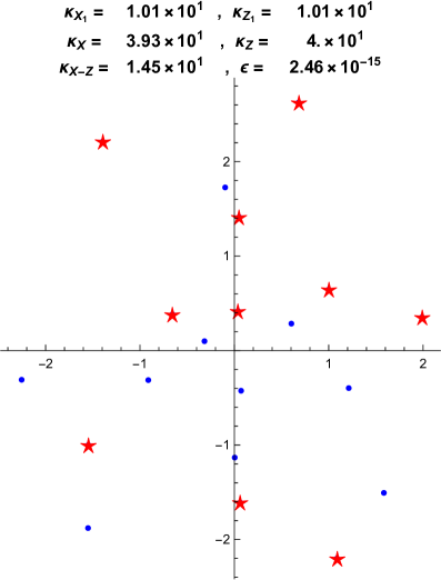
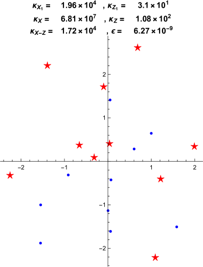
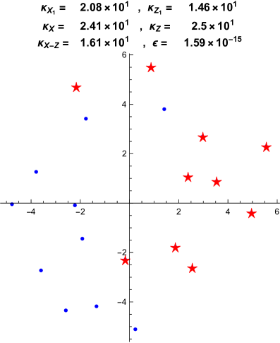
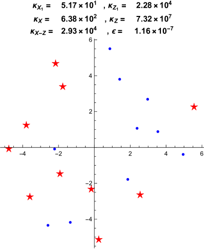
Figure 1. The best (left) and the worst (right) splittings of the spectrum of $\mathcal{C}_{1}$ from Example 4(a). The points of the spectrum of $\mathcal{C}_{1}$ related to $X$ are depicted by points, and related to $Z$ are depicted by stars

Figure 2. The best (left) and the worst (right) splittings of the spectrum of $\mathcal{C}_{1}$ from Example 4(b). The points of the spectrum of $\mathcal{C}_{1}$ related to $X$ are depicted by points, and related to $Z$ are depicted by stars

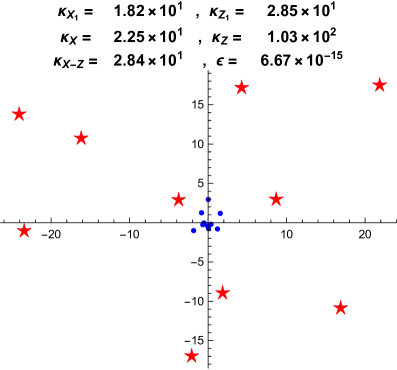
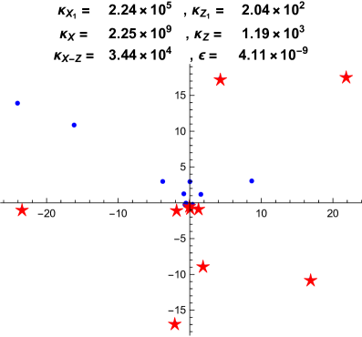
Figure 3. The best (left) and the worst (right) splittings of the spectrum of $\mathcal{C}_{1}$ from Example 4(c). The points of the spectrum of $\mathcal{C}_{1}$ related to $X$ are depicted by points, and related to $Z$ are depicted by stars

Example 4.

(a) We set $n=10$ and create matrices $B$ and $C$ consisting of random complex numbers uniformly distributed in $[-1,1]+[-i,i]$. We form the companion matrix $\mathcal{C}_{1}$ and find [37] its eigenvalues and eigenvectors. Since the matrices $B$ and $C$ are random, all eigenvalues are distinct and we obtain $2n=20$ different eigenvalues. We construct all splittings of the set $V$ of all normalized eigenvectors into two parts $V_{X}$ and $V_{Z}$, consisting of $n$ vectors. For each splitting, we create two block matrices

$$\begin{pmatrix}X_{1}\\ X_{2}\end{pmatrix},\qquad\begin{pmatrix}Z_{1}\\ Z_{2}\end{pmatrix},$$

whose columns are $V_{X}$ and $V_{Z}$ respectively. Then we pass to the matrices (if $X_{1}$ or $Z_{1}$ is not invertible or very badly invertible we exclude this splitting from the consideration)

$$\begin{pmatrix}\mathbf{1}\\ X\end{pmatrix}=\begin{pmatrix}X_{1}X_{1}^{-1}\\ X_{2}X_{1}^{-1}\end{pmatrix},\qquad\begin{pmatrix}\mathbf{1}\\ Z\end{pmatrix}=\begin{pmatrix}Z_{1}Z_{1}^{-1}\\ Z_{2}Z_{1}^{-1}\end{pmatrix}.$$

Thus, we associate a complete pair of right solvents $X$ and $Z$ with each splitting (Theorem 18). For each pair, we calculate the condition numbers

$$\varkappa(X_{1}),\;\varkappa(Z_{1}),\;\varkappa(X),\;\varkappa(Z),\;\varkappa(X-Z)$$

and the maximum $\varkappa_{\max}$ of these numbers. We select a complete pair of right solvents that corresponds to the smallest $\varkappa_{\max}$ and a complete pair of right solvents that corresponds to the largest $\varkappa_{\max}$; we call these pairs the best and the worst respectively.

We take $X_{1}$ and $X_{2}$ that correspond to the best pair. We create copies of $X_{1}$ and $X_{2}$ with 100 significant digits, adding zero digits at the end. We calculate $X$ and $Z$ again, and calculate the matrix (see Corollary 11)

$$U(1)=(e^{X}-e^{Z})(X-Z)^{-1}$$

with ordinary precision (about 16 significant digits) and with 100 significant digits; we denote the results by $U_{16}(1)$ and $U_{100}(1)$ respectively. We interpret $U_{100}(1)$ as the precise value. We calculate the relative error of $U(1)$

$$\varepsilon_{\text{best}}=\frac{\lVert U_{16}(1)-U_{100}(1)\rVert}{\lVert U_{16}(1)\rVert}$$

(for matrices, we use the norm induced by the Euclidian norm on $\mathbb{C}^{n}$).

We repeat the same calculations for the worst pair and denote the obtained number by $\varepsilon_{\text{worst}}$. The result of calculations is presented in Figure 2. We have repeated this experiment several times; the results are similar.

We also perform two modifications of this experiment: (b) with a matrix $B$ consisting of random complex numbers uniformly distributed in $[-1,1]+[-i,i]$ and a matrix $C$ consisting of random complex numbers uniformly distributed in $[-10,10]+[-10i,10i]$, see Figure 2; (c) with matrices $B$ and $C$ consisting of random complex numbers uniformly distributed in $[-10,10]+[-10i,10i]$, see Figure 3.

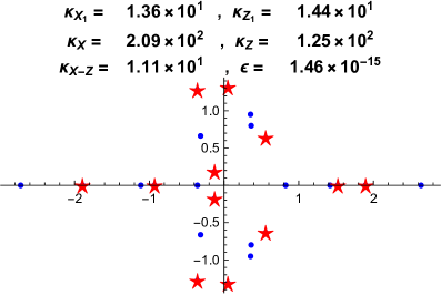
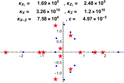
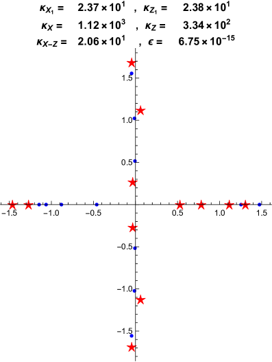
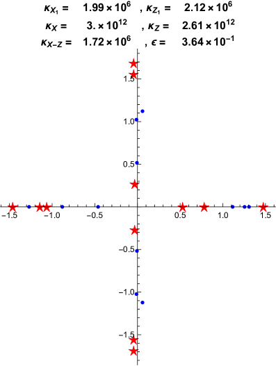
Figure 4. The best (left) and the worst (right) splittings of the spectrum of $\mathcal{C}_{1}$ from Example 5(a). The points of the spectrum of $\mathcal{C}_{1}$ related to $X$ are depicted by points, and related to $Z$ are depicted by stars

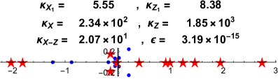
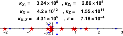
Figure 5. The best (left) and the worst (right) splittings of the spectrum of $\mathcal{C}_{1}$ from Example 5(b). The points of the spectrum of $\mathcal{C}_{1}$ related to $X$ are depicted by points, and related to $Z$ are depicted by stars

Figure 6. The best (left) and the worst (right) splittings of the spectrum of $\mathcal{C}_{1}$ from Example 5(c). The points of the spectrum of $\mathcal{C}_{1}$ related to $X$ are depicted by points, and related to $Z$ are depicted by stars

Example 5.

We consider a real selfadjoint pencil (i. e., the coefficients $B$ and $C$ are Hermitian matrices) [12, 13, 15, 16, 20, 21, 22, 30, 31, 32, 33].

(a) We set $n=12$ and create Hermitian matrices $B$ and $C$ (i. e., $B^{H}=B$ and $C^{H}=C$) consisting of random real numbers uniformly distributed in $[-1,1]$. We form the companion matrix $\mathcal{C}_{1}$ and find its eigenvalues and eigenvectors. All eigenvalues are distinct and we obtain $2n=24$ different eigenvalues. We recall that non-real eigenvalues occur in complex conjugate pairs. We construct all splittings of the set $V$ of all normalized eigenvectors into two parts $V_{X}$ and $V_{Z}$, consisting of $n$ vectors, such that if a complex eigenvalue $\lambda$ is related to $V_{X}$, then the conjugate number $\bar{\lambda}$ is also related to $V_{X}$. Taking into account only such splittings ensures that the solvents $X$ and $Z$ are real. After that we repeat the calculations from Example 4(a). The result is presented in Figure 6.

We perform two modifications of this experiment: (b) with a matrix $B$ consisting of random real numbers uniformly distributed in $[-0.1,0.1]$ and a matrix $C$ consisting of random real numbers uniformly distributed in $[-1,1]$, see Figure 6; (c) with a matrix $B$ consisting of random real numbers uniformly distributed in $[-1,1]$ and a matrix $C$ consisting of random real numbers uniformly distributed in $[-0.1,0.1]$, see Figure 6.

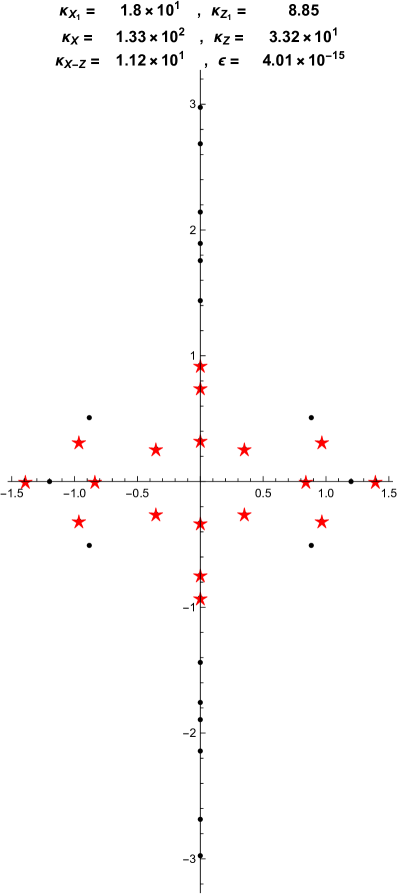
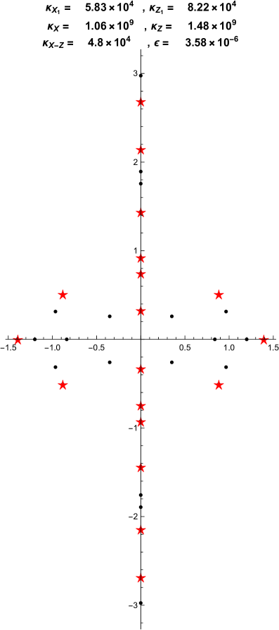
Figure 7. The best (left) and the worst (right) splittings of the spectrum of $\mathcal{C}_{1}$ from Example 6(a). The points of the spectrum of $\mathcal{C}_{1}$ related to $X$ are depicted by points, and related to $Z$ are depicted by stars

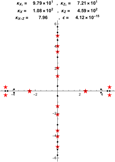
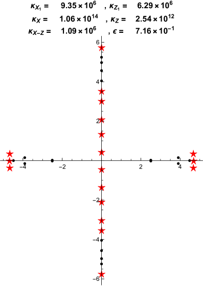
Figure 8. The best (left) and the worst (right) splittings of the spectrum of $\mathcal{C}_{1}$ from Example 6(b). The points of the spectrum of $\mathcal{C}_{1}$ related to $X$ are depicted by points, and related to $Z$ are depicted by stars

Example 6.

We consider a pencil corresponding to canonical differential equation [2, 6, 18, 19, 23, 34], [38, ch. II, § 3.2]. Such equations describe gyroscopic systems. Namely, we assume that $B$ and $C$ are real, $C$ is Hermitian and $B$ is skew-Hermitian ($B^{H}=-B$). In this case, the spectrum of $\mathcal{C}_{1}$ is symmetric with respect to both the real and imaginary axes. So, it is natural to put all symmetric pairs of eigenvalues into the same parts.

(a) We set $n=18$ and create a skew-Hermitian matrix $B$ and a Hermitian matrix $C$ (i. e., $B^{H}=-B$ and $C^{H}=C$) consisting of random real numbers uniformly distributed in $[-1,1]$. We form the companion matrix $\mathcal{C}_{1}$ and find its eigenvalues and eigenvectors. All eigenvalues are distinct and we obtain $2n=36$ different eigenvalues. We construct all splittings of the set $V$ of all normalized eigenvectors into two parts $V_{X}$ and $V_{Z}$, consisting of $n$ vectors, such that if an imaginary eigenvalue $\lambda$ is related to $V_{X}$, then the conjugate eigenvalue $\bar{\lambda}$ is also related to $V_{X}$, and if a real eigenvalue $\lambda$ is related to $V_{X}$, then the opposite eigenvalue $-\lambda$ is also related to $V_{X}$, and if a proper (i. e., with both $\operatorname{Re}\lambda\neq 0$ and $\operatorname{Im}\lambda\neq 0$) complex eigenvalue $\lambda$ is related to $V_{X}$, then the other three eigenvalues $-\lambda$, $\bar{\lambda}$, and $-\bar{\lambda}$ are also related to $V_{X}$. We repeat the calculations from Example 4(a). The result is presented in Figure 7.

Then we perform a modification of this experiment: (b) with a matrix $B$ consisting of random real numbers uniformly distributed in $[-1,1]$ and a matrix $C$ consisting of random real numbers uniformly distributed in $[-10,10]$, see Figure 8.

Numerical experiments carried out show that the relative error $\varepsilon_{\text{worst}}$ in $U(1)$ for the worst complete pair can be noticeably greater than the relative error $\varepsilon_{\text{best}}$ in $U(1)$ for best complete pair (especially, see Figures 6 and 8). It is also worth noticing that the large relative error $\varepsilon$ is more likely associated with large $\varkappa(X)$ or $\varkappa(Z)$ than large $\varkappa(X-Z)$. Some authors restrict themselves to searching for a dominant solvent, i.e., a solvent that corresponds to the largest eigenvalues in absolute value. Figures 2, 3, and 7 confirm that such a kind of solvents may lead to a good complete pair. Nevertheless, the remaining examples show that in general there is no simple connection between a good complete pair and a special type of splitting of the spectrum of $\mathcal{C}_{1}$ into two parts.

References

- [1] G. J. Davis. Numerical solution of a quadratic matrix equation. SIAM J. Sci. Statist. Comput., 2(2):164–175, 1981.
- [2] R. J. Duffin. The Rayleigh-Ritz method for dissipative or gyroscopic systems. Quart. Appl. Math., 18:215–221, 1960/61.
- [3] F. R. Gantmacher. The theory of matrices, volume 1. AMS Chelsea Publishing, Providence, RI, 1959.
- [4] I. Gohberg, P. Lancaster, and L. Rodman. Matrix polynomials. Academic Press, Inc. [Harcourt Brace Jovanovich, Publishers], New York-London, 1982. Computer Science and Applied Mathematics.
- [5] G. H. Golub and Ch. F. Van Loan. Matrix computations. Johns Hopkins Studies in the Mathematical Sciences. Johns Hopkins University Press, Baltimore, MD, third edition, 1996.
- [6] C.-H. Guo. Numerical solution of a quadratic eigenvalue problem. Linear Algebra Appl., 385:391–406, 2004.
- [7] C.-H. Guo, N. J. Higham, and F. Tisseur. Detecting and solving hyperbolic quadratic eigenvalue problems. SIAM J. Matrix Anal. Appl., 30(4):1593–1613, 2008/09.
- [8] N. J. Higham. Stable iterations for the matrix square root. Numer. Algorithms, 15(2):227–242, 1997.
- [9] N. J. Higham. Functions of matrices: theory and computation. Society for Industrial and Applied Mathematics (SIAM), Philadelphia, PA, 2008.
- [10] N. J. Higham and H.-M. Kim. Numerical analysis of a quadratic matrix equation. IMA J. Numer. Anal., 20(4):499–519, 2000.
- [11] N. J. Higham and H.-M. Kim. Solving a quadratric matrix equation by Newton’s method with exact line searches. SIAM J. Matrix Anal. Appl., 23(2):303–316 (electronic), 2001.
- [12] M. V. Keldysh. On the characteristic values and characteristic functions of certain classes of non-self-adjoint equations. Doklady Akad. Nauk SSSR (N. S.), 77(1):11–14, 1951. (in Russian).
- [13] M. V. Keldysh. The completeness of eigenfunctions of certain classes of nonselfadjoint linear operators. Uspehi Mat. Nauk, 26(4(160)):15–41, 1971. (in Russian); English translation in Russian Math. Surveys, 26(4):15–44 (1971).
- [14] I. D. Kostrub. Hamilton–Cayley theorem and the representation of the resolvent. Funktsional. Anal. i Prilozhen., 57(4):130–132, 2023. (in Russian).
- [15] M. G. Kreĭn and H. Langer. On some mathematical principles in the linear theory of damped oscillations of continua. I. Integral Equations Operator Theory, 1(3):364–399, 1978.
- [16] M. G. Kreĭn and H. Langer. On some mathematical principles in the linear theory of damped oscillations of continua. II. Integral Equations Operator Theory, 1(4):539–566, 1978.
- [17] I. V. Kurbatova. Functional calculus generated by a quadratic pencil. Zap. Nauchn. Sem. POMI, 389:113–130, 2011. (in Russian); English translation in J. Math. Sci., 182 (2012), no. 5, 646–655.
- [18] P. Lancaster. Lambda-matrices and vibrating systems, volume 94 of International Series of Monographs in Pure and Applied Mathematics. Pergamon Press, Oxford-New York-Paris, 1966.
- [19] P. Lancaster. Strongly stable gyroscopic systems. Electron. J. Linear Algebra, 5:53–66, 1999.
- [20] H. Langer. Über stark gedämpfte Scharen im Hilbertraum. J. Math. Mech., 17:685–705, 1967/68.
- [21] H. Langer. Factorization of operator pencils. Acta Sci. Math. (Szeged), 38(1-2):83–96, 1976.
- [22] A. S. Markus. Introduction to the spectral theory of polynomial operator pencils, volume 71 of Translations of Mathematical Monographs. American Mathematical Society, Providence, RI, 1988.
- [23] V. Mehrmann and D. Watkins. Structure-preserving methods for computing eigenpairs of large sparse skew-Hamiltonian/Hamiltonian pencils. SIAM J. Sci. Comput., 22(6):1905–1925, 2000.
- [24] A. N. Michel and Ch. J. Herget. Applied algebra and functional analysis. Dover Publications, Inc., New York, 1993.
- [25] M. A. Naĭmark. Normed algebras. Wolters-Noordhoff Series of Monographs and Textbooks on Pure and Applied Mathematics. Wolters-Noordhoff Publishing, Groningen, third edition, 1972.
- [26] A. I. Perov and I. D. Kostrub. Differentail equations in Banach algebras. Dokl. Akad. Nauk, 491(1):73–77, 2020.
- [27] A. I. Perov and I. D. Kostrub. On differential equations in Banach algebras. VGU Publishing House, Voronezh, 2020. (in Russian).
- [28] W. Rudin. Functional analysis. McGraw-Hill Series in Higher Mathematics. McGraw-Hill Book Co., New York–Düsseldorf–Johannesburg, first edition, 1973.
- [29] G. E. Shilov. Linear algebra. Dover Publications, Inc., New York, English edition, 1977.
- [30] A. A. Shkalikov. Strongly damped operator pencils and the solvability of the corresponding operator-differential equations. Mat. Sb. (N.S.), 135(177)(1):96–118, 1988. (in Russian); English translation in Math. USSR-Sb., 63(1):97–119, 1992.
- [31] A. A. Shkalikov. Operator pencils arising in elasticity and hydrodynamics: The instability index formula. In I. Gohberg, P. Lancaster, and P. N. Shivakumar, editors, Recent Developments in Operator Theory and Its Applications, pages 358–385, Basel, 1996. Birkhäuser Basel.
- [32] A. A. Shkalikov. Factorization of elliptic pencils and the Mandelstam hypothesis. In Contributions to operator theory in spaces with an indefinite metric (Vienna, 1995), volume 106 of Oper. Theory Adv. Appl., pages 355–387. Birkhäuser, Basel, 1998.
- [33] A. A. Shkalikov and V. T. Pliev. Compact perturbations of strongly damped operator pencils. Math. Notes, 45(2):167–174, 1989.
- [34] F. Tisseur and K. Meerbergen. The quadratic eigenvalue problem. SIAM Rev., 43(2):235–286, 2001.
- [35] J. S. H. Tsai, C. M. Chen, and L. S. Shieh. A computer-aided method for solvents and spectral factors of matrix polynomials. Applied mathematics and computation, 47(2-3):211–235, 1992.
- [36] Ch. F. Van Loan. The sensitivity of the matrix exponential. SIAM J. Numer. Anal., 14(6):971–981, 1977.
- [37] S. Wolfram. The Mathematica book. Wolfram Media, New York, fifth edition, 2003.
- [38] V. A. Yakubovich and V. M. Starzhinskii. Linear differential equations with periodic coefficients. 1, 2. Halsted Press [John Wiley & Sons], New York–Toronto, 1975.