Chebyshev Polynomial-Based Kolmogorov-Arnold Networks:
An Efficient Architecture for Nonlinear Function Approximation
Abstract
Accurate approximation of complex nonlinear functions is a fundamental challenge across many scientific and engineering domains. Traditional neural network architectures often struggle to capture intricate patterns and irregularities present in high-dimensional functions. This paper introduces the Chebyshev Kolmogorov-Arnold Network (Chebyshev KAN), a novel approach that combines the theoretical foundations of the Kolmogorov-Arnold Theorem with the powerful approximation capabilities of Chebyshev polynomials.
1 Introduction
The ability to accurately approximate complex nonlinear functions is a fundamental challenge in many areas of science, engineering, and artificial intelligence. Traditional neural network architectures, while powerful, often struggle to capture intricate patterns and irregularities in high-dimensional functions. This paper introduces a novel approach called the Chebyshev Kolmogorov-Arnold Network (Chebyshev KAN), which leverages theoretical principles from approximation theory to construct efficient neural network layers tailored for nonlinear function approximation. The core idea behind the Chebyshev KAN is to combine the Kolmogorov-Arnold Theorem from approximation theory [2, 3, 4]with the powerful approximation capabilities of Chebyshev polynomials. The Kolmogorov-Arnold Theorem states that any continuous multivariate function on a bounded domain can be represented as a superposition (composition) of a limited number of univariate functions and a set of linear operations. This theorem provides a theoretical foundation for approximating complex functions by breaking them down into simpler components. Chebyshev polynomials, on the other hand, are a sequence of orthogonal polynomials that exhibit excellent properties for function approximation, such as uniform convergence, rapid convergence, and efficient recursive computation. By combining the Kolmogorov-Arnold Theorem’s theoretical guarantee with the approximation power of Chebyshev polynomials, the Chebyshev KAN offers a principled and efficient approach to nonlinear function approximation. The paper provides a detailed mathematical explanation of the implementation of the Chebyshev KANs and the results of various experiments we conducted.
1.1 Kolmogorov-Arnold Theorem
The Kolmogorov-Arnold Theorem, also known as the Superposition Theorem or the Kolmogorov-Arnold Representation Theorem, is a fundamental result in approximation theory. It states that any continuous multivariate function on a bounded domain can be represented as a superposition (composition) of a limited number of one-variable (univariate) functions and a set of linear operations.
Formally, for a continuous function on the -dimensional unit hypercube , the Kolmogorov-Arnold Theorem guarantees the existence of continuous univariate functions and such that:
| (1) |
where .
1.2 Chebyshev Polynomials
Chebyshev polynomials are a sequence of orthogonal polynomials that play a crucial role in approximation theory[10, 11, 7] and numerical analysis. They are defined on the interval and satisfy the recurrence relation:
| (2) | ||||
| (3) | ||||
| (4) |
The first few Chebyshev polynomials are:
| (5) | ||||
| (6) | ||||
| (7) | ||||
| (8) | ||||
| (9) |
Chebyshev polynomials have several desirable properties that make them well-suited for function approximation:
-
•
Orthogonality: The Chebyshev polynomials are orthogonal with respect to the weight function on the interval . This property ensures that the coefficients in the polynomial approximation are uncorrelated, which can improve numerical stability and convergence.
-
•
Uniform Approximation: Chebyshev polynomials provide a uniform approximation of continuous functions on the interval . This means that the maximum approximation error is minimized compared to other polynomial approximations of the same degree.
-
•
Rapid Convergence: The approximation error of a continuous function using Chebyshev polynomials decreases rapidly as the degree of the polynomials increases, typically faster than other polynomial bases.
-
•
Recursive Computation: The recurrence relation for Chebyshev polynomials allows for efficient computation and evaluation, which is particularly advantageous in numerical implementations.
These properties make Chebyshev polynomials an excellent choice for function approximation tasks
1.3 The Chebyshev Kolmogorov-Arnold Network
The Chebyshev Kolmogorov-Arnold Network (Chebyshev KAN) is a novel approach to function approximation[4, 6], combining the theoretical foundations of the Kolmogorov-Arnold Theorem with the powerful approximation capabilities of Chebyshev polynomials.
In the Chebyshev KAN, the target multivariate function is approximated using a single layer of Chebyshev interpolation:
| (10) |
where is the normalized input tensor, is the -th Chebyshev polynomial evaluated at , is the degree of the Chebyshev polynomials, and are the learnable coefficients for the Chebyshev interpolation.
This formulation approximates the target function directly as a weighted sum of Chebyshev polynomials, leveraging the Kolmogorov-Arnold Theorem’s guarantee of the existence of a superposition of univariate functions to represent any continuous multivariate function.
2 The Chebyshev Kolmogorov-Arnold Network Layer
The Chebyshev Kolmogorov-Arnold Network (Chebyshev KAN) layer is a novel approach to function approximation, inspired by the Kolmogorov-Arnold Theorem and leveraging the expressive capabilities of Chebyshev polynomials. This section provides a detailed mathematical explanation of the Chebyshev KAN layer implementation, including tensor operations and illustrative examples.
2.1 Input Normalization
Since Chebyshev polynomials are defined on the interval , the first step in the Chebyshev KAN layer’s forward pass is to normalize the input tensor to this range, where is the batch size, and is the input dimension. This is achieved by applying the hyperbolic tangent function element-wise to the input tensor:
For example, consider an input tensor with shape , representing two input samples with two features each:
Applying the hyperbolic tangent function element-wise, we obtain the normalized input tensor :
By normalizing the input tensor, we ensure that the subsequent computations involving Chebyshev polynomials are well-defined and accurately capture the function approximation within the interval.
2.2 Chebyshev Polynomial Computation
After normalizing the input tensor, the next step is to compute the values of the Chebyshev polynomials up to the specified degree for each input dimension and batch sample[8, 9]. This computation is performed using the recurrence relation for Chebyshev polynomials:
To compute the Chebyshev polynomials, we initialize a tensor to store the values of the polynomials for each input dimension and batch sample. The first two columns of this tensor are initialized with the constant term and the first-degree term , respectively:
The remaining columns of are computed recursively using the recurrence relation:
where denotes the element-wise product between tensors. For example, let’s assume we want to compute the Chebyshev polynomials up to degree . The computation would proceed as follows:
After these computations, the tensor will contain the values of the Chebyshev polynomials , , , and for each input dimension and batch sample:
This tensor will be used in the next step to compute the Chebyshev interpolation and approximate the target function.
2.3 Chebyshev Interpolation
The final step in the Chebyshev KAN layer’s forward pass is to compute the Chebyshev interpolation, which is the weighted sum of the Chebyshev polynomials using the learnable coefficients . The Chebyshev interpolation is computed as follows:
where is the output tensor representing the approximation of the target function, and denotes the element-wise product between tensors.
To better understand this computation, let’s consider an example with (two input dimensions), (one output dimension), and (Chebyshev polynomials up to degree 2). The learnable coefficients could be:
The Chebyshev interpolation would then be computed as:
In this example, the Chebyshev KAN layer approximates the target function by computing a weighted sum of the Chebyshev polynomials up to degree 2, using the learnable coefficients . The resulting output tensor has shape , representing the approximated function values for the two input samples. The key steps in this computation are:
Compute the element-wise product for each input dimension and polynomial degree . This gives the weighted Chebyshev polynomial values for each input dimension and output dimension. Sum the weighted Chebyshev polynomial values across input dimensions and degrees to obtain the final approximation .
By learning the appropriate values of the coefficients during the training process, the Chebyshev KAN layer can approximate a wide range of continuous functions, as guaranteed by the Kolmogorov-Arnold Theorem.
2.4 Training and Optimization
The Chebyshev KAN layer is trained by optimizing the learnable coefficients to minimize a loss function between the predicted output and the true output :
where is a suitable loss function (e.g., mean squared error for regression tasks, cross-entropy for classification tasks), and is the batch size. The gradients[14] of the loss with respect to the learnable coefficients are computed using backpropagation:
The partial derivative can be computed using the chain rule and the Chebyshev interpolation formula:
Once the gradients are computed, the coefficients are updated using an optimization algorithm, such as stochastic gradient descent (SGD) or its variants:
where is the learning rate. This training process is repeated for multiple epochs, iterating over [1, 16]the training dataset and updating the coefficients to minimize the loss function and improve the approximation of the target function. The Chebyshev KAN can be applied to various function approximation tasks, including regression, classification, and time series forecasting, across diverse domains such as finance, physics, engineering, and computational biology. It is particularly suitable for scenarios where the target function exhibits complex nonlinear behavior and traditional neural network architectures struggle to capture the underlying patterns accurately.
Additionally, the Chebyshev KAN layer can be incorporated into more complex neural network architectures, such as convolutional neural networks or recurrent neural networks, to enhance their function approximation capabilities for specific applications.
2.5 Ablation Studies
In this study, we conducted ablation experiments to evaluate the impact of various factors on the performance of the Chebyshev Kolmogorov-Arnold Network (Chebyshev KAN) model for the task of image classification on the MNIST dataset[15]. The model architecture used in these experiments consists of three Chebyshev KAN layers followed by Layer Normalization layers to avoid gradient vanishing caused by the tanh activation function[12]. The model’s hyperparameters, such as the degree of Chebyshev polynomials and the type of input normalization, were systematically varied to assess their influence on the model’s accuracy.
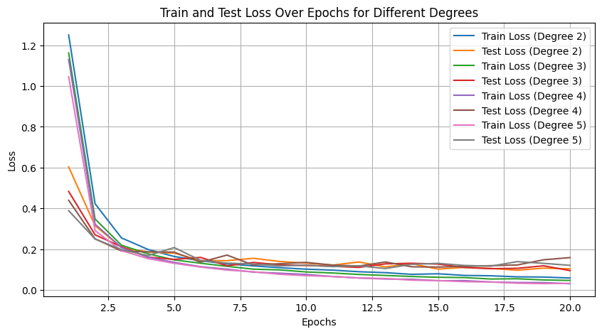
2.5.1 Degree of Chebyshev Polynomials
We investigated the effect of varying the degree of Chebyshev polynomials on the model’s accuracy. The degree determines the complexity of the polynomial approximation used in the Chebyshev KAN layer. We experimented with degrees ranging from 2 to 5 and observed the resulting accuracy on the MNIST test set. The results, presented in Table 1, indicate that increasing the degree generally improves accuracy up to a certain point.
| Degree | Accuracy | Total Trainable Parameters |
|---|---|---|
| 2 | 0.9697 | 77,376 |
| 3 | 0.9718 | 103,136 |
| 4 | 0.9553 | 128,896 |
| 5 | 0.9646 | 154,656 |
As shown in Table 1, increasing the degree of Chebyshev polynomials from 2 to 3 leads to a slight improvement in accuracy, while further increasing the degree to 4 results in a significant drop in performance. Finally, increasing the degree to 5 yields a modest improvement in accuracy compared to a degree of 2 polynomial, but it is still lower than the accuracy achieved with a degree 3 polynomial. This observation suggests that a polynomial of degree 3 offers a good balance between model complexity and generalization ability for the MNIST dataset.
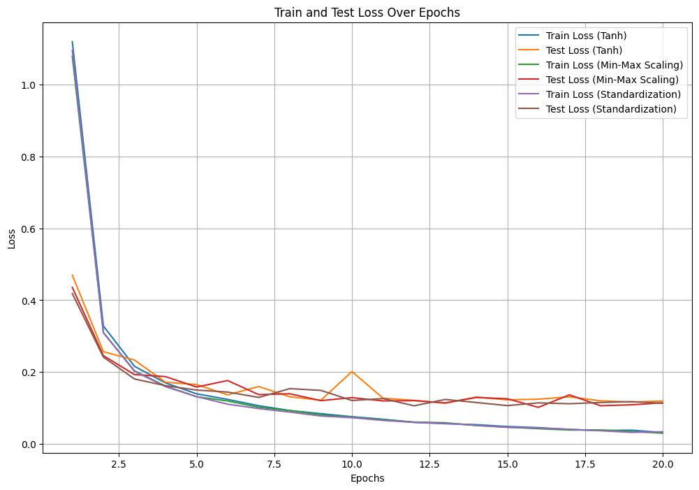
2.5.2 Input Normalization
We also investigated the effect of different input normalization techniques on the model’s accuracy. We compared the performance of the MNIST-KAN model when using tanh normalization, Min-Max Scaling, and Standardization. The results, presented in Table 2, indicate that tanh normalization and Min-Max Scaling achieve similar accuracy, while Standardization performs slightly better.
| Normalization | Accuracy |
|---|---|
| Tanh | 0.9680 |
| Min-Max Scaling | 0.9683 |
| Standardization | 0.9692 |
In Table 2, we can observe that tanh normalization and Min-Max Scaling yield comparable results, with both achieving an accuracy of around 96.8%. This suggests that these normalization techniques are effective in preprocessing the input data for the Chebyshev KAN model. However, Standardization outperforms both tanh normalization and Min-Max Scaling, achieving an accuracy of 96.92%.
3 Experiments and Results
In this section, we evaluate the performance of the Chebyshev Kolmogorov-Arnold Network (Chebyshev KAN) model on a complex fractal-like 2D function[17]. The experiments are designed to assess the model’s ability to capture intricate patterns and irregularities in high-dimensional functions, which is a fundamental challenge in many areas of science, engineering, and artificial intelligence.
3.1 Fractal-like 2D Function
To further evaluate the performance of the Chebyshev KAN model on complex functions, we generated a fractal-like 2D function using a combination of trigonometric functions, absolute values, and noise. The fractal function is defined as follows:
def fractal_function(x, y):
    z = np.sin(10 * np.pi * x) * np.cos(10 * np.pi * y) + np.sin(np.pi * (x**2 + y**2))
    z += np.abs(x - y) + (np.sin(5 * x * y) / (0.1 + np.abs(x + y)))
    z *= np.exp(-0.1 * (x**2 + y**2))

    # Add noise to z
    noise = np.random.normal(0, 0.1, z.shape)
    z += noise
    return z
We created a dataset by uniformly sampling 100 points in the range for both and , resulting in a grid of function values from the fractal_function. The dataset was not explicitly split into training and testing sets in the provided code.
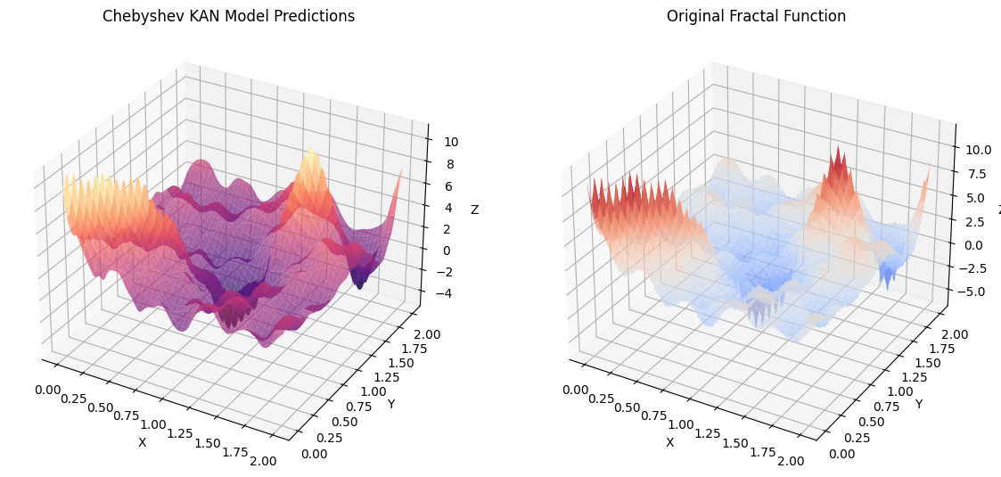
The ChebyKAN model has three layers that transform the input data step-by-step. The first layer takes the 2D input coordinates and maps them to 8 output features using Chebyshev polynomials of degree 8. This allows capturing complex patterns in the input. The second layer takes the 8 output features from the first layer and maps them to 16 output features using Chebyshev polynomials of a lower degree 4, refining the learned representation. The third and final layer takes the 16 output features from the second layer and maps them to a single output, which is the predicted function value, using Chebyshev polynomials of degree 4. The degree of the Chebyshev polynomials in each layer controls the complexity of the mapping function learned. Higher degrees allow more complex mappings but increase the risk of overfitting. We trained the Chebyshev KAN model for 2,000 epochs using the Adam optimizer with a learning rate of 0.01. The losses obtained during the training process of ChebyKAN models were recorded.
Figure 2 shows the predictions of the Chebyshev KAN model for the fractal-like 2D function. The model successfully captures the intricate patterns and irregularities present in the function, demonstrating its ability to approximate complex high-dimensional functions.
In summary, tests on a complex 2D function showed that the Chebyshev KAN model is very good at understanding complicated patterns and details in functions with many dimensions. The model did really well with a dataset of a fractal-like 2D function, showing it has a lot of promise for tasks that involve estimating functions in various areas. In the future, researchers might look into using different ways to adjust the model or combining several methods to make it even better. Also, combining the Chebyshev KAN model with more complex types of neural networks, like those used for image recognition or processing language, could lead to new and innovative ways to estimate functions. This could be useful in a wide range of fields, including computer vision, language understanding, and creating new content.
4 Future Directions
While the Chebyshev KAN layer presents a promising approach to function approximation, several avenues for further research and development remain:
-
•
Alternative Basis Functions: Exploring alternative basis functions or combinations of basis functions, beyond Chebyshev polynomials, could potentially lead to improved approximation accuracy or computational efficiency for certain classes of functions.
-
•
Adaptive Degree Selection: Developing techniques for automatically determining the appropriate degree of Chebyshev polynomials or other basis functions based on the complexity of the target function could enhance the flexibility and generalization capabilities of the Chebyshev KAN layer.
-
•
Regularization and Training Strategies: Investigating effective regularization techniques and training strategies tailored to the Chebyshev KAN layer’s architecture could improve convergence, generalization, and robustness in practical applications.
-
•
Integration with Other Neural Network Architectures: Combining the Chebyshev KAN layer with other neural network architectures, such as attention mechanisms or generative models, could lead to novel hybrid approaches for function approximation and open up new applications in fields like computer vision, natural language processing, and generative modeling.
-
•
Theoretical Analysis: Conducting further theoretical analyses of the Chebyshev KAN layer’s approximation properties, computational complexity, and convergence behavior could provide valuable insights and guide future developments in this area.
Overall, the Chebyshev KAN layer represents a promising step towards leveraging theoretical foundations and efficient approximation techniques in the field of machine learning, paving the way for more interpretable and resource-efficient function approximation models.
A significant amount of research is currently being conducted in the field of function approximation using the Kolmogorov-Arnold Network (KAN) architecture. The KAN offers a promising alternative to traditional Multi-Layer Perceptron (MLP) models, with the added advantage of increased interpretability due to its theoretical foundations in the Kolmogorov-Arnold Theorem and the use of Chebyshev polynomials as a basis for approximation. The flexibility and principled approach of the KAN architecture open up numerous possibilities for its integration into various neural network architectures, such as Transformers, Convolutional Neural Networks (CNNs), and others. Researchers are actively exploring the development of KAN-based architectures tailored for diverse applications across various domains. As research in this area continues to progress, the KAN has the potential to emerge as a formidable rival to the widely-used MLP, offering a more interpretable and resource-efficient solution for nonlinear function approximation tasks. We have implemented the Chebyshev KAN in a publicly available Python package hosted on the Python Package Index (PyPI): https://pypi.org/project/Deep-KAN/.
References
- [1] Rossi, F., & Conan-Guez, B. (2005). Functional multi-layer perceptron: a non-linear tool for functional data analysis. Neural Netw, 18(1), 45-60. doi: 10.1016/j.neunet.2004.07.001. PMID: 15649661.
- [2] Liu, Z., Wang, Y., Vaidya, S., Ruehle, F., Halverson, J., Soljačić, M., Hou, T. Y., & Tegmark, M. (2024). KAN: Kolmogorov-Arnold Networks. ArXiv. https://arxiv.org/abs/2404.19756
- [3] Rivlin, T. J. (1974). Chapter 2, Extremal properties. In The Chebyshev Polynomials. Pure and Applied Mathematics (1st ed.). New York-London-Sydney: Wiley-Interscience [John Wiley Sons]. pp. 56–123. ISBN 978-047172470-4.
- [4] Schmidt-Hieber, J. (2021). The Kolmogorov–Arnold representation theorem revisited. Neural Networks, 137, 119-126. https://doi.org/10.1016/j.neunet.2021.01.020
- [5] Goldman, R. (2002). B-Spline Approximation and the de Boor Algorithm. Pyramid Algorithms, 347-443. https://doi.org/10.1016/B978-155860354-7/50008-8
- [6] Braun, J., Griebel, M. (2009). On a constructive proof of Kolmogorov’s superposition theorem. Constructive Approximation, 30(3), 653–675. doi:10.1007/s00365-009-9054-2.
- [7] Chebyshev, P. L. (1854). ”Théorie des mécanismes connus sous le nom de parallélogrammes”. Mémoires des Savants étrangers présentés à l’Académie de Saint-Pétersbourg (in French), 7, 539–586.
- [8] Glimm, J. (1960). ”A Stone–Weierstrass Theorem for C*-algebras”. Annals of Mathematics. Second Series, 72(2), 216–244 [Theorem 1]. doi:10.2307/1970133. JSTOR 1970133.
- [9] Dragomir, S. S. (2003), ”A survey on Cauchy–Bunyakovsky–Schwarz type discrete inequalities”, Journal of Inequalities in Pure and Applied Mathematics, 4(3), 142 pages, archived from the original on 2008-07-20.
- [10] Cesarano, C., and Ricci, P. E. (2019). Orthogonality Properties of the Pseudo-Chebyshev Functions (Variations on a Chebyshev’s Theme). Mathematics, 7(2), 180. https://doi.org/10.3390/math7020180
- [11] Karageorghis, A. (1987). A note on the Chebyshev coefficients of the general order derivative of an infinitely differentiable function. Journal of Computational and Applied Mathematics, 21(1), 129-132. https://doi.org/10.1016/0377-0427(88)90396-2
- [12] Dubey, S. R., Singh, S. K., Chaudhuri, B. B. (2021). Activation Functions in Deep Learning: A Comprehensive Survey and Benchmark. ArXiv. https://arxiv.org/abs/2109.14545
- [13] Riechers, P. M. (2024). Geometry and Dynamics of LayerNorm. ArXiv. https://arxiv.org/abs/2405.04134
- [14] Hochreiter, S.; Bengio, Y.; Frasconi, P.; Schmidhuber, J. (2001). ”Gradient flow in recurrent nets: the difficulty of learning long-term dependencies”. In Kremer, S. C.; Kolen, J. F. (eds.). A Field Guide to Dynamical Recurrent Neural Networks. IEEE Press. ISBN 0-7803-5369-2.
- [15] Deng, L. (2012). The MNIST Database of Handwritten Digit Images for Machine Learning Research [Best of the Web]. IEEE Signal Processing Magazine, 29(6), 141-142. https://doi.org/10.1109/MSP.2012.2211477
- [16] Goodfellow, I.; Bengio, Y.; Courville, A. (2016). Deep Learning. MIT Press. http://www.deeplearningbook.org/
- [17] SynodicMonth. ChebyKAN. GitHub repository. Retrieved from https://github.com/SynodicMonth/ChebyKAN.