Optimal Trade Characterizations in Multi-Asset Crypto-Financial Markets

Abstract. This work focuses on the mathematical study of constant function market makers. We rigorously establish the conditions for optimal trading under the assumption of a quasilinear, but not necessarily convex (or concave), trade function. This generalizes previous results that used convexity, and also guarantees the robustness against arbitrage of so-designed automatic market makers. The theoretical results are illustrated by families of examples given by generalized means, and also by numerical simulations in certain concrete cases. These simulations along with the mathematical analysis suggest that the quasilinear-trade-function based automatic market makers might replicate the functioning of those based on convex functions, in particular regarding their resilience to arbitrage.

Keywords: Cryptofinance; Optimal trading; Decentralized markets, Automatic market makers; Nonconvex optimization; Quasiconvexity.

1 Introduction

Cryptocurrencies have had a deep impact in the XXIst century world. The Bitcoin white paper [30] has not only given rise to an asset which market price has grown to several dozens of thousands of dollars, but has also been cited tens of thousands of times. Its impact has then ranged from financial practice to academic research. The rise of cryptocurrencies has also generated a debate about how finance can be evolved accordingly. This is the starting point of the revolutionary decentralized finance (DeFi).

Automatic Market Makers (AMMs) have their own status within decentralized finance. The were born to provide an automated liquidity provision, along with trading services, on blockchain networks. Nowadays, some AMMs such as Uniswap [2], Balancer [27], and Curve [16] enjoy a huge popularity among practitioners. Their main functionality is to enable decentralized exchange (DEX) of digital assets. This, in turn, facilitates trading, lending, and yield farming.

An AMM is a smart contract protocol that permits to trade cryptoassets without the need of an order book. They are based on exchange algorithms that, together with liquidity pools, set the trading framework. Each algorithm determines how the corresponding AMM works, as it is responsible of tuning the asset prices, providing liquidity, and the market efficiency. Its functioning, in consequence, differs sharply from that of traditional centralized exchanges, which match the orders emitted by buyers and sellers.

Several advantages and disadvantages can be associated with AMMs. On the positive side, they are assumed to facilitate the democratization of financial markets. Any trader can execute exchanges according to what is set by the predetermined algorithm, or either deposit digital assets in the liquidity pools for a fee. Therefore, AMMs reduce the need to rely on intermediaries and counterpart risk if compared to centralized exchanges. Nevertheless, AMM users can also experience a number of negative aspects, such as impermanent loss, front-running, and slippage. The design of AMM protocols, and in particular of the exchange algorithms, is therefore key to improve their features and to diminish their handicaps.

This work is devoted to the construction of a general mathematical framework for the theoretical design of exchange algorithms. We depart from the model in [3] to consider the optimization:

$$\begin{array}[]{lll}&\text{maximize}&U(x-y)\\ &\text{subject to}&\varphi(R+\Gamma y-x)=\varphi(R)\text{, }\\ &&R+\Gamma y-x\geq 0\text{, }\\ &&R\geq x\geq 0\text{, }y\geq 0.\end{array}$$ (1.1)

Herein $U:\mathbb{R}^{n}\longrightarrow\mathbb{R}$ is the utility function that models the preferences of the trader (and which, of course, the trader seeks to maximize), $n$ is the number of cryptoassets, $x,y\in\mathbb{R}^{n}$ are the baskets of assets demanded from and sent to the AMM, respectively, $R$ are the reserves of the AMM, and $\Gamma$ is a $n\times n$ diagonal matrix that encodes the fees charged by the AMM to the trader for performing the trade. The function $\varphi:\mathbb{R}^{n}\longrightarrow\mathbb{R}$ is the one that controls the exchange algorithm, as it should kept constant at every trade; thus the name “constant function market maker” for this type of AMM [4] (see also [21]). The rest of the constraints are there to keep the non-negativity of the reserves and of the quantities of assets traded; note that the vectorial inequalities should be understood componentwise. In the case of Uniswap, for instance, the function $\varphi(\cdot)$ can be taken to be the geometric mean (or equivalently the product of the components). This case along with several generalizations and variants have been extensively studied in the literature, see for instance [4, 5, 6, 7], where this list is not meant to be exhaustive. We depart from these studies, and get inspired by them, and more particularly of [3], to carry out our analysis, which is actually a generalization of some instances of the latter work.

Our contribution: We provide necessary and sufficient optimality conditions for optimal trades in multi-asset crypto-financial markets beyond convexity, that is, when both trading and utility functions satisfy generalized convexity assumptions. This improvement is more than theoretical since it has economical/financial motivations for the potential development of new crypto-financial markets based on AMM algorithms. As it is well-known by the consumer preference theory [15], utility functions are naturally assumed quasiconcave because preferences that result in concave utility functions are often considered artificial (see, for instance, [15, 28]). Furthermore, we consider the trading function to be quasilinear, a generalized convexity assumption which includes the nonincreasing/nondecreasing convex (or concave) case, preserves the convexity of problem (1.1) and also the equality in the constraint without been restricted to the simple linear (affine) case. Moreover, the new optimality conditions that we establish are valid for any trade while, until now, only the no-trade case (when the optimal pair is $(0,0)$, i. e. it is best not to trade whatsoever) was known in the literature for the convex case [3]. Our proofs do not just cover the case of an uniform fee as assumed in [3], but also extend the analysis to the case of asset-dependent fees, which is a generalization that can be implemented in real AMMs. Finally, we apply our results to construct new trading functions that are generalized means. This obviously includes as particular cases the geometric and arithmetic means, which has been used in both academic articles and real AMMs. Nevertheless, our results include the case of quasilinear generalized means that are neither convex nor concave, which were not regarded in previous theoretical developments, and open the possibility to start the design of new AMMs built upon this new type of trading functions.

The paper is organized as follows. In section 2 we introduce the definitions and mathematical terminology that will be employed from there onwards. In section 3 we formulate the problem of optimal trading in an AMM as a mathematical optimization, making precise the above description. In section 4, the results of the previous section are employed to characterize the optimality of not executing any trade, that is, to characterize when no trading whatsoever is the optimal choice. This is important to establish the robustness of the AMM to the action of arbitrageurs, since under those conditions no trades will be executed just for the sake of profit. In section 5, we illustrate our theoretical developments with particular examples. We focus on the case in which the trade function is neither convex nor concave, something that escapes previous theoretical frameworks. We make these ideas concrete by employing generalized means, which we propose as trade functions, and combine theoretical and numerical analyses to assess them. Finally, in section 6, we draw our conclusions.

2 Preliminaries

We denote $\mathbb{R}_{+}:=[0,+\infty[$ and $\mathbb{R}_{++}:=\,]0,+\infty[$. Hence, $\mathbb{R}^{n}_{+}:=[0,+\infty[\,\times\ldots\times[0,+\infty[$ and $\mathbb{R}^{n}_{++}:=\,]0,+\infty[\times\ldots\times\,]0,+\infty[$ ($n$ times). We used the usual notations $\geq$ componentwise (see [17])

$$~{}~{}x\geq y~{}\Longleftrightarrow~{}x_{i}\geq y_{i},$$

$$~{}~{}x\gneq y~{}\Longleftrightarrow~{}x_{i}\geq y_{i},x\neq y,$$

$$x>>y~{}\Longleftrightarrow~{}x_{i}>y_{i},$$

for every $i=1,...,n$.

Let $K\subseteq\mathbb{R}^{n}$ be nonempty. Then the set $K^{\ast}\subseteq\mathbb{R}^{n}$ is the polar (positive) cone of $K$ defined by

$$K^{\ast}:=\{q\in\mathbb{R}^{n}:~{}\langle q,p\rangle\geq 0,~{}\forall~{}p\in K\}.$$ (2.1)

Given any extended-valued function $h:\mathbb{R}^{n}\rightarrow\overline{\mathbb{R}}:=\mathbb{R}\cup\{\pm\infty\}$, the effective domain of $h$ is defined by ${\rm dom}\,h:=\{x\in\mathbb{R}^{n}:h(x)<+\infty\}$. It is said that $h$ is proper if ${\rm dom}\,h$ is nonempty and $h(x)>-\infty$ for all $x\in\mathbb{R}^{n}$. The notion of properness is important when dealing with minimization problems.

It is indicated by ${\rm epi}\,h:=\{(x,t)\in\mathbb{R}^{n}\times\mathbb{R}:h(x)\leq t\}$ the epigraph of $h$, by $S_{\lambda}(h):=\{x\in\mathbb{R}^{n}:h(x)\leq\lambda\}$ (resp. $S^{<}_{\lambda}(h):=\{u\in\mathbb{R}^{n}:~{}h(u)<\lambda\}$ the sublevel (resp. strict sublevel) set of $h$ at the height $\lambda\in\mathbb{R}$, by $W_{\lambda}(h):=\{x\in\mathbb{R}^{n}:h(x)\geq\lambda\}$ (resp. $W^{<}_{\lambda}(h):=\{u\in\mathbb{R}^{n}:~{}h(u)>\lambda\}$ the upper level (resp. strict upper level) set of $h$ at the height $\lambda\in\mathbb{R}$, and by ${\rm argmin}_{\mathbb{R}^{n}}h$ the set of all minimal points of $h$.

A function $h$ with convex domain is said to be

• convex if, given any $x,y\in\mathrm{dom}\,h$, then

  $$h(\lambda x+(1-\lambda)y)\leq\lambda h(x)+(1-\lambda)h(y),~{}\forall~{}\lambda\in[0,1],$$ (2.2)

• quasiconvex if, given any $x,y\in\mathrm{dom}\,h$, then

  $$h(\lambda x+(1-\lambda)y)\leq\max\{h(x),h(y)\},~{}\forall~{}\lambda\in[0,1],$$ (2.3)

It is said that $h$ is strictly convex (resp. strictly quasiconvex) if the inequality in (2.2) (resp. (2.3)) is strict whenever $x\neq y$ and $\lambda\in\,]0,1[$. Every convex function is quasiconvex, but the reverse statement does not hold as the function $h(x)=x^{3}$ shows. Recall that

$$h~{}\mathrm{is~{}convex} \Longleftrightarrow\,\mathrm{epi}\,h~{}\mathrm{is~{}a~{}convex~{}set;}$$

$$h~{}\mathrm{is~{}quasiconvex} \Longleftrightarrow\,S_{\lambda}(h)~{}\mathrm{is~{}a~{}convex~{}set~{}for~{}all~{}}\lambda\in\mathbb{R}.$$

Quasiconvex functions appear in many applications from different fields as, for instance, in Economics and Financial Theory, especially in consumer preference theory (see [15, 28]), since quasiconcavity is the mathematical formulation of the natural assumption of a tendency to diversification on the consumers.

It is said that $h$ is quasilinear if $h$ is quasiconvex and $-h$ is quasiconvex. As a consequence, its sublevel set $S_{\lambda}(h)$ and its upper level sets $W_{\lambda}(h)$ are convex for all $\lambda\in\mathbb{R}$ (see [12, Theorem 3.3.1]). Note that every nonincreasing/nondecreasing convex (or concave) function is quasilinear, because all its sublevel and upper level sets are convex.

Let $K\subseteq\mathbb{R}^{n}$ be a convex set and $h:K\rightarrow\mathbb{R}$ be a differentiable function. Then the following assertions holds:

• $h$ is quasiconvex if and only if for every $x,y\in K$, we have (see [8] and [9, Theorem 3.11]) that

  $$h(x)\leq h(y)~{}\Longrightarrow~{}\langle\nabla h(y),x-y\rangle\leq 0;$$ (2.4)

• $h$ is quasilinear if and only if for every $x,y\in K$, we have (see [12, Theorem 3.3.6])

  $$h(x)=h(y)~{}\Longrightarrow~{}\langle\nabla h(y),x-y\rangle=0.$$ (2.5)

Let $h:\mathbb{R}^{n}\rightarrow\mathbb{R}$ be a differentiable function. Then $h$ is said to be pseudoconvex (see [26]) if

$$h(x)<h(y)~{}\Longrightarrow~{}\langle\nabla h(y),x-y\rangle<0.$$ (2.6)

A function $h$ is pseudoconcave if $-h$ is pseudoconvex.

If $h$ is pseudoconvex, then every local minimum is global minimum [12, Theorem 3.2.5] and, as a consequence, if $x$ is not a local minimum point of a pseudoconvex function $h$, then

$${\rm int}(S_{h(x)}(h))=S^{<}_{h(x)}(h).$$ (2.7)

Fur a further study on generalized convexity we refer to [9, 8, 12, 26, 34] among others.

3 The Optimization Problem

Based on [3], the following optimization problem, modeling how to choose a valid trade, is considered

$$\begin{array}[]{lll}(Q):&\text{maximize}&U(x-y)\\ &\text{subject to}&\varphi(R+\Gamma y-x)=\varphi(R)\text{, }R+\Gamma y-x\geq 0\text{, }R\geq x\geq 0\text{, }y\geq 0.\end{array}$$

Here $\varphi:\mathbb{R}^{n}_{+}\rightarrow\mathbb{R}_{+}$ is the trading function while $U:\mathbb{R}^{n}\rightarrow\mathbb{R}$ is the utility that the trader want to maximize, $x,y\in\mathbb{R}^{n}_{+}$ correspond with the given (tender) and the received basket. If fact, this model is a generalization of the model presented in [3], since it considers a diagonal matrix $\Gamma=\left\{\gamma_{i}\delta_{ij}\right\}_{1\leq i,j\leq n}$, here $\delta_{ij}$ is the usual Kronecker delta ($\delta_{ii}=1,$ $\delta_{ij}=1$ for $i\neq j$), the scalar $0<\gamma_{i}<1$ represent the positive discount rate to the asset $i$, while $R\in\mathbb{R}_{+}^{n}$ is the reserve of available assets. Without loss of generality, we assume that $R>0$ and

$$\nabla U(x)\geq 0,~{}\forall~{}x\in\mathbb{R}^{n},$$ (3.1)

$$\nabla\varphi(x)\gneq 0,~{}\forall~{}x>0.$$ (3.2)

Note that (3.2) implies that $\varphi$ is strictly increasing with respect to at least one component and, in particular,

$$x\geq y~{}\Longrightarrow~{}\varphi(x)\geq\varphi(y),~{}\forall~{}x,y>0.$$ (3.3)

We can rewritte the problem in the following abstract way

$$\begin{array}[]{lcc}(Q):&\text{maximize}&f(x,y)\\ &\text{s.t.}&h(x,y)=0\text{, }g(x,y)\leq 0,\text{ }\left(x,y\right)\in\hat{S}.\end{array}$$

where the maps $f,h:\mathbb{R}^{n}\times\mathbb{R}^{n}\rightarrow\mathbb{R}$, $g:\mathbb{R}^{n}\times\mathbb{R}^{n}\rightarrow\mathbb{R}^{n}$ and the convex set $\hat{S}$ are defined by

$$\begin{array}[]{l}f(x,y)=U(x-y),\\ h(x,y)=\varphi(R+\Gamma y-x)-\varphi(R),\\ g(x,y)=-R-\Gamma y+x,\\ \hat{S}=\{(x,y)\in\mathbb{R}^{n}\times\mathbb{R}^{n}:\text{ }R\geq x\geq 0\text{, }y\geq 0\}.\end{array}$$

This is an optimization problem with an equality and inequality contraint and convex contraints on the variable. While natural assumptions can be given to $U$ and $\varphi$, we will assume that the maps are continuously differentiable.

We first study the solvability of this problem in the general case when the objective map is continuous and the feasible set is nonvoid and compact, therefore there exists a solution $(\bar{x},\bar{y})$ to $(Q)$ by applying known results as, for instance, [23, Thr 2.3]. Furthermore we assume the following complementary condition on $(\bar{x},\bar{y})$

$$0\leq\bar{x}\bot\bar{y}\geq 0~{}\Longleftrightarrow~{}\bar{x}\geq 0,\,\bar{y}\geq 0\text{, }\bar{x}_{i}\bar{y}_{j}=0,~{}\forall~{}i=1,...,n.$$ (3.4)

In the context of our appplication, this is a natural assumption since it corresponds with the non-overlapping support of valid tender and receive baskets (see [3, Section 3]). In the following we understand that $U$ is strongly increasing when $x\gneq y$ implies $U(x)>U(y)$.

Proposition 3.1.

There exists a solution $(\bar{x},\bar{y})$ of $(Q)$. Furthermore, if $U$ is strongly increasing, then $0\leq\bar{x}\bot\bar{y}\geq 0$.

Note that in virtue of [3, Section 3], the complementary condition also justifies the constraint $x\leq R$ in $(Q)$.

3.1 Necessary Conditions

A necessary condition is given by a standard multiplier rule [23, Thr 5.3]: Assume $(\bar{x},\bar{y})$ solves problem $(Q)$. If the following property (Kurcyusz-Robinson-Zowe constraint qualification) is verified

$$\left(\begin{array}[]{c}\nabla g(\bar{x},\bar{y})\\ \nabla h(\bar{x},\bar{y})\end{array}\right)\operatornamewithlimits{cone}(\hat{S}-(\bar{x},\bar{y}))+\operatornamewithlimits{cone}\left(\begin{array}[]{c}\mathbb{R}_{+}^{n}+\left\{g(\bar{x},\bar{y})\right\}\\ 0\end{array}\right)=\mathbb{R}^{n}\times\mathbb{R},$$ (3.5)

then the following multiplier rule is verified: Find $(\bar{x},\bar{y},\mu,\lambda)\in\mathbb{R}^{n}\times\mathbb{R}^{n}\times\mathbb{R}_{+}^{n}\times\mathbb{R}$ such that

$$\begin{array}[]{l}\left(-\nabla f(\bar{x},\bar{y})+\mu^{T}\nabla g(\bar{x},\bar{y})+\lambda\nabla h(\bar{x},\bar{y})\right)(x-\bar{x},y-\bar{y})\geq 0\text{ for every }x,y\in\hat{S},\\ \mu^{T}g(\bar{x},\bar{y})\leq 0\\ h(\bar{x},\bar{y})=0.\end{array}$$ (3.6)

In the following result, we present a general necessary condition for complementary solutions of problem $(Q)$. In this sense, given $x\in\mathbb{R}^{n}$, we will use the notation $x_{-i}\equiv(x_{1},...,x_{i-1,}x_{i+1},...,x_{n})$ such that $(x_{i},x_{-i})=x$.

Theorem 3.1.

Let $U$ and $\varphi$ be continuously differentiable functions such that conditions (3.1) and (3.2) hold, and assume that there exists a complementary solution $(\bar{x},\bar{y})\in\hat{S}$, $0\leq\bar{x}\bot\bar{y}\geq 0$, solving $(Q).$ Then, there exists a positive scalar $\alpha\geq 0$ such that the following conditions are verified:

$$\dfrac{\partial U}{\partial x_{i}}(\bar{x}_{i},\bar{x}_{-i}-\bar{y}_{-i})=\alpha\dfrac{\partial\varphi}{\partial x_{i}}(R_{i}-\bar{x}_{i},R_{-i}+\gamma_{-i}\bar{y}_{-i}-\bar{x}_{-i})\text{ when }R_{i}\geq\bar{x}_{i}>0\text{, }\bar{y}_{i}=0\text{,}\vskip 6.0pt plus 2.0pt minus 2.0pt$$ (3.7a)

$$\dfrac{\partial U}{\partial x_{i}}(\bar{y}_{i},\bar{x}_{-i}-\bar{y}_{-i})=\alpha\gamma_{i}\dfrac{\partial\varphi}{\partial x_{i}}(R_{i}+\gamma_{i}\bar{y}_{i},R_{-i}+\gamma_{-i}\bar{y}_{-i}-\bar{x}_{-i})\text{ when }\bar{x}_{i}=0\text{, }\bar{y}_{i}>0.\text{ }\vskip 6.0pt plus 2.0pt minus 2.0pt$$ (3.7b)

$$\alpha\dfrac{\partial\varphi}{\partial x_{i}}(R)\geq\dfrac{\partial U}{\partial x_{i}}(0)\geq\alpha\gamma_{i}\dfrac{\partial\varphi}{\partial x_{i}}(R)\text{ when }\bar{x}_{i}=\bar{y}_{i}=0,\vskip 6.0pt plus 2.0pt minus 2.0pt$$ (3.7c)

$$\varphi(R+\Gamma\bar{y}-\bar{x})=\varphi(R).$$ (3.7d)

Proof.

In first place, by a direct computation

$$\begin{array}[]{l}\nabla f(\bar{x},\bar{y})=\left(\begin{array}[]{cc}\nabla U(\bar{x}-\bar{y})&-\nabla U(\bar{x}-\bar{y})\end{array}\right)\\ \nabla g(\bar{x},\bar{y})=\left(\begin{array}[]{cc}I_{n}&-\Gamma\end{array}\right)\\ \nabla h(\bar{x},\bar{y})=\left(\begin{array}[]{cc}-\bar{P}^{T}&\bar{P}^{T}\Gamma\end{array}\right)\end{array}$$

where $I_{n}\in\mathbb{R}^{n\times n}$ denotes the identity matrix, $\bar{R}=R+\Gamma\bar{y}-\bar{x},$ and

$$\bar{P}^{T}:=\nabla\varphi(\bar{R})=\nabla\varphi(R+\Gamma\bar{y}-\bar{x}),$$

is considered as a column vector following a usual convention for vectors while $\bar{P}\gneq 0$ by hypothesis (3.2). This notation reflects that $\bar{P}$ can be interpreted as a vector of prices.

We prove now that the constraint qualification (3.5) is verified. Condition (3.5) is equivalent to the verification of the two following conditions: For every $(z,t)\in\mathbb{R}^{n}\times\mathbb{R}$ we can take $\theta,\beta\in\mathbb{R}_{+}$, $x,y\in\hat{S}$, $c,d\in\mathbb{R}_{+}^{n},$

$$z=\theta\left[(x-\bar{x})-\Gamma(y-\bar{y})\right]+\beta(c-\bar{R}),$$ (3.8a)

$$t=\theta(\bar{P}^{T}(x-\bar{x})-\bar{P}^{T}\Gamma(y-\bar{y})).$$ (3.8b)

(3.8b) holds if $$\bar{P}\neq 0 \bar{R}_{i}=R_{i}-\bar{x}_{i} \bar{R}_{i}=R_{i}+\gamma_{i}\bar{y}_{i}>R_{i}>0$$, which follows from (3.2). For the first equality, (3.8a), by the complementary condition, either or . In this sense, if we define

$$\begin{array}[]{l}I^{a}:=\{i\in\{1,...,n\}:\,\bar{x}_{i}=R_{i}\},\\ I^{b}:=\{i\in\{1,...,n\}:\,0<\bar{x}_{i}<R_{i}\},\\ I^{c}:=\{i\in\{1,...,n\}:\,0<\bar{y}_{i}\}\text{, }\\ I^{d}:=\{i\in\{1,...,n\}:\,0=\bar{x}_{i}=\bar{y}_{i}\},\end{array}$$

which is a partition on the index set $\{1,...,n\}$ and such that

$$\bar{R}_{i}=\left\{\begin{array}[]{lll}0,&\text{if}&i\in I^{a},\\ R_{i}-\bar{x}_{i},&\text{if}&i\in I^{b},\\ R_{i}+\gamma_{i}\bar{y}_{i},&\text{if}&i\in I^{c},\\ R_{i}&\text{if}&i\in I^{d}.\end{array}\right.$$

From this, the following useful property is straightforward

$$\bar{R}_{i}=0~{}\Longleftrightarrow~{}i\in I^{a}.$$ (3.9)

To prove (3.8a) we consider two possibilities:

• If $I^{a}=\emptyset$, then $0\leq\bar{x}_{i}<R_{i}$ for every $i\in\{1,...,n\}$, thus $\bar{R}_{i}>0$ and $\bar{R}\in\operatornamewithlimits{int}(\mathbb{R}_{+}^{n})$. Then for every $z\in\mathbb{R}^{n}$ we can take $\beta>0$ small enough such that $c:=\bar{R}+\frac{1}{\beta}z\in\mathbb{R}_{+}^{n}$. Hence, by taking $x=\bar{x}$, $y=\bar{y}$, we have

  $$\left[(\bar{x}-\bar{x})-\Gamma(\bar{y}-\bar{y})\right]+\beta(\bar{R}+\frac{1}{\beta}z-\bar{R})=z,$$

  and (3.8a) holds. Note that this analysis is valid for every $\theta\geq 0$, which is fundamental for the second case.

• If $I^{a}\neq\emptyset$, then we proceed as follows: we apply the previous reasoning line when $i\notin I^{a}$, while in the other case, we need to verify:

  $$z_{i} =\theta((x_{i}-\bar{x}_{i})-\gamma_{i}(y_{i}-\bar{y}_{i}))+\beta(c_{i}-\bar{R}_{i}),~{}\forall~{}i\in I^{a}$$

  $$=\theta((x_{i}-R_{i})-\gamma_{i}y_{i})+\beta c_{i}~{}(\text{because }i\in I^{a}).$$ (3.10)

  If $z_{i}<0$, then we take $c_{i}=0$, $x_{i}=y_{i}=R_{i}$ and $\theta=-\frac{z_{i}}{\gamma_{i}R_{i}}>0$; while if $z_{i}\geq 0$, then we take $x_{i}=R_{i}$, $y_{i}=0$, $\beta=1$ and $c_{i}=z_{i}$.

On the other hand, the necessary optimality conditions (3.6) are given by

$$\begin{array}[]{l}-\nabla U(\bar{x}-\bar{y})^{T}(x-\bar{x})+\nabla U(\bar{x}-\bar{y})^{T}(y-\bar{y})+\mu^{T}(x-\bar{x})-\mu^{T}\Gamma(y-\bar{y})\\ -\lambda\bar{P}^{T}(x-\bar{x})+\lambda\bar{P}^{T}\Gamma(y-\bar{y})\geq 0,~{}\forall~{}x,y\in\hat{S},\\ \mu^{T}(-\bar{R})=0,\\ \varphi(\bar{R})=\varphi(R).\end{array}$$ (3.11)

Applying (3.9), since $\mu^{T}(-\bar{R})=0$ we have $\mu_{i}=0$ for every $i\not\in I^{a}$, thus

$$\mu^{T}(x-\bar{x})-\mu^{T}\Gamma(y-\bar{y}) =\sum\limits_{i\in I^{a}}\mu_{i}\left(x_{i}-\bar{x}_{i}\right)-\mu_{i}\gamma_{i}\left(y_{i}-\bar{y}_{i}\right)$$

$$=\sum\limits_{i\in I^{a}}\mu_{i}\left(x_{i}-R_{i}\right)-\mu_{i}\gamma_{i}y_{i}\leq 0,$$ (3.12)

for every $x_{i}\leq R_{i}$, $y_{i}\geq 0$. Therefore

$$-\nabla U(\bar{x}-\bar{y})^{T}(x-\bar{x})+\nabla U(\bar{x}-\bar{y})^{T}(y-\bar{y})-\lambda\bar{P}^{T}(x-\bar{x})+\lambda\bar{P}^{T}\Gamma(y-\bar{y})$$

$$\hskip 28.45274pt\geq-\mu^{T}(x-\bar{x})-\mu^{T}\Gamma(y-\bar{y})\geq 0,~{}\forall~{}x_{i}\leq R_{i},~{}\forall~{}y_{i}\geq 0.$$

Hence,

$$(-\nabla U(\bar{x}-\bar{y})-\lambda\bar{P})^{T}(x-\bar{x})+(\nabla U(\bar{x}-\bar{y})+\lambda\Gamma\bar{P})^{T}(y-\bar{y})\geq 0,~{}\forall~{}x,y\in\hat{S}.$$ (3.13)

By taking $x_{i}=\bar{x}_{i}$ and $y_{i}=\bar{y}_{i}$ on each index subset, condition (3.13) can be equivalenty descomposed into four conditions,

$$\sum\limits_{i\in I^{a}}\left(-\nabla U(\bar{x}-\bar{y})_{i}-\lambda\bar{P}_{i}\right)(x_{i}-R_{i})+\left(\nabla U(\bar{x}-\bar{y})_{i}+\lambda\gamma_{i}\bar{P}_{i}\right)y_{i} \geq 0,$$ (3.14a)

$$\sum\limits_{i\in I^{b}}\left(-\nabla U(\bar{x}-\bar{y})_{i}-\lambda\bar{P}_{i}\right)(x_{i}-\bar{x}_{i})+\left(\nabla U(\bar{x}-\bar{y})_{i}+\lambda\gamma_{i}\bar{P}_{i}\right)y_{i} \geq 0,$$ (3.14b)

$$\sum\limits_{i\in I^{c}}\left(-\nabla U(\bar{x}-\bar{y})_{i}-\lambda\bar{P}_{i}\right)x_{i}+\left(\nabla U(\bar{x}-\bar{y})_{i}+\lambda\gamma_{i}\bar{P}_{i}\right)(y_{i}-\bar{y}_{i}) \geq 0\text{,}$$ (3.14c)

$$\sum\limits_{i\in I^{d}}\left(-\nabla U(\bar{x}-\bar{y})_{i}-\lambda\bar{P}_{i}\right)x_{i}+\left(\nabla U(\bar{x}-\bar{y})_{i}+\lambda\gamma_{i}\bar{P}_{i}\right)y_{i} \geq 0\text{,}$$ (3.14d)

for every $$R_{i}\geq x_{i}\geq 0 y_{i}\geq 0$$, .

Let us now prove that these four conditions imply the conditions in the optimality system (3.7).

For the case (3.14b), when $I^{b}\neq\emptyset$, the quantity

$$\sum\limits_{i\in I^{b}}\left(-\nabla U(\bar{x}-\bar{y})_{i}-\lambda\bar{P}_{i}\right)(x_{i}-\bar{x}_{i}),$$

can be arbitrarily positive or negative as $\bar{x}_{i}\in\,]0,R_{i}[$ and $x_{i}\in[0,R_{i}]$ is arbitrary, hence necessarily $\sum\limits_{i\in I^{b}}\left(-\nabla U(\bar{x}-\bar{y})_{i}-\lambda\bar{P}_{i}\right)(x_{i}-\bar{x}_{i})=0$ for every $\bar{x}_{i}\in\,]0,R_{i}[$ and every $x_{i}\in[0,R_{i}]$ and, since $\sum\limits_{i\in I^{b}}\left(\nabla U(\bar{x}-\bar{y})_{i}+\lambda\gamma_{i}\bar{P}_{i}\right)y_{i}\geq 0$ for every $y_{i}\geq 0$, we obtain

$$-\nabla U(\bar{x}-\bar{y})_{i}-\lambda\bar{P}_{i}=0,~{}\nabla U(\bar{x}-\bar{y})_{i}+\lambda\gamma_{i}\bar{P}_{i}\geq 0,~{}\forall~{}i\in I^{b}.$$

From this, $-\nabla U(\bar{x}-\bar{y})_{i}=\lambda\bar{P}_{i}$, which implies $\lambda\leq 0$ because $\bar{P}_{i}\geq 0$ and $\nabla U(\bar{x}-\bar{y})_{i}\geq 0$ by assumptions (3.1) and (3.2). Furthermore, the second condition always holds, since $\nabla U(\bar{x}-\bar{y})_{i}+\lambda\gamma_{i}\bar{P}_{i}=\left|\lambda\right|\bar{P}_{i}-\left|\lambda\right|\gamma_{i}\bar{P}_{i}=\left|\lambda\right|\bar{P}_{i}(1-\gamma_{i})\geq 0$, consequently

$$\nabla U(\bar{x}-\bar{y})_{i}=\left|\lambda\right|\bar{P}_{i},~{}\forall~{}i\in I^{b},$$

when $I^{b}\neq\emptyset$, and this implies condition (3.7a).

By following a similar reasoning, from (3.14c) we have $-\nabla U(\bar{x}-\bar{y})_{i}-\lambda\bar{P}_{i}\geq 0$ and $\nabla U(\bar{x}-\bar{y})_{i}=-\lambda\gamma_{i}\bar{P}_{i}$ for all $i\in I^{c}$, so $\lambda\leq 0$ and $-\nabla U(\bar{x}-\bar{y})_{i}-\lambda\bar{P}_{i}=-\left|\lambda\right|\gamma_{i}\bar{P}_{i}+\left|\lambda\right|\bar{P}_{i}\geq 0$, consequently (3.14c) implies

$$\nabla U(\bar{x}-\bar{y})_{i}=\left|\lambda\right|\gamma_{i}\bar{P}_{i},~{}\forall~{}i\in I^{c},$$

when $I^{c}\neq\emptyset$, and (3.7b) is verified.

In the same way, if $I^{d}\neq\emptyset$, then $\lambda\leq 0$, $\bar{x}-\bar{y}=0$ and (3.14d) implies

$$-\nabla U(\bar{x}-\bar{y})_{i}-\lambda\bar{P}_{i}\geq 0,~{}\nabla U(\bar{x}-\bar{y})_{i}+\lambda\gamma_{i}\bar{P}_{i}\geq 0,$$

$$\Longleftrightarrow~{}\left|\lambda\right|\bar{P}_{i}\geq\nabla U(\bar{x}-\bar{y})_{i}\geq\left|\lambda\right|\gamma_{i}\bar{P}_{i},~{}\forall~{}i\in I^{d}.$$

Furthermore, we necessarily have that one of the previous cases is verified, i.e., $I^{b}\cup I^{c}\cup I^{d}\neq\emptyset$. Indeed, suppose for the contrary that $\bar{x}_{i}=\bar{R}_{i}$ for every $i\in\{1,...,n\}$, then $\varphi(0)=\varphi(R)$, a contradiction to (3.2). Hence, we can always consider that $\lambda\leq 0$ and (3.14a) implies

$$\hskip 14.22636pt-\nabla U(\bar{x}-\bar{y})_{i}-\lambda\bar{P}_{i}\leq 0,\,\nabla U(\bar{x}-\bar{y})_{i}+\lambda\gamma_{i}\bar{P}_{i}\geq 0$$

$$\Longrightarrow~{}\nabla U(\bar{x}-\bar{y})_{i}\geq\left|\lambda\right|\bar{P}_{i}=\max\{\left|\lambda\right|\gamma_{i}\bar{P}_{i},\left|\lambda\right|\bar{P}_{i}\},~{}\forall~{}i\in I^{a},$$

which corresponds with condition (3.7a). In this sense, conditions (3.14a), (3.14b) collapsed to (3.7a). Which proves the desired result. ∎

Remark 3.1.

From the proof, in Theorem 3.1 we can replace condition (3.1) by the following weaker assumption

$$\nabla U(\bar{x}-\bar{y})\geq 0.$$

A direct consequence of Theorem 3.1 and Proposition 3.1 is the following.

Corollary 3.1.

Let $U$ and $\varphi$ be continuously differentiable functions such that (3.2) is verified. If $U$ is strongly increasing, then every solution $(\bar{x},\bar{y})\in\hat{S}$ of (Q), verifies optimality system (3.7).

3.2 Sufficient Conditions

In the following result, we provide sufficient conditions without convexity assumptions, neither on the utility function $U$ nor the trade function $\varphi$. To that end, let $S\subseteq\mathbb{R}^{n}$ and $C\subseteq\mathbb{R}^{m}$ be two nonempty sets and $f:\mathbb{R}^{n}\rightarrow\mathbb{R}^{m}$ be a differentiable mapping. It is said that $f$ is $C$-quasiconvex at $\overline{x}\in S$ with respect to $S$ if for all $x\in S$ (see [23, Definition 5.12]), the following implicaitons holds:

$$f(x)-f(\overline{x})\in C~{}\Longrightarrow~{}f^{\prime}(\overline{x})(x-\overline{x})\in C.$$ (3.15)

The desired result is given below.

Theorem 3.2.

Let $U$ and $\varphi$ be continuously differentiable functions such that $U$ is pseudoconcave (thus $-U$ is pseudoconvex) and $\varphi$ is quasilinear. If $(\bar{x},\bar{y})\in\hat{S}$ verifies conditions (3.7), then it solves problem (Q).

Proof.

In Theorem 3.1, we have shown that if $(\bar{x},\bar{y})\in\hat{S}$ satisfies conditions (3.7), then general conditions (3.6) are verified. Hence, we have relations $(5.22)$ and $(5.23)$ in [23, Theorem 5.14].

We only need to prove that $(-f,g,h)$ is $\widehat{C}$-quasiconvex at $(\bar{x},\bar{y})$ on the set:

$$\widehat{C}:=\left(\mathbb{R}_{-}\backslash\{0\}\times\left(-\mathbb{R}_{+}^{n}+\mathrm{cone}\{-\bar{R}\}-\mathrm{cone}\{-\bar{R}\}\right)\times\{0\}\right),$$ (3.16)

where we recall $\bar{R}=R+\Gamma\bar{y}-\bar{x}$ that is, we should prove that

$$(-f,g,h)(x,y)-(-f,g,h)(\bar{x},\bar{y})\in\widehat{C}~{}\Longrightarrow~{}(-f,g,h)^{\prime}(\bar{x},\bar{y})\left((x,y)-(\bar{x},\bar{y})\right)\in\widehat{C}.$$ (3.17)

We can simplify this expression. In this sense, since $\bar{R}\in\mathbb{R}_{+}^{n}$, $\mathrm{cone}\{-\bar{R}\}-\mathrm{cone}\{-\bar{R}\}={\langle\bar{R}\rangle}$ is the subspace generated by $\bar{R}$, so

$$\left(-\mathbb{R}_{+}^{n}+\mathrm{cone}\{-\bar{R}\}-\mathrm{cone}\{-R\}\right)=-\mathbb{R}_{+}^{n}+\langle\bar{R}\rangle=\mathbb{R}^{n}.$$

The last inequality is a consequence of the Hahn-Banach theorem. ${-\mathbb{R}_{+}^{n}+\langle\bar{R}\rangle}$ is a convex set with nonempty interior, on the contrary, if ${-\mathbb{R}_{+}^{n}+\langle\bar{R}\rangle\neq\mathbb{R}^{n}}$ there is some $\tilde{x}\in{\mathbb{R}^{n}}$ such that $\tilde{x}\notin{-\mathbb{R}_{+}^{n}+\langle\bar{R}\rangle}$. By Hahn-Banach theorem (see [23, Theorem C.2] for instance), there exists some $\beta\in\mathbb{R}^{n}\backslash\{0\}$ such that

$$\left\langle\beta,\tilde{x}\right\rangle\geq-\left\langle\beta,c\right\rangle+\left\langle\beta,\alpha\bar{R}\right\rangle\text{ for every }\alpha\in{\mathbb{R}}\text{, }c\in{\mathbb{R}_{+}^{n}}.$$

From this we can deduce that $\beta\in{\mathbb{R}_{+}^{n}}\backslash\{0\}$ and $\beta(\bar{R})=0$, the latter is an absurd since $\bar{R}>0$ and $\beta\neq 0$, consequently, ${-\mathbb{R}_{+}^{n}+\langle\bar{R}\rangle=\mathbb{R}^{n}}$. Then, $\hat{C}=\mathbb{R}_{-}\backslash\{0\}\times{\mathbb{R}^{n}\times\{0\}}$ and erlation (3.17) is given by components as follows:

• $-f(x,y)-(-f(\bar{x},\bar{y}))\in\mathbb{R}_{-}\backslash\{0\}\Rightarrow f^{\prime}(\bar{x},\bar{y})(x,y)\in\mathbb{R}_{-}\backslash\{0\}$,

• $g(x,y)-g(0,0)\in{\mathbb{R}^{n}}\Rightarrow g^{\prime}(\bar{x},\bar{y})(x,y)\in{\mathbb{R}^{n}}$.

• $h(x,y)=h(\bar{x},\bar{y})\Rightarrow h^{\prime}(\bar{x},\bar{y})(x,y)=0$.

Condition $(ii)$ is clearly trivial, in the following we prove the other two conditions.

• For $-f$: Let $(x,y)\in\widehat{S}$ ($x\neq y$ always). Then

  $$(-f)(x,y)-(-f)(\bar{x},\bar{y})\in\mathbb{R}_{-}\backslash\{0\} \Longleftrightarrow~{}f(x,y)>f(\bar{x},\bar{y})$$

  $$\Longleftrightarrow-U(x-y)<-U(\bar{x}-\bar{y})$$

  $$\overset{\eqref{pseudoconvex}}{\Longrightarrow}\,\langle-\nabla U(\bar{x},\bar{y}),x-\bar{x}-y+\bar{y}\rangle<0$$

  $$\Longleftrightarrow~{}\langle(\nabla U(\bar{x},\bar{y}),-\nabla U(\bar{x},\bar{y})),(x-\bar{x},y-\bar{y})\rangle<0$$

  $$\Longleftrightarrow\langle-\nabla f(\bar{x},\bar{y}),(x,y)-(\bar{x},\bar{y})\rangle<0$$

  $$\Longleftrightarrow-f^{\prime}(\bar{x},\bar{y})(x-\bar{x},y-\bar{y})\in-\mathbb{R}_{-}\backslash\{0\},$$

  where basically we have applied the pseudoconvexity of $-U$.

• For $h$: Let $(x,y)\in\widehat{S}$. Then,

  $$h(x,y)-h(\bar{x},\bar{y})=0 \Longleftrightarrow\varphi(R+\Gamma y-x)=\varphi(R+\Gamma\bar{y}-\bar{x})$$

  $$\overset{\eqref{char:quasilinear}}{\Longrightarrow}\langle\nabla\varphi(\bar{R}),\ \Gamma(y-\bar{y})-\left(x-\bar{x}\right)\rangle=0,$$

  $$\Longleftrightarrow\langle(-\nabla\varphi(\bar{R})^{T},\nabla\varphi(\bar{R})^{T}\Gamma),\left(x-\bar{x},y-\bar{y}\right)\rangle=0$$

  $$\Longleftrightarrow h^{\prime}(\bar{x},\bar{y})\left(x-\bar{x},y-\bar{y}\right)=0,$$

  and this proves $(iii)$ holds.

We have proven that $(f,g,h)$ is $\widehat{C}$-quasiconvex at $(\bar{x},\bar{y})$, and consequently $(\bar{x},\bar{y})$ is optimal for problem (Q) by [23, Corollary 5.15]. ∎

Remark 3.2.

From the proof, in the previous theorem we can replace the quasilinearity of $\varphi$ by the following weaker condition

$$\langle\nabla\varphi(\bar{R}),~{}\Gamma(y-\bar{y})-\left(x-\bar{x}\right)\rangle=0,~{}\forall~{}(x,y)\in\widehat{S},~{}~{}\varphi(R+\gamma y-x)=\varphi(R).$$ (3.18)

3.3 The Characterization Result

As a direct consequence of Theorems 3.1 and 3.2, we establish sufficient and necessary conditions for problem $(Q)$.

Theorem 3.3.

Let $U$ and $\varphi$ be continuously differentiable functions such that $U$ is pseudoconcave (thus $-U$ is pseudoconvex) and $\varphi$ is quasilinear; and conditions (3.1) and (3.2) are verified. Suppose that $0\leq\bar{x}\bot\bar{y}\geq 0$. Then, $(\bar{x},\bar{y})\in\hat{S}$ solves $(Q)$ if and only if it verifies optimality system (3.6).

In particular we have the following general result.

Corollary 3.2.

Let us assume the same assumptions as in Theorem 3.3, and in addition let $U$ be strongly increasing. Then, $(\bar{x},\bar{y})\in\hat{S}$ solves $(Q)$ if and only if it verifies optimality system (3.6).

4 No-trade Characterization

A direct application of optimality system (3.7) is to study under which conditions the unique solution is given by $(\bar{x},\bar{y})=(0,0)$, this is known as the no-trade condition.

Definition 4.1.

It is said that a no-trade condition is verified if $(\bar{x},\bar{y})=(0,0)$ is the unique solution of problem (Q).

No-trade condition means that trading does not increase the trader’s utility, that is, the trader does not proposed any trade, see [3]. In this sense, $P=\nabla\varphi(R)$ can be interpreted as the (unscaled) prices vector, and if we divide it by $P_{n}>0$ (price of numeraire) we get the reported prices $p_{i}=P_{i}/P_{n}.$ In this sense, following [3], we can define a no-trade set

$${K_{\Gamma}}:=\{z\in\mathbb{R}^{n}:~{}\alpha\Gamma z\leq\nabla U(0)\leq\alpha z\ \ \text{for some }\alpha\geq 0\},$$ (4.1)

such that prices belonging to that set assures the no-trade property. By its definition, clearly, ${K_{\Gamma}=}\{z\in\mathbb{R}^{n}:~{}\frac{1}{\alpha}\nabla U(0)\leq z\leq\frac{1}{\alpha}\Gamma^{-1}\nabla U(0)\$for some $\alpha\geq 0\}$ is a compact convex set of $\mathbb{R}^{n}$. This is a consequence of Theorem 3.1, when $(\bar{x},\bar{y})=(0,0)$ solves (P), and the complementary condition is trivially verified, by Theorem 3.1, optimality system (3.7) is reduced to (3.7c) which can be equivalently expressed by the condition $p\in{K_{\Gamma}}$ .

Proposition 4.1.

Let $U$ and $\varphi$ be continuously differentiable functions such that conditions (3.1) and (3.2) hold. No-trade condition implies $p\in{K_{\Gamma}}$.

In fact, we can characterize the no-trade condition for general classes of utility and tradding functions by applying Theorem 3.3.

Theorem 4.1.

Let $U$ and $\varphi$ be continuously differentiable functions such that $U$ is pseudoconcave (thus $-U$ is pseudoconvex) and $\varphi$ is quasilinear, and conditions (3.1) and (3.2) hold. The following properties are equivalent:

• No-trade condition is verified.

• $p\in K_{\Gamma}$.

Remark 4.1.

In [3], the tradding function $\varphi$ is assumed convex, differentiable and increasing, thus given any $\lambda\in\mathbb{R}$, the sets $S_{\lambda}(\varphi)$ and $U_{\lambda}(\varphi)$ are convex (because $\varphi$ is increasing and convex), then $\varphi$ is quasilinear by [12, Theorem 3.3.1] (see the comment right after relation (2.5)). Hence, [3, Section 5.1] is a particular case of our approach for the case of a single discount rate $\gamma_{i}=\gamma$.

5 Examples on Mean Functions

5.1 Weighted Quasi-arithmetic Means

The trading function $\varphi(x)$ is usually considered a type of mean, such as a geometric or arithmetic mean. These two means have a well-defined convexity, as the former is concave and the latter is both convex and concave. Convexity is a hypothesis employed in [3] to establish their result about the no-trade condition. However, our main result relies on quasi-linearity rather than convexity, which is a less strict assumption. In particular, our result captures quasi-arithmetic means, which are quasi-linear but not necessarily either convex or concave. Let us note that quasi-arithmetic means have been studied since almost one century ago [19, 24, 25, 29].

Let $f:\mathbb{R}\longrightarrow\mathbb{R}$ be a continuous and strictly monotonic function; hereafter it will be called the mean generator. Then we define the weighted quasi-arithmetic mean

$$\varphi(x)=f^{(-1)}\left[\sum_{i=1}^{n}\omega_{i}f(x_{i})\right],$$ (5.1)

where the weights $\omega_{i}>0$, $i=1,\cdots,n$, and $\sum_{i=1}^{n}\omega_{i}=1$. Under these assumptions, the weighted quasi-arithmetic mean fulfils

$$\min\{x_{1},\cdots,x_{n}\}\leq\varphi(x)\leq\max\{x_{1},\cdots,x_{n}\},$$

where the equalities only hold whenever $x_{1}=\cdots=x_{n}$, see Theorem 82 in [22]. If we moreover limit ourselves to increasing generators, then the weighted quasi-arithmetic mean enjoys all the classical properties attributable to means [1]. The weighted arithmetic and geometric means correspond, respectively, to the cases $f(y)=y$ and $f(y)=\ln(y)$. For this type of mean, we have the following result:

Corollary 5.1.

Let

$$\varphi:\mathbb{R}^{n}_{+} \longrightarrow \mathbb{R}$$

$$x=(x_{1},\cdots,x_{n}) \longmapsto f^{(-1)}\left[\sum_{i=1}^{n}\omega_{i}f(x_{i})\right],$$

be a quasi-arithmetic mean generated by a function $f$ which is both continuously differentiable and strictly monotonic. If we furthermore assume that $f^{\prime}>0$, then $\varphi$ is both continuously differentiable and quasi-linear.

Proof.

Under these hypotheses, $\varphi$ is a well-defined quasi-arithmetic mean [22], and since $f^{\prime}>0$ then $\varphi$ is increasing [1], and consequently quasi-linear. Moreover, since $f$ is continuously differentiable, $f^{(-1)}$ is so too by the inverse function theorem (because $f^{\prime}>0$), and the result follows by the chain rule of differential calculus. ∎

Remark 5.1.

Obviously, the continuously differentiability of $f$ along with the condition $f^{\prime}>0$ imply the strict monotonicity of the mean generator.

This corollary shows that quasi-arithmetic means $\varphi$ generated by suitable functions $f$ are admissible trading functions within the theoretical framework we have constructed.

If we further assume that $f\in\mathcal{C}^{4}$ and $f>0$, $f^{\prime}>0$, $f^{\prime\prime}>0$ simultaneously, then $\varphi$ is convex if and only $f^{\prime}/f^{\prime\prime}$ is concave; alternatively, if and only if $f^{\prime}f^{\prime\prime\prime}/(f^{\prime\prime})^{2}$ is increasing (Theorem 106, [22]). It follows from the proof of this theorem that, correspondingly, $\varphi$ is concave if and only $f^{\prime}/f^{\prime\prime}$ is convex, or equivalently if and only if $f^{\prime}f^{\prime\prime\prime}/(f^{\prime\prime})^{2}$ is decreasing. It also follows from this proof that “monotonicity” is a sufficient condition for this theorem to hold, in the sense that if we replace the condition $f^{\prime}>0$ for $f^{\prime}<0$, the rest of the statement remains intact. Note that, complementarily, we can select a $f\in\mathcal{C}^{4}$ that fulfils $f>0$, either $f^{\prime}>0$ or $f^{\prime}<0$, and $f^{\prime\prime}>0$, and such that it is neither convex nor concave; therefore it is not covered by theory developed in [3]. However, since such a $f$ gives rise to a well-defined and increasing mean $\varphi$ whenever $f^{\prime}>0$, this means that, under this assumption, it is quasi-linear and consequently fulfils the hypotheses of our main result (by Corollary 5.1). In particular, the no-trade condition for such a $\varphi$ is given by the no-trade set $K_{\Gamma}$ (see the previous section).

Let us now consider a family of particular cases of $f$, and correspondingly of $\varphi$. Departing from Chapter III in [22], and following the previous paragraphs in this section, we can check that

$$f:\mathbb{R}_{+} \longrightarrow \mathbb{R}$$

$$y \longmapsto (y+1)^{p}\ln(y+1),$$

for any fixed $p>1$, defines a mean $\varphi$ that is continuously differentiable and increasing (and therefore quasi-linear), but neither convex nor concave. Moreover, it admits the explicit representation

$$\varphi(x)=\exp\left(W_{0}\left\{p\left[\sum_{i=1}^{n}\omega_{i}(x_{i}+1)^{p}\ln(x_{i}+1)\right]\right\}\bigg{/}p\right)-1,$$ (5.2)

where $W_{0}(\cdot)$ is the principal branch of the Lambert omega function, a special function that has been studied from classical to modern times [11, 14, 18, 20, 33, 36]. This trading function does not fulfil the hypotheses employed in [3], but however does fulfil the hypotheses employed by us in the present work. Consequently, the no-trade condition translates for it into the no-trade region $K_{\Gamma}$. Note that one can use many variants of this function without altering this result, such as the alternative

$$\varphi(x)=-e^{-1/p}+$$

$$\exp\left(W_{0}\left\{p\left[\sum_{i=1}^{n}\omega_{i}\{(x_{i}+e^{-1/p})^{p}\ln(x_{i}+e^{-1/p})+ep\}\right]-e^{-1}\right\}\bigg{/}p\right),$$

among uncountably many (for each fixed $p$) closely related possibilities, as it is immediate to check.

5.2 Numerical Experiments

In this subsection we illustrate numerically a CFMM based on a quasi-arithmetic mean. It is based on (5.2), for the special case of equal weights $\omega_{i}=1/n$, $i=1,\cdots,n$, and $p=2$, which we denote by

$$\varphi_{\mathrm{qm}}(x)=\exp\left(W_{0}\left\{\frac{p}{n}\left[\sum_{i=1}^{n}(x_{i}+1)^{2}\ln(x_{i}+1)\right]\right\}\bigg{/}p\ \right)-1.$$

We use a similar example as that in [3], where $n=6$ assets are considered with reserves

$$R=(1,3,2,5,7,6),$$

and we also assume a single discount rate $\gamma_{i}=\gamma=0.9$ for simplicity. The corresponding CFMMs prices are given by

$$p_{i}=\frac{\nabla\varphi_{\mathrm{qm}}(R)_{i}}{\nabla\varphi_{\mathrm{qm}}(R)_{6}}\text{ for every }i\in\{1,...,6\}.$$

We have computed the prices numerically by applying a simple forward finite difference formula to find

$$p=(0.13937573,0.44068816,0.28010876,0.80312261,1.20524975,1).$$

We consider a linear utility $U(z)=\pi^{T}z$ in $(Q)$, where $\pi\in\mathbb{R}_{+}^{6}$ models the trader private prices. In the first experiment the corresponding prices are parameterized by

$$\pi\equiv(tp_{1},p_{2},...,p_{6}),$$

for some $t\in[\frac{1}{2},2]$, where we omit superscripts for simplicity. We compute the optimal trades by solving the corresponding problem $(Q)$ for each parameter, and we identify when the no-trade condition, $\bar{x}-\bar{y}=0$, is verified. In our case, we have solved numerically the problem by using the SciPy optimization library in Python [35]. Since the value $t=1$ corresponds to the case for which the trader and market prices coincide, it is expected that the no-trade region is located around this value. In Figure 3 we represent graphically the optimal trade and no-trade regions. We also reproduce the experiment for two parameters:

$$\pi\equiv(tp_{1},sp_{2},...,p_{6}),$$

for some $t,s\in[\frac{1}{2},2]$. We compare the results with those obtained for the same experiments, but employing more standard market functions, namely the arithmetic mean

$$\varphi_{\mathrm{am}}(x)=\frac{1}{n}\sum_{i=1}^{n}x_{i},$$

and the geometric mean

$$\varphi_{\mathrm{gm}}(x)=\prod\limits_{i=1}^{n}x_{i}^{1/n},$$

which was considered in [3]. We can check, see Figures 1, 2, 3, 4, 5, and 6, that the corresponding results for both maps are very similar to the ones obtained for $\varphi_{\mathrm{qm}}$, as was expected from our theoretical developments in the previous section.

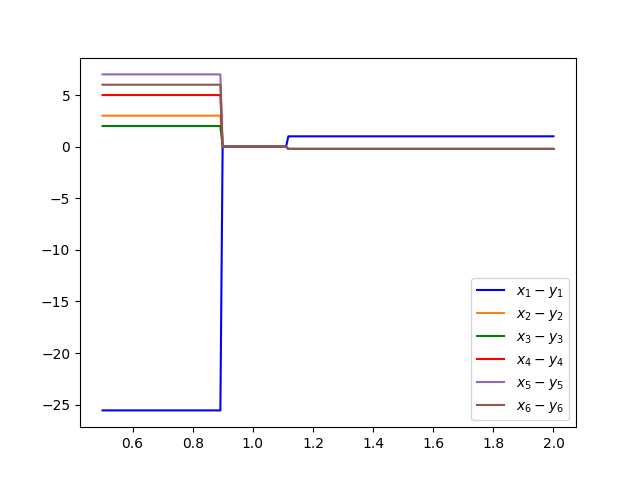
(a) Optimal trades $x-y$ for $t\in[0.5,2]$.

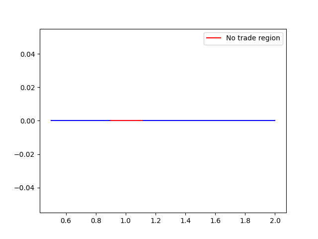
(b) No-trade region.

Figure 1: Market function $\varphi_{\mathrm{am}}$. One parameter case.

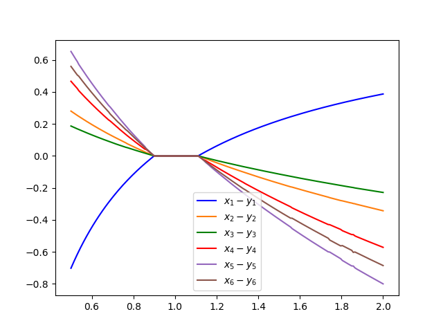
(a) Optimal trades $x-y$ for $t\in[0.5,2]$.

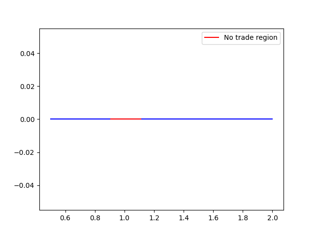
(b) No-trade region.

Figure 2: Market function $\varphi_{\mathrm{gm}}$. One parameter case.

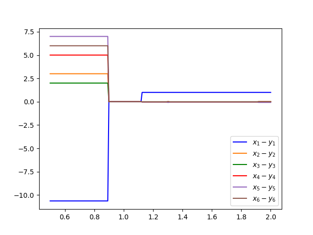
(a) Optimal trades $x-y$ for $t\in[0.5,2]$.

(b) No-trade region.

Figure 3: Market function $\varphi_{\mathrm{qm}}$. One parameter case.

Figure 4: Market function $\varphi_{\mathrm{qm}}$. Two parameter case.

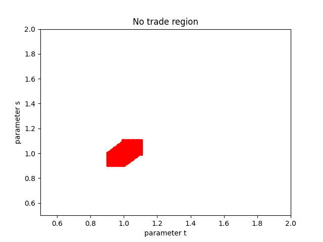
Figure 5: Market function $\varphi_{\mathrm{gm}}$. Two parameter case.

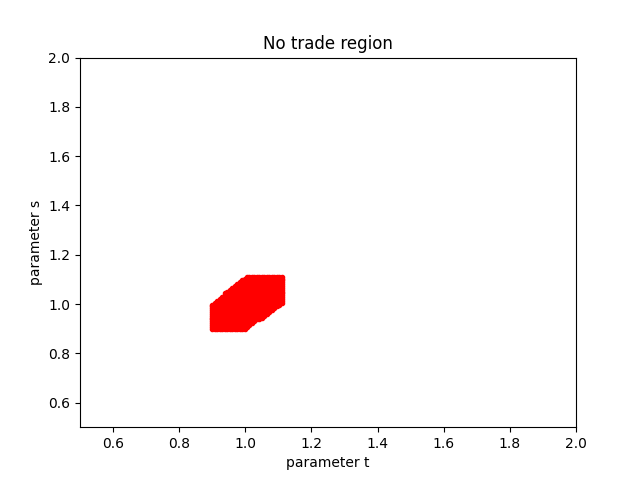
Figure 6: Market function $\varphi_{\mathrm{am}}$. Two parameter case.

5.3 Extensions

Many other examples are still possible. For instance, consider the (unweighted) quasi-arithmetic mean

$$\varphi:\mathbb{R}^{n}_{+} \longrightarrow \mathbb{R}$$

$$x=(x_{1},\cdots,x_{n}) \longmapsto f^{(-1)}\left[\frac{1}{n}\sum_{i=1}^{n}f(x_{i})\right],$$

which is of course a particular case of (5.1) (obtained by setting $\omega_{i}=1/n$ for $i=1,\cdots,n$). The function $f$ is still assumed to be continuous and strictly monotonic, so the mean is well-defined. If we further assume that $f\in C^{2}$ and $f^{\prime}\neq 0$, then the convexity of the mean is characterized in Theorem 3.1 of [32] and concavity is characterized in Theorem 2.2 of [31]. From now on we also assume that $f^{\prime}>0$, so the mean is strictly increasing and covered by the statement of Corollary 5.1. Since these characterizations require less regularity than those exposed in subsection 5.1, but the generators still fulfil the hypotheses of Corollary 5.1 (what means the means are quasi-linear), they open the possibility of constructing new trading functions included in our theory but not considered in [3]. Actually, even the weighted case (5.1), which was considered for $\mathcal{C}^{4}$ functions in [22] (see subsection 5.1), can be extended to $C^{2}$ functions (Theorem 5, [13]). Moreover, Theorem 1 of [13] asserts the essential equivalence between the weighted and the unweighted cases in relation to convexity/concavity. Finally, let us mention that this reference, [13], presents some explicit examples of generators that give rise to means that are neither convex nor concave and enjoy different degrees of smoothness. Consequently, they can be used as starting point to construct trading functions regarded by our theory but not that of [3]. One such mean, based on the smooth generator of Example 4 in [13], is given by the explicit formula:

$$\varphi(x)=\sum_{i=1}^{n}\left[\omega_{i}(x_{i}+e^{x_{i}})\right]-W_{0}\left\{\exp\left[\sum_{i=1}^{n}\omega_{i}(x_{i}+e^{x_{i}})\right]\right\}.$$ (5.3)

Extending the collection of examples is not just a matter of regularity. For instance, in [37], the family of generalized quasi-arithmetic means

$$\Phi:\mathbb{R}_{+}^{n} \longrightarrow \mathbb{R}$$

$$x=(x_{1},\cdots,x_{n}) \longmapsto F^{(-1)}\left[\sum_{i=1}^{n}\omega_{i}f_{i}(x_{i})\right],$$

is considered. In this case, the functions $f_{i}:\mathbb{R}_{+}\longrightarrow\mathbb{R}$ are $C^{2}$ and convex for all $i=1,\cdots,n$ (but no monotonicity assumption is in principle imposed). On the other hand, $F:\mathbb{R}_{+}\longrightarrow\mathbb{R}$ is required to be convex, strictly increasing, and $C^{2}$. This constitutes an obvious extension of the quasi-arithmetic means discussed in subsection 5.1. The convexity of these generalized quasi-arithmetic means is characterized in Theorem 2.2 in [37]. Moreover, one can characterize their concavity just by reverting the inequality in the statement of this theorem; the proof would follow identically mutatis mutandis. As these means constitute a structural generalization of the quasi-arithmetic means, they could also be used to build new trading functions falling under our more general umbrella, but not necessarily that of [3]. In such a case, one would need to consider the functions $f_{i}$ to be strictly increasing as well, in order to assure the quasi-linearity of $\Phi$ (since it would become the composition of two strictly increasing functions).

As a final note, we state the obvious fact that other generalizations of quasi-arithmetic means are indeed possible [10].

6 Conclusions

This paper has been devoted to the mathematical analysis of a sort of AMMs, the so called constant function market makers, which exchange algorithm is determined by a trade function. This function depends on the provision of the different liquidity pools and, keeping its constancy in every trade, sets the asset prices. The robustness of this type of AMMs against the attacks of arbitrageurs has been established in the literature under the assumption of a convex trade function [3]. These studies formulate the problem as a mathematical optimization and give conditions on the optimality of no trading whatsoever, what implies the absence of arbitrage, see [3] and references therein.

Herein, we have extended these previous works in several directions, but always restricted to those cases in which the trading functions are monotonically increasing, a usual assumption in the literature (which is also a characteristic property of means). First, we have considered the case of quasilinear, but not necessarily convex, trade functions. Then, we have not only characterized the no-trade region, but actually any type of optimal trade, and the former came as a consequence of the latter. We have also considered asset-dependent fees, rather than the uniform fee assumed in [3]. And finally, this all has served us to embed the construction of new possible trade functions into the theory of generalized means, which is well-studied from the mathematical viewpoint.

Our mathematical results aim to generalize the class of trade functions that can be used to construct the exchange algorithm over which an AMM is designed. In this spirit, we have given families of examples of constant function markets makers built based on trade functions that are quasilinear but not convex. Since popular AMMs such as Uniswap [2] and Balancer [27] use a trade function that is a mean (be it weighted or unweighted), we have constructed our quasilinear-but-not-convex trade functions as generalized means. The mathematical theory of generalized means is both rich and classical, what has facilitated their analysis as trade functions. Furthermore, we have performed the numerical optimization of AMM trading for three particular cases of trade functions: the arithmetic and geometric means (both with a well-defined convexity), and another exotic mean that is quasilinear but neither concave nor convex; therefore, the former are covered by the classical theory in [3], but not the latter, which is only regarded in our extension. Our numerical experiments show that all the three means behave similarly as trade functions. Therefore, quasilinear trade functions could in principle be as robust to arbitrage as convex/concave functions.

Overall, our results open the possibility of constructing new AMMs based on constant functions that are not necessarily either convex or concave, but still keep the robustness of the AMM against arbitrage attacks. Our preliminary numerical experiments suggest that some exotic means that are quasilinear but not convex (and not concave either) might serve to this purpose. Of course, more research is needed in order to check other properties of the so-generated AMMs. Clearly, we have to pay a price for the mathematical sophistication that the use of generalized means implies; but, at least in our opinion, this very same fact may carry about advantages too. In general terms, we believe that this line of research, which relies on the mathematical formalization of the AMM functioning and its systematic analysis, can serve to improve the design of constant function market makers; remarkably, it opens the possibility of doing so without the financial risk that related empirical studies might imply.

References

• [1] J. Aczél, On mean values, Bull. Amer. Math. Soc., 54, 392–400, (1948).
• [2] H. Adams, N. Zinsmeister, M. Salem, R. Keefer, D. Robinson, Uniswap v3 core. Technical Report, (2021).
• [3] G. Angeris, A. Agrawal, A. Evans, T. Chitra, and S. Boyd, Constant function market makers: multi-asset trades via convex optimization; in: D. A. Tran et al. (eds): “Handbook on Blockchain”. Springer Optimization and Its Applications, Vol. 194. Springer. (2022).
• [4] G. Angeris and T. Chitra, Improved price oracles: Constant function market makers; in Proceedings of the 2nd ACM Conference on Advances in Financial Technologies, ACM, New York. (2020).
• [5] G. Angeris, T. Chitra, and A. Evans, When Does The Tail Wag The Dog? Curvature and Market Making, Cryptoeconomic Systems, 2(1). https://doi.org/10.21428/58320208.e9e6b7ce. (2022).
• [6] G. Angeris, A. Evans, and T. Chitra, Replicating market makers, Digital Finance 5, 367–387, (2023).
• [7] G. Angeris, H.-T. Kao, R. Chiang, C. Noyes, and T. Chitra, An Analysis of Uniswap markets, Cryptoeconomic Systems, 0(1). https://doi.org/10.21428/58320208.c9738e64. (2021).
• [8] K.J. Arrow, A.C. Enthoven, Quasiconcave programming, Econometrica, 29, 779–800, (1961).
• [9] M. Avriel, W.E. Diewert, S. Schaible, I. Zang, Generalized Concavity. SIAM, Philadelphia, (2010).
• [10] M. Bajraktarević, Sur une équation fonctionnelle aux valeurs moyennes, Glasnik Mat.-Fiz. Astronom. Društvo Mat. Fiz. Hrvatske Ser. II, 13, 243–248, (1958).
• [11] N.G. de Bruijn, Asymptotic Methods in Analysis, North-Holland, Amsterdam, (1958).
• [12] A. Cambini, L. Martein. Generalized Convexity and Optimization. Springer-Verlag, Berlin-Heidelberg, (2009).
• [13] J. Chudziak, D. Głazowska, J. Jarczyk, W. Jarczyk, On weighted quasi-arithmetic means which are convex, Math. Inequal. Appl., 22, 1123–1136, (2019).
• [14] R. M. Corless, G. H. Gonnet, D. E. G. Hare, D. J. Jeffrey, D. E. Knuth, On the Lambert $W$ function, Adv. Comp. Math., 5, 329–359, (1996).
• [15] G. Debreu, Theory of value. John Wiley, New York, (1959).
• [16] M. Egorov, StableSwap – efficient mechanism for Stablecoin liquidity, (2019).
• [17] M. Ehrgott. Multicriteria optimization. Vol. 491, Springer Science $\&$ Business Media, (2005).
• [18] L. Euler, De serie Lambertina plurimisque eius insignibus proprietatibus, Acta Acad. Scient. Petropol. 2, 29–51, (1783).
• [19] B. de Finetti, Sul concetto di media, Giornale dell’ Instituto Italiano degli Attuarii 2, 369–396, (1931).
• [20] F.N. Fritsch, R.E. Shafer, W.P. Crowley, Algorithm 443: Solution of the transcendental equation $we^{w}=x$, Communications of the ACM 16, 123–124, (1973).
• [21] R. Hanson, Logarithmic markets coring rules for modular combinatorial information aggregation, The Journal of Prediction Markets. 1 (1), 3–15, (2012).
• [22] G. Hardy, J.L. Littlewood, G. Pólya, Inequalities, Cambridge University Press, London, (1934).
• [23] J. Jahn. Introduction to the theory of nonlinear optimization. Springer Nature, (2020).
• [24] K. Knopp, Über Reihen mit positiven Gliedern, J. London Math. Soc. 3, 205–211, (1928).
• [25] A.N. Kolmogorov, Sur la notion de la moyenne, Rend. Accad. dei Lincei 12, 388–391, (1930).
• [26] O.L. Mangasarian, Pseudo-convex functions, J. SIAM Control, Ser. A, 3, 281–290, (1965).
• [27] F. Martinelli, N. Mushegian, A non-custodial portfolio mannager, liquidity provider, and price sensor, (2019).
• [28] A. Mas-Colell, M.D. Whinston, J.R. Green, Microeconomic Theory. Oxford University Press, Oxford, (1995).
• [29] M. Nagumo, Über eine Klasse der Mittel werte, Japanese J. Math. 7, 71–79, (1930).
• [30] S. Nakamoto, Bitcoin: A peer-to-peer electronic cash system, https://bitcoin.org/bitcoin.pdf, (2008).
• [31] Z. Páles, P. Pasteczka, On the best Hardy constant for quasi-arithmetic means and homogeneous deviation means, Math. Inequal. Appl. 21, 585–599, (2018).
• [32] Z. Páles, P. Pasteczka, On the Jensen convex and Jensen concave envelopes of means, Archiv der Mathematik 116, 423–432, (2021).
• [33] G. Pólya, G. Szegö, Aufgaben und Lehrsätze der Analysis, Springer, Berlin, (1925).
• [34] S. Schaible, W.T. Ziemba. Generalized Concavity in Optimization and Economics. Academic Press. (1981).
• [35] P. Virtanen, et al. SciPy 1.0: Fundamental Algorithms for Scientific Computing in Python. Nature Methods, 17 (13) , 261-272, (2020).
• [36] E.M. Wright, Solution of the equation $ze^{z}=a$, Bull. Amer. Math. Soc. 65, 89–93, (1959).
• [37] Y.-B. Zhao, S.-C. Fang, D. Li, Constructing generalized mean functions using convex functions with regularity conditions, SIAM J. Optim. 17, 37–51, (2006).