Deep MMD Gradient Flow without adversarial training

Abstract

We propose a gradient flow procedure for generative modeling by transporting particles from an initial source distribution to a target distribution, where the gradient field on the particles is given by a noise-adaptive Wasserstein Gradient of the Maximum Mean Discrepancy (MMD). The noise-adaptive MMD is trained on data distributions corrupted by increasing levels of noise, obtained via a forward diffusion process, as commonly used in denoising diffusion probabilistic models. The result is a generalization of MMD Gradient Flow, which we call Diffusion-MMD-Gradient Flow or $\mathrm{DMMD}$. The divergence training procedure is related to discriminator training in Generative Adversarial Networks (GAN), but does not require adversarial training. We obtain competitive empirical performance in unconditional image generation on CIFAR10, MNIST, CELEB-A (64 x64) and LSUN Church (64 x 64). Furthermore, we demonstrate the validity of the approach when MMD is replaced by a lower bound on the KL divergence.

1 Introduction

In recent years, generative models have achieved impressive capabilities on image (Saharia et al., 2022), audio (Le et al., 2023) and video generation (Ho et al., 2022) tasks but also protein modeling (Watson et al., 2022) and 3d generation (Poole et al., 2022). Diffusion models (Sohl-Dickstein et al., 2015; Ho et al., 2020; Song et al., 2020; Rombach et al., 2022) underpin these new methods. In these models, we learn a backward denoising diffusion process via denoising score matching (Hyvärinen, 2005; Vincent, 2011). This backward process corresponds to the time-reversal of a forward noising process. At sampling time, starting from random Gaussian noise, diffusion models produce samples by discretizing the backward process.

One challenge that arises when applying these models in practice is that the Stein score (that is, the gradient log of the current noisy density) becomes ill-behaved near the data distribution (Yang et al., 2023): the diffusion process needs to be slowed down at this point, which incurs a large number of sampling steps near the data distribution. Indeed, if the manifold hypothesis holds (Tenenbaum et al., 2000; Fefferman et al., 2016; Brown et al., 2022) and the data is supported on a lower dimensional space, it is expected that the score will explode for noise levels close to zero, to ensure that the backward process concentrates on this lower dimensional manifold (Bortoli, 2023; Pidstrigach, 2022; Chen et al., 2022). While strategies exist to mitigate these issues, they trade-off the quality of the output against inference speed, see for instance (Song et al., 2023; Xu et al., 2023; Sauer et al., 2023).

Generative Adversarial Networks (GANs) (Goodfellow et al., 2014) represent an alternative popular generative modelling framework (Brock et al., 2019; Karras et al., 2020a). Candidate samples are produced by a generator: a neural net mapping low dimensional noise to high dimensional images. The generator is trained in alternation with a discriminator, which is a measure of discrepancy between the generator and target images. An advantage of GANs is that image generation is fast once the GAN is trained (Xiao et al., 2022), although image samples are of lower quality than for the best diffusion models (Ho et al., 2020; Rombach et al., 2022). When learning a GAN model, the main challenge arises due to the presence of the generator, which must be trained adversarially alongside the discriminator. This requires careful hyperparameter tuning (Brock et al., 2019; Karras et al., 2020b; Liu et al., 2020), without which GANs may suffer from training instability and mode collapse  (Arora et al., 2017; Kodali et al., 2017; Salimans et al., 2016).

Nonetheless, the process of GAN design has given rise to a strong understanding of discriminator functions, and a wide variety of different divergence measures have been applied. These fall broadly into two categories: the integral probability metrics (among which, the Wasserstein distance (Arjovsky et al., 2017; Gulrajani et al., 2017; Genevay et al., 2018) and the Maximum Mean Discrepancy (Li et al., 2017; Bińkowski et al., 2021; Arbel et al., 2018)) and the f-divergences (Goodfellow et al., 2014; Nowozin et al., 2016; Mescheder et al., 2018; Brock et al., 2019). While it would appear that f-divergences ought to suffer from the same shortcomings as diffusions when the target distribution is supported on a submanifold (Arjovsky et al., 2017), the divergences used in GANs are in practice variational lower bounds on their corresponding f-divergences (Nowozin et al., 2016), and in fact behave closer to IPMs in that they do not require overlapping support of the target and generator samples, and can metrize weak convergence (Arbel et al., 2021, Proposition 14) and (Zhang et al., 2018) (there remain important differences, however: notably, f-divergences and their variational lower bounds need not be symmetric in their arguments).

A natural question then arises: is it possible to define a Wasserstein gradient flow (Ambrosio et al., 2008; Santambrogio, 2015) using a GAN discriminator as a divergence measure? In this setting, the divergence (discriminator) provides a gradient field directly onto a set of particles (rather than to a generator), transporting them to the target distribution. Contributions in this direction include the MMD flow (Arbel et al., 2019; Hertrich et al., 2023), which defines a Wasserstein Gradient Flow on the Maximum Mean Discrepancy (Gretton et al., 2012); and the KALE (KL approximate lower-bound estimator) flow (Glaser et al., 2021), which defines a Wasserstein gradient flow on a KL lower bound of the kind used as a GAN discriminator based on an f-divergence (Nowozin et al., 2016). We describe the MMD and its corresponding Wasserstein gradient flow in Section 2. These approaches employ fixed function classes (namely, reproducing kernel Hilbert spaces) for the divergence, and are thus not suited to high dimensional settings such as images. Moreover, we show in this work that even for simple examples in low dimensions, an adaptive discriminator ensures faster convergence of a source distribution to the target, see Section 3.

A number of more recent approaches employ trained neural net features in divergences for a subsequent gradient flow (e.g. Fan et al., 2022; Franceschi et al., 2023). Broadly speaking, these works used adversarial means to train a series of discriminator functions, which are then applied in sequence to a population of particles. While more successful on images than kernel divergences, the approaches retain two shortcomings: they still require adversarial training (on their own prior output), with all the challenges that this entails; and their empirical performance falls short in comparison with modern diffusions and GANs (see related work in Section 7 for details).

In the present work, we propose a novel Wasserstein Gradient flow on a noise-adaptive MMD divergence measure, leveraging insights from both GANs and diffusion models. To train the discriminator, we start with clean data, and use a forward diffusion process from (Ho et al., 2020) to produce noisy versions of the data with given levels of noise (data with high levels of noise are analogous to the output of a poorly trained generator, whereas low noise is analogous to a well trained generator). The added noise is always Gaussian. For a given level of noise, we train a noise conditional MMD discriminator to distinguish between the clean and the noisy data, using a single network across all noise levels. This allows us to have better control over the discriminator training procedure than would be achievable with a GAN generator at different levels of refinement, where this control is implicit and hard to characterize.

To draw new samples, we propose a novel noise-adaptive version of MMD gradient flow (Arbel et al., 2019). We start from samples drawn from a Gaussian distribution, and move them in the direction of the target distribution by following MMD Gradient flow (Arbel et al., 2019), adapting our MMD discriminator to the corresponding level of noise. Details may be found in Section 4. This allows us to have a fine grained control over the sampling process. As a final challenge, MMD gradient flows have previously required large populations of interacting particles for the generation of novel samples, which is expensive (quadratic in the number of particles) and impractical. In Section 5, we propose a scalable approximate sampling procedure for a case of a linear base kernel, which allows single samples to be generated with a very little loss in quality, at cost idependent of the number of particles used in training. The MMD is an instance of an integral probability metric, however many GANs have been designed using discriminators derived from f-divergences. Section 6 demonstrates how our approach can equally be applied to such divergences, using a lower bound on the KL divergence as an illustration. Section 7 contains a review of alternative approaches to using GAN discriminators for sample generation. Finally, in Section 8, we show that our method, Diffusion-MMD-gradient flow ($\mathrm{DMMD}$), yields competitive performance in generative modeling on simple 2-D datasets as well as in unconditional image generation on CIFAR10 (Krizhevsky et al., 2009), MNIST, CELEB-A (64 x64) and LSUN Church (64 x 64).

2 Background

In this section, we define the MMD as a GAN discriminator, then describe Wasserstein gradient flow as it applies for this divergence measure.

MMD GAN.

Let $\mathcal{X}\subset\mathbb{R}^{D}$ and $\mathcal{P}(\mathcal{X})$ be the set of probability distributions defined on $\mathcal{X}$. Let $P\in\mathcal{P}(\mathcal{X})$ be the target or data distribution and $Q_{\psi}\in\mathcal{P}(\mathcal{X})$ be a distribution associated with a generator parameterized by $\psi\in\mathbb{R}^{L}$. Let $\mathcal{H}$ be Reproducing Kernel Hilbert Space (RKHS), see (Schölkopf & Smola, 2018) for details, for some kernel $k:\mathcal{X}\times\mathcal{X}\rightarrow\mathbb{R}$. The Maximum Mean Discrepancy (MMD) (Gretton et al., 2012) between $Q_{\psi}$ and $P$ is defined as $\mathrm{MMD}(Q_{\psi},P)=\sup_{\|f\|_{\mathcal{H}}\leq 1}\{\mathbb{E}_{Q_{\psi}}[f(X)]-\mathbb{E}_{P}[f(X)]\}$. We refer to the function $f_{Q_{\psi},P}$ that attains the supremum as the witness function,

$$\textstyle f_{Q_{\psi},P}(z)\propto\int k(x,z)\mathrm{d}Q_{\psi}(x)-\int k(y,z)\mathrm{d}P(y),$$ (1)

which will be essential in defining our gradient flow. Given $X^{N}=\{x_{i}\}_{i=1}^{N}\sim Q_{\psi}^{\otimes N}$ and $Y^{M}=\{y_{i}\}_{i=1}^{M}\sim P^{\otimes M}$, the empirical witness function is known in closed form,

$$\textstyle\hat{f}_{Q_{\psi},P}(x)\propto\tfrac{1}{N}\sum_{i=1}^{N}k(x_{i},x)-\tfrac{1}{M}\sum_{j=1}^{M}k(y_{j},x),$$ (2)

and an unbiased estimate of $\mathrm{MMD}^{2}$ (Gretton et al., 2012) is likewise straightforward. In the MMD GAN (Bińkowski et al., 2021; Li et al., 2017), the kernel is written

$$\textstyle k(x,y)=k_{\text{base}}(\phi(x;\theta),\phi(y;\theta)),$$ (3)

where $k_{\text{base}}$ is a base kernel and $\phi(\cdot;\theta):\mathcal{X}\rightarrow\mathbb{R}^{K}$ are neural networks discriminator features with parameters $\theta\in\mathbb{R}^{H}$. We use the modified notation $\mathrm{MMD}^{2}_{u}[X^{N},Y^{M};\theta]$ to highlight the functional dependence on the discriminator parameters. The $\mathrm{MMD}$ is an Integral Probability Metric (IPM) (Muller, 1997), and thus well defined on distributions with disjoint support: this argument was made in favor of IPMs by Arjovsky et al. (2017). Note further that the Wasserstein GAN discriminators of Arjovsky et al. (2017); Gulrajani et al. (2017) can be understood in the MMD framework, when the base kernel is linear. Indeed, it was observed by Genevay et al. (2018) that requiring closer approximation to a true Wasserstein distance resulted in decreased performance in GAN image generation, likely due to the the exponential dependence of sample complexity on dimension for the exact computation of the Wasserstein distance; this motivates an interpretation of these discriminators simply as IPMs using a class of linear functions of learned features. We further note that the variational lower bounds used in approximating f-divergences for GANs share the property of being well defined on distribtions with disjoint support (Nowozin et al., 2016; Arbel et al., 2021), although they need not be symmetric in their arguments. Finally, while $Q_{\psi}$ and $\theta$ are trained adversarially in GANs, our setting will only require us to learn the discriminator parameter $\theta$.

Wasserstein gradient flows.

An alternative to using a GAN generator is to instead move a sample of particles along the Wasserstein Gradient flow associated with the discriminator (Ambrosio et al., 2008). Let $\mathcal{P}_{2}(\mathcal{X})$ be a set of probability distributions on $\mathcal{X}$ with a finite second moment equipped with the 2-Wasserstein distance. Let $\mathcal{F}(\nu):\mathcal{P}_{2}(\mathcal{X})\rightarrow\mathbb{R}$ be a functional defined over $\mathcal{P}_{2}(\mathcal{X})$ with a property that $\arg\inf_{\nu}\mathcal{F}(\nu)=P$. We consider the problem of transporting mass from an initial distribution $\nu_{0}=Q$ to a target distribution $\mu=P$, by finding a continuous path $(\nu_{t})_{t\geq 0}$ starting from $\nu_{0}$ that converges to $\mu$. This problem is studied in Optimal Transport theory (Villani, 2008; Santambrogio, 2015). This path can be discretized as a sequence of random variables $(X_{n})_{n\in\mathbb{N}}$ such that $X_{n}\sim\nu_{n}$, described by

$$X_{n+1}=X_{n}-\gamma\nabla\mathcal{F}^{\prime}(\nu_{n})(X_{n}),\quad X_{0}\sim Q,$$ (4)

where $\eta>0$ and $\mathcal{F}^{\prime}(\nu_{n})(X_{n})$ is the first variation of $\mathcal{F}$ associated with the Wasserstein gradient, see (Ambrosio et al., 2008; Arbel et al., 2019) for precise definitions. As $n\rightarrow\infty$ and $\gamma\rightarrow 0$, depending on the conditions on $\mathcal{F}$, the process  (4) will convergence to the gradient flow as a continuous time limit (Ambrosio et al., 2008).

MMD gradient flow.

For a choice $\mathcal{F}(\nu)=\mathrm{MMD}^{2}[\nu,P]$ and a fixed kernel, conditions for convergence of the process in (4) to $P$ are given by Arbel et al. (2019). Moreover, the first variation of $\mathcal{F}^{\prime}(\nu)=f_{\nu,P}\in\mathcal{H}$ is the witness function defined earlier. Using (1)-(4), the discretized MMD gradient flow for any $n\in\mathbb{N}$ is given by

$$X_{n+1}=X_{n}-\gamma\nabla f_{\nu_{n},P}(X_{n}),\qquad X_{0}\sim Q.$$ (5)

This provides an algorithm to (approximately) sample from the target distribution $P$. We remark that Arbel et al. (2019); Hertrich et al. (2023) used a kernel with fixed hyperparameters. In the next section, we will argue that even for RBF kernels (where only the bandwidth is chosen), faster convergence will be attained using kernels that adapt during the gradient flow. Details of kernel choice for alternative approaches are given in related work (Section 7).

3 A motivation for adaptive kernels

In this section, we demonstrate the benefit of using an adaptive kernel when performing MMD gradient flow. We show that even in the simple setting of Gaussian sources and targets, an adaptive kernel improves the convergence of the flow. Consider the following normalized Gaussian kernel,

$$k_{\alpha}(x,y)=\alpha^{-d}\exp[-\|x-y\|^{2}/(2\alpha^{2})].$$ (6)

For any $\mu\in\mathbb{R}^{d}$ and $\sigma>0$ we denote by $\pi_{\mu,\sigma}$ the Gaussian distribution with mean $\mu$ and covariance matrix $\sigma^{2}\mathrm{Id}$. We denote $\mathrm{MMD}_{\alpha}$ the $\mathrm{MMD}$ associated with $k_{\alpha}$.

Proposition 3.1.

For any $\mu_{0}\in\mathbb{R}^{d}$ and $\sigma>0$, let $\alpha^{\star}$ be given by

$$\textstyle\alpha^{\star}=\mathrm{argmax}_{\alpha\geq 0}\|\nabla_{\mu_{0}}\mathrm{MMD}^{2}_{\alpha}(\pi_{0,\sigma},\pi_{\mu_{0},\sigma})\|.$$ (7)

Then, we have that

$$\alpha^{\star}=\mathrm{ReLU}(\|\mu_{0}\|^{2}/(d+2)-2\sigma^{2})^{1/2}.$$ (8)

The result is proved in Appendix F. The quantity $\|\nabla_{\mu_{0}}\mathrm{MMD}^{2}_{\alpha}(\pi_{0,\sigma},\pi_{\mu_{0},\sigma})\|$ represents how much the mean of the Gaussian $\pi_{\mu_{0},\sigma}$ is displaced by a flow w.r.t. $\mathrm{MMD}^{2}_{\alpha}$. Intuitively, we want $\|\nabla_{\mu_{0}}\mathrm{MMD}^{2}_{\alpha}(\pi_{0,\sigma},\pi_{\mu_{0},\sigma})\|$ to be as large as possible as this represents the maximum displacement possible.

We show that $\alpha^{\star}$ maximizing this displacement is given by (8). It is notable that assuming that when $\sigma>0$ is fixed, this quantity depends on $\|\mu_{0}\|$, i.e. the distance between the two distributions. This observation justifies our approach of following an adaptive MMD flow at inference time. We further highlight the phase transition behaviour of Proposition 3.1: once the Gaussians are sufficiently close, the optimal kernel width is zero (note that this phase transition would not be observed in the simpler Dirac GAN example of Mescheder et al. (2018), where the source and target distributions are Dirac masses with no variance). This phase transition suggests that the flow associated with $\mathrm{MMD}$ benefits less from adaptivity as the supports of the distributions overlap. We exploit this observation by introducing an optional denoising stage to our procedure; see the end of Section 4.

In practice, it is not desirable to approximate the distributions of interest by Gaussians, and richer neural network kernel features $\phi(x;\theta)$ are used (see Section 8). Approaches to optimize the MMD parameters for GAN training are described by Arbel et al. (2018), which serve as proxies for convergence speed: notably, it is not sufficient simply to maximize the MMD, since the witness function should remain Lipschitz to ensure convergence (Arbel et al., 2018, Proposition 2). This is achieved in practice by controlling the gradient of the witness function; we take a similar approach in Section 4.

4 Diffusion Maximum Mean Discrepancy Gradient Flow

In this section, we present Diffusion Maximum Mean Discrepancy gradient flow ($\mathrm{DMMD}$), a new generative model with a training procedure of $\mathrm{MMD}$ discriminator which does not rely on adversarial training, and leverages ideas from diffusion models. The sampling part of $\mathrm{DMMD}$ consists in following a noise adaptive variant of $\mathrm{MMD}$ gradient flow.

4.1 Adversarial-free training of noise conditional discriminators

In order to train a discriminator without adversarial training, we propose to use insights from GANs training. In a GAN setting, at the beginning of the training, the generator is randomly initialized and therefore produces samples close to random noise. This would produce a coarse discriminator since it is trained to distinguish clean data from random noise. As the training progresses and the generator improves so does the discriminative power of the discriminator. This behavior of the discriminator is central in the training of GANs (Goodfellow et al., 2014). We propose a way to replicate this gradually improving behavior without adversarial training and instead relying on principles from diffusion models (Ho et al., 2020).

The forward process in diffusion models allows us to generate a probability path $P_{t},t\in[0,1]$, such that $P_{0}=P$, where $P$ is our target distribution and $P_{1}=\mathrm{N}(0,\mathrm{Id})$ is a Gaussian noise. Given samples $x_{0}\sim P_{0}=P$, the samples $x_{t}|x_{0}$ are given by

$$x_{t}=\alpha_{t}x_{0}+\beta_{t}\epsilon,\quad\epsilon\in\mathrm{N}(0,\mathrm{Id}),$$ (9)

with $\alpha_{0}=\beta_{1}=1$ and $\alpha_{1}=\beta_{0}=0$. From (9), we observe that for low noise level $t$, the samples $x_{t}$ are very close to the original data $x_{0}$, whereas for the large values of $x_{t}$ they are close to a unit Gaussian random variable. Using the GANs terminology, $x_{t}$ could be thought as the output of a generator such that for high/low noise level $t$, it would correspond to undertrained / well-trained generator.

Using this insight, for each noise level $t\in[0,1]$, we define a discriminator $\mathrm{MMD}^{2}(P_{t},P;t,\theta)$ using the kernel of type (3) with noise-conditional discriminator features $\phi(x;t;\theta)$ parameterized by a Neural Network with learned parameters $\theta$. We consider the following noise-conditional loss function

$$\mathcal{L}(\theta,t)=-\mathrm{MMD}^{2}(P_{t},P;t,\theta)$$ (10)

where the minus sign comes from the fact that our aim is to maximize the squared MMD. In addition, we regularize this loss with $\ell_{2}$-penalty (Bińkowski et al., 2021) denoted $\mathcal{L}_{\ell_{2}}(\theta,t)$ as well as with the gradient penalty (Bińkowski et al., 2021; Gulrajani et al., 2017) denoted $\mathcal{L}_{\nabla}(\theta,t)$, see Appendix B.2 for the precise definition of these two losses. The total noise-conditional loss is then given as

$$\mathcal{L}_{\text{tot}}(\theta,t)=\mathcal{L}(\theta,t)+\lambda_{\ell_{2}}\mathcal{L}_{\ell_{2}}(\theta,t)+\lambda_{\nabla}\mathcal{L}_{\nabla}(\theta,t),$$ (11)

for a suitable choice of hyperparameters $\lambda_{\ell_{2}}\geq 0,\lambda_{\nabla}\geq 0$. Finally, the total loss is given as

$$\mathcal{L}_{\text{tot}}(\theta)=\mathbb{E}_{t\sim U[0,1]}\left[\mathcal{L}_{\text{tot}}(\theta,t)\right],$$ (12)

where $U[0,1]$ is a uniform distribution on $[0,1]$. In practice, we use sampled-based unbiased estimator of MMD, see Appendix B.2. The procedure is described in Algorithm 1.

Algorithm 1 Train noise-conditional $\mathrm{MMD}$ discriminator

  Input: Dataset $\mathcal{D}=\{x_{i}\}_{i=1}^{N}$

  Discriminator features $\phi(x,t;\theta)$ with parameters $\theta\in\mathbb{R}^{K}$

  $\lambda_{\nabla}\geq 0,\lambda_{\ell_{2}}\geq 0$ - gradient and $\ell_{2}$ penalty coefficients

  $\gamma>0$ is the learning rate

  $N_{\text{iter}}$ is the number of iterations, $B$ is a batch size

  $N_{\text{noise}}$ is the number of noise levels per batch

  for $i=1$ to $N_{\text{iter}}$ do

     Sample a batch $B$ of clean data $X_{0}\sim P(X_{0})$

     for $n=1$ to $N_{\text{noise}}$ do

        Sample noise level $t_{n}\sim U[0,1]$

        Sample $X_{t_{n}}\sim p(X_{t_{n}}|X_{0},t_{n})$ using eqn. (9)

        Let $\phi^{X_{0}}_{t_{n}}=\phi(X_{0},t_{n};\theta)$, $\phi^{X_{t_{n}}}_{t_{n}}=\phi(X_{t_{n}},t_{n};\theta)$

        For linear kernel, compute $\mathrm{MMD}$ loss (10) using (42)

        Compute the loss $\mathcal{L}_{\text{tot}}(\theta,t_{n})$ using eqn. (11)

     end for

     Compute total loss $\mathcal{L}_{\text{tot}}(\theta)=\frac{1}{N_{\text{noise}}}\sum_{n=1}^{N_{\text{noise}}}\mathcal{L}_{\text{tot}}(\theta,t_{n})$

     Update discriminator features

     $\theta\leftarrow\mathrm{ADAM}(\theta,\mathcal{L}_{\text{tot}}(\theta),\gamma)$

  end for

4.2 Adaptive gradient flow sampling

In order to produce samples from $P$, we use the adaptive $\mathrm{MMD}$ gradient flow with noise conditional discriminators $\mathrm{MMD}^{2}[P_{t},P;t;\theta^{\star}]$, where $\theta^{\star}$ are the discriminator parameters obtained using Algorithm 1. Let $t_{i}=t_{\text{min}}+i\Delta t,i=0,\ldots,T$ be the noise discretisation, where $\Delta t=(t_{\text{max}}-t_{\text{min}})/T$ such that $t_{0}=t_{\text{min}},t_{T}=t_{\text{max}}$ for some $t_{\text{min}}=\epsilon$ and $t_{\text{max}}=1-\epsilon$, where $\epsilon<\!\!\!<1$. We sample $N_{\text{p}}$ initial particles $\{Z^{i}|Z^{i}\sim\mathrm{N}(0,\mathrm{Id})\}_{i=1}^{N_{\text{p}}}$. For each $t$, we follow MMD gradient flow (5) for $N_{\text{s}}$ steps with learning rate $\eta>0$

$$\textstyle Z^{i,n+1}_{t}=Z^{i,n}_{t}-\eta\nabla f_{\nu_{N_{\text{p}},n}^{t},P}(Z^{i,n}_{t},t;\theta^{\star}).$$ (13)

Here $\nu_{N_{\text{p}},n}^{t}=1/N_{\text{p}}\sum_{i=1}^{N_{\text{p}}}\updelta_{Z^{t}_{i,n}}$ is the empirical distribution of particles $\{Z^{i,n}_{t}\}_{i=1}^{N_{\text{p}}}$ at the noise level $t$ and the iteration $n$, $\updelta$ is a Dirac mass measure. The function $f_{\nu_{N_{\text{p}},n}^{t},P}(z,t;\theta^{\star})$ is adapted from equation (1) where $\nu$ is replaced by this empirical distribution. After following the gradient flow (13) for $N_{\text{s}}$ steps, we initialize a new gradient flow with initial particles $Z_{t-\Delta t}^{i,0}=Z^{i,N_{\text{s}}}_{t}$ for each $i=1,\ldots,N_{\text{p}}$, with the decreased level of noise $t-\Delta t$. The recurrence is initialized with $Z_{t_{\text{max}}}^{i,0}=Z^{i}$ where $\{Z^{i}\}_{i=1}^{N_{\text{p}}}$ are the initial particles. This procedure corresponds to running $T+1$ consecutive MMD gradient flows for $N_{\text{s}}$ iterations each, gradually decreasing the noise level $t$ from $t_{\text{max}}$ to $t_{\text{min}}$. The resulting particles $\{Z_{t_{\text{min}}}^{i,N_{\text{s}}}\}_{i=1}^{N_{\text{p}}}$ are then used as samples from $P$. The procedure is described in Algorithm 2.

In practice, we sample (once) a large batch $N_{c}$ of $\{X^{j}_{0}\}_{j=1}^{N_{c}}\sim P^{\otimes N_{c}}$ from the data distribution and denote by $\hat{P}_{N_{\text{c}}}(X_{0})$ the corresponding empirical distribution. Then we use the empirical witness function (2) given by

$$f_{\nu_{N_{\text{p}},n}^{t},\hat{P}_{N_{\text{c}}}(X_{0})}(z,t;\theta^{\star})=$$ (14)

$$\quad\textstyle\frac{1}{N_{\text{p}}}\sum_{i=1}^{N_{\text{p}}}k_{\text{base}}(\phi(Z^{n,i}_{t},t;\theta^{\star}),\phi(z,t;\theta^{\star}))$$ (15)

$$\qquad\textstyle-\frac{1}{N_{\text{c}}}\sum_{j=1}^{N_{\text{c}}}k_{\text{base}}(\phi(X^{j}_{0},t;\theta^{\star}),\phi(z,t;\theta^{\star})).$$ (16)

Final denoising.

In diffusion models (Ho et al., 2020), it is common to use a denoising step at the end to improve samples quality. Empirically, we found that doing a few $\mathrm{MMD}$ gradient flow steps at the end of the sampling with a higher learning rate $\eta$ allowed to reduce the amount of noise and improve performance.

Algorithm 2 Noise-adaptive $\mathrm{MMD}$ gradient flow

  Inputs: $T$ is the number of noise levels

  $t_{\text{max}},t_{\text{min}}$ are maximum and minimum noise levels

  $N_{\text{s}}$ is the number of gradient flow steps per noise level

  $\eta>0$ is the gradient flow learning rate

  $N_{\text{p}}$ is the number of noisy particles

  Batch of clean particles $X_{0}\sim\mathcal{P}_{0}$.

  Steps: Sample initial noisy particles $Z\sim\mathrm{N}(0,\mathrm{Id})$

  Set $\Delta t=(t_{\text{max}}-t_{\text{min}})/T$

  for $i=T$ to $0$ do

     Set the noise level $t=t_{\text{min}}+i\Delta t$ and $Z^{0}_{t}=Z$

     for $n=0$ to $N_{\text{s}}-1$ do

        Compute $f_{\nu_{N_{\text{p}},n}^{t},\hat{P}_{N_{\text{c}}}(X_{0})}(Z^{n}_{t},t;\theta^{\star})$ using (16)

        $Z^{n+1}_{t}=Z^{n}_{t}-\eta\nabla f_{\nu_{N_{\text{p}},n}^{t},\hat{P}_{N_{\text{c}}}(X_{0})}(Z^{n}_{t},t;\theta^{\star})$

     end for

     Set $Z=Z^{N}_{t}$

  end for

  Output $Z$

5 Scalable $\mathrm{DMMD}$ with linear kernel

The computation complexity of the $\mathrm{MMD}$ estimate on two sets of $N$ samples is $O(N^{2})$, so as of the witness function (16) for $N$ noisy and clean particles. This makes scaling to large $N$ prohibitive. Using linear base kernel (see (3))

$$\textstyle k_{\text{base}}(x,y)=\langle x,y\rangle,$$ (17)

allows to reduce the computation complexity of both quantities down to $O(N)$, see Appendix B.3. We consider the average noise conditional discriminator features on the whole dataset

$$\textstyle\bar{\phi}(X_{0},t;\theta^{\star})=\frac{1}{N}\sum_{i=1}^{N}\phi(X^{i}_{0},t;\theta^{\star}).$$ (18)

Using linear kernel (17) allows us to use these average features (18) in the second term of (16). In practice, we can precompute these features for $T$ timesteps and store them in memory in order to use them for sampling purposes. The associated storage cost is $O(TK)$ where $K$ is the dimensionality of these features.

Approximate sampling procedure.

$\mathrm{MMD}$ gradient flow (13) requires us to use multiple interacting particles $Z$ to produce samples, where the interaction is captured by the first term in (16). In practice this means that the performance will depend on the number of these particles. In this section, we propose an approximation to $\mathrm{MMD}$ gradient flow with a linear base kernel (17) which allows us to sample particles independently, therefore removing the need for multiple particles. For a linear kernel, the interaction term in (16) for a particle $Z$, equals to

$$\textstyle\langle\frac{1}{N_{\text{p}}}\sum_{i=1}^{N_{\text{p}}}\phi(Z^{n,i}_{t},t;\theta^{\star}),\phi(Z,t;\theta^{\star})\rangle,$$ (19)

For a large number of particles $N_{\text{p}}$, the contribution of each particle $Z^{t}_{n,i}$ on the interaction term with $Z$ will be small. For a sufficiently large $N_{\text{p}}$, we hypothesize that

$$\textstyle\frac{1}{N_{\text{p}}}\sum_{i=1}^{N_{\text{p}}}\phi(Z^{n,i}_{t},t;\theta^{\star})\approx\frac{1}{N}\sum_{j=1}^{N}\phi(X^{j}_{t},t;\theta^{\star}),$$ (20)

where $N$ is the size of the dataset and $X^{j}_{t}$ are produced by the forward diffusion process (9) applied to each $X^{j}_{0}$. In Section 8, we test this approximation in practice.

Using (20), we consider an approximate witness function

$$\textstyle\hat{f}_{P_{t},P}(z)=\langle\phi(z,t;\theta^{*}),\bar{\phi}(X_{t},t;\theta^{\star})-\bar{\phi}(X_{0},t;\theta^{\star})\rangle,$$ (21)

with $\bar{\phi}(X_{t},t;\theta^{\star})$ precomputed using (18). In practice, we sample single particle $Z\sim\mathrm{N}(0,\mathrm{Id})$ and follow noise-adaptive $\mathrm{MMD}$ gradient flow with (21)

$$\textstyle Z^{n+1}_{t}=Z^{n}_{t}-\eta\nabla\hat{f}_{P_{t},P}(Z^{n}_{t})$$ (22)

The corresponding algorithm is described in Appendix B.4.

6 f-divergences

The approach described in Section 4 can be applied to any divergence which has a well defined Wasserstein Gradient Flow described by a gradient of the associated witness function. Such divergences include the variational lower bounds on f-divergences, as described by (Nowozin et al., 2016), which are popular in GAN training, and were indeed the basis of the original GAN discriminator (Goodfellow et al., 2014). One such f-divergence is the KL Approximate Lower bound Estimator (KALE, Glaser et al., 2021). Unlike the original KL divergence, which requires a density ratio, the KALE remains well defined for distributions with non-overlapping support. Similarly to $\mathrm{MMD}$, the Wasserstein Gradient of $\mathrm{KALE}$ is given by the gradient of a learned witness function. Therefore, we train noise-conditional $\mathrm{KALE}$ discriminator and use corresponding noise-conditional Wasserstein gradient flow, similarly to $\mathrm{DMMD}$. We call this method Diffusion $\mathrm{KALE}$ flow ($\mathrm{D}$-$\mathrm{KALE}$-Flow). The full approach is described in Appendix D. We found this approach to lead to reasonable empirical results, but unlike with $\mathrm{DMMD}$, it achieved worse performance than a corresponding GAN, see Appendix E.4.

7 Related Work

Adversarial training and $\mathrm{MMD}$-GAN.

Integral Probability Metrics (IPMs) are good candidates to define discriminators in the context of generative modeling, since they are well defined even in the case of distributions with non-overlapping support (Muller, 1997). Moreover, implementations of f-divergence discriminators in GANs rely on variational lower bounds (Nowozin et al., 2016): as noted earlier, these share useful properties of IPMs in theory and in practice (notably, they remain well defined for distributions with disjoint support, and may metrize weak convergence for sufficiently rich witness function classes (Arbel et al., 2021, Proposition 14) and (Zhang et al., 2018)). Several works (Arjovsky et al., 2017; Gulrajani et al., 2017; Genevay et al., 2018; Li et al., 2017; Bińkowski et al., 2021) have exploited IPMs as discriminators for the training of GANs, where the IPMs are MMDs using (linear or nonlinear) kernels defined on learned neural net features, making them suited to high dimensional settings such as image generation. Interpreting the IPM-based GAN discriminator as a squared $\mathrm{MMD}$ yields an interesting theoretical insight: Franceschi et al. (2022) show that training a GAN with an IPM objective implicitly optimizes $\mathrm{MMD}^{2}$ in the Neural Tangent Kernel (NTK) limit (Jacot et al., 2020). IPM GAN discriminators are trained jointly with the generator in a min-max game. Adversarial training is challenging, and can suffer from instability, mode collapse, and misconvergence (Xiao et al., 2022; Bińkowski et al., 2021; Li et al., 2017; Arora et al., 2017; Kodali et al., 2017; Salimans et al., 2016). Note that once a GAN has been trained, the samples can be refined via MCMC sampling in the generator latent space (e.g., using kinetic Langevin dynamics; see Ansari et al., 2021; Che et al., 2021; Arbel et al., 2021).

Discriminator flows for generative modeling.

Wasserstein Gradient flows (Ambrosio et al., 2008; Santambrogio, 2015) applied to a GAN discriminator are informally called discriminator flows, see (Franceschi et al., 2023). A number of recent works have focused on replacing a GAN generator by a discriminator flow. Fan et al. (2022) propose a discretisation of JKO (Jordan et al., 1998) scheme to define a Kullback-Leibler (KL) divergence gradient flow. Other approaches have used a discretized interactive particle-based approach instead of JKO, similar to (4). Heng et al. (2023); Franceschi et al. (2023) build such a flow based on f-divergences, whereas Franceschi et al. (2023) focuses on $\mathrm{MMD}$ gradient flow. In all these works, an explicit generator is replaced by a corresponding discriminator flow. The sampling process during training is as follows: Let $Y_{k}$ be the samples produced at training iteration $k$ by the gradient flow $\mathcal{F}_{k}$ induced by the discriminator $\mathcal{D}_{k}$ applied to samples $Y_{k-1}$ from the previous iteration. We denote this by $Y_{k}\leftarrow\mathcal{F}_{k}(\mathcal{D}_{k},Y_{k-1})$. Then, the discriminator at iteration $k+1$ is trained on samples $Y_{k}$. A challenge of this process is that the training sample for the next discriminator will be determined by the previous discriminators, and thus the generation process is still adversarial: particle transport minimizes the previous discriminator value, and the subsequent discriminator is maximized on these particles. Consequently, it is difficult to control or predict the overall sample trajectory from the initial distribution to the target, which might explain the performance shortfall of these methods in image generation settings. By contrast, we have explicit control over the training particle trajectory via the forward noising diffusion process.

On top of that, these approaches (except for Heng et al., 2023) require to store all intermediate discriminators $\mathcal{D}_{1},\ldots,\mathcal{D}_{N}$ throughout training ($N$ is the total number of training iterations). These discriminators are then used to produce new samples by applying the sequence of gradient flows $\mathcal{F}_{N}(\mathcal{D}_{N},\cdot)\circ\ldots\circ\mathcal{F}_{1}(\mathcal{D}_{1},\cdot)$ to $Y_{0}$ sampled from the initial distribution. This creates a large memory overhead.

An alternative is to use pretrained features obtained elsewhere or a fixed kernel with empirically selected hyperparameters (see Hertrich et al., 2023; Hagemann et al., 2023; Altekrüger et al., 2023) , however this limits the applicability of the method. To the best of our knowledge, our approach is the first to demonstrate the possibility to train a discriminator without adversarial training, such that this discriminator can then be used to produce samples with a gradient flow. Unlike the alternatives, our approach does not require to store intermediate discriminators.

$\mathrm{MMD}$ for diffusion refinement/regularization.

$\mathrm{MMD}$ has been used to either regularize training of diffusion models (Li & van der Schaar, 2024) or to finetune them (Aiello et al., 2023) for fast sampling. The $\mathrm{MMD}$ kernel in these works has the form (3) with Inception features (Szegedy et al., 2014). Our method removes the need to use pretrained features by training th $\mathrm{MMD}$ discriminator.

Diffusion models.

Diffusion models (Sohl-Dickstein et al., 2015; Ho et al., 2020; Song et al., 2020) represent a powerful new family of generative models due to their strong empirical performance in many domains (Saharia et al., 2022; Le et al., 2023; Ho et al., 2022; Watson et al., 2022; Poole et al., 2022). Unlike GANs, diffusion models do not require adversarial training. At training time, a denoiser is learned for multiple noise levels. As noted above, our work borrows from the training of diffusion models, as we train a discriminator on multiple noise levels of the forward diffusion process (Ho et al., 2020). This gives better control of the training samples for the (noise adapted) discriminator than using an incompletely trained GAN generator.

8 Experiments

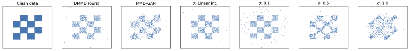
Figure 1: Samples from $\mathrm{MMD}$ Gradient flow with different parameters for the RBF kernel (23).

8.1 Understanding $\mathrm{DMMD}$ behavior in 2-D

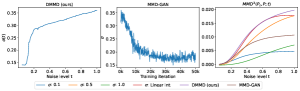
Figure 2: Qualitative behaviour of $\mathrm{MMD}$ discriminators. Left, learned RBF kernel (23) widths $\sigma(t)$ as a function of noise level $t$. Center, parameter $\sigma$ for $\mathrm{MMD}$-GAN as function of training iteration. Right, $\mathrm{MMD}^{2}(P_{t},P;t)$ for different methods.

The aim of the experiments in this section is to get an understanding of the behavior of $\mathrm{DMMD}$ described in Section 4. We expect $\mathrm{DMMD}$ to mimic GAN discriminator training via noise conditional discriminator learning. To see whether this manifests in practice, we design a toy experiment using Radial Basis Function (RBF) kernel for $\mathrm{MMD}$

$$k_{t}(x,y)=\exp[-\|x-y\|^{2}/(2\sigma^{2}(t;\theta))],$$ (23)

where the noise dependent kernel width function $\sigma(\cdot;\theta):[0,1]\rightarrow[0,+\infty)$ is parameterized by $\theta\in\mathbb{R}^{K}$. This parameter controls the coarseness of the $\mathrm{MMD}$ discriminator.

We consider a simple checkerboard 2-D dataset, see Figure 1, left. We learn noise-conditional kernel widths $\sigma(t;\theta)$ using a neural network ensuring that $\sigma(t;\theta)>0$. As baselines, we consider $\mathrm{MMD}$-GAN with a trained generator and a discriminator with one learnable parameter $\sigma$. On top of that, we consider $\mathrm{MMD}$ gradient flow with fixed values of $\sigma$ and a variant called linear interpolation with manually chosen noise-dependent $\sigma(t)=0.1(1-t)+0.5t$. All experimental details are provided in Appendix C.

We report the learned RBF kernel widths for $\mathrm{DMMD}$ in Figure 2, left. As expected, as noise level goes from high to low, the kernel width $\sigma(t)$ decreases. In Figure 2, center, we show the learned $\mathrm{MMD}$-GAN kernel width parameter $\sigma$ as a function of training iterations. As expected, when the training progresses, this parameter decreases, since the corresponding generator produces samples, close to the target distribution. The behaviors of $\mathrm{DMMD}$ and $\mathrm{MMD}$-GAN are quite similar. Interestingly, the range of values for the kernel widths is also similar. This highlights our point that $\mathrm{DMMD}$ mimics the training of a GAN discriminator. The exact dynamics for $\sigma(t)$ in $\mathrm{DMMD}$ depends on the parameters of the forward diffusion process (9). The sharp phase transition is consistent with the phase transition highlighted in Section 3. In addition, we report $\mathrm{MMD}^{2}(P_{t},P;t)$ for different methods in Figure 2, right. We observe that the behavior of $\mathrm{DMMD}$ is close to linear interpolation variant, but is more nuanced for higher noise levels. Finally, we report the corresponding samples in Figure 1. We see that $\mathrm{DMMD}$ produces visually better samples than the other baselines. For RBF kernel, we noticed the presence of outliers. The amount of outliers generally depends on the kernel, see Appendix of (Hertrich et al., 2023) for more details.

8.2 Image generation

We study the performance of $\mathrm{DMMD}$ on unconditional image generation of CIFAR10 (Krizhevsky et al., 2009). We use the same forward diffusion process as in (Ho et al., 2020) to produce noisy images. We use a U-Net (Ronneberger et al., 2015) backbone for discriminator feature network $\phi(x,t;\theta)$, with a slightly different architecture from the one used in (Ho et al., 2020), see Appendix E. For all the image-based experiments, we use linear base kernel (17). We explored using other kernels such as RBF and Rational Quadratic (RQ), but did not find an improvement in performance. We use FID (Heusel et al., 2018) and Inception Score (Salimans et al., 2016) for evaluation, see Appendix E. Unless specified otherwise, we use the number $N_{\text{p}}=200$ of particles for Algorithm 2. We provide ablation over the number of particles in Appenidx E.3. The total number of iterations for $\mathrm{DMMD}$ equals to $T\times N_{\text{s}}$, where $T$ is the number of noise levels and $N_{\text{s}}$ is the number of steps per noise level. To be consistent with diffusion models, we call this number number of function evaluations (NFE). For $\mathrm{DMMD}$, we report performance with different NFEs.

As baselines we consider our implementation of $\mathrm{MMD}$-GAN (Bińkowski et al., 2021) with linear base kernel and DDPM (Ho et al., 2020) using the same neural network backbones as for $\mathrm{DMMD}$. We also report results from the original papers. On top of that, we consider baselines based on discriminator flows. JKO-Flow (Fan et al., 2022), which uses JKO (Jordan et al., 1998) scheme for the KL gradient flow. Deep Generative Wasserstein Gradient Flows (DGGF-KL) (Heng et al., 2023), which uses particle-based approach (similar to (4)) for the KL gradient flow. These approaches use adversarial training to train discriminators, see Section 7 for more details. On top of that, we consider Generative Sliced $\mathrm{MMD}$ Flows with Riesz Kernels (GS-$\mathrm{MMD}$-RK) (Hertrich et al., 2023) which uses similar particle based approach to DGGF-KL to construct $\mathrm{MMD}$ flow, but uses fixed (kernel) discriminator. On top of that, we report results using a discriminator flow defined on a trained $\mathrm{MMD}$-GAN discriminator which we call $\mathrm{MMD}$-GAN-Flow. More details on experiments are given in Appendix E. The results are provided in Table 1.

Table 1: Unconditional image generation on CIFAR-10. For $\mathrm{MMD}$ GAN (orig.), we used mixed-RQ kernel described in (Bińkowski et al., 2021). ”Orig.” stands for the original paper and ”impl.” stands for our implementation. For JKO-Flow (Fan et al., 2022), the NFE is taken from their Figure 12.

Method	FID	Inception Score	NFE
MMD GAN (orig.)	39.90	6.51	-
MMD GAN (impl.)	13.62	8.93	-
DDPM (orig.)	3.17	9.46	1000
DDPM (impl.)	5.19	8.90	100
Discriminator flow baselines
DGGF-KL	28.80	-	110
JKO-Flow	23.10	7.48	$\sim 150$
MMD flow baselines
MMD-GAN-Flow	450	1.21	100
GS-MMD-RK	55.00	-	86
DMMD (ours)	8.31	9.09	100
DMMD (ours)	7.74	9.12	250

We see that $\mathrm{DMMD}$ achieves better performance than the $\mathrm{MMD}$ GAN. As expected, $\mathrm{MMD}$-GAN-Flow does not work at all. This is because the $\mathrm{MMD}$-GAN discriminator at convergence was trained on samples close to the target distribution. Making a parallel with RBF kernel experiment from Section 8.1, this means that the gradient of $\mathrm{MMD}$ will be very small on samples far away from the target distribution. This highlights the benefit of adaptive $\mathrm{MMD}$ discriminators. Moreover, we also see that $\mathrm{DMMD}$ performs better than GS-MMD-RK, which uses fixed kernel. This highlights the advantage of learning discriminator features in $\mathrm{DMMD}$. We see that $\mathrm{DMMD}$ achieves superior performance compared to other discriminator flow baselines. We believe that one of the reasons why these methods perform worse than $\mathrm{DMMD}$ consists in the need to use the adversarial training, which makes the hyperparameters choice tricky. $\mathrm{DMMD}$ on the other hand, relies on a simple non-adversarial training procedure from Algortihm 1. Finally, we see that DDPM performs better than $\mathrm{DMMD}$. This is not surprising, since both, U-Net architecture and forward diffusion process (9) were optimized for DDPM performance. Nevertheless, $\mathrm{DMMD}$ demonstrates strong empirical performance as a discriminator flow method trained without adversarial training. The samples from our method are provided in Appendix G.1.

Approximate sampling.

We run approximate $\mathrm{MMD}$ gradient flow (22) with the same discriminator as for $\mathrm{DMMD}$. We call this variant $a$-$\mathrm{DMMD}$, where $a$ stands for approximate. On top of that, we use denoising procedure described in Section 4.2. Starting from the samples given by $a$-$\mathrm{DMMD}$, we do $2$ gradient flow steps with higher learning rate using either approximate gradient flow (22), which we call $a$-$\mathrm{DMMD}$-$a$, or exact gradient flow (13) applied to a single particle, which we call $a$-$\mathrm{DMMD}$-$e$, $e$ stands for exact. On top of that, we apply the denoising to $\mathrm{DMMD}$, which we call $\mathrm{DMMD}$-$e$. Results are provided in Table 4. We observe that $a$-$\mathrm{DMMD}$ performs worse than $\mathrm{DMMD}$, which is as expected. Applying a denoising step improves performance of $a$-$\mathrm{DMMD}$, bringing it closer to $\mathrm{DMMD}$. This suggests that the approximation (20) moves the particles close to the target distribution; but once close to the target, a more refined procedure is required. By contrast, we see that denoising helps $\mathrm{DMMD}$ only marginally. This suggests that the exact noise-conditional witness function (16) accurately captures fine detais close to the target distribution.

Table 2: Approximate sampling performance on CIFAR10.

Method	FID	Inception Score	NFE
$\mathrm{DMMD}$	8.31	9.09	100
$\mathrm{DMMD}$-$e$	8.21	8.99	102
$a$-$\mathrm{DMMD}$	24.86	9.10	50
$a$-$\mathrm{DMMD}$-$e$	9.185	8.70	52
$a$-$\mathrm{DMMD}$-$a$	11.22	9.00	52

8.3 Results on CELEB-A, LSUN-Church and MNIST

Besides CIFAR-10, we study the performance of $\mathrm{DMMD}$ on MNIST (Lecun et al., 1998), CELEB-A (64x64 (Liu et al., 2015) and LSUN-Church (64x64) (Yu et al., 2016). For MNIST and CELEB-A, we consider the same splits and evaluation regime as in (Franceschi et al., 2023). For LSUN Church, the splits and the evaluation regime are taken from (Ho et al., 2020). For more details, see Appendix E.1. The results are provided in Table 3. In addition to $\mathrm{DMMD}$, we report the performance of Discriminator flow baseline from (Franceschi et al., 2023) with numbers taken from the corresponding paper. We see that $\mathrm{DMMD}$ performance is significantly better compared to the discriminator flow, which is consistent with our findings on CIFAR-10. The corresponding samples are provided in Appendix G.2.

Table 3: Unconditional image generation on additional datasets. The metric used is FID. The number of gradient flow steps for $\mathrm{DMMD}$ is 100.

Dataset	$\mathrm{DMMD}$	Disc. flow (Franceschi et al., 2023)
MNIST	3.0	4.0
CELEB-A	8.3	41.0
LSUN	6.1	-

9 Conclusion

In this paper we have presented a method to train a noise conditional discriminator without adversarial training, using a forward diffusion process. We use this noise conditional discriminator to generate samples using a noise adaptive MMD gradient flow. We provide theoretical insight into why an adaptive gradient flow can provide faster convergence than the non-adaptive variant. We demonstrate strong empirical performance of our method on uncoditional image generation of CIFAR10, as well as on additional, similar image datasets. We propose a scalable approximation of our approach which has close to the original empirical performance.

A number of questions remain open for future work. The empirical performance of $\mathrm{DMMD}$ will be of interest in regimes where diffusion models could be ill-behaved, such as in generative modeling on Riemannian manifolds; as well as on larger datasets such as ImageNet. $\mathrm{DMMD}$ provides a way of training a discriminator, which may be applicable in other areas where a domain-adaptive discriminator might be required. Finally, it will be of interest to establish theoretical foundations for $\mathrm{DMMD}$ in general settings, and to derive convergence results for the associated flow.

10 Impact statement

In recent years, generative modeling has undergone a period of rapid and transformative progress. Diffusion models play a pivotal role in driving this revolution with applications ranging from image synthesis to protein modeling. Recent works have sought ways to combined the strengths of both GANs and diffusion models. In this spirit, we propose in this work a new methodology for generative modeling, demonstrating that noise-adaptive discriminators may be defined to produce such flows without adversarial training. We believe that our work can shed light on the key components of these successful generative models and pave the way for further improvements of discriminative flow methods.

Appendix A Organization of the supplementary material

In Section B, we describe in details the training and sampling procedures for $\mathrm{DMMD}$. In Section C, we describe more details for the 2d experiments. In Section D, we provide more details about $\mathrm{DKALE}$-Flow method. In Section E, we provide experimental details for the image datasets. In Section F, we provide proof for the theoretical results described in Section 3 from the main section of the paper. Finally, in Section G we present the samples from $\mathrm{DMMD}$ on different image datasets.

Appendix B $\mathrm{DMMD}$ training and sampling

B.1 MMD discriminator

Let $\mathcal{X}\subset\mathbb{R}^{D}$ and $\mathcal{P}(\mathcal{X})$ be the set of probability distributions defined on $\mathcal{X}$. Let $P\in\mathcal{P}(\mathcal{X})$ be the target or data distribution and $Q_{\psi}\in\mathcal{P}(\mathcal{X})$ be a distribution associated with a generator parameterized by $\psi\in\mathbb{R}^{L}$. Let $\mathcal{H}$ be Reproducing Kernel Hilbert Space (RKHS), see (Schölkopf & Smola, 2018) for details, for some kernel $k:\mathcal{X}\times\mathcal{X}\rightarrow\mathbb{R}$. Maximum Mean Discrepancy (MMD) (Gretton et al., 2012) between $Q_{\psi}$ and $P$ is defined as $\mathrm{MMD}(Q_{\psi},P)=\sup_{f\in\mathcal{H}}\{\mathbb{E}_{Q_{\psi}}[f(X)]-\mathbb{E}_{P}[f(X)]\}$. Given $X^{N}=\{x_{i}\}_{i=1}^{N}\sim Q_{\psi}^{\otimes N}$ and $Y^{M}=\{y_{i}\}_{i=1}^{M}\sim P^{\otimes M}$, an unbiased estimate of $\mathrm{MMD}^{2}$ (Gretton et al., 2012) is given by

$$\textstyle\mathrm{MMD}^{2}_{u}[X^{N},Y^{M}]=\tfrac{1}{N(N-1)}\sum_{i\neq j}^{N}k(x_{i},x_{j})+$$ (24)

$$\textstyle\tfrac{1}{M(M-1)}\sum_{i\neq j}^{M}k(y_{i},y_{j})-\tfrac{2}{NM}\sum_{i=1}^{N}\sum_{j=1}^{M}k(x_{i},y_{j}).$$

In MMD GAN (Bińkowski et al., 2021; Li et al., 2017), the kernel in the objective (24) is given as

$$\textstyle k(x,y)=k_{\text{base}}(\phi(x;\theta),\phi(y;\theta)),$$ (25)

where $k_{\text{base}}$ is a base kernel and $\phi(\cdot;\theta):\mathcal{X}\rightarrow\mathbb{R}^{K}$ are neural networks discriminator features with parameters $\theta\in\mathbb{R}^{H}$. We use the modified notation of $\mathrm{MMD}^{2}_{u}[X^{N},Y^{M};\theta]$ for equation (24) to highlight the functional dependence on the discriminator parameters. $\mathrm{MMD}$ is an instance of Integral Probability Metric (IPM) (see (Arjovsky et al., 2017)) which is well defined on distributions with disjoint support unlike f-divergences (Nowozin et al., 2016). An advantage of using MMD over other IPMs (see for example, Wasserstein GAN (Arjovsky et al., 2017)) is the flexibility to choose a kernel $k$. Another form of $\mathrm{MMD}$ is expressed as a norm of a witness function

$$\mathrm{MMD}(Q_{\psi},P)=\sup_{f\in\mathcal{H}}\{\mathbb{E}_{Q_{\psi}}[f(X)]-\mathbb{E}_{P}[f(X)]\}=\|f_{Q_{\psi},P}\|_{\mathcal{H}},$$ (26)

where the witness function $f_{Q_{\psi},P}$ is given as

$$f_{Q_{\psi},P}(z)=\int k(x,z)dQ_{\psi}-\int k(y,z)dP(y)$$ (27)

Given two sets of samples $X^{N}=\{x_{i}\}_{i=1}^{N}\sim Q_{\psi}^{\otimes N}$ and $Y^{M}=\{y_{i}\}_{i=1}^{M}\sim P^{\otimes M}$, and the kernel (25), the empirical witness function is given as

$$\hat{f}_{Q_{\psi},P}(z)=\frac{1}{N}\sum_{i=1}^{N}k_{\text{base}}(\phi(x_{i};\theta),\phi(z;\theta))-\frac{1}{M}\sum_{j=1}^{M}k_{\text{base}}(\phi(y_{j};\theta),\phi(z;\theta))$$ (28)

The $\ell_{2}$ penalty (Bińkowski et al., 2021) is defined as

$$\mathcal{L}_{\ell_{2}}(\theta)=\frac{1}{N}\sum_{i=1}^{N}\|\phi(x_{i};\theta)\|^{2}_{2}+\frac{1}{N}\sum_{i=1}^{N}\|\phi(y_{i};\theta)\|^{2}_{2}$$ (29)

Assuming that $M=N$ and following (Bińkowski et al., 2021; Gulrajani et al., 2017), for $\alpha_{i}\sim U[0,1]$, where $U[0,1]$ is a uniform distribution on $[0,1]$, we construct $z_{i}=x_{i}\alpha_{i}+(1-\alpha)y_{i}$ for all $i=1,\ldots,N$. Then, the gradient penalty (Bińkowski et al., 2021; Gulrajani et al., 2017) is defined as

$$\mathcal{L}_{\nabla}(\theta)=\frac{1}{N}\sum_{i=1}^{N}(\|\nabla\hat{f}_{Q_{\psi},P}(z_{i})\|_{2}-1)^{2}$$ (30)

We denote by $\mathcal{L}(\theta)$ the $\mathrm{MMD}$ discriminator loss given as

$$\mathcal{L}(\theta)=-\mathrm{MMD}^{2}_{u}[X^{N},Y^{M};\theta]=\tfrac{1}{N(N-1)}\sum_{i\neq j}^{N}k_{\text{base}}(\phi(x_{i};\theta),\phi(x_{j};\theta))+\tfrac{1}{M(M-1)}\sum_{i\neq j}^{M}k_{\text{base}}(\phi(y_{i};\theta),\phi(y_{j};\theta))$$ (31)

$$\textstyle-\tfrac{2}{NM}\sum_{i=1}^{N}\sum_{j=1}^{M}k_{\text{base}}(\phi(x_{i};\theta),\phi(y_{j};\theta))$$ (32)

Then, the total loss for the discriminator on the two samples of data assuming that $N=M$ is given as

$$\mathcal{L}_{\text{tot}}(\theta)=\mathcal{L}(\theta)+\lambda_{\nabla}\mathcal{L}_{\nabla}(\theta)+\lambda_{\ell_{2}}\mathcal{L}_{\ell_{2}}(\theta),$$ (33)

for some constants $\lambda_{\nabla}\geq 0$ and $\lambda_{\ell_{2}}\geq 0$.

B.2 Noise-dependent $\mathrm{MMD}$

In Section 4, we describe the approach to train $\mathrm{MMD}$ discriminator from forward diffusion using noise-dependent discriminators. For that, we assume that we are given a noise level $t\sim U[0,1]$ where $U[0,1]$ is a uniform distribution on $[0,1]$, and a set of clean data $X^{N}=\{x^{i}\}_{i=1}^{N}\sim P^{\otimes N}$. Then we produce a set of noisy samples $x^{i}_{t}$ using forward diffusion process (9). We denote these samples by $X^{N}_{t}=\{x^{i}_{t}\}_{i=1}^{N}$. We define noise conditional kernel

$$k(x,y;t,\theta)=k_{\text{base}}(\phi(x,t;\theta),\phi(y,t;\theta)),$$ (34)

with noise conditional features $\phi(x,t;\theta)$. This allows us to define the noise conditional discriminator loss

$$\mathcal{L}(\theta,t)=-\mathrm{MMD}^{2}_{u}[X^{N},X^{N}_{t},t,\theta]=\tfrac{1}{N(N-1)}\sum_{i\neq j}^{N}k_{\text{base}}(\phi(x^{i}_{t};t,\theta),\phi(x^{j}_{t};t,\theta))+\tfrac{1}{N(N-1)}\sum_{i\neq j}^{N}k_{\text{base}}(\phi(x^{i};t,\theta),\phi(x^{j};t,\theta))$$ (35)

$$\textstyle-\tfrac{2}{N^{2}}\sum_{i=1}^{N}\sum_{j=1}^{N}k_{\text{base}}(\phi(x^{i};t,\theta),\phi(x^{j}_{t};t,\theta))$$ (36)

The noise conditional $\ell_{2}$ penalty is given as

$$\mathcal{L}_{\ell_{2}}(\theta,t)=\frac{1}{N}\sum_{i=1}^{N}\|\phi(x^{i}_{t};t,\theta)\|^{2}_{2}+\frac{1}{N}\sum_{i=1}^{N}\|\phi(x^{i};t,\theta)\|^{2}_{2}$$ (37)

The noise conditional gradient penalty is given as

$$\mathcal{L}_{\nabla}(\theta,t)=\frac{1}{N}\sum_{i=1}^{N}(\|\nabla\hat{f}_{P,t}(z_{i})\|_{2}-1)^{2},$$ (38)

where $z_{i}=\alpha_{i}x^{i}_{t}+(1-\alpha_{i})x^{i}$ for $\alpha_{i}\sim U[0,1]$ and the noise conditional witness function

$$\hat{f}_{P,t}(z)=\frac{1}{N}\sum_{i=1}^{N}k_{\text{base}}(\phi(x^{t}_{i};t,\theta),\phi(z;\theta))-\frac{1}{N}\sum_{j=1}^{N}k_{\text{base}}(\phi(x_{i};t,\theta),\phi(z;\theta))$$ (39)

Therefore, the total noise conditional loss is given as

$$\mathcal{L}_{\text{tot}}(\theta,t)=\mathcal{L}(\theta,t)+\lambda_{\nabla}\mathcal{L}_{\nabla}(\theta,t)+\lambda_{\ell_{2}}\mathcal{L}_{\ell_{2}}(\theta,t),$$ (40)

for some constants $\lambda_{\nabla}\geq 0$ and $\lambda_{\ell_{2}}\geq 0$.

B.3 Linear kernel for scalable $\mathrm{MMD}$

Computational complexity of (40) is $O(N^{2})$. Here, we assume that the base kernel is linear, i.e.

$$k_{\text{base}}(x,y)=\langle x,y\rangle$$ (41)

This allows us to simplify the $\mathrm{MMD}$ computation (35) as

$$\mathrm{MMD}^{2}_{u}[X^{N},X^{N}_{t},t,\theta]=\frac{1}{N(N-1)}\left(\bar{\phi_{t}}(X^{N}_{t})^{T}\bar{\phi_{t}}(X^{N}_{t})-\bar{\|\phi_{t}\|^{2}}^{N}(X_{t})\right)+\frac{1}{N(N-1)}\left(\bar{\phi_{t}}(X^{N})^{T}\bar{\phi_{t}}(X^{N})-\bar{\|\phi_{t}\|^{2}}^{N}(Y)\right)\\ -\frac{2}{NN}(\bar{\phi_{t}}(X^{N}_{t}))^{T}\bar{\phi_{t}}(X^{N}),$$ (42)

where

$$\bar{\phi_{t}}(X^{N}_{t})=\sum_{i=1}^{N}\phi(x^{i}_{t};\theta_{t})$$ (43)

$$\bar{\phi_{t}}(X^{N})=\sum_{j=1}^{N}\phi(x^{i};\theta_{t})$$ (44)

$$\bar{\|\phi_{t}\|^{2}}(X^{N}_{t})=\sum_{i=1}^{N}\|\phi(x^{i}_{t};\theta_{t})\|^{2}$$ (45)

$$\bar{\|\phi_{t}\|^{2}}(X^{N})=\sum_{j=1}^{N}\|\phi(x^{i};\theta_{t})\|^{2}$$ (46)

Therefore we can pre-compute quantities $\bar{\phi_{t}}(X^{N}_{t}),\bar{\phi_{t}}(X^{N}),\bar{\|\phi_{t}\|^{2}}(X^{N}_{t}),\bar{\|\phi_{t}\|^{2}}(X^{N})$ which takes $O(N)$ and compute $\mathrm{MMD}^{2}_{u}[X^{N},X^{N}_{t},t,\theta]$ in $O(1)$ time. This also leads $O(1)$ computation complexity for $\mathcal{L}_{\ell_{2}}$ and $O(N)$ complexity for $\mathcal{L}_{\nabla}$. This means that we simplify the computational complexity to $O(N)$ from $O(N^{2})$.

At sampling, following (13) requires to compute the witness function (39) for each particle, which for a general kernel takes $O(N^{2})$ in total. Using the linear kernel above, simplifies the complexity of the witness as follows

$$\hat{f}_{P,t}(z)=\langle\bar{\phi_{t}}(Z^{N})-\bar{\phi_{t}}(X^{N}),\phi(z;\theta)\rangle,$$ (47)

where $Z^{N}$ is a set of $N$ noisy particles. We can precompute $\bar{\phi_{t}}(Z^{N})$ in $O(N)$ time. Therefore one iteration of a witness function will take $O(1)$ time and for $N$ noisy particles it makes $O(N)$.

B.4 Approximate sampling procedure

In this section we provide an algorithm for the approximate sampling procedure. The only change with the original Algorithm 2 is the approximate witness function

$$\hat{f}^{\star}_{P_{t},P}(z)=\langle\phi(z,t;\theta^{\star}),\bar{\phi}(X_{t},t,\theta^{\star})-\bar{\phi}(X_{0},t,\theta^{\star})\rangle,$$ (48)

where

$$\bar{\phi}(X_{0},t,\theta^{\star}=\frac{1}{N}\sum_{i=1}^{N}\phi(x^{i}_{0},t;\theta^{\star})$$ (49)

$$\bar{\phi}(X_{t},t,\theta^{\star}=\frac{1}{N}\sum_{i=1}^{N}\phi(x^{i}_{t},t;\theta^{\star})$$ (50)

Here $x^{i}_{0},i=1,\ldots,N$ correspond to the whole training set of clean samples and $x^{i}_{t},i=1,\ldots,$ correspond to the noisy version of these clean samples produced by the forward diffusion process 9 for a given noise level $t$. These features can be precomputed once for every noise level $t$. The resulting algorithm is given in Algorithm (3). Another crucial difference with the original algorithm is the ability to run it for each particle $Z$ independently.

Algorithm 3 Approximate noise-adaptive $\mathrm{MMD}$ gradient flow for a single particle

  Inputs: $T$ is the number of noise levels

  $t_{\text{max}},t_{\text{min}}$ are maximum and minimum noise levels

  $N_{\text{s}}$ is the number of gradient flow steps per noise level

  $\eta>0$ is the gradient flow learning rate

  $\bar{\phi}(X_{0},t,\theta^{\star})$ - precomputed clean features for all $t=1,\ldots,T$ with (49)

  $\bar{\phi}(X_{t},t,\theta^{\star})$ - precomputed noisy features for all $t=1,\ldots,T$ with (49)

  Steps: Sample initial noisy particle $Z\sim\mathrm{N}(0,\mathrm{Id})$

  for $i=T$ to $0$ do

     Set the noise level $t=i\Delta t$ and $Z^{t}_{0}=Z$

     for $n=0$ to $N_{\text{s}}-1$ do

        $Z^{t}_{n+1}=Z^{t}_{n}-\eta\langle\nabla_{z}\phi(Z^{t}_{n},t;\theta^{\star}),\bar{\phi}(X_{t},t,\theta^{\star})-\bar{\phi}(X_{0},t,\theta^{\star})\rangle$

     end for

     Set $Z=Z^{t}_{N}$

  end for

  Output $Z$

Appendix C Toy 2-D datasets experiments

For the 2-D experiments, we train $\mathrm{DMMD}$ using Algorithm (1) for $N_{\text{iter}}=50000$ steps with a batch size of $B=256$ and a number of noise levels per batch equal to $N_{\text{noise}}=128$. The Gradient penalty constant $\lambda_{\nabla}=0.1$ whereas the $\ell_{2}$ penalty is not used. To learn noise-conditional $\mathrm{MMD}$ for $\mathrm{DMMD}$, we use a $4$-layers MLP $g(t;\theta)$ with ReLU activation to encode $\sigma(t;\theta)=\sigma_{\text{min}}+\text{ReLU}(g(t;\theta))$ with $\sigma_{\text{min}}=0.001$, which ensures $\sigma(t;\theta)>0$. The MLP layers have the architecture of $[64,32,16,1]$. Before passing the noise level $t\in[0,1]$ to the MLP, we use sinusoidal embedding similar to the one used in (Ho et al., 2020), which produces a feature vector of size $1024$. The forward diffusion process from (Ho et al., 2020) have modified parameters such that corresponding $\beta_{1}=10^{-}4,\beta_{T}=0.0002$. On top of that, we discretize the corresponding process using only $1000$ possible noise levels, with $t_{\text{min}}=0.05$ and $t_{\text{max}}=1.0$. At sampling time for the algorithm 2, we use $t_{\text{min}}=0.05,t_{\text{max}}=1.0$, $N_{\text{s}}=10$ and $T=100$. The learning rate $\eta=1.0$. As basleines, we consider $\mathrm{MMD}$-GAN with a generator parameterised by a $3$-layer MLP with ELU activations. The architecture of the MLP is $[256,256,2]$. The initial noise for the generator is produced from a uniform distribution $U[-1,1]$ with a dimensionality of $128$. The gradient penalty coefficient equals to $0.1$. As for the discriminator, the only learnable parameter is $\sigma$. We train $\mathrm{MMD}$-GAN for $250000$ iterations with a batch size of $B=256$. Other variants of $\mathrm{MMD}$ gradient flow use the same sampling parameters as $\mathrm{DMMD}$.

Appendix D D-KALE-flow

In this section, we describe the $\mathrm{DKALE}$-flow algorithm mentioned in Section 6. Let $\mathcal{X}\subset\mathbb{R}^{D}$ and $\mathcal{P}(\mathcal{X})$ be the set of probability distributions defined on $\mathcal{X}$. Let $P\in\mathcal{P}(\mathcal{X})$ be the target or data distribution and $Q\in\mathcal{P}(\mathcal{X})$ be some distribution. The KALE objective (see (Glaser et al., 2021)) is defined as

$$KALE(Q,P|\lambda)=(1+\lambda)\max_{h\in\mathcal{H}}\{1+\int hdQ-\int e^{h}dP-\frac{\lambda}{2}||h||^{2}_{\mathcal{H}}\},$$ (51)

where $\lambda\geq 0$ is a positive constant and $\mathcal{H}$ is the RKHS with a kernel $k$. In practice, KALE divergence (51) can be replaced by a corresponding parametric objective

$$KALE(Q,P|\lambda,\theta,\alpha)=(1+\lambda)\left(\int h(X;\theta,\alpha)dQ(X)-\int e^{h(Y;\theta,\alpha)}dP(Y)-\frac{\lambda}{2}||\alpha||^{2}_{2}\right),$$ (52)

where

$$h(X;\theta,\alpha)=\phi(X;\theta)^{T}\alpha,$$ (53)

with $\phi(X;\theta)\in\mathbb{R}^{D}$ and $\alpha\in\mathbb{R}^{D}$. The objective function (52) can then be maximized with respect to $\theta$ and $\alpha$ for given $Q$ and $P$. Similar to $\mathrm{DMMD}$, we consider a noise-conditional witness function

$$h(x;t,\theta,\alpha,\psi)=\phi(x;t,\theta)^{T}\alpha({t};\psi)$$ (54)

From here, the noise-conditional KALE objective is given as

$$\mathcal{L}(\theta,\psi,t|\lambda)=KALE(P_{t},P|\lambda,\theta,\alpha),$$ (55)

where $P_{t}$ is the distribution corresponding to a forward diffusion process, see Section 4.1. Then, the total noise-conditional objective is given as

$$\mathcal{L}_{\text{tot}}(\theta,\psi,t|\lambda)=\mathcal{L}(\theta,\psi,t|\lambda)+\lambda_{\nabla}\mathcal{L}_{\nabla}(\theta,\psi,t)+\lambda_{\ell_{2}}\mathcal{L}_{\ell_{2}}(\theta,t),$$ (56)

where gradient penalty has similar form to WGAN-GP (Gulrajani et al., 2017)

$$\mathcal{L}_{\nabla}(\theta,\psi,t)=\mathbb{E}_{Z}(||\nabla_{Z}h(Z;t,\theta,\alpha,\psi)||_{2}-1)^{2},$$ (57)

where $Z=\beta X+(1-\beta)Y$, $\beta\sim U[0,1]$, $X\sim P(X)$ and $Y\sim P(Y)$. The l2 penalty is given as

$$\mathcal{L}_{\ell_{2}}(\theta,t)=\frac{1}{2}\left(\mathbb{E}_{X\sim P(X)}||\phi(X;t,\theta)||^{2}+\mathbb{E}_{Y\sim P(Y)}||\phi(Y;t,\theta)||^{2}\right)$$ (58)

Therefore, the final objective function to train the discriminator is

$$\mathcal{L}_{\text{tot}}(\theta,\psi|\lambda)=\mathbb{E}_{t\sim U[0,1]}\left[\mathcal{L}_{\text{tot}}(\theta,\psi,t|\lambda)\right]$$ (59)

This objective function depends on RKHS regularization $\lambda$, on gradient penalty regularization $\lambda_{\nabla}$ and on l2-penalty regularization $\lambda_{\ell_{2}}$. Unlike in $\mathrm{DMMD}$, we do not use an explicit form for the witness function and do not use the RKHS parameterisation. On one hand, this allows us to have a more scalable approach, since we can compute $\mathrm{KALE}$ and the witness function for each individual particle. On the other hand, the explicit form of the witness function in $\mathrm{DMMD}$ introduces beneficial inductive bias. In $\mathrm{DMMD}$, when we train the discriminator, we only learn the kernel features, i.e. corresponding RKHS. In $\mathrm{D}$-$\mathrm{KALE}$, we need to learn both, the kernel features $\phi(x;t,\theta)$ as well as the RKHS projections $\alpha(t;\psi)$. This makes the learning problem for $\mathrm{D}$-$\mathrm{KALE}$ more complex. The corresponding noise adaptive gradient flow for $\mathrm{KALE}$ divergence is described in Algorithm 4. An advantage over original $\mathrm{DMMD}$ gradient flow is the ability to run this flow individually for each particle.

Algorithm 4 Noise-adaptive $\mathrm{KALE}$ flow for single particle

  Inputs: $T$ is the number of noise levels

  $t_{\text{max}},t_{\text{min}}$ are maximum and minimum noise levels

  $N_{\text{s}}$ is the number of gradient flow steps per noise level

  $\eta>0$ is the gradient flow learning rate

  Trained witness function $h(\cdot;t,\theta^{\star},\psi^{\star})$

  Steps: Sample initial noisy particle $Z\sim\mathrm{N}(0,\mathrm{Id})$

  Set $\Delta t=(t_{\text{max}}-t_{\text{min}})/T$

  for $i=T$ to $0$ do

     Set the noise level $t=t_{\text{min}}+i\Delta t$ and $Z^{t}_{0}=Z$

     for $n=0$ to $N_{\text{s}}-1$ do

        $Z^{t}_{n+1}=Z^{t}_{n}-\eta\nabla h(Z^{t}_{n};t,\theta^{\star},\psi^{\star})$

     end for

     Set $Z=Z^{t}_{N}$

  end for

  Output $Z$

Appendix E Image generation experiments

For the image experiments, we use CIFAR10 (Krizhevsky et al., 2009) dataset. We use the same forward diffusion process as in (Ho et al., 2020). As a Neural Network backbone, we use U-Net (Ronneberger et al., 2015) with a slightly modified architecture from (Ho et al., 2020). Our neural network architecture follows the backbone used in (Ho et al., 2020). On top of that we output the intermediate features at four levels – before down sampling, after down-sampling, before upsampling and a final layer. Each of these feature vectors is processed by a group normalization, the activation function and a linear layer producing an output vector of size $32$. To produce the output of a discriminator features, these four feature vectors are concatenated to produce a final output feature vector of size $128$. The noise level time is processed via sinusoidal time embedding similar to (Ho et al., 2020). We use a dropout of $0.2$. $\mathrm{DMMD}$ is trained for $N_{\text{iter}}=250000$ iterations with a batch size $B=64$ with number $N_{\text{noise}}=16$ of noise levels per batch. We use a gradient penalty $\lambda_{\nabla}=1.0$ and $\ell_{2}$ regularisation strength $\lambda_{\ell_{2}}=0.1$. As evaluation metrics, we use FID (Heusel et al., 2018) and Inception Score (Salimans et al., 2016) using the same evaluation regime as in (Ho et al., 2020). To select hyperparameters and track performance during training, we use FID evaluated on a subset of $1024$ images from a training set of CIFAR10.

For CIFAR10, we use random flip data augmentation.

In $\mathrm{DMMD}$ we have two sets of hyperparameters, one is used for training in Algorithm 1 and one is used for sampling in Algorithm 2. During training, we fix the sampling parameters and always use these to select the best set of training time hyperparameters. We use $\eta=0.1$ gradient flow learning rate, $T=10$ number of noise levels, $N_{\text{p}}=200$ number of noisy particles, $N_{\text{s}}=5$ number of gradient flow steps per noise level, $t_{\text{min}}=0.001$ and $t_{\text{max}}=1-0.001$. We use a batch of $400$ clean particles during training. For hyperparameters, we do a grid search for $\lambda_{\nabla}\in\{0,0.001,0.01,0.1,1.0,10.0\}$, for $\lambda_{\ell_{2}}\in\{0,0.001,0.01,0.1,1.0,10.0\}$, for dropout rate $\{0,0.1,0.2,0.3\}$, for batch size $\{16,32,64\}$. To train the model, we use the same optimization procedure as in (Ho et al., 2020), notably Adam (Kingma & Ba, 2017) optimizer with a learning rate $0.0001$. We also swept over the the dimensionality of the output layer $32,64,128$, such that each of four feature vectors got the equal dimension. Moreover, we swept over the number of channels for U-Net $\{32,64,128\}$ (the original one was $32$) and we found that $128$ gave us the best empirical results.

After having selected the training-time hyperparameters and having trained the model, we run a sweep for the sampling time hyperparameters over $\eta\in\{1,0.5,0.1,0.04,0.01\}$, $T\in\{1,5,10,50\}$, $N_{\text{s}}\in\{1,5,10,50\}$, $t_{\text{min}}\in\{0.001,0.01,0.1,0.2\}$, $t_{\text{max}}\in\{0.9,1-0.001\}$. We found that the best hyperparameters for $\mathrm{DMMD}$ were $\eta=0.1$, $N_{\text{s}}=10$, $T=10$, $t_{\text{min}}=0.1$ and $t_{\text{max}}=0.9$. On top of that, we ran a variant for $\mathrm{DMMD}$ with $T=50$ and $N_{\text{s}}=5$.

For $a$-$\mathrm{DMMD}$ method, we used the same pretrained discriminator as for $\mathrm{DMMD}$ but we did an additional sweep over sampling time hyperparameters, because in principle these could be different. We found that the best hyperparameters for $a$-$\mathrm{DMMD}$ are $\eta=0.04$, $t_{\text{min}}=0.2$, $t_{\text{max}}=0.9$, $T=5$, $N_{\text{s}}=10$.

For the denoising step, see Table 2, for $\mathrm{DMMD}$-$e$, we used 2 steps of $\mathrm{DMMD}$ gradient flow with a higher learning rate $\eta^{\star}=0.5$ with $t_{\text{max}}=0.1$ and $t_{\text{min}}=0.001$. For $a$-$\mathrm{DMMD}$-$e$, we used 2 steps of $\mathrm{DMMD}$ gradient flow with a higher learning rate of $\eta^{\star}=0.5$ with $t_{\text{max}}=0.2$ and $t_{\text{min}}=0.001$. For $a$-$\mathrm{DMMD}$-$e$, we used 2 steps of $\mathrm{DMMD}$ gradient flow with a higher learning rate of $\eta^{\star}=0.1$ with $t_{\text{max}}=0.2$ and $t_{\text{min}}=0.001$. The only parameter we swept over in this experiment was this higher learning rate $\eta^{\star}$.

After having found the best hyperparameters for sampling, we run the evaluation to compute FID on the whole CIFAR10 dataset using the same regime as described in  (Ho et al., 2020).

For $\mathrm{MMD}$-GAN experiment, we use the same discriminator as for $\mathrm{DMMD}$ but on top of that we train a generator using the same U-net architecture as for $\mathrm{DMMD}$ with an exception that we do not use the 4 levels of features. We use a higher gradient penalty of $\lambda_{\nabla}=10$ and the same $\ell_{2}$ penalty $\lambda_{\ell_{2}}=0.1$. We use a batch size of $B=64$ and the same learning rate as for $\mathrm{DMMD}$. We use a dropout of $0.2$. We train $\mathrm{MMD}$-GAN for $250000$ iterations. For each generator update, we do $5$ discriminator updates, following (Brock et al., 2019).

For $\mathrm{MMD}$-GAN-Flow experiment, we take the pretrained discriminator from $\mathrm{MMD}$-GAN and run a gradient flow of type (5) on it, starting from a random noise sampled from a Gaussian. We swept over different parameters such as learning rate $\eta$ and number of iterations $N_{\text{iter}}$. We found that none of our parameters led to any reasonable performance. The results in Table 1 are reported using $\eta=0.1$ and $N_{\text{iter}}=100$.

E.1 Additional datasets

We study performance of $\mathrm{DMMD}$ on additional datasets, MNIST (Lecun et al., 1998), on CELEB-A (64x64 (Liu et al., 2015) and on LSUN-Church (64x64) (Yu et al., 2016). For MNIST and CELEB-A, we use the same training/test split as well as the evaluation protocol as in (Franceschi et al., 2023). For LSUN-Church, For LSUN Church, we compute FID on 50000 samples similar to DDPM (Ho et al., 2020). For MNIST, we used the same hyperparameters during training and sampling as for CIFAR-10 with NFE=100, see Appendix E. For CELEB-A and LSUN, we ran a sweep over $\lambda_{\ell_{2}}\in\{0,0.001,0.01,0.1,1.0,10.0\}$ and found that $\ell_{2}=0.001$ led to the best results. For sampling, we used the same parameters as for CIFAR-10 with NFE=100. The reported results in Table 3 are given with NFE=100.

E.2 $\mathrm{D}$-$\mathrm{KALE}$-flow details

We study performance of $\mathrm{D}$-$\mathrm{KALE}$-flow on CIFAR10. We use the same architectural setting as in $\mathrm{DMMD}$ with the only difference of adding an additional mapping $\alpha(t;\psi)$ from noise level to $D$ dimensional feature vector, which is represented by a 2 layer MLP with hidden dimensionality of $64$ and GELU activation function. We use batch size $B=256$, dropout rate equal to $0.3$. For sampling time parameters during training, we use $\eta=0.5$, total number of noise levels $T=20$, and number of steps per noise level $N_{s}=5$. At training, we sweep over RKHS regularization $\lambda\in\{0,1,10,100,500,1000,2000\}$, gradient penalty $\lambda_{\nabla}\in\{0,0.1,1.0,10.0,50.0,100.0,250.0,500.0,1000.0\}$, l2 penalty in $\{0,0.1,0.01,0.001\}$.

E.3 Number of particles ablation

Number of particles.

In Table 4 we report performance of $\mathrm{DMMD}$ depending on the number of particles $N_{\text{p}}$ at sampling time. As expected as the number of particles increases, the FID score decreases, but the overall performance is sensitive to the number of particles. This motivates the approximate sampling procedure from Section 5.

Table 4: Number of particles ablation, FIDs on CIFAR10.

$N_{\text{p}}=50$	$N_{\text{p}}=100$	$N_{\text{p}}=200$
9.76	8.55	8.31

E.4 Results with f-divergence

We study performance of $\mathrm{D}$-$\mathrm{KALE}$-Flow described in Section 6 and Appendix D, in the setting of unconditional image generation for CIFAR-10. We compare against a GAN baseline which uses the $\mathrm{KALE}$ divergence in the discriminator, but has adversarially trained generator. More details are described in Appendix D and Appendix E.2. The results are given in Table 5. We see that unlike with $\mathrm{DMMD}$, $\mathrm{D}$-$\mathrm{KALE}$-Flow achieves worse performance than corresponding $\mathrm{KALE}$-GAN - indicating that the inductive bias provided by the generator may be more helpful in this case - this is a topic for future study.

Table 5: Unconditional image generation on CIFAR-10 with $\mathrm{KALE}$-divergence. The number of gradient flow steps is $100$.

Method	FID	Inception score
$\mathrm{D}$-$\mathrm{KALE}$-Flow	15.8	8.5
$\mathrm{KALE}$-GAN	12.7	8.7

Appendix F Optimal kernel with Gaussian MMD

In this section, we prove the results of Section 3. We consider the following unnormalized Gaussian kernel

$$k_{\alpha}(x,y)=\alpha^{-d}\exp[-\|x-y\|^{2}/(2\alpha^{2})].$$ (60)

For any $\mu\in\mathbb{R}^{d}$ and $\sigma>0$ we denote $\pi_{\mu,\sigma}$ the Gaussian distribution with mean $\mu$ and covariance matrix $\sigma^{2}\mathrm{Id}$. We denote $\mathrm{MMD}^{2}_{\alpha}$ the $\mathrm{MMD}^{2}$ associated with $k_{\alpha}$. More precisely for any $\mu_{1},\mu_{2}\in\mathbb{R}^{d}$ and $\sigma_{1},\sigma_{2}>0$ we have

$$\mathrm{MMD}^{2}_{\alpha}(\pi_{\mu_{1},\sigma_{1}},\pi_{\mu_{2},\sigma_{2}})=\mathbb{E}_{\pi_{\mu_{1},\sigma_{1}}\otimes\pi_{\mu_{1},\sigma_{1}}}\left[k_{\alpha}(X,X^{\prime})\right]-2\mathbb{E}_{\pi_{\mu_{1},\sigma_{1}}\otimes\pi_{\mu_{2},\sigma_{2}}}\left[k_{\alpha}(X,Y)\right]+\mathbb{E}_{\pi_{\mu_{2},\sigma_{2}}\otimes\pi_{\mu_{2},\sigma_{2}}}\left[k_{\alpha}(Y,Y^{\prime})\right].$$ (61)

In this section we prove the following result.

Proposition F.1.

For any $\mu_{0}\in\mathbb{R}^{d}$ and $\sigma>0$, let $\alpha^{\star}$ be given by

$$\textstyle\alpha^{\star}=\mathrm{argmax}_{\alpha\geq 0}\|\nabla_{\mu_{0}}\mathrm{MMD}^{2}_{\alpha}(\pi_{0,\sigma},\pi_{\mu_{0},\sigma})\|.$$ (62)

Then, we have that

$$\alpha^{\star}=\mathrm{ReLU}(\|\mu_{0}\|^{2}/(d+2)-2\sigma^{2})^{1/2}.$$ (63)

Before proving Proposition F.1, let us provide some insights on the result. The quantity $\|\nabla_{\mu_{0}}\mathrm{MMD}^{2}_{\alpha}(\pi_{0,\sigma},\pi_{\mu_{0},\sigma})\|$ represents how much the mean of the Gaussian $\pi_{\mu_{0},\sigma}$ is displaced when considering a flow on the mean of the Gaussian w.r.t. $\mathrm{MMD}^{2}_{\alpha}$. Intuitively, we aim for $\|\nabla_{\mu_{0}}\mathrm{MMD}^{2}_{\alpha}(\pi_{0,\sigma},\pi_{\mu_{0},\sigma})\|$ to be as large as possible as this represents the maximum displacement possible. Hence, this justifies our goal of maximizing $\|\nabla_{\mu_{0}}\mathrm{MMD}^{2}_{\alpha}(\pi_{0,\sigma},\pi_{\mu_{0},\sigma})\|$ with respect to the width parameter $\alpha$.

We show that the optimal width $\alpha^{\star}$ has a closed form given by (63). It is notable that, assuming that $\sigma>0$ is fixed, this quantity depends on $\|\mu_{0}\|$, i.e. how far the modes of the two distributions are. This observation justifies our approach of following an adaptive MMD flow at inference time. Finally, we observe that there exists a threshold, i.e. $\|\mu_{0}\|^{2}/(d+2)=2\sigma^{2}$ for which lower values of $\|\mu_{0}\|$ still yield $\alpha^{\star}=0$. This phase transition behavior is also observed in our experiments.

We define $\mathrm{D}(\alpha,\sigma,\mu_{0},\mu_{1})$ for any $\alpha,\sigma>0$ and $\mu_{0},\mu_{1}\in\mathbb{R}^{d}$ given by

$$\textstyle\mathrm{D}(\alpha,\sigma,\mu_{0},\mu_{1}) =\textstyle\int_{\mathbb{R}^{d}\times\mathbb{R}^{d}}k_{\alpha}(x,y)\mathrm{d}\pi_{\mu_{0},\sigma}(x)\mathrm{d}\pi_{\mu_{1},\sigma}(y).$$ (64)

Proposition F.2.

For any $\alpha,\sigma>0$ and $\mu_{0},\mu_{1}\in\mathbb{R}^{d}$ we have

$$\mathrm{D}(\alpha,\sigma,\mu_{0},\mu_{1}) =[\alpha^{2}\sigma^{2}(1/\kappa^{2}+1/\alpha^{2})]^{-d/2}\exp[\|\hat{\mu}_{0}\|^{2}/(2\kappa^{2})+\|\hat{\mu}_{1}\|^{2}/(2\kappa^{2})$$ (65)

$$\qquad\qquad-\langle\hat{\mu}_{0},\hat{\mu}_{1}\rangle/\alpha^{2}-\|\mu_{0}\|^{2}/(2\sigma^{2})-\|\mu_{1}\|^{2}/(2\sigma^{2})],$$ (66)

with

$$\hat{\mu}_{1} =(\alpha^{2}\mu_{1}+\kappa^{2}\mu_{0})/(\kappa^{2}+\alpha^{2}),$$ (67)

$$\hat{\mu}_{0} =(\alpha^{2}\mu_{0}+\kappa^{2}\mu_{1})/(\kappa^{2}+\alpha^{2}),$$ (68)

where $\kappa=(1/\sigma^{2}+1/\alpha^{2})^{-1/2}$.

Proof.

In what follows, we start by computing $\mathrm{D}(\alpha,\sigma,\mu_{0},\mu_{1})$ for any $\alpha,\sigma>0$ and $\mu_{0},\mu_{1}\in\mathbb{R}^{d}$ given by

$$\textstyle\mathrm{D}(\alpha,\sigma,\mu_{0},\mu_{1}) =\textstyle\int_{\mathbb{R}^{d}\times\mathbb{R}^{d}}k_{\alpha}(x,y)\mathrm{d}\pi_{\mu_{0},\sigma}(x)\mathrm{d}\pi_{\mu_{1},\sigma}(y)$$ (69)

$$=1/(2\uppi\sigma^{2}\alpha)^{d}\textstyle\int_{\mathbb{R}^{d}\times\mathbb{R}^{d}}\exp[-\|x-y\|^{2}/(2\alpha^{2})]\exp[-\|x-\mu_{0}\|^{2}/(2\sigma^{2})]\exp[-\|y-\mu_{1}\|^{2}/(2\sigma^{2})]\mathrm{d}x\mathrm{d}y$$ (70)

$$=1/(2\uppi\sigma^{2}\alpha)^{d}\textstyle\int_{\mathbb{R}^{d}\times\mathbb{R}^{d}}\exp[-\|x-y\|^{2}/(2\alpha^{2})-\|x-\mu_{0}\|^{2}/(2\sigma^{2})-\|y-\mu_{1}\|^{2}/(2\sigma^{2})]\mathrm{d}x\mathrm{d}y.$$ (71)

In what follows, we denote $\kappa=(1/\sigma^{2}+1/\alpha^{2})^{-1/2}$. We have

$$\textstyle\mathrm{D}(\alpha,\sigma,\mu_{0},\mu_{1}) =\textstyle C(\mu_{0},\mu_{1})\int_{\mathbb{R}^{d}\times\mathbb{R}^{d}}\exp[-\|x\|^{2}/(2\kappa^{2})-\|y\|^{2}/(2\kappa^{2})+\langle x,y\rangle/\alpha^{2}+\langle x,\mu_{0}\rangle/\sigma^{2}+\langle y,\mu_{1}\rangle/\sigma^{2}]\mathrm{d}x\mathrm{d}y,$$ (72)

with $C(\mu_{0},\mu_{1})=1/(2\uppi\sigma^{2}\alpha)^{d}\exp[-\|\mu_{0}\|^{2}/(2\sigma^{2})-\|\mu_{1}\|^{2}/(2\sigma^{2})]$. In what follows, we denote $\mathrm{P}(x,y)$ the second-order polynomial given by

$$\mathrm{P}(x,y)=\|x\|^{2}/(2\kappa^{2})+\|y\|^{2}/(2\kappa^{2})-\langle x,y\rangle/\alpha^{2}-\langle x,\mu_{0}\rangle/\sigma^{2}-\langle y,\mu_{1}\rangle/\sigma^{2}.$$ (73)

Note that we have

$$\mathrm{D}(\alpha,\sigma,\mu_{0},\mu_{1})=\textstyle C(\mu_{0},\mu_{1})\int_{\mathbb{R}^{d}\times\mathbb{R}^{d}}\exp[-\mathrm{P}(x,y)]\mathrm{d}x\mathrm{d}y.$$ (74)

Next, for any $\hat{\mu}_{0},\hat{\mu}_{1}\in\mathbb{R}^{d}$, we consider $\mathrm{Q}(x,y)$ given by

$$\mathrm{Q}(x,y) =\|x-\hat{\mu}_{0}\|^{2}/(2\kappa^{2})+\|y-\hat{\mu}_{1}\|^{2}/(2\kappa^{2})-\langle x-\hat{\mu}_{0},y-\hat{\mu}_{1}\rangle/\alpha^{2}$$ (75)

$$=\|x\|^{2}/(2\kappa^{2})+\|\hat{\mu}_{0}\|^{2}/(2\kappa^{2})+\|y\|^{2}/(2\kappa^{2})+\|\hat{\mu}_{1}\|^{2}/(2\kappa^{2})-\langle x,\hat{\mu}_{0}\rangle/\kappa^{2}-\langle y,\hat{\mu}_{1}\rangle/\kappa^{2}-\langle x-\hat{\mu}_{0},y-\hat{\mu}_{1}\rangle/\alpha^{2}$$ (76)

$$=\|x\|^{2}/(2\kappa^{2})+\|\hat{\mu}_{0}\|^{2}/(2\kappa^{2})+\|y\|^{2}/(2\kappa^{2})+\|\hat{\mu}_{1}\|^{2}/(2\kappa^{2})-\langle x,\hat{\mu}_{0}\rangle/\kappa^{2}-\langle y,\hat{\mu}_{1}\rangle/\kappa^{2}$$ (77)

$$\qquad-\langle x,y\rangle/\alpha^{2}-\langle\hat{\mu}_{0},\hat{\mu}_{1}\rangle/\alpha^{2}+\langle y,\hat{\mu}_{0}\rangle/\alpha^{2}+\langle x,\hat{\mu}_{1}\rangle/\alpha^{2}$$ (78)

$$=\mathrm{P}(x,y)+\|\hat{\mu}_{0}\|^{2}/(2\kappa^{2})+\|\hat{\mu}_{1}\|^{2}/(2\kappa^{2})-\langle x,\hat{\mu}_{0}\rangle/\kappa^{2}-\langle y,\hat{\mu}_{1}\rangle/\kappa^{2}+\langle x,\mu_{0}\rangle/\sigma^{2}+\langle y,\mu_{1}\rangle/\sigma^{2}$$ (79)

$$\qquad-\langle\hat{\mu}_{0},\hat{\mu}_{1}\rangle/\alpha^{2}+\langle y,\hat{\mu}_{0}\rangle/\alpha^{2}+\langle x,\hat{\mu}_{1}\rangle/\alpha^{2}$$ (80)

$$=\mathrm{P}(x,y)+\|\hat{\mu}_{0}\|^{2}/(2\kappa^{2})+\|\hat{\mu}_{1}\|^{2}/(2\kappa^{2})-\langle\hat{\mu}_{0},\hat{\mu}_{1}\rangle/\alpha^{2}$$ (81)

$$\qquad+\langle x,\mu_{0}/\sigma^{2}-\hat{\mu}_{0}/\kappa^{2}+\hat{\mu}_{1}/\alpha^{2}\rangle+\langle y,\mu_{1}/\sigma^{2}-\hat{\mu}_{1}/\kappa^{2}+\hat{\mu}_{0}/\alpha^{2}\rangle.$$ (82)

In what follows, we set $\hat{\mu}_{0},\hat{\mu}_{1}$ such that

$$\mu_{1}/\sigma^{2} =\hat{\mu}_{1}/\kappa^{2}-\hat{\mu}_{0}/\alpha^{2},$$ (83)

$$\mu_{0}/\sigma^{2} =\hat{\mu}_{0}/\kappa^{2}-\hat{\mu}_{1}/\alpha^{2}.$$ (84)

We get that

$$\hat{\mu}_{1} =(\mu_{1}/(\sigma^{2}\kappa^{2})+\mu_{0}/(\sigma^{2}\alpha^{2}))/(1/\kappa^{4}-1/\alpha^{4}),$$ (85)

$$\hat{\mu}_{0} =(\mu_{0}/(\sigma^{2}\kappa^{2})+\mu_{1}/(\sigma^{2}\alpha^{2}))/(1/\kappa^{4}-1/\alpha^{4}).$$ (86)

We have that

$$\sigma^{2}(1/\kappa^{4}-1/\alpha^{4})=\sigma^{2}(1/\sigma^{4}+2/(\sigma^{2}\alpha^{2}))=1/\sigma^{2}+2/\alpha^{2}=1/\kappa^{2}+1/\alpha^{2}.$$ (87)

Therefore, we get that

$$\hat{\mu}_{1} =(\mu_{1}/\kappa^{2}+\mu_{0}/\alpha^{2})/(1/\kappa^{2}+1/\alpha^{2}),$$ (88)

$$\hat{\mu}_{0} =(\mu_{0}/\kappa^{2}+\mu_{1}/\alpha^{2})/(1/\kappa^{2}+1/\alpha^{2}).$$ (89)

Finally, we get that

$$\hat{\mu}_{1} =(\alpha^{2}\mu_{1}+\kappa^{2}\mu_{0})/(\kappa^{2}+\alpha^{2}),$$ (90)

$$\hat{\mu}_{0} =(\alpha^{2}\mu_{0}+\kappa^{2}\mu_{1})/(\kappa^{2}+\alpha^{2}).$$ (91)

With this choice, we get that

$$\mathrm{P}(x,y)=\mathrm{Q}(x,y)-\|\hat{\mu}_{0}\|^{2}/(2\kappa^{2})-\|\hat{\mu}_{1}\|^{2}/(2\kappa^{2})+\langle\hat{\mu}_{0},\hat{\mu}_{1}\rangle/\alpha^{2}$$ (92)

We also have that for any $x,y\in\mathbb{R}^{d}$

$$\mathrm{Q}(x,y)=(1/2)\left(\begin{matrix}x-\hat{\mu}_{0}\\ y-\hat{\mu}_{1}\end{matrix}\right)^{\top}\left(\begin{matrix}&\mathrm{Id}/\kappa^{2}&-\mathrm{Id}/\alpha^{2}\\ &-\mathrm{Id}/\alpha^{2}&\mathrm{Id}/\kappa^{2}\end{matrix}\right)\left(\begin{matrix}x-\hat{\mu}_{0}\\ y-\hat{\mu}_{1}\end{matrix}\right)$$ (93)

Using this result we have that

$$\textstyle\int_{\mathbb{R}^{d}\times\mathbb{R}^{d}}\exp[-\mathrm{Q}(x,y)]=(2\uppi)^{d}\det(\Sigma^{-1})^{-1/2},$$ (94)

with

$$\Sigma^{-1}=\left(\begin{matrix}&\mathrm{Id}/\kappa^{2}&-\mathrm{Id}/\alpha^{2}\\ &-\mathrm{Id}/\alpha^{2}&\mathrm{Id}/\kappa^{2}\end{matrix}\right).$$ (95)

Using (87), we get that

$$\det(\Sigma^{-1})=[(1/\sigma^{2})(1/\kappa^{2}+1/\alpha^{2})]^{d}.$$ (96)

Combining this result and (94) we get that

$$\textstyle\int_{\mathbb{R}^{d}\times\mathbb{R}^{d}}\exp[-\mathrm{Q}(x,y)]=(2\uppi)^{d}[(1/\sigma^{2})(1/\kappa^{2}+1/\alpha^{2})]^{-d/2}.$$ (97)

Combining this result, (92) and (74) we get that

$$\mathrm{D}(\alpha,\sigma,\mu_{0},\mu_{1})=C(\mu_{0},\mu_{1})\exp[\|\hat{\mu}_{0}\|^{2}/(2\kappa^{2})+\|\hat{\mu}_{1}\|^{2}/(2\kappa^{2})-\langle\hat{\mu}_{0},\hat{\mu}_{1}\rangle/\alpha^{2}](2\uppi)^{d}[(1/\sigma^{2})(1/\kappa^{2}+1/\alpha^{2})]^{-d/2}.$$ (98)

Therefore, we get that

$$\mathrm{D}(\alpha,\sigma,\mu_{0},\mu_{1}) =[\alpha^{2}\sigma^{2}(1/\kappa^{2}+1/\alpha^{2})]^{-d/2}\exp[\|\hat{\mu}_{0}\|^{2}/(2\kappa^{2})+\|\hat{\mu}_{1}\|^{2}/(2\kappa^{2})$$ (99)

$$\qquad\qquad-\langle\hat{\mu}_{0},\hat{\mu}_{1}\rangle/\alpha^{2}-\|\mu_{0}\|^{2}/(2\sigma^{2})-\|\mu_{1}\|^{2}/(2\sigma^{2})].$$ (100)

∎

We investigate two special cases of Proposition F.2.

First, we show that if $\mu_{0}=\mu_{1}$ then $\mathrm{D}(\alpha,\sigma,\mu_{0},\mu_{0})$ does not depend on $\mu_{0}$.

Proposition F.3.

For any $\alpha,\sigma>0$ and $\mu_{0}\in\mathbb{R}^{d}$ we have $\mathrm{D}(\alpha,\sigma,\mu_{0},\mu_{0})=(\alpha^{2}+2\sigma^{2})^{-d/2}$.

Proof.

We have that $\hat{\mu}_{0}=\hat{\mu}_{1}=\mu_{1}=\mu_{0}$ in Proposition F.2. In addition, we have that

$$(1/2\kappa^{2})+(1/2\kappa^{2})-1/\alpha^{2}-1/(2\sigma^{2})-1/(2\sigma^{2})=0.$$ (101)

Therefore, we have that

$$\exp[\|\hat{\mu}_{0}\|^{2}/(2\kappa^{2})+\|\hat{\mu}_{1}\|^{2}/(2\kappa^{2})-\langle\hat{\mu}_{0},\hat{\mu}_{1}\rangle/\alpha^{2}-\|\mu_{0}\|^{2}/(2\sigma^{2})-\|\mu_{1}\|^{2}/(2\sigma^{2})]=1,$$ (102)

which concludes the proof upon using that $1/\kappa^{2}=1/\alpha^{2}+1/\sigma^{2}$. ∎

Proposition F.3 might seem surprising at first but in fact it simply highlights the fact that when trying to differentiate a Gaussian measure with itself, the result is independent of the location of the Gaussian and only depends on its scale. Then, we study the case where $\mu_{1}=0$.

Proposition F.4.

For any $\alpha,\sigma>0$ and $\mu_{0}\in\mathbb{R}^{d}$ we have

$$\mathrm{D}(\alpha,\sigma,\mu_{0},0)=(\alpha^{2}+2\sigma^{2})^{-d/2}\exp[-\|\mu_{0}\|^{2}/(2(\alpha^{2}+2\sigma^{2}))].$$ (103)

Proof.

First, we have that

$$\hat{\mu}_{0}=\alpha^{2}/(\kappa^{2}+\alpha^{2})^{2}\mu_{0},\qquad\hat{\mu}_{1}=\kappa^{2}/(\kappa^{2}+\alpha^{2})^{2}\mu_{0}.$$ (104)

Therefore, we get that

$$\mathrm{D}(\alpha,\sigma,\mu_{0},0)=[\sigma^{2}(1/\kappa^{2}+1/\alpha^{2})]^{d/2}\exp[(1/2)\{(\alpha^{4}/\kappa^{2}-\kappa^{2})/(\kappa^{2}+\alpha^{2})-1/\sigma^{2}\}\|\mu_{0}\|^{2}]$$ (105)

Using (87) we get that

$$\alpha^{4}/\kappa^{2}-\kappa^{2}=\alpha^{2}(\alpha^{2}+\kappa^{2})/\sigma^{2}.$$ (106)

Therefore, we get that

$$(\alpha^{4}/\kappa^{2}-\kappa^{2})/(\kappa^{2}+\alpha^{2})-1/\sigma^{2}=(\alpha^{2}/(\alpha^{2}+\kappa^{2})-1)/\sigma^{2}=-1/(\alpha^{2}(1+2\sigma^{2}/\alpha^{2})),$$ (107)

which concludes the proof. ∎

Using Proposition F.3, Proposition F.4 and definition (61), we have the following result.

Proposition F.5.

For any $\alpha,\sigma>0$ and $\mu_{0}\in\mathbb{R}^{d}$ we have

$$\mathrm{MMD}^{2}(\pi_{0,\sigma},\pi_{\mu_{0},\sigma})=2(\alpha^{2}+2\sigma^{2})^{-d/2}(1-\exp[-\|\mu_{0}\|^{2}/(2(\alpha^{2}+2\sigma^{2}))]).$$ (108)

In addition, we have

$$\nabla_{\mu_{0}}\mathrm{MMD}^{2}(\pi_{0,\sigma},\pi_{\mu_{0},\sigma})=-2(\alpha^{2}+2\sigma^{2})^{-d/2-1}\exp[-\|\mu_{0}\|^{2}/(2(\alpha^{2}+2\sigma^{2}))]\mu_{0}.$$ (109)

Finally, we have the following proposition.

Proposition F.6.

For any $\mu_{0}\in\mathbb{R}^{d}$ and $\sigma>0$ let $\alpha^{\star}$ be given by

$$\textstyle\alpha^{\star}=\mathrm{argmax}_{\alpha\geq 0}\|\nabla_{\mu_{0}}\mathrm{MMD}^{2}(\pi_{0,\sigma},\pi_{\mu_{0},\sigma})\|.$$ (110)

Then, we have that

$$\alpha^{\star}=\mathrm{ReLU}(\|\mu_{0}\|^{2}/(d+2)-2\sigma^{2})^{1/2}.$$ (111)

Proof.

Let $\sigma>0$ and $\mu_{0}\in\mathbb{R}^{d}$. First, using Proposition F.5, we have that for

$$\|\nabla_{\mu_{0}}\mathrm{MMD}^{2}(\pi_{0,\sigma},\pi_{\mu_{0},\sigma})\|^{2}=4\alpha^{2d}\|\mu_{0}\|^{2}(\alpha^{2}+2\sigma^{2})^{-d-2}\exp[-\|\mu_{0}\|^{2}/(\alpha^{2}+2\sigma^{2})].$$ (112)

Next, we study the function $\mathrm{f}:\ [0,t_{0}]\to\mathbb{R}$ given for any $t\in[0,t_{0}]$ by

$$\mathrm{f}(t)=t^{d+2}\exp[-t\|\mu_{0}\|^{2}],$$ (113)

with $t_{0}=1/(2\sigma^{2})$. We have that

$$\mathrm{f}^{\prime}(t)=t^{d+1}\exp[-t\|\mu_{0}\|^{2}]((d+2)-\|\mu_{0}\|^{2}t).$$ (114)

We then consider two cases. First, if $t_{0}\leq(d+2)/\|\mu_{0}\|^{2}$, i.e. $\sigma^{2}\leq\|\mu_{0}\|^{2}/(2(d+2))$, then $\mathrm{f}$ is increasing on $[0,t_{0}]$ and we have that $f$ is maximum if $t=t_{0}$. Hence, if $\sigma^{2}\leq\|\mu_{0}\|^{2}/(2(d+2))$, we have that $\alpha^{\star}=0$. Second, if $t_{0}\leq(d+2)/\|\mu_{0}\|^{2}$, i.e. $\sigma^{2}\leq\|\mu_{0}\|^{2}/(2(d+2))$ then $\mathrm{f}$ is increasing on $[0,t^{\star}]$, non-increasing on $[t^{\star},t_{0}]$ with $t^{\star}=(d+2)/\|\mu_{0}\|^{2}$ and we have that $f$ is maximum if $t=t^{\star}$. Hence, if $\sigma^{2}\geq\|\mu_{0}\|^{2}/(2(d+2))$, we have that $\alpha^{\star}=(\|\mu_{0}\|^{2}/(d+2)-2\sigma^{2})^{1/2}$, which concludes the proof. ∎

F.1 Phase transition behaviour

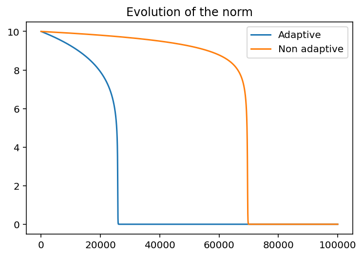
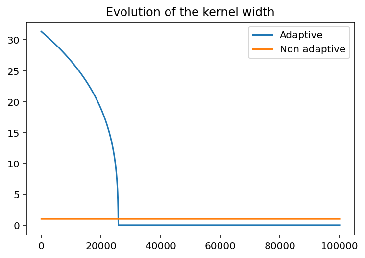
Figure 3: Evolution of the norm of the mean $\mu_{t}$ of the Gaussian distribution $\pi_{\mu_{t},\sigma}$ according to a gradient flow on the mean $\mu_{t}$ w.r.t. $\mathrm{MMD}_{\alpha_{t}}$. In the adaptive case $\alpha_{t}$ is given by Proposition 3.1 while in the non adaptive case, $\alpha_{t}=\alpha_{0}=1$. In our experiment we consider $d=1$ and $\sigma=1$, for illustration purposes.

Appendix G Image generation samples

G.1 CIFAR10 samples

Samples from $\mathrm{DMMD}$ with NFE=100 and NFE=250 are given in Figure 4. Samples from $\mathrm{DMMD}$ with NFE=100 and from $a$-$\mathrm{DMMD}$ with NFE=50 are given in Figure 5.

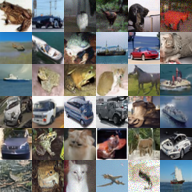
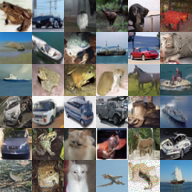
Figure 4: CIFAR-10 samples from $\mathrm{DMMD}$ with NFE=250 on the left and with NFE=100 on the right

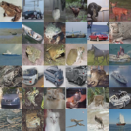
Figure 5: CIFAR-10 samples from $\mathrm{DMMD}$ with NFE=100 on the left and samples from the $a$-$\mathrm{DMMD}$-$e$ with NFE=50 on the right

G.2 Additional datasets samples

Samples for MNIST are given in Figure 6, for CELEB-A (64x64) are given in Figure 7 and for LSUN Church (64x64) are given in Figure 8.

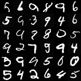
Figure 6: $\mathrm{DMMD}$ samples for MNIST.

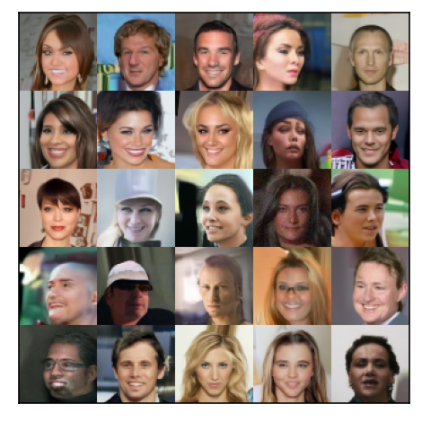
Figure 7: $\mathrm{DMMD}$ samples for CELEB-A (64x64).

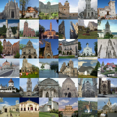
Figure 8: $\mathrm{DMMD}$ samples for LSUN Church (64x64).

References

- Aiello et al. (2023) Aiello, E., Valsesia, D., and Magli, E. Fast inference in denoising diffusion models via mmd finetuning, 2023.
- Altekrüger et al. (2023) Altekrüger, F., Hertrich, J., and Steidl, G. Neural wasserstein gradient flows for maximum mean discrepancies with riesz kernels, 2023.
- Ambrosio et al. (2008) Ambrosio, L., Gigli, N., and Savaré, G. Gradient Flows in Metric Spaces and in the Space of Probability Measures. Lectures in Mathematics ETH Zürich. Birkhäuser, 2. ed edition, 2008. ISBN 978-3-7643-8722-8 978-3-7643-8721-1. OCLC: 254181287.
- Ansari et al. (2021) Ansari, A. F., Ang, M. L., and Soh, H. Refining deep generative models via discriminator gradient flow, 2021.
- Arbel et al. (2018) Arbel, M., Sutherland, D. J., Bińkowski, M., and Gretton, A. On gradient regularizers for mmd gans. Advances in neural information processing systems, 31, 2018.
- Arbel et al. (2019) Arbel, M., Korba, A., Salim, A., and Gretton, A. Maximum mean discrepancy gradient flow, 2019.
- Arbel et al. (2021) Arbel, M., Zhou, L., and Gretton, A. Generalized energy based models, 2021.
- Arjovsky et al. (2017) Arjovsky, M., Chintala, S., and Bottou, L. Wasserstein gan, 2017.
- Arora et al. (2017) Arora, S., Ge, R., Liang, Y., Ma, T., and Zhang, Y. Generalization and equilibrium in generative adversarial nets (gans), 2017.
- Bińkowski et al. (2021) Bińkowski, M., Sutherland, D. J., Arbel, M., and Gretton, A. Demystifying mmd gans, 2021.
- Bortoli (2023) Bortoli, V. D. Convergence of denoising diffusion models under the manifold hypothesis, 2023.
- Brock et al. (2019) Brock, A., Donahue, J., and Simonyan, K. Large scale gan training for high fidelity natural image synthesis, 2019.
- Brown et al. (2022) Brown, B. C., Caterini, A. L., Ross, B. L., Cresswell, J. C., and Loaiza-Ganem, G. The union of manifolds hypothesis and its implications for deep generative modelling. arXiv preprint arXiv:2207.02862, 2022.
- Che et al. (2021) Che, T., Zhang, R., Sohl-Dickstein, J., Larochelle, H., Paull, L., Cao, Y., and Bengio, Y. Your gan is secretly an energy-based model and you should use discriminator driven latent sampling, 2021.
- Chen et al. (2022) Chen, S., Chewi, S., Li, J., Li, Y., Salim, A., and Zhang, A. R. Sampling is as easy as learning the score: theory for diffusion models with minimal data assumptions. arXiv preprint arXiv:2209.11215, 2022.
- Fan et al. (2022) Fan, J., Zhang, Q., Taghvaei, A., and Chen, Y. Variational wasserstein gradient flow, 2022.
- Fefferman et al. (2016) Fefferman, C., Mitter, S., and Narayanan, H. Testing the manifold hypothesis. Journal of the American Mathematical Society, 29(4):983–1049, 2016.
- Franceschi et al. (2022) Franceschi, J.-Y., de Bézenac, E., Ayed, I., Chen, M., Lamprier, S., and Gallinari, P. A neural tangent kernel perspective of gans, 2022.
- Franceschi et al. (2023) Franceschi, J.-Y., Gartrell, M., Santos, L. D., Issenhuth, T., de Bézenac, E., Chen, M., and Rakotomamonjy, A. Unifying gans and score-based diffusion as generative particle models, 2023.
- Genevay et al. (2018) Genevay, A., Peyre, G., and Cuturi, M. Learning generative models with sinkhorn divergences. In Proceedings of the Twenty-First International Conference on Artificial Intelligence and Statistics, volume 84 of Proceedings of Machine Learning Research, pp. 1608–1617. PMLR, 2018.
- Glaser et al. (2021) Glaser, P., Arbel, M., and Gretton, A. Kale flow: A relaxed kl gradient flow for probabilities with disjoint support, 2021.
- Goodfellow et al. (2014) Goodfellow, I. J., Pouget-Abadie, J., Mirza, M., Xu, B., Warde-Farley, D., Ozair, S., Courville, A., and Bengio, Y. Generative adversarial networks, 2014.
- Gretton et al. (2012) Gretton, A., Borgwardt, K. M., Rasch, M. J., Schölkopf, B., and Smola, A. A kernel two-sample test. Journal of Machine Learning Research, 13(25):723–773, 2012. URL http://jmlr.org/papers/v13/gretton12a.html.
- Gulrajani et al. (2017) Gulrajani, I., Ahmed, F., Arjovsky, M., Dumoulin, V., and Courville, A. Improved training of wasserstein gans, 2017.
- Hagemann et al. (2023) Hagemann, P., Hertrich, J., Altekrüger, F., Beinert, R., Chemseddine, J., and Steidl, G. Posterior sampling based on gradient flows of the mmd with negative distance kernel, 2023.
- Heng et al. (2023) Heng, A., Ansari, A. F., and Soh, H. Deep generative wasserstein gradient flows, 2023. URL https://openreview.net/forum?id=zjSeBTEdXp1.
- Hertrich et al. (2023) Hertrich, J., Wald, C., Altekrüger, F., and Hagemann, P. Generative sliced mmd flows with riesz kernels, 2023.
- Heusel et al. (2018) Heusel, M., Ramsauer, H., Unterthiner, T., Nessler, B., and Hochreiter, S. Gans trained by a two time-scale update rule converge to a local nash equilibrium, 2018.
- Ho et al. (2020) Ho, J., Jain, A., and Abbeel, P. Denoising diffusion probabilistic models, 2020.
- Ho et al. (2022) Ho, J., Chan, W., Saharia, C., Whang, J., Gao, R., Gritsenko, A., Kingma, D. P., Poole, B., Norouzi, M., Fleet, D. J., et al. Imagen video: High definition video generation with diffusion models. arXiv preprint arXiv:2210.02303, 2022.
- Hyvärinen (2005) Hyvärinen, A. Estimation of non-normalized statistical models by score matching. Journal of Machine Learning Research, 6(24):695–709, 2005. URL http://jmlr.org/papers/v6/hyvarinen05a.html.
- Jacot et al. (2020) Jacot, A., Gabriel, F., and Hongler, C. Neural tangent kernel: Convergence and generalization in neural networks, 2020.
- Jordan et al. (1998) Jordan, R., Kinderlehrer, D., and Otto, F. The variational formulation of the fokker–planck equation. SIAM Journal on Mathematical Analysis, 29(1):1–17, 1998. doi: 10.1137/S0036141096303359. URL https://doi.org/10.1137/S0036141096303359.
- Karras et al. (2020a) Karras, T., Aittala, M., Hellsten, J., Laine, S., Lehtinen, J., and Aila, T. Training generative adversarial networks with limited data, 2020a.
- Karras et al. (2020b) Karras, T., Laine, S., Aittala, M., Hellsten, J., Lehtinen, J., and Aila, T. Analyzing and improving the image quality of stylegan, 2020b.
- Kingma & Ba (2017) Kingma, D. P. and Ba, J. Adam: A method for stochastic optimization, 2017.
- Kodali et al. (2017) Kodali, N., Abernethy, J., Hays, J., and Kira, Z. On convergence and stability of gans, 2017.
- Krizhevsky et al. (2009) Krizhevsky, A., Hinton, G., et al. Learning multiple layers of features from tiny images. 2009.
- Le et al. (2023) Le, M., Vyas, A., Shi, B., Karrer, B., Sari, L., Moritz, R., Williamson, M., Manohar, V., Adi, Y., Mahadeokar, J., et al. Voicebox: Text-guided multilingual universal speech generation at scale. arXiv preprint arXiv:2306.15687, 2023.
- Lecun et al. (1998) Lecun, Y., Bottou, L., Bengio, Y., and Haffner, P. Gradient-based learning applied to document recognition. Proceedings of the IEEE, 86(11):2278–2324, 1998. doi: 10.1109/5.726791.
- Li et al. (2017) Li, C.-L., Chang, W.-C., Cheng, Y., Yang, Y., and Póczos, B. Mmd gan: Towards deeper understanding of moment matching network, 2017.
- Li & van der Schaar (2024) Li, Y. and van der Schaar, M. On error propagation of diffusion models, 2024.
- Liu et al. (2020) Liu, M.-Y., Huang, X., Yu, J., Wang, T.-C., and Mallya, A. Generative adversarial networks for image and video synthesis: Algorithms and applications, 2020.
- Liu et al. (2015) Liu, Z., Luo, P., Wang, X., and Tang, X. Deep learning face attributes in the wild, 2015.
- Mescheder et al. (2018) Mescheder, L., Geiger, A., and Nowozin, S. Which training methods for gans do actually converge? In International conference on machine learning, pp. 3481–3490. PMLR, 2018.
- Muller (1997) Muller, A. Integral probability metrics and their generating classes of functions. volume 29, pp. 429–443. Advances in Applied Probability, 1997.
- Nowozin et al. (2016) Nowozin, S., Cseke, B., and Tomioka, R. f-gan: Training generative neural samplers using variational divergence minimization, 2016.
- Pidstrigach (2022) Pidstrigach, J. Score-based generative models detect manifolds. Advances in Neural Information Processing Systems, 35:35852–35865, 2022.
- Poole et al. (2022) Poole, B., Jain, A., Barron, J. T., and Mildenhall, B. Dreamfusion: Text-to-3d using 2d diffusion. arXiv preprint arXiv:2209.14988, 2022.
- Rombach et al. (2022) Rombach, R., Blattmann, A., Lorenz, D., Esser, P., and Ommer, B. High-resolution image synthesis with latent diffusion models, 2022.
- Ronneberger et al. (2015) Ronneberger, O., Fischer, P., and Brox, T. U-net: Convolutional networks for biomedical image segmentation, 2015.
- Saharia et al. (2022) Saharia, C., Chan, W., Saxena, S., Li, L., Whang, J., Denton, E. L., Ghasemipour, K., Gontijo Lopes, R., Karagol Ayan, B., Salimans, T., et al. Photorealistic text-to-image diffusion models with deep language understanding. Advances in Neural Information Processing Systems, 35:36479–36494, 2022.
- Salimans et al. (2016) Salimans, T., Goodfellow, I., Zaremba, W., Cheung, V., Radford, A., and Chen, X. Improved techniques for training gans, 2016.
- Santambrogio (2015) Santambrogio, F. Optimal transport for applied mathematicians. Birkäuser, NY, 55(58-63):94, 2015.
- Sauer et al. (2023) Sauer, A., Lorenz, D., Blattmann, A., and Rombach, R. Adversarial diffusion distillation. arXiv preprint arXiv:2311.17042, 2023.
- Schölkopf & Smola (2018) Schölkopf, B. and Smola, A. J. Learning with Kernels: Support Vector Machines, Regularization, Optimization, and Beyond. The MIT Press, 06 2018. ISBN 9780262256933. doi: 10.7551/mitpress/4175.001.0001. URL https://doi.org/10.7551/mitpress/4175.001.0001.
- Sohl-Dickstein et al. (2015) Sohl-Dickstein, J., Weiss, E. A., Maheswaranathan, N., and Ganguli, S. Deep unsupervised learning using nonequilibrium thermodynamics, 2015.
- Song et al. (2020) Song, Y., Sohl-Dickstein, J., Kingma, D. P., Kumar, A., Ermon, S., and Poole, B. Score-based generative modeling through stochastic differential equations. arXiv preprint arXiv:2011.13456, 2020.
- Song et al. (2023) Song, Y., Dhariwal, P., Chen, M., and Sutskever, I. Consistency models. arXiv preprint arXiv:2303.01469, 2023.
- Szegedy et al. (2014) Szegedy, C., Liu, W., Jia, Y., Sermanet, P., Reed, S., Anguelov, D., Erhan, D., Vanhoucke, V., and Rabinovich, A. Going deeper with convolutions, 2014.
- Tenenbaum et al. (2000) Tenenbaum, J. B., Silva, V. d., and Langford, J. C. A global geometric framework for nonlinear dimensionality reduction. science, 290(5500):2319–2323, 2000.
- Villani (2008) Villani, C. Optimal Transport: Old and New. Grundlehren der mathematischen Wissenschaften. Springer Berlin Heidelberg, 2008. ISBN 9783540710509. URL https://books.google.co.uk/books?id=hV8o5R7_5tkC.
- Vincent (2011) Vincent, P. A connection between score matching and denoising autoencoders. Neural Computation, 23(7):1661–1674, 2011.
- Watson et al. (2022) Watson, J. L., Juergens, D., Bennett, N. R., Trippe, B. L., Yim, J., Eisenach, H. E., Ahern, W., Borst, A. J., Ragotte, R. J., Milles, L. F., et al. Broadly applicable and accurate protein design by integrating structure prediction networks and diffusion generative models. BioRxiv, pp. 2022–12, 2022.
- Xiao et al. (2022) Xiao, Z., Kreis, K., and Vahdat, A. Tackling the generative learning trilemma with denoising diffusion gans, 2022.
- Xu et al. (2023) Xu, Y., Zhao, Y., Xiao, Z., and Hou, T. Ufogen: You forward once large scale text-to-image generation via diffusion gans. arXiv preprint arXiv:2311.09257, 2023.
- Yang et al. (2023) Yang, Z., Feng, R., Zhang, H., Shen, Y., Zhu, K., Huang, L., Zhang, Y., Liu, Y., Zhao, D., Zhou, J., and Cheng, F. Eliminating lipschitz singularities in diffusion models, 2023.
- Yu et al. (2016) Yu, F., Seff, A., Zhang, Y., Song, S., Funkhouser, T., and Xiao, J. Lsun: Construction of a large-scale image dataset using deep learning with humans in the loop, 2016.
- Zhang et al. (2018) Zhang, P., Liu, Q., Zhou, D., Xu, T., and He, X. On the discrimination-generalization tradeoff in gans. In 6th International Conference on Learning Representations, 2018.