Hamiltonian and Liouvillian learning in weakly-dissipative quantum many-body systems

Abstract

We discuss Hamiltonian and Liouvillian learning for analog quantum simulation from non-equilibrium quench dynamics in the limit of weakly dissipative many-body systems. We present various strategies to learn the operator content of the Hamiltonian and the Lindblad operators of the Liouvillian. We compare different ansätze based on an experimentally accessible ‘learning error’ which we consider as a function of the number of runs of the experiment. Initially, the learning error decreasing with the inverse square root of the number of runs, as the error in the reconstructed parameters is dominated by shot noise. Eventually the learning error remains constant, allowing us to recognize missing ansatz terms. A central aspect of our approach is to (re-)parametrize ansätze by introducing and varying the dependencies between parameters. This allows us to identify the relevant parameters of the system, thereby reducing the complexity of the learning task. Importantly, this (re-)parametrization relies solely on classical post-processing, which is compelling given the finite amount of data available from experiments. A distinguishing feature of our approach is the possibility to learn the Hamiltonian, without the necessity of learning the complete Liouvillian, thus further reducing the complexity of the learning task. We illustrate our method with two, experimentally relevant, spin models.

I Introduction

Controllable quantum many-body systems, when scaled to a large number of particles, hold the potential to function as quantum computers or quantum simulators, addressing computational problems that are considered intractable for classical computers [1]. Remarkable progress has been reported recently in building quantum simulators, as programmable special-purpose quantum devices, to solve quantum many-body problems efficiently, which finds applications in condensed matter [2], high-energy physics [3], and quantum chemistry [4], in both equilibrium and non-equilibrium dynamics. Quantum simulation can be realized as analog or digital quantum simulators. In analog simulation, a target Hamiltonian finds a natural implementation on a quantum device, exemplified by ultracold bosonic and fermionic atoms in optical lattices as Hubbard models [5, 6, 7, 8], or spin models with trapped ions [9, 10, 11, 12], Rydberg tweezer arrays [13, 14, 15, 16], and superconducting qubits [17, 18, 19]. The unique feature of analog quantum simulators is the scalability to large particle numbers. In contrast, digital quantum simulation [20] represents the time evolution of a given many-body Hamiltonian using a freely programmable sequence of Trotter steps implemented via single and multi-qubit entangling quantum gates.

An outstanding challenge in quantum simulation is the ability to predict properties of many-body observables with controlled error while scaling to a regime of potential quantum advantage [21, 22, 23, 24]. Given the increase of complexity of these systems, methods to characterize, and thus verify, the proper functioning of quantum simulators are required [25, 26, 27]. This includes verification, that the correct many-body Hamiltonians are being implemented, and a complete characterization of (weak) decoherence due to unwanted couplings to an environment or fluctuating external fields. In the present paper, we approach this goal by studying Hamiltonian and Liouvillian learning for analog quantum simulators. Previous works have studied various scenarios for Hamiltonian and Liouvillian learning [28, 29, 30, 31, 32, 33, 34, 35, 33, 34, 36, 37, 38], for instance, by comparing with a trusted simulator [28], or based on the preparation of steady states [30, 31, 32, 33, 34]. Alternative approaches are based on dynamics in (long-time) quenches [35, 33, 34, 36], or the estimation of the time-derivatives of few-qubit observables from short-time evolution [37, 38].

Here, we will be interested in Hamiltonian and Liouvillian learning from dynamics in long-time quenches of product states, with only few experimental requirements such as the preparation of product states, and product measurements. We assume that the dynamics of the experimental quantum simulator is described by a master equation, where the Hamiltonian acts as a generator of the coherent many-body dynamics, while Lindbladian terms model the noise. The goal of Hamiltonian and Liouvillian learning is to learn the operator structure, reminiscent of a principal component analysis [39], of both the many-body Hamiltonian, as one-, two- or few-body interaction terms including their couplings, and the quantum jump operators in the dissipative Liouvillian, representing local or non-local (global) quantum and classical noise. The scalability and efficiency of Hamiltonian and Liouvillian learning are related to the assumption that physical Hamiltonians and Liouvillians will only involve few-body interactions and quantum jump operators, leading to a polynomial scaling of the number of terms to be learned with system size.

Our study below discusses and compares various scenarios and strategies of Hamiltonian and Liouvillian learning, which we illustrate by simulating learning protocols for various model cases. Our work is motivated by present trapped-ion experiments, where quantum simulators realize 1D interacting weakly dissipative spin-1/2 chains. This allows quench experiments to be performed, and we will be interested in learning the Hamiltonian and Liouvillian from experimental quench data observed at various quench times. Learning the Hamiltonian and Liouvillian requires many experimental runs. In each run projective measurements of spins are performed in various bases, allowing to measure multi-spin correlation functions up to shot noise. In addition, learning protocols will prepare many initial states, which in our case can be pure or mixed, thus resulting in stability against state-preparation errors. A central aspect of our study below will thus be an investigation of the experimentally measurable learning error of Hamiltonian and Liouvillian, and its scaling with the number of measurement runs.

The paper is structured as follows. Section II outlines the specific scenario we’re examining and the core theoretical concepts involved. Section II.1 establishes some constraints on the system’s Hamiltonian and Liouvillian, measurable through simple quench experiments. We then present the main equations that enable us to infer the Hamiltonian and Liouvillian from experimental data in Sections II.2 to II.4, and the effect of shot-noise in Section II.5. Furthermore, we propose and discuss various strategies for Hamiltonian and Liouvillian learning in Section II.6. We compare different ansätze for the operator content, using an experimentally measurable quantity, which we identify as a learning error. These ansätze are derived by re-parametrizing our ansatz, typically involving data recycling and classical post-processing. The learning process can be divided into two phases as a function of experimental runs $N_{\rm runs}$: in the early phase, the learning error is dominated by shot-noise and decays $\sim N_{\rm runs}^{-1/2}$. In the later phase, systematic errors become dominant due to missing terms in the ansatz, or an insufficient ansatz. This leads to a constant learning error independent of the number of measurements, indicating the need to extend our ansatz. Finally, in Section III, we showcase learning protocols for various model scenarios through numerical simulations.

II Hamiltonian and Liouvillian Learning of Many-Body Systems

II.1 Background

We consider analog quantum simulation in a regime, where the engineered quantum many-body system of interest is weakly coupled to a decohering environment. We assume that the system dynamics is described by a master equation with Lindblad form [40],

$$\frac{\mathrm{d}}{\mathrm{d}t}\varrho = -i[H,\varrho]+\frac{1}{2}\sum_{k}\gamma_{k}\left([l_{k}\varrho,l_{k}^{\dagger}]+[l_{k},\varrho l_{k}^{\dagger}]\right)$$

$$\equiv \mathcal{L}_{H}(\varrho)+\mathcal{L}_{D}(\varrho),$$

comprising a coherent term $\mathcal{L}_{H}(\varrho)=-i[H,\varrho]$ with many-body Hamiltonian $H$ and a dissipative term $\mathcal{L}_{D}$, referred to as the Liouvillian. The Lindblad quantum jump operators $l_{k}$ describe dissipative processes coupling the system to an environment. Here, $\gamma_{k}\geq 0$ is the physical domain for the corresponding damping rates, where the dynamics is described by a completely positive and trace-preserving map [41, 42]. Throughout this work, we assume that the Hamiltonian and the Liouvillian are time-independent. In typical experimental settings, the Hamiltonian terms are significantly larger than dissipative processes $\norm{H}\gg\gamma_{k}$.

Below we will be interested in analog quantum simulation of spin-1/2 systems, as implemented with trapped ions [9, 10, 11, 12], Rydberg tweezer arrays [14, 15, 16], or superconducting circuits [17, 19]. An illustrative example of a two-local spin-Hamiltonian in one spatial dimension, which we have in mind, is given by

$$H = \sum_{i=1}^{N-1}J_{i,i+1}^{z}\sigma_{i}^{z}\sigma_{i+1}^{z}+\sum_{i=1}^{N-2}J_{i,i+2}^{z}\sigma_{i}^{z}\sigma_{i+2}^{z}$$

$$\quad+B_{x}\sum_{i=1}^{N}\sigma_{i}^{x}+B_{z}\sum_{i=1}^{N}\sigma_{i}^{z},$$

which describes a next-nearest-neighbor Ising model of $N$ spins with longitudinal- and transverse fields.

The Liouvillian, $\mathcal{L}_{D}$, in Eq. (II.1) is defined by its Lindblad, or quantum jump operators $l_{k}$. Examples of Lindblad operators, that typically appear in experiments, include spontaneous emission, described by local Lindblad operators $l_{k}=\sigma^{-}_{k}$, or local dephasing, represented by $l_{k}=\sigma^{z}_{k}$. Besides local dissipation, we will be interested in identifying the presence of collective dissipative effects, for instance, in the form of collective dephasing caused by globally fluctuating laser fields or effective magnetic fields, leading to a collective Lindblad operator $l=\sum_{k}\sigma^{z}_{k}$.

Before we proceed with the discussion, we need to establish certain conditions on the Hamiltonian and Liouvillian of the system. For a time-independent observable, $O$, Ehrenfest’s theorem, in the context of Eq. (II.1), states that

$$\frac{\mathrm{d}}{\mathrm{d}t}\expectationvalue*{O}=\expectationvalue{-i[O,H]}+\frac{1}{2}\sum_{k}\gamma_{k}\langle l_{k}^{\dagger}[O,l_{k}]+[l_{k}^{\dagger},O]l_{k}\rangle,$$ (3)

where $\expectationvalue*{X}=\tr[X\varrho]$, for any state $\varrho$. Here, we consider $O=H$ which leads to

$$\expectationvalue{H}_{T}-\expectationvalue{H}_{0}=\\ \frac{1}{2}\sum_{k}\gamma_{k}\int_{0}^{T}\expectationvalue*{l_{k}^{\dagger}[H,l_{k}]+[l_{k}^{\dagger},H]l_{k}}_{t}\mathrm{d}t.$$ (4)

It describes the total energy loss during a quench of duration $T$. Here, $\expectationvalue{X}_{t}=\tr[X\exp{t(\mathcal{L}_{H}+\mathcal{L}_{D})}\varrho(0)]$. If $\gamma_{k}=0$ for all $k$, this equation indicates the conservation of energy. In our Hamiltonian and Liouvillian learning protocol, Eq. (4) will play a crucial role. We will generalize the protocol of Ref. [35] for Hamiltonian learning in the absence of dissipation, and present it in a form particularly suited for learning $H$ and $\cal L_{D}$ in the limit of weak dissipation.

As a final remark, let us elaborate on the experimental procedure that we are considering which can be used to probe the conditions in Eqs. (3) and (4) (see also Fig. 1 for an illustration). Starting from a product state, $\ket{\psi(0)}=\ket{\psi_{1}}\otimes\dots\otimes\ket{\psi_{N}}$, which can be experimentally prepared with high fidelity, one evolves the state under the Hamiltonian and Liouvillian for some time $t$. The resulting state, $\varrho(t)=\exp{t(\mathcal{L}_{H}+\mathcal{L}_{D})}(\varrho(0))$, is measured in a product basis, for instance, in the Pauli basis. Clearly, the limiting quantity, here, and in the following, will be the total number of runs of quench experiments, which we will denote by $N_{\rm runs}$. Given, however, that many-body Hamiltonians typically consist of a few quasi-local operators, many of the required measurements can be carried out simultaneously, i.e., in a single run, using classical post-processing.

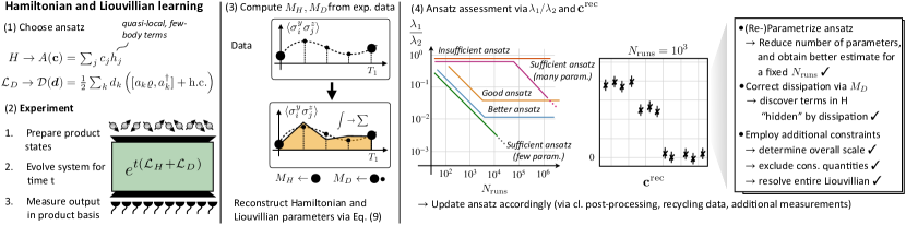
Figure 1: Our learning procedure starts by choosing an ansatz for the operator structure of the Hamiltonian and Liouvillian. The experimental procedure requires the preparation of multiple product states. These states are evolved under the unknown dynamics for different times $T\in\{T_{i}\}$ (and multiple intermediate times), followed by a measurement of a few quasi-local, few-body correlation functions, most of which can be measured simultaneously. One obtains time-discretized estimates of time-traces of observables, where times $T_{i}$ are measured using a larger measurement budget compared to intermediate times. The constraint matrix $M_{H}$ is estimated from measurements at times $T_{i}$. The constraint matrix $M_{D}$ is obtained from estimating the integrals in Eq. (8) using Simpson’s rule from measurements at intermediate times. To assess the ansatz, one considers our figure of merit $\lambda_{1}/\lambda_{2}$, or the reconstructed parameters $\bm{c}^{\rm rec}$ and $\bm{d}^{\rm rec}$, for which one can compute error bars using bootstrapping. In early stages of the learning procedure $\lambda_{1}/\lambda_{2}$ decreases with $N_{\rm runs}^{-1/2}$, indicating that the dominant source of error is shot noise. In later stages, $\lambda_{1}/\lambda_{2}$ remains constant, indicating that our ansatz is missing terms. Based on this assessment, and comparing different ansätze, we can identify an ansatz comprising the dominant operator content and few relevant parameters, resulting in an early shot-noise scaling and a low plateau. On top of that, one may also learn the overall scale of $H$, exclude conserved quantities, or learn the complete Liouvillian by including additional constraints.

II.2 Hamiltonian and Liouvillian learning

Often in, an experimental setting, the detailed structure of the Hamiltonian and the Liouvillian are unknown. We present here a method to learn the operator content of $H$ and $\mathcal{L}_{D}$, and the corresponding parameters from experimental data. For instance, in the context of the spin system in and below Eq. (II.1), identifying the operator content means identifying the Pauli operators that appear in the decomposition of $H$ and the Lindblad operators $l_{k}$.

We start by choosing an ansatz for the operator content for the Hamiltonian and Liouvillian. Specifically, as an ansatz for $H$ we choose

$$A(\bm{c})=\sum_{j=1}^{n}c_{j}h_{j},$$ (5)

with parameters $\bm{c}=(c_{1},\dots,c_{n})$, and $h_{j}$ traceless and hermitian for all $j$. As an example, one could choose the $h_{j}$ to be few-body Pauli operators. As an ansatz for the Liouvillian we choose

$$\mathcal{D}(\bm{d})=\frac{1}{2}\sum_{k}d_{k}\left([a_{k}\varrho,a_{k}^{\dagger}]+[a_{k},\varrho a_{k}^{\dagger}]\right),$$ (6)

with Lindblad operators $\{a_{k}\}$, and parameterized by the corresponding non-negative dissipation rates, $\bm{d}=(d_{1},d_{2},\ldots)$. Inserting our ansatz into Eq. (4), and imposing the resulting constraint for a set of initial (product) states $\{\varrho_{i}\}$, where $i=1,\dots,p$, leads to the following simple matrix equation 

$$[M_{H}+M_{D}(\bm{d})]\bm{c}=0.$$ (7)

The matrices $M_{H}$ and $M_{D}(\bm{d})$ are $p\times n$ matrices defined by $M_{H}=(M)_{ij}=\expectationvalue*{h_{j}}_{i,0}-\expectationvalue*{h_{j}}_{i,T}$, and $M_{D}(\bm{d})=\sum_{k}d_{k}M^{(k)}$, with

$$[M^{(k)}]_{ij}=\int_{0}^{T}\expectationvalue*{a_{k}^{\dagger}[h_{j},a_{k}]+[a_{k}^{\dagger},h_{j}]a_{k}}_{i,t}\mathrm{d}t,$$ (8)

and $\expectationvalue{X}_{i,t}=\tr[X\varrho_{i}(t)]$. We emphazise here, that in case $h_{j}$ and $l_{k}$ are Pauli operators, the expectation values in Eq. (8) evaluate to $\alpha\expectationvalue{h_{j}}$, where $\alpha=0$ if $[l_{k},h_{j}]=0$, and $\alpha=-4$ otherwise . Moreover, as Eq. (7) also holds in case the states $\{\varrho_{i}\}$ are mixed, our protocol, similar to the Hamiltonian learning protocol in Ref. [35], is resistant to state-preparation errors.

In the discussion above, we have implicitly assumed that our ansatz is chosen such as to contain the Hamiltonian and Liouvillian, i.e., there exist vectors $\bm{c}^{H}$, and $\bm{d}^{\mathcal{L}}$, such that $A(\bm{c}^{H})=H$, and $\mathcal{D}(\bm{d}^{\mathcal{L}})=\mathcal{L}_{D}$. However, in practice we do not expect this to be the case, and we will call such an ansatz insufficient . Nevertheless, we can determine the parameters of our ansatz minimizing the violation of the energy conditions in Eq. (4). This amounts to minimizing the squared residuals in Eq. (7), i.e.,

$$(\bm{c}^{\rm rec},\bm{d}^{\rm rec})=\operatorname*{arg\,min}_{(\bm{c},\bm{d}):\norm{\bm{c}}=1,\bm{d}\geq 0}\norm{\quantity[M_{H}+M_{D}(\bm{d})]\bm{c}},$$ (9)

where $\|\bm{x}\|$ denotes the $2$-norm. Computing the minimum of the cost function in Eq. (9) corresponds to finding non-negative dissipation rates $\bm{d}^{\rm rec}$ for which the smallest singular value, $\lambda_{1}$, of the constraint matrix $M_{H}+M_{D}(\bm{d})$ attains its minimum. The corresponding $\bm{c}^{\rm rec}$ is then the right-singular vector corresponding to $\lambda_{1}$. In the following we will denote the singular vectors of the constraint matrix by $\lambda_{n}\geq\dots\geq\lambda_{2}\geq\lambda_{1}\geq 0$.

In an experiment, the constraint matrices $M_{H}$ and $M_{D}(\bm{d})$ need to be estimated from data. The matrix $M_{H}$ can be determined experimentally by measuring $\expectationvalue{h_{j}}_{0}$ and $\expectationvalue{h_{j}}_{T}$ for all input states $i$. As the $h_{j}$ are few-body operators many of them commute and can thus be measured jointly. To obtain $M_{D}$, one needs to estimate the integrals in Eq. (8). Here, we use the composite Simpson’s rule which approximates an integral as a series of parabolic segments between $N_{t}$ equally spaced points $t_{m}=m\cdot\Delta t$, with $m\in 0,\dots,N_{t}$ and $\Delta t=T/N_{t}$. It reads

$$\int_{0}^{T}\expectationvalue*{h}_{t}\mathrm{d}t\approx\frac{1}{3}\Delta t\left[\expectationvalue*{h}_{0}+4\sum_{k=0}^{N_{t}/2}\expectationvalue*{h}_{t_{2k-1}}\right.\\ \left.+2\sum_{k=0}^{N_{t}/2-1}\expectationvalue*{h}_{t_{2k}}+\expectationvalue*{h}_{T}\right].$$ (10)

Therefore, the estimation of $M_{D}(\bm{d})$ requires additional measurements at times $t_{m}\in[0,T]$ of operators $h_{j}$, see also Fig. 1 for an illustration. In the following, we choose a sufficiently small time step $\Delta t$ to ensure that errors arising from discretizing the integral can be disregarded in comparison to shot-noise errors .

II.3 Learning the overall scale, and conserved quantities

When imposing Eq. (4) on numerous initial states in quench dynamics, it leads to a large number of constraints on the Hamiltonian and Liouvillian. However, it is worth noting that these conditions are not enough to uniquely specify the Hamiltonian. The conditions in Eq. (4) define the Hamiltonian only up to a scalar factor since they are linear in $H$. Additionally, these conditions apply to any operator $Q$ such that $[Q,H]=0$, which means they define a linear subspace within the space of Hermitian operators that contains all conserved quantities of $\mathcal{L}_{H}$. An ansatz, $A(\bm{c})$, then may contain the Hamiltonian, $H$, and other conserved quantities of $\mathcal{L}_{H}$ which admit a decomposition in the form of $A(\bm{c})$. For instance, if we choose our ansatz to be $k$-local, it contains at most $k$-local conserved quantities. An example, which we will also consider later, is the total magnetization in ion-trap experiments, $Q\sim\sum_{k}\sigma^{z}_{k}$, which is a sum of local operators.

So let us assume that an ansatz contains two linearly independent conserved quantities $H$, and $Q$, corresponding to two linearly independent vectors $\bm{c}^{H}$, and $\bm{c}^{Q}$, the generalization to more conserved quantities is straightforward. Then, by singular value decomposition, one obtains two right singular vectors $\{\bm{v},\bm{v}_{\perp}\}$, which both satisfy Eq. (7). Therefore, the corresponding singular values, $\lambda_{1}$ and $\lambda_{2}$, are degenerate, i.e., $\lambda_{1}=\lambda_{2}$. However, the right singular vectors must not necessarily correspond to $\bm{c}^{H}$ and $\bm{c}^{H}_{\perp}$. Thus, in the presence of conserved quantities, naively solving Eq. (9) would in general reconstruct the parameters of a linear combination of conserved quantities.

To single out $\bm{c}^{H}$ from this subspace, one needs to impose additional constraints that can only be fulfilled by $H$, but not by other conserved quantities, including scalar multiples of $H$. Such a constraint can be obtained from Ehrenfest’s theorem in Eq. (3) by inserting the ansatz $A(\bm{c})$ for $H$, and considering a generic observable, $O$, not commuting with $H$. This leads to additional constraints, which can only be satisfied by the Hamiltonian, and thus $\bm{c}^{H}$. We spell out the modified equations in Appendix A. The optimization problem in Eq. (9) is then modified to

$$(\bm{c}^{\rm rec},\bm{d}^{\rm rec})=\operatorname*{arg\,min}_{(\bm{c},\bm{d}):\bm{d}\geq 0}\norm{\matrixquantity(M(\bm{d})\\ \xi M^{\mathrm{\rm add}})\bm{c}-\matrixquantity(0\\ \xi\bm{b}(\bm{d}))},$$ (11)

where $M^{\rm add}$, and $\bm{b}(\bm{d})$ contain additional constraints determining the overall scale, and to single out $\bm{c}^{H}$ (see also Appendix A for explicit formulae for these constraints). Both can be estimated from quench experiments described above, requiring only measurements of few-body Pauli operators. Moreover, the auxiliary parameter $\xi$ controls the penalty that is added for violating the condition determining $H$ within the subspace of conserved quantities of $\mathcal{L}_{H}$. Choosing this parameter large enough allows us to reconstruct a $\bm{c}^{\rm rec}\approx\bm{c}^{H}$, with the correct overall scale, as a unique solution of Eq. (11). We emphasize, that by choosing the appropriate additional constraints, Eq. (11) can also be used to learn other conserved quantities of $\mathcal{L}_{H}$.

II.4 Learning the full Liouvillian

Since we have dissipative dynamics, one expects that accurately learning the Hamiltonian also requires learning all the individual dissipation rates. This is, however, not necessarily the case. In some cases, different dissipative processes give the same contribution to Eq. (4), and therefore, cannot be distinguished by the conditions in Eq. (4). This is a unique feature of our approach as it enables us to learn the Hamiltonian $H$, without having to learn the complete Liouvillian $\mathcal{L}_{D}$.

This feature can be understood already with a simple example of a single spin with Hamiltonian $H=\sigma_{y}$, and Liouvillian

$$\mathcal{L}_{D}(\varrho)=\frac{\gamma_{x}}{2}\left([\sigma_{x}\varrho,\sigma_{x}]+\text{h.c.}\right)+\frac{\gamma_{z}}{2}\left([\sigma_{z}\varrho,\sigma_{z}]+\text{h.c.}\right).$$ (12)

For simplicity, inserting the above Hamiltonian and Liouvillian as an ansatz in the condition in Eq. (4), leads to the following;

$$\expectationvalue{\sigma_{y}}_{T}-\expectationvalue{\sigma_{y}}_{0}=\frac{1}{2}\quantity[\sum_{k}\gamma_{k}]\int_{0}^{T}-4\expectationvalue{\sigma_{y}}_{t}\,\mathrm{d}t,$$ (13)

where the right-hand side only depends on the sum of dissipation rates. Moreover, the same condition is obtained for a Liouvillian with only $\sigma_{x}$, or $\sigma_{z}$ Lindblad operators. This has two consequences. Firstly, using these conditions one can learn the Hamiltonian without resolving individual dissipation rates. And secondly, one can learn the Hamiltonian with an insufficient ansatz for the Liouvillian. While this is only a simple illustrative example, we note that this also happens for experimentally relevant systems, such as, for instance, the long-range XY model, as we will illustrate in Section III.2.

More generally, the above feature can be summarized as follows. When inserting an ansatz into the conditions in Eq. (4), with the property discussed above, the resulting constraint matrices $\{M^{(k)}\}$ in Eq. (8), where $k$ labels the different Lindblad operators, become linearly dependent. Then, the decomposition $M_{D}(\bm{d})=\sum_{k}d_{k}M^{(k)}$ is not unique. This dependence leads to symmetries in the cost function in Eq. (9), such that the Hamiltonian $H$ can be learned exactly, for different dissipation rates $\bm{d}^{\mathrm{rec}}$. In order to learn the full Liouvillian and resolve individual dissipation rates, one needs to add additional constraints in the same way as one does for excluding conserved quantities and learning overall scale in Section II.3. This can then be phrased as an optimization problem of the form of Eq. (11), which we explain in detail in Appendix A. Moreover, we will show how to choose additional constraints to learn the full Liouvillian in Section III.2.

II.5 Effect of shot noise

In case the ansatz for the dynamics is sufficient, the only source of error is shot noise. Therefore, with a limited measurement budget one obtains a noisy estimate $\widetilde{M}(\bm{d})=M(\bm{d})+E(\bm{d})$, with an error matrix $E(\bm{d})$. Weyl’s inequality states the following bound on the perturbed singular value $\lambda_{1}$

$$\lambda_{1}[\widetilde{M}(\bm{d})]\leq\norm{E(\bm{d})}.$$ (14)

Therefore, in early stages of the learning procedure, one expects $\lambda_{1}$ to decrease $\sim N_{\rm runs}^{-1/2}$ as we increase the number of runs, $N_{\rm runs}$, in the experiment. Moreover, if an ansatz is insufficient, $\lambda_{1}$ is strictly bounded away from zero, even in the absence of shot noise. Thus, for $N_{\rm runs}$ sufficiently large, $\lambda_{1}$ will reach a plateau. Here, the dominant source of error will be systematic errors due to missing terms in our ansatz.

In case of a sufficient ansatz and without degeneracy of the smallest singular values, one can understand the role of the singular value $\lambda_{2}$. To this end, one considers the angle $\theta=\angle(\bm{c}^{H},\bm{c}^{\rm rec})$. It is a well known result in singular subspace perturbation theory, that the stability of a singular vector under perturbation depends on the gap between the corresponding singular value and the remainder of the spectrum, which is known as the Davis-Kahan-Wedin $\sin(\theta)$-theorem [47, 48]. For the case we consider this theorem establishes the following upper bound on the angle $\theta$ [48]

$$|\sin(\theta)|\leq\frac{\norm{E(\bm{d})}}{\delta}.$$ (15)

Here, $\delta=\lambda_{2}-\lambda_{1}^{\rm exact}$, and $\lambda_{1}^{\rm exact}=0$ for a sufficient ansatz. In case the elements of $E$ are i.i.d. Gaussian random variables one can establish average bounds on $\sin(\theta)$ [35]. However, we emphasize that the noise will in general be correlated due to the fact that we perform many of the required measurements in parallel. Moreover, the error matrix $E(\bm{d})$ is experimentally inaccessible. Nevertheless, we will demonstrate in the following, that the ratio $\lambda_{1}/\lambda_{2}$, which can be directly computed from experimental data, serves as a quantity to asses an ansatz. This figure of merit is motivated by the fact that $\lambda_{1}$ quantifies the violation of generalized energy conservation in Eq. (4) and that a larger gap $\delta=\lambda_{2}$ improves the upper bound in Eq. (15). As we will see below, the gap is typically larger for ansätze with fewer parameters.

II.6 Strategies for Hamiltonian and Liouvillian learning

A fundamental tension in Hamiltonian and Liouvillian learning is the tradeoff between the number of parameters of an ansatz, and the number of measurements that are required to estimate these parameters from experimental data. While complex ansätze, comprising many parameters, allows us to learn many aspects of the dynamics, they require a large measurement budget to reduce shot noise. In contrast, in the case of a limited measurement budget, it is quite useful to reduce the number of parameters to just a few relevant ones. This is also physically justified as many experimentally relevant Hamiltonians can be effectively characterized by only a few parameters, which may not even increase with system size. Illustrative examples include translationally invariant systems, or systems exhibiting algebraically decaying interactions. While ansätze with few parameters only require a small measurement budget, they are insufficient in the limit of an infinite number of measurements. However, as long as these insufficiencies are small, learning will be limited by shot noise. Therefore, our goal in the following is to find an ansatz comprising only few parameters and the dominant terms of the Hamiltonian and Liouvillian, which do not show any insufficiencies below our limited measurement budget.

To find this ansatz, we compare different ansätze by varying their operator content as well as their parametrization (see also Fig. 1(4) for an illustration of the following discussion). We emphasize that reparametrization can be done solely by classical post-processing of the data. To compare different ansätze, we will use the ratio $\lambda_{1}/\lambda_{2}$ as a quantifier for the learning error of an ansatz. One expects that in the early stages of the learning procedure, this ratio decreases with $N_{\rm runs}^{-1/2}$, as shot noise is the dominant source of error. In this regime, we will consider the reconstructed parameters $\bm{c}^{\rm rec}$ and $\bm{d}^{\rm rec}$, for which we compute error bars using bootstrapping methods. This allows us to identify dominant terms in the Hamiltonian and Liouvillian, thus learning the dominant operator structure. In later stages of the learning procedure, one expects that $\lambda_{1}/\lambda_{2}$ reaches a plateau due to the insufficient of the ansatz. In that case, we extend our ansatz, for instance, by adding additional operators to the Hamiltonian, or additional Lindblad operators to the Liouvillian. When comparing different ansätze, we choose the one which minimizes $\lambda_{1}/\lambda_{2}$. This results in an ansatz containing only few parameters and small missing terms, i.e., with an early shot-noise scaling, and a low plateau.

Reparametrizing an ansatz involves adjusting the structure of its parameters, while leaving the operator content unchanged. For instance, we will use reparametrization to reduce the number of parameters, resulting in a transformation of the vector of Hamiltonian parameters $\bm{c}$ with $n$ entries, to a vector $\bm{c}_{G}$ with with fewer entries, $\tilde{n}\leq n$. A simple way to achieve this is by transforming the vector $\bm{c}$ and the constraint matrices $M_{H}$ and $M_{D}(\bm{d})$ via a parametrization matrix, $G$, encoding dependencies between the parameters. This results in a transformation

$$\bm{c} \mapsto\bm{c}_{G}=G^{T}\bm{c},$$ (16)

$$M_{H} \mapsto M^{H}_{G}=M_{H}G,$$ (17)

$$M_{D}(\bm{d}) \mapsto M^{D}_{G}(\bm{d})=M_{D}(\bm{d})G.$$ (18)

Here, $G$ is an isometry from $\mathbb{R}^{\tilde{n}}$ to $\mathbb{R}^{n}$, and $\tilde{n}\leq n$, as $G^{T}G=\mathds{1}_{\tilde{n}\times\tilde{n}}$, and $GG^{T}$ a projector onto the image of $G$ (see Appendix B for details). The projector $GG^{T}$ projects onto a subspace spanned by vectors $\bm{c}$, with $n$ entries, which admit the dependencies encoded in $G$, for instance, translation invariance. Reconstructing the parameters of the reparametrized ansatz then amounts to solving

$$\bm{c}^{\mathrm{rec}}_{G}=\underset{\bm{c}_{G},\|\bm{c}_{G}\|=1}{\mathrm{arg}\,\mathrm{min}}\left[\min_{\bm{d}\geq 0}\norm{[M_{G}^{\mathrm{H}}+M_{G}^{\mathrm{D}}(\bm{d})]\bm{c}_{G}}\right],$$ (19)

where the solution $\bm{c}^{\mathrm{rec}}_{G}$ exactly fulfills the dependencies imposed by $G$. Note, that $G$ may also depend (non-linearly) on multiple parameters, and we will consider an example for this in Section III.2.

In certain cases $GG^{T}\bm{c}^{H}\neq\bm{c}^{H}$, i.e., the Hamiltonian does not admit a parametrized form imposed by $G$. In such a case one needs to reconstruct vectors $\bm{c}$ that, although containing $n$ parameters, are nevertheless close to the parametrized ansatz with only $\tilde{n}$ parameters. In such a case, one solves the optimization problem

$$\bm{c}^{\mathrm{rec}}(\beta)=\underset{\bm{c},\|\bm{c}\|=1}{\mathrm{arg}\,\mathrm{min}}\left[\min_{\bm{d}\geq 0}\norm{[M_{\mathrm{H}}+M_{\mathrm{D}}(\bm{d})]\bm{c}}\right.\\ \left.+\beta\norm{(\mathds{1}-GG^{T})\bm{c}}\vphantom{\min_{\bm{d}\geq 0}}\right],$$ (20)

where the last term acts as a penalty, or regularization, and its strength is controlled by the regularization parameter $\beta$. Regularization techniques are well established tools in statistics and machine learning, usually employed to prevent overfitting [39]. For $\beta=0$ this reduces to Eq. (9), i.e., $\bm{c}^{\mathrm{rec}}(0)=\bm{c}^{\mathrm{rec}}$. For $\beta>0$ the solution $\bm{c}^{\mathrm{rec}}$ will, to some extend, adhere to the structure imposed by $G$. In the limit $\beta\rightarrow\infty$ one will obtain $\bm{c}^{\mathrm{rec}}(\infty)=\bm{c}^{\mathrm{rec}}_{G}$, see Appendix B. In this case, the regularization acts like the projector $GG^{T}$ onto the image of $G$, where the dependencies encoded in $G$ are exactly fulfilled.

Finally, one notices that given that $GG^{T}\bm{c}_{H}=\bm{c}_{H}$, i.e., the parametrization does not render an ansatz insufficient, the bound in Eq. (15) can only tighten. To see this, one observes that $\lambda_{2}[M_{G}(\bm{d})]\geq\lambda_{2}[M(\bm{d})]$, and $\norm{E(\bm{d})G}\leq\norm{E(\bm{d})}\norm{G}=\norm{E(\bm{d})}$ for any isometry $G$. Therefore, reducing the number of parameters in general increases the gap $\delta=\lambda_{2}$ of the constraint matrix $M(\bm{d})$.

III Numerical Illustrations of Learning Strategies

In this section we illustrate our strategies for Hamiltonian and Liouvillian learning. We will do this in the context of two experimentally relevant spin-Hamiltonians, i.e., the Ising model in Eq. (II.1), and a long-range Hamiltonian with algebraically decaying interactions, see Eq. (28), in the presence of weak dissipation. In the first example, we focus on learning the Hamiltonian, by successively reparametrizing the ansatz based on monitoring $\lambda_{1}/\lambda_{2}$. In the second example, we address learning in the presence of conserved quantities of the Hamiltonian, and collective dissipation.

III.1 Hamiltonian learning in the presence of weak dissipation

We assume that the analog quantum simulator to be studied is governed by a master equation with the following model Liouvillian

$$\mathcal{L}(\varrho)=-i[H,\varrho]+\sum_{\eta\in\{+,-,z\}}\frac{\gamma_{\eta}}{2}\sum_{k=1}^{N}\quantity([\sigma_{k}^{\eta}\varrho,\sigma_{k}^{\eta,\dagger}]+\mathrm{h.c.}).$$ (21)

Here, $H$ is the Ising Hamiltonian of Eq. (II.1) and the Lindblad operators $\sigma_{+}$, $\sigma_{-}$, and $\sigma_{z}$ represent spontaneous absorption, spontaneous emission, and local dephasing, respectively. In this model case, the Hamiltonian couplings and dissipation rates are chosen such that the dominant terms are the nearest-neighbor couplings and fields of the Ising Hamiltonian, while the sub-dominant terms are next-nearest-neighbor couplings in the Hamiltonian as well as the dissipative processes. Moreover, we included small spatial variations in the couplings of the Hamiltonian. We summarize the choice of parameters in the caption of Fig. 2.

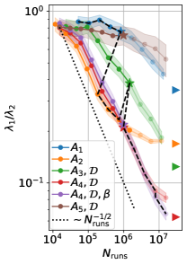
(a)

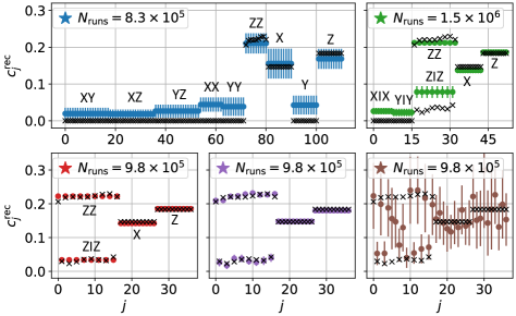
(b)

Figure 2: Hamiltonian learning in presence of weak dissipation. (a) The learning error $\lambda_{1}/\lambda_{2}$ as a function of the number of runs, $N_{\rm runs}$, of the simulator for different ansätze described in the main text. The colored triangles indicate the asymptotic values for $N_{\rm runs}\to\infty$. (b) Snapshots of the (normalized) reconstructed Hamiltonian parameters for some of the ansätze described in the main text. The point at which these snapshots are taken in terms of $N_{\mathrm{runs}}$ is also indicated by asterisks in the left panel. All error bars are computed via bootstrapping as explained in Appendix C, using $80$ samples. Model parameters: The Hamiltonian parameters in Eq. (21) are chosen as $B_{x}=4/5B_{z}$. Moreover, the coupling strengths are described by $4$-th order polynomials of the form $J_{i,i+1}^{z}=B_{z}\sum_{l=1}^{5}a_{l}\cdot x_{i,i+1}^{l-1}$, and $J_{i,i+2}^{z}=B_{z}\sum_{l=1}^{5}b_{l}\cdot x_{i,i+2}^{l-1}$ where $x_{i,j}=[(i+j)-(N+1)]/N$. We choose the following coefficients: $\bm{a}=(6/5,1/20,1/5,0,-2/5)$ and $\bm{b}=(1/5,1/20,-2/5,0,4/5)$. The dissipation rates are chosen such that $(\gamma_{+},\gamma_{-},\gamma_{z})=(1,1.5,2)\times 10^{-2}B^{z}\ll\|H\|$. To estimate the integrals in Eq. (8), we use $B_{z}\Delta_{t}=1/64$, i.e., $64$ equidistant times, where at each time we spend only $1/64$ of the measurements per basis, compared to the quench times $B_{z}T\in[0,0.5,1]$.

In the following, our goal will be to learn the above-described model Hamiltonian and Liouvillian from simulated quench experiments. We will limit the total number of simulated runs $N_{\mathrm{runs}}\approx 10^{6}$, which is a reasonable limit for experiments with trapped ions. We will illustrate how $\bm{c}^{\rm rec}$, including its error bars that we obtain via bootstrapping, and the learning error $\lambda_{1}/\lambda_{2}$ can be used in this scenario to identify the operator content and relevant parameters of the model Hamiltonian and Liouvillian.

III.1.1 Identifying the dominant terms of the Hamiltonian

In a first step, we seek to identify the dominant terms in the Hamiltonian $H$, assuming (prior knowledge) that dissipation is typically weak compared to the Hamiltonian. Therefore, in this first step we will only include an ansatz for the Hamiltonian and no ansatz for the Liouvillian. As, interactions are typically finite range, we generically expect the dominant terms to be nearest-neighbor terms. Moreover, in quantum simulation of condensed matter models one expects more or less homogeneous couplings (translational invariance). Therefore, we start with the following ansatz for the Hamiltonian

$$A_{1}=c_{xx}\sum_{k=1}^{N-1}\sigma_{k}^{x}\sigma_{k+1}^{x}+c_{xy}\sum_{k=1}^{N-1}(\sigma_{k}^{x}\sigma_{k+1}^{y}+\sigma_{k}^{y}\sigma_{k+1}^{x})\\ +\dots+c_{x}\sum_{k=1}^{N}\sigma_{k}^{x}+c_{y}\sum_{k=1}^{N}\sigma_{k}^{y}+c_{z}\sum_{k=1}^{N}\sigma_{k}^{z},$$ (22)

comprising all nearest-neighbor interactions, i.e., $\quantity{xx,yy,zz,xy,xz,yz}$, with spatially homogeneous coefficients. As commuting operators can be measured jointly, the operators in $A_{1}$ can be measured by classically post-processing data obtained from measuring the following nine product operators, independently of the system size: $\sigma_{x}^{\otimes N}$, $\sigma_{y}^{\otimes N}$, $\sigma_{z}^{\otimes N}$, and six operators of the form $\sigma_{a}\otimes\sigma_{b}\otimes\sigma_{a}\otimes\sigma_{b}\otimes\cdots$, for all combinations $a\neq b$ of distinct Pauli operators.

In Fig. 2a we plot $\lambda_{1}/\lambda_{2}$ for the ansatz $A_{1}$ as function of $N_{\mathrm{runs}}$ (blue line). At small $N_{\mathrm{runs}}$ one expects to observe a decrease of $\lambda_{1}/\lambda_{2}$ with $N_{\mathrm{runs}}$ indicating the errors are dominated by shot noise. As the ansatz $A_{1}$ is insufficient, i.e., misses terms present in Eq. (II.1), one expects a plateau in $\lambda_{1}/\lambda_{2}$ for large $N_{\rm runs}$. This plateau appears beyond our maximum measurement budget at $N_{\rm runs}\approx 10^{7}$ experimental runs, which is indicated by a blue triangle on the y-axis in Fig. 2a. Nevertheless, at $N_{\mathrm{runs}}\approx 10^{6}$ the reconstructed parameters $\bm{c}^{\rm rec}$ in Fig. 2b (blue data) identify the dominant terms in the Hamiltonian, i.e., nearest-neighbor $\sigma_{z}\otimes\sigma_{z}$ interactions and fields in $\sigma_{x}$ and $\sigma_{z}$ direction.

At this point, we cannot rule out the presence of the other terms in the operator ansatz $A_{1}$. However, as the values of the non-dominant terms are much smaller than the ones of the dominant terms (see Fig. 2b, blue data), we remove all non-dominant terms from the ansatz in the next step. It should be noted that, in case those terms were present in the Hamiltonian, we would encounter a plateau in $\lambda_{1}/\lambda_{2}$ at a later stage of the learning process. We will later see that this is, however, not the case (as dissipative terms are still missing in our ansatz). On the other hand, if the dominant terms identified from $\bm{c}^{\mathrm{rec}}$ of $A_{1}$ constitute a good approximation to the Hamiltonian, we expect $\lambda_{1}/\lambda_{2}$ to decrease. This is indeed the case as the reparametrized ansatz,

$$\begin{split}A_{2}=c_{zz}\sum_{k=1}^{N-1}\sigma_{k}^{z}\sigma_{k+1}^{z}+c_{x}\sum_{k=1}^{N}\sigma_{k}^{x}+c_{z}\sum_{k=1}^{N}\sigma_{k}^{z}\end{split}$$ (23)

leads to a much smaller value of $\lambda_{1}/\lambda_{2}$. We emphasize that learning with the ansatz $A_{2}$ only requires measurements of $\sigma_{x}^{\otimes N}$ and $\sigma_{z}^{\otimes N}$. Therefore, some of the measurements performed for $A_{1}$ can be recycled for learning the parameters of $A_{2}$. As shown in Fig. 2a (orange line), $A_{2}$ leads to a plateau of $\lambda_{1}/\lambda_{2}$ beginning at $N_{\mathrm{runs}}\approx 3\times 10^{5}$. At this point we have identified all the dominant terms in $H$. To continue the learning process we need to extend the operator ansatz. Therefore, in the next step we want to learn subdominant terms of $H$, as well as the Liouvillian.

III.1.2 Learning the sub-dominant terms of the Hamiltonian, and learning the Liouvillian

One expects, a priori, that when learning smaller terms of the Hamiltonian, weak dissipative effects become relevant. Therefore, we now include an ansatz for the Liouvillian

$$\mathcal{D}(\varrho)=\sum_{\eta\in\{+,-,z\}}\frac{d_{\eta}}{2}\sum_{k=1}^{N}\quantity([\sigma_{k}^{\eta}\varrho,\sigma_{k}^{\eta,\dagger}]+\mathrm{h.c.}),$$ (24)

and extend our ansatz for the Hamiltonian by next-nearest neighbor couplings. As before, we choose our ansatz to be spatially homogeneous, which leads to

$$A_{3}=A_{2}+c_{x1x}\sum_{k=1}^{N-2}\sigma_{k}^{x}\sigma_{k+2}^{x}\\ +c_{y1y}\sum_{k=1}^{N-2}\sigma_{k}^{y}\sigma_{k+2}^{y}+c_{z1z}\sum_{k=1}^{N-2}\sigma_{k}^{z}\sigma_{k+2}^{z}.$$ (25)

This ansatz for the Hamiltonian and Liouvillian requires measurements of the form $\sigma_{x}^{\otimes N}$, $\sigma_{y}^{\otimes N}$ and $\sigma_{z}^{\otimes N}$, which means that all of the data taken for $A_{2}$ can be reused for learning the parameters of $A_{3}$. Note that including dissipation requires the same measurement bases, but at various times to estimate the integrals in Eq. (8).

An ansatz for the dissipation and next-nearest-neighbor terms now leads to a lower plateau of $\lambda_{1}/\lambda_{2}$ compared to $A_{2}$. However, this plateau appears for $N_{\rm runs}\geq 10^{7}$, see Fig. 2a (green line), which exceeds our assumed measurement budget. Nevertheless, the reconstructed parameters of the Hamiltonian, $\bm{c}^{\rm rec}$, at $N_{\rm runs}\approx 10^{6}$, suggest that the next-nearest-neighbor $\sigma_{z}\otimes\sigma_{z}$ couplings are larger compared to other next-nearest-neighbor terms, see Fig. 2b (green data). Therefore, we reparametrize our ansatz for the Hamiltonian to

$$A_{4}=A_{2}+c_{z1z}\sum_{k=1}^{N-2}\sigma_{k}^{z}\sigma_{k+2}^{z}.$$ (26)

Indeed, this leads to a significantly smaller ratio $\lambda_{1}/\lambda_{2}$ compared to $A_{2}$ and $A_{3}$, see Fig. 2a (red line). Moreover, the small error bars in the reconstructed parameters in Fig. 2b (red data) show that $N_{\mathrm{runs}}=10^{6}$ is already sufficient for learning $A_{4}$. Note that at this point, we have identified all dominant and subdominant terms. However, so far we have not learned a possible spatial structure of the couplings in $H$.

III.1.3 Learning the spatial variations of the couplings

As can be seen in Fig. 2a (red line), the plateau in $A_{4}$ is reached at $N_{\mathrm{runs}}\approx 10^{7}$, which again exceeds our available measurement budget. Therefore, we are not allowed to conclude that ansatz $A_{4}$ is insufficient to describe the Hamiltonian in Eq. (II.1) by only considering the ratio $\lambda_{1}/\lambda_{2}$. However, at this point, one can choose to test other ansätze and compare their corresponding reconstructed parameters, or to see if smaller values of $\lambda_{1}/\lambda_{2}$ are achieved. As one typically expects small spatial variations in the couplings of $H$, and $A_{4}$ was already a good approximation of $H$, we want to test for spatial variations on top of the spatially homogeneous ansatz $A_{4}$. To this end, we simply treat the parametrization of the ansatz $A_{4}$ as a regularization of the cost function as explained in Section II.6. That is, we start with the optimization problem in Eq. (20), and $\beta\gg 1$. This imposes the exact parametrization of $A_{4}$, and we then successively decrease $\beta$ until one observes the emergence of spatial variations, and the corresponding error bars, see Fig. 2b (violet data). This ensures that our learning process is dominantly limited by shot noise, and not by having too few parameters in the ansatz.

With a larger measurement budget one could then successively increase $N_{\mathrm{runs}}$ while decreasing $\beta$, until the desired accuracy is reached, which is reminiscent of Bayesian learning [30, 39]. Therefore, we conclude that we have indeed successfully determined the operator content and parameters of the Hamiltonian and Liouvillian in our simulated experiment.

As a final step, we may compare the reconstructed parameters of our learning procedure to the ones obtained from a "naive" ansatz of the form

$$A_{5}=\sum_{k=1}^{N-1}c_{zz}^{(k)}\sigma_{k}^{z}\sigma_{k+1}^{z}+\sum_{k=1}^{N-2}c_{z1z}^{(k)}\sigma_{k}^{z}\sigma_{k+2}^{z}\\ \qquad+\sum_{k=1}^{N}c_{x}^{(k)}\sigma_{k}^{x}+\sum_{k=1}^{N}c_{z}^{(k)}\sigma_{k}^{z},$$ (27)

that has a total of $4N-3$ parameters. One notices that our strategy leads to a much more accurate reconstruction, cf. Fig. 2b (brown data).

III.2 Liouvillian Learning of a long-range interacting many-body system

In this section, we illustrate Liouvillian learning for a model system involving long-range spin-spin interactions, as realized in trapped-ion setups. The effective Hamiltonian is given by [9]

$$\begin{split}H_{\mathrm{XY}}=\sum_{i<j}^{N}J_{ij}\left(\sigma_{i}^{x}\sigma_{j}^{x}+\sigma_{i}^{y}\sigma_{j}^{y}\right)+\sum_{i=1}^{N}B_{i}\sigma_{i}^{z},\end{split}$$ (28)

with interaction strengths $J_{ij}$ and site-dependent magnetic field $B_{i}$. In an idealized description, it is often assumed that

$$\begin{split}J_{ij}=\frac{J_{0}}{|p(i)-p(j)|^{\alpha}},\quad B_{i}=B_{z},\end{split}$$ (29)

where $p(i)$ is the position of the $i$-th ion and with tunable $0\leq\alpha\leq 3$. To add features to the model, we assume that the ions are randomly shifted from their equilibrium positions, i.e., $p(i)=i+r_{i}$, where each $r_{i}$ is sampled uniformly from $[-0.05,0.05]$. Models with random ion positions are studied, for example, in the context of topological defects in the Frenkel-Kontorova model [49, 50].

To account for spontaneous emission of trapped ions, we add the spatially homogeneous Lindblad terms

$$\mathcal{L}_{D}^{-}(\varrho)=\frac{\gamma^{-}}{2}\sum_{k=1}^{N}\left([\sigma_{k}^{-}\varrho,\sigma_{k}^{-,\dagger}]+[\sigma_{k}^{-},\varrho\sigma_{k}^{-,\dagger}]\right).$$ (30)

Moreover, we assume the presence of dephasing terms originating from the presence of a fluctuating, classical magnetic field, that leads to shifts of the energy levels of the $k$-th ion proportional to $B_{k}^{\mathrm{cl}}(t)$. It can be shown that in the white-noise limit, i.e., with correlation function $\langle B_{k}^{\mathrm{cl}}(t)B_{l}^{\mathrm{cl}}(t^{\prime})\rangle=\Gamma_{kl}^{z}\delta(t-t^{\prime})$, this leads to Lindblad terms of the form

$$\begin{split}\mathcal{L}_{D}^{z}(\varrho)=\sum_{k,l=1}^{N}\Gamma_{kl}^{z}\Big{\{}\sigma_{k}^{z}\varrho\sigma_{l}^{z}-\frac{1}{2}(\sigma_{k}^{z}\sigma_{j}^{z}\varrho+\varrho\sigma_{k}^{z}\sigma_{j}^{z})\Big{\}}.\end{split}$$ (31)

In particular, uncorrelated magnetic field fluctuations lead to a diagonal matrix $\Gamma_{kl}^{z}=\gamma_{k}^{z}\delta_{kl}$, whereas global fluctuations, with $B_{k}^{\mathrm{cl}}(t)=B^{\mathrm{cl}}(t)$ for all $k$, lead to a constant matrix $\Gamma_{kl}^{z}=\Gamma_{0}$. In the present example we will, for simplicity, only consider uncorrelated and global fluctuations, which lead to a matrix

$$\Gamma_{kl}^{z}=\gamma_{k}^{z}\delta_{kl}+\Gamma_{0},$$ (32)

[see also Fig. 3 for the specific choices of parameters]. We note, that in experiments with, for instance, long ion strings, or local magnetic fields one expects a more complicated structure of the matrix $\Gamma_{kl}^{z}$.

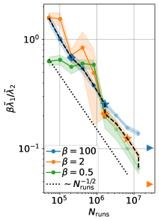
(a)

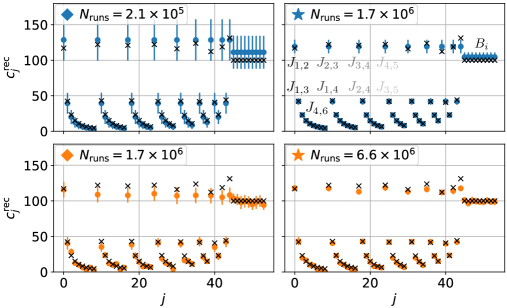
(b)

Figure 3: Hamiltonian learning in presence of collective dissipation. (a) The ratio $\tilde{\lambda}_{1}/\tilde{\lambda}_{2}$ after excluding the conserved quantity $Q$ for different regularization parameters $\beta$. The colored triangles describe the asymptotic values at $N_{\mathrm{runs}}\to\infty$. (b) Snapshots of the learned Hamiltonian parameters as indicated by the asterisks in the left panel. All error bars are computed via bootstrapping as explained in Appendix C, using $10$ samples. The integrals in Eq. (8) are evaluated using $B_{z}\Delta_{T}=1/128$, i.e., using $128$ time-steps, where at each time we use only a fraction of $1/128$ number of measurements per basis, compared to the quench times $B_{z}T\in[0,0.5,1]$. The auxiliary parameter $\xi$ for the additional constraints as introduced in Eq. (11) is set to $\xi=1000$. Model parameters: For the Hamiltonian we choose parameters as specified in Eq. (29) with $B_{z}=100$, $J_{0}=6/5B_{z}$ and $\alpha=1.5$. Moreover, in the Liouvillian, we choose $\gamma_{-}=B_{z}/20$ in Eq. (30), as well as $\Gamma_{kl}^{z}=\gamma_{k}^{z}\delta_{kl}+\Gamma_{0}$ with $\Gamma_{0}=B_{z}/40$ and $\gamma_{k}^{z}=3\Gamma_{0}$ in Eq. (31).

III.2.1 Ansatz for learning $H_{\mathrm{XY}}$

In Section III.1, we have already illustrated our strategy for learning the operator content, as well as the relevant parameters of the Hamiltonian from minimal prior knowledge. Therefore, we start here with a parametrized ansatz, that already incorporates the algebraically decaying spin-spin interactions in $H_{\mathrm{XY}}$, that one would expect to find in a trapped-ion experiment, as well as a constant magnetic field. We choose as an ansatz for the Hamiltonian

$$A(c_{0},\alpha,b)=\sum_{i<j}\frac{c_{0}}{|i-j|^{\alpha}}(\sigma_{i}^{x}\sigma_{j}^{x}+\sigma_{i}^{y}\sigma_{j}^{y})+b\sum_{k}\sigma_{k}^{z},$$ (33)

which depends non-linearly on the parameter $\alpha$, and hence, will require non-linear minimization of $\lambda_{1}$ over $\alpha$.

As we also want to learn the dissipative processes, we will start with an ansatz for the Liouvillian, comprising single-qubit Lindblad operators that typically appear in the context of trapped-ion experiments, i.e.,

$$\mathcal{D}^{\mathrm{loc}}(\varrho)=\sum_{\eta\in\{+,-,z\}}\frac{d_{\eta}}{2}\sum_{k=1}^{N}\quantity([\sigma_{k}^{\eta}\varrho,\sigma_{k}^{\eta,\dagger}]+\mathrm{h.c.}),$$ (34)

Note that this ansatz does not include collective dissipation as given by the off-diagonal elements of $\Gamma^{z}_{kl}$ in the model Liouvillian. Nevertheless, we will find, that the ansatz in Eq. (34) is sufficient for learning the Hamiltonian, and we will discuss in detail why this is the case.

III.2.2 Learning a disordered Hamiltonian

Let us now illustrate learning of the long-range Hamiltonian $H_{\mathrm{XY}}$ using the physically motivated ansätze in Eqs. (33) and (34). Firstly, one notices that the ansatz $A$ contains the total magnetization defined by

$$Q=B\sum_{k}\sigma^{z}_{k},$$ (35)

which commutes with $H_{XY}$ for any $B\in\mathbb{R}$. Therefore, $Q$ is a conserved quantity of $\mathcal{L}_{H}$. This leads to a degeneracy of the singular value spectrum of the constraint matrix $M(\bm{d})$, i.e., we observe, that $\lambda_{1}\approx\lambda_{2}$. In particular, this means that the reconstructed parameters $\bm{c}^{\rm rec}$ will be a linear combination of the parameters of $H_{\mathrm{XY}}$ and $Q$. To reconstruct the parameters of the Hamiltonian, including its overall-scale, we need to exclude $Q$, as well as scalar multiples of the Hamiltonian, $\nu\cdot H_{\mathrm{XY}}$, as possible solutions for $\bm{c}^{\mathrm{rec}}$. This is achieved by imposing additional constraints as discussed in Section II.3. To this end, we choose a set of operators, $\mathcal{O}=\{\sigma_{1}^{x},\sigma_{1}^{y},\sigma_{1}^{z}\}$, where some operators do not commute with $Q$, while others do not commute with $H_{\mathrm{XY}}$. Here, one could in principle also choose random operators. This leads to a combined linear optimization as in Eq. (11) [see also Appendix A for the detailed structure of the additional constraints]. Moreover, one can define a projected constraint matrix with non-degenerate spectrum $\tilde{\lambda}_{1}\leq\tilde{\lambda}_{2}\leq\dots$, where $\bm{c}^{\rm rec}\approx\bm{c}^{H}$ is the right-singular vector corresponding to $\tilde{\lambda}_{1}$. Then, $\tilde{\lambda}_{1}/\tilde{\lambda}_{2}$ becomes the analog of $\lambda_{1}/\lambda_{2}$ .

In Fig. 3a we monitor $\tilde{\lambda}_{1}/\tilde{\lambda}_{2}$ as a function of $N_{\mathrm{runs}}$ for the ansatz $A_{XY}$, and for different values of the regularization parameter $\beta$. One starts with a large value of the regularization parameter, here, $\beta=100$, which strongly imposes the parametrization of $A_{XY}$, leading to reconstructed parameters without spatial disorder, see Fig. 3b for $N_{\mathrm{runs}}=2.1\times 10^{5}$ (blue data). Then further increasing $N_{\mathrm{runs}}$ reduces the size of the error bars in $\bm{c}^{\mathrm{rec}}$, as is also shown in Fig. 3b for $N_{\mathrm{runs}}=1.7\times 10^{6}$ (blue data). However, an ansatz with $\beta=100$ cannot account for disorder in the coupling terms in $H_{XY}$, which is shown by the plateau in $\tilde{\lambda}_{1}/\tilde{\lambda}_{2}$, here, starting at around $N_{\mathrm{runs}}\approx 10^{7}$ (blue line), which, again, is above our measurement budget. Nevertheless, we decrease the regularization parameter $\beta$, which leads to larger error bars, but also allows to learn some of the spatial disorder in $H_{\mathrm{XY}}$, as is shown in Fig. 3b for $\beta=2$ and $N_{\mathrm{runs}}=1.7\times 10^{6}$ (orange data). Note that already before reaching a plateau for $\beta=2$ in Fig. 3a (orange line) the error bars of $\bm{c}^{\mathrm{rec}}$ become very small, which can be seen in Fig. 3b for $\beta=2$ and $N_{\mathrm{runs}}=6.6\times 10^{6}$ (orange data). This suggest to further reduce $\beta$. Ultimately, this process of subsequently reducing $\beta$ and increasing $N_{\mathrm{runs}}$ allows us to learn $H_{\mathrm{XY}}$ up to statistical errors, and leads to $\tilde{\lambda}_{1}/\tilde{\lambda}_{2}\sim N_{\mathrm{runs}}^{-1/2}$ for the entire range of $N_{\mathrm{runs}}$.

So far we have used an ansatz for the Liouvillian which does not include the collective dephasing terms in Eq. (31). Nevertheless, we can learn the Hamiltonian to a high accuracy, which constitutes a useful feature of our approach. To see why this is the case, we evaluate the matrix $M_{D}(\bm{d})$ by summing Eq. (8) over all Lindblad operators, yielding

$$[M_{D}(\bm{d})]_{\kappa,(i,j)}=\sum_{k,l}d_{kl}[M^{(k,l)}]_{\xi,(i,j)}\\ =\int_{0}^{T}\sum_{k,l}d_{kl}\expectationvalue*{\sigma_{k}^{z}[h_{ij},\sigma_{l}^{z}]+\mathrm{h.c.}}_{\kappa,t}\mathrm{d}t,$$ (36)

where $\kappa$ labels input states. Here, we only include the interaction terms, $h_{ij}=\sigma_{i}^{x}\sigma_{j}^{x}+\sigma_{i}^{y}\sigma_{j}^{y}$, of the Hamiltonian $H_{XY}$, since the contribution of the collective dissipation in Eq. (31) vanishes for the field terms $\sigma_{i}^{z}$. Considering the sum over operators appearing in the expectation value in Eq. (36), we can split this sum into

$$\sum_{k=1}^{N}d_{kk}\Big{(}\sigma_{k}^{z}[h_{ij},\sigma_{k}^{z}]+\mathrm{h.c.}\Big{)}+\sum_{k\neq l}^{N}d_{kl}\Big{(}\sigma_{k}^{z}[h_{ij},\sigma_{l}^{z}]+\mathrm{h.c.}\Big{)}\\ =-4\sum_{k=1}^{N}d_{kk}(\delta_{ki}+\delta_{kj})h_{ij}+4\sum_{k\neq l}^{N}d_{kl}(\delta_{ki}\delta_{lj}+\delta_{kj}\delta_{li})h_{ij},$$

which vanishes for $d_{kl}=d_{0}$. Therefore, the constraint matrix in Eq. (7) and hence also the reconstructed parameters of the Hamiltonian are not affected by including collective dissipation into our ansatz. However, this will change if we include additional constraints, as we demonstrate in the following.

III.2.3 Learning collective dissipation

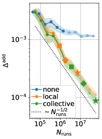
(a)

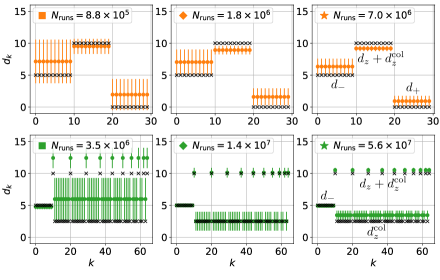
(b)

Figure 4: Learning collective dissipation using the additional constraints defined in the main text, and regularization strength $\beta=2$. (a) The error of the additional constraints $\Delta^{\mathrm{add}}$ as introduced in Eq. (38) for different ansätze for the dissipation as described the main text. (b) Snapshots of the learned dissipation rates $d_{k}^{\mathrm{rec}}$ as marked by the asterisks in the left panel. All error bars are computed via Bootstrapping as explained in Appendix C, using $10$ samples. Integrals for dissipation correction are evaluated as for Fig. 3.We further restrict $d_{-},d_{z},d_{z}^{\mathrm{col}}\geq 0$ and numerically search for the optimal rates within the bounds.

To discover the collective dissipation given by Eq. (31) we choose the following ansatz for the Liouvillian

$$\mathcal{D}^{\mathrm{col}}(\varrho) =\frac{d_{-}}{2}\sum_{k=1}^{N}\quantity([\sigma_{k}^{-}\varrho,\sigma_{k}^{-,\dagger}]+\mathrm{h.c.})$$ (37)

$$+\sum_{k,l=1}^{N}(d_{z}\delta_{kl}+d_{z}^{\rm col}(1-\delta_{kl}))\mathcal{D}^{z}_{kl}(\varrho),$$

that includes single-qubit spontaneous decay with jump operator $\sigma_{k}^{-}$, and single-qubit as well as collective dephasing $\mathcal{D}^{z}_{kl}$ with operator structure as described in Eq. (31). Learning collective dissipation requires the set of constraint operators to also include two-qubit terms. This is because single-qubit operators are not affected by the multi-qubit Lindblad operators in Eq. (31). Therefore, we may choose the following set of constraint operators

$$\mathcal{O}=\{\sigma_{1}^{x},\sigma_{1}^{y},\sigma_{1}^{z},\sigma_{2}^{x},\sigma_{2}^{y},\sigma_{2}^{z},\sigma_{1}^{x}\sigma_{2}^{x},\sigma_{1}^{x}\sigma_{2}^{y},\sigma_{1}^{y}\sigma_{2}^{x},\sigma_{1}^{y}\sigma_{2}^{y}\}.$$

Note that we included here the local operators despite the fact that they cannot help to learn the collective dissipation. This is due to the facts that their expectation values can be obtained from post-processing the data obtained from measuring the two-body operators and that they can be used to better learn the overall scale and the local dissipation rates, as discussed above. Let us emphasize, that the ratio $\lambda_{1}/\lambda_{2}$ is not affected by taking collective dissipation in the ansatz into account. Therefore, we instead use

$$\Delta^{\mathrm{add}}\vcentcolon=\|M^{\mathrm{add}}\bm{c}^{\mathrm{rec}}-\bm{b}(\bm{d}^{\mathrm{rec}})\|,$$ (38)

as a measure of how well the additional constraints are fulfilled. In case an ansatz for the Liouvillian is insufficient, not any possible additional constraint can be exactly fulfilled. In such a case, $\Delta^{\mathrm{add}}$ will be bounded away from zero in the limit $N_{\rm runs}\to\infty$. However, in practice, with only a few additional constraints, e.g., the local Pauli operators discussed above, this must not be the case.

In Fig. 4a we monitor $\Delta^{\mathrm{add}}$ as a function of $N_{\mathrm{runs}}$ for the Hamiltonian ansatz in Eq. (33) with $\beta=2$, for different ansätze for the Liouvillian. For an ansatz that does not include dissipation (blue line in Fig. 4a) we observe a plateau of $\Delta^{\mathrm{add}}$ already at very early stages of the learning procedure, here at $N_{\rm runs}\approx 10^{5}$. On the other hand, we find that the ansätze containing local (orange line) and collective (green line) dissipation lead to similar values of $\Delta^{\mathrm{add}}$ in early states of the learning procedure. Only above $N_{\mathrm{runs}}\approx 10^{7}$ the insufficiency of the local ansatz Eq. (34) would become evident from considering $\Delta^{\mathrm{add}}$, which is beyond our available measurement budget. Nevertheless, we can study the reconstructed parameters shown in Fig. 4b and their corresponding error bars. For the ansatz with local dissipation (orange data) we find that the learned rates converge to the exact values, with a good reconstruction achieved at around $N_{\mathrm{runs}}\approx 10^{6}$. Note that here the learned dephasing rate is the sum $d_{z}+d_{z}^{\mathrm{col}}$. For the ansatz including collective dissipation (green data) we obtain similarly accurate values for $\gamma_{-}$. However, the local and global dephasing rates, $d_{z}$ and $d_{z}^{\mathrm{col}}$ respectively, have larger error bars. Only around $N_{\mathrm{runs}}\approx 10^{7}$ we observe the emergence of non-zero dissipation rates for collective dephasing. This concludes the learning procedure of the Hamiltonian and Liouvillian.

IV Conclusion and Outlook

In this study, we have devised a method for learning Hamiltonian and Liouvillian in the analog quantum simulation of many-body systems. Our work applies to a scenario where one has direct access to the quantum device, however, in the literature, other scenarios have been considered, where one does not have direct access to the quantum device, see, e.g., Refs. [25, 52]. Our method is applicable in a regime of experimental relevance where the dissipation is weak compared to the coherent evolution. Our protocol is based on quench experiments, where initial product states evolve under coherent and dissipative dynamics, and the resulting state is measured in a product basis. Hamiltonian and Liouvillian learning can be understood as a sample efficient process tomography of quantum simulators. The learning method begins with an ansatz for the operator structure of the Hamiltonian and Liouvillian. The quality of this ansatz can be monitored by measuring the learning error. Our strategy encompasses the reparametrization of the ansatz. This typically allows data recycling from previous measurement runs, but requires additional classical post-processing. This approach enables us to identify step by step first the dominant operator content of the Hamiltonian and Liouvillian, and successively sub-dominant terms within a limited measurement budget. A distinctive feature of our approach is that we can learn the Hamiltonian without the necessity to learn the entire Liouvillian, thus reducing the number of parameters to be learned. However, we demonstrated that additional constraints can be employed to learn the entire Liouvillian and to ascertain the overall scale of the Hamiltonian. Furthermore, these additional constraints can facilitate the learning of the Hamiltonian even when there are conserved quantities as operators commuting with the system Hamiltonian. While the focus of the present paper has been on spin models, the central ideas of Hamiltonian and Liouvillian learning also carry over to Bose and Fermi Hubbard models.

Extensions of the present work should consider scenarios where the experimental Hamiltonian (and Liouvillian) involves a large number of small terms, which, e.g., emerge as corrections in effective many-body spin models in a low-energy description. Such a formulation might involve a statistical description as learning of an ensemble of Hamiltonians. Along similar lines, Hamiltonian learning might also account for slow drifts of experimental Hamiltonians and Liouvillians. Considering alternative viewpoints, Hamiltonian and Liouvillian learning can also be phrased in the language of Bayesian inference, similar to Ref. [30], establishing an interesting link between techniques of parameter estimation in multi-parameter quantum metrology, and optimal sensing with finite measurement budgets. Finally, exploring alternative routes should include shadow-tomography tomography [53] to estimate expectation values of many few-body observables, relevant in cases where the Hamiltonian consists of many non-commuting terms, and using (short-range) entangled states as inputs, which may be easily prepared in experiments.

Appendix A Additional constraints

As we have already pointed out in the main text, Eq. (7) alone is not sufficient for learning the Hamiltonian, as $H$ is only determined up to an overall scale, and, possibly, conserved quantities not proportional to $H$. Moreover, it may happen that the dissipation rates are not uniquely determined, even in case the ansatz for the dissipation is correct. These ambiguities result from invariances of the conditions in Eq. (7), some of which we have already discussed in the main text. In the following, we show that by including additional constraints Eq. (7) can become sufficient for learning $H$, including its overall scale, and to learn the Liouvillian.

As explained in the main text, the idea is to impose additional constraints to single out the vector $\bm{c}^{H}$ of $H$ (or the vector $\bm{d}^{\mathcal{L}}$ of dissipation rates of $\mathcal{L}_{D}$) as the unique solution to Eq. (9). To this end, we consider the equation of motion of a general observable, $O$, not commuting with $H$, which is given by the Ehrenfest theorem, i.e.,

$$\frac{\mathrm{d}}{\mathrm{d}t}\expectationvalue*{O}=\expectationvalue{-i[O,H]}\\ +\frac{1}{2}\sum_{k}\gamma_{k}\langle l_{k}^{\dagger}[O,l_{k}]+[l_{k}^{\dagger},O]l_{k}\rangle.$$ (39)

Instead of choosing $O=H$, as we did below Eq. (3) to obtain the constraints in $M(\bm{d})$, we now have to insert the ansätze $A(\bm{c})$ for $H$ and $\Gamma(\bm{d})$ for the dissipative terms. Thus, after taking the integral from $t=0$ to $t=T$, we obtain a set of linear equations for $\bm{c}$ and $\bm{d}$. Again, these can be written as a simple matrix equation;

$$M^{\mathrm{add}}\bm{c}=\bm{b}(\bm{d}),$$ (40)

where

$$M^{\mathrm{add}}_{ij}=\int_{0}^{T}\expectationvalue*{-\mathrm{i}[O,h_{j}]}_{i,t}\mathrm{d}t,$$ (41)

and

$$b_{i}(\bm{d})=\expectationvalue*{O}_{i,T}-\expectationvalue*{O}_{i,0}\\ -\frac{1}{2}\sum_{k}d_{k}\int_{0}^{T}\expectationvalue*{a_{k}^{\dagger}[O,a_{k}]+\mathrm{h.c.}}_{i,t}\,\mathrm{d}t.$$ (42)

Note, that similar constraints have also been used in Ref. [32] to learn Liouvillians from their steady-states. Compared to the conditions in Eq. (7), the constraints above contain additional integrals in Eq. (41) that need to be estimated from experimental data. To obtain the reconstructed parameters we solve the combined system of equations including the additional constraints, i.e.,

$$\bm{c}_{0}^{\mathrm{rec}}(\xi)=\\ \underset{\bm{c}}{\mathrm{arg}\,\mathrm{min}}\left[\min_{\bm{d}\geq 0}\Big{\|}\begin{pmatrix}M(\bm{d})\\ \xi M^{\mathrm{add}}\end{pmatrix}\bm{c}-\begin{pmatrix}0\\ \xi\bm{b}(\bm{d})\end{pmatrix}\Big{\|}\right],$$ (43)

where the parameter $\xi$ controls the relative weight between the constraints defined by $M(\bm{d})$ and $M^{\mathrm{add}}$. In analogy to Eq. (9), solving Eq. (43) requires a simultaneous minimization over $\bm{c}$ and $\bm{d}$, while $\xi$ serves as a ’hyper-parameter’ of the optimization. For $\xi=0$ the vector $\bm{c}_{0}^{\mathrm{rec}}(0)$ may be a linear combination of the Hamiltonian and additional, linearly independent, conserved quantities due to the degeneracy of the spectrum of $M(\bm{d})$, as discussed in the main text. Then, by choosing the value of $\xi$ large enough, one removes components of conserved quantities from $\bm{c}_{0}^{\mathrm{rec}}$. In a similar way, one can choose additional constraints such that the solution for the dissipation rates $\bm{d}$ becomes unique.

Note that the norm of $\bm{c}_{0}^{\mathrm{rec}}$ in Eq. (43) depends on $\xi$ and becomes exact only in the limit $\xi\to\infty$. A finite $\xi$ typically leads to a smaller value for the overall scale of the Hamiltonian. This is because the homogeneous part of Eq. (43) is perfectly solved for $\bm{c}=0$. Nevertheless, one obtains a $\bm{c}^{\mathrm{rec}}_{0}\propto\bm{c}^{H}$. Then, the correct overall scale $s$, defined by $\bm{c}^{H}=s\cdot\bm{c}^{\mathrm{rec}}_{0}$, can be determined solely via the additional constraints

$$\sum_{j}M^{\mathrm{add}}_{ij}(s\bm{c}_{0}^{\mathrm{rec}})_{j}=b_{i}(\bm{d}^{\rm rec}).$$ (44)

where $\bm{d}^{\mathrm{rec}}$ are the optimal dissipation rates determined from Eq. (43). Then, averaging over all additional constraints

$$s=\frac{1}{p}\sum_{i=1}^{p}\frac{b_{i}(\bm{d}^{\mathrm{rec}})}{(M^{\mathrm{add}}\bm{c}_{0}^{\mathrm{rec}})_{i}}$$ (45)

yields the correct overall scale.

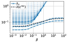
(a)

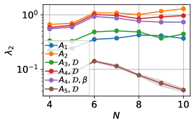
(b)

Figure 5: (a) Singular value spectrum of $M_{G}(\beta)$ defined in Eq. (51) as a function of the regularization strength $\beta$ for the model introduced in Section III.2 in the main text. Increasing $\beta$ opens a gap between the image of the parametrization matrix $G$ introduced in Appendix B and the rest of the spectrum. Within this subspace, $\lambda(\bm{c}^{\mathrm{rec}})$, defined in Eq. (52), follows the best approximation to the Hamiltonian of the system. (b) Scaling of the second-lowest singular value $\lambda_{2}$ with system size $N$, for the same model and ansätze as in Section III.1 and fixed $N_{\mathrm{runs}}=3.1\times 10^{7}$. One finds that $\lambda_{2}$ does not decrease with system size if the number of free parameters in the ansatz is kept constant, which is the case for all ansätze except $A_{5}$.

Appendix B (Re-)Parameterization

As we have seen in the main text, ansatz reparamtetrization is one of the central tools used in the strategy we have devised. Therefore, we want to discuss here in more detail the different possibilities to reparametrize an ansatz. In general, there are two different strategies but we will show that both can be understood in terms of regularization of the cost function in Eq. (9).

In the first reparametrization strategy the vector of parameters, $\bm{c}$, is mapped via a parametrization matrix $G$ to a new vector of parameters, $\bm{c}_{G}=G^{T}\bm{c}$. Here, the matrix $G$ is a $n\times\tilde{n}$ matrix, with $n\geq\tilde{n}$, encoding the dependencies between the $n$ parameters in $\bm{c}$, and the $\tilde{n}$ parameters in $\bm{c}_{G}$. Moreover, one requires that $G=(\bm{g}_{1},\dots,\bm{g}_{\tilde{n}})$, with orthonormal columns $\langle\bm{g}_{i}|\bm{g}_{j}\rangle=\delta_{ij}$. One can easily verify that $G^{T}G=\mathds{1}_{\tilde{n}\times\tilde{n}}$, and $GG^{T}=\sum_{i=1}^{\tilde{n}}\outerproduct{\bm{g}_{i}}{\bm{g}_{i}}$, which is a projector onto the support of $G^{T}$, and thus $G$ is an isometry. In particular cases $G$ can also depend on non-linear parameters, i.e.,

$$G=G(\bm{\alpha})=(\bm{g}_{1}(\bm{\alpha}),\dots,\bm{g}_{\tilde{n}}(\bm{\alpha})).$$ (46)

In either case, the new ansatz is given by $A_{G}(\bm{c}_{G})=A(G\bm{c}_{G})$. This also transforms the constraint matrices via

$$M^{\mathrm{H}}_{G}=M^{\mathrm{H}}G,\quad M^{\mathrm{D}}_{G}(\bm{d})=M^{\mathrm{D}}(\bm{d})G,$$ (47)

where the columns of the new constraint matrices are obtained as linear combinations of the columns of the old constraint matrices. The parametrized reconstructed parameters can be obtained as solutions of

$$\bm{c}^{\mathrm{rec}}_{G}=\underset{\bm{c}_{G},\|\bm{c}_{G}\|=1}{\mathrm{arg}\,\mathrm{min}}\left[\min_{\bm{d}\geq 0}\norm{[M_{G}^{\mathrm{H}}+M_{G}^{\mathrm{D}}(\bm{d})]\bm{c}_{G}}\right],$$ (48)

and similarly for Eq. (43). In the case where $G$ depends on non-linear parameters $\bm{\alpha}$, the above optimization also includes a minimization over $\bm{\alpha}$. Numerically, the optimal $\bm{\alpha}$ can be found similarly to the optimal dissipation rates $\bm{d}^{\mathrm{rec}}$ in Eq. (9), using the DIRECT algorithm in SciPy.

We wish to emphasize that by using this way of parametrizing an ansatz, one obtains reconstructed parameters, where the dependencies, encoded in the matrix $G$, are exactly fulfilled. Examples for such a reparametrization include, for instance, disregarding operators from the operator content of $A(\bm{c})$. This can be understood as a reparametrization, where $(\bm{g}_{i})_{k}=0$, for all $i\in[0,\tilde{n}]$, and $k\in[0,n]$ for which we want to remove the corresponding operator $h_{k}$ from the operator content of $A(\bm{c})$.

Instead of imposing an exact parametrization on an ansatz, one may only impose it approximately. In practice, this may be very useful as parametrizations are almost never exactly fulfilled, but only to a very good approximation. To this end, one adds a penalty term to the cost function in Eq. (9), which acts as a regularizing term, giving preference to solutions approximately admitting a certain parametrization. In case of a parametrization $G$, as defined above, the corresponding optimization problem reads

$$\bm{c}^{\mathrm{rec}}(\beta)=\underset{\bm{c},\|\bm{c}\|=1}{\mathrm{arg}\,\mathrm{min}}\left[\min_{\bm{d}\geq 0}\norm{[M_{\mathrm{H}}+M_{\mathrm{D}}(\bm{d})]\bm{c}}\right.\\ \left.+\beta\norm{(\mathds{1}-GG^{T})\bm{c}}\vphantom{\min_{\bm{d}\geq 0}}\right],$$ (49)

where $\beta\in[0,\infty)$ is the regularization strength. For $\beta=0$ this corresponds to the original unconstrained (i.e., unparametrized) problem in Eq. (9). For non-zero $\beta$ the last term adds a penalty, whenever $\bm{c}$ has a component outside of the range of $GG^{T}$, where the parametrization implied by $G$ is exactly fulfilled. The larger $\beta$, the more $\bm{c}^{\rm rec}$ is constrained by the parametrization $G$. In the limit $\beta\rightarrow\infty$ the parametrization $G$ is fulfilled exactly, and the optimization problem corresponds to the one in Eq. (48). This can be seen as follows; the objective function in Eq. (48) can be rewritten as $\norm{[M_{\mathrm{H}}+M_{\mathrm{D}}(\bm{d})]GG^{T}\bm{c}}$, where the feasible region consists of all $\bm{c}$ for which $\bm{c}=GG^{T}\bm{c}$. This in turn can be written as an unconstrained problem in Eq. (49), where $\beta\rightarrow\infty$. Note, that solving the minimization problem in Eq. (49) is equivalent to solving the linear problem

$$\bm{c}^{\mathrm{rec}}(\beta)=\underset{\bm{c},\|\bm{c}\|=1}{\mathrm{arg}\,\mathrm{min}}\left[\min_{\bm{d}\geq 0}\left\|\begin{pmatrix}M_{\mathrm{H}}+M_{\mathrm{D}}(\bm{d})\\ \beta(\mathds{1}-GG^{T})\end{pmatrix}\bm{c}\right\|\right].$$ (50)

We now want to study the effect of $\beta$ on the singular value spectrum of the matrix

$$M_{G}(\beta)=\begin{pmatrix}M_{\mathrm{H}}+M_{\mathrm{D}}(\bm{d}^{\mathrm{rec}})\\ \beta(\mathds{1}-GG^{T})\end{pmatrix},$$ (51)

for the example in Section III.2 (see Fig. 5a). As expected, in the limit $\beta\to 0$, the spectrum converges to the spectrum of the unparametrized constraint matrix $M(\bm{d}^{\rm rec})$. Here, the gap between the lowest singular values and the rest of the spectrum becomes very small, resulting in an unstable solution. Then, when increasing $\beta$, all singular values, whose corresponding right-singular vectors are incompatible with the regularization increase with $\beta$, opening a gap to the subspace spanned by the regularization, i.e., the image of $G$, which in the case of the ansatz in Eq. (33) is $2$-dimensional. Note, that the Hamiltonian in Eq. (28) only approximately lies in the image of $G$. Therefore, also the lowest singular values initially increase with $\beta$, until they reach a constant value, that corresponds to an exactly enforced parametrization. Along this path, we can monitor the minimum of the cost function in Eq. (50) defined via

$$\lambda(\bm{c}^{\mathrm{rec}})=\left\|\begin{pmatrix}M_{\mathrm{H}}+M_{\mathrm{D}}(\bm{d}^{\mathrm{rec}})\\ \beta(\mathds{1}-GG^{T})\end{pmatrix}\bm{c}^{\mathrm{rec}}\right\|,$$ (52)

which follows the singular value that corresponds to the best approximation of the Hamiltonian. This indicates successful exclusion of the conserved quantity via the additional constraints, as discussed in Section III.2 in the main text.

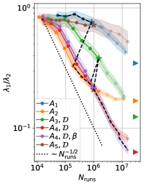
(a)

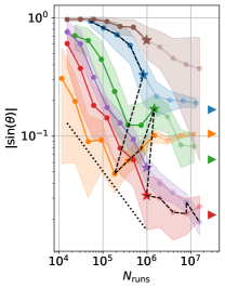
(b)

Figure 6: Comparison of $\lambda_{1}/\lambda_{2}$ (experimentally accessible), and $\sin(\theta)$ (not experimentally accessible), as a function of the number of runs, $N_{\rm runs}$. The different ansätze are defined in Section III.1 in the main text. Error bars are computed via bootstrapping as described in Appendix C, using $80$ samples. The colored triangles indicate the asymptotic values in the limit $N_{\rm runs}\to\infty$. Both quantities show a similar behaviour which supports using $\lambda_{1}/\lambda_{2}$ to asses the quality or learning error of an ansatz.

Appendix C Bootstrapping

To obtain error bars from data we use the Bootstrapping method, which we will introduce below. Assume we are given a single realization $x_{1},\dots,x_{n}$ of a set of independent and identically distributed random variables $X_{1},\dots,X_{n}$ with unknown distribution function. We are interested in estimating the variance of a given function $T(X_{1},\dots,X_{n})$. To do so we draw $n$ times with replacement from $x_{1},\dots,x_{n}$, yielding a sample $x_{1}^{\ast},\dots,x_{n}^{\ast}$, and then evaluate $t=T(x_{1}^{\ast},\dots,x_{n}^{\ast})$. We repeat this procedure $r$ times obtaining $t^{(1)},\dots,t^{(r)}$, and then estimate the variance of $T$ from the sample variance of $t^{(1)},\dots,t^{(r)}$.

In our case the $X_{1},\dots,X_{n}$ are the individual measurements in a given basis for fixed initial state and simulation time. One can also think of $X_{1},\dots,X_{n}$ to be individual measurements of a given observable for fixed initial state and simulation time, in the case where the measurements of different observables are independent. Then the quantities of interest $T(X_{1},\dots,X_{n})$ are, e.g., the learned parameters $\bm{c}^{\mathrm{rec}}$, or the ratio of singular vales $\lambda_{1}/\lambda_{2}$. The number of samples $r$ is chosen the minimum possible integer, such that the error bars do not significantly change anymore when further increasing $r$.

Appendix D Scalability

In the context of Hamiltonian learning it was shown in Ref. [35] that, under the premise that $H$ is a local many-body Hamiltonian, the experimental resources required for Hamiltonian learning scale only polynomially in the system size, and are even constant in system size in the case of a translation invariant Hamiltonian. As we are considering the limit of weakly dissipative dynamics, where the Liouvillian only gives a small perturbation to the coherent time-evolution generated by the many-body Hamiltonian, we expect a similar scaling to apply. More precisely, one expects that the experimental resources, such as, for instance, the number of measurements, required to obtain a certain accuracy, depend on the total number of parameters of the learning task. In Fig. 5b, we show the stability of the Hamiltonian reconstruction in the presence of weak dissipation, characterized by the gap of the constraint matrix $M(\bm{d}^{\mathrm{rec}})$, for the model system discussed in Section III.1 in the main text, as a function of the system size $N$, while keeping constant the total measurement budget $N_{\rm runs}$. We find that, for ansätze with a constant number of parameters, some of which are insufficient while others are sufficient, the gap remains approximately constant in system size, while for an unparamtetrized ansatz, where the number of parameters grows with $N$, the gap closes as the system size increases. This highlights the necessity of learning an efficient parametrization of the Hamiltonian when scaling Hamiltonian and Liouvillian learning to larger system sizes.

Appendix E Comparison between $\lambda_{1}/\lambda_{2}$ and $\sin(\theta)$

In Fig. 6 we provide a comparison between the experimentally measurable quantity $\lambda_{1}/\lambda_{2}$, which we use to asses the quality of an ansatz, and the experimentally non-accessible angle between the reconstructed parameters, $\bm{c}^{\rm rec}$, and the Hamiltonian parameters, $\bm{c}^{H}$, and a function of the number of runs, $N_{\rm runs}$. One observes that both quantities show a very similar behaviour over almost the entire range of $N_{\rm runs}$ considered here. In particular, in the limit $N_{\rm runs}\to\infty$ a larger value of $\lambda_{1}/\lambda_{2}$ corresponds to larger $|\sin(\theta)|$, and vice versa.This supports our idea to use $\lambda_{1}/\lambda_{2}$ as an experimentally accessible quantity to asses the quality and learning error of a given ansatz.

References

- Altman et al. [2021] E. Altman, K. R. Brown, G. Carleo, L. D. Carr, E. Demler, C. Chin, B. DeMarco, S. E. Economou, M. A. Eriksson, K.-M. C. Fu, M. Greiner, K. R. Hazzard, R. G. Hulet, A. J. Kollár, B. L. Lev, M. D. Lukin, R. Ma, X. Mi, S. Misra, C. Monroe, K. Murch, Z. Nazario, K.-K. Ni, A. C. Potter, P. Roushan, M. Saffman, M. Schleier-Smith, I. Siddiqi, R. Simmonds, M. Singh, I. Spielman, K. Temme, D. S. Weiss, J. Vučković, V. Vuletić, J. Ye, and M. Zwierlein, Quantum simulators: Architectures and opportunities, PRX Quantum 2, 017003 (2021).
- Tarruell and Sanchez-Palencia [2018] L. Tarruell and L. Sanchez-Palencia, Quantum simulation of the Hubbard model with ultracold fermions in optical lattices, C. R. Phys. 19, 365 (2018).
- Bauer et al. [2023] C. W. Bauer, Z. Davoudi, A. B. Balantekin, T. Bhattacharya, M. Carena, W. A. de Jong, P. Draper, A. El-Khadra, N. Gemelke, M. Hanada, D. Kharzeev, H. Lamm, Y.-Y. Li, J. Liu, M. Lukin, Y. Meurice, C. Monroe, B. Nachman, G. Pagano, J. Preskill, E. Rinaldi, A. Roggero, D. I. Santiago, M. J. Savage, I. Siddiqi, G. Siopsis, D. Van Zanten, N. Wiebe, Y. Yamauchi, K. Yeter-Aydeniz, and S. Zorzetti, Quantum simulation for high-energy physics, PRX Quantum 4, 027001 (2023).
- McArdle et al. [2020] S. McArdle, S. Endo, A. Aspuru-Guzik, S. C. Benjamin, and X. Yuan, Quantum computational chemistry, Rev. Mod. Phys. 92, 015003 (2020).
- Gross and Bloch [2017] C. Gross and I. Bloch, Quantum simulations with ultracold atoms in optical lattices, Science 357, 995 (2017).
- Sompet et al. [2022] P. Sompet, S. Hirthe, D. Bourgund, T. Chalopin, J. Bibo, J. Koepsell, P. Bojović, R. Verresen, F. Pollmann, G. Salomon, C. Gross, T. A. Hilker, and I. Bloch, Realizing the symmetry-protected Haldane phase in Fermi–Hubbard ladders, Nature 606, 484 (2022).
- Léonard et al. [2023] J. Léonard, S. Kim, J. Kwan, P. Segura, F. Grusdt, C. Repellin, N. Goldman, and M. Greiner, Realization of a fractional quantum Hall state with ultracold atoms, Nature 619, 495 (2023).
- Zhang et al. [2023] W.-Y. Zhang, M.-G. He, H. Sun, Y.-G. Zheng, Y. Liu, A. Luo, H.-Y. Wang, Z.-H. Zhu, P.-Y. Qiu, Y.-C. Shen, X.-K. Wang, W. Lin, S.-T. Yu, B.-C. Li, B. Xiao, M.-D. Li, Y.-M. Yang, X. Jiang, H.-N. Dai, Y. Zhou, X. Ma, Z.-S. Yuan, and J.-W. Pan, Scalable multipartite entanglement created by spin exchange in an optical lattice, Phys. Rev. Lett. 131, 073401 (2023).
- Monroe et al. [2021] C. Monroe, W. C. Campbell, L.-M. Duan, Z.-X. Gong, A. V. Gorshkov, P. W. Hess, R. Islam, K. Kim, N. M. Linke, G. Pagano, P. Richerme, C. Senko, and N. Y. Yao, Programmable quantum simulations of spin systems with trapped ions, Rev. Mod. Phys. 93, 025001 (2021).
- Joshi et al. [2023] M. K. Joshi, C. Kokail, R. van Bijnen, F. Kranzl, T. V. Zache, R. Blatt, C. F. Roos, and P. Zoller, Exploring large-scale entanglement in quantum simulation, Nature 624, 539 (2023).
- Kiesenhofer et al. [2023] D. Kiesenhofer, H. Hainzer, A. Zhdanov, P. C. Holz, M. Bock, T. Ollikainen, and C. F. Roos, Controlling two-dimensional Coulomb crystals of more than 100 ions in a monolithic radio-frequency trap, PRX Quantum 4, 020317 (2023).
- Guo et al. [2024] S. A. Guo, Y. K. Wu, J. Ye, L. Zhang, W. Q. Lian, R. Yao, Y. Wang, R. Y. Yan, Y. J. Yi, Y. L. Xu, B. W. Li, Y. H. Hou, Y. Z. Xu, W. X. Guo, C. Zhang, B. X. Qi, Z. C. Zhou, L. He, and L. M. Duan, A site-resolved 2d quantum simulator with hundreds of trapped ions, (2024), arXiv:2311.17163 [quant-ph] .
- Weimer et al. [2010] H. Weimer, M. Müller, I. Lesanovsky, P. Zoller, and H. P. Büchler, A Rydberg quantum simulator, Nat. Phys. 6, 382 (2010).
- Semeghini et al. [2021] G. Semeghini, H. Levine, A. Keesling, S. Ebadi, T. T. Wang, D. Bluvstein, R. Verresen, H. Pichler, M. Kalinowski, R. Samajdar, A. Omran, S. Sachdev, A. Vishwanath, M. Greiner, V. Vuletić, and M. D. Lukin, Probing topological spin liquids on a programmable quantum simulator, Science 374, 1242 (2021).
- Ebadi et al. [2021] S. Ebadi, T. T. Wang, H. Levine, A. Keesling, G. Semeghini, A. Omran, D. Bluvstein, R. Samajdar, H. Pichler, W. W. Ho, S. Choi, S. Sachdev, M. Greiner, V. Vuletić, and M. D. Lukin, Quantum phases of matter on a 256-atom programmable quantum simulator, Nature 595, 227 (2021).
- Chen et al. [2023] C. Chen, G. Bornet, M. Bintz, G. Emperauger, L. Leclerc, V. S. Liu, P. Scholl, D. Barredo, J. Hauschild, S. Chatterjee, M. Schuler, A. M. Läuchli, M. P. Zaletel, T. Lahaye, N. Y. Yao, and A. Browaeys, Continuous symmetry breaking in a two-dimensional Rydberg array, Nature 616, 691 (2023).
- Kim et al. [2023] Y. Kim, A. Eddins, S. Anand, K. X. Wei, E. van den Berg, S. Rosenblatt, H. Nayfeh, Y. Wu, M. Zaletel, K. Temme, and A. Kandala, Evidence for the utility of quantum computing before fault tolerance, Nature 618, 500 (2023).
- Tindall et al. [2024] J. Tindall, M. Fishman, E. M. Stoudenmire, and D. Sels, Efficient tensor network simulation of IBM’s eagle kicked ising experiment, PRX Quantum 5, 010308 (2024).
- Rosenberg et al. [2024] E. Rosenberg, T. I. Andersen, et al., Dynamics of magnetization at infinite temperature in a Heisenberg spin chain, Science 384, 48 (2024).
- Pastori et al. [2022] L. Pastori, T. Olsacher, C. Kokail, and P. Zoller, Characterization and verification of trotterized digital quantum simulation via Hamiltonian and Liouvillian learning, PRX Quantum 3, 030324 (2022).
- Trivedi et al. [2022] R. Trivedi, A. F. Rubio, and J. I. Cirac, Quantum advantage and stability to errors in analogue quantum simulators, (2022), arXiv:2212.04924 [quant-ph] .
- Kashyap et al. [2024] V. Kashyap, G. Styliaris, S. Mouradian, J. I. Cirac, and R. Trivedi, Accuracy guarantees and quantum advantage in analogue open quantum simulation with and without noise, (2024), arXiv:2404.11081 [quant-ph] .
- Cai et al. [2023] Y. Cai, Y. Tong, and J. Preskill, Stochastic error cancellation in analog quantum simulation, (2023), arXiv:2311.14818 [quant-ph] .
- Daley et al. [2022] A. J. Daley, I. Bloch, C. Kokail, S. Flannigan, N. Pearson, M. Troyer, and P. Zoller, Practical quantum advantage in quantum simulation, Nature 607, 667 (2022).
- Hangleiter et al. [2017] D. Hangleiter, M. Kliesch, M. Schwarz, and J. Eisert, Direct certification of a class of quantum simulations, Quantum Sci. Technol. 2, 015004 (2017).
- Eisert et al. [2020] J. Eisert, D. Hangleiter, N. Walk, I. Roth, D. Markham, R. Parekh, U. Chabaud, and E. Kashefi, Quantum certification and benchmarking, Nat. Rev. Phys. 2, 382 (2020).
- Carrasco et al. [2021] J. Carrasco, A. Elben, C. Kokail, B. Kraus, and P. Zoller, Theoretical and experimental perspectives of quantum verification, PRX Quantum 2, 010102 (2021).
- Wiebe et al. [2014] N. Wiebe, C. Granade, C. Ferrie, and D. G. Cory, Hamiltonian learning and certification using quantum resources, Phys. Rev. Lett. 112, 190501 (2014).
- Wang et al. [2015] S.-T. Wang, D.-L. Deng, and L.-M. Duan, Hamiltonian tomography for quantum many-body systems with arbitrary couplings, New J. Phys. 17, 093017 (2015).
- Evans et al. [2019] T. J. Evans, R. Harper, and S. T. Flammia, Scalable Bayesian Hamiltonian learning, (2019), arXiv:1912.07636 [quant-ph] .
- Bairey et al. [2019] E. Bairey, I. Arad, and N. H. Lindner, Learning a local Hamiltonian from local measurements, Phys. Rev. Lett. 122, 020504 (2019).
- Bairey et al. [2020] E. Bairey, C. Guo, D. Poletti, N. H. Lindner, and I. Arad, Learning the dynamics of open quantum systems from their steady states, New J. Phys. 22, 032001 (2020).
- Gu et al. [2024] A. Gu, L. Cincio, and P. J. Coles, Practical Hamiltonian learning with unitary dynamics and Gibbs states, Nat. Commun. 15, 312 (2024).
- Haah et al. [2024] J. Haah, R. Kothari, and E. Tang, Learning quantum Hamiltonians from high-temperature Gibbs states and real-time evolutions, Nat. Phys. 10.1038/s41567-023-02376-x (2024).
- Li et al. [2020] Z. Li, L. Zou, and T. H. Hsieh, Hamiltonian tomography via quantum quench, Phys. Rev. Lett. 124, 160502 (2020).
- Ott et al. [2024] R. Ott, T. V. Zache, M. Prüfer, S. Erne, M. Tajik, H. Pichler, J. Schmiedmayer, and P. Zoller, Hamiltonian learning in quantum field theories, (2024), arXiv:2401.01308 [cond-mat.quant-gas] .
- Zubida et al. [2021] A. Zubida, E. Yitzhaki, N. H. Lindner, and E. Bairey, Optimal short-time measurements for Hamiltonian learning, (2021), arXiv:2108.08824 [quant-ph] .
- Stilck França et al. [2024] D. Stilck França, L. A. Markovich, V. V. Dobrovitski, A. H. Werner, and J. Borregaard, Efficient and robust estimation of many-qubit Hamiltonians, Nat. Commun. 15, 311 (2024).
- Mehta et al. [2019] P. Mehta, M. Bukov, C.-H. Wang, A. G. Day, C. Richardson, C. K. Fisher, and D. J. Schwab, A high-bias, low-variance introduction to machine learning for physicists, Phys. Rep. 810, 1 (2019).
- Gardiner and Zoller [2004] C. Gardiner and P. Zoller, Quantum Noise: A Handbook of Markovian and Non-Markovian Quantum Stochastic Methods with Applications to Quantum Optics (Springer, 2004).
- Gorini et al. [1976] V. Gorini, A. Kossakowski, and E. C. G. Sudarshan, Completely positive dynamical semigroups of n-level systems, J. Math. Phys. 17, 821 (1976).
- Note [0] The Hamiltonian, , the dissipation rates, , and the Lindblad operators, , are uniquely determined by the dynamics, if one requires the following: (i) is traceless, (ii) the are traceless and orthonormal, i.e., and , and (iii) the are not degenerate [41].
- Note [1] More precisely, we insert the adjoint of the ansatz for the Liouvillian into Eq. (4). The adjoint is defined by for all test operators . We note, that both superoperators contain the same Lindblad operators and dissipation rates.
- Note [2] Indeed, whenever and commute for some and , the expectation value in Eq. (8) evaluates to zero. Otherwise, if they do not commute, and and are any local operators, the resulting operator will remain local.
- Note [3] As an example, the Hamiltonian may not only contain operators , but also additional operators not contained in our ansatz. On the level of Eq. (7) this would result in a truncation of the matrices and which then contain fewer columns than would be required in order to reconstruct , or, stated differently, the remaining columns are linearly independent.
- Note [4] Indeed, for fixed time one obtains , where is the integral approximation, and is a constant. When expressed in terms of this reads . However, as can only be estimated from data, one obtains , only up to a statistical error . As is linear, the variance of roughly scales like , where is the number of shots per time-point.
- Davis and Kahan [1970] C. Davis and W. M. Kahan, The rotation of eigenvectors by a perturbation. III, SIAM J. Numer. Anal. 7, 1 (1970).
- Wedin [1972] P.-Å. Wedin, Perturbation bounds in connection with singular value decomposition, BIT Numer. Math. 12, 99 (1972).
- Chelpanova et al. [2024] O. Chelpanova, S. P. Kelly, F. Schmidt-Kaler, G. Morigi, and J. Marino, Dynamics of quantum discommensurations in the Frenkel-Kontorova chain, (2024), arXiv:2401.12614 [cond-mat.stat-mech] .
- García-Mata et al. [2007] I. García-Mata, O. V. Zhirov, and D. L. Shepelyansky, Frenkel-Kontorova model with cold trapped ions, Eur. Phys. J. D , 325 (2007).
- Note [5] In the case of two linearly independent conserved quantities our figure of merit independent of . Nevertheless, we can define a new matrix , by projecting the kernel of , spanned by all vectors that belong to conserved quantities of , onto the vector of reconstructed parameters of the Hamiltonian . The spectrum of is gapped, and becomes the analogue of . For more than two linearly independent conserved quantities one proceeds similarly.
- Liu et al. [2024] Z. Liu, D. Devulapalli, D. Hangleiter, Y.-K. Liu, A. J. Kollár, A. V. Gorshkov, and A. M. Childs, Efficiently verifiable quantum advantage on near-term analog quantum simulators, (2024), arXiv:2403.08195 [quant-ph] .
- Elben et al. [2022] A. Elben, S. T. Flammia, H.-Y. Huang, R. Kueng, J. Preskill, B. Vermersch, and P. Zoller, The randomized measurement toolbox, Nat. Rev. Phys. 5, 9 (2022).