Systematic interval observer design for linear systems

Abstract

We first propose systematic and comprehensive interval observer designs for linear time-invariant systems, under standard assumptions involving observability and interval bounds on the initial condition and disturbances. Historically, such designs rely on transformations with certain limitations into a form that is Metzler (for continuous time) or non-negative (for discrete time). We show that they can be effectively replaced with a linear time-invariant transformation that can be easily computed offline. Then, we propose the extension to the time-varying setting, where conventional transformations lack guaranteed outcomes. Academic examples are presented to illustrate our methods.

,

1 Introduction

In this paper, we wish to present results in continuous time (CT) and discrete time (DT) in a compact way, since they are not very different. Let $x_{t}$ denote the current state, i.e., combining the classical $x(t)$ in CT and $x_{k}$ in DT. Similarly, $x^{+}_{t}$ denotes its time derivative/jumps, i.e., combining the classical $\dot{x}(t)$ in CT and $x_{k+1}$ in DT. Consider the CT/DT linear time-invariant (LTI) system

$$x_{t}^{+}=Fx_{t}+Uu_{t}+Dd_{t},\quad y_{t}=Hx_{t}+Ww_{t},$$ (1)

where $x_{t}\in\mathbb{R}^{n_{x}}$ is the state at time $t$, $u_{t}\in\mathbb{R}^{n_{u}}$ is the known input, $y_{t}\in\mathbb{R}^{n_{y}}$ is the measured output, and $d_{t}\in\mathbb{R}^{n_{d}}$ and $w_{t}\in\mathbb{R}^{n_{w}}$ are respectively the unknown input disturbance and measurement noise; the matrices $(F,H,U,D,W)$ are known and constant. To design for system (1) an interval observer (see [1, Definition 1] for CT and [2, Definition 1] for DT), existing methods require that $F$ be Metzler/cooperative (in CT) or non-negative (in DT). Given that this may not inherently be the case, we typically employ a transformation into a target form where the dynamics matrix meets the mentioned properties for either CT or DT systems.

The first Jordan form-based transformation we may use is [1] for CT and [2] for DT, for which we need to deploy a time-varying $n_{x}\times n_{x}$ transformation, leading to an undesired time-varying observer for a time-invariant system. While this change of coordinates has been shown to exist for all constant real matrices, its closed form is cumbersome to compute in higher dimensions; moreover, at each time step during implementation, we need to update $2n_{x}^{2}$ values (twice for the forward and inverse computations), potentially causing a significant computational burden. Another limitation is that there is no freedom in the choice of the target form. Indeed, given $F$, we rely on [1, 2] to compute the transformation, then the target dynamics matrix follows as a result of this without any freedom. This freedom could be beneficial since the target form is helpful in numerical optimization schemes for the bounds. Last, the difference between CT [1] and DT [2] results is significant, rendering this concept unsystematic for LTI systems. We may consider an alternative change of coordinates as proposed by [3, 4], which has been crafted for both CT and DT systems. However, this approach comes with certain limitations. It necessitates, without giving constructive guarantees, the existence of two additional vectors that, in conjunction with the stable matrices in both the original and target coordinates, form two observable pairs [3, Lemma 1]. Consequently, the flexibility of the target form, though more realistic than [1, 2], is still somewhat constrained.

In all methods we review above, the interval observer involves two key design parameters: the coordinate transformation matrix $P$ and the gain matrix $L$. Notably, the interdependence between $P$ and $L$ introduces complexities in devising a unified transformation scheme suitable for diverse classes of linear systems. It motivates this note where we propose a systematic interval observer design for system (1) with a simple built-in change of coordinates, based on the method in [5]. This allows us to decouple the transformation from the observer design, thus breaking the mentioned interdependence. Our design offers significant advantages compared to the mentioned methods. First, both the change of coordinates and the observer design follow a systematic process. Unlike methods that rely on the use of two interdependent matrices $P$ and $L$, our approach requires only a single constant transformation matrix $T$, obtained offline by solving a Sylvester equation with guaranteed solution existence. This results in a time-invariant observer and offers significant computational efficiency compared to [1, 2, 3, 4]. Second, it lets us almost freely specify the target form, because this form is (almost arbitrarily) chosen before the transformation is found, unlike in [1, 2]. Last, our method, based on the Kravaris-Kazantzis/Luenberger (KKL) framework—see [6] for more details, can be readily extended to linear time-varying (LTV) systems:

$$x_{t}^{+}=F_{t}x_{t}+U_{t}u_{t}+D_{t}d_{t},\quad y_{t}=H_{t}x_{t}+W_{t}w_{t}.$$ (2)

To the best of our knowledge, there have not yet been any such systematic designs for LTV systems. Leveraging the inherent universality of the KKL paradigm, extending our methodology requires minimal effort, contrasting with the considerable challenges faced when attempting to extend the approaches detailed in [1, 2, 3, 4] to LTV systems (see Section 3).
Notations: Inequalities like $a\leq b$ for vectors $a$, $b$ or $A\leq B$ for matrices $A$, $B$ are component-wise. For a matrix $M\in\mathbb{R}^{m\times n}$ with entries $m_{i,j}$, define $M^{\oplus}$ as the matrix in $\mathbb{R}^{m\times n}$ whose entries are $\max\left\{0,m_{i,j}\right\}$ and let $M^{\ominus}=M^{\oplus}-M$. Let $M^{\dagger}$ be the Moore-Penrose inverse of matrix $M$. Denote $\mathbb{N}=\{0,1,\ldots\}$ and $\mathbb{N}_{\geq m}=\{m,m+1,\ldots\}$ for $m\in\mathbb{N}$. Let $\operatorname{diag}$ be the diagonal matrix.

Lemma 1.

[4, Section II.A] Consider vectors $a$, $\overline{a}$, $\underline{a}$ in $\mathbb{R}^{n}$ such that $\underline{a}\leq a\leq\overline{a}$. For any $A\in\mathbb{R}^{m\times n}$, we have $A^{\oplus}\underline{a}-A^{\ominus}\overline{a}\leq Aa\leq A^{\oplus}\overline{a}-A^{\ominus}\underline{a}$.

2 LTI interval observers for LTI systems

Consider system (1). The following assumptions are then made, which are standard.

Assumption 1.

For system (1), we assume that:

1. The pair $(F,H)$ is observable;

2. There exist $\overline{x}_{0}$ and $\underline{x}_{0}$ such that $\underline{x}_{0}\leq x_{0}\leq\overline{x}_{0}$;

3. There exist known vectors $(\overline{d}_{t},\underline{d}_{t},\overline{w}_{t},\underline{w}_{t})$ such that $\underline{d}_{t}\leq d_{t}\leq\overline{d}_{t}$ and $\underline{w}_{t}\leq w_{t}\leq\overline{w}_{t}$ for all $t\geq 0$.

Under Assumption 1, inspired by [7, Section 3.1], we propose for system (1) the interval observer

$$\left\{\begin{array}[]{@{}r@{\;}c@{\;}l@{}}\overline{z}_{t}^{+}&=&A\overline{z}_{t}+By_{t}+TUu_{t}+(TD)^{\oplus}\overline{d}_{t}-(TD)^{\ominus}\underline{d}_{t}\\ &&{}+(BW)^{\ominus}\overline{w}_{t}-(BW)^{\oplus}\underline{w}_{t}\\ \underline{z}_{t}^{+}&=&A\underline{z}_{t}+By_{t}+TUu_{t}+(TD)^{\oplus}\underline{d}_{t}-(TD)^{\ominus}\overline{d}_{t}\\ &&{}+(BW)^{\ominus}\underline{w}_{t}-(BW)^{\oplus}\overline{w}_{t},\end{array}\right.$$ (3a)

with the initial conditions

$$\overline{z}_{0}=T^{\oplus}\overline{x}_{0}-T^{\ominus}\underline{x}_{0},\quad\underline{z}_{0}=T^{\oplus}\underline{x}_{0}-T^{\ominus}\overline{x}_{0},$$ (3b)

and the bounds of $$x_{t} 0$$ at all times after time given by

$$\overline{x}_{t} =(T^{-1})^{\oplus}\overline{z}_{t}-(T^{-1})^{\ominus}\underline{z}_{t},$$ (3c)

$$\underline{x}_{t} =(T^{-1})^{\oplus}\underline{z}_{t}-(T^{-1})^{\ominus}\overline{z}_{t},$$ (3d)

where $T\in\mathbb{R}^{n_{x}\times n_{x}}$ is solution to the Sylvester equation

$$TF=AT+BH,$$ (4)

with $(A,B)$ to be defined. While the survey [7, Section 3.1] exclusively focuses on LTI CT systems based on [5], the analogous result applies to DT systems and is thus presented herein. The following proposition, formulated from [7] for both CT and DT contexts without the necessity of introducing the gain matrix $L$, is stated.

Proposition 1.

Suppose Assumption 1 holds. For any $A\in\mathbb{R}^{n_{x}\times n_{x}}$ either Hurwitz and Metzler in CT, or Schur and non-negative in DT, with eigenvalues different from those of $F$, and for any $B\in\mathbb{R}^{n_{x}\times n_{y}}$ such that $(A,B)$ is controllable, observer (3) with $T$ solution to (4) is an interval observer for system (1).

Proof. Pick $(A,B)$ as in Proposition 1. From Proposition 1 and Assumption 1, there exists a unique solution $T$ to (4) that is invertible [5], so $T^{-1}$ is well defined. Now, observer (3) is properly defined and we prove that it is an interval observer for system (1). Since $T$ satisfies (4), the variable $z_{t}:=Tx_{t}$ is solution to the dynamics

$$z_{t}^{+}=Az_{t}+By_{t}+TUu_{t}+TDd_{t}-BWw_{t}.$$ (5)

From Item (A1.2) of Assumption 1 and $z_{0}=Tx_{0}$, we deduce that $\underline{z}_{0}\leq z_{0}\leq\overline{z}_{0}$, where $\underline{z}_{0}$ and $\overline{z}_{0}$ are given in (3b). Consider the solutions $(z_{t},\overline{z}_{t},\underline{z}_{t})_{t\geq 0}$ to the system

$$\left\{\begin{array}[]{@{}r@{\;}c@{\;}l@{}}z_{t}^{+}&=&Az_{t}+By_{t}+TUu_{t}+TDd_{t}-BWw_{t}\\ \overline{z}_{t}^{+}&=&A\overline{z}_{t}+By_{t}+TUu_{t}+(TD)^{\oplus}\overline{d}_{t}-(TD)^{\ominus}\underline{d}_{t}\\ &&{}+(BW)^{\ominus}\overline{w}_{t}-(BW)^{\oplus}\underline{w}_{t}\\ \underline{z}_{t}^{+}&=&A\underline{z}_{t}+By_{t}+TUu_{t}+(TD)^{\oplus}\underline{d}_{t}-(TD)^{\ominus}\overline{d}_{t}\\ &&{}+(BW)^{\ominus}\underline{w}_{t}-(BW)^{\oplus}\overline{w}_{t}.\end{array}\right.$$ (6)

It then follows that

$$\overline{z}_{t}^{+}-z_{t}^{+} =A(\overline{z}_{t}-z_{t})+(TD)^{\oplus}\overline{d}_{t}-(TD)^{\ominus}\underline{d}_{t}-TDd_{t}$$

$$\quad{}+(BW)^{\ominus}\overline{w}_{t}-(BW)^{\oplus}\underline{w}_{t}+Bw_{t},$$

$$z_{t}^{+}-\underline{z}_{t}^{+} =A(z_{t}-\underline{z}_{t})+TDd_{t}-((TD)^{\oplus}\underline{d}_{t}-(TD)^{\ominus}\overline{d}_{t})$$

$$\quad{}-(BW)^{\ominus}\underline{w}_{t}+(BW)^{\oplus}\overline{w}_{t}-Bw_{t}.$$

From Lemma 1, we have $(TD)^{\oplus}\underline{d}_{t}-(TD)^{\ominus}\overline{d}_{t}\leq TDd_{t}\leq(TD)^{\oplus}\overline{d}_{t}-(TD)^{\ominus}\underline{d}_{t}$ and $(BW)^{\ominus}\overline{w}_{t}-(BW)^{\oplus}\underline{w}_{t}\geq-BWw_{t}\geq(BW)^{\ominus}\underline{w}_{t}-(BW)^{\oplus}\overline{w}_{t}$. Hence,

$$p_{t} =(TD)^{\oplus}\overline{d}_{t}-(TD)^{\ominus}\underline{d}_{t}-TDd_{t}$$

$$\quad{}+(BW)^{\ominus}\overline{w}_{t}-(BW)^{\oplus}\underline{w}_{t}+BWw_{t}\geq 0,$$ (7a)

$$q_{t} =TDd_{t}-((TD)^{\oplus}\underline{d}_{t}-(TD)^{\ominus}\overline{d}_{t})$$

$$\quad{}-(BW)^{\ominus}\underline{w}_{t}+(BW)^{\oplus}\overline{w}_{t}-BWw_{t}\geq 0.$$ (7b)

Because the matrix $A$ is Metzler in CT or non-negative in DT, $p_{t}\geq 0$ and $q_{t}\geq 0$ for all $t\geq 0$, and $0\leq\overline{z}_{0}-z_{0}$ and $0\leq z_{0}-\underline{z}_{0}$, we can deduce that $\underline{z}_{t}\leq z_{t}:=Tx_{t}\leq\overline{z}_{t}$ for all $t\geq 0$. Thus, from (3c), (3d), and Lemma 1, we conclude that $\underline{x}_{t}\leq x_{t}\leq\overline{x}_{t}$ for all $t\geq 0$. Finally, we deduce from system (6) that, in the absence of $d_{t}$ and $w_{t}$,

$$\overline{z}_{t}^{+}-\underline{z}_{t}^{+}=A(\overline{z}_{t}-\underline{z}_{t}).$$ (8)

Note that $A$ is also Hurwitz in CT or Schur in DT. Then from (8), we have $\displaystyle\lim_{t\to+\infty}(\overline{z}_{t}-\underline{z}_{t})=0$. Thus, from (3c) and (3d), $\displaystyle\lim_{t\to+\infty}(\overline{x}_{t}-\underline{x}_{t})=\displaystyle\lim_{t\to+\infty}(\overline{z}_{t}-\underline{z}_{t})=0$. $\blacksquare$

Since system (1) is LTI, we can also write and implement directly the observer in the $x$-coordinates as in [8], obtaining the following form

$$\left\{\begin{array}[]{@{}r@{\;}c@{\;}l@{}}\overline{\hat{x}}^{+}_{t}&=&F\overline{\hat{x}}_{t}+Uu_{t}+T^{-1}B(y_{t}-H\overline{\hat{x}}_{t})\\ &&{}+T^{-1}((TD)^{\oplus}\overline{d}_{t}-(TD)^{\ominus}\underline{d}_{t})\\ &&{}+T^{-1}((BW)^{\ominus}\overline{w}_{t}-(BW)^{\oplus}\underline{w}_{t})\\ \underline{\hat{x}}^{+}_{t}&=&F\underline{\hat{x}}_{t}+Uu_{t}+T^{-1}B(y_{t}-H\underline{\hat{x}}_{t})\\ &&{}+T^{-1}((TD)^{\oplus}\underline{d}_{t}-(TD)^{\ominus}\overline{d}_{t})\\ &&{}+T^{-1}((BW)^{\ominus}\underline{w}_{t}-(BW)^{\oplus}\overline{w}_{t}),\end{array}\right.$$ (9a)

associated with the initial conditions

$$\overline{\hat{x}}_{0} =T^{-1}(T^{\oplus}\overline{x}_{0}-T^{\ominus}\underline{x}_{0}),$$ (9b)

$$\underline{\hat{x}}_{0} =T^{-1}(T^{\oplus}\underline{x}_{0}-T^{\ominus}\overline{x}_{0}),$$ (9c)

and the bounds after time $0$

$$\overline{x}_{t} =(T^{-1})^{\oplus}T\overline{\hat{x}}-(T^{-1})^{\ominus}T\underline{\hat{x}},$$ (9d)

$$\underline{x}_{t} =(T^{-1})^{\oplus}T\underline{\hat{x}}-(T^{-1})^{\ominus}T\overline{\hat{x}}.$$ (9e)

The dependence of observer (9) on the chosen $A$ lies implicitly in $T$ solution to (4). We state the next proposition, whose proof resembles that of Proposition 1.

Proposition 2.

Suppose Assumption 1 holds. With the choice of $(A,B)$ stated in Proposition 1, observer (9) with $T$ solution to (4) is an interval observer for system (1).

Note that observers (3) and (9) are time-invariant, which differs from the unnecessarily time-varying approach for LTI systems in [1, 2]. We can now state a novel, unified framework for interval observer design in LTI systems.

Algorithm 1 Interval observer design for system (1)

System (1) under Assumption 1

Step 1: Pick $(A,B)$ satisfying Proposition 1 or 2

Step 2: Solve (4) one time for $T$ $\triangleright$ In Matlab, simply use T = sylvester(A,-F,-B*H)

Step 3: Implement observer (3) or (9)

Example 1.

To illustrate Algorithm 1 in handling high-dimensional systems compared to existing methods, we randomly choose an observable eighth-dimensional LTI CT system with $F\in\mathbb{R}^{8\times 8}$, $U\in\mathbb{R}^{8\times 1}$, $D\in\mathbb{R}^{8\times 2}$, $H\in\mathbb{R}^{6\times 8}$, and $W\in\mathbb{R}^{6\times 1}$ utilizing the randi command in Matlab. While conventional transformations in [1, 2, 3, 4] may result in less flexibility in selecting the target form or impose significant computational burdens for systems of large dimensionality, as mentioned earlier, our approach in Algorithm 1 proves to be very straightforward in this context. Pick $(A,B)$ as in Proposition 1 or 2 and compute $T$. Consider known $u_{t}=1$, unknown $d_{t}=0.5(\sin(2t),\cos(t))$ and $w_{t}=0.3\sin(t)$ with some known bounds, and simulate observer (9) for this system. Estimation results are shown in Figure 1.

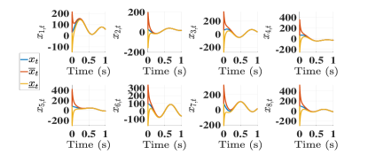
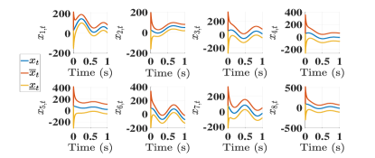
Figure 1: Estimation of $x_{t}\in\mathbb{R}^{8}$ in the absence and presence of $(d_{t},w_{t})$, above and below respectively, using observer (9).

3 Extension to LTV DT systems

In this section, our focus is on LTV systems. Since KKL results differ between CT and DT in this setting, let us restrict to DT systems, but similar results can indeed be derived in CT. First, it is important to recognize that finding a Jordan form for a time-varying matrix at each instant based on [2] is not realistic because the transformation’s closed form must be computed again at each time, thus the effectiveness of establishing an LTV change of coordinates $(R_{k})_{k\in\mathbb{N}}$ through the Jordan form as in [2] is very limited. However, our approach can easily deal with this matter through a systematic KKL-based LTV transformation. Second, compared to [4], while our change of coordinates is time-varying, the target system (12) is time-invariant in the dynamics part. This enables us to circumvent the necessity of requiring a common Lyapunov function for all time steps $k$ as in [4, Assumption 4], and eliminates the need for the restrictive assumption regarding the existence of a time-invariant change of coordinates for time-varying systems as in [4, Assumption 5]. Consider an LTV DT system

$$x_{k+1}=F_{k}x_{k}+U_{k}u_{k}+D_{k}d_{k},\quad y_{k}=H_{k}x_{k}+W_{k}w_{k},$$ (10)

where $(x_{k},y_{k},d_{k},w_{k})_{k\in\mathbb{N}}$ are defined in system (2) and $(F_{k},H_{k},U_{k},D_{k},W_{k})_{k\in\mathbb{N}}$ are known time-varying matrices.

Assumption 2.

For system (10), we assume that:

1. For all $k\in\mathbb{N}$, $F_{k}$ is invertible as $F_{k}^{-1}$;

2. There exist $c_{f}>0$ and $c_{h}>0$ such that for all $k\in\mathbb{N}$, we have $\|F_{k}^{-1}\|\leq c_{f}$ and $\|H_{k}\|\leq c_{h}$;

3. The pair $(F_{k},H_{k})$ is uniformly completely observable (UCO), i.e., there exist $m_{i}\in\mathbb{N}$, $i=1,2,\ldots,n_{y}$, and $c_{o}>0$ such that for all $k\geq\max m_{i}$, we have $\sum_{i=1}^{n_{y}}\sum_{j=k-m_{i}}^{k-1}\mathcal{O}_{i,j}^{\top}\mathcal{O}_{i,j}\geq c_{o}I$, where $\mathcal{O}_{i,j}=H_{i,j}F^{-1}_{j}\ldots F^{-1}_{k-2}F^{-1}_{k-1}$, with $H_{i,k}$ the $i^{\rm th}$ row of $H_{k}$;

4. There exist $\underline{x}_{0}$ and $\overline{x}_{0}$ such that $\underline{x}_{0}\leq x_{0}\leq\overline{x}_{0}$;

5. There exist known sequences $(\overline{d}_{k},\underline{d}_{k},\overline{w}_{k},\underline{w}_{k})_{k\in\mathbb{N}}$ such that $\underline{d}_{k}\leq d_{k}\leq\overline{d}_{k}$ and $\underline{w}_{k}\leq w_{k}\leq\overline{w}_{k}$ for all $k\in\mathbb{N}$.

Following the KKL paradigm [5], we strive for an LTV transformation $x_{k}\mapsto z_{k}:=T_{k}x_{k}$, where $(T_{k})_{k\in\mathbb{N}}$ is a sequence of matrices satisfying

$$T_{k+1}F_{k}=AT_{k}+BH_{k},\quad\forall k\in\mathbb{N},$$ (11)

where $A$ is Schur and non-negative, and $(A,B)$ is controllable, through which system (10) is put into

$$z_{k+1}=Az_{k}+By_{k}+T_{k+1}U_{k}u_{k}+T_{k+1}D_{k}d_{k}-BW_{k}w_{k}.$$ (12)

Note that because system (10) is LTV, $z_{k}\in\mathbb{R}^{n_{z}}$ and $T_{k}\in\mathbb{R}^{n_{z}\times n_{x}}$ for some $n_{z}\geq n_{x}$ to be defined later. We propose the following interval observer for system (12):

$$\left\{\begin{array}[]{@{}r@{\;}c@{\;}l@{}}\overline{z}_{k+1}&=&A\overline{z}_{k}+By_{k}+T_{k+1}U_{k}u_{k}+(T_{k+1}D_{k})^{\oplus}\overline{d}_{k}\\ &&{}-(T_{k+1}D_{k})^{\ominus}\underline{d}_{k}+(BW_{k})^{\ominus}\overline{w}_{k}-(BW_{k})^{\oplus}\underline{w}_{k}\\ \underline{z}_{k+1}&=&A\underline{z}_{k}+By_{k}+T_{k+1}U_{k}u_{k}+(T_{k+1}D_{k})^{\oplus}\underline{d}_{k}\\ &&{}-(T_{k+1}D_{k})^{\ominus}\overline{d}_{k}+(BW_{k})^{\ominus}\underline{w}_{k}-(BW_{k})^{\oplus}\overline{w}_{k},\end{array}\right.$$ (13a)

where the dynamics of $$T_{k}$$ can be updated, under Item (A2.1) of Assumption 2, as solution to (11) as

$$T_{k+1}=(AT_{k}+BH_{k})F_{k}^{-1},$$ (13b)

with any $$T_{0}\in\mathbb{R}^{n_{z}\times n_{x}}$$, in which

$$\overline{z}_{0}=T_{0}^{\oplus}\overline{x}_{0}-T_{0}^{\ominus}\underline{x}_{0},\quad\underline{z}_{0}=T_{0}^{\oplus}\underline{x}_{0}-T_{0}^{\ominus}\overline{x}_{0}.$$ (13c)

Similarly to the LTI case, we can show that (13a)-(13c) is an interval observer for system (12), so $$\underline{z}_{k}\leq z_{k}\leq\overline{z}_{k} k\in\mathbb{N} (T_{k}^{\dagger})_{k\in\mathbb{N}} (T_{k})_{k\in\mathbb{N}} T_{k}^{\dagger}T_{k}=I k\in\mathbb{N} k\in\mathbb{N} z x_{k} k\in\mathbb{N} z k^{\star}\in\mathbb{N} (T_{k})_{k\in\mathbb{N}_{\geq k^{\star}}} T_{k}^{\dagger}T_{k}=I k\in\mathbb{N}_{\geq k^{\star}} z k^{\star} k\in\mathbb{N}$$ for all . The Moore-Penrose inverse of is always defined but is not necessarily such that for all . Consequently, while it is feasible to design an interval observer for system (12) for all in the -coordinates, the technique used in Proposition 1 to recover the bounds of for every is not applicable here. Under Items (A2.2) and (A2.3) of Assumption 2 and with a right choice of the dynamics in the -coordinates as detailed in Proposition 3, there exists a finite linked to UCO beyond which the sequence becomes uniformly left-invertible and so for all [6]. This allows bringing back the bounds of the -coordinates observer (13a)-(13c) to design the bounds for system (10) after time . We then take for all ,

$$\overline{x}_{k} =(T_{k}^{\dagger})^{\oplus}\overline{z}_{k}-(T_{k}^{\dagger})^{\ominus}\underline{z}_{k},$$ (13d)

$$\underline{x}_{k} =(T_{k}^{\dagger})^{\oplus}\underline{z}_{k}-(T_{k}^{\dagger})^{\ominus}\overline{z}_{k},$$ (13e)

which recover the bounds of $x$ for all $k\in\mathbb{N}_{\geq k^{\star}}$. Note that in this time-varying setting, the $z$-coordinates can have a higher dimension than the $x$-coordinates, so we typically cannot write the observer in the $x$-coordinates as in observer (9). Such a design can still be done by adding fictitious states in the $x$-coordinates to equalize dimensions, but it has no clear interest compared to this. Our LTV design is recapped in the following proposition.

Proposition 3.

Suppose Assumption 2 holds and define $n_{z}=\sum_{i=1}^{n_{y}}m_{i}$ (with $m_{i}$ coming from Item (A2.3) of Assumption 2). Consider any $T_{0}\in\mathbb{R}^{n_{z}\times n_{x}}$ and for each $i\in\{1,2,\ldots,n_{y}\}$, a controllable pair $(\and_{i},\tilde{B}_{i})\in\mathbb{R}^{m_{i}\times m_{i}}\times\mathbb{R}^{m_{i}}$ with $\and_{i}$ Schur and non-negative. There exists $\gamma^{\star}\in(0,1]$ such that for any $0<\gamma<\gamma^{\star}$, there exist $k^{\star}\in\mathbb{N}$ and $(T_{k})_{k\in\mathbb{N}}$ where $T_{k}\in\mathbb{R}^{n_{z}\times n_{x}}$ is solution to (11) with

$$A =\gamma\and=\gamma\operatorname{diag}(\and_{1},\and_{2},\ldots,\and_{n_{y}})\in\mathbb{R}^{n_{z}\times n_{z}},$$ (14a)

$$B =\operatorname{diag}(\tilde{B}_{1},\tilde{B}_{2},\ldots,\tilde{B}_{n_{y}})\in\mathbb{R}^{n_{z}\times n_{y}},$$ (14b)

that is uniformly left-invertible after time $k^{\star}$, i.e., there exists $c_{T}>0$ such that $T_{k}^{\top}T_{k}\geq c_{T}I$ for all $k\in\mathbb{N}_{\geq k^{\star}}$. Then, observer (13) with the chosen $T_{0}$ is a finite-time interval observer for system (10), i.e., $\underline{x}_{k}\leq x_{k}\leq\overline{x}_{k}$ for all $k\in\mathbb{N}_{\geq k^{\star}}$.

Proof. From [6, Theorems 2 and 3] which are the nonlinear version of our case, under Assumption 2 and with the chosen $(A,B)$, the sequence $(T_{k})_{k\in\mathbb{N}}$ taking the dynamics (13b) and initialized as $T_{0}$ is solution to (11) and is uniformly left-invertible after a time, so $T_{k}^{\dagger}T_{k}=I$ for all $k$ after this time. The rest is proven similarly to Proposition 1, added with time variation of the matrices. $\blacksquare$

The following academic example illustrates our method.

Example 2.

Consider the system in [9, Example 2], with $F_{k}=\begin{pmatrix}1.2&1+0.5\cos(k)\\ 0&0.5+0.2\sin(k)\end{pmatrix}$ and $H_{k}=\begin{pmatrix}1&0\end{pmatrix}$. It is not obvious to find classical transformations for this time-varying system. From [9], the pair $(F_{k},H_{k})$ is UCO with $m=2$, and Items (A2.1) and (A2.2) of Assumption 2 are satisfied. Pick $\tilde{A}=\begin{pmatrix}0.1&0\\ 0&0.2\end{pmatrix}$ and $\tilde{B}=\begin{pmatrix}1\\ 1\end{pmatrix}$, so $A=\gamma\tilde{A}$ is both Schur and non-negative, and then with $\gamma=1$, $(T_{k})_{k\in\mathbb{N}}$ is uniformly left-invertible after $k^{\star}=2$. Consider disturbance $d_{k}=0.1(\sin(2k),-\sin(2k))$, noise $w_{k}=0.02\cos(20k)$ with unit gains, and assume known bounds for these. Observer (13) is then designed for this system. Due to space constraints, we show in Figure 2 the results for only the second state, which is not measured. We see that the framer property is only guaranteed after $k^{\star}$ when we have gathered enough observability.

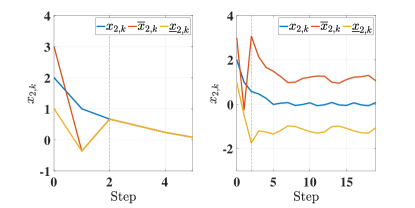
Figure 2: Finite-time estimation of $x_{2,k}$ in the absence and presence of disturbances/noise using observer (13).

4 Conclusion

We introduce systematic interval observer designs for linear systems. Diverging from current methods, our approach boasts straightforward implementation and requires standard assumptions, with only a constant, easy-to-compute matrix $T$ to guarantee both positivity and stability for LTI interval observer design for an LTI system. The interval observer design procedure for LTI systems can now be as straightforward as Algorithm 1. Our method also extends to LTV systems, offering a unified method for interval observer design for linear systems.

Note that even if the matrix $F$ in system (1) contains complex components, our method should remain applicable as it is based on solving a Sylvester equation. However, the methods presented in [1, 2] may not be suitable as they rely on Jordan forms of real matrices. Also, due to the high freedom of $(A,B)$, these can be tailored for bound optimization purposes. Future work includes how to effectively optimize the bounds in Algorithm 1 through the choice of $(A,B)$ to improve performance.

The authors thank Pauline Bernard for her constructive remarks that improved this paper.

References

• [1] F. Mazenc and O. Bernard, “Interval observers for linear time-invariant systems with disturbances,” Automatica, vol. 47, no. 1, pp. 140–147, April 2011.
• [2] F. Mazenc, T. N. Dinh, and S.-I. Niculescu, “Interval observers for discrete-time systems,” International Journal of Robust and Nonlinear Control, vol. 24, no. 17, pp. 2867–2890, 2014.
• [3] T. Ras̈si, D. Efimov, and A. Zolghadri, “Interval state estimation for a class of nonlinear systems,” IEEE Transactions on Automatic Control, vol. 57, no. 1, pp. 260–265, 2012.
• [4] D. Efimov, W. Perruquetti, T. Raïssi, and A. Zolghadri, “Interval observers for time-varying discrete-time systems,” IEEE Transactions on Automatic Control, vol. 58, no. 12, pp. 3218–3224, 2013.
• [5] D. G. Luenberger, “Observing the state of a linear system,” IEEE Transactions on Military Electronics, vol. 8, no. 2, pp. 74–80, 1964.
• [6] G. Q. B. Tran and P. Bernard, “Arbitrarily fast robust KKL observer for nonlinear time-varying discrete systems,” IEEE Transactions on Automatic Control, vol. 69, no. 3, pp. 1520–1535, 2024.
• [7] Z. Zhang and J. Shen, “A survey on interval observer design using positive system approach,” Franklin Open, vol. 4, p. 100031, 2023.
• [8] T. N. Dinh, F. Mazenc, and S.-I. Niculescu, “Interval observer composed of observers for nonlinear systems,” in 13th European Control Conference, 2014, pp. 660–665.
• [9] Q. Zhang, “On stability of the Kalman filter for discrete time output error systems,” Systems and Control Letters, vol. 107, pp. 84–91, Jul. 2017.