Low-rank quantics tensor train representations of Feynman diagrams for
multiorbital electron-phonon models

Abstract

Feynman diagrams are an essential tool for simulating strongly correlated electron systems. However, stochastic quantum Monte Carlo (QMC) sampling suffers from the sign problem, e.g., when solving a multiorbital quantum impurity model. Recently, two approaches have been proposed for efficient numerical treatment of Feynman diagrams: Tensor Cross Interpolation (TCI) for replacing the stochastic sampling and the Quantics Tensor Train (QTT) representation for compressing space-time dependence. Combining these approaches, we find low-rank structures in weak-coupling Feynman diagrams for a multiorbital electron-phonon model and demonstrate their efficient numerical integrations with exponential resolution in time and exponential convergence of error with respect to computational cost.

In diverse fields ranging from condensed matter physics to high-energy physics, calculations based on Feynman diagrams in quantum field theory have become indispensable [1]. Numerical perturbative calculations often involve numerical integrations and summations over virtual times and internal degrees of freedom of these diagrams. However, when dealing with multiorbital models or higher-order diagrams, straightforward numerical integration faces the notorious “curse of dimensionality,” leading to exorbitant computational times. Consequently, methods to circumvent this curse in quantum field theory calculations are in high demand.

Various approaches have been explored to address this challenge. For instance, quantum Monte Carlo (QMC) methods [2, 3, 4, 5], grounded in importance sampling in multidimensional spaces, are widely employed. Yet, in complex systems, these methods suffer from the negative sign problem, causing computational times to explode exponentially [6, 7, 8, 9, 10]. This occasionally hinders accessing parameter regimes with physically interesting phenomena.

A recent breakthrough has been the introduction of Tensor Cross Interpolation (TCI), which employs tensor networks to learn a function and perform its integration in multidimensional spaces [11]. The TCI approach is based on low-rank structures hidden in a function. This method has demonstrated its prowess by calculating physical quantities with unprecedented precision in various models, outperforming the Monte Carlo methods in some cases, e.g., in solving single-orbital quantum impurity models [11, 12]. They observed that the integration error in TCI converges more rapidly than in QMC sampling, following a rate of $O(1/n_{\mathrm{s}}^{a})$, with $a>1/2$, where $n_{\mathrm{s}}$ denotes the number of integrand evaluations. Yet, determining the factors influencing this convergence rate remains unresolved. Furthermore, extending the TCI method to multiorbital systems and electron-phonon coupling remains to be developed, which is essential for its practical application in materials calculations.

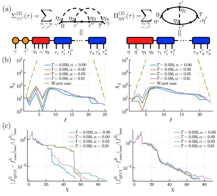
Figure 1: (a) Second-order skeleton diagrams for the electron self-energy $\Sigma^{(2)}$ and phonon self-energy $\Pi^{(2)}$, as well as tensor train (TT) representations of their integrands. (b) Bond dimensions $\chi_{\ell}$ for TCI tolerance $\epsilon=10^{-3}$ for typical parameters set above/below the superconducting temperature $T_{\mathrm{c}}\simeq 0.2$ and with/without an external field, whose strength is denoted by $\alpha$. We employed a virtual $2^{{\mbox{$\mathcal{R}$}}}\times 2^{{\mbox{$\mathcal{R}$}}}\times 2^{{\mbox{$\mathcal{R}$}}}$ grid for $\tau$, $\tau^{\prime}$ and $\tau^{\prime\prime}$ (${{\mbox{$\mathcal{R}$}}}=20$, $2^{{\mbox{$\mathcal{R}$}}}\simeq 10^{6}$). (c) Interpolation error estimate as a function of bond dimension $\chi$. The error is normalized by an estimate of the absolute maximum of the function (integrand).

In a complementary vein, a novel discretization technique for space-time based on the quantics tensor train (QTT) has been proposed for solving Navier-Stokes equations for turbulent flows [13, 14], the Vlasov-Poisson equations for collisionless plasmas [15], and solving diagrammatic equations in quantum field theories [16]. The QTT method leverages the low-entanglement structures between exponentially different length scales, allowing for an exponential enhancement in spatiotemporal resolution relative to data volume and computational effort. In Ref. [16], the separation in length scales has been showcased in various multidimensional spacetime datasets of correlation functions in quantum field theories, including momentum dependence of one-particle Green’s function, three-frequency dependence of a vertex function at the two-particle level and so on.

Furthermore, the amalgamation of TCI and QTT has given birth to the quantics tensor cross interpolation (QTCI) technologies [17]. They illustrated its potential with an application from condensed matter physics: the computation of Brillouin zone integrals [17]. Applications of QTCI to more complex cases, e.g., integration over both continuous and discrete variables, are promising and remain to be explored.

The primary objective of this study is to address the following questions: (i) Do low-rank tensor train (TT) structures exist within self-energy Feynman diagrams for multiorbital systems? (ii) Is the TCI robust for interpolating complex integrands with continuous and discrete degrees of freedom? (iii) Can TCI accommodate phonon contributions, which, despite their physical relevance, occasionally worsens the sign problem in QMC simulations? (iv) Does employing quantics facilitate achieving an enhanced convergence rate, specifically exponential convergence? To investigate these questions, as a first step, we analyze weak-coupling self-energy Feynman diagrams in the imaginary-time formalism for a prototype multiorbital electron-phonon model, originally proposed for exploring superconducting states in fullerides [18, 19, 20, 21, 22].

Figure 1 summarizes our main results obtained with and without an external field. Figure 1(a) illustrates the TT structures proposed in this study for the electron and phonon self-energies, where imaginary-time variables are discretized by the quantics representation. Discrete internal and external variables, such as spin-orbital indices $\gamma$ and vibrational modes of phonon $\eta$ are encoded in the same TT as well. As shown in Fig. 1(b), the bond dimensions of the TT representations obtained by TCI are much smaller than the worst case of incompressible functions, establishing the existence of low-rank structures. As demonstrated in Fig. 1(c), the interpolation error estimate in the TCI vanishes exponentially regardless of the superconducting transition and the presence of the external field, indicating the advantage of the QTT representation.

The Hamiltonian of the model reads

$$\mathscr{H} =\sum_{ij}\sum_{\gamma\gamma^{\prime}\sigma}\left(t^{\gamma\gamma^{\prime}}_{ij}-\mu\delta_{ij}\delta_{\gamma\gamma^{\prime}}\right)c^{\dagger}_{i\gamma\sigma}c_{j\gamma^{\prime}\sigma}+\sum_{i\eta}\omega_{\eta}a^{\dagger}_{i\eta}a_{i\eta}$$

$$\quad+\sum_{i\eta}I_{\eta}:T_{i\eta}T_{i\eta}:+\sum_{i\eta}g_{\eta}\phi_{i\eta}T_{i\eta},$$ (1)

where $\gamma=x,y,z$ represent the $t_{1u}$ electronic orbitals, $\eta=0,1,3,4,6,8$ correspond to the six vibrational modes of a fullerene molecule with energies $\omega_{\eta}$, and $c^{\dagger}$ and $c$ are the creation and annihilation operators for electrons, respectively, while $a^{\dagger}$ and $a$ are the creation and annihilation operators for phonons. The $\lambda^{\eta}$ are Gell-Mann matrices, $T_{i\eta}=\sum_{\gamma\gamma^{\prime}\sigma}c^{\dagger}_{i\gamma\sigma}\lambda^{\eta}_{\gamma\gamma^{\prime}}c_{i\gamma^{\prime}\sigma}$, $\phi_{i\eta}=a_{i\eta}+a^{\dagger}_{i\eta}$, $I_{\eta}=(3/4)U-J$ ($\eta=0$), $=J/2$ (otherwise) . The first term represents inter-site hopping $t_{ij}$ and the chemical potential $\mu$. The non-interacting part of the Hamiltonian is given by the semicircular non-interacting density of states of width 1. The second term gives the single-particle phonon energies. The third term represents instantaneous local Columb interactions, where the ($:$) symbol represents the normal ordering. The fourth term denotes the electron-phonon couplings. For more details on the model, we refer the reader to Ref. 22.

We take $\omega_{\eta}=\omega_{0}=0.15$ and $g_{\eta}=g_{0}=\sqrt{3\lambda_{0}\omega_{0}/4}$ with $\lambda_{0}=0.15$. We set $U=J=\mu=0$ and consider only the electron-phonon interaction to investigate low-rank structures hidden in Feynmann diagrams functions. Numerical treatment of the instantaneous part will be more straightforward.

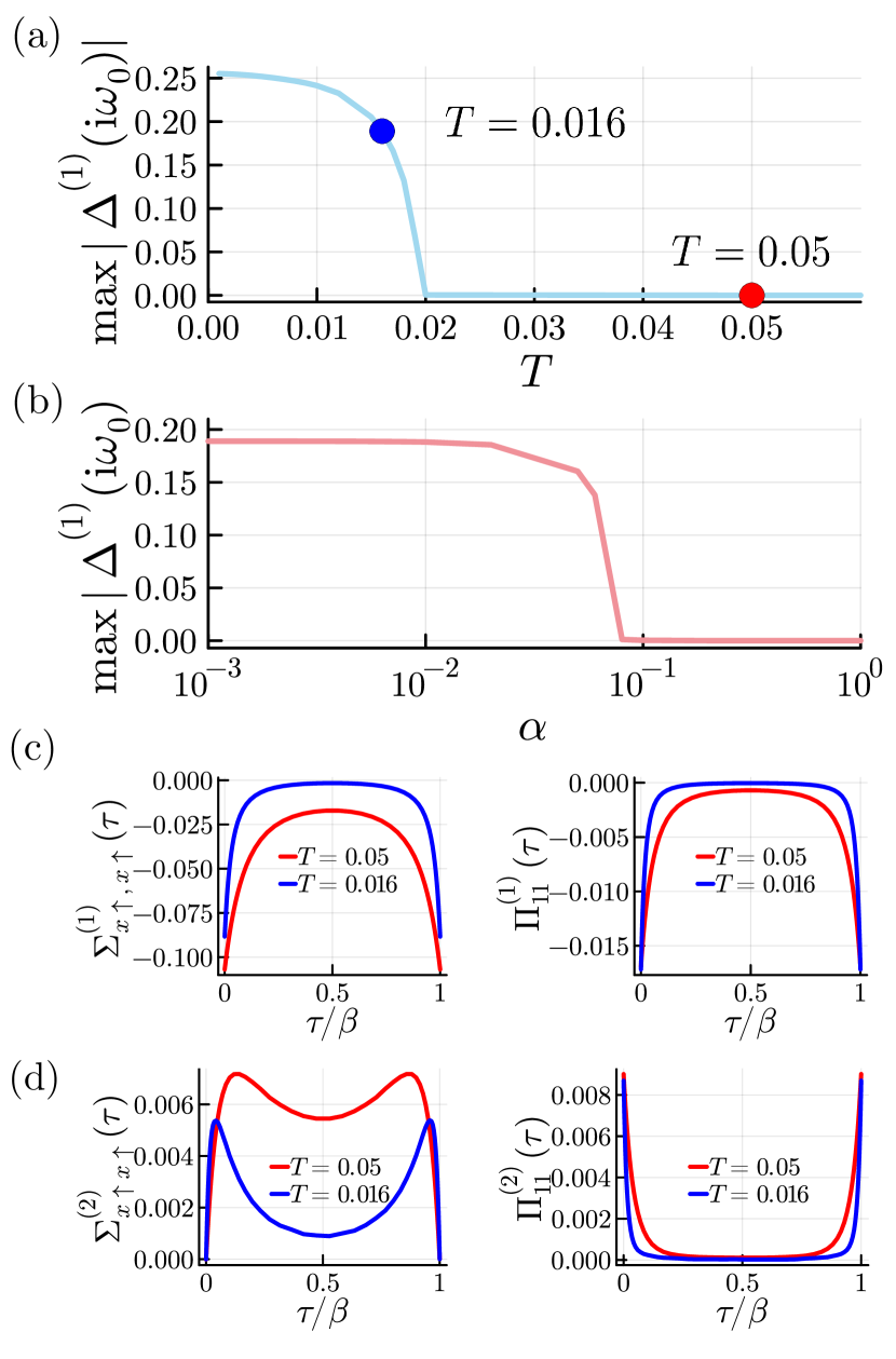
Figure 2: (a) $T$ dependence of the absolute maximum of the gap function with no external field ($\alpha=0$). (b) $\alpha$ dependence of the absolute maximum of the gap function at $T=0.016$. (c) $\Sigma^{(1)}$ and $\Pi^{(1)}$ computed at $T=0.05,~{}0.016$ with $\alpha=0$. (d) $\Sigma^{(2)}$ and $\Pi^{(2)}$ computed at $T=0.05,~{}0.016$ with $\alpha=0$.

We solve the model within the dynamical-mean field theory by assuming local self-energies. The local Green’s function in the Nambu basis reads

$$\check{G}_{\gamma\sigma,\gamma^{\prime}\sigma^{\prime}}(\tau) =-\expectationvalue{\mathcal{T}\Psi(\tau)\Psi^{\dagger}(0)}=\left(\begin{smallmatrix}G_{\gamma\sigma,\gamma^{\prime}\sigma^{\prime}}(\tau)&F_{\gamma\sigma,\gamma^{\prime}\sigma^{\prime}}(\tau)\\ \bar{F}_{\gamma\sigma,\gamma^{\prime}\sigma^{\prime}}(\tau)&\bar{G}_{\gamma\sigma,\gamma^{\prime}\sigma^{\prime}}(\tau)\end{smallmatrix}\right),$$

$$D_{\eta\eta^{\prime}}(\tau) =-\expectationvalue{\mathcal{T}\phi_{\eta}(\tau)\phi_{\eta^{\prime}}(0)},$$

where $\Psi(\tau)=(c_{x\uparrow}(\tau),c_{x\downarrow}(\tau),\cdots,c_{z\downarrow}(\tau),c^{\dagger}_{x\uparrow}(\tau),\cdots,c^{\dagger}_{z\downarrow}(\tau))^{\!\top}$, $c_{\gamma\sigma}(\tau)$/$c_{\gamma\sigma}^{\dagger}(\tau)$ represents an annihilation/creation operator for orbital $\gamma$ and spin $\sigma$ in the Heisenberg picture, $\mathcal{T}$ indicates time odering.

Note that matrices with a checkmark $\check{}$, such as $\check{A}$, are defined in the Nambu space and have a shape of $12\times 12$.

A weak-coupling expansion yields the following connected skeleton diagrams for the electron and phonon self-energies [Fig. 1(a)]:

$$\check{\Sigma}^{(1)}(\tau)=-\sum_{\eta_{1}\eta_{2}}g_{0}^{2}D_{\eta_{1}\eta_{2}}(\tau)\check{\lambda}^{\eta_{1}}\check{G}(\tau)\check{\lambda}^{\eta_{2}},$$ (2)

$$\check{\Sigma}^{(2)}(\tau)=\int_{[0,\beta]^{2}}d\tau^{\prime}d\tau^{\prime\prime}\sum_{\eta_{1}\eta_{2}\eta_{3}\eta_{4}}g_{0}^{4}D_{\eta_{1}\eta_{3}}(-\tau^{\prime\prime})D_{\eta_{2}\eta_{4}}(\tau^{\prime}-\tau)$$

$$~{}~{}~{}\times\check{\lambda}^{\eta_{4}}\check{G}(\tau-\tau^{\prime\prime})\check{\lambda}^{\eta_{3}}\check{G}(\tau^{\prime\prime}-\tau^{\prime})\check{\lambda}^{\eta_{2}}\check{G}(\tau^{\prime})\check{\lambda}^{\eta_{1}},$$ (3)

$$\Pi^{(1)}_{\eta\eta^{\prime}}(\tau)=\dfrac{1}{2}g_{0}^{2}\Tr\left[\check{G}(-\tau)\check{\lambda}^{\eta^{\prime}}\check{G}(\tau)\check{\lambda}^{\eta}\right],$$ (4)

$$\Pi^{(2)}_{\eta\eta^{\prime}}(\tau)=-\dfrac{1}{2}\int_{[0,\beta]^{2}}d\tau^{\prime}d\tau^{\prime\prime}\sum_{\eta_{2}\eta_{4}}g_{0}^{4}D_{\eta_{2}\eta_{4}}(\tau^{\prime}-\tau^{\prime\prime})\times$$

$$~{}{\rm Tr}\left[\check{G}(-\tau^{\prime\prime})\check{\lambda}^{\eta_{4}}\check{G}(\tau^{\prime\prime}-\tau)\check{\lambda}^{\eta}\check{G}(\tau-\tau^{\prime})\check{\lambda}^{\eta_{2}}\check{G}(\tau^{\prime})\check{\lambda}^{\eta^{\prime}}\right].,$$ (5)

where $\beta=1/T$ denotes inverse temperature. The Gell-Mann matrix in the Nambu space reads $\check{\lambda}^{\eta}=\mathcal{N}(\lambda^{\eta}\otimes\mathbf{1}_{2\times 2})$, where $\mathbf{1}_{2\times 2}$ is the unit matrix in spin space ($2\times 2$) and $\check{M}=\mathcal{N}(M)\equiv\left(\begin{smallmatrix}M&0\\ 0&-M^{\!\top}\end{smallmatrix}\right)$. The electron’s self-energy, denoted by $\check{\Sigma}$, is defined as a $12\times 12$ matrix in the form of

$$\check{\Sigma}(\tau)=\begin{pmatrix}\Sigma(\tau)&\Delta(\tau)\\ \Delta^{\dagger}(\tau)&-\Sigma^{\!\top}(-\tau)\end{pmatrix}\equiv\begin{pmatrix}\left(\check{\Sigma}\right)_{11}&\left(\check{\Sigma}\right)_{12}\\ \left(\check{\Sigma}\right)_{21}&\left(\check{\Sigma}\right)_{22}\\ \end{pmatrix},$$ (6)

where $\Delta(\tau)$, referred to as the gap function, is a $6\times 6$ matrix. The phonon Green’s function $D$ and the self-energy $\Pi$ are $6\times 6$ matrix.

The self-consistent equations read

$$\!\!\!\check{G}({\rm i}\omega_{n})\! =\!\!\int\!d\varepsilon\rho(\varepsilon)\!\left[{\rm i}\omega_{n}\mathbf{1}_{12\times 12}\!+\!(\mu-\varepsilon)\check{\mathbf{1}}\!-\!\check{\Sigma}({\rm i}\omega_{n})\!-\!\alpha\mathscr{H}_{\mathrm{ex}}\right]^{-1},$$

$$D({\rm i}\nu_{m}) =D^{(0)}({\rm i}\nu_{m})[\mathbf{1}_{6\times 6}-D^{(0)}({\rm i}\nu_{m})\Pi({\rm i}\nu_{m})]^{-1}$$

where $\omega_{n}$ and $\nu_{m}$ are Matsubara frequencies for fermions and bosons, $\mathbf{1}_{N\times N}$ is the $N\times N$ unit matrix, $\check{\mathbf{1}}\equiv\mathcal{N}(\mathbf{1}_{6\times 6})$ and $\rho(\varepsilon)=(8/\pi)\sqrt{(1/2)^{2}-\varepsilon^{2}}$ , $D_{\eta\eta^{\prime}}^{(0)}({\rm i}\nu_{m})=2\delta_{\eta\eta^{\prime}}\omega_{0}/(({\rm i}\nu_{m})^{2}-\omega_{0}^{2})$ is the non-interacting phonon Green’s function.

We can apply an external field with $\alpha\neq 0$. We apply the external field to lower the symmetry to examine cases where the symmetry is reduced. Here, we chose $\mathscr{H}_{\mathrm{ex}}=\mathcal{N}(l_{z}\otimes\mathbf{1}_{2\times 2})$ as a test field. Here, $l_{z}=\left(\begin{smallmatrix}0&-{\rm i}&0\\ {\rm i}&0&0\\ 0&0&0\end{smallmatrix}\right)$ represents the orbital magnetic field. $\alpha$ denotes the magnitude of the external field.

We perform self-consistent calculations with $\Sigma^{(1)}$ and $\Pi^{(1)}$ using the sparse modeling methods based on the intermediate representation (IR) [23, 24, 25] to describe a superconducting state. The resultant Green’s functions are stored in IR and can be evaluated at any $\tau$. This first-order solution is used for the evaluation of the more complex second-order diagrams involving imaginary time integrals.

Quantics tensor train We start with introducing the quantics representation of a univariate function, denoted by $f(x):x\in[0,1)\rightarrow\mathbb{C}$. The function can be “tensorized” by binary notation [26, 27, 16]. In practice, we construct an equidistant grid on the interval $[0,1)$: $x=(0.\sigma_{1}\sigma_{2}\dots\sigma_{{{\mbox{$\mathcal{R}$}}}})_{2}=\sum_{r=1}^{{{\mbox{$\mathcal{R}$}}}}\sigma_{r}2^{-r}$, where $\sigma_{r}\in\{0,1\}$ corresponds to the scale $2^{-r}$. We then decompose the $\mathcal{R}$-way tensor, $F_{\sigma_{1},\dots,\sigma_{{{\mbox{$\mathcal{R}$}}}}}\equiv f((0.\sigma_{1}\cdots\sigma_{{\mbox{$\mathcal{R}$}}})_{2})$, as

$$F_{\sigma_{1},\sigma_{2},\cdots,\sigma_{{{{\mbox{$\mathcal{R}$}}}}}}\approx\sum_{\alpha_{1}}^{\chi_{1}}\cdots\sum_{\alpha_{{{{\mbox{$\mathcal{R}$}}}}-1}}^{\chi_{{{{\mbox{$\mathcal{R}$}}}}-1}}F^{(1)}_{\sigma_{1}\alpha_{1}\alpha_{2}}\cdots F^{({{\mbox{$\mathcal{R}$}}})}_{\sigma_{{{{\mbox{$\mathcal{R}$}}}}}\alpha_{{{{\mbox{$\mathcal{R}$}}}}-1}},$$ (7)

$$\hskip 20.00003pt\raisebox{-0.5pt}{\includegraphics[width=173.44534pt]{schematic_QTT.pdf}}~{},$$ (8)

where $F_{\sigma_{1},\dots,\sigma_{{{\mbox{$\mathcal{R}$}}}}}$ has a total of $2^{{\mbox{$\mathcal{R}$}}}$ elements, and $F^{(\ell)}$ is a three-way tensor of size $2\times\chi_{\ell-1}\times\chi_{\ell}$. The sizes of the auxiliary indices (virtual bonds) $\alpha_{\ell}$, $\chi_{\ell}$, are referred to as bond dimensions. The bond dimension of the TT is defined as $\chi\equiv\mathrm{max}_{\ell}~{}\chi_{\ell}$. The integral of $f(x)$ can be evaluated accurately by Riemann summation as

$$\raisebox{-0.5pt}{ \includegraphics[width=433.62pt]{TT_int.pdf} }~{},$$

where denotes the vector $(1/2,1/2)$. In the above equation, the first $\simeq$ denotes the approximation by the Riemann sum, where the discretization error can be negligibly and exponentially small as $O(2^{-2{{\mbox{$\mathcal{R}$}}}})$. The second $\simeq$ corresponds to the TT approximation. The computational time of the contraction scales linearly with $\mathcal{R}$ as $O(\chi^{2}{{\mbox{$\mathcal{R}$}}})$.

The exact representation of an incompressible function, for example, a random function, requires $\chi_{\ell}$ to grow toward the center of the TT exponentially, offering no memory advantage over $F_{x_{1},\dots,x_{{{\mbox{$\mathcal{R}$}}}}}$. In the presence of a low-rank structure in $F$, i.e., the separation between different length scales [16], the bond dimension can be significantly reduced; as a result, the total number of elements in the TT grows only linearly with $\mathcal{R}$ as $\mathcal{O}(\chi^{2}{{\mbox{$\mathcal{R}$}}})$. The imaginary-time dependence of propagators self-energies is expected to have such low-rank structures [16, 28].

TT representations for integrands The integrands of self-energies (3) and (5) depend on multiple discrete and continuous variables. For example, the integrand of the electron self-energy (3) depends on discrete variables $\gamma,\gamma^{\prime},\eta_{1},\eta_{2},\eta_{3},\eta_{4}$, and continuous variables $\tau,\tau^{\prime},\tau^{\prime\prime}$. We apply the binary coding to the continuous variables as $\tau/\beta=(0.\tau_{1}\cdots\tau_{{{\mbox{$\mathcal{R}$}}}})_{2}$, $\tau^{\prime}/\beta=(0.\tau^{\prime}_{1}\cdots\tau^{\prime}_{{{\mbox{$\mathcal{R}$}}}})_{2}$, $\tau^{\prime\prime}/\beta=(0.\tau^{\prime\prime}_{1}\cdots\tau^{\prime\prime}_{{{\mbox{$\mathcal{R}$}}}})_{2}$. Figure 1(a) illustrates the TTs for the integrands. The lengths of the TTs are ${{\mbox{$\mathcal{L}$}}}=3{{\mbox{$\mathcal{R}$}}}+6$ and ${{\mbox{$\mathcal{L}$}}}=3{{\mbox{$\mathcal{R}$}}}+4$, respectively. We assign $\tau_{r}$, $\tau^{\prime}_{r}$, $\tau^{\prime\prime}_{r}$, at the same length scale to the same tensor due to the strong entanglement between these degrees of freedom [16, 28]. The indices for the discrete variables are grouped on the left side of the TTs.

Tensor cross interpolation (TCI) We construct a TT for the integrand by TCI, which is an adaptive learning algorithm that constructs a low-rank TT from a small subset of adaptively chosen elements of a tensor $T$ (interpolation points). Specifically, it optimizes $\chi_{\ell}$ so that a global error estimate satisfies $\|T-\tilde{T}\|_{\mathrm{max}}/\|T\|_{\mathrm{max}}<\epsilon$, where $\epsilon$ is a tolerance, $\tilde{T}$ is a TT and $\|\cdots\|_{\mathrm{max}}$ denotes the maximum norm. Generally, the number of interpolation points required for constructing a TT with length $\mathcal{L}$ and bond dimension $\chi$ scales linearly with $\mathcal{R}$ as $O(\chi^{2}\mathcal{L})$, leading to an exponential speed-up over the conventional tensor decomposition based on singular value decomposition. For details, please refer to Ref. [29].

For constructing a TT for the integrand, we evaluate the RHS of Eq. (3) and Eq. (5) for indices chosen by TCI. This can be performed straightforwardly if the $\tau$ dependence of the Green’s functions is expanded by IR. The function evaluations consume the majority of the computational time of the TT construction. We explored the configuration space by combining 2-site (local) updates [29] and global moves [30]. We found that the use of the global moves is necessary for a stable convergence of the TCI: The 2-site updates suffer from an ergodicity problem [29].

Integration over internal variables Once the TT representation is constructed, summation and integration over the internal variables can be performed efficiently, as explained above. For instance, the TT representation of the electron self-energy (3) can be constructed as 

$$\raisebox{-0.5pt}{ \includegraphics[width=368.57964pt]{TT.pdf}},$$

where the tensor with no leg (red) can be absorbed into either its left (for $\gamma^{\prime}$) or right (for $\tau_{1}$) tensor. The resultant TT can be readily evaluated at any point $(\gamma,\gamma^{\prime},\tau)$ with exponentially high resolution for $\tau$.

We first discuss the $\alpha$-$T$ phase diagram. Figure 2(a) plots the $T$ dependence of the order parameter of the superconducting transition. The system exhibits a second-order phase transition into a superconducting phase around $T=0.02$, being consistent with the results in the previous study [22]. Figure 2(b) shows the $\alpha$ dependence of the order parameter at $T=0.016$. The order parameter vanishes around $\alpha=0.08$, signaling a transition to the normal phase.

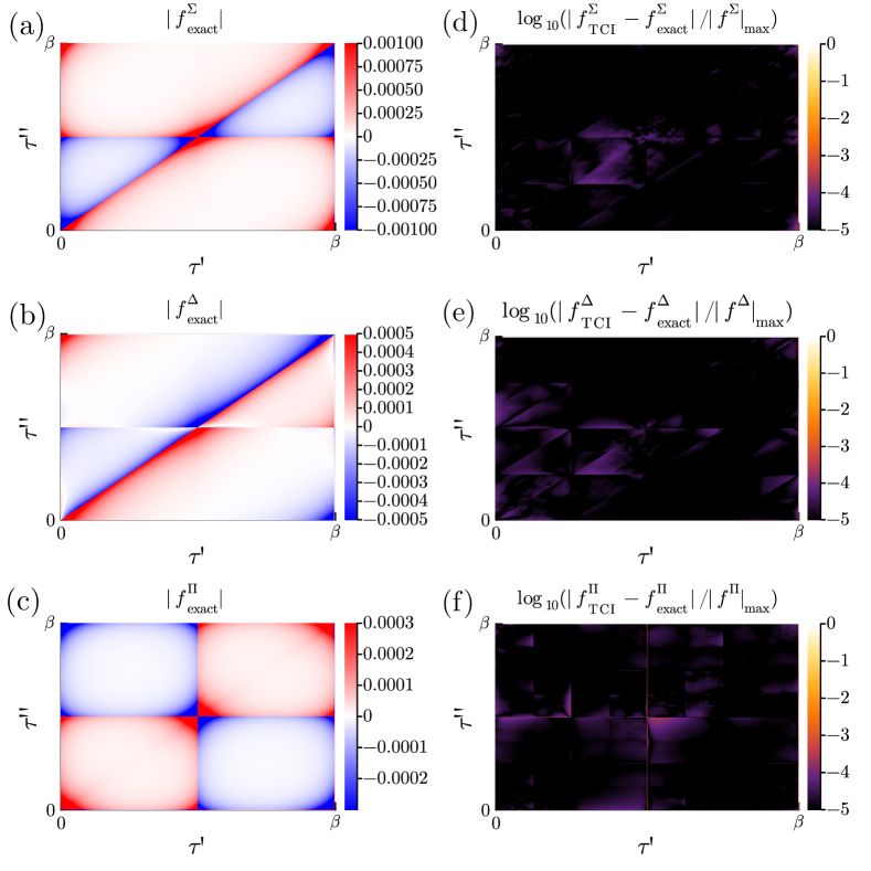
Figure 3: Integrands of (a) $\Sigma^{(2)}_{x\uparrow,x\uparrow}$, (b) $\Delta_{x\uparrow,x\downarrow}^{(2)}$, and (c) $\Pi^{(2)}_{11}$ at $\tau=\beta/2$ and $T=0.016$. Panels (d)–(f) show interpolation errors with $\epsilon=10^{-3}$ for the integrands in (a)–(c), respectively.

Figure 2(c) shows typical self-energies $\Sigma^{(1)}$ and $\Pi^{(1)}$ computed at $T=0.05$ ($>T_{\mathrm{c}}$) and $T=0.016$ ($<T_{\mathrm{c}}$) for $\alpha=0$. Let us discuss the structures of the self-energy matrices in the flavor space. At $\alpha=0$ and $T>T_{\mathrm{c}}$, the normal part of the electron self-energy $\Sigma^{(1)}(\tau)$ and the bosonic self-energy $\Pi^{(1)}(\tau)$ are diagonal, while the anomalous part of the electron self-energy $\Delta^{(1)}(\tau)=0$. At $\alpha=0$ and for $T<T_{\mathrm{c}}$, the spontaneous symmetry breaking gives rise to nonzero superdiagonal and subdiagonal elements in $\Delta^{(1)}(\tau)$. Introducing $\alpha>0$ further reduces the symmetry. We observed that nonzero components appear in $(\gamma\sigma,\gamma^{\prime}\sigma^{\prime})=(x\!\!\uparrow,y\!\!\uparrow),(x\!\!\downarrow,y\!\!\downarrow)$ for $\Sigma$, $(\gamma\sigma,\gamma^{\prime}\sigma^{\prime})=(x\!\!\uparrow,y\!\!\downarrow),(x\!\!\downarrow,y\!\!\uparrow)$ for $\Delta$, and $(\eta,\eta^{\prime})=(1,3),(4,6),(0,8)$ for $\Pi$, respectively. This refers to the upper triangular part, and nonzero components also appear symmetrically in the lower triangular part. The appearance of these nonzero components is consistent with what is expected from the symmetry of the external field. The second-order self-energy matrices have precisely the same structures of nonzero elements as those of the first-order self-energies.

The left panels of Fig. 3 show typical components of the integrands for $\Sigma^{(2)}$, $\Delta^{(2)}$, and $\Pi^{(2)}$ computed at $\alpha=0$ and $T=0.016$. These integrands have several lines of discontinuities, originating from the discontinuity of the one-particle propagators at $\tau=n\beta$ ($n\in\mathbb{Z}$).

We now construct TCIs of these functions for typical parameter sets of $T$ and $\alpha$. The tolerance is set to $\epsilon=10^{-3}$. The TCI construction takes a few minutes with one Apple M2 CPU core for $\chi\simeq 100$.

The results are shown in Fig. 1(b). We numerically confirmed that the constructed $\tau$-dependent $12\times 12$ matrix $\check{\Sigma}$ satisfies the expected relation between the blocks: $\left(\check{\Sigma}\right)_{11}(\tau)=-\left(\check{\Sigma}\right)_{22}^{\!\top}(-\tau)$ and $\left(\check{\Sigma}\right)_{12}(\tau)=\left(\check{\Sigma}\right)_{21}^{\dagger}(\tau)$ . This indicates the stability of the TCI.

Figure 1(b) shows the bond dimensions $\chi_{\ell}$ computed for typical parameter sets. The bond dimensions are significantly smaller than the worst (incompressible) case and strongly depend on $\ell$. For the electron self-energy, $\chi_{\ell}$ takes large values at $\ell=4$ (between $\eta_{2}$ and $\eta_{3}$) and at $\ell\simeq 8$. The bond $\ell=8$ connects the time scales of $\tau/\beta=2^{-2}$ ($r=2$) and $2^{-3}$ ($r=3$). For shorter time scales, $\chi_{\ell}$ monotonically decreases, allowing us to increase the time resolution exponentially. We observed a similar trend for the phonon self-energy: $\chi_{\ell}$ takes large values around $\ell=6$, corresponding to between $r=2$ and $r=3$.

We move on to a more detailed discussion on the compactness of the quantics representation. Figure 1(c) shows the $\chi$ dependence of an estimate of the interpolation error. The interpolation error for all the parameter sets eventually decreases exponentially with $\chi$. Let us first focus on the cases with no external field ($\alpha=0$) in more depth. Comparing the results for $T=0.02~{}(>T_{\mathrm{c}})$ and $T=0.016~{}(<T_{\mathrm{c}})$, one can see that the symmetry breaking roughly doubles $\chi$ required to reach $\epsilon=10^{-2}$ from $\simeq 35$ to $\simeq 55$. This can be attributed to the emergence of the nonzero components in $\check{\Sigma}$.

At $T=0.016$, increasing $\alpha=0$ to $\alpha=0.05$ in the superconducting phase does not change the behavior of the interpolation error above $\epsilon=10^{-2}$ qualitatively but leads to the emergence of a more slowly decaying tail below $\epsilon=10^{-2}$. This tail may originate from the requirement of interpolating the small off-diagonal components in $\check{\Sigma}$ induced by the external field. Further increasing $\alpha$ beyond the transition point, $\chi$ becomes substantially smaller with the disappearance of the spontaneous symmetry breaking.

The right panels of Fig. 3 show the interpolation error in the reconstructed self-energy for a typical parameter set, $T=0.016$ and $\alpha=0$. One can clearly see that the interpolation does not suffer from the discontinuity. The interpolation error has block-like structures, which are consistent with the binary coding.

We now demonstrate the integration of internal variables in the TT format. Once we obtain the integrated TT, we can readily evaluate it at any $\tau$ and flavor pair. Figure 2(d) shows the self-energy evaluated on a dense grid for the typical components. Note that $\Sigma^{(2)}$ and $\Pi^{(2)}$ are much smaller than $\Sigma^{(1)}$ and $\Pi^{(1)}$ in amplitude, justifying the validity of the one-shot calculation of $\Sigma^{(2)}$ and $\Pi^{(2)}$. The $\tau$ dependence of $\Sigma^{(2)}$ and $\Pi^{(2)}$ does not exhibit any signature of the discretization due to the exponential resolution. We further tested the correctness of the evaluated self-energies by projecting them onto the IR basis: We confirmed that the expansion coefficient decays as fast as expected (not shown).

In this letter, we studied the low-rank structures of tensor trains (TTs) representing the integrands in the multidimensional integrals of self-energy Feynman diagrams using a prototype multiorbital electron-phonon model. We analyzed second-order diagrams for the electron self-energy and phonon self-energy. We discretized the continuous imaginary time variable via the quantics representation and embedded discrete degrees of freedom, such as orbitals and vibrational modes, in the same tensor train. We discovered that the integrands possess low-rank structures, allowing for efficient data compression and exponential convergence of the interpolation error (Fig. 1), regardless of symmetry breaking by a superconducting transition/an external field.

We revealed that the discontinuity in the integrands for the self-energy does not affect the compactness of the quantics representation  [Fig. 3] and the exponential convergence of the interpolation error. This robustness removes the need for partitioning the imaginary-time domain aligned with the discontinuity surfaces in conventional numerical integration approaches.

An interesting future direction is investigating the properties of the electron-phonon model by incorporating electron-electron interactions, which were ignored for simplicity in this study. Technically, various types of optimization are immediately possible, such as using a sparse grid for the external imaginary-time variable [23, 24, 25, 32] or automatic optimization of index order in TT and tensor-network topology following the idea in Ref. 33. Although the exponential convergence observed in the present study is promising, the convergence properties at higher-order expansion orders remain to be investigated. Extending the present approach to replacing QMC sampling at higher expansion orders is interesting. Developing a hybrid approach of QTCI and tailor-made algorithms for specific types of Feynman diagrams, e.g., Ref. 34, is another interesting future research topic.