claimClaim remarkRemark hypothesisHypothesis assumptionAssumption

Accuracy and Stability of CUR decompositions with OversamplingTaejun Park and Yuji Nakatsukasa






Accuracy and Stability of CUR decompositions with Oversampling




Taejun Park
Mathematical Institute, University of Oxford, Oxford, OX2 6GG, UK, (, ).
park@maths.ox.ac.uk

nakatsukasa@maths.ox.ac.uk

  
Yuji Nakatsukasa




Abstract
This work investigates the accuracy and numerical stability of CUR decompositions with oversampling. The CUR decomposition approximates a matrix using a subset of columns and rows of the matrix. When the number of columns and the rows are the same, the CUR decomposition can become unstable and less accurate due to the presence of the matrix inverse in the core matrix. Nevertheless, we demonstrate that the CUR decomposition can be implemented in a numerical stable manner and illustrate that oversampling, which increases either the number of columns or rows in the CUR decomposition, can enhance its accuracy and stability. Additionally, this work devises an algorithm for oversampling motivated by the theory of the CUR decomposition and the cosine-sine decomposition, whose competitiveness is illustrated through experiments.


keywords: 
Low-rank approximation, CUR decomposition, stability analysis, oversampling



15A23, 65F55, 65G50





1 Introduction


The computation of a low-rank approximation to a matrix is omnipresent in the computational sciences [51]. It has seen increasing popularity due to its importance in tackling large scale problems. An important aspect of low-rank approximation is the selection of bases that approximate the span of a matrix’s column and/or row spaces. In this work, we consider a natural choice of using a subset of rows and columns of the original matrix as low-rank bases, namely the CUR decomposition. The CUR decomposition [7, 36, 47], also known as a “matrix skeleton” approximation [26], is a low-rank approximation that approximates a matrix $A$ as a product



(1)

$$\underset{m\times n}{A}\approx\underset{m\times k}{C}\;\underset{k\times k}{Z}\;\underset{k\times n}{R}$$



where in MATLAB notation, $C=A(:,J)$ is a $k$-subset of columns of $A$ with $J\subseteq\{1,\ldots,m\}$ being the column indices and $R=A(I,:)$ is a $k$-subset of the rows of $A$ with $I\subseteq\{1,\ldots,n\}$ being the row indices. The factors $C$ and $R$ are subsets of the original matrix $A$ that inherit certain properties of the original matrix, such as sparsity or nonnegativity, a property that is absent in the truncated SVD. They also assist with data interpretation by revealing the important rows and columns of $A$. The CUR decomposition is also memory efficient when the entries of $A$ can be computed or extracted quickly because we can just store the column and row indices without explicitly storing $C$ and $R$.


There are two common choices for $Z$, which we refer to as the core matrix: $C^{\dagger}AR^{\dagger}$ or $A(I,J)^{-1}$ [29]. The choice $Z=C^{\dagger}AR^{\dagger}$ minimizes the Frobenius norm error
$\|A-CZR\|_{F}$
given the choice of $C$ and $R$. Hence, we refer to the CUR decomposition with this choice as CURBA (CUR with Best Approximation) for shorthand in this work. While this choice is more robust, it involves the full matrix $A$ to form $C^{\dagger}AR^{\dagger}$, which can be costly, requiring $O(mnk)$ operations for a dense matrix $A$. On the other hand, the choice $Z=A(I,J)^{-1}$, which is often called the cross approximation [13], is more efficient as we only require the overlapping entries of $C$ and $R$, and need not even read the whole matrix $A$. We refer to this version of the CUR decomposition as CURCA (CUR with Cross Approximation) for shorthand. However, this choice has the drawback that $A(I,J)$ can be (nearly) singular, which can lead to poor approximation error. Indeed, the ill-conditioning of $A(I,J)$ for CURCA becomes alarming when computing its matrix (pseudo)inverse, a concern that has been raised in various papers [19, 38, 47].
For this reason, the related interpolative decomposition [37] is often advocated to avoid numerical instability with CUR, especially CURCA.
The aim of this paper is to address the instability of the CURCA by demonstrating that it can be implemented in a numerically stable manner using the $\epsilon$-pseudoinverse in the presence of roundoff errors. The $\epsilon$-pseudoinverse variant takes the $\epsilon$-pseudoinverse of $A(I,J)$ by first truncating the singular values of $A(I,J)$ less than $\epsilon$ before computing its pseudoinverse, which has been explored in a related context in [8, 12, 40, 42]. We abbreviate the CURCA with $\epsilon$-pseudoinverse as the stabilized CURCA (SCURCA for short). Furthermore, we illustrate that oversampling, which increases either the number of columns or rows in the CURCA, can be incorporated to enhance its accuracy and stability. Throughout this work, we concentrate on CURCA and take $U=A(I,J)$ unless otherwise stated, such that CURCA can be written as $CU^{\dagger}R$, but the analysis and the relevant counterparts regarding CURBA can be found in Appendix A.


In the CUR decomposition, it is important to get a good set of row and column indices as they dictate the quality of the low-rank approximation. There are many practical methods, but they largely fall into two different categories: pivoting or sampling. For pivoting based methods, we use pivoting schemes such as column pivoted QR (CPQR) [25] or LU with complete pivoting [49] on $A$ or the singular vectors of $A$ to obtain the pivots which we then use as row or column indices. For example, these can be used on the dominant singular vectors of $A$ to obtain the pivots and the discrete empirical interpolation method (DEIM) is a popular example [11, 22, 47]. There are also pivoting schemes that provide a strong theoretical guarantee [27]. Applying pivoting schemes directly on $A$ can be prohibitive for large matrices, and for this reason a number of randomized algorithms based on sketching have been proposed [19, 23, 52]. These methods “sketch” the original matrix down to a smaller-sized matrix using randomization and perform the pivoting schemes there. See [19] for a comparative study of randomized pivoting algorithms. On the other hand, for sampling based methods, we sample the column or row indices from some probability distribution obtained from certain information about $A$. For example, a popular choice is the row norms of the dominant singular vectors of $A$ for leverage scores [21, 36]. There are other sampling strategies such as uniform sampling [12], volume sampling [13, 16, 17, 26], DPP sampling [15], and BSS sampling [5, 6]. In particular, volume sampling leads to a CUR approximation that have close-to-optimal error guarantees [13, 54]. Sampling based methods can also be prohibitive for large matrices, so a smaller-sized proxy of $A$ via sketching have been proposed [20]. There is also a deterministic sampling method for leverage scores [44] and hybrid methods such as L-DEIM [24].


The vast majority of CUR decompositions of $A$ comes with a theoretical guarantee that involves the term (in MATLAB notation)



(2)

$$\left\lVert V(J,:)^{-1}\right\rVert_{2}=\frac{1}{\sigma_{\min}(V(J,:))},$$



where $V\in\mathbb{R}^{n\times k}$ is the $k$ (approximate) dominant right singular vectors of $A\in\mathbb{R}^{m\times n}$ and $J\subset[n]$ with $|J|=k$ is the set of column indices; see Theorems 2.3 and A.3. A similar term involving the left singular vectors and a row index set is also present. The term (2) is usually the deciding factor for the accuracy of the CUR decomposition and therefore, a majority of the algorithms aim at choosing a set of indices $J$ that would diminish the effect of (2). A natural way of improving (2) is to oversample, that is, obtain extra indices $J_{0}\in\mathbb{R}^{p}$ distinct from $J$ so that $V(J\cup J_{0},:)\in\mathbb{R}^{(k+p)\times k}$ becomes a rectangular matrix. By appending more rows to $V(J,:)$, $V(J\cup J_{0},:)$ has a larger minimum singular value by the Courant-Fischer min-max theorem, which improves the accuracy of the CUR decomposition, as we will see. The topic of oversampling is not new, in particular, it is shown in [1] that oversampling improves the accuracy of CURBA when the singular values decay rapidly. In the context of sampling based methods, oversampling has been suggested for theoretical guarantees; see e.g. [7, 12, 36]. It is easy to oversample for sampling based methods as we can simply sample more than $k$ indices from the given probability distribution. In contrast, it is often difficult to oversample for pivoting based methods. This is because we typically perform pivoting schemes on a smaller-sized surrogate $X\in\mathbb{R}^{n\times k}$, for example, the sketch of $A$ and the pivots beyond the first $k$ indices carry little to no information. Therefore, for pivoting based methods, usually a different strategy is used for oversampling. In the context of DEIM, various ways of oversampling have been suggested [9, 24, 45, 55]. Specifically, Zimmermann and Willcox [55] show that oversampling can improve the condition number of oblique projections, and Donello et al. [18] proves a bound for DEIM projectors with oversampling, which extends the proof without oversampling from [47]. A majority of the aforementioned literature focuses on the DEIM projector or the CURBA. However, oversampling can often be more effective for the CURCA as we not only improve the bound involving (2) (see Theorem 2.3), we also make $A(I,J)$ a rectangular matrix when we oversample either $I$ or $J$ (but not both), which improves the condition number of $A(I,J)$ making the CURCA more accurate when computing the pseudoinverse of $A(I,J)$. Therefore, we advocate oversampling when possible over the standard choice $|I|=|J|$.


Overview


In this work, we focus on the CURCA. We prove a theoretical bound for the CURCA and its $\epsilon$-pseudoinverse variant, the SCURCA with oversampling in Section 2 and show that the SCURCA can be computed in a numerically stable way in the presence of roundoff errors. In Section 3, we study oversampling of indices for the CURCA with the purpose of improving its accuracy and numerical stability based on the theory developed in Section 2. The setting we are interested in is when we have row indices $I$ and column indices $J$ with $|I|=|J|=k$, how should we oversample one of $I$ or $J$. We address this question by proposing a deterministic way of oversampling for which the rationale for our idea can be explained by the cosine-sine (CS) decomposition.
The construction could be of use in other contexts where (over)sampling from a subspace is desired; a common task that finds use, for example, in model reduction [11] and active learning [46].
We conclude with numerical illustrations in Section 4, demonstrating the stability of our method in computing the CURCA and the strength of oversampling.



Existing work


The numerical stability of the stabilized CURCA, $A\approx CU_{\epsilon}^{\dagger}R$, involving the $\epsilon$-pseudoinverse has not been studied previously to our knowledge. However, there are some related works exploring the idea of $\epsilon$-pseudoinverse in the core matrix. The $\epsilon$-pseudoinverse takes the core matrix $U=A(I,J)$, truncates its singular values that are less than $\epsilon$, and computes the pseudoinverse of the resulting matrix. Firstly, Chiu and Demanet [12] study the $\epsilon$-pseudoinverse in the context of the CURCA with uniform sampling and show that when the matrix is incoherent, the algorithm succeeds. However, this paper does not contain stability analysis, and has the condition that the matrix needs to be incoherent. The authors in [8, 42] explore the $\epsilon$-pseudoinverse in the context of the symmetric Nyström method, $A\approx CU^{\dagger}_{\epsilon}C^{T}$, applied to symmetric indefinite matrices. However, they show that the $\epsilon$-pseudoinverse can deteriorate the accuracy of the symmetric Nyström method when applied to symmetric indefinite matrices. Lastly, Nakatsukasa [40] studies the generalized Nyström algorithm with $\epsilon$-pseudoinverse and oversampling, which provides a numerically stable way of computing the generalized Nyström method and proves its stability. The paper also demonstrates that oversampling is necessary for a stable approximation in the generalized Nyström method.


In a related work, Hamm and Huang study the stability of sampling for CUR decompositions in [30] and the perturbation bounds of CUR decompositions in [31]. In [30], they study the problem of determining when a column submatrix of a rank $k$ matrix $A$ also has rank $k$. This is important as if the chosen columns or rows of a matrix is (numerically) rank-deficient then $U$ is also (numerically) rank-deficient, which may cause numerical issues when computing the pseudoinverse of $U$. In [31], they derive perturbation bounds for CUR decompositions under the influence of a noise matrix. They investigate several variants of the CUR decomposition and provide perturbation bounds in terms of the noise matrix. This work is related, but different from our work as they investigate the accuracy of the CUR decomposition for the perturbed matrix $\tilde{A}=A+E$, while we investigate the accuracy and stability for a numerical implementation of the CURCA in the presence of rounding errors.


We review two existing algorithms for oversampling. First, Gidisu and Hochstenbach [24] oversample $p$ extra indices by choosing the largest $p$ leverage scores (row norms of (approximate) dominant singular vectors) out of the unchosen indices. The complexity is $\mathcal{O}(nk)$ for computing the leverage scores of an orthonormal matrix $V\in\mathbb{R}^{n\times k}$. If we are only given an approximator that is not orthonormal then (approximate) orthonormalization needs to be done, usually at a cost of $\mathcal{O}(nk^{2})$. Second, Peherstorfer, Drmač and Gugercin [45], iteratively select $p$ extra indices for oversampling to maximize the minimum singular value of $V(J,:)$ in a greedy fashion. This approach, which is called the $\mathtt{GappyPOD\!+\!E}$ algorithm, uses perturbation bounds on the eigenvalues given in [34] to find the next index that maximizes the lower bound for the minimum singular value of $V(J,:)$. This approach is also a special case of [55]. The algorithm runs with complexity $\mathcal{O}((k+p)^{2}k^{2}+nk^{2}p)$ where $p$ is the number of indices we oversample by. Again, if $V$ is not orthonormal to begin with, then (approximate) orthonormalization needs to be done usually at a cost of $\mathcal{O}(nk^{2})$. For a treatment of approximate orthonormalization, see, for example [3, 4].



Contributions


Our main contribution lies in presenting a method for computing the CURCA in a numerically stable manner, accompanied by an analysis that guarantees its stability. We show that with the $\epsilon$-pseudoinverse in the core matrix, the SCURCA, $A\approx CU_{\epsilon}^{\dagger}R$, can be computed in a numerically stable manner by taking the following steps. First, we compute each row of $CU_{\epsilon}^{\dagger}$ using a backward stable underdetermined linear solver. Then we compute the SCURCA by multiplying $CU_{\epsilon}^{\dagger}$ by $R$. See Section 2.2 for details. In addition to the stability analysis, we also analyze the CURCA and its $\epsilon$-pseudoinverse variant, SCURCA in exact arithmetic by deriving a relative norm bound. While our analysis does not cover the stability of plain CURCA, $CU^{\dagger}R$, we observe its stability in practice without the $\epsilon$-truncation; see Sections 2.2 and 4.1.


Our secondary contribution involves advocating the use of oversampling for the CURCA and for providing a deterministic algorithm to oversample row or column indices. We show that oversampling improves the accuracy and stability of the CURCA by providing a theoretical analysis that demonstrates the benefits of oversampling. We show that oversampling should be done such that it increases the minimum singular value(s) of $V(J,:)$ where $V\in\mathbb{R}^{n\times k}$ is the $k$ (approximate) dominant right singular vectors of $A$ and $J$ is a set of indices with $|J|=k$. Our algorithm is motivated by the cosine-sine (CS) decomposition and runs with complexity $\mathcal{O}(nk^{2}+nkp)$
where $k$ is the target rank and $p$ is the oversampling parameter. Note that this complexity only refers to the cost of the oversampling process, not the whole CUR process.
We show that our algorithm is competitive with existing algorithms and in particular, performs similarly to the $\mathtt{GappyPOD\!+\!E}$ algorithm in [45], in which the oversampling process runs with complexity $\mathcal{O}((k+p)^{2}k^{2}+nk^{2}p)$. The numerical experiments illustrate that oversampling is recommended.



Notation


Throughout, we use $\left\lVert\cdot\right\rVert_{2}$ for the spectral norm or the vector-$\ell_{2}$ norm, $\left\lVert\cdot\right\rVert_{F}$ for the Frobenius norm and $\left\lVert\cdot\right\rVert$ for any unitarily invariant norms. We use dagger † to denote the pseudoinverse of a matrix and $\llbracket{A}\rrbracket_{k}$ to denote the best rank-$k$ approximation to $A$ in any unitarily invariant norm, i.e., the approximation derived from truncated SVD [33]. Unless specified otherwise, $\sigma_{i}(A)$ denotes the $i$th largest singular value of the matrix $A$. We use MATLAB style notation for matrices and vectors. For example, for the $k$th to $(k+j)$th columns of a matrix $A$ we write $A(:,k:k+j)$. We use $I$ and $J$ for the row and the column indices respectively and set $\Pi_{I}=I_{m}(:,I)$ and $\Pi_{J}=I_{n}(:,J)$ so that $A(:,J)=A\Pi_{J}$ and $A(I,:)=\Pi_{I}^{T}A$ for $A\in\mathbb{R}^{m\times n}$. Here, $I_{m}$ denotes the $m\times m$ identity matrix. Lastly, we use $|I|$ to denote the cardinality of the index set $I$ and define $[n]:=\{1,2,...,n\}$.



2 Accuracy and stability of the stabilized CURCA


In this section, we study two topics related to the CURCA, $A\approx CU^{\dagger}R$. We first analyze the accuracy of the CURCA,




$$A_{IJ}=A(:,J)A(I,J)^{\dagger}A(I,:)=A\Pi_{J}(\Pi_{I}^{T}A\Pi_{J})^{\dagger}\Pi_{I}^{T}A=:CU^{\dagger}R$$



and its $\epsilon$-pseudoinverse variant, the SCURCA,




$$A_{IJ}^{\epsilon}=A(:,J)A(I,J)_{\epsilon}^{\dagger}A(I,:)=A\Pi_{J}(\Pi_{I}^{T}A\Pi_{J})_{\epsilon}^{\dagger}\Pi_{I}^{T}A=CU_{\epsilon}^{\dagger}R,$$



and show that the $\epsilon$-truncation in the core matrix compromises the accuracy of the CURCA only by $\epsilon$ times the condition number of the CURCA; see Remark 2.7. We then analyze the numerical stability of SCURCA in the presence of roundoff errors and show that SCURCA satisfies a similar bound under roundoff errors, making the SCURCA numerically stable as long as the selected rows and columns well-approximate the dominant row and column spaces of $A$; see Section 2.2.


We begin with some preliminaries: oblique projectors and standard assumptions. In the proofs below, we frequently use oblique projectors and their properties. We use $\mathcal{P}_{X,Y}:=X(Y^{T}X)^{\dagger}Y^{T}$ where $X\in\mathbb{R}^{m\times k}$ and $Y\in\mathbb{R}^{n\times\ell}$ to denote an oblique projection onto the column space of $X$ if $k\leq\ell$ and $Y^{T}X$ has full column rank or onto the row space of $Y^{T}$ if $\ell\leq k$ and $Y^{T}X$ has full row rank. For example, the CUR decomposition $A_{IJ}$ can be written as




$$A_{IJ}=A\Pi_{J}(\Pi_{I}^{T}A\Pi_{J})^{\dagger}\Pi_{I}^{T}A=\mathcal{P}_{A\Pi_{J},\Pi_{I}}A=A\mathcal{P}_{\Pi_{J},A^{T}\Pi_{I}}.$$



Some of the important properties of projectors [48] are


 

$\mathcal{P}_{X,Y}\mathcal{P}_{X,Y}=\mathcal{P}_{X,Y}$,



 

$\mathcal{P}_{X,Y}X=X$ if $Y^{T}X$ has full column rank,



 

$Y^{T}\mathcal{P}_{X,Y}=Y^{T}$ if $Y^{T}X$ has full row rank,



 

$\left\lVert\mathcal{P}_{X,Y}\right\rVert_{2}=\left\lVert I-\mathcal{P}_{X,Y}\right\rVert_{2}$ if $\mathcal{P}_{X,Y}\neq 0,I$.



Lastly, sometimes we can simplify the norm of oblique projectors, which is given by the lemma below.



Lemma 2.1.


Let $\mathcal{P}_{X,Y}\in\mathbb{R}^{m\times n}$ be a projector where $X\in\mathbb{R}^{m\times k}$, $Y\in\mathbb{R}^{n\times\ell}$ and $Y^{T}X\in\mathbb{R}^{\ell\times k}$ all have full column rank (so $k\leq\ell$). Then



(3)

$$\left\lVert\mathcal{P}_{X,Y}\right\rVert=\left\lVert(Y^{T}Q_{X})^{\dagger}Y^{T}\right\rVert$$



for any unitarily invariant norm $\left\lVert\cdot\right\rVert$ where $Q_{X}$ is an orthonormal matrix spanning the columns of $X$.





Proof 2.2.


Let $X=Q_{X}R_{X}$ be the thin QR decomposition of $X$. Then




$$\left\lVert\mathcal{P}_{X,Y}\right\rVert=\left\lVert X(Y^{T}X)^{\dagger}Y^{T}\right\rVert=\left\lVert Q_{X}R_{X}(Y^{T}Q_{X}R_{X})^{\dagger}Y^{T}\right\rVert=\left\lVert(Y^{T}Q_{X})^{\dagger}Y^{T}\right\rVert,$$



since $Y^{T}Q_{X}\in\mathbb{R}^{\ell\times k}$ has full column rank and $R_{X}\in\mathbb{R}^{k\times k}$ is nonsingular as $Y^{T}X$ has full column rank.




Now, we lay out some generic assumptions that hold in our theorems below. The assumptions are
  ⁢


 

$|I|=|J|=k\leq\operatorname{rank}(A)$ where $k$ is the target rank,



 

$A(I,J)\in\mathbb{R}^{k\times k}$ is a non-singular matrix,



 

$X(:,J)\in\mathbb{R}^{k\times k}$ has full row rank, where $X$ is (any) row space approximator of $A$.



When $\operatorname{rank}(A)\leq k$ and $\operatorname{rank}(A(I,J))=\operatorname{rank}(A)$, we have $A=A_{IJ}$ [29]. Since $A(I,J)$ is assumed to be non-singular, $A(:,J)$ and $A(I,:)$ have full column and row rank, respectively.
Under Assumption 2.2, by Lemma 2.1,




$$\left\lVert CU^{\dagger}\right\rVert=\left\lVert Q_{C}(I,:)^{\dagger}\right\rVert,\left\lVert U^{\dagger}R\right\rVert=\left\lVert Q_{R}(J,:)^{\dagger}\right\rVert,\left\lVert X(J,:)^{\dagger}X\right\rVert=\left\lVert Q_{X}(J,:)^{\dagger}\right\rVert$$



where $Q_{C}$, $Q_{R}$ and $Q_{X}$ are the orthonormal matrices spanning the columns of $C$, $R^{T}$ and $X^{T}$, respectively. We now prove the accuracy of the CURCA and its $\epsilon$-pseudoinverse variant, the SCURCA.



2.1 Accuracy of CUR and its $\epsilon$-pseudoinverse variant


We prove the accuracy of the SCURCA, $A_{IJ}^{\epsilon}$ first. The accuracy for the CURCA, $A_{IJ}$ follows by setting $\epsilon=0$. The analysis presented in this section is a key contribution and plays an essential role for the stability analysis as we show that the SCURCA satisfies a similar bound under roundoff errors, establishing its numerical stability.



Theorem 2.3.


Let $A\in\mathbb{R}^{m\times n}$ be a matrix, $I$ and $J$ be a set of row and column indices, respectively, with $|I|=|J|=k$, $\epsilon>0$ and $X\in\mathbb{R}^{k\times n}$ be any row space approximator of $A$. Then under Assumption 2.2,



(4)

$$\left\lVert A-A_{I\cup I_{0},J}^{\epsilon}\right\rVert\leq\left\lVert Q_{C}(I\cup I_{0},:)^{\dagger}\right\rVert_{2}\left\lVert Q_{X}(J,:)^{-1}\right\rVert_{2}\left(\left\lVert A-AX^{\dagger}X\right\rVert+\left\lVert E\right\rVert\right)$$



for any unitarily invariant norm $\left\lVert\cdot\right\rVert$ where $I_{0}$ is a set of extra row indices distinct from $I$ with $|I_{0}|=p$, and $E\in\mathbb{R}^{k_{\epsilon}\times k_{\epsilon}}$ is a matrix satisfying $\left\lVert E\right\rVert_{2}\leq\epsilon$ where $k_{\epsilon}\leq k$ is the number of singular values of $A(I_{*},J)$ smaller than $\epsilon$.





Proof 2.4.


For shorthand, let $I_{*}:=I\cup I_{0}$. Let the thin SVD of $A(I_{*},J)\in\mathbb{R}^{(k+p)\times k}$ be
$W\Sigma V^{T}=[W_{1},W_{2}]\operatorname{diag}(\Sigma_{1},\Sigma_{2})[V_{1},V_{2}]^{T}$ where $\Sigma_{2}$ contains the singular values of $A(I_{*},J)$ smaller than $\epsilon$. Then




$$A_{I_{*}J}^{\epsilon}\Pi_{J}
=A\Pi_{J}(\Pi_{I_{*}}^{T}A\Pi_{J})_{\epsilon}^{\dagger}\Pi_{I_{*}}^{T}A\Pi_{J}=A\Pi_{J}V_{1}\Sigma_{1}^{-1}W_{1}^{T}W\Sigma V^{T}$$






$$=A\Pi_{J}V_{1}V_{1}^{T}=A\Pi_{J}-A\Pi_{J}V_{2}V_{2}^{T}.$$



Therefore,




$$A-A_{I_{*}J}^{\epsilon}
=\left(I-A\Pi_{J}\left(\Pi_{I_{*}}^{T}A\Pi_{J}\right)_{\epsilon}^{\dagger}\Pi_{I_{*}}^{T}\right)A$$




(5)


$$=(I-A\Pi_{J}(\Pi_{I_{*}}^{T}A\Pi_{J})_{\epsilon}^{\dagger}\Pi_{I_{*}}^{T})A(I-\Pi_{J}(X\Pi_{J})^{\dagger}X)+A\Pi_{J}V_{2}V_{2}^{T}(X\Pi_{J})^{\dagger}X.$$



Note that $\mathcal{P}_{A\Pi_{J},\Pi_{I_{*}}}^{\epsilon}:=A\Pi_{J}(\Pi_{I_{*}}^{T}A\Pi_{J})_{\epsilon}^{\dagger}\Pi_{I_{*}}^{T}$ is an oblique projector since




$$(\mathcal{P}_{A\Pi_{J},\Pi_{I_{*}}}^{\epsilon})^{2}
=A\Pi_{J}V_{1}\Sigma_{1}^{-1}W_{1}^{T}W\Sigma V^{T}V_{1}\Sigma_{1}^{-1}W_{1}^{T}\Pi_{I_{*}}^{T}$$






$$=A\Pi_{J}V_{1}\Sigma_{1}^{-1}W_{1}^{T}\Pi_{I_{*}}^{T}$$





$$=\mathcal{P}_{A\Pi_{J},\Pi_{I_{*}}}^{\epsilon}$$



and similarly, $\mathcal{P}_{\Pi_{J},X^{T}}=\Pi_{J}(X\Pi_{J})^{\dagger}X$ is an oblique projector.
Now bounding the first term of (2.4) gives




$$\left\lVert(I-\mathcal{P}_{A\Pi_{J},\Pi_{I_{*}}}^{\epsilon})A(I-\mathcal{P}_{\Pi_{J},X^{T}})\right\rVert
\leq\left\lVert I-\mathcal{P}_{A\Pi_{J},\Pi_{I_{*}}}^{\epsilon}\right\rVert_{2}\left\lVert A(I-\mathcal{P}_{\Pi_{J},X^{T}})\right\rVert$$






$$\leq\left\lVert\mathcal{P}_{A\Pi_{J},\Pi_{I_{*}}}^{\epsilon}\right\rVert_{2}\left\lVert A(I-X^{\dagger}X)(I-\mathcal{P}_{\Pi_{J},X^{T}})\right\rVert$$





$$\leq\left\lVert\mathcal{P}_{A\Pi_{J},\Pi_{I_{*}}}^{\epsilon}\right\rVert_{2}\left\lVert A(I-X^{\dagger}X)\right\rVert\left\lVert I-\mathcal{P}_{\Pi_{J},X^{T}}\right\rVert_{2}$$





$$=\left\lVert\mathcal{P}_{A\Pi_{J},\Pi_{I_{*}}}^{\epsilon}\right\rVert_{2}\left\lVert\mathcal{P}_{\Pi_{J},X^{T}}\right\rVert_{2}\left\lVert A(I-X^{\dagger}X)\right\rVert$$



where in the second inequality we used $X\Pi_{J}(X\Pi_{J})^{\dagger}=I$, as $X\Pi_{J}=X(:,J)$ has full row rank by Assumption 2.2. The first term $\left\lVert\mathcal{P}_{A\Pi_{J},\Pi_{I_{*}}}^{\epsilon}\right\rVert_{2}$ in the final expression can be bounded by letting $A\Pi_{J}=Q_{C}R_{C}$ be the thin QR decomposition and noting that $\Pi_{I_{*}}^{T}Q_{C}$ has full column rank, as




$$\left\lVert\mathcal{P}_{A\Pi_{J},\Pi_{I_{*}}}^{\epsilon}\right\rVert_{2}
=\left\lVert Q_{C}R_{C}(\Pi_{I_{*}}^{T}A\Pi_{J})_{\epsilon}^{\dagger}\right\rVert_{2}=\left\lVert R_{C}(\Pi_{I_{*}}^{T}A\Pi_{J})_{\epsilon}^{\dagger}\right\rVert_{2}$$






$$=\left\lVert(\Pi_{I_{*}}^{T}Q_{C})^{\dagger}\Pi_{I_{*}}^{T}Q_{C}R_{C}(\Pi_{I_{*}}^{T}A\Pi_{J})_{\epsilon}^{\dagger}\right\rVert_{2}$$





$$\leq\left\lVert(\Pi_{I_{*}}^{T}Q_{C})^{\dagger}\right\rVert_{2}\left\lVert\Pi_{I_{*}}^{T}A\Pi_{J}(\Pi_{I_{*}}^{T}A\Pi_{J})_{\epsilon}^{\dagger}\right\rVert_{2}$$





$$\leq\left\lVert(\Pi_{I_{*}}^{T}Q_{C})^{\dagger}\right\rVert_{2}.$$



Therefore, using Lemma 2.1 on $\mathcal{P}_{\Pi_{J},X^{T}}$, the first term in (2.4) can be bounded as




$$\left\lVert(I-\mathcal{P}_{A\Pi_{J},\Pi_{I_{*}}}^{\epsilon})A(I-\mathcal{P}_{\Pi_{J},X^{T}})\right\rVert\leq\left\lVert Q_{C}(I_{*},:)^{\dagger}\right\rVert_{2}\left\lVert Q_{X}(J,:)^{-1}\right\rVert_{2}\left\lVert A(I-X^{\dagger}X)\right\rVert.$$



The second term in (2.4) can be bounded using a similar argument as




$$\left\lVert A\Pi_{J}V_{2}V_{2}^{T}(X\Pi_{J})^{\dagger}X\right\rVert
=\left\lVert Q_{C}R_{C}V_{2}V_{2}^{T}(X\Pi_{J})^{\dagger}X\right\rVert=\left\lVert R_{C}V_{2}V_{2}^{T}(X\Pi_{J})^{\dagger}X\right\rVert$$






$$=\left\lVert(\Pi_{I_{*}}^{T}Q_{C})^{\dagger}\Pi_{I_{*}}^{T}Q_{C}R_{C}V_{2}V_{2}^{T}(X\Pi_{J})^{\dagger}X\right\rVert$$





$$=\left\lVert(\Pi_{I_{*}}^{T}Q_{C})^{\dagger}W_{2}\Sigma_{2}V_{2}^{T}(X\Pi_{J})^{\dagger}X\right\rVert$$





$$\leq\left\lVert(\Pi_{I_{*}}^{T}Q_{C})^{\dagger}\right\rVert_{2}\left\lVert W_{2}\Sigma_{2}V_{2}^{T}\right\rVert\left\lVert(X\Pi_{J})^{\dagger}X\right\rVert_{2}$$





$$=\left\lVert Q_{C}(I_{*},:)^{\dagger}\right\rVert_{2}\left\lVert Q_{X}(J,:)^{-1}\right\rVert_{2}\left\lVert\Sigma_{2}\right\rVert.$$



Putting everything together and letting $E=\Sigma_{2}$, we get the desired result.





Corollary 2.5.


Under the same assumptions as in Theorem 2.3,



(6)

$$\left\lVert A-A_{I\cup I_{0},J}\right\rVert\leq\left\lVert Q_{C}(I\cup I_{0},:)^{\dagger}\right\rVert_{2}\left\lVert Q_{X}(J,:)^{-1}\right\rVert_{2}\left\lVert A-AX^{\dagger}X\right\rVert$$



for any unitarily invariant norm $\left\lVert\cdot\right\rVert$.





Proof 2.6.


Set $\epsilon=0$ in Theorem 2.3.





Remark 2.7.





 

The condition number of the CURCA is $\kappa=\left\lVert Q_{C}(I\cup I_{0},:)^{\dagger}\right\rVert_{2}\left\lVert Q_{X}(J,:)^{-1}\right\rVert_{2}$, as indicated by (4).
Theorem 2.3 tells us that the SCURCA, $A_{I_{*}J}^{\epsilon}$ is
worse than the CURCA by at most a factor $\kappa\sqrt{k}\epsilon$ in the Frobenius norm.



 

The bound in Theorem 2.3 and Corollary 2.5 has two factors involving the (pseudo)inverse, which is in contrast to the CURBA, $C(C^{\dagger}AR^{\dagger})R$ (see Appendix A) having only one factor. This makes the CURCA, $A_{IJ}$ usually worse than the CURBA, which is expected as the CURCA is cheaper to compute. However, the CURCA can still be very accurate; see for example [13, 54], which establishes the existence of a rank-$r$ CURCA that has error within a factor $r+1$ of the best rank-$r$ approximation via the truncated SVD. The second multiplicative factor in Theorem 2.3 and Corollary 2.5 comes from the fact that $A_{IJ}$ is associated with the oblique projector $\mathcal{P}_{A\Pi_{J},\Pi_{I}}$ rather than the orthogonal projectors $CC^{\dagger}$ and $R^{\dagger}R$ for the CURBA. Nonetheless, the CURCA and the CURBA have comparable accuracy when employed with good row and column indices and oversampling, with the CURCA being much more computationally efficient.



 

The row space approximator $X\in\mathbb{R}^{k\times n}$ can be chosen in various ways, for example, the $k$-dominant right singular vectors of $A$ or the row sketch of $A$. The bounds in Theorem 2.3 and Corollary 2.5 can both be computed a posteriori when $X$ can be computed easily. The $k$-dominant right singular vectors would make the right-most term, $\left\lVert A-AX^{\dagger}X\right\rVert$ in the bound of Theorem 2.3 and Corollary 2.5, optimal. However, the singular vectors are often too expensive to compute.







Theorem 2.3 and Corollary 2.5 provide a bound for the SCURCA and the CURCA, respectively. It also demonstrates the benefit of oversampling through the extra set of row indices $I_{0}$. We obtain a pseudoinverse for $\left\lVert Q_{C}(I\cup I_{0},:)^{\dagger}\right\rVert_{2}$ instead of the matrix inverse $\left\lVert Q_{C}(I,:)^{-1}\right\rVert_{2}$ with the former always being smaller. Additionally, since $\left\lVert Q_{C}(I\cup I_{0},:)^{\dagger}\right\rVert_{2}=\left\lVert A(:,J)A(I_{*},J)^{\dagger}\right\rVert_{2}$ and we want to minimize this quantity, the row indices $I$ and $I_{0}$ should be chosen in terms of the already-chosen columns of $A$. This has been suggested and employed in other works such as [14, 19, 52, 53]. This comes with the benefit that the resulting core matrix $A(I_{*},J)$ will generally be better-conditioned, improving the accuracy of the CURCA. For example, consider the following $2\times 2$ matrix,




$$A=\begin{bmatrix}\epsilon&1\\
1&0\end{bmatrix}$$



where $0<\epsilon<1$. For a rank-$1$ approximation of $A$, we need to choose a column and a row for the CURCA. If we choose a column and a row separately in the best possible way, we would choose the first row and the first column, giving us




$$A_{1,1}=\begin{bmatrix}\epsilon\\
1\end{bmatrix}\epsilon^{-1}\begin{bmatrix}\epsilon&1\end{bmatrix}=\begin{bmatrix}\epsilon&1\\
1&1/\epsilon\end{bmatrix},$$



which is a poor approximation as $\left\lVert A-A_{1,1}\right\rVert_{F}=1/\epsilon$ can be arbitrary large as $\epsilon\rightarrow 0$. On the other hand, if we choose a column first and then a row, we choose the first column $[\epsilon,1]^{T}$ and the second row as $\epsilon<1$, giving us




$$A_{2,1}=\begin{bmatrix}\epsilon\\
1\end{bmatrix}1^{-1}\begin{bmatrix}1&0\end{bmatrix}=\begin{bmatrix}\epsilon&0\\
1&0\end{bmatrix},$$



which is a reasonable approximation as $\left\lVert A-A_{2,1}\right\rVert_{F}=1\approx\sigma_{2}(A)\approx 1-\epsilon/2$.


The significance of controlling the $\left\lVert Q_{C}(I,:)^{-1}\right\rVert_{2}$ term will also be highlighted when we analyze the numerical stability of the CUR decomposition in the subsequent section.




2.2 Numerical Stability of the CUR decomposition


In the absence of rounding errors, the error for the CURCA can be bounded by Theorem 2.3 and Corollary 2.5. In this section, we derive an error bound that accounts for rounding errors.


We use the standard model of floating-point arithmetic as in [32, Section 2.2]:




$$fl(x\,\,\mathrm{op}\,\,y)=(x\,\,\mathrm{op}\,\,y)(1+\delta),\,|\delta|\leq u$$



where $\mathrm{op}\in\{+,-,*,/\}$ is the basic arithmetic operations and $u\ll 1$, the unit roundoff, is the precision at which the computations are performed. We use $fl(\cdot)$ and $\widehat{\cdot}$ to denote the computed value of the expression. We define
$\gamma:=p(m,n,k)u$ where $p(m,n,k)$ is a low-degree polynomial in $m,n$ and $k$, and use $\gamma$ to suppress any constant factors and terms related to the size of the matrix and the target rank, e.g., $\sqrt{m},\sqrt{n}$ and $k$, but not $\sigma_{i}(A)$ or $1/\epsilon$. While this may appear as an oversimplication, this approach is standard practice in stability analysis; see e.g. [40, 41].


In this section, we denote the $i$th row of a matrix $B$ as $[B]_{i}$ and we use $C=A(:,J)$, $U=A(I_{*},J)$ and $R=A(I,:)$ for shorthand. We assume that the rows are oversampled, i.e., $I_{*}=I\cup I_{0}$ is such that the number of the oversampling indices $I_{0}$ is bounded by a constant times $k$ where $k=|I|=|J|$ is the target rank, and the truncation parameter $\epsilon$ satisfies $\left\lVert A\right\rVert_{2}\gg\epsilon>\gamma\left\lVert A\right\rVert_{2}$. We begin by stating two lemmas that will be used in the CURCA stability analysis. Lemma 2.8 proves the perturbation bound for the projector $CU_{\epsilon}^{\dagger}\Pi_{J}$ when only $C$ and $U$ get perturbed and in Lemma 2.9, we prove that under perturbation on $C$ and $U$, $\tilde{C}\tilde{U}_{\epsilon}^{\dagger}\Pi_{J}$ approximately projects $C$ onto itself. The proofs for the two lemmas can be found in Appendix C.



Lemma 2.8.


Under Assumption 2.2, for any $\Delta C$ and $\Delta U$,



(7)

$$\left\lVert(C+\Delta C)(U+\Delta U)_{\epsilon}^{\dagger}\right\rVert_{2}\leq\left\lVert Q_{C}(I_{*},:)^{\dagger}\right\rVert_{2}\left(1+\frac{1}{\epsilon}\left\lVert\Delta U\right\rVert_{2}\right)+\frac{1}{\epsilon}\left\lVert\Delta C\right\rVert_{2}.$$








Lemma 2.9.


Under Assumption 2.2, for any $\Delta C$ and $\Delta U$,



(8)

$$(C+\Delta C)(U+\Delta U)_{\epsilon}^{\dagger}R\Pi_{J}=C+E_{*}$$



where




$$\left\lVert E_{*}\right\rVert_{2}\leq\left\lVert(Q_{C}(I_{*},:)^{\dagger}\right\rVert_{2}\left(\epsilon+2\left\lVert\Delta U\right\rVert_{2}+\frac{1}{\epsilon}\left\lVert\Delta U\right\rVert_{2}^{2}\right)+\left\lVert\Delta C\right\rVert_{2}\left(1+\frac{\left\lVert\Delta U\right\rVert_{2}}{\epsilon}\right).$$







We now begin with the stability analysis. Note that the stability depends on the specific implementation used.
In the forthcoming analysis, we assume the SCURCA $A_{I_{*}J}^{\epsilon}$ is computed as follows.


 

Compute the factors $\hat{C}=fl(A\Pi_{J}),\hat{U}=fl(\Pi_{I_{*}}^{T}A\Pi_{J})$ and $\hat{R}=fl(\Pi_{I_{*}}^{T}A)$.



 

Solve the (rank-deficient) underdetermined linear systems,




$$\hat{s}_{i}^{(1)}=fl\left((\hat{U}^{T})_{\epsilon}^{\dagger}[\hat{C}]_{i}^{T}\right)\in\mathbb{R}^{k+p}$$



for all $i\in[m]$, where $[\hat{C}]_{i}$ is the $i$th row of $\hat{C}$.



 

Compute matrix-vector multiply $\hat{s}_{i}^{(2)}=fl\left(\hat{R}^{T}\hat{s}_{i}^{(1)}\right)\in\mathbb{R}^{n}$.



 

Let $\left(\hat{s}_{i}^{(2)}\right)^{T}$ be the $i$th row of the computed CUR decomposition $fl\left(A_{I_{*}J}^{\epsilon}\right)$.





We now analyze each step. The first step is matrix-matrix multiplications with orthonormal matrices. Using the forward error bound for matrix-matrix multiplication [32, Section 3.5], we obtain the following:


 

$\hat{C}=C+E_{C}$ where $\left\lVert E_{C}\right\rVert_{2}\leq\gamma\left\lVert A\right\rVert_{2}$,



 

$\hat{U}=U+E_{U}$ where $\left\lVert E_{U}\right\rVert_{2}\leq\gamma\left\lVert A\right\rVert_{2}$,



 

$\hat{R}=R+E_{R}$ where $\left\lVert E_{R}\right\rVert_{2}\leq\gamma\left\lVert A\right\rVert_{2}$.



In many cases, these error matrices $E_{C},E_{U}$ and $E_{R}$ are the zeros matrix as $C,U$ and $R$ are simply submatrices of the original matrix $A$.


In the second step, we solve the (rank-deficient) underdetermined linear systems row by row. The error analysis for the (rank-deficient) underdetermined linear systems can be summarized in the following theorem. The proof of Theorem 2.10 can be found in Appendix B.



Theorem 2.10.


Consider the (rank-deficient) underdetermined linear system,



(9)

$$\min_{x^{\prime}}\left\lVert B_{\epsilon}x^{\prime}-b\right\rVert_{2}$$



where $B_{\epsilon}\in\mathbb{R}^{m\times n}$ $(m\leq n)$
is (possibly) rank-deficient $(\operatorname{rank}(B_{\epsilon})\leq m)$ with singular vales larger than $\epsilon$ and $b\in\mathbb{R}^{m}$. Then assuming $\epsilon>\gamma\left\lVert B_{\epsilon}\right\rVert_{2}$, the minimum norm solution to (9) can be computed in a backward stable manner, i.e., the computed solution $\hat{s}$ satisfies



(10)

$$\hat{s}=\left(B_{\epsilon}+E_{1}\right)^{\dagger}\left(b+E_{2}\right)$$



where $\left\lVert E_{1}\right\rVert_{2}\leq\gamma\left\lVert B_{\epsilon}\right\rVert_{2}$ and $\left\lVert E_{2}\right\rVert_{2}\leq\gamma\left\lVert b\right\rVert_{2}$.




Theorem 2.10 tells us that the computed solution to a (rank-deficient) underdetermined linear system is the exact solution to a slightly perturbed problem. Now, using Theorem 2.10, for each $i\in[m]$ we obtain



(11)

$$\hat{s}_{i}^{(1)}=\left((\hat{U}^{T})_{\epsilon}+E_{i}^{(U)}\right)^{\dagger}\left([\hat{C}]_{i}^{T}+E_{i}^{(C)}\right),$$



where $\left\lVert E_{i}^{(U)}\right\rVert_{2}\leq\gamma\left\lVert A\right\rVert_{2}$ and $\left\lVert E_{i}^{(C)}\right\rVert_{2}\leq\gamma\left\lVert A\right\rVert_{2}$. It is worth emphasizing that the backward errors $E_{i}^{(C)}$, $E_{i}^{(U)}$ depend on $i$.
Now since $\epsilon>\gamma\left\lVert A\right\rVert_{2}$ by assumption and $\sigma_{\min}\left(\hat{U}^{T}_{\epsilon}+E_{i}^{(U)}\right)\geq\epsilon-\gamma\left\lVert A\right\rVert_{2}$ by Weyl’s inequality, there exists a perturbation $E_{i}\in\mathbb{R}^{k\times(k+p)}$ with $\left\lVert E_{i}\right\rVert_{2}\leq\epsilon+\gamma\left\lVert A\right\rVert_{2}$ such that



(12)

$$\hat{s}_{i}^{(1)}=\left(\hat{U}^{T}+E_{i}\right)_{\epsilon-\gamma\left\lVert A\right\rVert_{2}}^{\dagger}\left([\hat{C}]_{i}^{T}+E_{i}^{(C)}\right).$$



For shorthand, let $\hat{S}$ be a matrix with its $i$th row equal to $\left(\hat{s}_{i}^{(1)}\right)^{T}$.


In the third step, we compute a matrix-vector product [32, Section 3.5] with $\hat{R}^{T}$, which gives us $\hat{s}_{i}^{(2)}=fl\left(\hat{R}^{T}\hat{s}_{i}^{(1)}\right)=\hat{R}^{T}\hat{s}_{i}^{(1)}+E_{s_{i}}$ with




$$\left\lVert E_{s_{i}}\right\rVert_{2}
\leq\gamma\left\lVert\hat{R}^{T}\right\rVert_{2}\left\lVert\hat{s}_{i}^{(1)}\right\rVert_{2}$$






$$\leq\gamma\left\lVert A\right\rVert_{2}\left(\left\lVert Q_{C}(I_{*},:)^{\dagger}\right\rVert_{2}\left(1+\frac{\left\lVert E_{i}\right\rVert_{2}+\left\lVert E_{U}\right\rVert_{2}}{\epsilon-\gamma\left\lVert A\right\rVert_{2}}\right)+\frac{\left\lVert E_{i}^{(C)}\right\rVert_{2}+\left\lVert E_{C}\right\rVert_{2}}{\epsilon-\gamma\left\lVert A\right\rVert_{2}}\right)$$





$$\leq\gamma\left\lVert A\right\rVert_{2}\left(\left\lVert Q_{C}(I_{*},:)^{\dagger}\right\rVert_{2}\left(1+\frac{(\epsilon+\gamma\left\lVert A\right\rVert_{2})+\gamma\left\lVert A\right\rVert_{2}}{\epsilon-\gamma\left\lVert A\right\rVert_{2}}\right)+\frac{\gamma\left\lVert A\right\rVert_{2}+\gamma\left\lVert A\right\rVert_{2}}{\epsilon-\gamma\left\lVert A\right\rVert_{2}}\right)$$



(13)


$$\leq\gamma\left\lVert A\right\rVert_{2}\left\lVert Q_{C}(I_{*},:)^{\dagger}\right\rVert_{2},$$



where Lemma 2.8 was used in the penultimate line with $\Delta U=E_{U}+E_{i}^{T}$ and $\Delta C=E_{C}+e_{i}E_{i}^{(C)}$ where $e_{i}\in\mathbb{R}^{m}$ is the $i$th canonical basis vector. In the last line of (2.2), we used the fact that $\gamma$ suppresses any low-degree polynomial in $m,n$ and $k$, and $\epsilon>\gamma\left\lVert A\right\rVert_{2}$.


The following shows the expression for $\hat{s}_{i}^{(2)}$,




$$\hat{s}_{i}^{(2)}
=\hat{R}^{T}\hat{s}_{i}^{(1)}+E_{s_{i}}=\hat{R}^{T}\left(\hat{U}^{T}+E_{i}\right)_{\epsilon-\gamma\left\lVert A\right\rVert_{2}}^{\dagger}\left([\hat{C}]_{i}^{T}+E_{i}^{(C)}\right)+E_{s_{i}}$$






$$=(R+E_{R})^{T}\left(U^{T}+E_{U}^{T}+E_{i}\right)_{\epsilon-\gamma\left\lVert A\right\rVert_{2}}^{\dagger}\left([C+E_{C}]_{i}^{T}+E_{i}^{(C)}\right)+E_{s_{i}}.$$





Finally, in the fourth step, we combine $\hat{s}_{i}^{(2)}\in\mathbb{R}^{n}$ into a matrix to form $\widehat{A_{I_{*}J}^{\epsilon}}=fl\left(A_{I_{*}J}^{\epsilon}\right)\in\mathbb{R}^{m\times n}$ by setting the $i$th row of $\widehat{A_{I_{*}J}^{\epsilon}}$ to be $\left(\hat{s}_{i}^{(2)}\right)^{T}$, giving us



(14)

$$fl\left(A_{I_{*}J}^{\epsilon}\right)=\hat{S}\hat{R}+E$$



where $E\in\mathbb{R}^{m\times n}$ is a matrix with its $i$th row equal to $E_{s_{i}}^{T}$ and satisfies $\left\lVert E\right\rVert_{2}\leq\gamma\left\lVert A\right\rVert_{2}\left\lVert Q_{C}(I_{*},:)^{\dagger}\right\rVert_{2}$, since $\gamma$ suppresses any low-degree polynomial in $m$.


We now state the main stability result of the CURCA with the $\epsilon$-pseudoinverse, $A_{I_{*}J}^{\epsilon}$.



Theorem 2.11.


Let $0<\epsilon\ll 1$ be a truncation parameter for the pseudoinverse such that $\epsilon>\gamma\left\lVert A\right\rVert_{2}$. Suppose that $\sloppy A_{I_{*}J}^{\epsilon}=A(:,J)A(I_{*},J)_{\epsilon}^{\dagger}A(I_{*},:)$ is computed in the following order:


 

Compute $C=A(:,J)$, $U=A(I_{*},J)$ and $R=A(I_{*},:)$,



 

Compute each row of $CU_{\epsilon}^{\dagger}$ using a backward stable (rank-deficient) underdetermined linear solver,



 

Compute $CU_{\epsilon}^{\dagger}$ times $R$. Let $fl\left(A_{I_{*}J}^{\epsilon}\right)$ denote the output.



Then under Assumption 2.2,



(15)

$$\left\lVert A-fl\left(A_{I_{*}J}^{\epsilon}\right)\right\rVert_{F}
\leq 4\sqrt{m}\left\lVert Q_{C}(I_{*},:)^{\dagger}\right\rVert_{2}\left\lVert Q_{X}(J,:)^{\dagger}\right\rVert_{2}\left(\left\lVert A(I-X^{\dagger}X)\right\rVert_{F}+2\epsilon\right)$$






$$\quad+\gamma\left\lVert A\right\rVert_{2}\left\lVert Q_{C}(I_{*},:)^{\dagger}\right\rVert_{2}.$$







Theorem 2.11 tells us that the bound for the computed version of the stabilized CURCA $\widehat{A_{IJ}^{\epsilon}}$ is at most a factor $\mathcal{O}(\sqrt{m})$ worse than its exact arithmetic counterpart $A_{IJ}^{\epsilon}$ plus an error of $\gamma\left\lVert A\right\rVert_{2}\left\lVert Q_{C}(I_{*},:)^{\dagger}\right\rVert_{2}$. More specifically, we have




$$\left\lVert A-fl(A_{I_{*}J}^{\epsilon})\right\rVert_{F}\leq 4\sqrt{m}\left(\text{Bound \eqref{eq:OSThm}}\right)+\gamma\left\lVert A\right\rVert_{2}\left\lVert Q_{C}(I_{*},:)^{\dagger}\right\rVert_{2}.$$



Roughly, this shows that the computed error is in the same order as the error in exact arithmetic, up to a factor $\mathcal{O}(\sqrt{m})$.
The factor $\mathcal{O}(\sqrt{m})$ is likely an artifact of the proof given below; in stability analysis it is common to see bounds with such overestimates, and also standard practice to expect to observe much better performance in practice.
Throughout various parts of the proof, we loosely bound the $2$-norm by the Frobenius norm, typically because we only have information about the norms of rows or columns of a matrix. For example in the proof of Theorem 2.11, we bound $\left\lVert\hat{S}\right\rVert_{2}\leq\left\lVert\hat{S}\right\rVert_{F}$ in (17), which is likely a pessimistic overestimate.



Proof 2.12 (Proof of Theorem 2.11).


From the above analysis, we have



(14)

$$fl\left(A_{I_{*}J}^{\epsilon}\right)=\hat{S}\hat{R}+E=\hat{S}R+\hat{S}E_{R}+E,$$



where $\left\lVert E\right\rVert_{2}\leq\gamma\left\lVert A\right\rVert_{2}\left\lVert Q_{C}(I_{*},:)^{\dagger}\right\rVert_{2}$. Let us apply Lemma 2.9 to each row of $\hat{S}R$ to obtain




$$\hat{S}_{i}R\Pi_{J}=\left([C+E_{C}]_{i}+\left(E_{i}^{(C)}\right)^{T}\right)(U+E_{U}+E_{i}^{T})_{\epsilon-\gamma\left\lVert A\right\rVert_{2}}^{\dagger}R\Pi_{J}=[C]_{i}+E_{i}^{(P)},$$



where $\left\lVert E_{i}^{(P)}\right\rVert_{2}\leq 8\epsilon\left\lVert Q_{C}(I_{*},:)^{\dagger}\right\rVert_{2}$. Therefore, letting $E^{(P)}$ be a matrix with $E_{i}^{(P)}$ as its $i$th row, we get




$$\hat{S}R\Pi_{J}=C+E^{(P)},$$



where $\left\lVert E^{(P)}\right\rVert_{F}\leq 8\epsilon\sqrt{m}\left\lVert Q_{C}(I_{*},:)^{\dagger}\right\rVert_{2}$. Now proceeding similarly to the proof of Theorem 2.3, we obtain




$$A-\hat{S}R
=\left(I-\hat{S}\Pi_{I_{*}}^{T}\right)A=\left(I-\hat{S}\Pi_{I_{*}}^{T}\right)A(I-\Pi_{J}(X\Pi_{J})^{\dagger}X)-E^{(P)}(X\Pi_{J})^{\dagger}X$$




(16)


$$=\left(I-\hat{S}\Pi_{I_{*}}^{T}\right)A(I-X^{\dagger}X)(I-\Pi_{J}(X\Pi_{J})^{\dagger}X)-E^{(P)}(X\Pi_{J})^{\dagger}X,$$



where $E^{(P)}(X\Pi_{J})^{\dagger}X$ satisfies




$$\left\lVert E^{(P)}(X\Pi_{J})^{\dagger}X\right\rVert_{F}\leq\left\lVert E^{(P)}\right\rVert_{F}\left\lVert(X\Pi_{J})^{\dagger}X\right\rVert_{2}\leq 8\epsilon\sqrt{m}\left\lVert Q_{C}(I_{*},:)^{\dagger}\right\rVert_{2}\left\lVert Q_{X}(J,:)^{\dagger}\right\rVert_{2}.$$



The first term in (2.12) can be bound by




$$\left\lVert I-\hat{S}\Pi_{I_{*}}^{T}\right\rVert_{2}
\left\lVert A(I-X^{\dagger}X)\right\rVert_{F}\left\lVert I-\Pi_{J}(X\Pi_{J})^{\dagger}X\right\rVert_{2}$$






$$\leq\left(1+\left\lVert\hat{S}\right\rVert_{2}\right)\left\lVert A(I-X^{\dagger}X)\right\rVert_{F}\left\lVert\Pi_{J}(X\Pi_{J})^{\dagger}X\right\rVert_{2}$$





$$\leq 4\sqrt{m}\left\lVert Q_{C}(I_{*},:)^{\dagger}\right\rVert_{2}\left\lVert Q_{X}(J,:)^{\dagger}\right\rVert_{2}\left\lVert A(I-X^{\dagger}X)\right\rVert_{F}$$



where in the final line we used (2.2), noting that



(17)

$$\left\lVert\hat{S}\right\rVert_{2}\leq\left\lVert\hat{S}\right\rVert_{F}\leq\sqrt{\sum_{i=1}^{m}\left\lVert\hat{s}_{i}^{(1)}\right\rVert_{2}^{2}}\leq 3\sqrt{m}\left\lVert Q_{C}(I_{*},:)^{\dagger}\right\rVert_{2}.$$



Using (17), we can also bound




$$\left\lVert\hat{S}E_{R}\right\rVert_{F}\leq\left\lVert\hat{S}\right\rVert_{F}\left\lVert E_{R}\right\rVert_{2}\leq\gamma\left\lVert A\right\rVert_{2}\left\lVert Q_{C}(I_{*},:)^{\dagger}\right\rVert_{2}.$$



Finally putting everything together, we obtain




$$\left\lVert A-fl(A_{I_{*}J}^{\epsilon})\right\rVert_{F}
=\left\lVert A-\hat{S}R-\hat{S}E_{R}-E\right\rVert_{F}$$






$$\leq 4\sqrt{m}\left\lVert Q_{C}(I_{*},:)^{\dagger}\right\rVert_{2}\left\lVert Q_{X}(J,:)^{\dagger}\right\rVert_{2}\left(\left\lVert A(I-X^{\dagger}X)\right\rVert_{F}+2\epsilon\right)$$





$$\quad+\gamma\left\lVert A\right\rVert_{2}\left\lVert Q_{C}(I_{*},:)^{\dagger}\right\rVert_{2}.$$







It is natural to wonder what could go wrong without the $\epsilon$-pseudoinverse. Two problems may arise without the $\epsilon$-pseudoinverse. First, the matrix $U$ may not be numerically full rank, so Theorem 2.10 cannot be used as $\epsilon>\gamma\left\lVert A\right\rVert_{2}$ may no longer hold. In addition, the two lemmas, Lemma 2.8 and Lemma 2.9 become meaningless as both require division by $\epsilon$. Without the $\epsilon$-pseudoinverse, the error bound can become uncontrollably large, causing issues in several places in the proof of Theorem 2.11. For example, the bound for the error $\left\lVert E_{s_{i}}\right\rVert_{2}$ in (2.2) for computing the matrix-vector product and the bound for $\left\lVert E_{i}^{(P)}\right\rVert_{2}$ in the proof of Theorem 2.11 may no longer hold as they can become arbitrarily large without the $\epsilon$-pseudoinverse. Nevertheless, in practice we observe stability without the $\epsilon$-truncation, so we recommend a careful implementation of the pseudoinverse (without the $\epsilon$-truncation) for practical purposes.
A similar observation, commenting on the role of the $\epsilon$-pseudoinverse, has been mentioned in [40, Section 4.2]. See Section 4.1 for numerical experiments.


In Theorem 2.11, one might question how large $\left\lVert Q_{C}(I_{*},:)^{\dagger}\right\rVert_{2}$ can be, given that it is part of the added term, $\gamma\left\lVert A\right\rVert_{2}\left\lVert Q_{C}(I_{*},:)^{\dagger}\right\rVert_{2}$ in Theorem 2.11. This could pose a problem if $\left\lVert Q_{C}(I_{*},:)^{\dagger}\right\rVert_{2}$ grows exponentially in $m$ or $n$. However, Theorem 2.11 is enough to conclude that $A_{IJ}^{\epsilon}$ is numerically stable when the indices are chosen reasonably. This means that we first choose the column indices $J$, and sensibly select the row indices $I_{*}$ from the the selected columns $A(:,J)$ such that $\left\lVert A(:,J)A(I_{*},J)^{\dagger}\right\rVert_{2}=\left\lVert Q_{C}(I_{*},:)^{\dagger}\right\rVert_{2}$ is bounded by a low-degree polynomial involving $m,n$ and $k$; see Section 4.2. A similar approach is also employed in other works such as [14, 19, 52, 53]. For example, Gu-Eisenstat’s strong rank-revealing QR factorization [27] can be used on the chosen columns $A(:,J)$ to obtain $\left\lVert Q_{C}(I,:)^{-1}\right\rVert_{2}\leq\sqrt{mk}$, which can be reduced further with oversampling. This also highlights the importance of oversampling. In the absence of oversampling, poorly selected indices can make $\left\lVert Q_{C}(I,:)^{-1}\right\rVert_{2}$ exponentially large. Therefore, oversampling can be employed to stabilize the CURCA, which we discuss further in the following section.



3 Oversampling for the CURCA


In the previous section, we proved theoretical results involving the CURCA (Corollary 2.5), the stabilized CURCA (Theorem 2.3) and the stabilized CURCA in the presence of rounding errors (Theorem 2.11). All of the results involved an oversampling parameter $p$ and an extra set of row indices $I_{0}$ and bounding $\left\lVert Q_{C}(I\cup I_{0},:)^{\dagger}\right\rVert_{2}$ was important for the accuracy and stability of the CURCA. In this section, we discuss oversampling in the context of the CURCA and devise an algorithm that naturally arises from the discussion.


We first describe the setting. Suppose we have obtained the row indices $I$ and the column indices $J$ with $|I|=|J|=k$ by applying some algorithm, for example, the ones discussed in the introduction (Section 1), on a row space approximator $X\in\mathbb{R}^{k\times n}$ of $A\in\mathbb{R}^{m\times n}$. To have a concrete algorithm in mind for getting the set of indices $I$ and $J$, we present pivoting on a random sketch [19, 23, 52] below in Algorithm 1.


Algorithm 1  Pivoting on a random sketch ([19, Algorithm 1])


1:$A\in\mathbb{R}^{m\times n}$ of rank $r$, target rank $k\leq r$ (typically $k\ll\min\{m,n\}$)



2:Column indices $J$ and row indices $I$ with $|I|=|J|=k$




3:function $[I,J]=\mathtt{Rand\_Pivot}(A,k)$



4:Draw a random embedding $\Omega\in\mathbb{R}^{k\times m}$.



5:Set $X=\Omega A\in\mathbb{R}^{k\times n}$, a row sketch of $A$



6:Apply CPQR on $X$. Let $J$ be the $k$ column pivots.



7:Apply CPQR on $A(:,J)^{T}$. Let $I$ be the $k$ row pivots.





Algorithm 1 is a version of Algorithm 1 from [19], which selects the column indices first by applying column pivoted QR (CPQR) on the row sketch $X=\Omega A$ and then selects the row indices by applying CPQR on the chosen columns $A(:,J)^{T}$. Algorithm 1 is an example where we obtain the row indices from the already-chosen column indices, which was recommended in the previous section. Here, the row space approximator is the row sketch $X=\Omega A$ and the column space approximator is the columns $A(:,J)$. A bound for the CURCA (see Corollary 2.5) without oversampling is given by



(18)

$$\left\lVert A-A_{IJ}\right\rVert_{F}\leq\left\lVert Q_{C}(I,:)^{-1}\right\rVert_{2}\left\lVert Q_{X}(J,:)^{-1}\right\rVert_{2}\left\lVert A-AX^{\dagger}X\right\rVert_{F}$$



where $A_{IJ}=A(:,J)A(I,J)^{\dagger}A(I,:)$ is the CURCA and $Q_{C}$ and $Q_{X}$ are orthonormal matrices spanning the columns of $C$ and $X^{T}$ respectively.


Many existing algorithms focus on minimizing the first two terms on the right-hand side of (18) as they control the accuracy of the CURCA. In the CURCA and the other CUR decompositions such as the CURBA, $C(C^{\dagger}AR^{\dagger})R$, we often take $|I|=|J|$, however, without increasing the overall rank of the approximation, we can oversample either $I$ or $J$. Suppose we oversample the rows to $I_{*}:=I\cup I_{0}$ where $|I_{0}|=p$ is an extra set of row indices for oversampling. Then the first term of the bound changes from $\left\lVert Q_{C}(I,:)^{-1}\right\rVert_{2}$ to $\left\lVert Q_{C}(I_{*},:)^{\dagger}\right\rVert_{2}$ (see Corollary 2.3). Now $\sigma_{\min}(Q_{C}(I_{*},:))\geq\sigma_{\min}(Q_{C}(I,:))$ by the Courant-Fischer min-max theorem, which improves the bound in (18) as $\left\lVert Q_{C}(I_{*},:)^{\dagger}\right\rVert_{2}\leq\left\lVert Q_{C}(I,:)^{-1}\right\rVert_{2}$.
Now, to maximize the effect of oversampling, we ought to find unchosen indices that enrich the trailing singular subspace of $Q_{C}(I,:)$, which in turn increases the minimum singular value(s) of $Q_{C}(I,:)$. It turns out that we can achieve this by projecting $Q_{C}([m]-I,:)$ onto the trailing singular subspace of $Q_{C}(I,:)$ and use a good row selection algorithm to choose $p$ extra rows. Before stating the algorithm, we first motivate our rationale behind our approach using the cosine-sine (CS) decomposition.


Let $Q\in\mathbb{R}^{n\times k}$ be any orthonormal matrix with partition



(19)

$$Q=\blockarray{cc}k\\
\block{[c]c}Q_{1}&n_{1}\\
Q_{2}n_{2}\\$$



where $n_{1},n_{2}\geq k$ with $n_{1}+n_{2}=n$. Then the CS decomposition [43] gives us



(20)

$$Q_{1}=U_{1}CV^{T}\text{ and }Q_{2}=U_{2}SV^{T},$$



where $U_{1}\in\mathbb{R}^{n_{1}\times k},U_{2}\in\mathbb{R}^{n_{2}\times k},V\in\mathbb{R}^{k\times k}$ are matrices with orthonormal columns and $C=\operatorname{diag}(c_{1},c_{2},...,c_{k}),S=\operatorname{diag}(s_{1},s_{2},...,s_{k})$ are diagonal matrices satisfying $c_{i}^{2}+s_{i}^{2}=1$ for all $i$. In our context, we can view $Q_{C}(I,:)$ as $Q_{1}$ and $Q_{C}([m]-I,:)$ as $Q_{2}$. Now assume, without loss of generality, that the $c_{i}$’s are in non-increasing order so the $s_{i}$’s are in non-decreasing order. Then in order to increase the minimum singular value of $Q_{1}$, we could add the rows of $Q_{2}$ that contribute the most to the trailing right singular subspace of $Q_{1}$, i.e., $V_{-p}=V(:,k-p+1:k)\in\mathbb{R}^{k\times p}$. By (20), $V_{-p}$ is also the dominant right singular subspace of $Q_{2}$. When we add the rows of $Q_{2}$ that lies in the subspace spanned by $V_{-p}$ to $Q_{1}$, we can increase the minimum singular value(s) of $Q_{1}$, i.e., increase $c_{k}$ or the last few $c_{i}$’s. Therefore we can apply any algorithm (such as those discussed in Section 1) that finds good row indices on $Q_{2}V_{-p}\in\mathbb{R}^{n_{2}\times p}$ and append them to $Q_{1}$ to increase the minimum singular value of $Q_{1}$.


If the algorithm requires the dominant left singular vectors of $Q_{2}V_{-p}$ such as in DEIM or leverage scores sampling, we can simply scale the columns of $Q_{2}V_{-p}$ using the singular values of $Q_{1}$, $C=\operatorname{diag}(c_{1},...,c_{k})$ because




$$Q_{2}V_{-p}=U_{2,-p}\operatorname{diag}(s_{k-p+1},...,s_{k})=U_{2,-p}\sqrt{1-\operatorname{diag}(c_{k-p+1}^{2},...,c_{k}^{2})}$$



where $U_{2,-p}=U_{2}(:,k-p+1:k)$.


In light of the observation made above, we propose the following algorithm (Algorithm 2) for oversampling indices. For simplicity, we use column pivoted QR (CPQR) on $Q_{2}V_{-p}$ in Algorithm 2 to obtain a good set of oversampling indices. However, any algorithm that finds a good set of rows can replace line $4$ of Algorithm 2.


Algorithm 2  Oversampling indices


1:A full column rank matrix $B\in\mathbb{R}^{n\times k}$ with $n\geq k$, an index set $I$ with $|I|=k$ and an oversampling parameter $p\leq k$



2:Extra indices $I_{0}$ with $|I_{0}|=p$




3:function $I_{0}=\mathtt{OS}(B,I,p)$



4:$[Q_{B},\sim]=\mathtt{qr}(B,0)$, $\triangleright$ Skip this step if $B$ is already orthonormal.



5:$[\sim,\sim,V]=\mathtt{svd}(Q_{B}(I,:))$,



6:Set $V_{-p}=V(:,k-p+1:k)$, the trailing $p$ right singular vectors of $Q_{B}(J,:)$.



7:Apply CPQR on $\left(Q_{B}([m]-I,:)V_{-p}\right)^{T}$. Let $I_{0}$ be the extra $p$ indices for oversampling.





Given a full column rank matrix $B$, an index set $I$ and an oversampling parameter $p(\leq k)$, Algorithm 2 finds the extra indices for oversampling by projecting $Q_{B}$ onto the unchosen indices $[m]-I$ from the left and the trailing $p$ right singular vectors of $Q_{B}(I,:)$ from the right and performing CPQR to obtain the extra indices $I_{0}$ with $|I_{0}|=p$. When $p>k$, we can iterate Algorithm 2 to obtain at most $k$ oversampling indices at each iteration. We can also devise a version of Algorithm 2 with a tolerance parameter $0<\epsilon<1$ rather than taking $p$ as input; for example $\epsilon=\sqrt{k/n}$ may be a reasonable choice (given that singular values of a $O(k)\times k$ submatrix of an $n\times n$ Haar distributed orthogonal matrix are of this order [39]). This version uses projection onto the trailing right singular subspace of $Q_{B}(I,:)$ corresponding to the singular values that are less than $\epsilon$.
While this version does not guarantee $\sigma_{\min}\left(Q_{B}(I\cup I_{0},:)\right)\geq\epsilon$, it can be applied iteratively to achieve this. To guarantee $\sigma_{\min}\left(Q_{B}(I\cup I_{0},:)\right)\geq\epsilon$, one can alternatively use the GappyPOD+E oversampling algorithm [45]. However, this approach comes with a higher computational cost.
The complexity of Algorithm 2 is $\mathcal{O}(nk^{2})$ where the dominant cost comes from taking the QR decomposition of $B$ (line 1). If $B$ were orthonormal to begin with, then the dominant cost comes from forming $Q_{B}([m]-I,:)V_{-p}$, which costs $\mathcal{O}(nkp)$.


In the analysis for the CURCA in Section 2, oversampling played two roles: (i) improve the accuracy of the CURCA (see Theorem 2.3, Corollary 2.5, Theorem 2.11), and (ii) improve the stability of the CURCA in the presence of roundoff errors (see Theorem 2.11). Therefore, it is important to oversample, especially if the original set of indices are not good. For example, if the core matrix $A(I,J)$ is (nearly) singular. Oversampling should be done in such a way that the term $\left\lVert Q_{C}(I,:)^{-1}\right\rVert_{2}$ is reduced further by adding an extra set of indices $I_{0}$ that lie in the trailing singular subspace of $Q_{C}(I,:)$. Algorithm 2 achieves this by picking good unchosen indices from the trailing singular subspace of $Q_{C}$. We further highlight the significance of oversampling through numerical illustrations in Section 4.



4 Numerical Illustration


In this section, we illustrate the concepts discussed in the previous sections through numerical experiments. We first discuss implementation details of (S)CURCA in MATLAB. Then we show that, without loss of generality, after selecting the rows first, the columns should be chosen based on those rows, i.e., the rows and the columns for the CURCA should not be chosen independently. We show that oversampling can improve the quality when the indices are poorly selected. Additionally, we also illustrate the effectiveness of the oversampling algorithm, Algorithm 2, for the CURCA and show its competitiveness against some existing methods. In all the experiments, the best rank-$k$ approximation error using the truncated SVD (TSVD) is used as reference. The experiments were conducted in MATLAB version 2021a using double precision arithmetic.



4.1 Implementation of (S)CURCA


The main concern in the computation of the CURCA is that (i) the representation of the CURCA typically involves three (highly) ill-conditioned matrix and (ii) we take the pseudoinverse of a (highly) ill-conditioned matrix. When the original matrix $A$ is low-rank and we have a good low-rank approximation of $A$, then we expect $C,U$ and $R$ to be highly ill-conditioned. We test three possible implementations in MATLAB,


 

$\mathtt{A_{IJ}^{(1)}=\left(A(:,J)/A(I,J)\right)*A(I,:)}$,



 

$\mathtt{A_{IJ}^{(2)}=A(:,J)*\left(V/S*W^{\prime}\right)*A(I,:)}$ where $\mathtt{[W,S,V]=svd(U,`econ^{\prime})}$,



 

$\mathtt{A_{IJ}^{(3)}=\left(A(:,J)*V/S\right)*\left(W^{\prime}*A(I,:)\right)}$ where $\mathtt{[W,S,V]=svd(U,`econ^{\prime})}$.



The third implementation, $\mathtt{A_{IJ}^{(3)}}$ is the suggested implementation of the CURCA.
We use the test matrix $A\in\mathbb{R}^{1000\times 100}$ generated using the MATLAB command, $\mathtt{A=randn(m,30)*randn(30,n)}$. Note that $\operatorname{rank}(A)=30$. We choose the rows and columns by first choosing the column indices $J$ using column pivoted QR (CPQR) on $A$ and then using CPQR on the chosen columns $A(:,J)$ to get the row indices $I$.


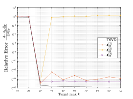
Figure 1: Tests for different implementations of the CURCA. We recommend the third implementation.


The results are depicted in Figure 1. First, we notice that the third implementation, $\mathtt{A_{IJ}^{(3)}}$, which is the one we suggest, yields stable approximation throughout the experiment. On the other hand, the second implementation, $\mathtt{A_{IJ}^{(2)}}$ suffers from numerical errors as we lose all accuracy past the target rank $30$. The reason is because we explicitly form the pseudoinverse of the core matrix $A(I,J)$, which is highly ill-conditioned, an observation also noted in [40]. Therefore, it is important to not form the pseudoinverse of $U=A(I,J)$ explicitly in the CURCA. Note also that the order in which the factors are multiplied is essential for numerical stability, as the second and third implementations only differ by the order in which the factors are computed. The first implementation, $\mathtt{A_{IJ}^{(1)}}$ may lose $1$ or $2$ orders of magnitude once the target rank becomes larger than $\operatorname{rank}(A)=30$ and appear to be less stable than the third implementation. The slash commands $(\mathtt{/,\backslash})$ in MATLAB should be used with caution for underdetermined problems, as its backslash command applied to numerically rank-deficient underdetermined problems output a sparse solution based on a pivoting strategy [2, § 2.4], which can differ significantly from the minimum-norm solution and may not satisfy the assumptions in our analysis.
Note that using the $\mathtt{pinv}$ command with tolerance parameter $0$ for the CURCA in MATLAB, i.e., $\mathtt{A(:,J)*pinv(A(I,J),0),*A(I,:)}$, is equivalent to the second implementation, which can be unstable. For the rest of the numerical experiments, we use the third implementation



(21)

$$\mathtt{\left(A(:,J)*V/S\right)*\left(W^{\prime}*A(I,:)\right)}\text{ where }\mathtt{[W,S,V]=svd(U,`econ^{\prime})}.$$





The stabilized CURCA can be implemented in such a way that the analysis in Section 2.2 hold. One approach is to take the SVD of $A(I,J)$ and truncate the singular values that are less than $\epsilon$ and form the SCURCA by using the third implementation, $\mathtt{A_{IJ}^{(3)}}$ with the truncated singular vectors and singular values. This implementation is reliable and require $\mathcal{O}(k^{3})$ operations. A less expensive alternative is to use a rank-revealing QR factorization and truncate the bottom-right corner of the upper triangular factor and the relevant columns of the orthonormal factor corresponding to the diagonal elements less than $\epsilon$. In the rank-revealing QR, the diagonal elements give a good approximation to the singular values; see for example [10, 27]. A possible workaround without the $\epsilon$-pseudoinverse is also discussed in [40] where we perturb the core matrix $A(I,J)$ by a small noise matrix such that the singular values of $A(I,J)$ are all larger than the unit roundoff.




4.2 Importance of not choosing rows and columns independently


In this section, we demonstrate the importance of choosing the rows and columns that are dependent on one another in the CURCA. If the rows and columns are chosen independently of each other, the matrix $U=A(I,J)$ can be (nearly) singular. In such a scenario, we show that a sufficient amount of oversampling can remedy this problem. We use the following synthetic test matrix:




$$A=\begin{bmatrix}10^{-10}\cdot\mathtt{randn(50,50)}&\mathtt{randn(50,950)}\\
\mathtt{randn(950,50)}&0\end{bmatrix}\in\mathbb{R}^{1000\times 1000}.$$



The matrix $A$ is generated randomly with $\operatorname{rank}(A)=100$ and has a small component in the $(1,1)$-block, a zero component in $(2,2)$-block and large components in the $(2,1)$- and $(1,2)$-blocks. We test the following four cases:


 

Choose columns and rows independently by applying CPQR on $A$ and $A^{T}$ respectively,



 

Choose columns and rows dependently by applying CPQR on $A$ and then applying CPQR on the chosen columns $A(:,J)$ to obtain the rows,



 

Apply Case $1$ and additionally do
row oversampling using Algorithm 2 with $p=k$,



 

Apply Case $2$ and additionally do row oversampling using Algorithm 2 with $p=k$,



where $k$ is the target rank.


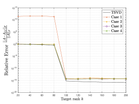
Figure 2: Relationship between the rows and columns in the CURCA. In Case $1$, the rows and columns are chosen independently from one another and in Case $2$, we select the columns first and then the rows were computed from the selected columns. Cases $3$ and $4$ correspond to Cases $1$ and $2$ with row oversampling ($p=k$), respectively.


In Figure 2, we show the importance of choosing the columns and rows in the CURCA. When the columns and rows are chosen independently (Case $1$), the resulting CURCA can be inaccurate before the target rank becomes large enough. This is because when we choose the columns and rows independently, we choose the first 50 rows and columns, as they are the most important, implying that the core matrix is the small $(1,1)$-block of $A$. Since the chosen rows and columns are $\mathcal{O}(1)$ and their intersection is $\mathcal{O}(10^{-10})$, the CURCA becomes inaccurate. A similar observation has also been made in the $2\times 2$ example at the end of Section 2.1. However, when we oversample sufficiently in Case $3$, we obtain a good CUR approximation. When we choose the rows and columns dependently in Cases $2$ and $4$, we have good stable approximations. Therefore, it is highly recommended to choose the rows and columns dependently. However, if that is not possible, a sufficient amount of oversampling is recommended.




4.3 Oversampling algorithm comparison


In this section, we illustrate advantages of oversampling through numerical experiments. In all experiments, unless stated otherwise, we use pivoting on a random sketch (Algorithm 1)
with column pivoted QR [19, 52] and the Gaussian sketch to get the initial set of $k$ row and column indices, where $k$ is the target rank. We then obtain the oversampling indices using the following algorithms:


 

$\mathtt{OS+P}$: Algorithm 2,



 

$\mathtt{OS+L}$: Choose $p$ extra indices corresponding to the largest $p$ leverage scores out of the unchosen indices as in [24],



 

$\mathtt{OS+E}$: $\mathtt{GappyPOD+E}$ algorithm in [45].



We set the number of oversampling indices to be $p=0$, $p=10$ and $p=0.5k$.


We consider three different classes of test matrices, which are summarized below:


 

$\mathtt{CIFAR10}$: The CIFAR-10 training set [35] consists of $60000$ images of size $32\times 32\times 3$. We choose $10000$ random images, each flattened to a vector, and treat it as a $10000\times 3072$ data matrix.



 

$\mathtt{YaleFace64x64}$: Yale face is a full-rank dense matrix of size $165\times 4096$ consisting of $165$ face images each of size $64\times 64$. The flattened image vectors are centered and normalized such that the mean is zero and the entries lie within $[-1,1]$.



 

$\mathtt{SNN}$: Random sparse non-negative matrices are test matrices used in [47, 52] that is given by,




$$\mathtt{SNN}=\sum_{j=1}^{r}s_{j}x_{j}y_{j}^{T},$$



where $s_{1}\geq\cdots\geq s_{r}>0$ and $x_{j}\in\mathbb{R}^{m},y_{j}\in\mathbb{R}^{n}$ are random sparse vectors with non-negative entries. We take $m=100000,n=300$ with




$$\sum_{j=1}^{50}\frac{2}{j}x_{j}y_{j}^{T}+\sum_{j=51}^{300}\frac{1}{j}x_{j}y_{j}^{T},$$



where the sparse vectors $x_{j}$’s and $y_{j}$’s are computed in MATLAB using the command $\mathtt{sprand}(m,1,0.025)$ and $\mathtt{sprand}(n,1,0.025)$, respectively.








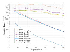
(a) CIFAR10 dataset with pivoting on a random sketch with row oversampling.




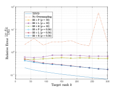
(b) CIFAR10 dataset with uniform sampling with row oversampling.





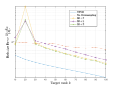
(c) YaleFace64x64 dataset with pivoting on a random sketch with row ($p=0.5k$) and column ($p=10$) oversampling.




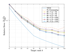
(d) SNN dataset with pivoting on a random sketch with row oversampling



Figure 3: Comparison of different oversampling methods for various test matrices. We use pivoting on a random sketch to obtain the initial set of indices except for Figure 3b where we use uniform sampling. Then we oversample the row indices using the three oversampling algorithms, $\mathtt{OS\!+\!P}$, $\mathtt{OS\!+\!L}$ and $\mathtt{OS\!+\!E}$. We also oversample column indices in Figure 3c.


The results are depicted in Figure 3. We compare different oversampling algorithms for the three test matrices. We use pivoting on a random sketch (Algorithm 1) to obtain the initial set of indices except for Figure 3b where we use uniform sampling; pivoting on a random sketch usually results in a good set of indices, while uniform sampling can give a poor set of indices. Then we oversample the row indices using the three oversampling algorithms, $\mathtt{OS\!+\!P}$, $\mathtt{OS\!+\!L}$ and $\mathtt{OS\!+\!E}$. We also oversample column indices in Figure 3c. For Figure 3c, $p=0.5k$ for row oversampling and $p=10$ for column oversampling.


We begin with the top two plots involving the CIFAR10 dataset, Figures 3a and 3b. We observe that as the oversampling parameter increases, the accuracy improves. The different oversampling techniques yield a similar result with $\mathtt{OS\!+\!L}$ being usually slightly worse. In Figures 3a and 3b, we observe that oversampling plays a big role for the accuracy of the CURCA. In Figure 3a, $p=10$ improves the accuracy slightly, but when the oversampling parameter $p$ becomes proportional to the target rank, we make further progress and we approximately capture the singular value decay rate. In Figure 3b, when the initial set of indices are worse, as it can be when we perform uniform sampling, we observe that oversampling makes the approximation more robust even when the CURCA without oversampling yields unstable results. Therefore, oversampling helps the CURCA yield more accurate and stable results.


In Figure 3c, using the YaleFace64x64 dataset, we show what happens when we oversample both row and column indices. In this experiment, we oversample the row indices by $p=0.5k$ and the column indices by $p=10$. In Figure 3c, the CURCA can get worse with oversampling and the approximation may become unstable when both column and row indices are oversampled. This is caused by the core matrix $A(I\cup I_{0},J\cup J_{0})$ underestimating the singular values of $A$ as oversampling in only one of row or column indices improve the condition number of the core matrix, but when we oversample both row and column indices, condition number of the core matrix can become worse. This is similar to the phenomenon happening in Section 4.2, where the CURCA can yield poor accuracy when we choose the rows and columns independently. Therefore, we advocate oversampling in only one of row or column indices for the CURCA. In Figure 3d, we use the $\mathtt{SNN}$ dataset. The effect of oversampling is less immediate in this example, but the accuracy still improves and we are less likely to see unstable approximation as we see in the no oversampling case near target rank $90$ and $100$ in Figure 3d.


Lastly, in all the experiments in Figure 3, we observe that our algorithm for oversampling $\mathtt{OS+P}$ (Algorithm 2) is competitive with $\mathtt{OS+E}$ with $\mathtt{OS+L}$ usually being slightly worse. Therefore, Algorithm 2, which runs with complexity $\mathcal{O}(nk^{2}+nkp)$ is competitive with $\mathtt{OS\!+\!E}$, which run with complexity $\mathcal{O}(nk^{2}p+k^{4})$.



5 Conclusion


In this work, we study the accuracy and stability of the CUR decomposition with oversampling. We prove the relative norm bounds for the CUR decomposition, $A\approx CU^{\dagger}R$, and its stabilized version, $A\approx CU_{\epsilon}^{\dagger}R$. We further show that the stabilized version satisfies a similar relative norm bound in the presence of roundoff errors under the assumption that the rows and columns for the CUR decomposition are chosen reasonably. This means that the rows should be selected based on the chosen columns or vice versa; see Section 4.2. This aims to reduce the quantity $\left\lVert Q_{C}(I,:)^{-1}\right\rVert_{2}$ (see Theorem 2.11), which can be further reduced by oversampling the row indices. For a stable implementation of the CURCA, $A\approx CU^{\dagger}R$, we recommend the MATLAB implementation




$$\mathtt{A_{IJ}^{(3)}=\left(A(:,J)*V/S\right)*\left(W^{\prime}*A(I,:)\right)}\text{ where }\mathtt{[W,S,V]=svd(U,`econ^{\prime})}$$



or the corresponding version where QR factorization is used instead of the SVD.


We also proposed how oversampling should be done. Oversampling should be done such that it increase the minimum singular value of a certain square matrix that is a submatrix of an orthonormal matrix; see Section 3. We suggest doing so through projecting the unchosen rows of an orthonormal matrix onto the trailing singular subspace of the square matrix and finding the important unchosen indices that will enrich the trailing singular subspace; see Algorithm 2. Oversampling improves the stability as the core matrix becomes rectangular and rectangular matrices are more well-conditioned than square matrices. We recommend oversampling in one only one of row or column indices, but not both (see Figure 3c) and choose the oversampling parameter to be proportional to the target rank when possible. Experiments show that the algorithm is competitive with other existing methods. Therefore, we advocate oversampling for the accuracy and stability of the CUR decomposition whenever possible.




Appendix A Analysis of the CURBA


In this section, we analyze the CURBA,



(22)

$$A_{IJ}^{(BA)}=A(:,J)\left(A(:,J)^{\dagger}AA(I,:)^{\dagger}\right)A(I,:)=C(C^{\dagger}AR^{\dagger})R$$



with oversampling. For the CURBA, there exists a numerically stable algorthm given by the StableCUR algorithm in [1]. The algorithm computes the CURBA in the following way in MATLAB,



(23)

$$\mathtt{[Q_{C},\sim]=qr(A(:,J),0)},\;\mathtt{[Q_{R},\sim]=qr(A(I,:)^{\prime},0)},\;A_{IJ}^{(BA)}=\mathtt{Q_{C}*(Q_{C}^{\prime}*A*Q_{R})*Q_{R}^{\prime}}.$$



We use this implementation of the CURBA in the experiments at the end of this section.


We first prove a relative norm bound for the CURBA with oversampling. We make the following standard assumptions, which is analogous to the CURCA counterpart in Section 2.
  ⁢


 

$|I|=|J|=k$ where $k$ is the target rank. The oversampling indices are $I_{0}$ with $|I_{0}|=p_{1}$ for the rows and $J_{0}$ with $|J_{0}|=p_{2}$ for the columns and they satisfy $k+\max\{p_{1},p_{2}\}\leq\operatorname{rank}(A)$.



 

$A(:,J\cup J_{0})$ has full column rank and $A(I\cup I_{0},:)$ has full row rank.



 

$X(:,J)\in\mathbb{R}^{k\times(k+p_{2})}$ has full row rank, where $X\in\mathbb{R}^{k\times n}$ is a row space approximator of $A$.



 

$Y(I,:)\in\mathbb{R}^{k\times(k+p_{2})}$ has full row rank, where $Y\in\mathbb{R}^{m\times k}$ is a column space approximator of $A$.



The assumption that $X(:,J)$ and $A(I,:)$ having a full row rank and $Y(I,:)$ and $A(:,J)$ having a full column rank is generic, since most methods that pick good row and column indices satisfy this assumption. If one of $X$ or $Y$ are not available then $A(I,:)$ or $A(:,J)$ can be used instead, respectively.


We now prove the result for the CURBA with oversampling. The results shown below is a simple extension of [47, Lemma 4.2] and [19, Theorem 1]. Lemma A.1 considers one-sided projection with oversampling where we project $A$ onto the chosen columns of $A$. In Theorem A.3, we consider the CURBA, $C(C^{\dagger}AR^{\dagger})R$ where we project $A$ onto the chosen rows and columns of $A$.



Lemma A.1.


Under Assumption A,



(24)

$$\left\lVert A-CC^{\dagger}A\right\rVert\leq\left\lVert Q_{X}(J\cup J_{0},:)^{\dagger}\right\rVert_{2}\left\lVert A-AX^{\dagger}X\right\rVert$$



where $\left\lVert\cdot\right\rVert$ is any unitarily invariant norm and $Q_{X}\in\mathbb{R}^{n\times k}$ is an orthonormal matrix spanning the columns of $X^{T}$.





Proof A.2.


For shorthand let $J_{*}=J\cup J_{0}$ and let $\Pi_{J_{*}}=I_{n}(:,J_{*})\in\mathbb{R}^{n\times(k+p)}$ such that $C=A(:,J_{*})=A\Pi_{J_{*}}$. We first define two oblique projectors




$$\mathcal{P}_{X}:=\Pi_{J_{*}}(X\Pi_{J_{*}})^{\dagger}X,\hskip 14.22636pt\mathcal{P}_{C}:=\Pi_{J_{*}}C^{\dagger}A\in\mathbb{R}^{n\times n}.$$



Note that since $C$ has full column rank, $C^{\dagger}A\Pi_{J_{*}}=C^{\dagger}C=I_{k+p}$, and




$$\mathcal{P}_{C}\mathcal{P}_{X}=\Pi_{J_{*}}C^{\dagger}A\Pi_{J_{*}}(X\Pi_{J_{*}})^{\dagger}X=\mathcal{P}_{X}.$$



Therefore we get




$$A-CC^{\dagger}A=A(I-\mathcal{P}_{C})=A(I-\mathcal{P}_{C})(I-\mathcal{P}_{X})=(I-CC^{\dagger})A(I-\mathcal{P}_{X}).$$



Since $X\Pi_{J_{*}}=X(:,J_{*})$ has full row rank,




$$X\mathcal{P}_{X}=X\Pi_{J_{*}}\left(X\Pi_{J_{*}}\right)^{\dagger}X=X$$



and we obtain




$$(I-\mathcal{P}_{X})=(I-X^{\dagger}X)(I-\mathcal{P}_{X}).$$



Now putting these together, we obtain




$$\left\lVert A-CC^{\dagger}A\right\rVert
=\left\lVert(I-CC^{\dagger})A(I-X^{\dagger}X)(I-\mathcal{P}_{X})\right\rVert$$






$$\leq\left\lVert I-CC^{\dagger}\right\rVert_{2}\left\lVert A(I-X^{\dagger}X)\right\rVert\left\lVert I-\mathcal{P}_{X}\right\rVert_{2}$$





$$=\left\lVert I-\mathcal{P}_{X}\right\rVert_{2}\left\lVert A(I-X^{\dagger}X)\right\rVert,$$



since $\left\lVert I-CC^{\dagger}\right\rVert_{2}=1$ as $CC^{\dagger}$ is an orthogonal projector. Now since $\mathcal{P}_{X}$ is an oblique projector [48], $\left\lVert I-\mathcal{P}_{X}\right\rVert_{2}=\left\lVert\mathcal{P}_{X}\right\rVert_{2}$ so the result follows by noting that




$$\left\lVert\mathcal{P}_{X}\right\rVert_{2}=\left\lVert(X\Pi_{J})^{\dagger}X\right\rVert_{2}=\left\lVert Q_{X}(J,:)\right\rVert_{2}.$$








Theorem A.3.


Under Assumption A,



(25)

$$\left\lVert A-A_{I\cup I_{0},J\cup J_{0}}^{(BA)}\right\rVert
\leq\left\lVert Q_{X}(J\cup J_{0},:)^{\dagger}\right\rVert_{2}\left\lVert A-AX^{\dagger}X\right\rVert$$






$$\hskip 28.45274pt+\left\lVert Q_{Y}(I\cup I_{0},:)^{\dagger}\right\rVert_{2}\left\lVert A-YY^{\dagger}A\right\rVert$$



where $\left\lVert\cdot\right\rVert$ is any unitarily invariant norm and $Q_{X}\in\mathbb{R}^{n\times k}$ and $Q_{Y}\in\mathbb{R}^{m\times k}$ are the orthonormal matrices spanning the columns of $X^{T}$ and $Y$, respectively.





Proof A.4.


The proof follows by Lemma A.1 and noting that




$$\left\lVert A-CC^{\dagger}AR^{\dagger}R\right\rVert
\leq\left\lVert A-CC^{\dagger}A\right\rVert+\left\lVert CC^{\dagger}A-CC^{\dagger}AR^{\dagger}R\right\rVert$$






$$\leq\left\lVert A-CC^{\dagger}A\right\rVert+\left\lVert CC^{\dagger}\right\rVert_{2}\left\lVert A-AR^{\dagger}R\right\rVert$$





$$=\left\lVert A-CC^{\dagger}A\right\rVert+\left\lVert A-AR^{\dagger}R\right\rVert$$





$$\leq\left\lVert Q_{X}(J,:)^{\dagger}\right\rVert_{2}\left\lVert A-AX^{\dagger}X\right\rVert+\left\lVert Q_{Y}(I,:)^{\dagger}\right\rVert_{2}\left\lVert A-YY^{\dagger}A\right\rVert$$



where the inequality for the second term $\left\lVert A-AR^{\dagger}R\right\rVert$ in the final line can be shown by considering $A^{T}$ in Lemma A.1.





Remark A.5.





 

The difference between Theorem A.3 and its counterpart without oversampling, e.g. [19, Theorem 1], are the terms $\left\lVert Q_{X}(J,:)^{\dagger}\right\rVert_{2}$ and $\left\lVert Q_{Y}(I,:)^{\dagger}\right\rVert_{2}$ where instead of the matrix inverse, we have the pseudoinverse. This tightens the bound (25) as




$$\left\lVert Q_{X}(J\cup J_{0},:)^{\dagger}\right\rVert_{2}\leq\left\lVert Q_{X}(J,:)^{-1}\right\rVert_{2},$$



and




$$\left\lVert Q_{Y}(I\cup I_{0},:)^{\dagger}\right\rVert_{2}\leq\left\lVert Q_{Y}(I,:)^{-1}\right\rVert_{2},$$



where $I_{0}$ and $J_{0}$ are the extra indices for oversampling.



 

There are many possible choices for $X$ and $Y$. For example, if we choose them to be the dominant right and left singular vectors of $A$, then we get the bound similar to the one in [47] involving the best rank-$k$ approximation since $\left\lVert A-AX^{\dagger}X\right\rVert=\left\lVert A-YY^{\dagger}A\right\rVert=\left\lVert A-\llbracket{A}\rrbracket_{k}\right\rVert$ where $\llbracket{A}\rrbracket_{k}$ is the best rank-$k$ approximation to $A$. If we choose $X$ and $Y$ to be the row sketch and the column sketch (see Algorithm 1) then we involve the randomized SVD error [28]. Choosing $X$ and $Y$ to be the dominant singular vectors in Theorem A.3 can be the optimal choice, but when $X$ and $Y$ are approximators, which can be computed easily, the bound (25) can be computed a posteriori.



 

When $k+\min\{p_{1},p_{2}\}\geq\operatorname{rank}(A)$ and $\operatorname{rank}(C)=\operatorname{rank}(R)=\operatorname{rank}(A)$, we have $A=CC^{\dagger}AR^{\dagger}R$ [29].







Theorem A.3 suggests that oversampling helps to improve the accuracy of the CUR decomposition $A_{IJ}^{(BA)}$. However, the numerical simulations shown below illustrate that the improvement is not too significant.





(a) CIFAR10 dataset with pivoting on a random sketch with row oversampling.




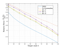
(b) YaleFace64x64 dataset with pivoting on a random sketch with row $(p=0.5k)$ oversampling and column $(p=10)$ oversampling.



Figure 4: The effect of oversampling for the CURBA. We use pivoting on a random sketch (Algorithm 1) to obtain the initial set of indices. Then we oversample the row indices using the three oversampling algorithms, $\mathtt{OS\!+\!P}$, $\mathtt{OS\!+\!L}$ and $\mathtt{OS\!+\!E}$. We also oversample column indices in Figure 4b.


The numerical results are depicted in Figure 4, illustrating the effect of oversampling for the CURBA. We use pivoting on a random sketch (Algorithm 1) to obtain the initial set of indices. Then we oversample the row indices using the three oversampling algorithms, $\mathtt{OS\!+\!P}$, $\mathtt{OS\!+\!L}$ and $\mathtt{OS\!+\!E}$ as in Section 4.3. We also oversample column indices in Figure 4b.


We start with the CIFAR10 dataset in Figure 4a. We first observe that as the oversampling parameter increases, the accuracy improves and the different oversampling techniques yield a similar result. However, there is no significant improvement when oversampling is used for the CURBA. This shows that the CURBA gives a robust approximation and oversampling only plays a slight role in its accuracy. In Figure 4b, we used the YaleFace64x64 dataset to illustrate the effect of oversampling both rows and columns. We observe that when we oversample both rows and columns, we obtain a higher accuracy for the CURBA. This is expected as we are enlarging the subspace that we project onto $A$, which increases the accuracy of the CURBA. This is contrary to the CURCA, as the CURCA can become more inaccurate and unstable when we oversample both rows and columns; see Section 4.3.


To conclude, while oversampling improves the accuracy of the CURBA, it has less significant effect on its accuracy and stability.




Appendix B Stability of rank-deficient systems


In this section, we prove the stability result for solving rank-deficient underdetermined linear systems (Theorem 2.10). The result can also be extended to rank-deficient overdetermined problems; see Appendix B.1. Theorem 2.10 was used to derive an expression for the computed solution to



(26)

$$\min_{x}\left\lVert(\hat{U}^{T})_{\epsilon}x-[\hat{C}]_{i}^{T}\right\rVert_{2}$$



for each row of $\hat{C}$. The statement and the proof is shown below. The proof follows a similar method outlined in [40, Section 4.1].



Theorem B.1 (Theorem 2.10).


Consider the (rank-deficient) underdetermined linear system,



(9)

$$\min_{x^{\prime}}\left\lVert B_{\epsilon}x^{\prime}-b\right\rVert_{2}$$



where $B_{\epsilon}\in\mathbb{R}^{m\times n}$ $(m\leq n)$ is (possibly) rank-deficient $(\operatorname{rank}(B_{\epsilon})\leq m)$ with singular vales larger than $\epsilon$ and $b\in\mathbb{R}^{m}$. Then assuming $\epsilon>\gamma\left\lVert B_{\epsilon}\right\rVert_{2}$, the minimum norm solution to (9) can be computed in a backward stable manner, i.e., the computed solution $\hat{s}$ satisfies




$$\hat{s}=\left(B_{\epsilon}+E_{1}\right)^{\dagger}\left(b+E_{2}\right)$$



where $\left\lVert E_{1}\right\rVert_{2}\leq\gamma\left\lVert B_{\epsilon}\right\rVert_{2}$ and $\left\lVert E_{2}\right\rVert_{2}\leq\gamma\left\lVert b\right\rVert_{2}$.





Proof B.2.


First, if $B_{\epsilon}$ has full row-rank then the statement follows by the stability result in [32, Theorem 21.4]. If $B_{\epsilon}$ is rank-deficient,
the stability result in [32, Theorem 21.4] cannot be invoked as it is only applicable for underdetermined full-rank linear systems. So we project $B_{\epsilon}$ onto its column space $Q_{\epsilon}$ to make the problem an underdetermined full-rank linear system:




$$\min_{x^{\prime}}\left\lVert Q_{\epsilon}^{T}B_{\epsilon}x^{\prime}-Q_{\epsilon}^{T}b\right\rVert_{2}.$$





Let $\hat{Q}_{\epsilon}$ be the computed column space of $B_{\epsilon}$. Then $\hat{Q}_{\epsilon}$ is the exact column space of $B_{\epsilon}+\Delta B$ where $\left\lVert\Delta B\right\rVert_{2}\leq\gamma\left\lVert B_{\epsilon}\right\rVert_{2}$, $\hat{Q}_{\epsilon}^{T}B_{\epsilon}$ is numerically full-rank with singular values larger than $\epsilon$ and $\hat{Q}_{\epsilon}\hat{Q}_{\epsilon}^{T}B_{\epsilon}=B_{\epsilon}+E$ where $\left\lVert E\right\rVert_{2}\leq\gamma\left\lVert B_{\epsilon}\right\rVert_{2}$ [25, Chapter 5.4.1]. Note the following from matrix-matrix (or matrix-vector) multiplication [32, Section 3.5],




$$fl(\hat{Q}_{\epsilon}^{T}B_{\epsilon})=\hat{Q}_{\epsilon}^{T}B_{\epsilon}+E^{(1)}$$



where $\left\lVert E^{(1)}\right\rVert_{2}\leq\gamma\left\lVert B_{\epsilon}\right\rVert_{2}$ and




$$fl(\hat{Q}_{\epsilon}^{T}b)=\hat{Q}_{\epsilon}^{T}b+E^{(2)}$$



where $\left\lVert E^{(2)}\right\rVert_{2}\leq\gamma\left\lVert b\right\rVert_{2}$. Since $\hat{Q_{\epsilon}^{T}B_{\epsilon}}\in\mathbb{R}^{\operatorname{rank}(B_{\epsilon})\times n}$ is a fat rectangular matrix, we solve the following underdetermined full-rank linear system,



(27)

$$\min_{x^{\prime}}\left\lVert(\hat{Q}_{\epsilon}^{T}B_{\epsilon})x^{\prime}-\hat{Q}_{\epsilon}^{T}b\right\rVert_{2}.$$



Assuming $\gamma\kappa_{2}(B_{\epsilon})\leq\gamma\left\lVert B_{\epsilon}\right\rVert_{2}/\epsilon<1$ (where $\kappa_{2}$ denotes the 2-norm condition number), we obtain the computed solution of (27), $\hat{s}$, satisfying [32, Theorem 21.4],




$$\hat{s}=fl\left(\left(\hat{Q}_{\epsilon}^{T}B_{\epsilon}\right)^{\dagger}\hat{Q}_{\epsilon}^{T}b\right)
=\left(fl(\hat{Q}_{\epsilon}^{T}B_{\epsilon})+E^{(3)}\right)^{\dagger}fl(\hat{Q}_{\epsilon}^{T}b)$$






$$=\left(\hat{Q}_{\epsilon}^{T}B_{\epsilon}+E^{(1)}+E^{(3)}\right)^{\dagger}\left(\hat{Q}_{\epsilon}^{T}b+E^{(2)}\right)$$





$$=\left(\hat{Q}_{\epsilon}\hat{Q}_{\epsilon}^{T}B_{\epsilon}+\hat{Q}_{\epsilon}E^{(1)}+\hat{Q}_{\epsilon}E^{(3)}\right)^{\dagger}\left(b+\hat{Q}_{\epsilon}E^{(2)}\right)$$





$$=\left(B_{\epsilon}+E+\hat{Q}_{\epsilon}E^{(1)}+\hat{Q}_{\epsilon}E^{(3)}\right)^{\dagger}\left(b+\hat{Q}_{\epsilon}E^{(2)}\right)$$



where $\left\lVert E^{(3)}\right\rVert_{2}\leq\gamma\left\lVert B_{\epsilon}\right\rVert_{2}$ and we use $(QA)^{\dagger}b=A^{\dagger}Q^{T}b$ for a tall-skinny orthonormal matrix $Q$ in line $3$. Therefore, assuming that $\gamma\left\lVert B_{\epsilon}\right\rVert_{2}<\epsilon$, the computed solution of (9), $\hat{s}$ satisfies



(28)

$$\hat{s}=fl(B_{\epsilon}^{\dagger}b)=\left(B_{\epsilon}+E_{1}\right)^{\dagger}\left(b+E_{2}\right),$$



where $\left\lVert E_{1}\right\rVert_{2}\leq\gamma\left\lVert B_{\epsilon}\right\rVert_{2}$ and $\left\lVert E_{2}\right\rVert_{2}\leq\gamma\left\lVert b\right\rVert_{2}$.





B.1 Extension to rank-deficient overdetermined problems


Theorem 2.10 can be extended to include rank-deficient overdetermined least-sqaures problems. Consider the rank-deficient overdetermined least-squares problem,




$$\min_{x^{\prime}}\left\lVert C_{\epsilon}x^{\prime}-b\right\rVert_{2}$$



where $C_{\epsilon}\in\mathbb{R}^{m\times n}$ $(m\geq n)$ is a rank-deficient $(\operatorname{rank}(C_{\epsilon})<n)$, tall-skinny matrix with singular vales larger than $\epsilon$ and $b\in\mathbb{R}^{m}$. Then under the same assumption as Theorem 2.10, i.e., $\epsilon>\gamma\left\lVert B_{\epsilon}\right\rVert_{2}$, the solution to the overdetermined least-squares problem can be computed in a backward stable manner.


The proof proceeds in the same way as Theorem 2.10, as once the tall-skinny matrix $C_{\epsilon}$ is projected onto its column space $W_{\epsilon}$, $W_{\epsilon}^{T}C_{\epsilon}\in\mathbb{R}^{\operatorname{rank}(C_{\epsilon})\times n}$ becomes a fat full-rank matrix, and we are now solving the underdetermined full-rank linear system: $\min\limits_{x^{\prime}}\left\lVert(\hat{W}_{\epsilon}^{T}C_{\epsilon})x^{\prime}-\hat{W}_{\epsilon}^{T}b\right\rVert_{2}$.





Appendix C Two lemmas


We give the proofs for the two lemmas, Lemma 2.8 and Lemma 2.9 in this section.



Lemma C.1 (Lemma 2.8).


Under Assumption 2.2, for any $\Delta C$ and $\Delta U$,



(29)

$$\left\lVert(C+\Delta C)(U+\Delta U)_{\epsilon}^{\dagger}\right\rVert_{2}\leq\left\lVert Q_{C}(I_{*},:)^{\dagger}\right\rVert_{2}\left(1+\frac{1}{\epsilon}\left\lVert\Delta U\right\rVert_{2}\right)+\frac{1}{\epsilon}\left\lVert\Delta C\right\rVert_{2}.$$








Proof C.2.


Let $C=Q_{C}R_{C}$ be the thin QR factorization of $C$. Then




$$\left\lVert(C+\Delta C)(U+\Delta U)_{\epsilon}^{\dagger}\right\rVert_{2}
\leq\left\lVert Q_{C}R_{C}(U+\Delta U)_{\epsilon}^{\dagger}\right\rVert_{2}+\left\lVert\Delta C(U+\Delta U)_{\epsilon}^{\dagger}\right\rVert_{2}$$






$$=\left\lVert R_{C}(U+\Delta U)_{\epsilon}^{\dagger}\right\rVert_{2}+\left\lVert\Delta C(U+\Delta U)_{\epsilon}^{\dagger}\right\rVert_{2}$$





$$=\left\lVert(\Pi_{I_{*}}^{T}Q_{C})^{\dagger}\Pi_{I_{*}}^{T}Q_{C}R_{C}(U+\Delta U)_{\epsilon}^{\dagger}\right\rVert_{2}+\left\lVert\Delta C(U+\Delta U)_{\epsilon}^{\dagger}\right\rVert_{2}$$





$$\leq\left\lVert(\Pi_{I_{*}}^{T}Q_{C})^{\dagger}\right\rVert_{2}\left\lVert U(U+\Delta U)_{\epsilon}^{\dagger}\right\rVert_{2}+\frac{1}{\epsilon}\left\lVert\Delta C\right\rVert_{2}$$



where we use $(\Pi_{I_{*}}^{T}Q_{C})^{\dagger}\Pi_{I_{*}}^{T}Q_{C}=I$ for the penultimate line.
The result follows by noting that $\left\lVert U(U+\Delta U)_{\epsilon}^{\dagger}\right\rVert_{2}$ simplifies to




$$\left\lVert U(U+\Delta U)_{\epsilon}^{\dagger}\right\rVert_{2}=\left\lVert(U+\Delta U)(U+\Delta U)_{\epsilon}^{\dagger}-\Delta U(U+\Delta U)_{\epsilon}^{\dagger}\right\rVert_{2}\leq 1+\frac{1}{\epsilon}\left\lVert\Delta U\right\rVert_{2}.$$








Lemma C.3 (Lemma 2.9).


Under Assumption 2.2, for any $\Delta C$ and $\Delta U$,



(30)

$$(C+\Delta C)(U+\Delta U)_{\epsilon}^{\dagger}R\Pi_{J}=C+E_{*}$$



where




$$\left\lVert E_{*}\right\rVert_{2}\leq\left\lVert(Q_{C}(I_{*},:)^{\dagger}\right\rVert_{2}\left(\epsilon+2\left\lVert\Delta U\right\rVert_{2}+\frac{1}{\epsilon}\left\lVert\Delta U\right\rVert_{2}^{2}\right)+\left\lVert\Delta C\right\rVert_{2}\left(1+\frac{\left\lVert\Delta U\right\rVert_{2}}{\epsilon}\right).$$








Proof C.4.


We divide the expression into two pieces:




$$(C+\Delta C)(U+\Delta U)_{\epsilon}^{\dagger}R\Pi_{J}=\underbrace{C(U+\Delta U)_{\epsilon}^{\dagger}R\Pi_{J}}_{(i)}+\underbrace{\Delta C(U+\Delta U)_{\epsilon}^{\dagger}R\Pi_{J}}_{(ii)}$$



and treat them separately. Let the thin SVD of $U+\Delta U$ be




$$U+\Delta U=W\Sigma V^{T}=[W_{1},W_{2}]\begin{bmatrix}\Sigma_{1}&\\
&\Sigma_{2}\end{bmatrix}[V_{1},V_{2}]^{T}$$



where $\Sigma_{2}$ contains the singular values of $U+\Delta U$ smaller than $\epsilon$ and $C=Q_{C}R_{C}$ be the thin QR decomposition of $C$.


We begin by examining the matrix (i).




$$C(U+\Delta U)_{\epsilon}^{\dagger}R\Pi_{J}
=C(U+\Delta U)_{\epsilon}^{\dagger}U=C(U+\Delta U)_{\epsilon}^{\dagger}(U+\Delta U)-C(U+\Delta U)_{\epsilon}^{\dagger}\Delta U$$






$$=CV_{1}V_{1}^{T}-C(U+\Delta U)_{\epsilon}^{\dagger}\Delta U=C-CV_{2}V_{2}^{T}-C(U+\Delta U)_{\epsilon}^{\dagger}\Delta U$$





$$=C+E_{1}$$



where $E_{1}=-CV_{2}V_{2}^{T}-C(U+\Delta U)_{\epsilon}^{\dagger}\Delta U$ satisfies




$$\left\lVert E_{1}\right\rVert_{2}
\leq\left\lVert CV_{2}V_{2}^{T}\right\rVert_{2}+\left\lVert C(U+\Delta U)_{\epsilon}^{\dagger}\Delta U\right\rVert_{2}$$






$$\leq\left\lVert CV_{2}V_{2}^{T}\right\rVert_{2}+\left\lVert Q_{C}(I_{*},:)^{\dagger}\right\rVert_{2}\left(1+\frac{1}{\epsilon}\left\lVert\Delta U\right\rVert\right)\left\lVert\Delta U\right\rVert_{2}$$



by Lemma 2.8. We bound $\left\lVert CV_{2}V_{2}^{T}\right\rVert_{2}$ as in the final part of the proof of Theorem 2.3.




$$\left\lVert CV_{2}V_{2}^{T}\right\rVert_{2}
=\left\lVert R_{C}V_{2}V_{2}^{T}\right\rVert_{2}=\left\lVert(\Pi_{I_{*}}^{T}Q_{C})^{\dagger}\Pi_{I_{*}}^{T}Q_{C}R_{C}V_{2}V_{2}^{T}\right\rVert_{2}=\left\lVert(\Pi_{I_{*}}^{T}Q_{C})^{\dagger}UV_{2}V_{2}^{T}\right\rVert_{2}$$






$$\leq\left\lVert(\Pi_{I_{*}}^{T}Q_{C})^{\dagger}\right\rVert_{2}\left\lVert(U+\Delta U)V_{2}V_{2}^{T}-\Delta UV_{2}V_{2}^{T}\right\rVert_{2}$$





$$\leq\left\lVert(\Pi_{I_{*}}^{T}Q_{C})^{\dagger}\right\rVert_{2}\left(\left\lVert W_{2}\Sigma_{2}\right\rVert_{2}+\left\lVert\Delta U\right\rVert_{2}\right)$$





$$\leq\left\lVert(\Pi_{I_{*}}^{T}Q_{C})^{\dagger}\right\rVert_{2}\left(\epsilon+\left\lVert\Delta U\right\rVert_{2}\right).$$



Therefore, (i) can be bounded as




$$C(U+\Delta U)_{\epsilon}^{\dagger}R\Pi_{J}=C+E_{1}$$



where $\left\lVert E_{1}\right\rVert_{2}\leq\left\lVert(Q_{C}(I_{*},:)^{\dagger}\right\rVert_{2}\left(\epsilon+2\left\lVert\Delta U\right\rVert_{2}+\frac{1}{\epsilon}\left\lVert\Delta U\right\rVert_{2}^{2}\right)$.


Next, we bound the matrix (ii). Let $E_{2}=\Delta C(U+\Delta U)_{\epsilon}^{\dagger}R\Pi_{J}$, then




$$\left\lVert E_{2}\right\rVert_{2}
=\left\lVert\Delta C(U+\Delta U)_{\epsilon}^{\dagger}R\Pi_{J}\right\rVert_{2}$$






$$\leq\left\lVert\Delta C\right\rVert_{2}\left\lVert(U+\Delta U)_{\epsilon}^{\dagger}U\right\rVert_{2}$$





$$\leq\left\lVert\Delta C\right\rVert_{2}\left(\left\lVert(U+\Delta U)_{\epsilon}^{\dagger}(U+\Delta U)\right\rVert_{2}+\left\lVert(U+\Delta U)_{\epsilon}^{\dagger}\Delta U\right\rVert_{2}\right)$$





$$\leq\left\lVert\Delta C\right\rVert_{2}\left(1+\frac{\left\lVert\Delta U\right\rVert_{2}}{\epsilon}\right).$$





Putting everything together and setting $E_{*}=E_{1}+E_{2}$, we get the desired result:




$$(C+\Delta C)(U+\Delta U)_{\epsilon}^{\dagger}R\Pi_{J}=C+E_{*}$$



where




$$\left\lVert E_{*}\right\rVert_{2}\leq\left\lVert(Q_{C}(I_{*},:)^{\dagger}\right\rVert_{2}\left(\epsilon+2\left\lVert\Delta U\right\rVert_{2}+\frac{1}{\epsilon}\left\lVert\Delta U\right\rVert_{2}^{2}\right)+\left\lVert\Delta C\right\rVert_{2}\left(1+\frac{\left\lVert\Delta U\right\rVert_{2}}{\epsilon}\right).$$

References

• [1] D. Anderson, S. Du, M. Mahoney, C. Melgaard, K. Wu, and M. Gu, Spectral Gap Error Bounds for Improving CUR Matrix Decomposition and the Nyström Method, in Proceedings of the Eighteenth International Conference on Artificial Intelligence and Statistics, G. Lebanon and S. V. N. Vishwanathan, eds., vol. 38 of Proceedings of Machine Learning Research, San Diego, California, USA, 09–12 May 2015, PMLR, pp. 19–27.
• [2] E. Anderson, Z. Bai, C. Bischof, J. Demmel, J. Dongarra, J. Du Croz, A. Greenbaum, S. Hammarling, A. McKenney, S. Ostrouchov, et al., LAPACK Users’ guide, SIAM, 1995.
• [3] H. Avron, P. Maymounkov, and S. Toledo, Blendenpik: Supercharging LAPACK’s least-squares solver, SIAM J. Sci. Comput., 32 (2010), pp. 1217–1236, https://doi.org/10.1137/090767911.
• [4] O. Balabanov and L. Grigori, Randomized Gram–Schmidt process with application to GMRES, SIAM J. Sci. Comput., 44 (2022), pp. A1450–A1474, https://doi.org/10.1137/20M138870X.
• [5] J. Batson, D. A. Spielman, and N. Srivastava, Twice-ramanujan sparsifiers, SIAM J. Comput., 41 (2012), pp. 1704–1721, https://doi.org/10.1137/090772873.
• [6] C. Boutsidis, P. Drineas, and M. Magdon-Ismail, Near-optimal column-based matrix reconstruction, SIAM J. Comput., 43 (2014), pp. 687–717, https://doi.org/10.1137/12086755X.
• [7] C. Boutsidis and D. P. Woodruff, Optimal CUR matrix decompositions, SIAM J. Comput., 46 (2017), pp. 543–589, https://doi.org/10.1137/140977898.
• [8] D. Cai, J. Nagy, and Y. Xi, Fast deterministic approximation of symmetric indefinite kernel matrices with high dimensional datasets, SIAM J. Matrix Anal. Appl., 43 (2022), pp. 1003–1028, https://doi.org/10.1137/21M1424627.
• [9] K. Carlberg, C. Farhat, J. Cortial, and D. Amsallem, The GNAT method for nonlinear model reduction: Effective implementation and application to computational fluid dynamics and turbulent flows, J. Comput. Phys., 242 (2013), pp. 623–647, https://doi.org/https://doi.org/10.1016/j.jcp.2013.02.028.
• [10] T. F. Chan, Rank revealing QR factorizations, Linear Algebra Appl., 88-89 (1987), pp. 67–82, https://doi.org/https://doi.org/10.1016/0024-3795(87)90103-0.
• [11] S. Chaturantabut and D. C. Sorensen, Nonlinear model reduction via discrete empirical interpolation, SIAM J. Sci. Comput., 32 (2010), pp. 2737–2764, https://doi.org/10.1137/090766498.
• [12] J. Chiu and L. Demanet, Sublinear randomized algorithms for skeleton decompositions, SIAM J. Matrix Anal. Appl., 34 (2013), pp. 1361–1383, https://doi.org/10.1137/110852310.
• [13] A. Cortinovis and D. Kressner, Low-rank approximation in the Frobenius norm by column and row subset selection, SIAM J. Matrix Anal. Appl., 41 (2020), pp. 1651–1673.
• [14] A. Cortinovis and L. Ying, A sublinear-time randomized algorithm for column and row subset selection based on strong rank-revealing QR factorizations, arXiv preprint arXiv:2402.13975, (2024).
• [15] M. Dereziński and M. Mahoney, Determinantal point processes in randomized numerical linear algebra, Notices Amer. Math. Soc., 60 (2021), p. 1, https://doi.org/10.1090/noti2202.
• [16] A. Deshpande, L. Rademacher, S. S. Vempala, and G. Wang, Matrix approximation and projective clustering via volume sampling, Theory Comput., 2 (2006), pp. 225–247, https://doi.org/10.4086/toc.2006.v002a012.
• [17] A. Deshpande and S. Vempala, Adaptive sampling and fast low-rank matrix approximation, in Approximation, Randomization, and Combinatorial Optimization. Algorithms and Techniques, J. Díaz, K. Jansen, J. D. P. Rolim, and U. Zwick, eds., Berlin, Heidelberg, 2006, Springer Berlin Heidelberg, pp. 292–303.
• [18] M. Donello, G. Palkar, M. H. Naderi, D. C. Del Rey Fernández, and H. Babaee, Oblique projection for scalable rank-adaptive reduced-order modelling of nonlinear stochastic partial differential equations with time-dependent bases, Proceedings of the Royal Society A: Mathematical, Physical and Engineering Sciences, 479 (2023), p. 20230320, https://doi.org/10.1098/rspa.2023.0320.
• [19] Y. Dong and P.-G. Martinsson, Simpler is better: a comparative study of randomized pivoting algorithms for CUR and interpolative decompositions, Adv. Comput. Math., 49 (2023), https://doi.org/10.1007/s10444-023-10061-z.
• [20] P. Drineas, M. Magdon-Ismail, M. W. Mahoney, and D. P. Woodruff, Fast approximation of matrix coherence and statistical leverage, J. Mach. Learn. Res., 13 (2012), pp. 3475–3506, http://jmlr.org/papers/v13/drineas12a.html.
• [21] P. Drineas, M. W. Mahoney, and S. Muthukrishnan, Relative-error CUR matrix decompositions, SIAM J. Matrix Anal. Appl., 30 (2008), pp. 844–881, https://doi.org/10.1137/07070471X.
• [22] Z. Drmač and S. Gugercin, A new selection operator for the discrete empirical interpolation method—improved a priori error bound and extensions, SIAM J. Sci. Comput., 38 (2016), pp. A631–A648, https://doi.org/10.1137/15M1019271.
• [23] J. A. Duersch and M. Gu, Randomized projection for rank-revealing matrix factorizations and low-rank approximations, SIAM Rev., 62 (2020), pp. 661–682, https://doi.org/10.1137/20M1335571.
• [24] P. Y. Gidisu and M. E. Hochstenbach, A hybrid DEIM and leverage scores based method for CUR index selection, in Progress in Industrial Mathematics at ECMI 2021, M. Ehrhardt and M. Günther, eds., Cham, 2022, Springer International Publishing, pp. 147–153.
• [25] G. H. Golub and C. F. Van Loan, Matrix Computations, Johns Hopkins University Press, 4 ed., 2013.
• [26] S. Goreinov, E. Tyrtyshnikov, and N. Zamarashkin, A theory of pseudoskeleton approximations, Linear Algebra Appl., 261 (1997), pp. 1–21, https://doi.org/https://doi.org/10.1016/S0024-3795(96)00301-1.
• [27] M. Gu and S. C. Eisenstat, Efficient algorithms for computing a strong rank-revealing QR factorization, SIAM J. Sci. Comput., 17 (1996), pp. 848–869, https://doi.org/10.1137/0917055.
• [28] N. Halko, P.-G. Martinsson, and J. A. Tropp, Finding structure with randomness: Probabilistic algorithms for constructing approximate matrix decompositions, SIAM Rev., 53 (2011), p. 217–288, https://doi.org/10.1137/090771806.
• [29] K. Hamm and L. Huang, Perspectives on CUR decompositions, Appl. Comput. Harmon. Anal., 48 (2020), pp. 1088–1099, https://doi.org/https://doi.org/10.1016/j.acha.2019.08.006.
• [30] K. Hamm and L. Huang, Stability of sampling for CUR decompositions, Foundations of Data Science, 2 (2020), pp. 83–99, https://doi.org/10.3934/fods.2020006.
• [31] K. Hamm and L. Huang, Perturbations of CUR decompositions, SIAM J. Matrix Anal. Appl., 42 (2021), pp. 351–375, https://doi.org/10.1137/19M128394X.
• [32] N. J. Higham, Accuracy and Stability of Numerical Algorithms, SIAM, second ed., 2002, https://doi.org/10.1137/1.9780898718027.
• [33] R. A. Horn and C. R. Johnson, Matrix Analysis, Cambridge University Press, 2 ed., 2012, https://doi.org/10.1017/9781139020411.
• [34] I. C. F. Ipsen and B. Nadler, Refined perturbation bounds for eigenvalues of Hermitian and non-Hermitian matrices, SIAM J. Matrix Anal. Appl., 31 (2009), pp. 40–53, https://doi.org/10.1137/070682745.
• [35] A. Krizhevsky, Learning multiple layers of features from tiny images, 2009.
• [36] M. W. Mahoney and P. Drineas, CUR matrix decompositions for improved data analysis, Proc. Natl. Acad. Sci., 106 (2009), pp. 697–702, https://doi.org/10.1073/pnas.0803205106.
• [37] P.-G. Martinsson, Randomized methods for matrix computations, The Mathematics of Data, 25 (2019), pp. 187–231.
• [38] P.-G. Martinsson and J. A. Tropp, Randomized numerical linear algebra: Foundations and algorithms, Acta Numer., 29 (2020), p. 403–572, https://doi.org/10.1017/s0962492920000021.
• [39] E. S. Meckes, The random matrix theory of the classical compact groups, vol. 218, Cambridge University Press, 2019.
• [40] Y. Nakatsukasa, Fast and stable randomized low-rank matrix approximation, arXiv preprint arXiv:2009.11392, (2020), https://arxiv.org/abs/2009.11392.
• [41] Y. Nakatsukasa and N. J. Higham, Backward stability of iterations for computing the polar decomposition, SIAM J. Matrix Anal. Appl., 33 (2012), pp. 460–479, https://doi.org/10.1137/110857544.
• [42] Y. Nakatsukasa and T. Park, Randomized low-rank approximation for symmetric indefinite matrices, SIAM J. Matrix Anal. Appl., 44 (2023), pp. 1370–1392, https://doi.org/10.1137/22M1538648.
• [43] C. Paige and M. Wei, History and generality of the CS decomposition, Linear Algebra Appl., 208-209 (1994), pp. 303–326, https://doi.org/https://doi.org/10.1016/0024-3795(94)90446-4.
• [44] D. Papailiopoulos, A. Kyrillidis, and C. Boutsidis, Provable deterministic leverage score sampling, in Proceedings of the 20th ACM SIGKDD International Conference on Knowledge Discovery and Data Mining, KDD ’14, New York, NY, USA, 2014, Association for Computing Machinery, p. 997–1006, https://doi.org/10.1145/2623330.2623698, https://doi.org/10.1145/2623330.2623698.
• [45] B. Peherstorfer, Z. Drmač, and S. Gugercin, Stability of discrete empirical interpolation and gappy proper orthogonal decomposition with randomized and deterministic sampling points, SIAM J. Sci. Comput., 42 (2020), pp. A2837–A2864, https://doi.org/10.1137/19M1307391.
• [46] A. Shimizu, X. Cheng, C. Musco, and J. Weare, Improved active learning via dependent leverage score sampling, arXiv preprint arXiv:2310.04966, (2023).
• [47] D. C. Sorensen and M. Embree, A DEIM induced CUR factorization, SIAM J. Sci. Comp., 38 (2016), pp. A1454–A1482, https://doi.org/10.1137/140978430.
• [48] D. B. Szyld, The many proofs of an identity on the norm of oblique projections, Numer. Algorithms, 42 (2006), pp. 309–323, https://doi.org/10.1007/s11075-006-9046-2.
• [49] L. N. Trefethen and D. Bau, Numerical Linear Algebra, SIAM, 1997, https://doi.org/10.1137/1.9780898719574.
• [50] J. A. Tropp, A. Yurtsever, M. Udell, and V. Cevher, Practical sketching algorithms for low-rank matrix approximation, SIAM J. Matrix Anal. Appl., 38 (2017), p. 1454–1485, https://doi.org/10.1137/17m1111590.
• [51] M. Udell and A. Townsend, Why are big data matrices approximately low rank?, SIAM J. Math. Data Sci., 1 (2019), pp. 144–160, https://doi.org/10.1137/18M1183480.
• [52] S. Voronin and P.-G. Martinsson, Efficient algorithms for CUR and interpolative matrix decompositions, Adv. Comput. Math., 43 (2017), pp. 495–516, https://doi.org/10.1007/s10444-016-9494-8.
• [53] J. Xia, Making the Nyström method highly accurate for low-rank approximations, SIAM J. Sci. Comput., 46 (2024), pp. A1076–A1101, https://doi.org/10.1137/23M1585039.
• [54] N. L. Zamarashkin and A. I. Osinsky, On the existence of a nearly optimal skeleton approximation of a matrix in the Frobenius norm, Dokl. Math., 97 (2018), pp. 164–166, https://doi.org/10.1134/S1064562418020205.
• [55] R. Zimmermann and K. Willcox, An accelerated greedy missing point estimation procedure, SIAM J. Sci. Comput., 38 (2016), pp. A2827–A2850, https://doi.org/10.1137/15M1042899.