Path Planning and Motion Control for Accurate Positioning of Car-like Robots
Abstract
This paper investigates the planning and control for accurate positioning of car-like robots. We propose a solution that integrates two modules: a motion planner, facilitated by the rapidly-exploring random tree algorithm and continuous-curvature (CC) steering technique, generates a CC trajectory as a reference; and a nonlinear model predictive controller (NMPC) regulates the robot to accurately track the reference trajectory. Based on the -tangency conditions in prior art, we derive explicit existence conditions and develop associated computation methods for a special class of CC paths which not only admit the same driving patterns as Reeds-Shepp paths but also consist of cusp-free clothoid turns. Afterwards, we create an autonomous vehicle parking scenario where the NMPC endeavors to follow the reference trajectory. Feasibility and computational efficiency of the CC steering are validated by numerical simulation. CarSim-Simulink joint simulations statistically verify that with exactly same NMPC, the closed-loop system with CC trajectories as references substantially outperforms the case where Reeds-Shepp trajectories are used as references.
Index Terms:
Path planning, continuous-curvature steering, mobile robots, nonholonomic dynamics, model predictive control, sampling-based algorithms.I Introduction
Planning and control to navigate a mobile robot toward a goal configuration while avoiding collision into obstacles has been extensively studied, see, e.g., [1, 2, 3, 4, 5, 6, 7, 8, 9] and references therein. In particular, a considerable amount of research efforts have been devoted to path planning of mobile robots with car-like kinematics [10, 11, 2, 12, 13, 14], enabling applications such as autonomous driving [15, 16], simultaneous localization and mapping (SLAM) [17], and automatic parking [18]. Meanwhile, a variety of control strategies, e.g., model predictive control [19, 20, 21], sliding mode control [22], reinforcement learning [23], fuzzy logic control[24], and model-free control [25] have been proposed for allowing a robot to accurately follow the reference trajectory generated by a high-level planner. A comprehensive review on both path planning and control for autonomous ground vehicles can be found in [26].
It is well-received that the complexity and uncertainties in robot models and the environment make planning computationally prohibitive [27]; and such excessive computational burden additionally limits achievable performance in the course of plan execution, i.e., safety, productivity, positioning error, energy consumption, etc.
It has been recognized that planning and control should be coordinated to meet ultimate system specifications. The idea of kinodynamic planning, taking into account robot dynamics to generate feasible paths, has inspired tremendous contributions to improving path planning performance, among which the most prominent are, to name a few, optimal control, A*, and sampling-based methods [28, 29, 27, 30]. Among the aforementioned prior art, optimal control is considered a good fit for environments with simple layouts. The A* algorithm relies on a state space partition of the environment and thus might run into the curse of dimensionality. Sampling-based methods, specifically, the probabilistic roadmap (PRM) [28] and the rapidly-exploring random tree (RRT) algorithms [29], along with their variants [27], are effective in dealing with high-dimensional systems, by circumventing the explicit construction of collision-free configuration space. We concentrate on delivering RRT-based planning and control solutions for accurate positioning of car-like robots in this work.
Steering, one of the cornerstones of RRT and/or PRM planners, computes a kinematically or dynamically feasible path to connect two configurations, while ignoring obstacles [2, 28, 5]. Owing to the intensive invoking of steering operation during planning, its computational efficiency is of paramount importance for all applications. High precision applications additionally entail exact steering - the path exactly connects two configurations. Pioneer works [10, 11] investigate shortest-distance exact steering for the unicycle kinematics and show that the solution admits a family of Reeds-Shepp (RS) paths which can be computed analytically. The RS paths however present discontinuous curvature profiles, incurring adversary effects such as driving discomfort, excessive tire weariness, and unsatisfactory positioning accuracy [1, 18]. A natural remedy to the RS paths is trying continuous-curvature (CC) steering for CC paths. For instance, based on Pontryagin’s Maximum Principle, prior works [31, 32, 33, 34] derive existence conditions of shortest CC paths constructed by clothoid arcs, and develop a procedure to compute them. A shortest CC path may possess an infinite amount of chattering between the clothoid curves and thus is undesirable [35]. Work [36] resorts to numerical planning, which, although efficient, is applicable only to forward-moving robots. Bézier curves are utilized in [37, 38] to obtain CC paths; despite the computational convenience, such Bézier curve paths lack malleability when the degree of the curve increases. Various spline curves are used [39, 40] to generate CC paths; nevertheless, optimality of the resultant paths is not studied thoroughly. Work [35, 1] investigates the construction of a special class of sub-optimal CC paths admitting the same structures as RS paths. Existence conditions of such CC paths were established on the basis of -tangency and clothoid turns (CT), albeit the results are not instrumental for implementation. Their focus has been to develop a complete planner, necessitating the CC steering method satisfying small-time controllability, which however leads to paths containing excessive cusps.
Contributions: This paper proposes a CC steering-based bi-directional RRT (CC-BiRRT) for fast trajectory planning, exploits nonlinear model predictive controller (NMPC) for accurate positioning, and conducts extensive simulation using a CarSim-Simulink platform to validate effectiveness. Specifically, explicit and analytic existence conditions of a more restrictive class of sub-optimal CC paths where the CT does not contain cusps are established to complement works [1, 41]. These conditions can be used to verify whether a CC path in a specific structure exists. A feasible CC path can be readily calculated once its existence conditions are verified. Based on the reference trajectory from CC-BiRRT, NMPC is exploited to achieve accurate trajectory tracking. Extensive simulation over CarSim-Simulink platform verifies that CC-BiRRT and NMPC yield accurate positioning.
The remainder of this paper is organized as follows. Section II presents the kinematics model of a class of car-like robot and formulates the planning and control problems. In Section III, planning results, including the existence conditions for CC steering, are provided. Section IV details the NMPC-based trajectory tracking control. The effectiveness of the CC-BiRRT planning and NMPC-based tracking control framework is demonstrated through extensive comparative study in Section V. Concluding remarks are made in Section VI.
II Robot Model and Problem Formulation
In this section, we first introduce the path planning and motion control architecture for car-like robots. Next, we present the models of a car-like robot, based on which the path planning and control problems are formulated, respectively.
II-A System Architecture
This work adopts the system architecture as shown in Fig. 1. On the one hand, the path planner generates a reference trajectory , based on the initial configuration , the goal configuration and a map; on the other hand, the motion controller determines the control signal based on the reference and measured robot state to steer the robot to accurately track the trajectory. Here the configuration of the robot is a minimum-dimension parameterization which uniquely defines the positions of all points on the robot.

II-B The Path Planning Problem
Fig. 2 illustrates the motion of a class of car-like robots equipped with a front-fixed steering wheel and fixed parallel rear wheels in a 2-dimensional Euclidean space. The configuration of the robot is uniquely described by a triple where represent the coordinates of the reference point located in the middle of the rear axle in the global 2-D coordinate frame, and is the heading angle with respect to the positive -axis. The steering angle of the front wheels is denoted by . Apparently, represents the robot configuration and forms a space , where is the 1-D sphere.
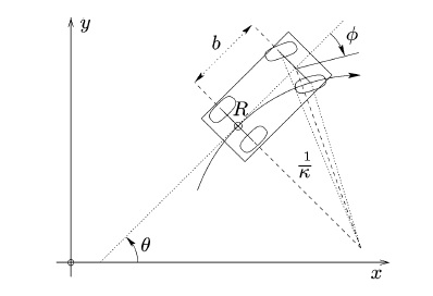
When low velocity (which implies the slipping rate goes to zero) is assumed, a kinematic model sufficiently characterizes the robot motion. By introducing an augmented configuration , We conduct path planning based on the following kinematic model [31]:
| (1) |
where is the curvature of the trajectory traversed by the robot, the velocity of the midpoint of the rear-wheel axle along the heading, and the steering rate. Let denote the wheelbase of the robot, then , and are related as follows:
The kinematic model (1) is subject to physical constraints on steering angle
| (2) |
and on control input
| (3) |
This implies that the curvature satisfies
| (4) |
Given constraints (2) - (4), the set of admissible control inputs to model (1) is given by
| (5) |
where is the terminal planning time, is the set of all measurable functions defined over , and the admissible control domain .
While planning with respect to , we ignore the minimum-dimension requirement and call the configuration for brevity of notation. Thus, the configuration space is . A configuration is collision-free if the robot at does not overlap with obstacles in the environment. The set of all collision-free configurations is denoted . The path planning problem is formulated below.
II-C The Motion Control Problem
The robot needs to follow as accurately as possible through an underlying control system. Because of the mismatches between the model (1) and the true dynamics and errors in sensing modules, the robot’s true trajectory will deviate from , i.e., the trajectory tracking error . When exceeds some obstacle clearance threshold , could fail to be collision-free. Hence, the top priority of the control system is to ensure that .
In view of the trade-off between the fidelity of the dynamics model (dynamic feasibility) and complexity of control design, we consider a dynamics model by augmenting the kinematics model (1) with two additional states . The state of the dynamic model reads:
| (6) |
where represents the actual front steering angle. Approximating the dynamics from the steering command to the actual front steering angle as a first-order system with time constant , we can express the dynamics model as follows:
| (7) |
The model 7 contains two control inputs,
| (8) |
Now We can define the motion control design problem.
Problem 2 (Motion Control)
Consider the dynamics model (7). Given a reference trajectory , an initial state with its image on being as the initial configuration, design a controller to command the robot such that whenever the robot’s actual initial configuration satisfies , its trajectory will satisfy , where are the thresholds for configuration and trajectory tracking errors, respectively.
III Path Planning via Continuous-curvature Steering
This section solves the path planning problem by first presenting the CC-BiRRT planner, then establishing the existence conditions of representative sub-optimal CC paths, which describe the pattern of reference trajectories to be generated, and finally conducting preliminary analysis.
Notation: A node is referred to as a collision-free configuration . An edge represents a feasible (collision-free and kinematically admissible) path between the two nodes. A tree is denoted by , where and are the node set and the edge set, respectively. For a set , denotes the number of elements. Start tree and goal tree are rooted at and , respectively. Given , an neighboring ball of is defined as , where is a distance function, e.g. , a weighted -norm: where is a positive semi-definite weighting matrix.
III-A CC-BiRRT: RRT-based Path Planning
Problem 1 is solved by adopting BiRRT, detailed as Algorithms 1-3. It constructs tree , where two kinematic RRT trees and grow toward each other until connected. Two trees are connected if there exists an edge with , and vice versa.
: returns according to a uniform sampling scheme. : grows tree toward . : returns that is closest to , and stays inside the -neighborhood: . That is:
The configuration is appended to only if there exists a collision-free path (edge) between and . : determines if an edge exists between and . : returns a set containing possibly various admissible paths each of which connects and . : checks whether is collision-free.
In Algorithm 1, both trees are connected if is true, equivalent, the configuration can be connected to and . Here is named after common node. The algorithm could return once such a common node is found. Alternatively, Algorithm 1 can run in anytime fashion: it keeps running and adding common nodes until reaches .
Key components of the aforementioned planner are the sampling, steering, and collision check, all of which are influential to the computation efficiency. Steering, taking care of the system kinematics or dynamics and thus being crucial to the positioning accuracy, is of our primary interest.
III-B CC Steering
The steering aims at finding a feasible and shortest path that can connect two configurations while avoiding collision with obstacles. Now we assume that a CC steering trajectory can be represented by a series of consecutive configurations, Problem 1 can be rephrased as the following CC steering problem.
Problem 3 (CC Steering)
Given as the initial and final configurations, respectively, determine a trajectory with such that it satisfies (1) with and .
Remark 1
If in addition the trajectory is required to give the shortest path length, Problem 3 is the shortest CC steering problem, which can be solved by assuming a normalized velocity, i.e., . When , the shortest CC steering problem reduces to RS steering [11]; and its solution always exists and comprises straight line segments and circular arcs of the minimum turning radius . Notably, previous work [11] has established that the RS steering solution admits one of 12 classes of structures: , where , , and represent the circular arc, the line segment, and the cusp, respectively. Since each represents four patterns: left forward , left backward , right forward , and right backward , RS paths admit 48 driving patterns.
As in [1], we assume that have null-curvature configurations, i.e., ; and solve for a special class of CC paths which combine a finite number of arcs: clothoid arcs, circular arcs, and straight line segments according to a certain structure in . Following the idea in [1], we derive explicit conditions for such a special class of CC paths to exist. The derivation is based on concepts: clothoid turns (CTs), clothoid circles (CCs), and -tangency conditions, which are introduced in Appendix for brevity of presentation. Existence conditions of two examples of CC path structures, namely and , are presented below through geometric analysis, respectively, whereas the derivation for the rest classes can be found in [41].
We introduce the following concept to simplify computation and reduce the number of cusps in CC paths.
Definition 1 (Valid Paths)
A CC path is valid if
-
(i)
any CT admits either a positive deflection or a negative deflection ; and
-
(ii)
there is no cusp in any CT.
Remark 2
CC steering with valid paths does not satisfy small-time controllability property [1]. As a result, integrating the CC steering with RRT does not offer completeness guarantee. This however does not pose a critical concern in practice. Actually, small-time controllability is a sufficient (but not necessary) condition to ensure that the true trajectory stays inside a small neighborhood of the trajectory reference. The same outcome can be guaranteed by either a complete steering and a mediocre tracking controller, or an incomplete (but kinematically feasible) steering and a high-performing tracking controller. We adopt the latter scheme, which nicely balances the demand on planner and controller.
III-B1
Taking as an example, we determine three intermediate configurations , , , as shown in Fig.3.
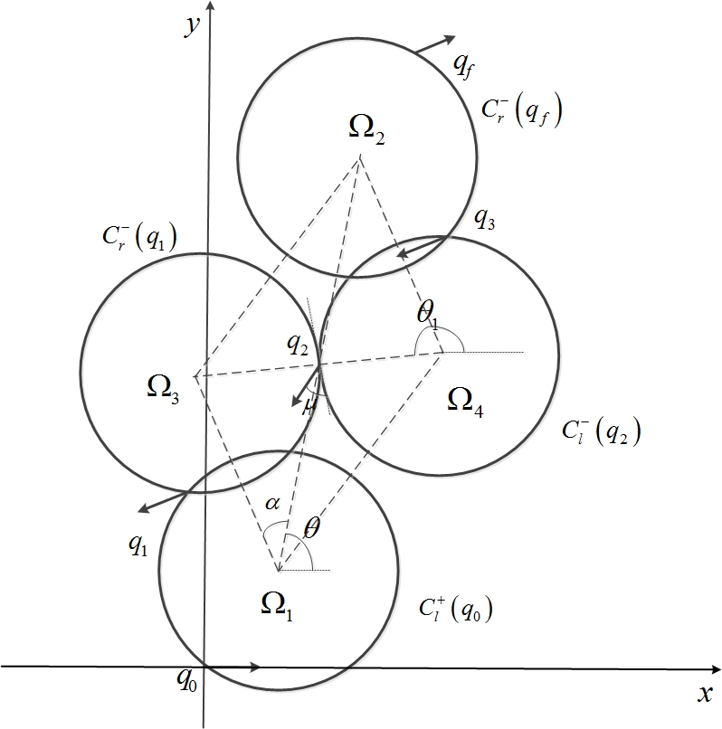
Let and be the centers of CC Circles and associated with and , respectively; and be the angle between the line and the positive -axis. As shown in Fig. 3, and is the center of and , respectively. The -tangency condition of and , and of and implies that
| (9) |
where is abused as an operator to calculate the length of a line. The -tangency between and implies We further have the following result.
Proposition 1
The lines and are in parallel.
Proof:
Let be the angle between and the positive -axis, and be the angle between and the positive -axis. The -tangency of and implies the orientation of is . Thus, after a backward right CT with deflection , the orientation of is and similarly, the orientation of is .
Meanwhile, serving as the initial configuration of the final backward right CT connecting and , the -tangency of and assures the orientation of to be . Thus , i.e., lines and are in parallel. ∎
It follows immediately from (9) and Proposition 1 that forms a parallelogram. Let denote the angle between and . Applying the law of cosines within the triangle yields
| (10) |
The coordinates of and can be expressed as functions of and :
| (11) |
The CC path is the concatenation of
-
(i)
a left forward CT1 with deflection ;
-
(ii)
a right backward CT2 with deflection ;
-
(iii)
a left backward CT3 with deflection .
-
(iv)
a right forward CT4 with deflection .
Existence Conditions (i) , and satisfy Definition 1; (ii) is a valid triangle, i.e.,
| (12) |
III-B2
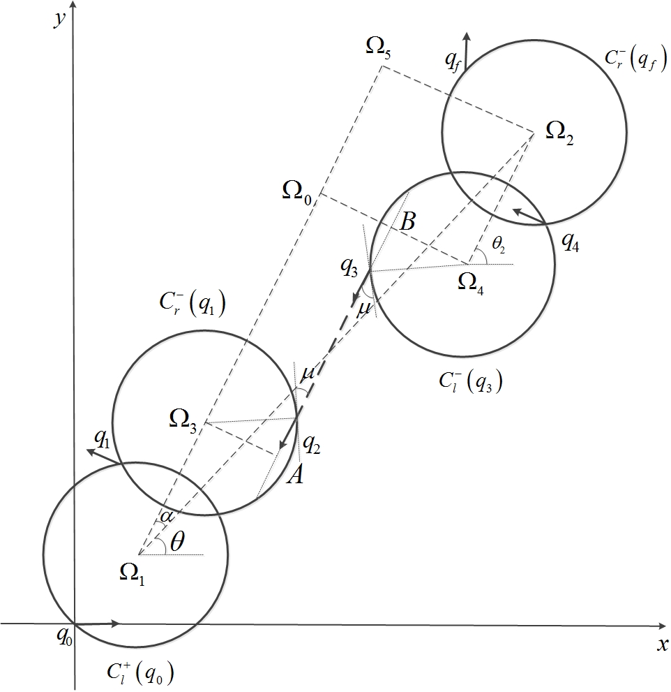
Similar to class, we derive the conditions that ensures the existence of a valid path. The setup for geometric analysis is depicted in Fig. 4 where denotes the angle between and the positive -axis. To appropriately determine intermediate configurations , , and , we introduce the following result.
Proposition 2
The lines and are in parallel.
Proof:
Let and be the angles between , and the positive -axis, respectively. The -tangency between and enforces the heading of to be , and the deflection of the right backward CT suggests that the orientation of and be . Therefore, after the left backward CT with deflection , the orientation of shall be . Also, the -tangency between and implies that the orientation of is . Thus , i.e., is parallel to . The proof is completed. ∎
Let be perpendicular to . Since forms an path from to , one can tell that . Furthermore, let be the point on line such that is perpendicular to . From Proposition 2, and is parallel to , making a square. Finally, the angle can be determined from the right triangle as follows:
| (13) |
One concludes from (13) that the path can be formed by composing
-
(i)
a left forward CT1 with deflection ;
-
(ii)
a right backward CT2 with deflection ;
-
(iii)
a backward line segment of length
-
(iv)
a left backward CT3 with deflection ;
-
(v)
a right forward CT4 with deflection .
Existence Conditions (i) and satisfy Definition 1; (ii) , which is equivalent to
| (14) |
III-C Motion Planning
Solving Problem 1 ends up with a CC path consisting of a sequence of CC steering solutions, i.e., the path comprises CTs and lines where each CT contains up to two clothoids and one circle. A clothoid arc is characterized by a non-zero steering rate , moving direction , and arc length , whereas both the circular arc and the line arc are characterized by a zero steering rate , moving direction , and arc length . Hence, any arc of a CC path is uniquely determined by its initial configuration and action . Since RS arcs are either circular or straight, both RS and CC arcs can be fully characterized by the following information - motion primitive (MP):
Thus an RS or a CC path, consisting of arcs, are formed by a sequence of MPs: .
The generation of reference trajectory, , based on MPs essentially determines the profiles of the longitudinal velocity and steering rate. The longitudinal velocity profile is determined by first counting the number of cusps in ; and for repeating the following two steps: 1) get the th group of consecutive MPs which have the same direction of movement and record the indices (here and ); 2) plan a trapezoidal velocity profile over for the th group with , and the path length being . Then one can obtain the velocity profile by concatenating all , and the steering rate profile according to the formulae
which is equivalent to
One can obtain the reference trajectory by integrating the model (1), where control input is specified by .
III-D Analysis
The existence conditions and the resultant CC steering algorithm are validated through simulation. We examine the feasibility and computation time of constructing RS and CC paths connecting to 1000 different ’s, where is randomly drawn from the domain . The CC steering algorithm finds feasible CC paths for all cases. However, as shown in Table I, for a steering problem, the average number of feasible CC paths is 8.6280, much less than that of feasible RS paths, which is 24.32. Feasibility time in Table I is the time taken to check feasibility by verifying existence conditions of all 48 driving patterns, whereas path time quantifies the time taken to compute the shortest path according to the outcome of the feasibility check. The feasibility check of CC steering is 19 times slower than RS case, and it takes 22 times longer to construct a CC path than for the RS path case.
| RS | CC | Ratio | |
|---|---|---|---|
| Feasible Paths (Avg.) | 24.3200 | 8.6280 | 2.8187 |
| Feasibility Time (Avg.) | 0.5579 ms | 10.4220 ms | 18.6722 |
| Path Time (Avg.) | 0.1260 ms | 2.8193 ms | 22.3278 |
Table I shows that CC path generation requires much lighter computation (2.82 ms) than verifying the feasibility (10.42 ms); thus, one wonders whether the feasibility results of RS steering can be exploited to improve the computation efficiency of CC steering. We have the following result.
Proposition 3
Given two configurations, the existence of a valid CC path in the class of implies the existences of an RS path in the same class.
Proof:
A sketch of the proof is provided below. We use as an example to show that if there exists a CC path of a given pattern, then an RS path with the same pattern also exists. The existence of the -type CC path between and implies conditions (14). From Fig. 13, we know . From Fig. 4, we have , where represent the centers of minimum turning circles passing , , respectively. Similarly, based on the CC condition , one can establish
We verify all existence conditions of -type RS path, which imply the existence of such RS path. ∎
Proposition 3 states that for a CC path exists, the existence of an RS path with the same pattern is necessary. This allows us to reduce computation time of CC steering by only testing feasible classes of RS steering problem. Simulation shows this treatment saves computation time than running feasibility check for all 12 classes.
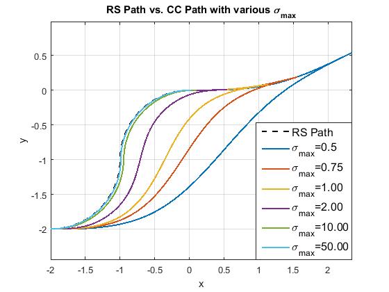
Next, we elaborate that as increases, the sequence of CC paths converges to the RS path. This is illustrated by solving for an path from to with varying from to . As shown in Fig. 5, the sequence of CC paths converges to the RS path.
IV NMPC Trajectory Tracking Control
To illustrate the benefits of employing a CC path rather than an RS path in trajectory tracking, we deploy the two kinds of paths in an autonomous parking scenario. A planner, based on either the CC steering or the RS steering, first generates the desired CC or RS trajectories. Then, an NMPC endeavors to accurately follow the references. Note that for both the RS and the CC cases, the configuration and the parameter tuning of the NMPC remain exactly the same.
IV-A Nonlinear Model Predictive Control Formulation
The NMPC generates the optimal speed and steering commands to track the reference trajectories , , , while respecting the actuator and safety constraints. Based on (6) and (8), we formulate the cost function to minimize as:
| (15) | ||||
In (15), represents the prediction horizon. , , , and are the weighting factors. The reference virtual inputs , and the reference states, generated from either a CC planner or an RS planner, are . corresponds to the non-negative slack variables. The first term leads the predicted vehicle states within the prediction horizon to converge towards their reference values. The second term penalizes the commands interventions. The last two terms are the soft constraints violations penalties.
Grounded on the cost function (15), we express the constrained optimization problem as:
| (16) | ||||
Eq. represents the periodical state feedback. Eq. indicates the discretized vehicle model in (7). Eqs. , , and summarize the soft constraints on the actual front steering angle , the steering angle command , and the speed command . The equations , condense the hard constraints on the virtual system inputs, defined in (8). With the help of the non-negative slack variables, we soften the constraints in , , and to ensure recursive feasibility. Sufficiently large weights and in the cost function (15) guarantee that whenever the constraints can be satisfied.
Solving the constrained optimization problem (16) yields the optimal input sequence within the prediction horizon: . The optimal high-level commands from NMPC at the current step , read:
| (17) |
where , correspond to the optimal acceleration and steering rate (see eq. (8)), and is the sampling period of the NMPC. The NMPC implementation details can be found in [42].
During simulation, the steering command was directly sent to the CarSim vehicle model for front steering control. In contrast, a low-level speed controller [43] was included to regulate the four wheels’ torques of the CarSim model, such that the speed command from the NMPC could be achieved.
V Case Study: Sampling-based Planning & Control for Autonomous Parking
The showcased autonomous parking maneuver requires a passenger car fixed at to stabilize around the terminal condition , which corresponds to a typical perpendicular parking maneuver. BiRRT along with either the RS steering or the CC steering is employed to generate a reference trajectory. An NMPC is then leveraged for accurately following the references. We first compare the execution time to generate the two types of paths, and then employ CarSim-Simulink joint simulations to demonstrate the benefits of adopting CC paths in improving the trajectory following performance of the NMPC formulated in Section IV-A.
V-A Execution Time for Reference Generation
We run Monte Carlo simulation to mitigate the effect of randomness in RRT sampling. The evaluation is based on the platform: 4GHz quad-core i7 and Matlab 2020b. We run 1000 simulations of each algorithm and RS steering results in a mean time 0.23 sec and average number of cusps 4.50; the CC steering results in a mean time 2.29 sec with average number of cusps being 4.46 (the steering rate is rad/sec). The computation of CC steering is significantly heavier at 9 times slower than RS steering, whereas the numbers of cusps of the resultant paths are similar for both cases. When the steering rate is slower, saying rad/sec, the mean computation time for CC steering-based planning further reaches 4.36 sec, and the mean number of cusps goes up to 6.26.
V-B CarSim-Simulink Joint Simulation
Although the CC-RRT requires a relatively longer execution time to find a feasible path, as we will see, the smoother trajectories issued from the CC-RRT can facilitate the trajectory tracking of the NMPC. CarSim-Simulink joint simulation is executed for validation. In CarSim, the simulated plant falls into the category of a C-Class Hatchback, with a wheelbase . Pacejka 5.2 tire model is employed to simulate the tire forces. The mismatch between the simplified vehicle dynamic model (7) and the high-fidelity CarSim model contributes to trajectory tracking errors.
The major parameters inside the NMPC controller are tuned as: , , , , . The control constraints include: , , , and .
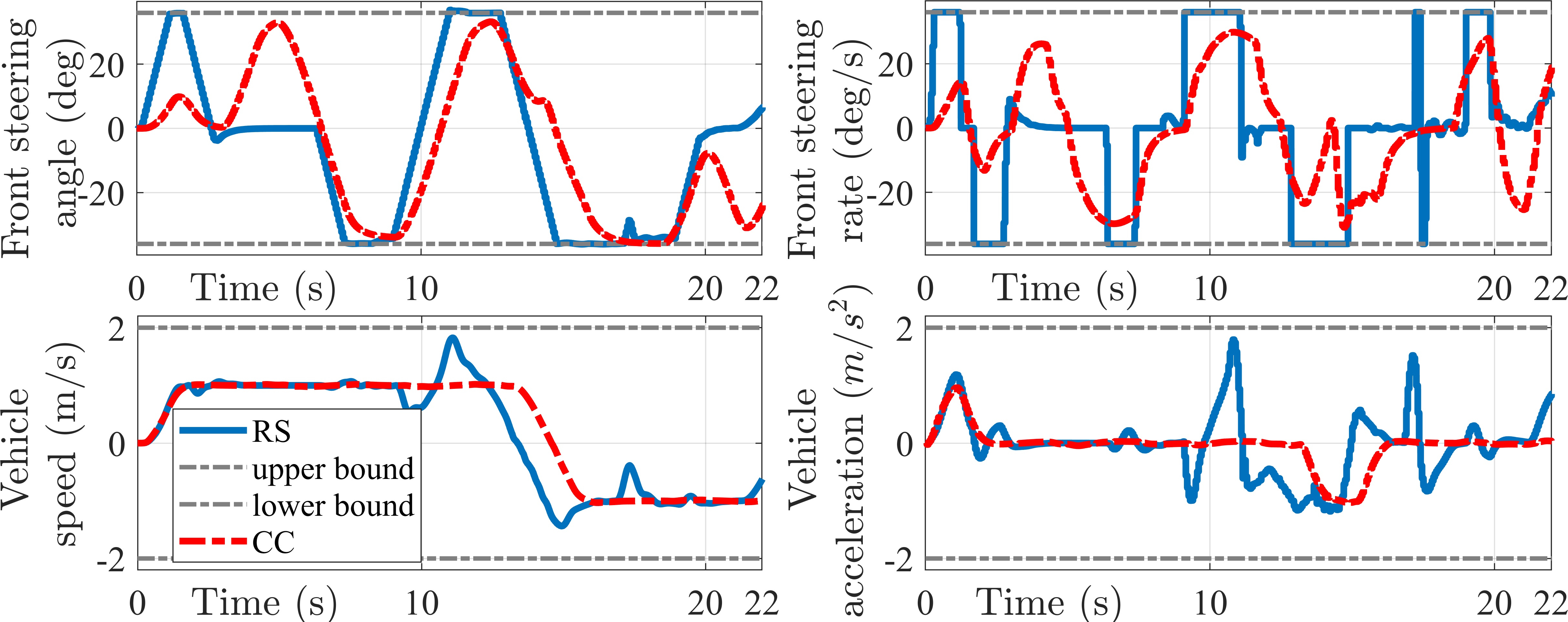
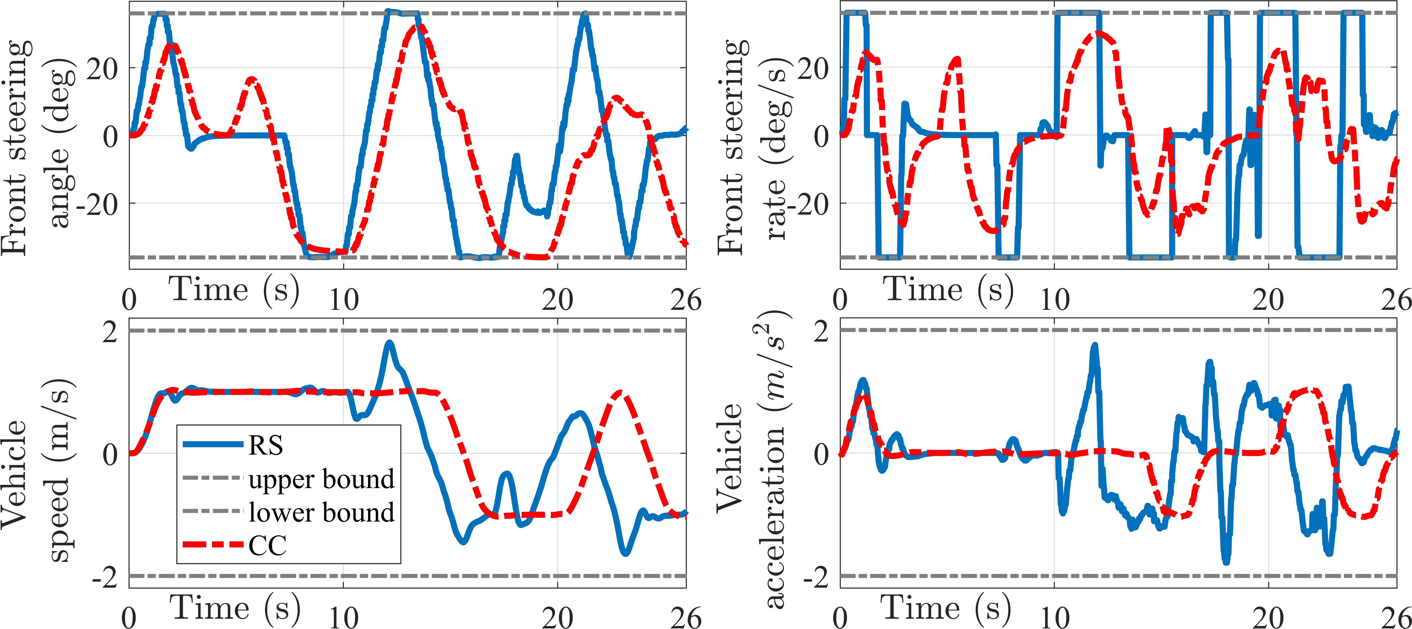
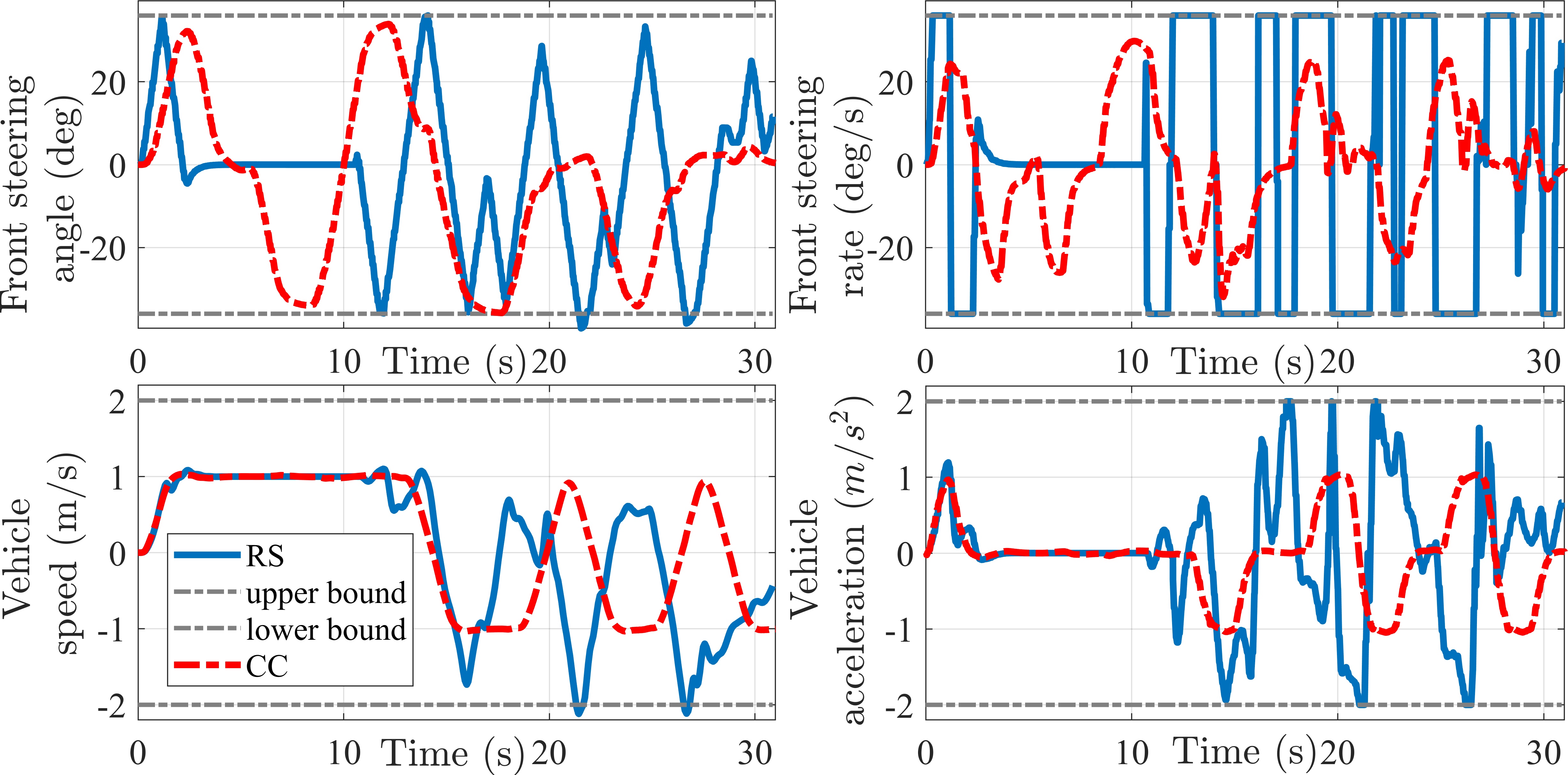
We first show the representative control and trajectory following results when there exist, respectively, one, three, or five cusps in the generated reference paths. Figs.6-7 demonstrate the trajectory following results and the commands of the NMPC following an RS path and a CC path with one cusp. Similarly, the results when there exist three and five cusps in the generated paths are depicted in Figs.8-11.
![]()
![]()
![]()
As manifested in Fig.6, Fig.8, and Fig.10, the trajectory tracking performance of the exactly same NMPC substantially improves if the generated reference path (RS Path∗, CC Path∗) comes from CC-RRT. For instance, the maximum absolute value of the lateral offset:
| (18) |
in Fig.6 reduce from over 0.4m to less than 0.1m if the generated path is issued from CC-RRT instead of the RS-RRT. In addition, the speed tracking error also decreases if the CC-RRT path is used. Since the inter-vehicle distance is quite limited in the studied parking scenario, employing a CC trajectory could substantially reduce the collision possibility.
The underlying reason that the CC-RRT path enhances the trajectory tracking performance of the NMPC is revealed in Fig.7, Fig.9, and Fig.11: The RS-RRT path, which contains path curvature derivatives with infinite magnitudes, enforces the front steering rate of NMPC approaching its hard constraint . Since the actual steering rate can never reach the desired value , the steering angle further moves towards its limit for compensation. With both and constrained at their limit, the path tracking performance, as reflected in the lateral offset and the yaw error , continues to deteriorate, which finally requires the NMPC to sacrifice the less-weighted speed tracking error to minimize the cost function in (15).
On the contrary, the CC-RRT path, which explicitly considers the change rate of the curvature, is able to yield a path with the required steering rate well below the vehicle actuator limit. As demonstrated in Fig.7, Fig.9, and Fig.11, when following the path generated from CC-RRT, both the steering angle and the steering rate of the NMPC fall below their corresponding thresholds and the actuator constraints are rarely touched. Such an effortless steering control improves the path tracking performance. Consequently, the NMPC can pay more attention to the speed tracking error to render the cost function minimum.
To statistically verify if employing the CC-RRT paths can improve the control performance of the NMPC, we execute multi-simulations. We first generate three groups of paths, with each group containing two hundred paths with respectively, one, three, and five cusps. Within each group, half of the paths are generated from RS-RRT, and the rest are generated from CC-RRT. We calculate the root-mean-square (RMS) of the trajectory tracking errors, including the lateral offset , the speed tracking error , and the yaw error . The box plots of the tracking errors are summarized in Fig. 12.
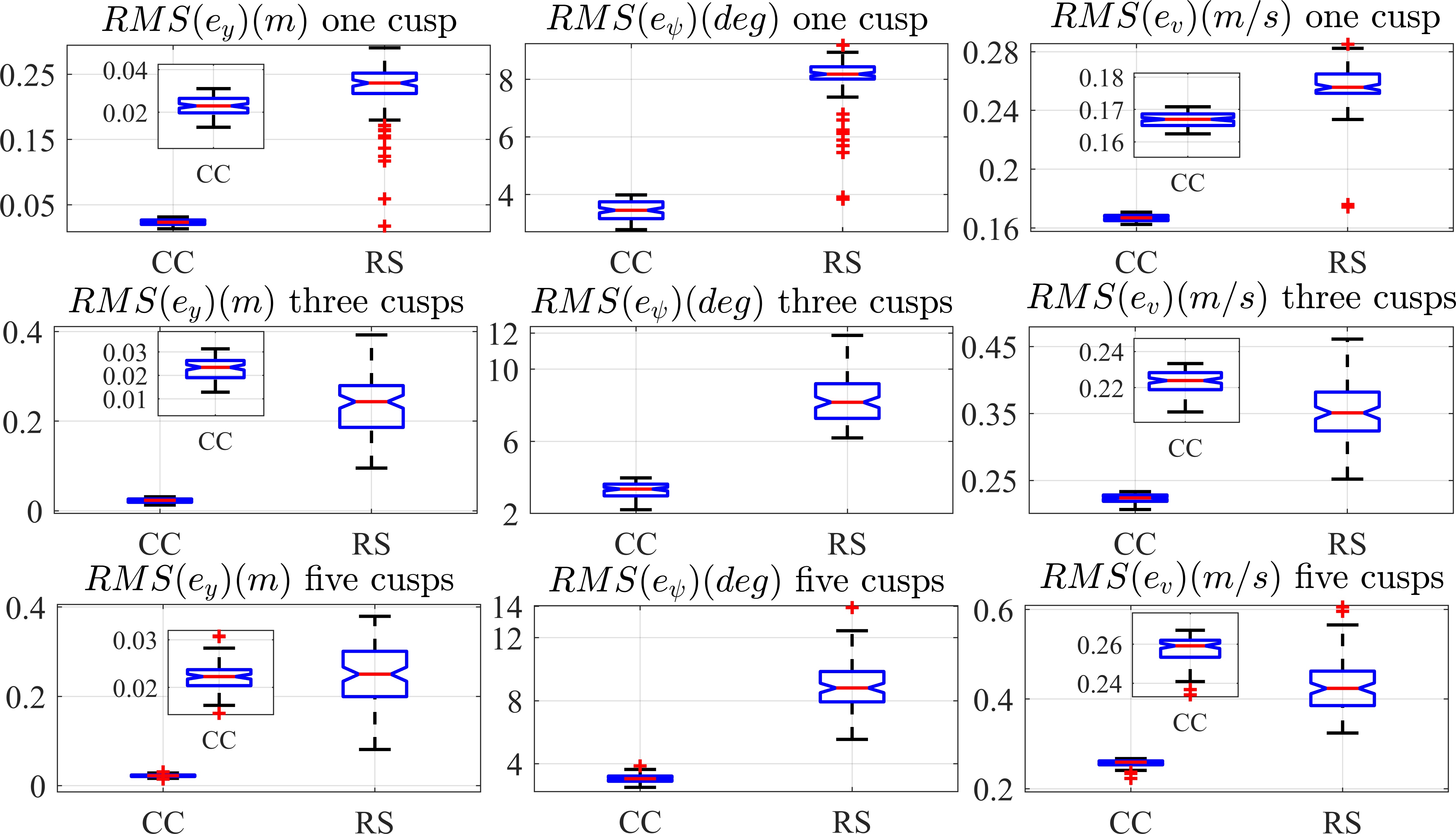
As shown in Fig.12, no two box notches in any of the nine box plots overlaps. Therefore, we can conclude, with confidence, that the NMPC can more accurately follow the path generated from the CC-RRT than the RS-RRT.
VI Conclusion
Path planning and motion control design have been studied in this paper for mobile robots with car-like dynamics. On the one hand, path planning problem is solved by incorporating RRT-based planning algorithms with continuous-curvature steering techniques, and geometric analysis is carried out to guarantee existence of certain continuous-curvature sub-optimal paths that are composed of straight line segments and clothoid turns that satisfy constraints on velocity, curvature and derivative of the curvature. On the other hand, nonlinear MPC approaches are utilized to generate speed and steering commands to guide the robot to track the generated reference trajectories in an optimized manner. CarSim-Simulink joint simulation reveals that the continuous-curvature path is easier to follow for a standard nonlinear model predictive controller. Future research directions may include study of path planning for multi-robot case and motion control in the presence of more types of model and/or environment uncertainties.
[Proof of the Zonklar Equations]
The concepts of clothoid turns (CT) and -tangency are introduced for completeness. Readers are referred to [11, 1, 41] for details.
-A Clothoid Turn
A clothoid is a curve whose curvature is an affine function of its arc length , i.e., , with denotes the sharpness of the clothoid. A clothoid starting at a configuration is given by
| (19) |
where is the arc length from , and
| (20) |
are the Fresnel cosine and sine integrals, respectively.
Given and , the difference in headings is defined as deflection: . For a clothoid with and ending at , it induces a deflection .
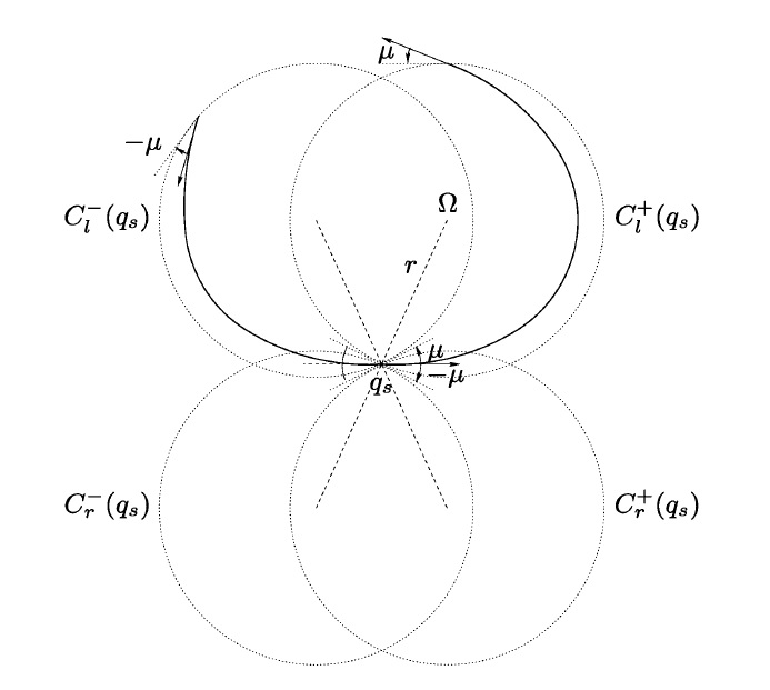
A CT from to consists of three components: two clothoids and a circular arc. The radius of the circular arc is not necessarily the minimum turning radius . There are four types of CTs: left forward, left backward, right forward, and right backward. Below illustrates how to use a left forward CT to achieve a deflection .
Case 1: . Robot follows a first clothoid with sharpness until the curvature reaches . According to (19), the first clothoid ends at the intermediate configuration with . From , the robot enters a circular arc of radius and of an angular value . The center of the circle has the coordinates given by The circular arc ends at a second intermediate configuration . Finally the robot follows a second clothoid with sharpness until it reaches .
Remark 3
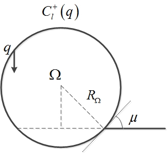
The locus of the starting and the goal configurations forms a circle centered at . The circle is named as left forward CC Circle and is denoted as . All four CC circles corresponding to four types of CTs are depicted in Fig. 13. The radius of the CC Circle and the angle between the orientation of and the tangent of at are obtained as follows, respectively:
| (21) |
Case 3: . The circular arc is absent from the CT, and hence the CT is composed of
-
(i)
a clothoid of sharpness starting from ;
-
(ii)
a symmetric clothoid of sharpness ending at .
For computational efficiency, we require that . Toward this end, the sharpness is computed as
| (22) |
and the arc length of each clothoid is .
Case 3: . The CT reduces to a straight line from to . The arc length is to ensure that .
Remark 4
Left forward CT can achieve a positive deflection of . However, it gives an invalid path according to Def. 1 because the deflection exceeds or it contains cusps. In order to achieve the same change of heading, the valid path should have a negative deflection by considering the fact that a positive deflection is equivalent to a negative deflection . In particular, to achieve , the robot moves backward by following a left backward CT:
-
(i)
a clothoid from to with sharpness and length ;
-
(ii)
a circular arc of radius and of angle , from to ;
-
(iii)
a clothoid from to with sharpness and length .
It can be verified that both and are located on .
-B -Tangency
The -tangency condition is analogous to its counterpart in forming RS paths [11]. There are two cases: the first stipulates how a line segment should be concatenated to a CT; the second specifies how two CTs should be connected. For the first case, the line segment must cross the corresponding CC circle at an angle of . Fig. 14 illustrates the -tangency condition for an motion starting from a configuration .
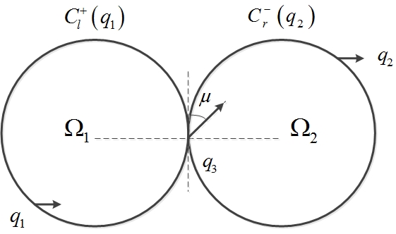
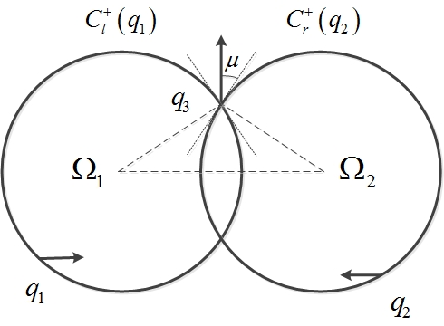
The -tangency condition between two consecutive CTs depends on whether the robot’s motion contains cusps or not. For no cusp case, take an motion from to as an example. As shown in Fig. 15, the -tangency condition suggests that the CC circle be tangent to at ; and the angle between the orientation of and tangent vectors of both is . For cusp case, the -tangency condition for an motion from to is illustrated in Fig. 16. Let be the cusp configuration, and must be located at one of the two intersecting points of the CC Circles and . The -tangency condition is that the orientation of forms an angle of with respect to the tangent vectors of both CC Circles, or equivalently the orientation of the robot at is vertical to the line .
References
- [1] T. Fraichard and A. Scheuer, “From Reeds and Shepp’s to continuous-curvature paths,” IEEE Trans. Robot., vol. 20, no. 6, pp. 1025–1035, 2004.
- [2] J.-P. Laumond, P. E. Jacobs, M. Taix, and R. M. Murray, “A motion planner for nonholonomic mobile robots,” IEEE Trans. Robot. Automat., vol. 10, no. 5, pp. 577–593, 1994.
- [3] Y. J. Kanayama and B. I. Hartman, “Smooth local-path planning for autonomous vehicles,” Int. J. Robot. Res., vol. 16, no. 3, pp. 263–284, 1997.
- [4] K. M. Choset, H. M. Lynch, S. Hutchinson, G. Kantor, W. Burgard, L. E. Kavraki, and S. Thrun, Principles of Robot Motion: Theory, Algorithms, and Implementation. Boston: MIT Press, 2005.
- [5] S. M. LaValle, Planning Algorithms. Cambridge, U.K.: Cambridge University Press, 2006.
- [6] C. Belta, A. Bicchi, M. Egerstedt, E. Frazzoli, E. Klavins, and G. J. Pappas, “Symbolic planning and control of robot motion [Grand challenges of robotics],” IEEE Robot. Autom. Mag., vol. 14, no. 1, pp. 61–70, 2007.
- [7] G. E. Fainekos, A. Girard, H. Kress-Gazit, and G. J. Pappas, “Temporal logic motion planning for dynamic robots,” Automatica, vol. 45, no. 2, pp. 343–352, 2009.
- [8] K. P. Valavanis and G. N. Saridis, Intelligent Robotic Systems: Theory, Design and Applications. Berlin: Springer, 2012, vol. 182.
- [9] J. Fu, F. Tian, T. Chai, Y. Jing, Z. Li, and C.-Y. Su, “Motion tracking control design for a class of nonholonomic mobile robot systems,” vol. 50, no. 6, pp. 2150–2156, 2020.
- [10] L. E. Dubins, “On curves of minimal length with a constraint on average curvature, and with prescribed initial and terminal positions and tangents,” Amer. J. Math., vol. 79, no. 3, pp. 497–516, 1957.
- [11] J. Reeds and L. Shepp, “Optimal paths for a car that goes both forwards and backwards,” Pac. J. Math., vol. 145, no. 2, pp. 367–393, 1990.
- [12] P. R. Giordano, M. Vendittelli, J.-P. Laumond, and P. Soueres, “Nonholonomic distance to polygonal obstacles for a car-like robot of polygonal shape,” IEEE Trans. Robot., vol. 22, no. 5, pp. 1040–1047, 2006.
- [13] D. V. Dimarogonas and K. J. Kyriakopoulos, “On the rendezvous problem for multiple nonholonomic agents,” IEEE Trans. Autom. Control, vol. 52, no. 5, pp. 916–922, 2007.
- [14] E. Plaku and S. Karaman, “Motion planning with temporal-logic specifications: Progress and challenges,” AI Communications, vol. 29, no. 1, pp. 151–162, 2016.
- [15] D. González, J. Pérez, V. Milanés, and F. Nashashibi, “A review of motion planning techniques for automated vehicles.” IEEE Trans. Intell. Transp. Syst., vol. 17, no. 4, pp. 1135–1145, 2016.
- [16] S. Xu, R. Zidek, Z. Cao, P. Lu, X. Wang, B. Li, and H. Peng, “System and experiments of model-driven motion planning and control for autonomous vehicles,” vol. 52, no. 9, pp. 5975–5988, 2022.
- [17] I. Maurović, M. Seder, K. Lenac, and I. Petrović, “Path planning for active SLAM based on the D* algorithm with negative edge weights,” vol. 48, no. 8, pp. 1321–1331, 2017.
- [18] H. Vorobieva, S. Glaser, N. Minoiu-Enache, and S. Mammar, “Automatic parallel parking in tiny spots: path planning and control,” IEEE Trans. Intell. Transp. Syst., vol. 16, no. 1, pp. 396–410, 2015.
- [19] R. Quirynen, K. Berntorp, K. Kambam, and S. Di Cairano, “Integrated obstacle detection and avoidance in motion planning and predictive control of autonomous vehicles,” in 2020 American Control Conference (ACC). IEEE, 2020, pp. 1203–1208.
- [20] P. Falcone, F. Borrelli, J. Asgari, H. E. Tseng, and D. Hrovat, “Predictive active steering control for autonomous vehicle systems,” IEEE Transactions on Control Systems Technology, vol. 15, no. 3, pp. 566–580, 2007.
- [21] Z. Li, J. Deng, R. Lu, Y. Xu, J. Bai, and C.-Y. Su, “Trajectory-tracking control of mobile robot systems incorporating neural-dynamic optimized model predictive approach,” vol. 46, no. 6, pp. 740–749, 2016.
- [22] I. Matraji, A. Al-Durra, A. Haryono, K. Al-Wahedi, and M. Abou-Khousa, “Trajectory tracking control of skid-steered mobile robot based on adaptive second order sliding mode control,” Control Engineering Practice, vol. 72, pp. 167–176, 2018.
- [23] W. Shi, S. Song, C. Wu, and C. P. Chen, “Multi pseudo q-learning-based deterministic policy gradient for tracking control of autonomous underwater vehicles,” IEEE Transactions on Neural Networks and Learning Systems, vol. 30, no. 12, pp. 3534–3546, 2018.
- [24] A. Alouache and Q. Wu, “Fuzzy logic pd controller for trajectory tracking of an autonomous differential drive mobile robot (ie quanser qbot),” Industrial Robot: An International Journal, 2018.
- [25] L. Menhour, B. d’Andréa Novel, M. Fliess, D. Gruyer, and H. Mounier, “An efficient model-free setting for longitudinal and lateral vehicle control: Validation through the interconnected pro-sivic/rtmaps prototyping platform,” IEEE Transactions on Intelligent Transportation Systems, vol. 19, no. 2, pp. 461–475, 2017.
- [26] A. Eskandarian, C. Wu, and C. Sun, “Research advances and challenges of autonomous and connected ground vehicles,” IEEE Transactions on Intelligent Transportation Systems, 2019.
- [27] S. Karaman and E. Frazzoli, “Sampling-based algorithms for optimal motion planning,” Int. J. Robot. Res., vol. 30, no. 7, pp. 846–894, 2011.
- [28] L. E. Kavraki, P. Svestka, J.-C. Latombe, and M. H. Overmars, “Probabilistic roadmaps for path planning in high-dimensional configuration spaces,” IEEE Trans. Robot. Automat., vol. 12, no. 4, pp. 566–580, 1996.
- [29] S. M. LaValle and J. J. Kuffner Jr., “Randomized kinodynamic planning,” Int. J. Robot. Res., vol. 20, no. 5, pp. 378–400, 2001.
- [30] M. Elbanhawi and M. Simic, “Sampling-based robot motion planning: A review,” IEEE Access, vol. 2, pp. 56–77, 2014.
- [31] J.-D. Boissonnat, A. Cerezo, and J. Leblond, “A note on shortest paths in the plane subject to a constraint on the derivative of the curvature,” INRIA Research Report-2160, 1994.
- [32] H. J. Sussmann, “The Markov-Dubins problem with angular acceleration control,” in Proc. the 36th IEEE Conf. Decision and Control (CDC), vol. 3. IEEE, 1997, pp. 2639–2643.
- [33] J. Villagra, V. Milanés, J. Pérez, and J. Godoy, “Smooth path and speed planning for an automated public transport vehicle,” Robot. Auton. Syst., vol. 60, no. 2, pp. 252–265, 2012.
- [34] M. Brezak and I. Petrović, “Real-time approximation of clothoids with bounded error for path planning applications,” IEEE Trans. Robot., vol. 30, no. 2, pp. 507–515, 2014.
- [35] A. Scheuer and C. Laugier, “Planning sub-optimal and continuous-curvature paths for car-like robots,” in Proc. 1998 IEEE/RSJ Conf. Intell. Robot. Syst. (IROS), vol. 1. IEEE, 1998, pp. 25–31.
- [36] E. Bakolas and P. Tsiotras, “On the generation of nearly optimal, planar paths of bounded curvature and bounded curvature gradient,” in Proc. the 2009 Amer. Control Conf. (ACC). IEEE, 2009, pp. 385–390.
- [37] K. Yang and S. Sukkarieh, “An analytical continuous-curvature path-smoothing algorithm,” IEEE Trans. Robot., vol. 26, no. 3, pp. 561–568, 2010.
- [38] G. Klančar, M. Seder, S. Blažič, I. Škrjanc, and I. Petrović, “Drivable path planning using hybrid search algorithm based on E* and bernstein–bézier motion primitives,” vol. 51, no. 8, pp. 4868–4882, 2021.
- [39] T. Berglund, A. Brodnik, H. Jonsson, M. Staffanson, and I. Soderkvist, “Planning smooth and obstacle-avoiding B-spline paths for autonomous mining vehicles,” IEEE Trans. Autom. Sci. Eng., vol. 7, no. 1, pp. 167–172, 2010.
- [40] F. Ghilardelli, G. Lini, and A. Piazzi, “Path generation using -splines for a truck and trailer vehicle,” IEEE Trans. Autom. Sci. Eng., vol. 11, no. 1, pp. 187–203, 2014.
- [41] J. Dai and Y. Wang, “On existence conditions of a class of continuous curvature paths,” in Proc. the 36th Chinese Control Conference (CCC). IEEE, 2017, pp. 6773–6780.
- [42] Z. Wang, A. Ahmad, R. Quirynen, Y. Wang, A. Bhagat, E. Zeino, Y. Zushi, and S. Di Cairano, “Motion planning and model predictive control for automated tractor-trailer hitching maneuver,” in 2022 IEEE Conference on Control Technology and Applications (CCTA). IEEE, 2022, pp. 676–682.
- [43] Z. Wang and J. Wang, “Ultra-local model predictive control: A model-free approach and its application on automated vehicle trajectory tracking,” Control Engineering Practice, vol. 101, p. 104482, 2020.