Selective Focus: Investigating Semantics Sensitivity
in Post-training Quantization for Lane Detection

Abstract

Lane detection (LD) plays a crucial role in enhancing the L2+ capabilities of autonomous driving, capturing widespread attention. The Post-Processing Quantization (PTQ) could facilitate the practical application of LD models, enabling fast speeds and limited memories without labeled data. However, prior PTQ methods do not consider the complex LD outputs that contain physical semantics, such as offsets, locations, etc., and thus cannot be directly applied to LD models. In this paper, we pioneeringly investigate semantic sensitivity to post-processing for lane detection with a novel Lane Distortion Score. Moreover, we identify two main factors impacting the LD performance after quantization, namely intra-head sensitivity and inter-head sensitivity, where a small quantization error in specific semantics can cause significant lane distortion. Thus, we propose a Selective Focus framework deployed with Semantic Guided Focus and Sensitivity Aware Selection modules, to incorporate post-processing information into PTQ reconstruction. Based on the observed intra-head sensitivity, Semantic Guided Focus is introduced to prioritize foreground-related semantics using a practical proxy. For inter-head sensitivity, we present Sensitivity Aware Selection, efficiently recognizing influential prediction heads and refining the optimization objectives at runtime. Extensive experiments have been done on a wide variety of models including keypoint-, anchor-, curve-, and segmentation-based ones. Our method produces quantized models in minutes on a single GPU and can achieve 6.4% F1 Score improvement on the CULane dataset.

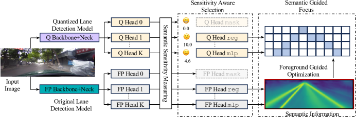
Figure 1: The framework of Selective Focus. Three modules are designed to mine the semantics sensitivity in the post-training quantized lane detection. Semantic Sensitivity Measuring measures the semantic sensitivity quantitatively; Sensitivity Aware Selection adapts the optimization objectives according to dynamic sensitivity. Semantic Guided Focus enables PTQ to focus on the foreground with a practical proxy.

1 Introduction

Deep neural networks have recently sparked great interest in autonomous driving. As a fundamental component in autonomous driving, lane detection (LD) is fundamental for high-level functions such as lane departure warning, lane departure prevention, etc. Lane detection (Qin, Wang, and Li 2020; Wang et al. 2022b; Tabelini et al. 2021) has garnered significant attention and undergone in-depth research, leading to substantial advancements. However, LD models are often required to run on edge devices within limited sizes, necessitating quantization and introducing formidable challenges to detection performance.

There are two prevalent quantization techniques: Quantization Aware Training (QAT) e.g. (Choi et al. 2018; Esser et al. 2019; Bhalgat et al. 2020; Jain et al. 2020) and Post- training Quantization (PTQ) e.g. (Hubara et al. 2020; Wu et al. 2020a; Wei et al. 2022; Wang et al. 2022a). Though QAT can often yield promising performance, it requires a longer training duration and the whole labeled dataset, raising computation costs and safety concerns. In contrast, PTQ methods have attracted wide attention from both industry and academia due to their speed and label-free nature. Recently, some PTQ methods (Nagel et al. 2020; Li et al. 2021; Wei et al. 2022) propose to tune the weight by reconstructing the original outputs, bringing better performance.

LD models typically regress semantic outputs with physical meanings such as offsets, locations, and angles, and employ complex post-processing to handle these outputs. Notably, the sensitivity of these semantic outputs to post-processing varies, with certain elements having the potential to induce significant lane deformation even with minor perturbations. Prior PTQ approaches employing direct reconstruction methods on feature maps treat all outputs uniformly, overlooking post-processing information.

In this paper, we first propose the semantic sensitivity in lane detection models and introduce a Lane Distortion Score to measure the quantization distortion between the original LD model and the corresponding quantized counterpart. Subsequently, we investigate these sensitivities from two perspectives, namely the intra-head sensitivity and the inter-head sensitivity. Specifically, the intra-head sensitivity highlights the heightened sensitivity of a limited number of foreground (lane) regions to quantization noise during post-processing, while the inter-head sensitivity indicates the varying degrees of sensitivity to the quantization of different semantic heads over time, as shown in Figure 4.

To address the sensitivity problems above, we propose a Selective Focus framework to alleviate the semantic sensitivity in post-training quantization for LD models, enhancing the performance. The proposed framework is deployed with a Semantic Guided Focus module and a Sensitivity Aware Selection module, respectively targeting the intra-head sensitivity and the inter-head sensitivity. First, the Semantic Guided Focus generates practical proxies of masks from semantics, enhancing the precision of foreground lanes in post-processing. This method guides PTQ to optimize these pivotal areas. Furthermore, the Sensitivity Aware Selection module refines optimization objectives by querying efficiently the real-time sensitivity of each head through our Lane Distortion Score across heads. The proposed framework could tune the models efficiently by introducing the semantic information of the post-process to the optimization implicitly.

To the best of our knowledge, our work is the first to identify the role of semantic sensitivity in PTQ for lane detection models, and we hope it could offer new insight to the community. Extensive experiments on the widely-used CULane dataset and various leading methods validate the effectiveness and efficiency of the proposed Selective Focus framework. In summary, our contributions are listed as follows:

• We introduce the concept of semantics sensitivity in post-processing quantization for lane detection, proposing the Lane Distortion Score metric. Our Selective Focus framework, composed of the Semantic Guided Focus and Sensitivity Aware Selection modules, addresses both intra-head and inter-head sensitivities.

• Considering the intra-head semantics sensitivity, the Semantic Guided Focus module generates practical proxy masks from semantics and thus guides PTQ to optimize these pivotal areas.

• Handling inter-head semantics sensitivity, the Sensitivity Aware Selection module efficiently adjusts optimization objectives based on each head’s real-time sensitivity measured by our Lane Distortion Score.

• Our empirical tests across datasets, models, and quantization setups endorse our approach’s efficacy. Notably, under the 4-bit setup, performance gains exceed up to 6.4%, on benchmark models with a 6x acceleration.

2 Related Works

2.1 Lane Detection Models

The LD task aims to produce lane representations in the given images. Despite the different methods, they all try to set the foreground (lanes) apart from the background. Nowadays the models generally use Convolutional Neural Networks (CNNs) to extract lane features, which can be divided into keypoint-based, anchor-based, segmentation-based, and parameterized-curve-based methods.

Keypoint-based Methods predict the mask of lane points and regress them to the real location on the corresponding lanes. CondLaneNet (Liu et al. 2021a) regresses offset between adjacent keypoints, while GANet (Wang et al. 2022b) regresses offset between each keypoint to the start point of its lane. Anchor-based Methods model lanes as pre-defined pairs of start point and angle, and then regress lanes among them. LaneATT (Tabelini et al. 2021) proposes an anchor attention module to aggregate global information for the regression. CLRNet (Zheng et al. 2022) refines the proposals with features at different scales. Segmentation-based Methods predict the mask of all the lanes on the image and then cluster them into different lanes. SCNN (Pan et al. 2018) adopts slice-by-slice convolution modules to aggregate surrounding spatial information. RESA (Zheng et al. 2021) further extends the mechanism to aggregate global spatial to every pixel. Curve-based Methods model lanes as singular curves, rather than sets of discrete points. For instance, LSTR (Liu et al. 2021b) predicts the parameters for cubic curves and BézierLaneNet (Feng et al. 2022) predicts for Bézier curves.

2.2 Post-traning Quantization

Quantization is widely used in deep learning model deployment to substantially cut down memory and computation requirements during inference, which is required by the LD models. Compared to QAT (Jacob et al. 2018; Gong et al. 2019; Jain et al. 2020; Esser et al. 2019; Bhalgat et al. 2020) which requires large GPU effort and the whole dataset, PTQ methods have sparked great popularity these days due to their speed and label-free property.

Common PTQ methods like OMSE (Choukroun et al. 2019) and ACIQ (Banner, Nahshan, and Soudry 2019) often identify quantization parameters to minimize the quantized error for tensors, requiring a few batches of forward passes. More recently, some methods have evolved to slightly tune the weights and reconstruct the original outputs. (Wu et al. 2020b) improves the accuracy by setting a well-defined target for the face recognition task. AdaRound (Nagel et al. 2020) initially proposes that adjusting the weight within a small space can be beneficial, and their layer-wise output reconstruction can yield more favorable results with only a marginal increase in optimization time. Building on this, BRECQ (Li et al. 2021) suggests that the outputs of each layer still exhibit some disparity from the final outputs and thus proposes adopting a block-wise reconstruction scheme. Later, QDrop (Wei et al. 2022) investigates the activation quantization under this setting and introduces random activation quantization dropping during tuning, which benefits the performance.

We also opt for model tuning through reconstruction. Nevertheless, prior techniques haven’t been applied to lane detection models with multiple heads and complex post-processing functions. We discover that directly reconstructing feature maps for these models overlooks the important post-processing information, ultimately leading to sub-optimal solutions.

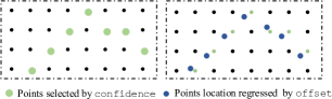
Figure 2: Example of confidence and semantics in post-process. (a) The confidence is used to predict whether a keypoint is at a certain location. (b) The offset is regressed to the shift between the real keypoint and its downscaled grid. Offset is only valid in the indices with positive confidence prediction.

3 Preliminaries

3.1 Notation

In the context of lane detection models, it’s important to note that each head $i$ encompasses two distinct functions: $\mathcal{S}^{i}(\cdot)$ and $\mathcal{C}^{i}(\cdot)$. The former function yields outputs with physical significance, which we refer to as semantics. These semantics are linked to physical attributes such as distance and angle. The latter function, $\mathcal{C}^{i}(\cdot)$, produces confidence outputs for each head’s semantics. An illustration of how the post-process deals with confidence and semantics is shown in Figure 2.

Moreover, let $\mathbf{x}$ represent the vectors of unlabeled data from the calibration dataset $\mathcal{D}$. We use the symbol $\odot$ to indicate element-wise multiplication. Finally, $\hat{\mathcal{S}}$ generates new semantics derived from quantized models.

3.2 Problem Definition

Tuning-based PTQ, as mentioned in the last section, focuses on minimizing the task quantization loss as opposed to minimizing local distance, given by:

$$\min_{\mathbf{w}}\mathds{E}_{\mathbf{x}\sim\mathcal{D}}\left(\sum_{i}\left\|{\hat{\mathcal{S}}}^{i}(\mathbf{x})-\mathcal{S}^{i}(\mathbf{x})\right\|^{2}_{F}+\left\|{\hat{\mathcal{C}}}^{i}(\mathbf{x})-\mathcal{C}^{i}(\mathbf{x})\right\|^{2}_{F}\right),$$ (1)

where the first term corresponds to the reconstruction of the fully pixel-wise semantic outputs, while the second term pertains to the reconstruction of the confidence values. Compression methods (Nagel et al. 2020; Li et al. 2021) optimizes the above equation towards layer-wise and block-wise approximation.

However, such an optimization is not suitable in LD models due to their intricate post-processing steps and semantics rooted in physical interpretation. In the next section, we identify the importance of semantic sensitivity if the post-process. Thus, neglecting the valuable insights offered by post-processing in the optimization objective would ultimately yield less favorable outcomes.

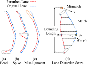
Figure 3: Common types of lane distortion caused by slight perturbation and the proposed Lane Distortion Score. (a) Bend: unexpected shifts at the terminals; (b) Spike: shifts in the middle; (c) Misalignment: missing or extra lane points. Any kind of lane distortion can be represented as a combination of those three types of distortion. (d) We measure the distortion between lanes with two types of point relationships: match and mismatch.

4 Method

In this section, we reveal an important factor that significantly impacts PTQ performance in lane detection models: the semantic sensitivity to post-processing, which has been overlooked by other PTQ research before. Then, comprehensive investigations are conducted from both intra-head and inter-head aspects. Building on sensitivity observations within and across heads, we propose a Selective Focus framework including two novel modules, Semantic Guided Focus, and Sensitivity Aware Selection, to allocate appropriate attention to different semantics. Our framework implicitly introduces the post-processing information into quantization optimization. The pipeline is depicted in Figure 1.

4.1 Semantic Sensitivity

Sensitivity to post-process

Owing to the complexity of optimizing the post-process, prevailing PTQ approaches are confined to adjusting model parameters to align quantized head outputs with their full-precision counterparts (Equation 1) without considering the post-process. Nevertheless, we find the importance of the post-process procedure in ensuring accurate lane generation. Disregarding post-processing information during the quantization optimization phase can result in pronounced distortions, including abrupt bends, spikes, and misalignments, even with a marginal value of (Equation 1), as illustrated in Figure 3.

Motivated by this, we propose to investigate semantic sensitivity, where some outputs of heads can be so important for later post-process that small quantization errors of them can cause severe lane distortion. Incorporating information from the post-process into our model optimization would pave the way for more effective semantic reconstruction.

Lane Distortion Score

To study the sensitivity, a quantitative evaluation of lane distortion becomes imperative. Given the frequently localized deviations in lanes induced by quantization (as depicted in Figure 3), we abstain from employing the conventional Intersection over Union (IoU) metric (Pan et al. 2018; Feng et al. 2022) which overlooks these local distortions. In response, a direct but effective metric is introduced, which measures the shifts of all points from the perturbed lane to the original one, as shown in Figure 3. The score of matched points is their distance, and the score of mismatched points is a fixed penalty score $v$. Concretely, our devised metric first matches points between perturbed and normal lanes (set $\mathds{M}$), then calculates the distance for matched points ($d(p_{0},p_{1})$) and the penalty from mismatched ones:

$$score=\sum_{(p_{0},p_{1})\in\mathds{M}}\frac{d(p_{0},p_{1})}{b(\mathds{M})}+nv,$$ (2)

where the bounding length normalization ($b(\mathds{M})$) is applied to accommodate lanes of varying lengths and $n$ is the number of mismatched points. More explanation of this score is available in Appendix B.

Equipped with the Lane Distortion Score, we can compute the distortion of lanes under perturbation, which strongly supports quantitively analysis of semantic sensitivity to post-process and further method design.

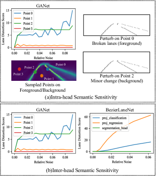
Figure 4: Illustration of semantic sensitivity. The intra-head semantic sensitivity shows that the foreground is sensitive to perturbation while the background is not. The inter-head semantic sensitivity indicates that heads are of different importance for post-processing. More illustrations are listed in the Appendix A.

4.2 Semantic Guided Focus

This section explores intra-head semantic sensitivity, where we observe that semantics within each head associated with the foreground region in post-processing play a more significant role and propose a method called Semantic Guided Focus. By leveraging confidence outputs, we can potentially discern between semantics linked to the foreground and background, which enables us to prioritize the former and obtain an improved optimization in a PTQ setting without labels.

Intra-head Semantic Sensitivity

Considering the relationship between semantics (head outputs) and the post-process, some semantics pertain to the foreground region in the post-process, while others correspond to the background. Also, it’s the distortion of the foreground region (lane) that matters. Consequently, we argue that different pixels within each head exhibit distinct sensitivities. To verify, we leverage the Lane Distortion Score of each pixel by adding the same magnitude noise to them. The results showcased in Figure 4 conclusively demonstrate that injecting noise into entries associated with the foreground region can result in more severe lane deformations. Given these findings, allocating equal attention is not reasonable during optimization.

Furthermore, it’s worth noting that the number of entries about the foreground is significantly fewer than those related to the background region, which further distracts previous techniques to focus on crucial positions. Therefore, we are motivated to enhance the accurate expression of pixels tied to the foreground region and suppress that of the background.

Intra-head Sensitivity Focus

Motivated by the findings, the core idea is to distinguish whether each element within each head will be used in the foreground region (the lane) or background.

(1) Reconstruction on semantic: We first focus on the semantic term in Equation 1 and introduce a masking function $\mathcal{M}$ to achieve the distingishment. $\mathcal{M}$ removes the error term associated with the background and retains the elements for the foreground region. Then, we incorporate them with an element-wise product, and the optimization objective on semantics becomes:

$$\mathds{E}_{\mathbf{x}\sim\mathcal{D}}\sum_{i}\left\|\mathcal{M}^{i}(\mathbf{x})\cdot(\hat{\mathcal{S}}^{i}(\mathbf{x})-\mathcal{S}^{i}(\mathbf{x}))\right\|^{2}_{F}.$$ (3)

However, due to the absence of lane annotations under the PTQ setting, it is unrealistic to identify exact elements tied to the foreground. Fortunately, we find an upper bound of Equation 3 of the models’ confidence output. Here we give the theoretical finding of this upper bound:

Theorem 1.

Given $\mathcal{M}$ representing a matrix function that discerns elements associated with foreground or background regions, and $\mathcal{C}$ denoting the confidence function of FP models, offering confidence scores for semantics linked with the foreground, the following inequation stands:

$$\mathds{E}_{\mathbf{x}\sim\mathcal{D}}\sum_{i}\left\|\mathcal{M}^{i}(\mathbf{x})\cdot(\hat{\mathcal{S}}^{i}(\mathbf{x})-\mathcal{S}^{i}(\mathbf{x}))\right\|^{2}_{F}$$ (4)

$$\leq{} \mathds{E}_{\mathbf{x}\sim\mathcal{D}}\sum_{i}\left\|\mathcal{C}^{i}(\mathbf{x})\odot(\hat{\mathcal{S}}_{i}(\mathbf{x})-\mathcal{S}^{i}(\mathbf{x}))\right\|^{2}_{F}$$

Detailed proof can be found in Appendix B. With this theorem, the semantic-related optimization target can be transformed to:

$$\min_{\mathbf{w}}\mathds{E}_{\mathbf{x}\sim\mathcal{D}}\sum_{i}\left\|\mathcal{C}^{i}(\mathbf{x})\odot(\hat{\mathcal{S}}_{i}(\mathbf{x})-\mathcal{S}^{i}(\mathbf{x}))\right\|^{2}_{F}.$$ (5)

The theorm means that we can leverage the model output $\mathcal{C}(\mathbf{x})$ as a practical proxy of the annotation mask. In intuition, the knowledge from the well-trained models can be represented in its output, thus the model could generate a mask similar to the annotation. We further assume the mask get from the model follows a binomial distribution paramterized by the confidence output, then the total expectation turns to the result in the theorem. With the upper bound from it, optimization can be more tractable.

(2) Reconstruction on confidence: Last, we incorporate the reconstruction loss on confidence values on each head. To prevent elements associated with the background region turns into the foreground, especially under large quantization noise, we propose to enhance the alignment of confidence outputs by adopting a new parameter $\lambda$ with $\lambda>1$. This heightened penalty on confidence outputs helps retain the fidelity of background-related pixels while enabling a concentrated focus on those linked to the foreground domain via the first term.

$$\min_{\mathbf{w}}\mathds{E}_{\mathbf{x}\sim\mathcal{D}}\sum_{i} (\left\|\mathcal{C}^{i}(\mathbf{x})\odot(\hat{\mathcal{S}}_{i}(\mathbf{x})-\mathcal{S}^{i}(\mathbf{x}))\right\|^{2}_{F}+$$ (6)

$$\lambda\left\|\hat{\mathcal{C}}^{i}(\mathbf{x})-\mathcal{C}^{i}(\mathbf{x})\right\|^{2}_{F}).$$

The improved Semantic Guided Focus objective indicates a simple yet elegant principle: a well-trained model inherently possesses the capacity to instruct itself. By utilizing model outputs for both mask estimation and background suppression in PTQ, the optimization process becomes foreground-oriented, leading to more efficient semantic alignment.

4.3 Sensitivity Aware Selection

We also delve into inter-head sensitivity, where we observe that specific heads are more sensitive to post-processing. This insight leads us to introduce the Sensitivity Aware Selection method, which dynamically and efficiently selects the most influential heads during PTQ reconstruction.

Inter-head Semantic Sensitivity

Considering the diverse roles played by distinct heads in post-processing, we further investigate semantic sensitivity across multiple heads. By injecting noise into each head and calculating our distortion score, Figure 4 is obtained and more results are listed in Appendix A. It can be clearly seen that under the same perturbation magnitude, certain heads like proj regression in BezierLane, exhibit notably higher Lane Distortion scores and of course correspond to severely distorted lanes, compared to others. This discrepancy highlights the considerable variation in sensitivity across different heads, which encourages us to discriminate heads and thus implicitly incorporate post-process information during optimization.

Algorithm 1 Sensitivity Aware Selection

Semantic head set $\mathds{H}$, hyper parameter $k$, and calibration dataset $\mathcal{D}$. Semantic function $\mathcal{S}(\cdot)^{i}$ and confidence functions $\mathcal{C}(\cdot)^{i}$ on head $i$ on the FP model. Quantized version $\hat{\mathcal{S}}(\cdot)^{i}$ and $\hat{\mathcal{C}}(\cdot)^{i}$.

for $\mathbf{x}\in\mathcal{D}$ do

     for $i\in\mathds{H}$ do

         Calculate full precision lanes $L$ from $\{\mathcal{S}(\mathbf{x})^{i}\}$

         Perturb the model by replacing $\mathcal{S}^{i}(\mathbf{x})$ with $\hat{\mathcal{S}}_{i}(\mathbf{x})$.

         Calculate noised lanes $\hat{L}$ from $\hat{\mathcal{S}}(\mathbf{x})^{i}$.

         Compute the $s$ of $(L,L^{\prime})$ with Equtaion 2

         Update score of $i$-th head $Score_{i}\leftarrow Score_{i}+s$

     end for

end for

Sort semantic heads by $Score$.

return Top-$k$ of semantic head set $\mathds{H}$

 Bits Method Keypoint-based Curve-based Achor-based Segmentation-based   Full Precision Model Baseline CondLaneNet GANet LSTR BézierLaneNet LaneATT SCNN RESA Small Mid Small Mid Small Mid Small Mid Small Mid Small Mid Small Mid 78.14 78.74 78.79 79.39 68.78 72.47 73.66 75.57 74.45 75.04 72.19 72.70 72.90 73.66  W8A8 ACIQ 77.95 78.58 78.58 79.21 67.50 72.14 73.43 75.36 74.34 74.56 72.03 72.55 72.76 73.64 QDrop 78.04 78.77 78.70 79.33 68.40 72.38 73.63 75.49 74.33 74.88 72.04 72.55 72.80 73.61 Ours 78.10 78.90 78.53 79.30 68.58 72.40 73.63 75.50 74.38 75.01 72.33 72.69 72.53 73.49  W8A4 ACIQ 58.63 37.67 5.38 20.18 47.63 12.49 23.79 4.77 54.20 0.64 62.63 49.26 54.16 49.62 OMSE 69.74 64.29 69.52 54.10 55.51 58.12 62.04 60.57 64.54 0.90 65.35 60.53 66.59 65.93 AdaRound 67.11 63.64 39.97 18.14 51.41 54.11 56.66 58.55 64.01 0.96 65.87 63.65 59.17 62.78 BRECQ 73.61 74.06 74.37 75.04 57.11 63.32 62.02 65.18 66.47 0.04 66.05 63.67 66.40 65.47 QDrop 74.76 75.49 75.77 75.56 60.34 65.25 64.48 66.91 66.58 0.06 66.85 64.83 67.27 67.54 Ours 75.56 75.74 76.32 76.51 63.14 68.15 68.98 70.01 69.85 34.53 69.61 69.51 69.46 70.60  W4A4 ACIQ 53.96 20.84 1.54 9.02 1.47 2.37 14.10 8.82 50.65 0.32 34.47 23.70 35.56 15.45 OMSE 63.64 55.06 49.96 37.21 1.79 17.02 52.38 46.03 62.34 0.39 51.49 49.67 57.07 50.83 AdaRound 20.35 / / / 20.69 7.95 50.70 48.60 34.53 0.00 6.56 0.03 68.36 64.57 BRECQ 74.10 75.80 75.67 75.89 30.83 50.09 66.96 70.30 68.69 28.34 54.34 52.30 67.70 69.48 QDrop 74.41 76.29 76.76 76.50 23.95 53.87 67.65 71.16 68.97 0.64 61.70 64.57 67.59 69.98 Ours 74.68 75.48 76.31 76.26 34.65 60.56 68.37 70.00 69.19 37.59 68.16 68.27 69.31 70.01  

Table 1: F1-score performance comparison among different quantization algorithms and models. W8A8 means the weight and activation are all quantized into 8 bits, and so does W4A4 and W8A4. Our method achieves superior performance under most settings.

Inter-head Sensitivity Selection

To handle varied semantic sensitivity among heads, we introduce the Sensitivity Aware Selection technique, which efficiently and adaptively selects those sensitive heads during optimization. The algorithm is formulated below and its procedure can be found in the Algorithm 1.

(1) Head selection: The noticeable differences in sensitivity prompt us to focus on the more sensitive heads, optimizing them more effectively. Naturally, given the estimated quantization noise level of each head, we can compute their own Lane Distortion Score. By ranking these scores and then selecting the top-$k$ sensitive heads, a new reconstruction loss is constructed. This approach ensures that the optimization process is cognizant of the semantic sensitivity to post-processing, leading to a better-tuned model.

(2) Adaptive selection: Moreover, the optimization process is aimed at minimizing the discrepancy between original and quantized semantics, where we recognize that the quantization loss for individual heads can evolve, leading to dynamic changes in their quantization noise levels and thus sensitivity ranking. Consequently, our selection of top-$k$ sensitive heads must adapt accordingly. In practical terms, we can reassess the Lane Distortion Scores and repeat the aforementioned step at fixed intervals of iterations. However, this repetition could impose a considerable time overhead during tuning.

(3) Efficient adaptive selection: To accelerate it, we propose to apply a pre-processing technique, which first employs the Monte-Carlo method to sample diverse noise levels and derive corresponding Lane Detection scores for each head, then interpolates sampled points from a continuous noise-score curve. This approach empowers us to gauge the semantic sensitivity of different heads based on their respective curves using their current quantization loss as queries, which introduces negligible computational burden during the optimization process. The details of building the noise-score curve are listed in Appendix B.

Based on varied semantic sensitivities across heads, we adeptly and dynamically select the most sensitive heads. This implicit inclusion of post-processing guidance leads to a better-optimized model.

5 Experiments

Extensive experiments are conducted to prove the effectiveness of the Selective Focus framework. We first present the experiment setup, and then compare the proposed method with other state-of-the-art PTQ works and the method shows up to 6.4% F1 score improvement. After that, the ablation study of the Selective Focus framework demonstrates the contribution of each component. Finally, we compare the efficiency of the framework with existing PTQ and QAT methods.

5.1 Experiments Setup

We describe the datasets and evaluation protocols, the comparison methods, and the implementation details.

Datasets and Evaluation

We conduct comprehensive experiments on the CULane dataset and adopt its official evaluation method. CULane contains 88,880 training images and 34,680 test images from multiple scenarios, and the evaluation method provides precision, recall, and F1 score for each scenario. For brevity, we list the F1 score of the whole dataset in the main document and the left in Appendix C. For models, we evaluate LD models in the four major classes: keypoint-, anchor-, segmentation-, and curve-based models, including CondLaneNet (Liu et al. 2021a), GANet (Wang et al. 2022b), LSTR (Liu et al. 2021b), BézierLaneNet (Feng et al. 2022),.LaneATT (Tabelini et al. 2021), SCNN (Pan et al. 2018), and RESA (Zheng et al. 2021).

Implementation Details

We implement our method based on the PyTorch framework. Weights and activations are both quantized with concrete bits denoted as W/A. Our method is calibrated with 512 unlabeled images on three kinds of quantization bits: W8A8, W8A4, and W4A4. During the optimization, we choose the Adam optimizer with a learning rate set as 0.000025 and adjust weights for 5000 iterations. Because of more computation overhead for layer-wise and block-wise reconstruction, the net-wise reconstruction is adopted here and wins a 6X speedup. Other hyper-parameters including $k$ for Top-$k$ in Sensitivity Aware Selection is kept as 1 for models with two heads and 2 for others, based on our ablation studies. For more detailed implementation, please refer to Appendix C.

Comparison Methods

We implement popular baselines including OMSE (Choukroun et al. 2019), ACIQ (Banner, Nahshan, and Soudry 2019), AdaRound (Nagel et al. 2020), BRECQ (Li et al. 2021), and QDrop (Wei et al. 2022). AdaRound and BRECQ are implemented by leveraging a technical advancement introduced in QDrop, achieving better results for them.

5.2 Main Results

We conduct experiments on CULane and TuSimple (TuSimple 2017) datasets. Table 1 here shows the results on CULane, and results on TuSimple are put in Appendix C due to space limit.

With the decreasing activation precision, the proposed method shows advanced performance consistently. For example, the method can achieve more than 3% up to 6.4% F1 score gain under 4-bit activation. As the noise of the semantics used in the post-process would increase significantly and the inter- and intra-head discrepancy would go worse, they may lead to degradation or even failures in methods ignoring it. Also, we note our obvious advantage in the models with specially designed feature aggregation modules, like attention in LSTR, feature flip in BézierLaneNet, and spatial convolution in SCNN and RESA. Those modules usually require information aggregated from the total network, which leads the layer-wise and block-wise methods to a harder situation, while our network-wise framework could take advantage of the cross-layer relationship naturally. Even in hard cases like LaneATT, SCNN, and RESA, the method could outperform others significantly. The proposed Selective Focus framework leverages the post-process information in the PTQ stage and thus tunes the quantized model more efficiently. With advanced performance across different precision configurations and model types, we achieve the new state-of-the-art post-training quantized lane detection and reduce the tuning time by more than 6x.

 Method Duration (Minutes) F1 Score  Ours 32 76.31 w/o Focus 31 73.27 w/o Selection 29 75.30 w/o Focus+Selection 29 72.98  

Table 2: Abalation study of the proposed framework. Each component contributes to the proposed framework, and the two components are mutually beneficial.

 Network Method Duration (Minutes) F1 Score  CondLaneNet Small [HTML]d0d0d0LSQ+ [HTML]d0d0d01303 [HTML]d0d0d076.92 QDrop 112 74.76 Ours 33 75.56  RESA Small [HTML]d0d0d0LSQ+ [HTML]d0d0d05326 [HTML]d0d0d069.80 QDrop 4378 67.59 Ours 46 69.46  

Table 3: Comparison between PTQ and QAT methods. The QAT method LSQ+ (gray region) suffers from low computation efficiency, while conventional PTQ methods such as QDrop could save the cost but with an obvious performance drop. In contrast, the proposed method significantly improve the computation efficiency with less performance gap.

5.3 Ablation Study

We first investigate the effect of each component of the proposed framework. Then, we analyze the efficiency of our method, compared to QAT and previous PTQ methods.

Component Analysis

To elucidate the contributions of individual components in our proposed method, we conducted an ablation study on GANet Small using the W4A4 quantization configuration, as detailed in Table 2. In comparison to the basic network-wise alignment (w/o Focus+Selection), our approach boosts the performance by over 3% in the F1 score. The Semantics Guided Focus emerges as the primary performance driver, underscoring the significance of foreground information and the separate reconstruction benefits for semantics and confidence. While the standalone Sensitivity Aware Selection module enhances the F1 score by a modest 0.3%, its cooperation with Focus amplifies the improvement to 1%, proving the framework’s capability to manage semantic sensitivities both within and across heads. Notably, the proposed optimization strategy achieves performance on par with block-wise PTQ, yet maintains a speed akin to network-wise reconstruction. Besides, experiments on the impact of the hyperparameters of Selection and the dynamic sensitivity property during optimization are all listed in Appendix C.

Efficiency Analysis

Although QAT comes with cost and privacy concerns, it remains the premier quantization algorithm due to its promising performance. To evaluate the performance and efficiency gap between QAT and PTQ, we performed comparative experiments on CondLaneNet and RESA, utilizing the W8A4 quantization setup. These selected models differ in computational demands, allowing us to thoroughly probe the disparities between QAT and PTQ. Besides, though block-wise PTQ methods, such as QDrop, are much faster than QAT, the storage overhead and processing time for feature maps in intermediate layers are still problems. This is also the reason that we choose the efficient network-wise reconstruction, bringing a 6x speedup.

6 Conclusion

This paper sheds light on the post-training quantization in lane detection models leveraging the inherent semantics sensitivity. Our study delves into the essence of semantic sensitivity in the post-process and proposes a novel pipeline for identifying the sensitivity and further leveraging it for optimization. By utilizing the post-processing information, the proposed framework boosts the performance of PTQ for lane detection even with the simplest optimization manner, which could motivate further exploration of the unused information lies in the lane detection models. Future endeavors might encompass efficient embedding of semantics information from post-processing—bypassing intermediate proxies more than the proposed score.

Appendix A Ilustations About Intra-head Sensitivity

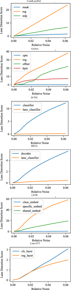
Figure 5: Illustration of inter-head semantic sensitivity of more lane detection models with more datapoints.

Many intra-head sensitivity illustrations were excluded from the main document due to space constraints. Figure 5 presents sensitivity-noise curves that provide insights into the sensitivity of post-processes to semantic errors. This figure allows for an intuitive comparison of different models under the defined Lane Distortion Score. Segmentation-based and anchor-based models exhibit greater robustness to noise. In contrast, curve-based and keypoint-based models show significant deviation in the presence of substantial noise.

Appendix B Methods

B.1 Lane Distortion Score Details

For accurate matching within the Lane Distortion Score, lanes corresponding to the points must be identified and verified. The Intersection-over-Union (IoU) of the lanes is first computed to determine if they can be paired. Once lanes are matched, we proceed from the bottom to the top of the bounding box, considering points within a 1-pixel height error as matched. Points that remain unmatched in the lanes are termed mismatched points. It is imperative to understand that this score is specifically tailored for distorted lanes; thus, its applicability is limited to lanes with similar characteristics.

B.2 Semantic Guided Focus Proof

Theorem 2.

Given $\mathcal{M}$ representing a matrix function that discerns elements associated with foreground or background regions, and $\mathcal{C}$ denoting the confidence function of FP models, offering confidence scores for semantics linked with the foreground, the following inequation stands:

$$\mathds{E}_{\mathbf{x}\sim\mathcal{D}}\sum_{i}\left\|\mathcal{M}^{i}(\mathbf{x})\cdot(\hat{\mathcal{S}}^{i}(\mathbf{x})-\mathcal{S}^{i}(\mathbf{x}))\right\|^{2}_{F}$$ (7)

$$\leq{} \mathds{E}_{\mathbf{x}\sim\mathcal{D}}\sum_{i}\left\|\mathcal{C}^{i}(\mathbf{x})\odot(\hat{\mathcal{S}}_{i}(\mathbf{x})-\mathcal{S}^{i}(\mathbf{x}))\right\|^{2}_{F}$$

Proof.

Without loss of generality, we take the $i$-th term for simplicity and denote the symbols involved as vectors.

$$\mathds{E}_{\mathbf{x}\sim\mathcal{D}}\left\|\mathcal{M}^{i}(\mathbf{x})\cdot(\hat{\mathcal{S}}^{i}(\mathbf{x})-\mathcal{S}^{i}(\mathbf{x}))\right\|^{2}_{F}$$ (8)

$$= \mathds{E}_{\mathbf{x}\sim\mathcal{D}}\sum_{j}\mathcal{M}^{i}_{j}(\mathbf{x})\cdot(\hat{\mathcal{S}}^{i}_{j}(\mathbf{x})-\mathcal{S}^{i}_{j}(\mathbf{x}))^{2}$$

$$= \sum_{j}\mathds{E}_{\mathbf{x}\sim\mathcal{D}}\mathcal{M}^{i}_{j}(\mathbf{x})\cdot\mathds{E}_{\mathbf{x}\sim\mathcal{D}}(\hat{\mathcal{S}}^{i}_{j}(\mathbf{x})-\mathcal{S}^{i}_{j}(\mathbf{x}))^{2}+$$

$$\mathrm{Cov}\left(\mathcal{M}_{j}^{i}(\mathbf{x}),\hat{\mathcal{S}}^{i}(\mathbf{x})-\mathcal{S}^{i}(\mathbf{x}))^{2}\right).$$

Similarly, the right of the equation could be expanded as

$$\mathds{E}_{\mathbf{x}\sim\mathcal{D}}\left\|\mathcal{C}^{i}(\mathbf{x})\odot(\hat{\mathcal{S}}^{i}(\mathbf{x})-\mathcal{S}^{i}(\mathbf{x}))\right\|^{2}_{F}$$ (9)

$$= \sum_{j}\mathds{E}_{\mathbf{x}\sim\mathcal{D}}\mathcal{C}^{i}_{j}(\mathbf{x})\cdot\mathds{E}_{\mathbf{x}\sim\mathcal{D}}(\hat{\mathcal{S}}^{i}_{j}(\mathbf{x})-\mathcal{S}^{i}_{j}(\mathbf{x}))^{2}+$$

$$\mathrm{Cov}\left(\mathcal{C}_{j}^{i}(\mathbf{x}),\hat{\mathcal{S}}^{i}(\mathbf{x})-\mathcal{S}^{i}(\mathbf{x}))^{2}\right).$$

Then, the goal becomes to prove

$$\mathrm{Cov}\left(\mathcal{M}_{j}^{i}(\mathbf{x}),\hat{\mathcal{S}}^{i}(\mathbf{x})-\mathcal{S}^{i}(\mathbf{x}))^{2}\right)$$ (10)

$$\leq\mathrm{Cov}\left(\mathcal{C}_{j}^{i}(\mathbf{x}),\hat{\mathcal{S}}^{i}(\mathbf{x})-\mathcal{S}^{i}(\mathbf{x}))^{2}\right).$$

Since both confidence and semantics outputs originate from the same backbone, it is inappropriate to assume their correlation. In fact, this correlation should exceed that with the mask. This observation is valid for the diagonal entries of the covariance matrix. As for the non-diagonal entries of the covariance matrix, both sides are zero due to the independency across different samples. Therefore, Equation 10 is upheld. The theorem is proved. ∎

From a sampling perspective, if the model generates an estimated mask $\hat{\mathcal{M}_{j}^{i}}$, sampled from the binomial distribution parameterized by the confidence output in each iteration, it must conform to:

$$\mathds{E}\left(\tilde{\mathcal{M}_{j}^{i}}\mid\mathbf{x}\right)=\mathcal{C}_{j}^{i}(\mathbf{x}).$$ (11)

Then the estimated expectation in the theorem could be computed with the total expectation law:

$$\mathds{E}_{\mathbf{x}\sim\mathcal{D}}\sum_{i}\left\|\tilde{\mathcal{M}}^{i}(\mathbf{x})\odot(\hat{\mathcal{S}}^{i}(\mathbf{x})-\mathcal{S}^{i}(\mathbf{x}))\right\|^{2}_{F}$$ (12)

$$= \mathds{E}_{\mathbf{x}\sim\mathcal{D}}\sum_{i}\left\|\tilde{\mathcal{M}}^{i}(\mathbf{x})\odot(\hat{\mathcal{S}}^{i}(\mathbf{x})-\mathcal{S}^{i}(\mathbf{x}))\right\|^{2}_{F}$$

$$= \mathds{E}_{\mathbf{x}\sim\mathcal{D}}\sum_{i}\mathds{E}\left(\left\|\tilde{\mathcal{M}}^{i}(\mathbf{x})\odot(\hat{\mathcal{S}}^{i}(\mathbf{x})-\mathcal{S}^{i}(\mathbf{x}))\right\|^{2}_{F}|\mathbf{x}\right)$$

$$= \mathds{E}_{\mathbf{x}\sim\mathcal{D}}\sum_{i}\left\|{\mathcal{C}}^{i}(\mathbf{x})\odot(\hat{\mathcal{S}}^{i}(\mathbf{x})-\mathcal{S}^{i}(\mathbf{x}))\right\|^{2}_{F},$$

which aligns with the intuitive notion that the model can predict a sufficiently accurate mask for the PTQ.

  CondLaneNet GANet LSTR BézierLaneNet LaneATT SCNN RESA Small Mid Small Mid Small Mid Small Mid Small Mid Small Mid Small Mid  total_tp 72486 73610 72662 75964 59547 68266 68752 69329 64173 32303 69651 70185 71701 72748 total_fn 32400 31276 32224 28922 45339 36620 36134 35557 40713 72583 35235 34701 33185 32138 total_fp 14489 16177 12367 17727 24198 27198 25785 23845 14676 49915 25582 26885 29878 28456  normal_tp 29084 29155 29116 29772 25468 27761 27939 28151 26974 14922 28687 28699 28935 29039 normal_fn 3693 3622 3661 3005 7309 5016 4838 4626 5803 17855 4090 4078 3842 3738 normal_fp 2472 2581 1907 2281 4172 3929 4060 3775 2609 14031 3383 3517 3606 3581  crowd_tp 18997 19500 19162 19937 15927 17662 17946 17940 16529 7985 18111 18217 18670 18922 crowd_fn 9006 8503 8841 8066 12076 10341 10057 10063 11474 20018 9892 9786 9333 9081 crowd_fp 4701 4850 3569 4852 7175 8333 7582 7197 4631 14178 7395 7953 8382 7927  hlight_tp 953 993 974 1090 745 953 887 965 863 373 914 920 975 932 hlight_fn 732 692 711 595 940 732 798 720 822 1312 771 765 710 753 hlight_fp 362 341 227 321 491 500 539 469 296 783 495 555 556 578  shadow_tp 2028 2016 1972 2052 1347 1706 1666 1851 1514 669 1679 1764 1729 1882 shadow_fn 848 860 904 824 1529 1170 1210 1025 1362 2207 1197 1112 1147 994 shadow_fp 368 541 373 467 898 968 1009 828 554 1382 883 839 1088 923  noline_tp 5147 5299 5278 5990 3983 5084 5122 5063 4298 2115 4891 5168 5516 5788 noline_fn 8874 8722 8743 8031 10038 8937 8899 8958 9723 11906 9130 8853 8505 8233 noline_fp 2025 2698 1890 3465 3720 5381 5219 4685 2358 6101 5792 6228 6960 6567  arrow_tp 2599 2604 2610 2697 2065 2427 2385 2457 2269 1217 2536 2541 2617 2645 arrow_fn 583 578 572 485 1117 755 797 725 913 1965 646 641 565 537 arrow_fp 271 249 198 284 515 492 545 424 304 1461 473 453 481 457  curve_tp 771 788 835 884 576 684 625 663 630 312 736 721 754 777 curve_fn 541 524 477 428 736 628 687 649 682 1000 576 591 558 535 curve_fp 176 201 120 191 305 349 359 314 212 576 283 272 363 323  cross_tp 0 0 0 0 0 0 0 0 0 0 0 0 0 0 cross_fn 0 0 0 0 0 0 0 0 0 0 0 0 0 0 cross_fp 1010 1136 1317 1881 1394 1417 1231 995 906 1936 1533 1593 2092 1764  night_tp 12907 13255 12715 13542 9436 11989 12182 12239 11096 4710 12097 12155 12505 12763 night_fn 8123 7775 8315 7488 11594 9041 8848 8791 9934 16320 8933 8875 8525 8267 night_fp 3104 3580 2766 3985 5528 5829 5241 5158 2806 9467 5345 5475 6350 6336  

Table 4: Full metrics on the CULane dataset of our method under W4A4 quantization configuration. Further precision/recall/F1 scores could be derived from those data.

Precision	Method	BezierLaneNet		GANet		LSTR		SCNN
wa88	ACIQ	94.96	95.35	97.60	95.80	93.95	94.04	92.47	94.73
w8a4	ACIQ	49.99	66.54	39.29	72.36	90.59	92.70	60.85	82.88
	OMSE	91.95	92.73	93.61	91.79	92.02	93.05	85.17	91.99
	AdaRound	92.85	93.73	92.08	90.77	94.05	94.41	80.19	89.44
	BRECQ	94.39	94.81	95.00	92.48	93.94	94.56	89.12	93.61
	QDrop	94.13	94.76	94.87	92.38	94.03	94.43	88.95	93.27
	Ours	94.88	95.27	96.60	94.78	94.75	94.63	92.31	94.66
wa44	ACIQ	48.13	65.30	19.07	58.17	4.85	45.15	48.94	77.85
	OMSE	87.89	89.88	88.71	90.75	4.59	44.67	77.36	88.69
	AdaRound	94.72	94.91	0.00	0.00	46.19	66.98	14.08	63.37
	BRECQ	94.86	95.23	95.91	94.82	77.03	87.24	67.32	85.63
	QDrop	94.54	95.07	96.24	94.50	42.61	64.44	90.37	93.82
	Ours	95.04	95.33	96.55	94.68	86.22	90.10	91.98	94.70

Table 5: TuSimple performance comparison among different quantization algorithms and models, where the first column is the F1 score and the second is the accuracy. W8A8 means the weight and activation are all quantized into 8 bits, and so does W4A4 and W8A4. Note that the 8-bit quantization has almost no performance effect on the TuSimple dataset, so we skip the training-based methods on it.

B.3 Semantic and Architectural Discrepancies in Quantization

The PTQ method, as detailed in (Liu et al. 2021c), targets discrepancies arising from architecture during the forward pass of quantized models. It identifies that the quantization of multi-head attention (MHA) modules can alter the relative order of attention maps, leading to performance deterioration. To address this, it introduces a ranking-aware loss that preserves the order across different attention heads.

Conversely, our research delves into the diverse functionalities in post-processing, highlighting task-specific variance. While prior post-training approaches concentrated on aligning activations between quantized models and their float-point counterparts, we recognize that the significance of these activations varies depending on the semantics. To the best of our knowledge, this work is the first to leverage non-differential post-processing to quantize detection models, thereby boosting both performance and efficiency.

(Liu et al. 2021c) and our work respectively focus on the intermediate outputs of MHA modules, and the network’s final outputs in terms of semantic sensitivity. This opens up the possibility of integrating these two methods for enhanced overall performance, given their non-conflicting optimization paths.

Appendix C Experiments

C.1 Implementation Details

The proposed quantization algorithms are structured into three distinct stages: (1) preparation, (2) calibration, and (3) tuning, as detailed below.

Prepare

To initiate the process, a sensitivity-noise curve for each model is established, which subsequently aids in Sensitivity Aware Selection. We randomly sample 100 images from the training dataset to act as data points. Initially, the full-precision model predicts the lanes of these images, caching outputs from every head. For each head, varying noise levels are applied to these cached outputs. Subsequently, the distorted lanes are decoded from the post-process. The Lane Distortion Scores, calculated at every noise level and data point, act as the proxy function in Sensitivity Aware Selection after being interpolated.

Network	Task	# Head	Dataset	Metric	FP	W/A	OMSE	QDrop	Ours
CenterNet	det 2d	3	COCO	bbox mAP	25.9	4/4	5.8	11.0	13.3
CondlaneNet	lane det	6	CurveLanes	F1 Score	85.1	4/4	76.9	81.4	82.8

Table 6: Abaltaion on other detection tasks and datasets.

$k$	Accuracy	F1 Score
1	89.31	91.66
2	94.66	96.46
3	94.75	96.51
4	94.60	96.23

Table 7: Abaltaion of the hyperparameter effect in the Sensitivity Aware Selection on GANet (Small) and TuSimple Dataset.

The sensitivity curve construction needs 100 unlabeled images across 8 noise levels, with 20 reruns at each level, which means every image needs 1 forward and 160 post-processes. It totals approximately 10 minutes per network — a minor cost compared to the training part.

Calibrate

For calibration, the quantized models use 512 random images from the training dataset, determining the scale (with a zero-point consistently set at 0 for symmetric quantization). The augmentation follows the full-precision models without any additional modifications. While the OMSE calibration technique is employed, an exponential moving average MSE is also utilized for activations to enhance performance. Once the scales are ascertained, they are frozen during the tuning.

Tuning

After obtaining a calibrated quantized model, we implement training-based PTQ. Mini-batches are derived from the calibration data without any further data augmentations. The target outputs are the cached head outputs from the full-precision models, whereas the optimization objective is defined in Equation (6) for the selected heads. The optimization process spans 5000 iterations, updating the selection after every 2000 iterations. With block assignment (Li et al. 2021; Wei et al. 2022) and specific tuning strategies (Nagel et al. 2020; Hubara et al. 2020; Wang et al. 2022a), our method sets a new benchmark using straightforward training configurations. This stellar performance is attributed to our well-designed methods for knowledge extraction from the post-process.

C.2 Full Metrics On The CULane Dataset

The evaluation on the CULane dataset incorporates metrics for various scenarios. We present the metrics of our W8A4 method in Table 4. A notable observation is a significant discrepancy in false positives among models, indicating that performance primarily hinges on the model’s ability to avoid misidentifying lanes under limited precision.

C.3 Extended Experiments On The TuSimple Dataset

The TuSimple dataset, comprising images from highways, consists of 3626 training images and 2782 testing images. The primary evaluation metric is accuracy. Given the straightforward nature of the dataset, most models exhibit no quantization issues at higher precisions such as 8-bit. Experiments were therefore conducted on W8A4 and W4A4 for comparison, with the results detailed in Table 5. Notably, our model consistently outperforms others, boasting improvements exceeding 1.5

C.4 Dynamic Sensitivity

An ablation study on the dynamic selection’s hyper-parameter is provided herein. With four heads in the GANet model, the top-$k$ selection was set to values 1 through 4. Table 7 demonstrates that smaller $k$ values result in underoptimization, while larger ones can cause distraction. Since our intention is to focus on the most sensitive heads, this hyperparameter must be chosen judiciously.

We also documented the relative noise levels of heads, depicted in Figure 6. Initial observations indicate that the noise level in reg and cpt heads are considerably higher, leading to their early selection. This results in an overall reduction in noise levels, possibly due to a decrease in accumulative noise from the backbone and neck. As the research progresses, noise levels equilibrate, leading to the selection of sensitive heads. Although the noise levels in some heads subsequently increase, it has a negligible impact on the post-process, underscoring the efficacy of our selection process. Two key insights emerge: (1) shared components of the model influence noise distribution among heads, and (2) once shared components are stabilized, attention can be diverted to the sensitive heads.

C.5 Generalization Abalation

This proposed principle of leveraging semantics is also applicable to other tasks and other complex datasets, due to the common semantical variances across heads. We substantiate it with empirical results in Table 6. The normal detection tasks on MS COCO (Lin et al. 2014) could be improved by 2.5% bbox mAP, showing consistent improvement. The curved lane detection on CurveLanes (Xu et al. 2020) could also be improved by 1.4% F1 Score. Lane detection’s positive region (lane) is much sparser than others (bbox, etc.), which makes the post-process more sensitive and semantics more useful.

C.6 Performance Analysis

The proposed methods incur little overhead in preparation and achieve a large speed-up. Before optimization, the sensitivity-noise curves of each model should be built. As shown in Section C.1, we just need to forward each image once and repeat noised post-processing, which takes only 10 minutes in total. In the optimization phase of post-training quantization, the proposed methods require 5k iterations in total, compared to 20k iterations per block needed by prior approaches. Semantic focus modeling is the key to efficiency and effectiveness, with a pre-processing in only 10 minutes for each model. Overall, our training is completed in under an hour, while previous methods require from two hours to days.

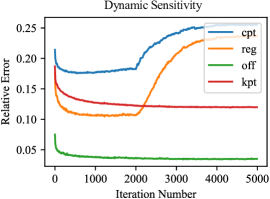
Figure 6: Dynamic noise level of GANet during its PTQ optimization with the proposed method. At the first 2k iterations, reg and cpt are chosen, and the kpt and off are chosen at the left time.

References

- Banner, Nahshan, and Soudry (2019) Banner, R.; Nahshan, Y.; and Soudry, D. 2019. Post training 4-bit quantization of convolutional networks for rapid-deployment. Advances in Neural Information Processing Systems, 32.
- Bhalgat et al. (2020) Bhalgat, Y.; Lee, J.; Nagel, M.; Blankevoort, T.; and Kwak, N. 2020. Lsq+: Improving low-bit quantization through learnable offsets and better initialization. In Proceedings of the IEEE/CVF Conference on Computer Vision and Pattern Recognition Workshops, 696–697.
- Choi et al. (2018) Choi, J.; Wang, Z.; Venkataramani, S.; Chuang, P. I.-J.; Srinivasan, V.; and Gopalakrishnan, K. 2018. Pact: Parameterized clipping activation for quantized neural networks. arXiv preprint arXiv:1805.06085.
- Choukroun et al. (2019) Choukroun, Y.; Kravchik, E.; Yang, F.; and Kisilev, P. 2019. Low-bit quantization of neural networks for efficient inference. In 2019 IEEE/CVF International Conference on Computer Vision Workshop (ICCVW), 3009–3018. IEEE.
- Esser et al. (2019) Esser, S. K.; McKinstry, J. L.; Bablani, D.; Appuswamy, R.; and Modha, D. S. 2019. Learned step size quantization. arXiv preprint arXiv:1902.08153.
- Feng et al. (2022) Feng, Z.; Guo, S.; Tan, X.; Xu, K.; Wang, M.; and Ma, L. 2022. Rethinking efficient lane detection via curve modeling. In Proceedings of the IEEE/CVF Conference on Computer Vision and Pattern Recognition, 17062–17070.
- Gong et al. (2019) Gong, R.; Liu, X.; Jiang, S.; Li, T.; Hu, P.; Lin, J.; Yu, F.; and Yan, J. 2019. Differentiable soft quantization: Bridging full-precision and low-bit neural networks. In Proceedings of the IEEE/CVF international conference on computer vision, 4852–4861.
- Hubara et al. (2020) Hubara, I.; Nahshan, Y.; Hanani, Y.; Banner, R.; and Soudry, D. 2020. Improving post training neural quantization: Layer-wise calibration and integer programming. arXiv preprint arXiv:2006.10518.
- Jacob et al. (2018) Jacob, B.; Kligys, S.; Chen, B.; Zhu, M.; Tang, M.; Howard, A.; Adam, H.; and Kalenichenko, D. 2018. Quantization and training of neural networks for efficient integer-arithmetic-only inference. In Proceedings of the IEEE conference on computer vision and pattern recognition, 2704–2713.
- Jain et al. (2020) Jain, S.; Gural, A.; Wu, M.; and Dick, C. 2020. Trained quantization thresholds for accurate and efficient fixed-point inference of deep neural networks. Proceedings of Machine Learning and Systems, 2: 112–128.
- Li et al. (2021) Li, Y.; Gong, R.; Tan, X.; Yang, Y.; Hu, P.; Zhang, Q.; Yu, F.; Wang, W.; and Gu, S. 2021. Brecq: Pushing the limit of post-training quantization by block reconstruction. arXiv preprint arXiv:2102.05426.
- Lin et al. (2014) Lin, T.-Y.; Maire, M.; Belongie, S. J.; Bourdev, L. D.; Girshick, R. B.; Hays, J.; Perona, P.; Ramanan, D.; Dollár, P.; and Zitnick, C. L. 2014. Microsoft COCO: Common Objects in Context. CoRR.
- Liu et al. (2021a) Liu, L.; Chen, X.; Zhu, S.; and Tan, P. 2021a. Condlanenet: a top-to-down lane detection framework based on conditional convolution. In Proceedings of the IEEE/CVF international conference on computer vision, 3773–3782.
- Liu et al. (2021b) Liu, R.; Yuan, Z.; Liu, T.; and Xiong, Z. 2021b. End-to-end lane shape prediction with transformers. In Proceedings of the IEEE/CVF winter conference on applications of computer vision, 3694–3702.
- Liu et al. (2021c) Liu, Z.; Wang, Y.; Han, K.; Zhang, W.; Ma, S.; and Gao, W. 2021c. Post-training quantization for vision transformer. Advances in Neural Information Processing Systems, 34: 28092–28103.
- Nagel et al. (2020) Nagel, M.; Amjad, R. A.; Van Baalen, M.; Louizos, C.; and Blankevoort, T. 2020. Up or down? adaptive rounding for post-training quantization. In International Conference on Machine Learning, 7197–7206. PMLR.
- Pan et al. (2018) Pan, X.; Shi, J.; Luo, P.; Wang, X.; and Tang, X. 2018. Spatial as deep: Spatial cnn for traffic scene understanding. In Proceedings of the AAAI Conference on Artificial Intelligence, 1.
- Qin, Wang, and Li (2020) Qin, Z.; Wang, H.; and Li, X. 2020. Ultra fast structure-aware deep lane detection. In Computer Vision–ECCV 2020: 16th European Conference, Glasgow, UK, August 23–28, 2020, Proceedings, Part XXIV 16, 276–291. Springer.
- Tabelini et al. (2021) Tabelini, L.; Berriel, R.; Paixao, T. M.; Badue, C.; De Souza, A. F.; and Oliveira-Santos, T. 2021. Keep your eyes on the lane: Real-time attention-guided lane detection. In Proceedings of the IEEE/CVF conference on computer vision and pattern recognition, 294–302.
- TuSimple (2017) TuSimple. 2017. TuSimple lane detection benchmark, 2017. https://github.com/TuSimple/tusimple-benchmark.
- Wang et al. (2022a) Wang, C.; Zheng, D.; Liu, Y.; and Li, L. 2022a. Leveraging Inter-Layer Dependency for Post -Training Quantization. In Oh, A. H.; Agarwal, A.; Belgrave, D.; and Cho, K., eds., Advances in Neural Information Processing Systems.
- Wang et al. (2022b) Wang, J.; Ma, Y.; Huang, S.; Hui, T.; Wang, F.; Qian, C.; and Zhang, T. 2022b. A keypoint-based global association network for lane detection. In Proceedings of the IEEE/CVF Conference on Computer Vision and Pattern Recognition, 1392–1401.
- Wei et al. (2022) Wei, X.; Gong, R.; Li, Y.; Liu, X.; and Yu, F. 2022. QDrop: randomly dropping quantization for extremely low-bit post-training quantization. arXiv preprint arXiv:2203.05740.
- Wu et al. (2020a) Wu, D.; Tang, Q.; Zhao, Y.; Zhang, M.; Fu, Y.; and Zhang, D. 2020a. EasyQuant: Post-training quantization via scale optimization. arXiv preprint arXiv:2006.16669.
- Wu et al. (2020b) Wu, Y.; Wu, Y.; Gong, R.; Lv, Y.; Chen, K.; Liang, D.; Hu, X.; Liu, X.; and Yan, J. 2020b. Rotation consistent margin loss for efficient low-bit face recognition. In Proceedings of the IEEE/CVF conference on computer vision and pattern recognition, 6866–6876.
- Xu et al. (2020) Xu, H.; Wang, S.; Cai, X.; Zhang, W.; Liang, X.; and Li, Z. 2020. CurveLane-NAS: Unifying Lane-Sensitive Architecture Search and Adaptive Point Blending. CoRR.
- Zheng et al. (2021) Zheng, T.; Fang, H.; Zhang, Y.; Tang, W.; Yang, Z.; Liu, H.; and Cai, D. 2021. Resa: Recurrent feature-shift aggregator for lane detection. In Proceedings of the AAAI Conference on Artificial Intelligence, 4, 3547–3554.
- Zheng et al. (2022) Zheng, T.; Huang, Y.; Liu, Y.; Tang, W.; Yang, Z.; Cai, D.; and He, X. 2022. Clrnet: Cross layer refinement network for lane detection. In Proceedings of the IEEE/CVF conference on computer vision and pattern recognition, 898–907.