Improving the Privacy Loss Under User-Level DP Composition for Fixed Estimation Error

Abstract.

This paper considers the private release of statistics of several disjoint subsets of a datasets, under user-level $\epsilon$-differential privacy (DP). In particular, we consider the user-level differentially private release of sample means and variances of speed values in several grids in a city, in a potentially sequential manner. Traditional analysis of the privacy loss due to the sequential composition of queries necessitates a privacy loss degradation by a factor that equals the total number of grids. Our main contribution is an iterative, instance-dependent algorithm, based on clipping the number of user contributions, which seeks to reduce the overall privacy loss degradation under a canonical Laplace mechanism, while not increasing the worst estimation error among the different grids. We test the performance of our algorithm on synthetic datasets and demonstrate improvements in the privacy loss degradation factor via our algorithm. We also demonstrate improvements in the worst-case error using a simple extension of a pseudo-user creation-based mechanism. An important component of this analysis is our exact characterization of the sensitivities and the worst-case estimation errors of sample means and variances incurred by clipping user contributions in an arbitrary fashion, which we believe is of independent interest.

1. Introduction

Several landmark works have demonstrated that queries about seemingly benign functions of a dataset that is not publicly available can compromise the identities of the individuals in the dataset (see, e.g., (Sweeney, 1997; Narayanan and Shmatikov, 2008)). Examples of such reconstruction attacks for the specific setting of traffic datasets, which this paper concentrates on, can be found in (Whong, 2014; Pandurangan, 2014). In this context, the framework of differential privacy (DP) was introduced in (Dwork et al., 2006), which aims to preserve the privacy of users when each user contributes at most one sample, even in the presence of additional side information. More recent work (Levy et al., 2021) considered the setting where users could contribute more than one sample and formalized the framework of user-level DP, which requires the statistical indistinguishability of the output generated by a private mechanism, where potentially all of a user’s contributions could be altered, from the output of the mechanism on the original dataset.

Now, in the traditional setting of (pure) $\epsilon$-DP or $\epsilon$-user-level DP (where $\epsilon$ captures the privacy loss), the Basic Composition Theorem shows that if the user were to pose multiple queries to the data curator in a potentially sequential (or adaptive) manner, the total privacy loss degrades by a factor that, in the worst case, equals the number of queries (see (Dwork and Roth, 2014, Cor. 3.15)). It is also well-known that there exists a differentially private mechanism, namely, the canonical Laplace mechanism, which achieves this privacy loss (see, e.g., (Steinke, 2022, Sec. 2)). We mention that in the setting where we allow for (approximate) $(\epsilon,\delta)$-DP, for a certain range of parameter values, it is possible to obtain improvements in the worst-case privacy loss as compared to that guaranteed by basic composition (Dwork and Roth, 2014, Sec. 3.5), (Dwork et al., 2010; Kairouz et al., 2017).

This paper differs in its results from other papers on composition in two respects: firstly, we consider the framework of user-level privacy; secondly, we work with pure $\epsilon$-user-level-DP and provide an algorithm that seeks to reduce the worst-case privacy loss degradation, in an instance-dependent manner, while maintaining the worst-case estimation error. Our treatment, hence, is a study of composition of user-level DP mechanisms that jointly considers the errors due to noise addition for privacy and due to the bias that results from the estimator used in the DP mechanism being different from the true function to be released. Our focus on user-level privacy assumes significance in the context of most real-world IoT datasets, such as traffic databases, which record multiple contributions from every user, with different users contributing potentially different number of samples. We mention that recent work (Arvind Rameshwar et al., 2024) presented some algorithms for real-world datasets, based on the work in (Levy et al., 2021) and (George et al., 2022), which guarantee user-level $\epsilon$-DP, and also provided theoretical proofs of their performance trends.

Our main contribution in this work is the development of a simple, yet novel, iterative algorithm, for improving the overall privacy loss under composition of several user-level DP mechanisms, each of which releases the sample mean and variance of speed records in a particular grid in a city. Our algorithm achieves the claimed improvement in privacy loss by suppressing the contributions of selected users in selected grids, while not increasing the largest worst-case error across all the grids. Crucial components of the design of our algorithm are exact characterizations of the sensitivity of the sample variance and the worst-case errors (over all datasets) in the estimation of the sample mean and variance of each grid, when the contributions of some users have been suppressed. Furthermore, the exact user-level sensitivity of the sample variance computed in this work yields, as a corollary, a strict improvement over the bound on item-level sensitivity in (Dwork et al., 2006, p. 10), which is often taken as the standard in the DP literature. With the aid of our characterizations of the worst-case errors, we suggest a simple psuedo-user creation-based algorithm—a natural extension of the work in (Arvind Rameshwar et al., 2024)—which helps reduce the worst-case estimation error. We emphasize that our algorithm can be applied more generally to the release of other statistics (potentially different from the sample mean and variance) of several disjoint subsets of the records in a dataset.

The paper is organized as follows: Section 2 presents the problem formulation and recapitulates preliminaries on DP and user-level DP. Section 3 contains a description of the mechanisms of importance to this paper and presents an exact characterization of the (user-level) sensitivity of the sample variance function. Section 4 exactly characterizes the worst-case errors in the estimation of sample mean and variance due to the suppression of selected records. Section 5 then describes our main algorithm that suppresses user contributions in an effort to improve the privacy loss under composition. We then numerically evaluate the performance of our algorithm on synthetically generated datasets in terms of the privacy loss degradation, in Section 6, and suggest a simple pseudo-user creation-based algorithm to improve the worst-case estimation error, over all grids. The paper is concluded in Section 7 with some directions for future research.

2. Preliminaries

2.1. Notation

For a given $n\in\mathbb{N}$, the notation $[n]$ denotes the set $\{1,2,\ldots,n\}$ and the notation $[a:b]$ denotes the set $\{a,a+1,\ldots,b\}$, for $a,b\in\mathbb{N}$ and $a\leq b$. Given a length-$n$ vector $\mathbf{u}\in\mathbb{R}^{n}$, we define $\lVert\mathbf{u}\rVert_{1}:=\sum_{i=1}^{n}|u_{i}|$ to be the $\ell_{1}$-norm of the vector $\mathbf{u}$. We write $X\sim P$ to denote that the random variable $X$ is drawn from the distribution $P$. We use the notation $\text{Lap}(b)$ to refer to a random variable $X$ drawn from the zero-mean Laplace distribution with standard deviation $\sqrt{2}b$; its probability distribution function (p.d.f.) obeys

$$f_{X}(x)=\frac{1}{2b}e^{-|x|/b},\ x\in\mathbb{R}.$$

2.2. Problem Setup

This work is motivated by the analysis of traffic datasets, which contain records of the data provided by IoT sensors deployed in a city, pertaining to information on vehicle movement. Each record catalogues, typically among other information, the license plate of the vehicle, the location at which the data was recorded, a timestamp, and the actual data value itself, which is the speed of the bus. Most data analysis tasks on such datasets proceed as follows: first, in an attempt to obtain fine-grained information about the statistics of the speed samples in different areas of the city, the total area of the city is divided into hexagon-shaped grids (see, e.g., Uber’s Hexagonal Hierarchical Spatial Indexing System (h3, Inc), which provides an open-source library for such partitioning tasks). Next, the timestamps present in the data records are quantized (or binned) into timeslots of fixed duration (say, one hour). In this work, we seek to release the sample averages and sample variances of speeds of vehicles in all the grids that the city area has been divided into, privately (and potentially adaptively), to a client who has no prior knowledge of these values. We remark that the algorithms discussed in this paper are readily applicable to general spatio-temporal IoT datasets with bounded data samples, for releasing other differentially private statistics.

2.3. Problem Formulation

Let $\mathcal{L}$ denote the collection of all users (or equivalently, distinct license plates) in the city, and let $\mathcal{G}$ be the collection of grids that the city area has been divided into. We set $L:=|\mathcal{L}|$ and $G:=|\mathcal{G}|$. Furthermore, for each user $\ell\in\mathcal{L}$ and each grid $g\in\mathcal{G}$, we let ${}^{g}m_{\ell}$ denote the (non-negative integer) number of speed samples contributed by user $\ell$ in the records corresponding to grid $g$. Now, for a given user $\ell\in\mathcal{L}$, let $m_{\ell}:=\sum_{g\in\mathcal{G}}{}^{g}m_{\ell}$ be the total number of speed samples contributed by user $\ell$ across all grids. Next, for every grid $g\in\mathcal{G}$, let

$${}^{g}\!\mathcal{L}:=\{\ell\in\mathcal{L}:\ {}^{g}m_{\ell}>0\}$$

be the collection of users whose contributions constitute the data records corresponding to grid $g$. We let ${}^{g}m^{\star}$ (resp. ${}^{g}m_{\star}$) denote the largest (resp. smallest) number of samples contributed by any user in grid $g\in\mathcal{G}$. Formally, ${}^{g}m^{\star}=\max_{\ell\in{}^{g}\!\mathcal{L}}{}^{g}m_{\ell}$, and ${}^{g}m_{\star}=\min_{\ell\in{}^{g}\!\mathcal{L}}{}^{g}m_{\ell}$. For every user $\ell\in\mathcal{L}$, let

$$\mathcal{G}_{\ell}:=\{g\in\mathcal{G}:\ {}^{g}m_{\ell}>0\}$$

be the collection of grids whose records user $\ell$ contributes to. In line with the previous notation, we set ${}^{g}L:=|{}^{g}\!\mathcal{L}|$ and $G_{\ell}:=|\mathcal{G}_{\ell}|$. Throughout this paper, we assume, without loss of generality, that $G_{1}\geq G_{2}\geq\ldots\geq G_{L}$.

Now, let ${}^{g}S_{\ell}$ denote the vector of speed samples contributed by user $\ell\in\mathcal{L}$ in grid $g\in\mathcal{G}$; more precisely, ${}^{g}S_{\ell}:=\left({}^{g}S_{\ell}^{(j)}:\ j\in\left[{}^{g}m_{\ell}\right]\right)$. We assume that each ${}^{g}S_{\ell}^{(j)}$ is a non-negative real number that lies in the interval $[0,U]$, where $U$ is a fixed upper bound on the speeds of the vehicles. For the real-world datasets that are the objects of consideration in this paper, the speed samples are drawn according to some unknown distribution $P$ that is potentially non-i.i.d. (independent and identically distributed) across samples and users. Our analysis is distribution-free in that we work with the worst-case errors in estimation over all datasets, in place of distribution-dependent error metrics such as the expected error (see, e.g., (Kamath and Ullman, 2020, Sec. 1.1) for a discussion).

We call the dataset consisting of the speed records contributed by users as

$$\mathcal{D}=\left\{\left(\ell,\left\{{}^{g}S_{\ell}:g\in\mathcal{G}\right\}\right):\ell\in\mathcal{L}\right\}.$$

We let $\mathsf{D}$ denote the universe of all possible datasets with a given distribution of numbers of samples contributed by users across grids $\{{}^{g}m_{\ell}:\ell\in\mathcal{L},g\in\mathcal{G}\}$.

The function that we are interested in is the length-$G$ vector $f:\mathsf{D}\to(\mathbb{R}^{2})^{G}$, each of whose components is a $2$-tuple of the sample average and the sample variance of speed samples in each grid. More precisely, we have

(1) $$f(\mathcal{D})=\left({}^{g}\!f(\mathcal{D}):g\in\mathcal{G}\right),$$

where ${}^{g}\!f:\mathsf{D}\to\mathbb{R}^{2}$ is such that

(2) $${}^{g}\!f(\mathcal{D})=\begin{bmatrix}{}^{g}\!\mu(\mathcal{D})\\ {}^{g}\textsf{Var}(\mathcal{D})\end{bmatrix}.$$

Here,

(3) $${}^{g}\!\mu(\mathcal{D}):=\frac{1}{\sum\limits_{\ell\in{{}^{g}\!\mathcal{L}}}{}^{g}m_{\ell}}\cdot\sum_{\ell\in{{}^{g}\!\mathcal{L}}}\sum_{j=1}^{{}^{g}m_{\ell}}{}^{g}S_{\ell}^{(j)}$$

is the sample mean of speed records in grid $g$ and

(4) $${}^{g}\textsf{Var}(\mathcal{D})=\frac{1}{\sum_{\ell\in{}^{g}\!\mathcal{L}}{}^{g}m_{\ell}}\cdot\sum_{\ell\in{}^{g}\!\mathcal{L}}\sum_{j=1}^{{}^{g}m_{\ell}}\left({}^{g}S_{\ell}^{(j)}-{}^{g}\!\mu(\mathcal{D})\right)^{2}$$

is the sample variance of speed records in grid $g$. For the purposes of this work, one can equivalently think of $f(\mathcal{D})$ as a length-$2G$ vector, each of whose components is a scalar mean or variance. A central objective in user-level differential privacy is the private release of an estimate of $f$, without compromising too much on the accuracy in estimation. We next recapitulate the definition of user-level differential privacy (Levy et al., 2021).

2.4. User-Level Differential Privacy

Consider two datasets $\mathcal{D}_{1}=\left\{\left({\ell},\left\{{}^{g}x_{\ell}:g\in\mathcal{G}\right\}\right):\ \ell\in\mathcal{L}\right\}$ and   $\mathcal{D}_{2}=$ $\left\{\left(\ell,\left\{{}^{g}\tilde{x}_{\ell}:g\in\mathcal{G}\right\}\right):\ \ell\in\mathcal{L}\right\}$ consisting of the same users, with each user contributing the same number of (potentially different) data values. Recall that $\mathsf{D}$ is the universal set of such databases. We say that $\mathcal{D}_{1}$ and $\mathcal{D}_{2}$ are “user-level neighbours” if there exists $\ell_{0}\in[L]$ such that $\left\{{}^{g}x_{\ell_{0}}:g\in\mathcal{G}\right\}\neq\left\{{}^{g}\tilde{x}_{\ell_{0}}:g\in\mathcal{G}\right\}$, with $\left\{{}^{g}x_{\ell}:g\in\mathcal{G}\right\}=\left\{{}^{g}\tilde{x}_{\ell}:g\in\mathcal{G}\right\}$, for all $\ell\neq\ell_{0}$. Clearly, datasets $\mathcal{D}_{1}$ and $\mathcal{D}_{2}$ differ in at most $m_{\ell_{0}}$ samples, where $m_{\ell_{0}}\leq m^{\star}$, where $m^{\star}:=\max_{\ell\in\mathcal{L}}m_{\ell}$.

Definition 2.0.

For a fixed $\varepsilon>0$, a mechanism $M:\mathsf{D}\to\mathbb{R}^{d}$ is said to be user-level $\varepsilon$-DP if for every pair of datasets $\mathcal{D}_{1},\mathcal{D}_{2}$ that are user-level neighbours, and for every measurable subset $Y\subseteq\mathbb{R}^{d}$, we have that

$$\Pr[M(\mathcal{D}_{1})\in Y]\leq e^{\varepsilon}\Pr[M(\mathcal{D}_{2})\in Y].$$

Next, we recall the definition of the user-level sensitivity of a function of interest.

Definition 2.0.

Given a function $\theta:\mathsf{D}\to\mathbb{R}^{d}$, we define its user-level sensitivity $\Delta_{\theta}$ as

$$\Delta_{\theta}:=\max_{\mathcal{D}_{1},\mathcal{D}_{2}\ \text{u-l nbrs.}}\left\lVert\theta(\mathcal{D}_{1})-\theta(\mathcal{D}_{2})\right\rVert_{1},$$

where the maximization is over datasets that are user-level neighbours.

In this paper, we use the terms “sensitivity” and “user-level sensitivity” interchangeably. The next result is well-known and follows from standard DP results (Dwork et al., 2006, Prop. 1):

Theorem 2.3.

For a function $\theta:\mathsf{D}\to\mathbb{R}^{d}$, the mechanism $M^{\text{Lap}}:\mathsf{D}\to\mathbb{R}^{d}$ defined by

$$M^{\text{Lap}}(\mathcal{D})=\theta(\mathcal{D})+Z,$$

where $Z=(Z_{1},\ldots,Z_{d})$ is such that $Z_{i}\sim\text{Lap}(\Delta_{\theta}/\varepsilon)$, is user-level $\varepsilon$-DP.

Furthermore, by standard results on the tail probabilities of Laplace random variables, we obtain the following bound on the estimation error due to the addition of noise for privacy:

Proposition 2.0.

For a given function $\theta:\mathsf{D}\to\mathbb{R}^{d}$ and for any dataset $\mathcal{D}_{1}$, we have that

$$\Pr\left[\left\lVert M^{\text{Lap}}(\mathcal{D}_{1})-\theta(\mathcal{D}_{1})\right\rVert_{1}\geq\frac{\Delta_{\theta}\ln(1/\delta)}{\varepsilon}\right]\leq\delta,$$

for all $\delta\in(0,1]$.

In the following subsection, we shall discuss the overall privacy loss that results from the composition of several user-level $\epsilon$-DP mechanisms together.

2.5. Composition of User-Level DP Mechanisms

Recall that our objective in this work is the (potentially sequential, or adaptive) release of a fixed function (in particular, the sample mean and sample variance) of the records in each grid, over all grids. The following fundamental theorem from the DP literature (Dwork and Roth, 2014, Cor. 3.15) captures the worst-case privacy loss degradation upon composition of (user-level) DP mechanisms. For each $g\in\mathcal{G}$, let ${}^{g}M:\mathsf{D}\to\mathbb{R}^{d}$ be an ${}^{g}\epsilon$-DP algorithm that acts exclusively on those records from grid $g$. Further, let $M=\left({}^{g}M:\ g\in\mathcal{G}\right)$ be the composition of the $G$ mechanisms above.

Theorem 2.5 (Basic Composition Theorem).

We have that $M$ is user-level $\sum_{g\in\mathcal{G}}{}^{g}\epsilon$-DP.

It is well-known (see, e.g., (Steinke, 2022, Sec. 2.1)) that Theorem 2.5 is tight, in that there exists a Laplace mechanism (of the form in Theorem 2.3) that achieves a privacy loss of $\sum_{g\in\mathcal{G}}{}^{g}\epsilon$ upon composition.

Observe from Theorem 2.5 that in the case when ${}^{g}\epsilon=\epsilon$, for all $g\in\mathcal{G}$, we obtain an overall privacy loss of $G\epsilon$, upon composition. Clearly, when the number of grids $G$ is large, the overall privacy loss is large, as well.

We next present a simple improvement of the Basic Composition Theorem above that takes into account the fact that each mechanism ${}^{g}M$, for $g\in\mathcal{G}$, acts only on the records in the grid $g$. Let $\overline{\epsilon}:=\max_{\ell\in\mathcal{L}}\sum_{g\in\mathcal{G}_{\ell}}{}^{g}\epsilon$.

Theorem 2.6.

We have that $M$ is user-level $\overline{\epsilon}$-DP.

Proof.

Consider datasets $\mathcal{D}$ and $\mathcal{D}^{\prime}$ that differ (exclusively) in the contributions of user $\ell\in\mathcal{L}$. Now, consider any measurable set $T=\left({}^{1}T,\ldots,{}^{G}T\right)\subseteq\mathbb{R}^{G}$. For ease of reading, we let ${}^{(g-1)}M(\mathcal{D}):=({}^{1}M(\mathcal{D}),\ldots,{}^{g-1}M(\mathcal{D})))$; likewise, we let ${}^{(g-1)}T:=({}^{1}T,\ldots,{}^{g-1}T)$.

$$\frac{\Pr[M(\mathcal{D})\in T]}{\Pr[M(\mathcal{D}^{\prime})\in T]}$$

$$=\frac{\prod_{g\in\mathcal{G}}\Pr[{}^{g}M(\mathcal{D})\in{}^{g}T|{}^{(g-1)}M(\mathcal{D})\in{}^{(g-1)}T]}{\prod_{g\in\mathcal{G}}\Pr[{}^{g}M(\mathcal{D}^{\prime})\in{}^{g}T|{}^{(g-1)}M(\mathcal{D}^{\prime})\in{}^{(g-1)}T]}$$

$$\leq e^{\sum_{g\in\mathcal{G}_{\ell}}{}^{g}\epsilon},$$

where the last inequality follows from the DP property of each mechanism ${}^{g}M$, $g\in\mathcal{G}$. The result then follows immediately. ∎

As a simple corollary, from our assumption that $G_{1}\geq G_{2}\geq\ldots\geq G_{L}$, we obtain the following result:

Corollary 2.0.

When ${}^{g}\epsilon=\epsilon$, for all $g\in\mathcal{G}$, we have that $M$ is $G_{1}\epsilon$-DP.

In what follows, we shall focus on this simplified setting where the privacy loss ${}^{g}\epsilon$ for each grid $g$ is fixed to be $\epsilon>0$. Note that if $G_{1}$ is large, the privacy loss upon composing the mechanisms corresponding to the different grids of the city is correspondingly large.

A natural question that arises, hence is: can we improve the worst-case privacy loss (in the sense of Corollary 2.7) in such a manner as to preserve some natural notion of the worst-case error over all grids? In what follows, we shall show that for a specific class of (canonical) mechanisms, a notion of the worst-case error over all grids can be made precise, which will then serve as a guideline for the design of our algorithm that improves the privacy loss degradation by clipping user contributions.

We end this subsection with a remark. In the setting of item-level DP, where each user contributes at most one sample, it follows from Theorem 2.7 that the composition of mechanisms that act on disjoint subsets of a dataset has the same privacy loss as that of any individual mechanism, i.e., $M$ is $\epsilon$-DP as well. In such a setting, it is not possible to improve on the privacy loss degradation by clipping user contributions.

The next section describes the mechanisms that will be of use in this paper; we refer the reader to (Levy et al., 2021; Arvind Rameshwar et al., 2024) for more user-level DP mechanisms for releasing sample means and their performance on real-world datasets.

3. Mechanisms for Releasing DP Estimates

In this section and the next, we focus our attention on a single grid $g\in\mathcal{G}$. For notational simplicity, we shall drop the explicit dependence of the notation (via superscripts) in Section 2 on $g$; alternatively, it is instructive to consider this setting as a special case of the setting in Section 2, where $|\mathcal{G}|=1$. In particular, ${}^{g}m_{\ell}=m_{\ell}$, for all $\ell\in\mathcal{L}$, ${}^{g}\!\mathcal{L}=\mathcal{L}$, and ${}^{g}\!\mu=\mu$ and ${}^{g}\textsf{Var}=\textsf{Var}$. With some abuse of notation, we let $\mathcal{D}$ denote the dataset consisting of records in grid $g$ and let $\mathsf{D}$ denote the universal set of datasets with the distribution $\{m_{\ell}\}$ of user contributions.

We now describe two mechanisms for releasing user-level differentially private estimates of the sample mean and variance of a single grid.

3.1. Baseline

Given the definitions $\mu$ and Var as in (3) and (4), the first mechanism, which we call Baseline, simply adds the right amount of Laplace noise to $\mu$ and Var to ensure user-level $\epsilon$-DP. Formally, the Baseline mechanism $M_{\text{b}}:\mathsf{D}\to\mathbb{R}^{2}$ obeys

$$M_{\text{b}}(\mathcal{D})=\begin{bmatrix}M_{\mu,\text{b}}(\mathcal{D})\\ M_{\textsf{Var},\text{b}}(\mathcal{D})\end{bmatrix},$$

where

$$M_{\mu,\text{b}}(\mathcal{D})=\mu(\mathcal{D})+\text{Lap}(2\Delta_{\mu}/\varepsilon),$$

and

$$M_{\textsf{Var},\text{b}}(\mathcal{D})=\textsf{Var}(\mathcal{D})+\text{Lap}(2\Delta_{\textsf{Var}}/\varepsilon).$$

Note that the privacy budget for the release of each of the sample mean and variance is fixed to $\epsilon/2$, leading to $M_{\text{b}}$ being $\epsilon$-user-level DP, overall, by Theorem 2.5. Furthermore, from the definition of user-level sensitivity in Section 2, we have that

(5) $$\Delta_{\mu}=\frac{U\cdot\max_{\ell\in\mathcal{L}}m_{\ell}}{\sum\limits_{\ell\in{\mathcal{L}}}{m_{\ell}}}=\frac{U\cdot m^{\star}}{\sum\limits_{\ell\in{\mathcal{L}}}m_{\ell}}.$$

An explicit computation of the user-level sensitivity of Var, however, requires significantly more effort. The next proposition, whose proof is provided in Appendix A exactly identifies $\Delta_{\textsf{Var}}$.

Proposition 3.0.

We have that

$$\Delta_{\textsf{Var}}=\begin{cases}\frac{U^{2}\ m^{\star}(\sum_{\ell}m_{\ell}-m^{\star})}{\left(\sum_{\ell}m_{\ell}\right)^{2}},\ \text{if }\sum_{\ell}m_{\ell}>2m^{\star},\\ \frac{U^{2}}{4},\ \text{if $\sum_{\ell}m_{\ell}\leq 2m^{\star}$ and $\sum_{\ell}m_{\ell}$ is even},\\ \frac{U^{2}}{4}\cdot\left(1-\frac{1}{(\sum_{\ell}m_{\ell})^{2}}\right),\ \text{if $\sum_{\ell}m_{\ell}\leq 2m^{\star}$ and $\sum_{\ell}m_{\ell}$ is odd}.\end{cases}.$$

We then obtain the following corollary on the sensitivity of the sample variance function in the item-level DP setting where each user contributes exactly one sample, i.e., when $m_{\ell}=1$, for all $\ell\in\mathcal{L}$.

Corollary 3.0.

In the setting of item-level DP, we have

$$\Delta_{\textsf{Var}}=\begin{cases}\frac{U^{2}(L-1)}{L^{2}},\ \text{if }L\geq 2,\\ 0,\ \text{if $L=1$}.\end{cases}.$$

On the other hand, the well-known upper bound on the sensitivity of the sample variance in (Dwork et al., 2006, p. 10) that is now standard for DP applications shows that in the item-level DP setting, $\Delta_{\textsf{Var}}\leq 8U^{2}/L$. Clearly, the exact sensitivity computed in Corollary 3.2 is a strict improvement over this bound, by a multiplicative factor of more than $8$, for all $L$.

Now, consider the expression in Proposition 3.1 above, for a fixed $\sum_{\ell}m_{\ell}$. Suppose also that $\sum_{\ell}m_{\ell}>2m^{\star}$. Hence, for this range of $m^{\star}$ values, it is easy to argue that $h(m^{\star}):=m^{\star}(\sum_{\ell}m_{\ell}-m^{\star})$ is increasing in $m^{\star}$, implying that for a fixed value of $\sum_{\ell}m_{\ell}$, we have that $\Delta_{\textsf{Var}}$ is increasing in $m^{\star}$, in the regime where $\sum_{\ell}m_{\ell}>2m^{\star}$. Furthermore, it is easy to argue that $\Delta_{\textsf{Var}}\leq U^{2}/4$, for all values of $\{m_{\ell}\}$, implying that $\Delta_{\textsf{Var}}$ is non-decreasing, overall, as $m^{\star}$ increases. In other words, a large value of $m^{\star}$ leads to a large sensitivity. In our next mechanism, which we call Clip, we attempt to ameliorate this issue by clipping the number of contributions of each user in the grid, at the cost of some error in accuracy.

3.2. Clip

We proceed to describe a simple modification of the previous mechanism, which we call Clip, for releasing user-level differentially private estimates of $\mu$ and Var, by clipping (or suppressing) selected records. For $\ell\in\mathcal{L}$, we let $\Gamma_{\ell}\in[0:m_{\ell}]$ denote the number of contributions of user $\ell$ that have not been clipped; without loss of generality, we assume that the set of indices of these samples is $[\Gamma_{\ell}]$. Further, we assume that $\sum_{\ell}\Gamma_{\ell}>0$. We use the notation $\Gamma^{\star}:=\max_{\ell\in\mathcal{L}}\Gamma_{\ell}$.

Given the dataset $\mathcal{D}$, we set

(6) $$\mu_{\text{clip}}(\mathcal{D})=\frac{1}{\sum_{\ell}\Gamma_{\ell}}\cdot\sum_{\ell=1}^{L}\sum_{j=1}^{\Gamma_{\ell}}S_{\ell}^{(j)}$$

to be that estimator of the sample mean that is obtained by retaining only $\Gamma_{\ell}$ samples, for each user $\ell$. Next, we set

(7) $$\textsf{Var}_{\text{clip}}(\mathcal{D})=\frac{1}{\sum_{\ell}\Gamma_{\ell}}\cdot\sum_{\ell=1}^{L}\sum_{j=1}^{\Gamma_{\ell}}\left(S_{\ell}^{(j)}-\mu_{\text{clip}}(\mathcal{D})\right)^{2}$$

to be an estimator of the sample variance that makes use of the previously computed estimator $\mu_{\text{clip}}(\mathcal{D})$ of the sample mean.

Our mechanism $M_{\text{clip}}:\mathsf{D}\to\mathbb{R}^{2}$ obeys

(8) $$M_{\text{clip}}(\mathcal{D})=\begin{bmatrix}M_{\mu,\text{clip}}(\mathcal{D})\\ M_{\textsf{Var},\text{clip}}(\mathcal{D})\end{bmatrix},$$

where

$$M_{\mu,\text{clip}}(\mathcal{D})=\mu_{\text{clip}}(\mathcal{D})+\text{Lap}(2\Delta_{\mu_{\text{clip}}}/\varepsilon),$$

and

$$M_{\textsf{Var},\text{clip}}(\mathcal{D})=\textsf{Var}_{\text{clip}}(\mathcal{D})+\text{Lap}(2\Delta_{\textsf{Var}_{\text{clip}}}/\varepsilon).$$

Here, $\Delta_{\mu_{\text{clip}}}$ and $\Delta_{\textsf{Var}_{\text{clip}}}$ are respectively the user-level sensitivities of the clipped mean estimator $\mu_{\text{clip}}$ and the clipped variance estimator $\textsf{Var}_{\text{clip}}$. As before, we assign a privacy budget of $\epsilon/2$ for each of the mechanisms $M_{\mu,\text{clip}}$ and $M_{\textsf{Var},\text{clip}}$. Clearly, both these algorithms are $\varepsilon/2$-user-level DP, from Theorem 2.3, resulting in the overall mechanism $M_{\text{clip}}$ being $\epsilon$-user-level DP, from Theorem 2.5.

By arguments similar to those in (Arvind Rameshwar et al., 2024, Sec. III.C), we have that

(9) $$\Delta_{\mu_{\text{clip}}}=\frac{U\ \Gamma^{\star}}{\sum_{\ell=1}^{L}\Gamma_{\ell}}.$$

Furthermore, by analysis entirely analogous to the proof of Proposition 3.1, we obtain the following lemma:

Lemma 3.0.

We have that

$$\Delta_{\textsf{Var}_{\text{clip}}}=\begin{cases}\frac{U^{2}\ \Gamma_{\ell}^{\star}(\sum_{\ell}\Gamma_{\ell}-\Gamma_{\ell}^{\star})}{\left(\sum_{\ell}\Gamma_{\ell}\right)^{2}},\ \text{if }\sum_{\ell}\Gamma_{\ell}>2\Gamma^{\star},\\ \frac{U^{2}}{4},\ \text{if $\sum_{\ell}\Gamma_{\ell}\leq 2\Gamma^{\star}$ and $\sum_{\ell}\Gamma_{\ell}$ is even},\\ \frac{U^{2}}{4}\cdot\left(1-\frac{1}{(\sum_{\ell}\Gamma_{\ell})^{2}}\right),\ \text{if $\sum_{\ell}\Gamma_{\ell}\leq 2\Gamma^{\star}$ and $\sum_{\ell}\Gamma_{\ell}$ is odd}.\end{cases}$$

In Appendix B, we show that for a special class of clipping strategies considered in (Arvind Rameshwar et al., 2024), the sensitivities $\Delta_{\mu_{\text{clip}}}$ and $\Delta_{\textsf{Var}_{\text{clip}}}$ are in fact at most the values of their Baseline counterparts $\Delta_{\mu}$ and $\Delta_{\textsf{Var}}$, respectively. We mention that the mechanisms $M_{\mu,\text{clip}}$ and $M_{\textsf{Var},\text{clip}}$ are also called as pseudo-user creation-based mechanisms, in this case.

In the next section, we focus more closely on the Clip mechanism and explicitly characterize the worst-case errors (over all datasets) due to clipping the contributions of users.

4. Worst-Case Errors in Estimation of Sample Mean and Variance

In this section, we continue to focus on a single grid $g\in\mathcal{G}$ and explicitly identify the worst-case error due to clipping incurred, over all datasets, by the Clip mechanism with an arbitrary choice $\Gamma_{\ell}\in[0:m_{\ell}]$, for $\ell\in\mathcal{L}$. The characterizations of worst-case errors in this section will be of use in the design of our algorithm for improving the privacy loss degradation under composition, via the clipping (or suppression) of user contributions in selected grids. We now make the notion of the worst-case clipping error formal.

Consider the functions $\mu,\textsf{Var}$ that stand for the true sample mean and variance, and the functions $\mu_{\text{clip}},\textsf{Var}_{\text{clip}}$ that stand for the sample mean and variance of the clipped samples, for some fixed values $\Gamma_{\ell}\in[0:m_{\ell}]$, where $\ell\in\mathcal{L}$. We now define

$$E_{\mu}(\mathcal{D}):=\lvert\mu(\mathcal{D})-\mu_{\text{clip}}(\mathcal{D})\rvert,$$

as the clipping error (or bias) for the mean on dataset $\mathcal{D}$, and

$$E_{\mu}:=\max_{\mathcal{D}\in\mathsf{D}}E_{\mu}(\mathcal{D})$$

as the worst-case clipping error for the mean. Likewise, we define

$$E_{\textsf{Var}}(\mathcal{D}):=\lvert\textsf{Var}(\mathcal{D})-\textsf{Var}_{\text{clip}}(\mathcal{D})\rvert,$$

as the clipping error for the variance on dataset $\mathcal{D}$, and

$$E_{\textsf{Var}}:=\max_{\mathcal{D}\in\mathsf{D}}E_{\textsf{Var}}(\mathcal{D})$$

as the worst-case clipping error for the variance. The following theorem from (Arvind Rameshwar et al., 2024) then holds:

Theorem 4.1 (Lemma V.1 in (Arvind Rameshwar et al., 2024)).

We have that

$$E_{\mu}=U\cdot\left(1-\frac{\sum_{\ell}\Gamma_{\ell}}{\sum_{\ell}m_{\ell}}\right).$$

In what follows, we characterize exactly the worst-case error for the variance.

Theorem 4.2.

We have that $E_{\textsf{Var}}=0$ if  $\Gamma_{\ell}=m_{\ell}$, for all $\ell\in\mathcal{L}$. Furthermore, if $\sum_{\ell}\Gamma_{\ell}<\sum_{\ell}m_{\ell}$, we have

$$E_{\textsf{Var}}=\begin{cases}\frac{U^{2}\cdot\sum_{\ell}\Gamma_{\ell}\cdot\sum_{\ell^{\prime}}(m_{\ell^{\prime}}-\Gamma_{\ell^{\prime}})}{\left(\sum_{\ell}m_{\ell}\right)^{2}},\ \text{if }\sum_{\ell}m_{\ell}>2\sum_{\ell}\Gamma_{\ell},\\ \frac{U^{2}}{4},\ \text{if $\sum_{\ell}m_{\ell}\leq 2\sum_{\ell}\Gamma_{\ell}$ and $\sum_{\ell}m_{\ell}$ is even},\\ \frac{U^{2}}{4}\cdot\left(1-\frac{1}{(\sum_{\ell}m_{\ell})^{2}}\right),\ \text{if\ $\sum_{\ell}m_{\ell}\leq 2\sum_{\ell}\Gamma_{\ell}$ and $\sum_{\ell}m_{\ell}$ is odd}.\end{cases}$$

The proof of Theorem 4.2 is provided in Appendix C.

5. An Error Metric and an Algorithm for Controlling Privacy Loss

In this section, we return to our original problem of releasing the sample means and variances of different grids in the city, possibly sequentially. We present our algorithm that seeks to control the privacy loss of a certain user-level DP mechanism for jointly releasing the sample mean and variance of all grids in the city, by clipping user contributions. As we shall see, the individual mechanisms for each grid simply add a suitable amount of Laplace noise that is tailored to the sensitivity of the functions in the grid post clipping. Our algorithm hence crucially relies on the analyses of the sensitivity and the worst-case clipping error of the Clip mechanism in Sections 3.2 and 4.

5.1. An Error Metric for Worst-Case Performance

We shall first formally define a notion of the worst-case error of any mechanism $M=({}^{g}M:\ g\in\mathcal{G})$, over all datasets, and over all grids. Our algorithm will then follow naturally from these definitions.

Formally, consider a mechanism ${}^{g}M_{\theta}:\mathsf{D}\to\mathbb{R}^{d}$, for $g\in\mathcal{G}$, for the user-level differentially private release of a statistic ${}^{g}\theta:\mathsf{D}\to\mathbb{R}^{d}$ of the records in grid $g$. Suppose that ${}^{g}M_{\theta}$ obeys

(10) $${}^{g}M_{\theta}(\mathcal{D})={}^{g}\overline{\theta}(\mathcal{D})+\overline{Z},$$

for some estimate ${}^{g}\overline{\theta}$ of ${}^{g}\theta$, such that the user-level sensitivity of ${}^{g}\overline{\theta}$ is $\Delta_{{}^{g}\overline{\theta}}$. Recall that the assumption that ${}^{g}M_{\theta}$ is a noise-adding mechanism is without loss of generality. Also, in (10), we have that $\overline{Z}$ is a length-$d$ vector with $\overline{Z}_{i}\sim\text{Lap}\left(\Delta_{{}^{g}\overline{\theta}_{i}}/\epsilon\right)$, for each coordinate $i\in[d]$. Note that we work with the class of mechanisms that add Laplace noise tailored to the sensitivities of each grid, individually, since explicit computation of the user-level sensitivity of the vector $f$ in (1) (across all grids) is quite hard, thereby implying the necessity of loose bounds on the amount of noise added, when this notion of user-level sensitivity is used.

Now, consider the mechanism $M_{\theta}$ that consists of the composition of the mechanisms ${}^{g}M_{\theta}$, over $g\in\mathcal{G}$, i.e., $M_{\theta}=\left({}^{g}M_{\theta}:\ g\in\mathcal{G}\right)$. In many settings of interest, a natural error metric for such a composition of mechanisms acting on different grids is the largest worst-case estimation error among all the grids.

Now, given a mechanism ${}^{g}M_{\theta}$ as in (10), we define its worst-case estimation error as

(11) $${}^{g}E:=\sum_{i\in[d]}\max_{\mathcal{D}\in\mathsf{D}}\big{\lvert}{}^{g}\theta_{i}(\mathcal{D})-{}^{g}\overline{\theta}_{i}(\mathcal{D})\big{\rvert}+\mathbb{E}[\lVert\overline{Z}\rVert].$$

Finally, we define the error metric $E$ of the mechanism $M_{\theta}$ to be the largest worst-case estimation error among all the grids, i.e.,

$$E:=\max_{g\in\mathcal{G}}{}^{g}E.$$

We now describe our algorithm for reducing the privacy loss under composition, which makes use of a specialization of the definitions in this section to the case when the mechanisms ${}^{g}M_{\theta}$ are one of $M_{\text{b}}={}^{g}M_{\text{b}}$ (corresponding to Baseline) or $M_{\text{clip}}={}^{g}M_{\text{clip}}$ (corresponding to Clip).

5.2. An Algorithm for Clipping User Contributions

The algorithm discussed in this section results in a simple improvement of Theorem 2.5 that takes into account the structure of the queries. We mention that query-dependent composition results are also known for, say, histogram queries (see (Vadhan, 2017, Prop. 2.8)). Consider the Baseline mechanisms ${}^{g}M_{\text{b}}=\left[{}^{g}M_{\mu,\text{b}},{}^{g}M_{\textsf{Var},\text{b}}\right]^{\top}$, as defined in Section 3.1, for estimating the statistics ${}^{g}\mu$ and ${}^{g}\textsf{Var}$, for each grid $g$ of a given dataset, with $\mathsf{M}_{\text{b}}=\left({}^{g}M_{\text{b}}:\ g\in\mathcal{G}\right)$. Observe that initially, for any grid $g$, we have

$${}^{g}E =\mathbb{E}\left[\lvert\text{Lap}(2\Delta_{{}^{g}\mu}/\varepsilon)\rvert\right]+\mathbb{E}\left[\lvert\text{Lap}(2\Delta_{{}^{g}\textsf{Var}}/\varepsilon)\rvert\right]$$

(12) $$=\frac{2U\ {}^{g}m^{\star}}{\varepsilon\cdot\sum_{\ell\in\,{}^{g}\!\mathcal{L}}{}^{g}m_{\ell}}+\frac{2U^{2}\ {}^{g}m^{\star}\left(\sum_{\ell\in\,{}^{g}\!\mathcal{L}}{}^{g}m_{\ell}-{}^{g}m^{\star}\right)}{\varepsilon\cdot\left(\sum_{\ell\in\,{}^{g}\!\mathcal{L}}{}^{g}m_{\ell}\right)^{2}},$$

where the last equality follows from (5) and Proposition 3.1. As defined earlier, we have $E:=\max_{g\in\mathcal{G}}{}^{g}E.$ From Corollary 2.7, we notice that in order to improve the privacy loss upon composition, we must seek to reduce $G_{1}$, or the largest number of grids that any user “occupies”. Our aim is to accomplish this reduction in such a manner as to not increase the worst-case error $E$.

5.2.1. The Iterative Procedure

Our algorithm proceeds in stages, at each stage suppressing all the contributions of those users that occupy the largest number of grids, in selected grids that these users occupy. Clearly, since the objective is to not increase $E$, for each such user, we suppress his/her contributions in that grid which has the smallest overall (that is the sum of errors due to bias and due to the noise added for privacy; see (11)) error post suppression. We emphasize that our algorithm, being iterative in nature, is not necessarily optimal in that it does not necessarily return the lowest possible privacy loss degradation factor for a fixed worst-case error $E$. Note also that while the worst-case error (over all grids) $E$ is fixed at the start of the algorithm and is maintained as an invariant throughout its execution, the individual errors corresponding to each grid could potentially increase due to the suppression of user contributions. We let ${}^{g}E^{(0)}:={}^{g}E$, for each grid $g\in\mathcal{G}$.

For each step $t\geq 1$ in our algorithm, we pick the user(s) that occupy the largest number of grids. Define

$$\mathsf{L}^{(t)}:=\{\ell\in\mathcal{L}:\ G_{\ell}\geq G_{j},\ \forall j\in\mathcal{L}\}$$

as the set of users in the first step of our algorithm that occupy the largest number of grids. The superscript ‘$(t)$’ denotes the fact that the algorithm is in stage $t$ of its execution. Recall from our assumption that $G_{1}\geq G_{j}$, for any user $j\in\mathcal{L}$, and hence, in stage $1$, we have user $1\in\mathsf{L}^{(1)}$. We sort the users in $\mathsf{L}^{(t)}$ in increasing order of their indices, as $\ell_{1}<\ell_{2}<\ldots<\ell_{|\mathsf{L}^{(t)}|}$.

Now, for each user $\ell\in\mathsf{L}^{(t)}$, starting from user $\ell_{1}$, we calculate the worst-case error that could result in each grid he/she occupies by potentially suppressing his/her contributions entirely. More precisely, for each grid $g\in\mathcal{G}_{\ell}$, we set ${}^{g}m_{\ell}=0$, and recompute the values of $\Delta_{{}^{g}\mu}$ and $\Delta_{{}^{g}\textsf{Var}}$. In particular, following the definitions in Section 3.2, we note that after clipping in grid $g$, we have ${}^{g}\Gamma_{\ell}=0$ and ${}^{g}\Gamma_{\ell^{\prime}}=m_{\ell}$, for $\ell^{\prime}\neq\ell$, with ${}^{g}\Gamma^{\star}=\max\limits_{\ell^{\prime}\in\,{}^{g}\!\mathcal{L}:\ \ell^{\prime}\neq\ell}{}^{g}m_{\ell^{\prime}}$. Thus, (5) and Proposition 3.1, can be used to compute the sensitivities of the new sample mean and sample variance in grid $g$, which we denote as ${}^{g}\Delta_{\mu_{\text{clip}}}(\ell)$ and ${}^{g}\Delta_{\textsf{Var}_{\text{clip}}}(\ell)$, respectively.

Moreover, such a clipping of the contributions of user $\ell\in\mathsf{L}^{(1)}$ in grid $g$ introduces some worst-case clipping errors in the computation of $\mu$ and Var, which we call ${}^{g}E_{\mu}(\ell)$ and ${}^{g}E_{\textsf{Var}}(\ell)$, respectively. The exact magnitude of these clipping errors incurred can be computed using Theorems 4.1 and 4.2, using the same values of ${}^{g}\Gamma_{\ell^{\prime}}$ and ${}^{g}\Gamma^{\star}$ as described above, for $\ell^{\prime}\in{}^{g}\!\mathcal{L}$. Finally, following (11), we compute the overall worst-case error in grid $g$, post the suppression of the contributions of user $\ell$ as

(13) $${}^{g}E(\ell)={}^{g}E_{\mu}(\ell)+{}^{g}E_{\textsf{Var}}(\ell)+\frac{2\ {}^{g}\Delta_{\mu_{\text{clip}}}(\ell)}{\varepsilon}+\frac{2\ {}^{g}\Delta_{\textsf{Var}_{\text{clip}}}(\ell)}{\varepsilon}.$$

After computing the worst-case errors ${}^{g}E(\ell)$ that could result in each grid $g\in\mathcal{G}_{\ell}$ due to the potential suppression of the contributions of user $\ell$ in grid $g$, we identify one grid

(14) $$\mathsf{g}(\ell)\in\operatorname*{arg\,min}_{g\in\mathcal{G}_{\ell}}{}^{g}E(\ell)$$

and the corresponding error value ${}^{\mathsf{g}(\ell)}E(\ell)$. In the event that ${}^{\mathsf{g}(\ell)}E(\ell)\leq E$, where $E$ is the original worst-case error, we proceed with clipping (or suppressing) all the contributions of user $\ell$ in grid $\mathsf{g}(\ell)$. In particular, we update ${}^{\mathsf{g}(\ell)}\!\mathcal{L}\leftarrow{}^{\mathsf{g}(\ell)}\!\mathcal{L}\setminus\{\ell\}$ and $\mathcal{G}_{\ell}\leftarrow\mathcal{G}_{\ell}\setminus\{{\mathsf{g}(\ell)}\}$. We recompute $G_{\ell}:=\lvert\mathcal{G}_{\ell}\rvert$ and the above procedure, starting from (14), is then repeated for all users $\ell\in\mathsf{L}^{(t)}$.

Else, if ${}^{\mathsf{g}(\ell)}E(\ell)>E$, we reset ${}^{\mathsf{g}(\ell)}\Gamma_{\ell}$ to its original value at the start of the iteration and we halt the execution of the algorithm. We then return the value $K:=\max_{\ell\in\mathcal{L}}G_{\ell}$ as the final privacy loss degradation factor. Note that, by design, the algorithm Clip-User maintains the worst-case error across grids as $E$, at every stage of its execution.

Algorithm 1 Clipping user contributions

1:procedure Clip-User($\mathcal{D}$)

2:     For each $g\in\mathcal{G}$, compute ${}^{g}E$ as in (12).

3:     Compute $E=\max_{g\in\mathcal{G}}{}^{g}E$.

4:     Set Halt $\leftarrow$ No and $t\leftarrow 1$.

5:     while Halt $=$ No do

6:         Compute $\mathsf{L}^{(t)}=\{\ell\in\mathcal{L}:\ G_{\ell}\geq G_{j},\ \forall j\in\mathcal{L}\}$.

7:         for $\ell\in\mathsf{L}^{(t)}$ do

8:              for $g\in\mathcal{G}_{\ell}$ do

9:                  Set ${}^{g}\Gamma_{\ell}=0$.

10:                  Compute error ${}^{g}E(\ell)$ as in (13).               

11:              Pick $\mathsf{g}(\ell)\in\operatorname*{arg\,min}_{g\in\mathcal{G}_{\ell}}{}^{g}E(\ell)$.

12:              if ${}^{{\mathsf{g}(\ell)}}E(\ell)>E$ then

13:                  Set Halt $=$ Yes

14:                  Reset ${}^{g}\Gamma_{\ell}$ to ${}^{g}m_{\ell}$, for all $g\in\mathcal{G}_{\ell}$.

15:                  break

16:              else

17:                  Restore ${}^{g}\Gamma_{\ell}$ to ${}^{g}m_{\ell}$, for all $g\in\mathcal{G}_{\ell}\setminus\{\mathsf{g}(\ell)\}$.

18:                  Update $\mathcal{G}_{\ell}\leftarrow\mathcal{G}_{\ell}\setminus\{\mathsf{g}(\ell)\}$ and ${}^{g}\!\mathcal{L}\leftarrow{}^{g}\!\mathcal{L}\setminus\{\ell\}$.

19:                  Compute $G_{\ell}$, for all $\ell\in\mathcal{L}$.                        

20:         if Halt $=$ Yes then break

21:         else

22:              Set $t\leftarrow t+1$.               

23:     Return $K\leftarrow\max_{\ell\in\mathcal{L}}G_{\ell}$.

5.2.2. Post-Suppression Mechanism

Given the distribution $\{{}^{g}m_{\ell}\}$ of user contributions post the execution of Clip-User, we release user-level differentially private estimates of the sample means ${}^{g}\mu(\mathcal{D})$ and sample variances ${}^{g}\textsf{Var}(\mathcal{D})$, for $g\in\mathcal{G}$, by using a version of the Clip mechanism for each grid, as discussed in Section 3.2. More precisely, for each grid $g$, we compute the values $\{{}^{g}\Gamma_{\ell}\}$ of user contributions post suppression, and release $M_{\text{clip, post}}(\mathcal{D})=M_{\text{clip}}(\mathcal{D})$ as in (8). The following proposition then holds, similar to Corollary 2.7.

Proposition 5.0.

When ${}^{g}\epsilon=\epsilon$, for all $g\in\mathcal{G}$, we have that $M_{\text{clip, post}}$ is $K\epsilon$-DP, with a maximum worst-case error $E$ over all grids.

6. Numerical Results

In this section, we test the performance of Clip-User on synthetically generated datasets, via the privacy loss degradation $K=K_{\epsilon}$ obtained at the end of its execution. We first describe our experimental setup and then numerically demonstrate the improvements obtained in the privacy loss degradation factor by running Clip-User on these synthetic datasets.

6.1. Experimental Setup

Since this work concentrates on worst-case errors in estimation, it suffices to specify a dataset $\mathcal{D}$ by simply the collection $\{{}^{g}m_{\ell}:\ell\in\mathcal{L},\ g\in\mathcal{G}\}$ of user contributions across grids. To this end, we work with the following distribution on the values $\{{}^{g}m_{\ell}\}$, which we believe is a reasonable, although much-simplified, model of real-world traffic datasets. We fix a number of grids $G=12$ and a number of users $L=2^{12}-1=4095$.

1. User Occupancies: We index the users $\ell\in\mathcal{L}$ from $1$ to $L$. Any user $\ell\in[2^{j}:2^{j+1}-1]$ occupies (or, has non-zero contributions in) exactly $G-j=12-j$ grids, where $j\in[0:G-1]$. It is clear that in this setting, we have $G_{1}\geq G_{2}\geq\ldots\geq G_{L}$.

   Now, consider any user $\ell$ that occupies $k$ grids. We identify these $k$ grids among the $G$ overall grids by sampling a subset of $\mathcal{G}$ of cardinality $k$, uniformly at random.

2. Number of contributions: For a user $\ell$ that occupies grids $g_{1},\ldots,g_{k}$, for $k$ fixed as above, we sample the number of his/her contributions in grid $g_{i}$, $i\in[k]$ as ${}^{g_{i}}m_{\ell}\sim\text{Geo}(q)$, where $\text{Geo}(q)$ denotes the geometric distribution with parameter $q\in[0,1]$. In particular,

   $$\Pr[{}^{g_{i}}m_{\ell}=m]=q\cdot(1-q)^{m-1},\ m\in\{1,2,\ldots\}.$$

3. Scaling the maximum contributions: For each grid $g\in\mathcal{G}$, we identify a single user $\ell\in\operatorname*{arg\,max}_{\ell^{\prime}\in{}^{g}\!\mathcal{L}}{}^{g}m_{\ell^{\prime}}$ and scale his/her number of contributions as ${}^{g}m_{\ell}\leftarrow(1+\gamma){}^{g}m_{\ell}$, for a fixed $\gamma>0$.

We mention that Step 3 above is carried out to model most real-world datasets where there exists one user (or one vehicle, in our context) who contributes more samples than any other user, in each grid. Furthermore, note that the actual speed samples $\{{}^{g}S_{\ell}\}$ contributed by users across grids could be arbitrary, but these values do not matter in our analysis, since we work with the worst-case estimation errors.

6.1.1. Estimating Expected Privacy Loss Degradation

For a fixed $\gamma,q$, we draw $10$ collections of (random) $\{{}^{g}m_{\ell}\}$ values. On each such collection of values, representing a dataset $\mathcal{D}$, we execute Clip-User and compute the privacy loss degradation factor $K_{\epsilon}$ for $\epsilon\in[0.1,1]$. We mention that in our implementation of Clip-User, we refrain from clipping user contributions in that grid $\mathsf{g}=\operatorname*{arg\,min}_{g\in\mathcal{G}}{}^{g}E$, for ${}^{g}E$ as in (12). As an estimate of the expected privacy loss degradation for the given $\gamma,q$ parameters, we compute the Monte-Carlo average

$$\widehat{P}_{\epsilon}:=\frac{1}{10}\sum_{i=1}^{10}K^{(i)}_{\epsilon}\epsilon,$$

where the index $i\in[10]$ denotes a sample collection of $\{{}^{g}m_{\ell}\}$ values as above, with $K^{(i)}_{\epsilon}$ denoting the privacy loss degradation returned by Clip-User for these values.

6.1.2. Improving Worst-Case Error

Now that we have (potentially) reduced the expected privacy loss degradation via the execution of Clip-User, while maintaining the worst-case error across grids as $E$, we discuss a simple strategy, drawing on (Arvind Rameshwar et al., 2024), which seeks to reduce this worst-case error across grids. Let $\{{}^{g}\Gamma_{\ell}:g\in\mathcal{G},\ell\in{}^{g}\!\mathcal{L}\}$ denote the distribution of user contributions across grids, for a fixed instantiation of user contributions as in Section 6.1, post suppression via Clip-User. Here, ${}^{g}\!\mathcal{L}$ denotes the set of users with non-zero contributions in grid $g$, post the execution of Clip-User.

In an attempt to reduce the worst-case error across grids further, we clip the contributions of all users in a grid $g$ to some value $m\in[{}^{g}\Gamma_{\star}:{}^{g}\Gamma^{\star}]$, where ${}^{g}\Gamma_{\star}:=\min_{\ell\in{}^{g}\!\mathcal{L}}{}^{g}\Gamma_{\ell}$ and ${}^{g}\Gamma^{\star}:=\max_{\ell\in{}^{g}\!\mathcal{L}}{}^{g}\Gamma_{\ell}$. More precisely, for any fixed grid $g$, we pick the first ${}^{g}\overline{\Gamma}_{\ell}$ contributions of each user $\ell\in{}^{g}\!\mathcal{L}$, where ${}^{g}\overline{\Gamma}_{\ell}:=\min\{{}^{g}\Gamma_{\ell},m\}$, for some $m\in[{}^{g}\Gamma_{\star}:{}^{g}\Gamma^{\star}]$. This corresponds to using a pseudo-user creation-based clipping strategy, as mentioned in Section 3.2.

We then compute the sensitivities ${}^{g}\overline{\Delta}_{\mu_{\text{clip}}}$ and ${}^{g}\overline{\Delta}_{\textsf{Var}_{\text{clip}}}$ of the resultant clipped estimators of the sample mean and variance, respectively, using (9) and Lemma 3.3 and the above values of $\{{}^{g}\overline{\Gamma}_{\ell}:\ell\in{}^{g}\!\mathcal{L}\}$. We also compute the clipping errors (or bias) introduced, which we call ${}^{g}\overline{E}_{\mu}$ and ${}^{g}\overline{E}_{\textsf{Var}}$, using Theorems 4.1 and 4.2, with $\{{}^{g}\overline{\Gamma}_{\ell}:\ell\in{}^{g}\!\mathcal{L}\}$ corresponding to the clipped user contributions and $\{{}^{g}m_{\ell}\}$ corresponding to the original user contributions. Here, note that we use ${}^{g}\overline{\Gamma}_{\ell}=0$ for those users $\ell\in\mathcal{L}$ with ${}^{g}m_{\ell}>0$ and ${}^{g}\Gamma_{\ell}=0$. We then set

$${}^{g}\overline{E}(m):={}^{g}\overline{E}_{\mu}+{}^{g}\overline{E}_{\textsf{Var}}+\frac{2\,{}^{g}\overline{\Delta}_{\mu_{\text{clip}}}}{\epsilon}+\frac{2\,{}^{g}\overline{\Delta}_{\textsf{Var}_{\text{clip}}}}{\epsilon}$$

as the overall error post pseudo-user creation-based clipping in grid $g$, corresponding to a fixed value of $m$. Note that the errors involving the sensitivity terms correspond to a mechanism that adds Laplace noise to each of the clipped mean and variance functions, tuned to the sensitivities ${}^{g}\overline{\Delta}_{\mu_{\text{clip}}}$ and ${}^{g}\overline{\Delta}_{\textsf{Var}_{\text{clip}}}$, respectively, with privacy loss parameter set to be $\epsilon/2$. We then compute

$${}^{g}\overline{E}:=\min_{m\in[{}^{g}\Gamma_{\star}\,:\,{}^{g}\Gamma^{\star}]}{}^{g}\overline{E}(m),$$

and repeat these computations for each grid $g\in\mathcal{G}$. Finally, we set

$$\overline{E}=\overline{E}_{\epsilon}:=\max_{g\in\mathcal{G}}{}^{g}\overline{E}$$

to be the new worst-case error across all grids.

As before, for our simulations, for a fixed $\gamma,q$, we draw $10$ collections of (random) $\{{}^{g}m_{\ell}\}$ values. On each such collection of values, we execute Clip-User and the pseudo-user creation-based clipping strategy above for $\epsilon\in[0.1,1]$. As an estimate of the expected worst-case error across grids post the execution of Clip-User, for the given $\gamma,q$ parameters, we compute the Monte-Carlo average

$$\widehat{\overline{E}}_{\epsilon}:=\frac{1}{10}\sum_{i=1}^{10}\overline{E}^{(i)}_{\epsilon},$$

where the index $i\in[10]$ denotes a sample collection of $\{{}^{g}m_{\ell}\}$ values as above, with $\overline{E}^{(i)}_{\epsilon}$ denoting the worst-case error across grids for these values.

6.2. Simulations

Given the experimental setup described in the previous section, we now provide simulations that demonstrate the performance of Clip-User and the pseudo-user creation-based clipping strategy with regard to the expected privacy loss degradation and an expected worst-case error across grids.

Figures 1–3 show plots of the variation of the estimate $\widehat{P}_{\epsilon}$ of the expected privacy loss against the original privacy loss $G\epsilon=G_{1}\epsilon$ prior to the execution of Clip-User. The $\epsilon$-axis is shown on a log-scale, here. From the plots, it is clear that for a fixed $q\in[0,1]$, increasing $\gamma$ improves the privacy loss degradation. Intuitively, a large value of $\gamma$ leads to a large sensitivity of the unclipped mean and variance (and therefore a large worst-case error $E$); therefore, it is reasonable to expect many stages of Clip-User to execute before the algorithm halts, in this case.

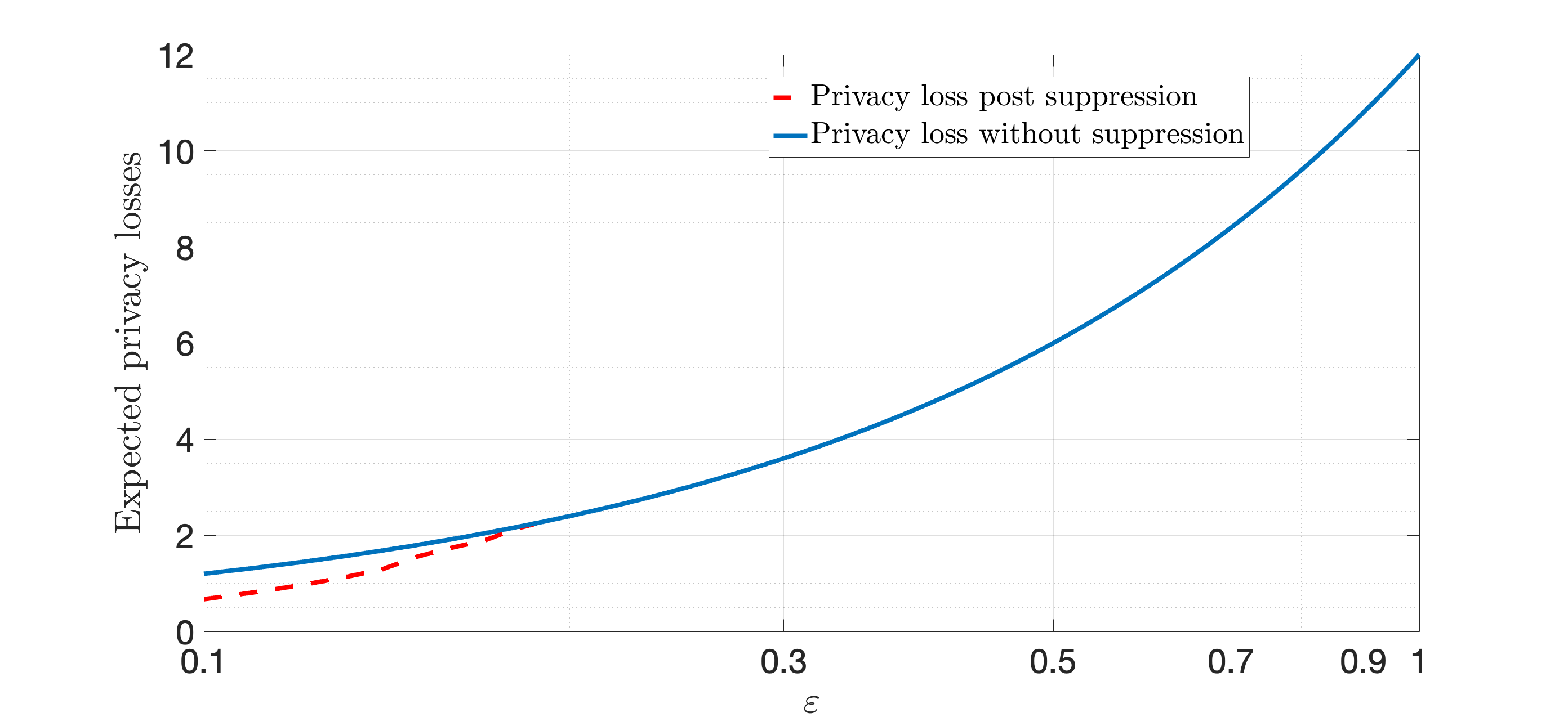
Figure 1. Plot of estimate $\widehat{P}_{\epsilon}$ of expected privacy loss, after execution of Clip-User, against the original privacy loss degradation $G\epsilon$. Here, $\gamma=3$ and $q=0.01$.

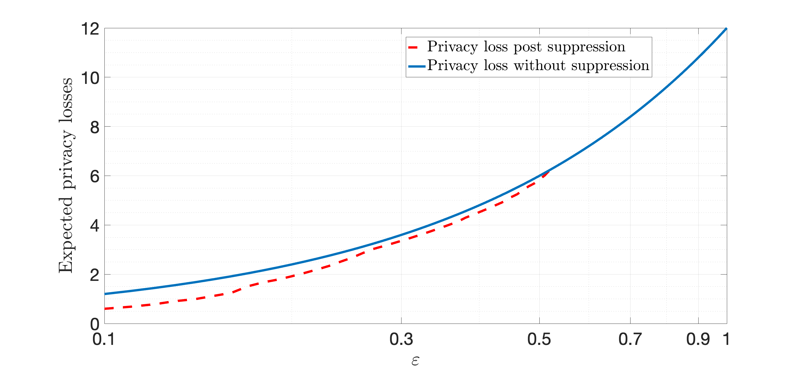
Figure 2. Plot of estimate $\widehat{P}_{\epsilon}$ of expected privacy loss, after execution of Clip-User, against the original privacy loss degradation $G\epsilon$. Here, $\gamma=6$ and $q=0.01$.

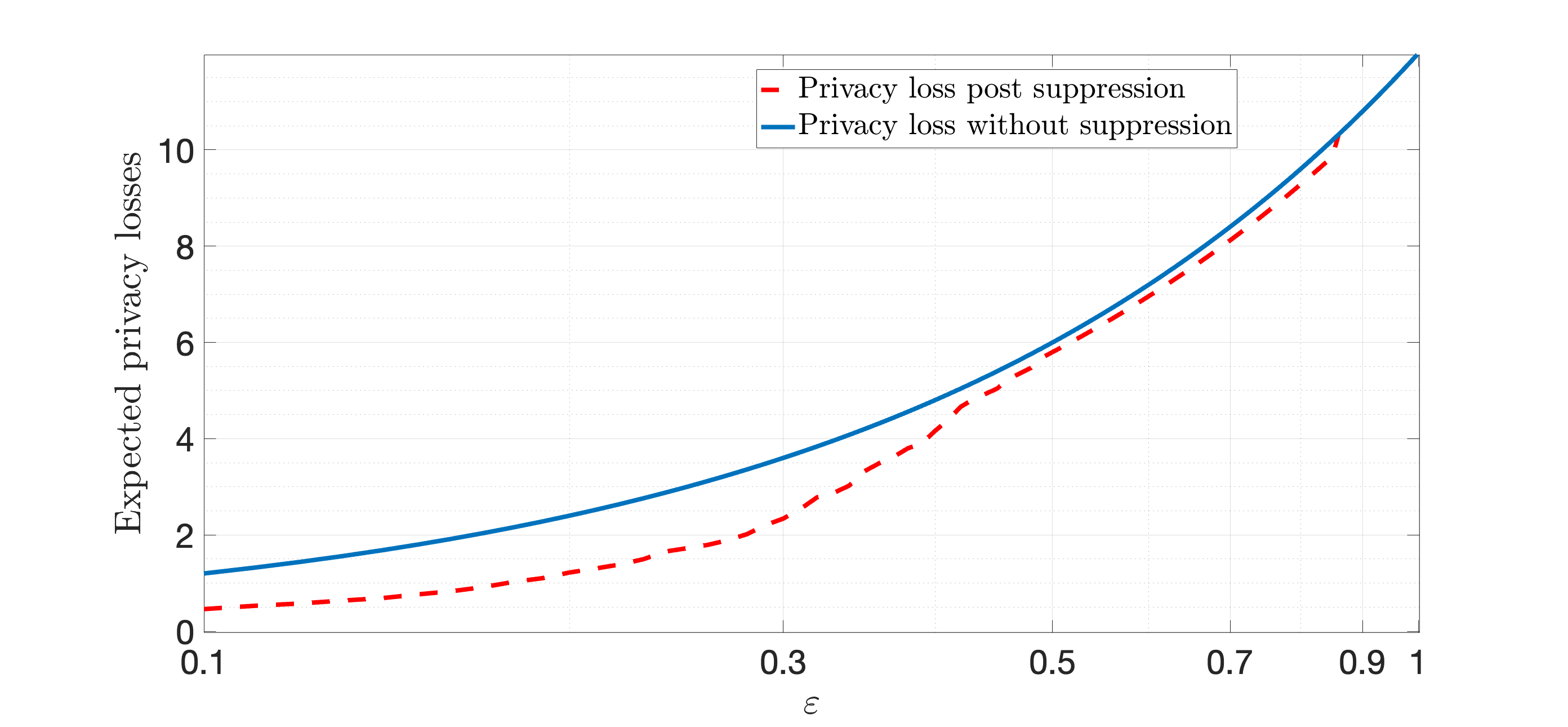
Figure 3. Plot of estimate $\widehat{P}_{\epsilon}$ of expected privacy loss, after execution of Clip-User, against the original privacy loss degradation $G\epsilon$. Here, $\gamma=9$ and $q=0.01$.

Figures 4–6 show plots of the variation of the estimate of the expected worst-case error across grids $\widehat{\overline{E}}_{\epsilon}$ against the original worst-case error $E=E_{\epsilon}$ prior to the execution of Clip-User. Both the $\epsilon$- and the error-axes are shown on a log-scale. Again, it is clear that for a fixed $q\in[0,1]$, increasing $\gamma$ leads to a larger difference between the original and the new worst-case errors, following similar intuition as that earlier.

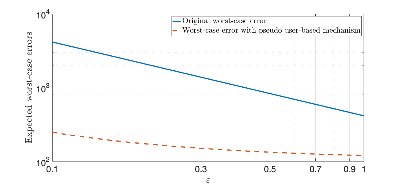
Figure 4. Plot of estimate $\widehat{\overline{E}}_{\epsilon}$ of the worst-case error across grids, after execution of Clip-User and the implementation of the pseudo-user creation-based clipping strategy, against the original worst-case error $E=E_{\epsilon}$. Here, $\gamma=3$ and $q=0.01$.

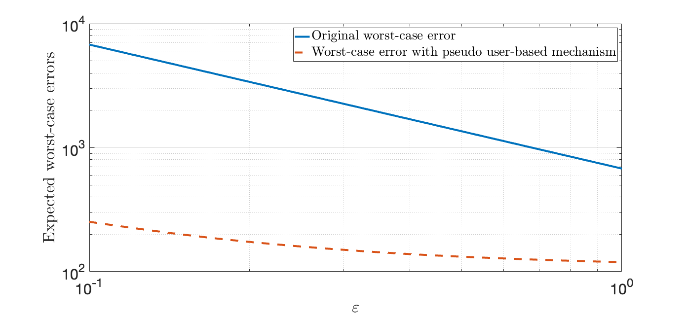
Figure 5. Plot of estimate $\widehat{\overline{E}}_{\epsilon}$ of the worst-case error across grids, after execution of Clip-User and the implementation of the pseudo-user creation-based clipping strategy, against the original worst-case error $E=E_{\epsilon}$. Here, $\gamma=6$ and $q=0.01$.

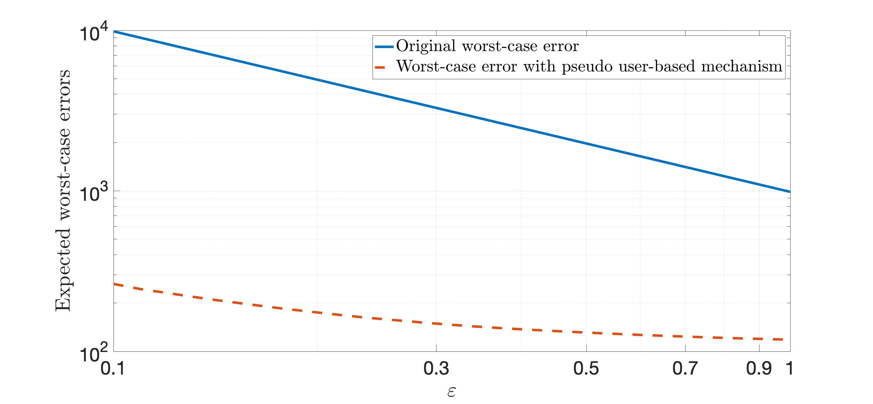
Figure 6. Plot of estimate $\widehat{\overline{E}}_{\epsilon}$ of the worst-case error across grids, after execution of Clip-User and the implementation of the pseudo-user creation-based clipping strategy, against the original worst-case error $E=E_{\epsilon}$. Here, $\gamma=9$ and $q=0.01$.

7. Conclusion

In this paper, we proposed an algorithm for improving the privacy loss degradation under the composition of user-level (pure) differentially private mechanisms that act on disjoint subsets of a dataset, in such a manner as to maintain the worst-case error in estimation over all such subsets. The basic idea behind our algorithm was the clipping of user contributions in selected subsets to improve the privacy loss degradation, while not increasing the worst-case estimation error. In particular, motivated by applications in the release of statistics of traffic data, we considered the design of such an algorithm for the release of the sample mean and variance of speed records in different grids in a city. A key component of the design of our algorithm was the explicit computation of the sensitivity of the sample variance function and the worst-case errors in estimation of the variance due to clipping selected contributions of users. We then presented numerical results evaluating the performance of our algorithm on synthetically generated datasets.

An interesting line of future research would be the extension of the techniques presented in this paper to the private release of other statistics of interest via their counts or histograms.

Appendix A Proof of Proposition 3.1

In this section, we shall prove Proposition 3.1.

Recall from the definition of user-level sensitivity in Section 2 that

$$\Delta_{\textsf{Var}}=\max_{\mathcal{D}\sim\mathcal{D}^{\prime}}\left\lvert\textsf{Var}(\mathcal{D})-\textsf{Var}(\mathcal{D}^{\prime})\right\rvert,$$

where Var is as in (4), and the notation $\mathcal{D}\sim\mathcal{D}^{\prime}$ refers to the fact that $\mathcal{D}$ and $\mathcal{D}^{\prime}$ are user-level neighbours, for $\mathcal{D},\mathcal{D}^{\prime}\in\mathsf{D}$. Moreover, without loss of generality, for the purpose of evaluating $\Delta_{\textsf{Var}}$, we can assume that $\textsf{Var}(\mathcal{D}^{\prime})\leq\textsf{Var}(\mathcal{D})$ in the expression for $\Delta_{\textsf{Var}}$. Now, let

$$\mathsf{D}_{\text{max}}=\left\{(\mathcal{D},\mathcal{D}^{\prime}):(\mathcal{D},\mathcal{D}^{\prime})\in\operatorname*{arg\,max}_{\mathcal{D}\sim\mathcal{D}^{\prime}}\left\lvert\textsf{Var}(\mathcal{D})-\textsf{Var}(\mathcal{D}^{\prime})\right\rvert\right\}$$

be the collection of pairs of neighbouring datasets that attain the maximum in the definition of $\Delta_{\textsf{Var}}$. In what follows, we shall exactly determine $\Delta_{\textsf{Var}}$ by identifying the structure of one pair $(\mathcal{D}_{1},\mathcal{D}_{2})\in\mathsf{D}_{\text{max}}$ of neighbouring datasets.

Suppose that $\mathcal{D}_{1},\mathcal{D}_{2}$ as above differ (exclusively) in the sample values contributed by user $k\in[L]$. Let $\left\{S_{\ell}^{(j)}\right\}$ denote the samples in dataset $\mathcal{D}_{1}$ and $\left\{\tilde{S}_{\ell}^{(j)}\right\}$ denote the samples in dataset $\mathcal{D}_{2}$. Let $\nu$ and $\tilde{\nu}$ be respectively the sample means of $\left\{S_{\ell}^{(j)}\right\}$ and $\left\{\tilde{S}_{\ell}^{(j)}\right\}$. Let ${A}:=\left\{{S}_{k}^{(j)}:\ j\in[m_{k}]\right\}$ and $\tilde{A}:=\left\{\tilde{S}_{k}^{(j)}:\ j\in[m_{k}]\right\}$ be the samples contributed by user $k$ in $\mathcal{D}_{1}$ and $\mathcal{D}_{2}$, respectively. Further, let

$${\nu}(A):=\frac{1}{m_{k}}\cdot\sum_{j=1}^{m_{k}}{S}_{k}^{(j)}\ \ \text{and}\ \ {\nu}(\tilde{A}):=\frac{1}{m_{k}}\cdot\sum_{j=1}^{m_{k}}\tilde{S}_{k}^{(j)}$$

be the means of the samples in $A$ and $\tilde{A}$, respectively. Similarly, let

$${\nu}(A^{c}):=\frac{1}{\sum_{\ell\neq k}m_{\ell}}\cdot\sum_{\ell\neq k}\sum_{j=1}^{m_{\ell}}{S}_{\ell}^{(j)}\ \ \text{and}\ \ {\nu}(\tilde{A}^{c}):=\frac{1}{\sum_{\ell\neq k}m_{\ell}}\cdot\sum_{\ell\neq k}\sum_{j=1}^{m_{\ell}}\tilde{S}_{\ell}^{(j)},$$

where we define $A^{c}$ to be those samples contributed by the users other than user $k$ in $\mathcal{D}_{1}$, and similarly, for $\tilde{A}^{c}$. By the definition of the datasets $\mathcal{D}_{1}$ and $\mathcal{D}_{2}$, we have that $A^{c}=\tilde{A}^{c}$ and hence $\tilde{\nu}(A^{c})=\nu(A^{c})$. Furthermore, the following lemma holds.

Lemma A.0.

There exists $(\mathcal{D}_{1},\mathcal{D}_{2})\in\mathsf{D}_{\text{max}}$ such that

$${\nu}(\tilde{A})={\nu}(A^{c}).$$

Furthermore, we can choose $\tilde{S}_{k}^{(1)}=\ldots=\tilde{S}_{k}^{(m_{k})}={\nu}(\tilde{A})$, in $\mathcal{D}_{2}$.

Proof.

First, we write

$$\Delta_{\textsf{Var}} =\max_{\mathcal{D}\sim\mathcal{D}^{\prime}}\left(\textsf{Var}(\mathcal{D})-\textsf{Var}(\mathcal{D}^{\prime})\right)$$

$$=\max_{\mathcal{D}}\left(\textsf{Var}(\mathcal{D})-\min_{\mathcal{D}^{\prime}\sim\mathcal{D}}\textsf{Var}(\mathcal{D}^{\prime})\right).$$

Now, for a fixed dataset $\mathcal{D}$, consider $\textsf{Var}(\mathcal{D}^{\prime})$, for $\mathcal{D}^{\prime}\sim\mathcal{D}$. Let $\tilde{X}\sim\text{Unif}(\tilde{A}\cup A^{c})$ denote a uniformly distributed random variable that takes values in the set $\left\{\tilde{S}_{\ell}^{(j)}\right\}$. Then,

$$\textsf{Var}(\mathcal{D}^{\prime}) =\mathbb{E}\left[(\tilde{X}-\tilde{\nu})^{2}\right]$$

$$=\mathbb{E}\left[(\tilde{X}-\tilde{\nu})^{2}\mid\tilde{X}\in\tilde{A}\right]\Pr[\tilde{X}\in\tilde{A}]\ +$$

$$\ \ \ \ \ \ \ \ \ \ \ \ \ \ \ \ \mathbb{E}\left[(\tilde{X}-\tilde{\nu})^{2}\mid\tilde{X}\in{A}^{c}\right]\Pr[\tilde{X}\in A^{c}]$$

$$\stackrel{{\scriptstyle(a)}}{{=}}\mathbb{E}\left[(\tilde{X}-\tilde{\nu})^{2}\mid\tilde{X}\in\tilde{A}\right]\cdot\left(\frac{m_{k}}{\sum_{\ell}m_{\ell}}\right)\ +$$

$$\ \ \ \ \ \ \ \ \ \ \ \ \ \ \ \ \mathbb{E}\left[(\tilde{X}-\tilde{\nu})^{2}\mid\tilde{X}\in{A}^{c}\right]\cdot\left(1-\frac{m_{k}}{\sum_{\ell}m_{\ell}}\right)$$

Now, consider the term $\mathbb{E}\left[(\tilde{X}-\tilde{\nu})^{2}\mid\tilde{X}\in\tilde{A}\right]$ above. We can write

$$\mathbb{E}\left[(\tilde{X}-\tilde{\nu})^{2}\mid\tilde{X}\in\tilde{A}\right]$$

$$=\mathbb{E}\left[(\tilde{X}-{\nu}(\tilde{A})+{\nu}(\tilde{A})-\tilde{\nu})^{2}\mid\tilde{X}\in\tilde{A}\right]$$

$$=\mathbb{E}\left[(\tilde{X}-{\nu}(\tilde{A}))^{2}\mid\tilde{X}\in\tilde{A}\right]+(\tilde{\nu}-{\nu}(\tilde{A}))^{2}\ +$$

$$\ \ \ \ \ \ \ \ \ \ \ \ \ \ \ \ \ \ \ \ \ 2\ ({\nu}(\tilde{A})-\tilde{\nu})\cdot\mathbb{E}\left[(\tilde{X}-{\nu}(\tilde{A}))\mid\tilde{X}\in\tilde{A}\right].$$

Clearly, since $\tilde{X}\sim\text{Unif}(\mathcal{D}^{\prime})$, we have that conditioned on the event $\{\tilde{X}\in\tilde{A}\}$, we have that $\tilde{X}$ is uniform on $\tilde{A}$. Therefore, we obtain that $\mathbb{E}\left[(\tilde{X}-{\nu}(\tilde{A}))\mid\tilde{X}\in\tilde{A}\right]=0$, implying that

(15) $$\mathbb{E}\left[(\tilde{X}-\tilde{\nu})^{2}\mid\tilde{X}\in\tilde{A}\right]=\mathbb{E}\left[(\tilde{X}-{\nu}(\tilde{A}))^{2}\mid\tilde{X}\in\tilde{A}\right]+(\tilde{\nu}-{\nu}(\tilde{A}))^{2}.$$

By similar arguments, we obtain that

(16) $$\mathbb{E}\left[(\tilde{X}-\tilde{\nu})^{2}\mid\tilde{X}\in{A}^{c}\right]=\mathbb{E}\left[(\tilde{X}-{\nu}(A^{c}))^{2}\mid\tilde{X}\in{A}^{c}\right]+(\tilde{\nu}-{\nu}({A}^{c}))^{2}.$$

Substituting (15) and (16) into equality (a) above, we get that

$$\textsf{Var}(\mathcal{D}^{\prime})$$

$$=\left(\mathbb{E}\left[(\tilde{X}-{\nu}(\tilde{A}))^{2}\mid\tilde{X}\in\tilde{A}\right]+(\tilde{\nu}-{\nu}(\tilde{A}))^{2}\right)\cdot\left(\frac{m_{k}}{\sum_{\ell}m_{\ell}}\right)\ +$$

$$\ \ \ \ \ \ \ \ \ \ \ \ \left(\mathbb{E}\left[(\tilde{X}-{\nu}(A^{c}))^{2}\mid\tilde{X}\in{A}^{c}\right]+(\tilde{\nu}-{\nu}({A}^{c}))^{2}\right)\cdot\left(1-\frac{m_{k}}{\sum_{\ell}m_{\ell}}\right).$$

Now, observe that all the terms in equality (a) above are non-negative, and hence $\textsf{Var}(\mathcal{D}^{\prime})$ is minimized by setting $\tilde{\nu}={\nu}(\tilde{A})={\nu}({A}^{c})=\tilde{S}_{k}^{(j)}$, for all $j\in[m_{k}]$. ∎

From the proof of the lemma above, we obtain that there exist datasets $(\mathcal{D}_{1}$, $\mathcal{D}_{2})\in\mathsf{D}_{\text{max}}$, such that

$$\textsf{Var}(\mathcal{D}^{\prime})=\mathbb{E}\left[(\tilde{X}-{\nu}(A^{c}))^{2}\mid\tilde{X}\in{A}^{c}\right]\cdot\left(1-\frac{m_{k}}{\sum_{\ell}m_{\ell}}\right).$$

Furthermore, for this choice of $\mathcal{D}_{2}$, we have $\tilde{S}_{k}^{(j)}={\nu}({A}^{c})$, for all $j\in[m_{k}]$. The next lemma provides an alternative characterization of $\Delta_{\textsf{Var}}$, using our choice of datasets $\mathcal{D}_{1}$, $\mathcal{D}_{2}$.

Lemma A.0.

We have that

$$\Delta_{\textsf{Var}} =\max_{\mathcal{D}:\ {S}_{\ell}^{(j)}=\nu(A^{c}),\forall{S}_{\ell}^{(j)}\in A^{c}}\textsf{Var}(\mathcal{D})$$

Proof.

Recall that

$$\Delta_{\textsf{Var}}=\textsf{Var}(\mathcal{D}_{1})-\textsf{Var}(\mathcal{D}_{2}),$$

with $\mathcal{D}_{2}$ chosen as in the discussion preceding this lemma. Thus, for random variables $\tilde{X}\sim\text{Unif}(\tilde{A}\cup A^{c})$ and $X\sim\text{Unif}(A\cup A^{c})$, we have

$$\Delta_{\textsf{Var}}$$

$$=\max_{\mathcal{D}}\left[\textsf{Var}(\mathcal{D})-\mathbb{E}\left[(\tilde{X}-{\nu}(A^{c}))^{2}\mid\tilde{X}\in{A}^{c}\right]\cdot\left(1-\frac{m_{k}}{\sum_{\ell}m_{\ell}}\right)\right]$$

$$=\max_{\mathcal{D}}\left[\mathbb{E}\left[(X-\nu)^{2}\right]-\mathbb{E}\left[(\tilde{X}-{\nu}(A^{c}))^{2}\mid\tilde{X}\in{A}^{c}\right]\cdot\left(1-\frac{m_{k}}{\sum_{\ell}m_{\ell}}\right)\right]$$

$$\stackrel{{\scriptstyle(b)}}{{=}}\max_{\mathcal{D}}\left[\mathbb{E}\left[(X-\nu)^{2}\right]-\mathbb{E}\left[({X}-{\nu}(A^{c}))^{2}\mid{X}\in{A}^{c}\right]\cdot\left(1-\frac{m_{k}}{\sum_{\ell}m_{\ell}}\right)\right],$$

where equality (b) follows from the fact that the distribution of $\tilde{X}$ conditioned on the event $\{\tilde{X}\in A^{c}\}$ is identical to that of $X$ conditioned on the event $\{X\in A^{c}\}$. Hence,

$$\Delta_{\textsf{Var}}$$

$$=\max_{\mathcal{D}}\Bigg{[}\mathbb{E}\left[(X-\nu)^{2}\mid X\in A\right]\Pr[X\in A]$$

$$\ \ \ \ \ \ \ \ \ \ \ \ \ \ \ +\mathbb{E}\left[(X-\nu)^{2}\mid X\in A^{c}\right]\Pr[X\in A^{c}]$$

$$\ \ \ \ \ \ \ \ \ \ \ \ \ \ \ \ \ \ -\mathbb{E}\left[(\tilde{X}-{\nu}(A^{c}))^{2}\mid\tilde{X}\in{A}^{c}\right]\cdot\left(1-\frac{m_{k}}{\sum_{\ell}m_{\ell}}\right)\Bigg{]}.$$

Now, observe that by arguments as in the proof of Lemma A.1,

$$\mathbb{E}\left[(X-\nu)^{2}\mid X\in A^{c}\right] =\mathbb{E}\left[({X}-{\nu}(A^{c}))^{2}\mid{X}\in{A}^{c}\right]+(\nu-\nu(A^{c}))^{2}.$$

Now, since $\Pr[X\in A^{c}]=\left(1-\frac{m_{k}}{\sum_{\ell}m_{\ell}}\right)$, we have by arguments made earlier, that

$$\Delta_{\textsf{Var}} =\max_{\mathcal{D}}\bigg{[}\mathbb{E}\left[(X-\nu)^{2}\mid X\in A\right]\Pr[X\in A]+$$

(17) $$\ \ \ \ \ \ \ \ \ \ \ \ \ \ \ \ \ \ \ \ \ \ \ \ \ \ \ \ \ \ \ \ \ \ (\nu-\nu(A^{c}))^{2}\Pr[X\in A^{c}]\bigg{]}$$

$$=\max_{\mathcal{D}:\ {S}_{\ell}^{(j)}=\nu(A^{c}),\forall{S}_{\ell}^{(j)}\in A^{c}}\textsf{Var}(\mathcal{D}),$$

thereby proving the lemma. ∎

Note that the maximization in the expression in Lemma A.2 is essentially over $\nu(A^{c})$ and the variables $\left\{S_{j}^{(\ell)}\right\}\in A$, with the constraint that ${S}_{\ell}^{(j)}=\nu(A^{c})$, for all ${S}_{\ell}^{(j)}\in A^{c}$. It is easy to show that for a fixed choice of the cariables $\left\{S_{j}^{(\ell)}\right\}\in A$, the expression in (17) is a quadratic function of $\nu(A^{c})$, with a non-negative coefficient. Hence, the maximum over $\nu(A^{c})$ of the expression in (17) is attained at a boundary point, i.e., at either $\nu(A^{c})=0$ or at $\nu(A^{c})=U$. This observation immediately leads to a proof of Proposition 3.1.

Proof of Proposition 3.1.

Recall from Lemma A.2 that

$$\Delta_{\textsf{Var}}=\max_{\mathcal{D}:\ {S}_{\ell}^{(j)}=\nu(A^{c}),\forall{S}_{\ell}^{(j)}\in A^{c}}\textsf{Var}(\mathcal{D}).$$

From the discussion preceding this lemma, consider the case when the maximum over $\nu(A^{c})$ above is attained at $\nu(A^{c})=0$. The proof for the case when $\nu(A^{c})=U$ follows along similar lines, and is hence omitted. In this case,

$$\Delta_{\textsf{Var}}=\max_{{S}_{\ell}^{(j)}\in A:\ {S}_{\ell}^{(j)}=0,\forall{S}_{\ell}^{(j)}\in A^{c}}\textsf{Var}(\mathcal{D}).$$

In this setting, $\nu\leq\frac{Um_{k}}{\sum_{\ell}m_{\ell}}$. Two possible situations arise: (i) when $\sum_{\ell}m_{\ell}>2m^{\star}$, and (ii) when $\sum_{\ell}m_{\ell}\leq 2m^{\star}$. Consider the first situation. In this case, observe that $\nu\leq\frac{Um^{\star}}{\sum_{\ell}m_{\ell}}<U/2$. Further, from the Bhatia-Davis inequality (Bhatia and Davis, 2000), we have $\textsf{Var}(\mathcal{D})\leq\nu(U-\nu)=:b(\nu)$. Hence, for the range of $\nu$ values of interest, we have that $b(\nu)$ is strictly increasing in $\nu$. Hence,

$$\Delta_{\textsf{Var}} \leq\max_{\mathcal{D}:\ {S}_{\ell}^{(j)}=0,\forall{S}_{\ell}^{(j)}\in A^{c}}\nu(U-\nu)$$

$$\leq\frac{U^{2}\ m^{\star}(\sum_{\ell}m_{\ell}-m^{\star})}{\left(\sum_{\ell}m_{\ell}\right)^{2}},$$

with the inequalities above being achieved with equality when $S_{k}^{(j)}=U$, for all $j\in[m_{k}]$, and when $m_{k}=m^{\star}$. Next, consider the situation when $\sum_{\ell}m_{\ell}\geq 2m^{\star}$, and suppose that $\sum_{\ell}m_{\ell}$ is even. In this case, we have that $|A|\geq|A^{c}|$. For this setting, first note that

$$\Delta_{\textsf{Var}}\leq\max_{\mathcal{D}\in\mathsf{D}}\textsf{Var}(\mathcal{D})=\max\textsf{Var}(W)=\frac{U^{2}}{4},$$

for $W\sim\text{Unif}(A\cup A^{c})$. To see why the above bound holds, note that for any bounded random variable $Y\in[0,U]$, we have that

$$\textsf{Var}(Y)=\textsf{Var}(Y-U/2)\leq U^{2}/4.$$

Furthermore, equality above is attained when all samples in $A^{c}$ take the value $0$ (which is in line with the case of interest where $\nu(A^{c})=0$) and $\frac{|A|-|A^{c}|}{2}$ samples in $A$ take the value $0$ and the remaining samples take the value $U$. This then results in exactly $\frac{\sum_{\ell}m_{\ell}}{2}$ samples being $0$ and an equal number of samples being $U$, resulting $\Delta_{\textsf{Var}}=U^{2}/4$.

Next, consider the case when $\sum_{\ell}m_{\ell}$ is odd. In this setting, it is not possible to ensure that equal number of samples (from $A\cup A^{c}$) are at $0$ and $U$, thereby implying that the true value of $\textsf{Var}(\mathcal{D})$, with $S_{j}^{(\ell)}=0$, for all $S_{j}^{(\ell)}\in A^{c}$, in this case is smaller than $U^{2}/4$. We claim that in the case when the total number, $\sum_{\ell}m_{\ell}$, of samples is odd, the variance of a bounded random variable $Y\in[0,U]$ that takes values in $\left\{S_{j}^{(\ell)}\right\}$ obeys

(18) $$\textsf{Var}(Y)\leq\frac{U^{2}}{4}\cdot\left(1-\frac{1}{(\sum_{\ell}m_{\ell})^{2}}\right);$$

furthermore, this bound is achieved when $\left\lceil\frac{\sum_{\ell}m_{\ell}}{2}\right\rceil$ samples take the value $0$ and $\left\lfloor\frac{\sum_{\ell}m_{\ell}}{2}\right\rfloor$ samples take the value $U$. Modulo this claim, observe that in the case where $|A|\geq|A^{c}|$, the upper bound in (18) is achievable when $S_{j}^{(\ell)}=0$, for all $S_{j}^{(\ell)}\in A^{c}$, by placing $\left\lceil\frac{|A|-|A^{c}|}{2}\right\rceil$ samples from $A$ at the value $0$ and the remaining samples at $U$.

We now prove the above claim. To this end, we first show that any sample distribution $\left\{S_{j}^{(\ell)}\right\}$ that maximizes the variance above must be such that $S_{j}^{(\ell)}\in\{0,U\}$, for all $\ell,j$. For ease of reading, we let the samples $\left\{S_{j}^{(\ell)}\right\}$ be written as the collection $\{x_{1},\ldots,x_{n}\}$, where $n=\sum_{\ell}m_{\ell}$. Now, we write

(19) $$\max_{\mathcal{D}}\textsf{Var}(Y)=\max_{x_{1}}\max_{x_{2}}\ldots\max_{x_{n}}\textsf{Var}(Y).$$

Note that for fixed values of $x_{1},x_{2},\ldots,x_{n-1}$, the variance above is maximized when $x_{n}\in\{0,U\}$. To see why, let $\nu_{\sim n}$ denote the sample mean of the samples $x_{1},\ldots,x_{n-1}$ and let $Y_{\sim n}$ denote the random variable that is uniformly distributed over the samples $x_{1},x_{2},\ldots,x_{n-1}$. By arguments as earlier, note that

$$\textsf{Var}(Y)$$

$$=\left(\frac{n-1}{n}\right)\cdot\left(\mathbb{E}\left[(Y-\nu_{\sim n})^{2}\mid Y\neq x_{n}\right]+(\nu-\nu_{\sim n})^{2}\right)+\frac{1}{n}\left(\nu-x_{n}\right)^{2}$$

$$=\left(\frac{n-1}{n}\right)\cdot\textsf{Var}(Y_{\sim n})+\frac{n-1}{n^{2}}\cdot(x_{n}-\nu_{\sim n})^{2}.$$

Clearly, the above expression is maximized, for fixed $x_{1},x_{2},\ldots,x_{n-1}$, by $x_{n}\in\{0,U\}$, depending on the value of $\nu_{\sim n}$. This argument can then be repeated iteratively over all $x_{1},\ldots,x_{n}$, using (19).

Now, since all the samples in the collection $\{x_{1},\ldots,x_{n}\}$ take a value of either $0$ or $U$, all that remains is a maximization of $\textsf{Var}(Y)$, given this constraint. Let $k$ denote the number of samples taking the value $0$ and let $n-k$ be the number of samples taking the value $U$. In this case, $\nu=\frac{(n-k)U}{n}$. Then,

$$\frac{\textsf{Var}(Y)}{U^{2}} =\frac{k}{n}\cdot\left(\frac{n-k}{n}\right)^{2}+\frac{n-k}{n}\cdot\left(\frac{k}{n}\right)^{2}$$

$$=\frac{k(n-k)}{n^{2}}.$$

Clearly, when $n$ is odd, the above expression is maximized when $\left\lceil\frac{n}{2}\right\rceil$ values are $0$ and the remaining $\left\lfloor\frac{n}{2}\right\rfloor$ values are $U$, proving our earlier claim. ∎

Appendix B On the Sensitivities Under a Special Clipping Strategy

In this section, we consider a special class of clipping strategies obtained by setting $\Gamma_{\ell}=\min\{m,m_{\ell}\}$, for some fixed $m\in[m_{\star}:m^{\star}]$. Clearly, here, we have $\Gamma^{\star}=m$ and $\Gamma_{\star}:=\min_{\ell\in\mathcal{L}}\Gamma_{\ell}=m_{\star}$. Such a clipping strategy arises naturally in the design of user-level differentially private mechanisms based on the creation of pseudo-users (George et al., 2022; Arvind Rameshwar et al., 2024). We show that for choices of $m$ of interest, the sensitivities of the clipped sample mean and variance are at most those of their unclipped counterparts. In particular, for the sample mean, the following lemma was shown in (Arvind Rameshwar et al., 2024):

Lemma B.0 (Lemma III.1 in (Arvind Rameshwar et al., 2024)).

For any $m\leq m^{\star}$, we have that $\Delta_{\mu}\geq{\Delta}_{\mu_{\text{clip}}}$.

We now proceed to state and prove an analogous lemma that compares the sensitivities of $\textsf{Var}_{\text{clip}}$ and Var. Before we proceed, observe that it is natural to restrict attention to those values of $m\in[m_{\star}:m^{\star}]$ that minimize the sensitivity of the clipped variance in 3.3. We first show that there exists a minimizer $m\in[m_{\star}:m^{\star}]$ that takes its value in the set $\{m_{\ell}\}_{\ell\in\mathcal{L}}$. Let $\Delta_{\textsf{Var}_{\text{clip}}}(m)=\Delta_{\textsf{Var}_{\text{clip}}}$, for a fixed $m$. To achieve this objective, we need the following helper lemma. For ease of exposition, we assume that $m_{\star}=m_{1}\leq m_{2}\leq\ldots\leq m_{L}=m^{\star}$. We also assume throughout that $L\geq 2$.

Lemma B.0.

$\Delta_{\textsf{Var}_{\text{clip}}}(m)$ is concave in $m$, for $m\in[m_{t},m_{t+1}]$, for any $t\in[L-3]$, when $L\geq 3$.

Proof.

Fix an integer $t\in[L-1]$, for $L\geq 3$. Let $\alpha_{1}(m):=\frac{\Gamma_{\ell}^{\star}(\sum_{\ell}\Gamma_{\ell}-\Gamma_{\ell}^{\star})}{\left(\sum_{\ell}\Gamma_{\ell}\right)^{2}}$, $\alpha_{2}(m):=\frac{1}{4}$, and $\alpha_{3}(m):=\frac{1}{4}\cdot\left(1-\frac{1}{(\sum_{\ell}\Gamma_{\ell})^{2}}\right)$.

Now, consider the setting where $t\leq L-3$. In this case, observe that

$$\sum_{\ell}\Gamma_{\ell} =\sum_{\ell}\min\{m,m_{\ell}\}$$

$$=\sum_{\ell=1}^{t}m_{t}+(L-t)m>2m,$$

by our choice of $t$. This implies that for such values of $t$, we have $\Delta_{\textsf{Var}_{\text{clip}}}(m)=U^{2}\cdot\alpha_{1}(m)$, for all $m\in[m_{t},m_{t+1}]$. Now, observe that we can write

$${\alpha}_{1}(m) =\frac{m(c_{1}+m(c_{2}-1))}{(c_{1}+c_{2}m)^{2}}$$

$$=\frac{m}{c_{1}+c_{2}m}-\frac{m^{2}}{(c_{1}+c_{2}m)^{2}}=:a_{1}(m)+b_{1}(m),$$

for constants $c_{1},c_{2}>0$ such that $c_{1}+c_{2}m=\sum_{\ell}\Gamma_{\ell}$. By direct computation, it is possible to show that

$$\frac{\mathrm{d}^{2}a_{1}}{\mathrm{d}m^{2}}=\frac{-2c_{1}c_{2}}{(c_{1}+c_{2}m)^{3}}<0$$

and

$$\frac{\mathrm{d}^{2}b_{1}}{\mathrm{d}m^{2}}=-2c_{1}\cdot\left(\frac{c_{1}+m(c_{2}-3)}{(c_{1}+c_{2}m)^{4}}\right)\leq 0,$$

since $c_{1}+c_{2}m=\sum_{\ell}\Gamma_{\ell}\geq 3m$, by our choice of $t$. Hence, for this case, we obtain that $\Delta_{\textsf{Var}_{\text{clip}}}(m)$ is concave in $m$. ∎

We are now ready to show that there exists a minimizer of the sensitivity $\Delta_{\textsf{Var}_{\text{clip}}}$ that takes its value in $\{m_{\ell}\}$.

Lemma B.0.

There exists $m\in\operatorname*{arg\,min}_{m\in[m_{\star},m^{\star}]}\Delta_{\textsf{Var}_{\text{clip}}}(m),$ such that $m\in\{m_{\ell}\}_{\ell\in\mathcal{L}}$.

Proof.

Suppose that $m\in[m_{t},m_{t+1}]$, for some $t\in[L-1]$. We now argue that the value of $\Delta_{\textsf{Var}_{\text{clip}}}(m)$ cannot increase by setting $m$ to $\operatorname*{arg\,min}_{m\in\{m_{t},m_{t+1}\}}\Delta_{\textsf{Var}_{\text{clip}}}(m)$. Indeed, note that if $t\in[L-3]$, by the concavity of $\Delta_{\textsf{Var}_{\text{clip}}}(m)$ from Lemma B.2, we obtain that a minimizer of $\Delta_{\textsf{Var}_{\text{clip}}}(m)$, for $m\in[m_{t},m_{t+1}]$, occurs at a boundary point.

Now, consider the case when $t=L-2$. In this case, observe that $\sum\Gamma_{\ell}-2m=\sum_{\ell=1}^{L-2}m_{\ell}>0$, if $L>2$, and equals $0$, if $L\leq 2$. Consider the first case when $L>2$. In this setting, we have $\Delta_{\textsf{Var}_{\text{clip}}}(m)=\alpha_{1}(m)$, for all $m\in[m_{L-2},m_{L-1}]$. It is possible, by direct calculations, to show that when $m\in[m_{L-2},m_{L-1}]$, we have

$$\frac{\mathrm{d}\alpha_{1}}{\mathrm{d}m}=\frac{-2mc_{1}}{(c_{1}+c_{2}m)^{3}},$$

for some constants $c_{1},c_{2}>0$, thereby implying that $\alpha_{1}$ is decreasing as a function of $m$, in this interval. Therefore, a minimizer of $\Delta_{\textsf{Var}_{\text{clip}}}$ occurs at a boundary point.

Next, consider the case when $L=2$. In this setting, we have that $\Delta_{\textsf{Var}_{\text{clip}}}(m)$ equals either $\alpha_{2}(m)$ or $\alpha_{3}(m)$, for $m\in[m_{L-2},m_{L-1}]$, when $\sum_{\ell}\Gamma_{\ell}$ is even or odd, respectively. Since $\alpha_{2}(m)$ is a constant and $\alpha_{3}(m)$ can be seen to be increasing in $m$ in this interval, we obtain once again that a minimizer of $\Delta_{\textsf{Var}_{\text{clip}}}$ occurs at a boundary point.

Now, consider the case when $t=L-1$. Observe that in this case, $\sum_{\ell}\Gamma_{\ell}-2m=\sum_{\ell=1}^{L-1}m_{\ell}-m$ is decreasing as $m$ increases from $m_{L-1}$ to $m_{L}$. Hence, one of three possible cases can occur, each of which is dealt with in turn, below.

1. $\sum_{\ell}\Gamma_{\ell}\leq 2m$, for all $m\in[m_{L-1},m_{L}]$: Clearly, in this case, we have that $\Delta_{\textsf{Var}_{\text{clip}}}$ equals either $\alpha_{2}$ or $\alpha_{3}$, for $m\in[m_{L-2},m_{L-1}]$, when $\sum_{\ell}\Gamma_{\ell}$ is even or odd, respectively. Since $\alpha_{2}$ is a constant and $\alpha_{3}(m)$ is increasing with $m$ in the interval of interest, we obtain that a minimizer of $\Delta_{\textsf{Var}_{\text{clip}}}$ occurs at a boundary point.

2. $\sum_{\ell}\Gamma_{\ell}>2m$, for all $m\in[m_{L-1},m_{L}]$: Here, $\Delta_{\textsf{Var}_{\text{clip}}}=\alpha_{1}$. Furthermore, we have that

   $$\frac{\mathrm{d}\alpha_{1}}{\mathrm{d}m}=\frac{\sum_{\ell=1}^{L-1}m_{\ell}}{(m+\sum_{\ell=1}^{L-1}m_{\ell})^{2}}>0,$$

   implying that $\Delta_{\textsf{Var}_{\text{clip}}}$ is increasing in the interval of interest, hence showing that its minimizer occurs at a boundary point.

3. $\sum_{\ell}\Gamma_{\ell}>2m$, for $m\in[m_{L-1},\overline{m}]$ and $\sum_{\ell}\Gamma_{\ell}\leq 2m$, for $m\in(\overline{m},m_{L}]$, for some $\overline{m}\in[m_{L-1},m_{L}]$: Observe first that in this setting, we have that when $m=\overline{m}$,

   $$\sum_{\ell}\Gamma_{\ell}=\overline{m}+\sum_{\ell=1}^{L-1}m_{\ell}=2\overline{m},$$

   by the definition of $\overline{m}$. In other words, we have $\overline{m}=\sum_{\ell=1}^{L-1}m_{\ell}$. Furthermore, for $m\in[m_{L-1},\overline{m}]$, we have $\Delta_{\textsf{Var}_{\text{clip}}}(m)=\alpha_{1}(m)$, while for $m\in(\overline{m},m_{L}]$, we have $\Delta_{\textsf{Var}_{\text{clip}}}(m)$ equals $\alpha_{2}(m)$ or $\alpha_{3}(m)$, respectively, depending on whether $\sum_{\ell}\Gamma_{\ell}$ is even or odd. In the case when $\sum_{\ell}\Gamma_{\ell}$ is even, it can be verified that $\Delta_{\textsf{Var}_{\text{clip}}}(\overline{m})=\alpha_{2}(m)=1/4$. Thus, using the fact that $\alpha_{1}(m)$ is increasing in $m$, we obtain that a minimizer of $\Delta_{\textsf{Var}_{\text{clip}}}$ occurs at a boundary point, when $\sum_{\ell}\Gamma_{\ell}$ is even.

   Next, when $\sum_{\ell}\Gamma_{\ell}$ is odd, we have that $\alpha_{3}(m)$ is increasing in $m$ for the interval of interest; we thus need only verify if for $L\geq 2$, we have

   $$\alpha_{3}(\overline{m})\geq\alpha_{1}(m_{L-1}).$$

   Indeed, if the above inequality holds, we have that $\Delta_{\textsf{Var}_{\text{clip}}}(\overline{m})$ is minimized at $m=m_{L-1}$, for $m\in[m_{L-1},m_{L}]$. We can verify that the above inequality indeed holds, by a simple direct computation.

Hence, overall, we have that a minimizer of $\Delta_{\textsf{Var}_{\text{clip}}}({m})$, for $m\in[m_{t},m_{t+1}]$ occurs at a boundary point, for all $t\in[L-1]$. ∎

Now that we have established that it suffices to focus on $m\in\{m_{\ell}\}_{\ell\in\mathcal{L}}$, we show that $\Delta_{\textsf{Var}_{\text{clip}}}(m)$, for such values of $m$, is smaller than $\Delta_{\textsf{Var}}$.

Lemma B.0.

When $\sum_{\ell}m_{\ell}$ is even, for $m\in\{m_{\ell}\}_{\ell\in\mathcal{L}}$, we have that $\Delta_{\textsf{Var}}\geq\Delta_{\textsf{Var}_{\text{clip}}}$.

Proof.

The proof proceeds by a case-by-case analysis. First, observe that if $m=m^{\star}$, we have that $\Gamma_{\ell}=m_{\ell}$, for all $\ell\in\mathcal{L}$, implying that $\Delta_{\textsf{Var}}=\Delta_{\textsf{Var}_{\text{clip}}}$. Hence, in what follows, we restrict attention to the case when $m\in[m_{\star}:m^{\star}-1]$. Four possible scenarios arise:

1. $\sum_{\ell}m_{\ell}\leq 2m$: In this case, note that

   $$\sum_{\ell}\Gamma_{\ell}<\sum_{\ell}m_{\ell}\leq 2m<2m^{\star}.$$

   Hence, we have that $\Delta_{\textsf{Var}}=U^{2}/4$, with $\Delta_{\textsf{Var}_{\text{clip}}}=U^{2}/4$, if $\sum_{\ell}\Gamma_{\ell}$ is even, and $\Delta_{\textsf{Var}_{\text{clip}}}=\frac{U^{2}}{4}\cdot\left(1-\frac{1}{(\sum_{\ell}\Gamma_{\ell})^{2}}\right)$, if $\sum_{\ell}\Gamma_{\ell}$ is odd. Clearly, the statement of the lemma is true in this case.

2. $\sum_{\ell}\Gamma_{\ell}\leq 2m\leq\sum_{\ell}m_{\ell}\leq 2m^{\star}$: Here too, $\Delta_{\textsf{Var}}=U^{2}/4$, with $\Delta_{\textsf{Var}_{\text{clip}}}=U^{2}/4$, if $\sum_{\ell}\Gamma_{\ell}$ is even, and $\Delta_{\textsf{Var}_{\text{clip}}}=\frac{U^{2}}{4}\cdot\left(1-\frac{1}{(\sum_{\ell}\Gamma_{\ell})^{2}}\right)$, if $\sum_{\ell}\Gamma_{\ell}$ is odd. The lemma thus holds in this case as well.

3. $2m<\sum_{\ell}\Gamma_{\ell}$: In this case, observe that

   $$2m<\sum_{\ell}\Gamma_{\ell}<\sum_{\ell}m_{\ell}.$$

   Hence, we have that $\Delta_{\textsf{Var}_{\text{clip}}}=\frac{U^{2}\ m(\sum_{\ell}\Gamma_{\ell}-m)}{\left(\sum_{\ell}\Gamma_{\ell}\right)^{2}}$. First, consider the case where $\sum_{\ell}m_{\ell}>2m^{\star}$.

   Again, without loss of generality, assume that $m_{1}\geq m_{2}\geq\ldots\geq m_{L}$. Let us define $\eta(t):=\frac{U^{2}\ m^{\star}(t-m^{\star})}{t^{2}}$, where $t\in(0,\infty)$. It is easy to show that $\frac{\mathrm{d}\eta}{\mathrm{d}t}<0$, implying that $\eta(t)$ is decreasing in its argument $t$. Furthermore, if $m=m_{1}=m^{\star}$, it is easy to see that $\Delta_{\textsf{Var}_{\text{clip}}}=\Delta_{\textsf{Var}}$. Now, suppose that $m=m_{j+1}$, for some $j\in[L-1]$, such that $m<m^{\star}=m_{1}$. Then, since $\sum_{\ell}m_{\ell}<(j+1)m_{1}+\sum_{\ell=j+2}^{L}m_{\ell}=:c$, we have by the above analysis of the function $\eta$ that

   $$\Delta_{\textsf{Var}}>\frac{U^{2}m^{\star}((j+1)m_{1}+c-m^{\star})}{((j+1)m_{1}+c)^{2}}=:\alpha$$

   We next show that $\alpha\geq\Delta_{\textsf{Var}_{\text{clip}}}(m)$. To this end, observe that

   $$\Delta_{\textsf{Var}_{\text{clip}}}=\frac{U^{2}m((j+1)m+c-m)}{((j+1)m+c)^{2}}.$$

   The result follows by explicitly computing $\alpha-\Delta_{\textsf{Var}_{\text{clip}}}$ and arguing that this difference is non-negative, so long as $j\geq 2$, and hence, in particular, when $m<m^{\star}$. Hence, when $\frac{m_{\star}}{m^{\star}}>\frac{2}{L}$ and $m\in\{m_{\ell}\}$, we have that $\Delta_{\textsf{Var}_{\text{clip}}}<\Delta_{\textsf{Var}}$. For $\sum_{\ell}m_{\ell}\leq 2m^{\star}$, we have that $\Delta_{\textsf{Var}}=U^{2}/4\geq\Delta_{\textsf{Var}_{\text{clip}}}$, by a direct calculation.

4. $\sum_{\ell}\Gamma_{\ell}\leq 2m<2m^{\star}\leq\sum_{\ell}m_{\ell}$: We claim that such a situation cannot arise, for the given choice of $\Gamma_{\ell}$, $\ell\in\mathcal{L}$. Indeed, observe that for $m\neq m^{\star}$, for $\sum_{\ell}\Gamma_{\ell}=\sum_{\ell}\min\{m,m_{\ell}\}\leq 2m$ to hold, we must have that for some $\ell_{0}\in\mathcal{L}$, the inequality $m_{\ell_{0}}>m$ holds, while $\sum_{\ell\neq\ell_{0}}m_{\ell}\leq m$. This then implies that

   $$\sum_{\ell}m_{\ell} =m_{\ell_{0}}+\sum_{\ell\neq\ell_{0}}m_{\ell}\leq m$$

   $$<m+m^{\star}<2m^{\star}.$$

   However, by assumption, we have that $2m^{\star}\leq\sum_{\ell}m_{\ell}$, leading to a contradiction.

Putting together all the cases concludes the proof of the lemma. ∎

Appendix C Proof of Theorem 4.2

In this section, we shall prove Theorem 4.2. Recall that we intend computing

$$E_{\textsf{Var}}:=\max_{\mathcal{D}\in\mathsf{D}}\lvert\textsf{Var}(\mathcal{D})-\textsf{Var}_{\text{clip}}(\mathcal{D})\rvert,$$

for fixed $\Gamma_{\ell}\in[0:m_{\ell}]$, for $\ell\in\mathcal{L}$, with the assumption that $\sum_{\ell}\Gamma_{\ell}>0$. For the case when $\Gamma_{\ell}=m_{\ell}$, for all $\ell\in\mathcal{L}$, it is clear that $\textsf{Var}(\mathcal{D})=\textsf{Var}_{\text{clip}}(\mathcal{D})$ and hence that $E_{\textsf{Var}}=0$. Hence, in what follows, we assume that there exists at least one user $\ell\in\mathcal{L}$ with $\Gamma_{\ell}<m_{\ell}$. Let $A:=\left\{S_{\ell}^{(j)}:\ \ell\in\mathcal{L},\ j\in[\Gamma_{\ell}]\right\}$, and define

$$A^{c}:=\left\{S_{\ell}^{(j)}:\ \ell\in\mathcal{L},\ j\in[\Gamma_{\ell}+1:m_{\ell}]\right\}.$$

Now, two cases can possibly arise: (i) when $|A|\leq|A^{c}|$, and (ii) when $|A|>|A^{c}|$. Consider first case (i). Similar to the arguments made in the proof of Proposition 3.1, when $\sum_{\ell}m_{\ell}$ is even, we have that

$$E_{\textsf{Var}}\leq\max_{\mathcal{D}\in\mathsf{D}}\textsf{Var}(\mathcal{D})=\max\textsf{Var}(X)=\frac{U^{2}}{4},$$

for $X\sim\text{Unif}(A\cup A^{c})$. Furthermore, equality above is attained when all samples in $A$ take the value $0$, and $\frac{|A^{c}|-|A|}{2}$ samples in $A^{c}$ take the value $0$ and the remaining samples take the value $U$. This then results in exactly $\frac{\sum_{\ell}m_{\ell}}{2}$ samples being $0$ and an equal number of samples being $U$, resulting in a variance of $U^{2}/4$. Further, when $\sum_{\ell}m_{\ell}$ is odd, we have that

$$E_{\textsf{Var}}\leq\max_{\mathcal{D}\in\mathsf{D}}\textsf{Var}(\mathcal{D})=\max\textsf{Var}(X)=\frac{U^{2}}{4}\cdot\left(1-\frac{1}{(\sum_{\ell}m_{\ell})^{2}}\right),$$

with equality achieved when exactly $\left\lceil\frac{\sum_{\ell}m_{\ell}}{2}\right\rceil$ samples are $0$ and $\left\lfloor\frac{\sum_{\ell}m_{\ell}}{2}\right\rfloor$ samples are $U$. This then gives rise to an exact characterization of $E_{\textsf{Var}}$ when $\sum_{\ell}\Gamma_{\ell}\leq\frac{\sum_{\ell}m_{\ell}}{2}$.

The setting of case (ii), when $|A|>|A^{c}|$, requires more work. However, the proof in this case is quite similar to the proof of Proposition 3.1. As in Appendix A, we define

$${\mu}(A):=\frac{1}{\sum_{\ell}\Gamma_{\ell}}\cdot\sum_{\ell\in\mathcal{L}}\sum_{j=1}^{\Gamma_{\ell}}{S}_{\ell}^{(j)}$$

and

$${\mu}({A}^{c}):=\frac{1}{\sum_{\ell}(m_{\ell}-\Gamma_{\ell})}\cdot\sum_{\ell\in\mathcal{L}}\sum_{j=\Gamma_{\ell}+1}^{m_{\ell}}{S}_{\ell}^{(j)}$$

as the sample means of the samples in the sets $A$ and $A^{c}$, respectively. Further, let $\mu=\mu(\mathcal{D})$. The following lemma then holds.

Lemma C.0.

When $|A|>|A^{c}|$, we have that

$$E_{\textsf{Var}}=\max_{\mathcal{D}\in\mathsf{D}}\left(\textsf{Var}(\mathcal{D})-\textsf{Var}_{\text{clip}}(\mathcal{D})\right).$$

Proof.

(20) $$\textsf{Var}(\mathcal{D})$$

$$=\mathbb{E}_{X\sim\text{Unif}(A\cup A^{c})}\left[(X-\mu)^{2}\right]$$

$$=\mathbb{E}\left[(X-\mu)^{2}\mid X\in A\right]\cdot\mathbb{P}(A)+\mathbb{E}\left[(X-\mu)^{2}\mid X\in A^{c}\right]\cdot P(A^{c})$$

$$=(\mu-\mu(A))^{2}\cdot P(A)+\mathbb{E}\left[(X-\mu(A))^{2}\mid X\in A\right]\cdot P(A)+$$

(21) $$\ \ \ \ \ \ \ \ \ \ \ (\mu-\mu(A^{c}))^{2}\cdot P(A^{c})+\mathbb{E}\left[(X-\mu(A^{c}))^{2}\mid X\in A^{c}\right]\cdot P(A^{c}),$$

where we abbreviate $\Pr[X\in T]$ as $P(T)$, for some set $T\subseteq A\cup A^{c}$. The last equality holds for reasons similar to those in (15) and (16).

Next, note that

(22) $$\textsf{Var}_{\text{clip}}(\mathcal{D})$$

$$=\mathbb{E}_{X^{\prime}\sim\text{Unif}(A)}\left[(X^{\prime}-\mu(A))^{2}\right]$$

(23) $$=\mathbb{E}\left[(X-\mu(A))^{2}\mid X\in A\right]P(A)+\mathbb{E}\left[(X-\mu(A))^{2}\mid X\in A\right]P(A^{c}).$$

Putting together (21) and (23) and noting that, conditioned on the event $\{X\in A\}$, we have that $X$ is uniform on the values in the set $A$, we get that

$$\lvert\textsf{Var}(\mathcal{D})-\textsf{Var}_{\text{clip}}(\mathcal{D})\rvert=$$

$$\bigg{|}(\mu-\mu(A))^{2}P(A)+(\mu-\mu(A^{c}))^{2}P(A^{c})\ +$$

(24) $$\mathbb{E}\left[(X-\mu(A^{c}))^{2}\mid X\in A^{c}\right]P(A^{c})-E\left[(X-\mu(A))^{2}\mid X\in A\right]P(A^{c})\bigg{|}$$

Now, consider a dataset $\overline{\mathcal{D}}$ such that the samples in $A$ take the value $0$ and the samples in $A^{c}$ take the value $U$. Clearly, we have that

(25) $$E_{\textsf{Var}} \geq E_{\textsf{Var}}(\overline{\mathcal{D}})=\frac{U^{2}\cdot|A|\cdot|A^{c}|}{\left(\sum_{\ell}m_{\ell}\right)^{2}}$$

Furthermore, observe that

$$E_{\textsf{Var}}$$

(26) $$=\max\left\{\max_{\mathcal{D}}\left(\textsf{Var}(\mathcal{D})-\textsf{Var}_{\text{clip}}(\mathcal{D})\right),\max_{\mathcal{D}}\left(\textsf{Var}_{\text{clip}}(\mathcal{D})-\textsf{Var}(\mathcal{D})\right)\right\}.$$

Now, from (24), note that

$$\max_{\mathcal{D}}\left(\textsf{Var}_{\text{clip}}(\mathcal{D})-\textsf{Var}(\mathcal{D})\right) \leq\mathbb{E}\left[(X-\mu(A))^{2}\mid X\in A\right]P(A^{c})$$

(27) $$\leq\frac{U^{2}|A^{c}|}{4\cdot\sum_{\ell}m_{\ell}}$$

By comparing (25) and (27), plugging back into (26), and noting that $|A|>|A^{c}|$, we obtain the statement of the lemma. ∎

Thus, from the above lemma and from (24), we obtain that when $|A|>|A^{c}|$,

$$E_{\textsf{Var}}=(\mu-\mu(A))^{2}P(A)+(\mu-\mu(A^{c}))^{2}P(A^{c})\ +$$

$$\mathbb{E}\left[(X-\mu(A^{c}))^{2}\mid X\in A^{c}\right]P(A^{c})-E\left[(X-\mu(A))^{2}\mid X\in A\right]P(A^{c}).$$

Now, clearly, we have that $E_{\textsf{Var}}$ above is maximized by setting $X=\mu(A)$, when $X\in A$, or, in other words, setting $S_{\ell}^{(j)}=\mu(A)$, for all $\ell\in\mathcal{L}$ and $j\in[\Gamma_{\ell}]$. We thus obtain the following lemma:

Lemma C.0.

When $|A|>|A^{c}|$, we have that

$$E_{\textsf{Var}}=\max_{\mathcal{D}:\ S_{\ell}^{(j)}=\mu(A),\forall S_{\ell}^{(j)}\in A}\textsf{Var}(\mathcal{D}).$$

Note the similarity between Lemma C.2 and Lemma A.2 in Appendix A. The proof of Theorem 4.2 is then immediate.

Proof of Theorem 4.2.

Following on from Lemma C.2, by arguments analogous to those in the proof of Proposition 3.1 in Appendix A, we get that when $|A|>|A^{c}|$, $E_{\textsf{Var}}=\frac{U^{2}\cdot|A|\cdot|A^{c}|}{\left(\sum_{\ell}m_{\ell}\right)^{2}}$, which in turn equals $\frac{U^{2}\cdot\sum_{\ell}\Gamma_{\ell}\cdot\sum_{\ell^{\prime}}(m_{\ell^{\prime}}-\Gamma_{\ell^{\prime}})}{\left(\sum_{\ell}m_{\ell}\right)^{2}}$. The case when $|A|\leq|A^{c}|$ was already discussed earlier, wherein $E_{\textsf{Var}}=\frac{U^{2}}{4}$, if $\sum_{\ell}m_{\ell}$ is even, and $E_{\textsf{Var}}=\frac{U^{2}}{4}\cdot\left(1-\frac{1}{(\sum_{\ell}m_{\ell})^{2}}\right)$, if $\sum_{\ell}m_{\ell}$ is odd. ∎

References

• (1)
• h3 ( Inc) Uber Technologies Inc.. H3: Hexagonal hierarchical geospatial indexing system. https://h3geo.org/
• Arvind Rameshwar et al. (2024) V. Arvind Rameshwar, Anshoo Tandon, Prajjwal Gupta, Novoneel Chakraborty, and Abhay Sharma. 2024. Mean Estimation with User-Level Privacy for Spatio-Temporal IoT Datasets. arXiv e-prints, Article arXiv:2401.15906 (Jan. 2024), arXiv:2401.15906 pages. https://doi.org/10.48550/arXiv.2401.15906 arXiv:2401.15906 [cs.CR]
• Bhatia and Davis (2000) Rajendra Bhatia and Chandler Davis. 2000. A Better Bound on the Variance. The American Mathematical Monthly 107, 4 (2000), 353–357. https://doi.org/10.1080/00029890.2000.12005203 arXiv:https://doi.org/10.1080/00029890.2000.12005203
• Dwork et al. (2006) Cynthia Dwork, Frank McSherry, Kobbi Nissim, and Adam Smith. 2006. Calibrating noise to sensitivity in private data analysis. Theory of Cryptography (2006), 265–284. https://doi.org/10.1007/11681878_14
• Dwork and Roth (2014) Cynthia Dwork and Aaron Roth. 2014. The Algorithmic Foundations of Differential Privacy. Foundations and Trends® in Theoretical Computer Science 9, 3–4 (2014), 211–407. https://doi.org/10.1561/0400000042
• Dwork et al. (2010) Cynthia Dwork, Guy N. Rothblum, and Salil Vadhan. 2010. Boosting and Differential Privacy. In 2010 IEEE 51st Annual Symposium on Foundations of Computer Science. 51–60. https://doi.org/10.1109/FOCS.2010.12
• Geng et al. (2015) Quan Geng, Peter Kairouz, Sewoong Oh, and Pramod Viswanath. 2015. The Staircase Mechanism in Differential Privacy. IEEE Journal of Selected Topics in Signal Processing 9, 7 (2015), 1176–1184. https://doi.org/10.1109/JSTSP.2015.2425831
• Geng and Viswanath (2014) Quan Geng and Pramod Viswanath. 2014. The optimal mechanism in differential privacy. In 2014 IEEE International Symposium on Information Theory. 2371–2375. https://doi.org/10.1109/ISIT.2014.6875258
• George et al. (2022) Anand Jerry George, Lekshmi Ramesh, Aditya Vikram Singh, and Himanshu Tyagi. 2022. Continual Mean Estimation Under User-Level Privacy. arXiv e-prints, Article arXiv:2212.09980 (Dec. 2022), arXiv:2212.09980 pages. https://doi.org/10.48550/arXiv.2212.09980 arXiv:2212.09980 [cs.LG]
• Kairouz et al. (2017) Peter Kairouz, Sewoong Oh, and Pramod Viswanath. 2017. The Composition Theorem for Differential Privacy. IEEE Transactions on Information Theory 63, 6 (2017), 4037–4049. https://doi.org/10.1109/TIT.2017.2685505
• Kamath and Ullman (2020) Gautam Kamath and Jonathan Ullman. 2020. A primer on private statistics. arXiv e-prints, Article arXiv:2005.00010 (April 2020), arXiv:2005.00010 pages. https://doi.org/10.48550/arXiv.2005.00010 arXiv:2005.00010 [stat.ML]
• Levy et al. (2021) Daniel Asher Nathan Levy, Ziteng Sun, Kareem Amin, Satyen Kale, Alex Kulesza, Mehryar Mohri, and Ananda Theertha Suresh. 2021. Learning with User-Level Privacy. In Advances in Neural Information Processing Systems, A. Beygelzimer, Y. Dauphin, P. Liang, and J. Wortman Vaughan (Eds.). https://openreview.net/forum?id=G1jmxFOtY_
• Narayanan and Shmatikov (2008) Arvind Narayanan and Vitaly Shmatikov. 2008. Robust De-anonymization of Large Sparse Datasets. In 2008 IEEE Symposium on Security and Privacy (sp 2008). 111–125. https://doi.org/10.1109/SP.2008.33
• Pandurangan (2014) V. Pandurangan. 2014. On Taxis and Rainbow Tables: Lessons for researchers and governments from NYC’s improperly anonymized taxi logs. https://blogs.lse.ac.uk/impactofsocialsciences/2014/07/16/nyc-improperly-anonymized-taxi-logs-pandurangan/
• Steinke (2022) Thomas Steinke. 2022. Composition of Differential Privacy & Privacy Amplification by Subsampling. arXiv e-prints, Article arXiv:2210.00597 (Oct. 2022), arXiv:2210.00597 pages. https://doi.org/10.48550/arXiv.2210.00597 arXiv:2210.00597 [cs.CR]
• Sweeney (1997) Latanya Sweeney. 1997. Weaving technology and policy together to maintain confidentiality. Journal of Law, Medicine & Ethics 25, 2–3 (1997), 98–110. https://doi.org/10.1111/j.1748-720x.1997.tb01885.x
• Vadhan (2017) Salil Vadhan. 2017. The Complexity of Differential Privacy. Springer, Yehuda Lindell, ed., 347–450. https://link.springer.com/chapter/10.1007/978-3-319-57048-8_7
• Whong (2014) C. Whong. 2014. FOILing NYC’s Taxi Trip Data. https://chriswhong.com/open-data/foil_nyc_taxi/