Designing a polymerized phenalenyl tessellation molecule to realize a super-honeycomb antiferromagnetic $S=3/2$ spin system

Abstract

In a multiply hydrogenated polymer of phenalenyl tessellation molecules (PTMs) where spatially overlapping zero modes appear, three parallelly spin-aligned electron spins per PTM are generated by the direct exchange interaction of the strongly correlated electron system, which we used to facilitate the molecular design of a two-dimensional (2D) $S=3/2$ Heisenberg spin system on a honeycomb lattice. Density functional theory with the Wannierization method simulations of the electronic structure suggested that an array of nonbonding molecular orbitals (an array of zero modes) appears in the hydrogenated nanographene structure. Our evaluation of the onsite interaction strength indicated that each zero mode becomes half-filled with a spin-active electron by the electron correlation effect. The low-energy subspace of the obtained zero mode-tight-binding model implies the appearance of a 2D antiferromagnetic $S=3/2$ Heisenberg system with the entangled quantum spin ground state.

1 Introduction

The proposal of measurement-based quantum computation[1, 2] increased interest in realizing resource states in a realistic system.[3, 4] This led to the hope that hardware systems should possess or produce quantum entangled states, which are classified as topological cluster states in optical lattices[5, 6] and/or the spin-3/2 Affleck–Kennedy–Lieb–Tasaki (AKLT) state in a spin system.[7, 8] For the former system, implementation is a problem because the measurement of an individual atom qubit is not easy. For the latter system, a designed alignment of quantum spins has to be realized.[9] There have been several attempts to realize quantum spin-1 systems[10, 11] and a spin-1/2 system on a star lattice[12] using carbon-based materials such as nanographene. In these studies, a major design principle is the nonbonding molecular orbital (NBMO). The disjoint NBMO method involves creating NBMOs and connecting them in a disjointed manner, which leaves the NBMOs as eigenstates of a hopping Hamiltonian.[13, 14, 15, 16]

In a spin system, a qubit is expected to have a nuclear or electron spin. The strength and controllability of inter-spin interaction has to be properly given to facilitate a measurable quantum oscillation. Although electron spins often suffer from environments causing decoherence, we considered an electron spin system appearing in an isolated hydrocarbon molecule owing to the availability of many strategies for designing magnetic spin systems. Such a system should possess some flexibility in its structure and stability in its ideal isolated realization. Material design requires a method that can generate strong magnetic interactions, which cannot be obtained solely by the disjoint NBMO method. In addition, the material should be designed with a strong correlation limit to exhibit stable local spin moments at $S>1/2$.

We considered hydrocarbon materials because each molecule can act as a 2D $S=3/2$ spin system. Molecular design by means of polymerized phenalenyl tessellation makes it possible to draw desirable connections among $\pi$ electron orbitals.[17] A relevant strategy is the design of zero modes, which are NBMOs with topological origins. The generation of $S=3/2$ spins is caused by the appearance of three zero modes that spatially overlap and are spin-aligned by ferromagnetic direct exchange interactions.

To guarantee the feasibility of the material solutions, we utilized a renormalization approach. Density functional theory (DFT) simulations[18, 19] and the Wannierization method[20] were used to evaluate the structures of the hydrocarbon materials and confirm their stability. A low-energy effective model was derived by the Wannierization method, and the estimation of the effective inter-electron interaction indicated the development of an antiferromagnetic $S=3/2$ spin system.

2 Molecular design and confirmation methods

2.1 $\pi$-network design

The phenalenyl molecule is a polycyclic alternant hydrocarbon made of three benzene rings. To design hydrocarbon systems with appropriately arranged zero modes, we selected the method of generating a polymerized phenalenyl-tessellation molecule (poly-PTM).[21, 22, 17, 10] We can draw diagrams representing the locations of $\pi$ sites, each of which provides a $\pi$ electron, and bond connections. At this stage, we assume $sp^{2}$ bond connections and their generalization. This method results in a structure consisting of bonded benzene rings, and the arrangement of both the benzene rings and bonds must follow special rules.

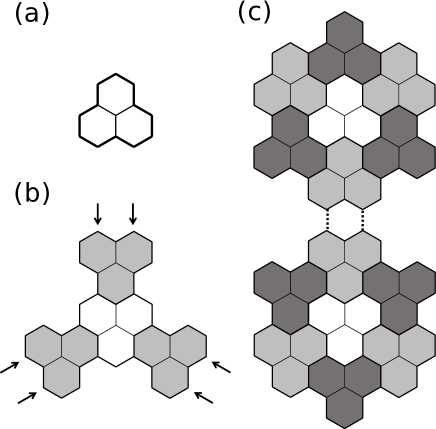
Figure 1: (a) Phenalenyl unit (PU). (b) Example of an ($\alpha$-)phenalenyl-tessellation molecule (PTM). The double zigzag corners (DZCs) are indicated by arrows. (c) Example of a polymerized PTM (poly-PTM). The $\alpha$-PTM (lower) and $\beta$-PTM (upper) are connected at DZCs as indicated by dashed lines.

As depicted in Fig. 1(a), the carbon network is diagrammatically created only from phenalenyl units (PUs). Any poly-PTM has to be created from several phenalenyl-tessellation molecules (PTMs) bonded together by bond connections. However, a PTM is not obtained by chemically bonding phenalenyl molecules together. Rather, a PTM is a special carbon network where the skeleton diagram of one PTM contains PUs identified by separate colors. In one PTM(Fig. 1(b)), two neighboring PUs may share a bond. For example, a PTM may contain a phenalenyl molecule but will not include the triangulene.

After several PTMs are prepared, they can be connected to build a poly-PTM(Fig. 1(c)), where the $\alpha$-PTM and $\beta$-PTM are defined according to the “direction” of the phenalenyl structure.[17] The three benzene rings in a PU form a triangle; an $\alpha$-PTM only has PU triangles directed upward while a $\beta$-PTM only has PU triangles directed downward. The only inter-PTM connections are between an $\alpha$-PTM and $\beta$-PTM, and they are treated as chemical bonds. To stabilize the structure of the poly-PTM, each edge of the whole carbon network needs to be terminated by hydrogen.

To construct a 2D honeycomb network of PTMs, we can select triangular PTMs as the basic building block. The lattice has a rhombic unit cell with two “super” sites: $\alpha$ and $\beta$. The $\alpha$-PTM is defined according to whether the triangle (note that this does not correspond to the triangle of PUs) is directed upward or downward. Meanwhile, the $\beta$-PTM is defined as the mirror image of the $\alpha$-PTM. Then, the $\alpha$-PTMs and $\beta$-PTMs are arranged at two sub-lattice sites of a super-honeycomb lattice. Neighboring carbon sites are then connected to create a 2D honeycomb network of PTMs, which becomes the poly-PTM.

Creating additional vacancies in the poly-PTM can obtain unique electronic characteristics. If an atomic vacancy is created at the center of one PU, a localized electronic state with a nonbonding nature appears accordingly. Interestingly, the localized state is centered at the vacancy, and its eigenenergy comes just at or around the Fermi level along the energy axis. Thus, the vacancy-centered localized mode can be defined as a zero mode with a nonbonding nature. Because the number of vacancies is the same as the number of localized zero modes, we can obtain multiple zero modes.

Fig. 2 shows three examples of poly-PTMs with a honeycomb lattice of zero modes. Fig. 2(a) shows a 2D nanographene network comprising an $\alpha$-PTM with four PUs. Three PUs surround one PU to create a triangular PTM. Three vacancies are at the vertices of the triangle. The vacancy-created $\beta$-PTM is a mirror image of the $\alpha$-PTM with three vacancies. In Fig. 2 (b) and (c), $\alpha$-PTM is given by another molecular structure with 7 PUs. Three vacancies are created at centers of three units. Therefore, we call this $\alpha$-PTM with vacancies as a vacancy-created armchair nanographene molecule A (VANG-A) for the structure of Fig. 2 (b) and VANG-B for another structure of Fig. 2 (c). Similar to the 2D nanographene, poly-PTMs are given starting from VANG-A (or VANG-B) in VANG-A nanographene (or VANG-B nanographene) of Fig. 2 (b) (or (c)).

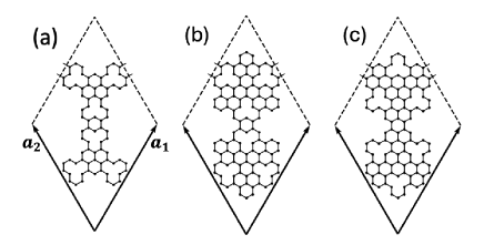
Figure 2: Designed 2D carbon frameworks: (a)2D nanographene (b)VANG-A nanographene (c)VANG-B nanographene. ${\bf a}_{1}$ and ${\bf a}_{2}$ are the lattice vectors.

2.2 The $\pi$-electron model

Here, we present the simplest model for poly-PTM and briefly review its nature. One $\pi$ orbit is at each site of the skeleton diagram, and only the nearest neighbor transfer terms are considered. This obtains the single-orbit tight-binding model (so-TBM). If we assume that the electron transfer Hamiltonian has a non-zero contribution only among nearest-neighbor pairs of $\pi$ sites and that the transfer amplitudes are the same, we can define the so-TBM for the frameworks in Fig. 2. We can then perform dispersion relation calculations of the so-TBM to obtain the band structures, as shown in Fig. 3.

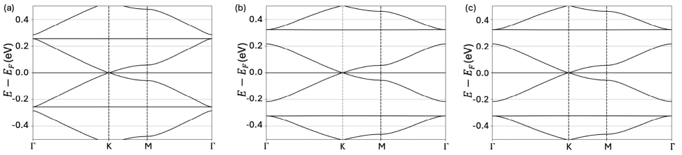
Figure 3: Band structures of so-TBM for (a)2D nanographene, (b)VANG-A nanographene, and (c)VANG-B nanographene.

The localized zero modes at $E_{F}=0$ can be confirmed precisely from the band structures obtained from any molecular framework in Fig. 2 because flat bands with no dispersion appear at the zero energy. All three molecular frameworks have six flat bands at zero energy, which correspond to the localized zero mode for each of the six atom vacancies in a unit cell. This characteristic can be predicted by the super-zero-sum rule.[17] A Dirac point appears at the K (or K’) point where a conduction band and valence band touch.

Owing to the weak inter-electron interaction at each $\pi$ site (i.e., the onsite Hubbard interaction) $U_{\pi}$, we can obtain a single-orbit Hubbard model (so-HM). Here, we consider the following Hamiltonian:

$$H_{\rm so-HM}=-t_{\pi}\sum_{\langle i,j\rangle,\sigma}\left(c^{\dagger}_{i,\sigma}c_{j,\sigma}+{\rm H.c.}\right)+U_{\pi}\sum_{i}n_{i,\uparrow}n_{i,\downarrow},$$ (1)

where $c_{i(j),\sigma}$ and $c^{\dagger}_{i(j),\sigma}$ represent the annihilation and creation, respectively, of an electron with spin $\sigma\in\{\uparrow,\downarrow\}$ at site $i(j)$ and $n_{i,\sigma}=c^{\dagger}_{i,\sigma}c_{i,\sigma}$ is a number operator. Each $\pi$-site is denoted by an integer $i$, and $\sigma$ represents the electron spin. The nearest neighbor sites are connected by a transfer term whose transfer parameter $t_{\pi}$ is assumed to be a constant for any pair of nearest neighbor sites $i$ and $j$. Based on the uniform density theorem, we can eliminate the possibility of charge-segregation and/or charge density waves in the lattice of zero modes in the so-HM.[23]

Interestingly, when the electron number is the same as the number of sites in the so-TBM, the chemical potential comes at the zero modes, which is adjusted at the center of the $\pi$ bands. Then, the zero modes of the so-HM can be expected to be half-filled as well. This is consistent with the chemical picture of NBMOs in alternant hydrocarbon systems. All $\pi$ bands can be separated into bonding, antibonding and nonbonding bands. Under stable conditions, the lower bonding bands are filled by electrons completely. The zero mode, which is a nonbonding mode at $E_{F}$, should appear just between bonding and antibonding bands and become half-filled.

Each zero mode is localized around one of the vacancy sites. If one of the localized zero modes is not half-filled, then the total occupation of the $\pi$ orbital should be non-uniform, which contradicts the uniform density theorem. Thus, the appearance of half-filled zero modes is implied when we consider $U_{\pi}$ as a weak but finite perturbation of the so-TBM. When the interaction $U_{\pi}$ is too large, then obtaining zero modes is difficult although the occupation of $\pi$ sites is uniform.

A half-filled zero mode may show a strong electron correlation effect, which can cause interesting magnetism. Here, we consider the magnetism of the Hubbard model with regard to the $\pi$-network of a poly-PTM. Let the $\alpha$-PTM be one of the poly-PTMs in Fig. 2. Each skeleton diagram of the PTM is bipartite, which means that we can divide $\pi$ sites into A-sites and B-sites. Then, the magnetic ground state may be understood by adopting the Lieb theorem for the repulsive Hubbard model with $U_{\pi}>0$.[24] This approach is not necessarily strong enough to draw conclusions on the quality of the material design, but it can help with clarifying the physical mechanism of magnetism in nanographene.

If we define B-sites as including the center site of a PU, then the number of B-sites $N_{B}$ is two less than the number of A-sites $N_{A}$ because the B-sites have three vacancies. If the Hubbard model is given for each fragment (i.e., one PTM) of the poly-PTM, then because the ground state total spin $S$ is proportional to the difference, it becomes $S=|N_{A}-N_{B}|/2=1$ for one $\alpha$-PTM. Because one $\alpha$-PTM has three localized zero modes and one delocalized zero mode,[22] a natural explanation to make $S=1$ for the ground state is that three of the four zero modes should have parallel electron spins while the fourth electron has an anti-parallel spin.

If we consider a dimer comprising an $\alpha$-PTM and $\beta$-PTM and construct a so-TBM or Hubbard model for the dimer, then we can see that six localized zero modes appear, and there is no delocalized zero mode. According to Lieb’s theorem, the total spin then becomes zero.

These results can be explained consistently in terms of perturbation theory. Three zero modes in one PTM can be represented by three orthogonal wave functions. Each localized orbit is centered at one of the vacancies. Any pair of the three localized orbits has an overlap between two orbits at several carbon $\pi$ sites. This results in a finite positive matrix element of the Hubbard interaction for any two electrons with anti-parallel spins.

The spin states of the three electrons can be given as the spin eigenstates $S=1/2$ or $S=3/2$. Any $S=1/2$ state suffers from the Hubbard interaction, and its energy increases by $U$. In contrast, the $S=3/2$ state has a parallel spin, and there is no energy increase by the Hubbard interaction owing to the Pauli principle. Therefore, the first-order perturbation of three-electron states in the three localized zero modes implies that the lowest energy state has a parallel spin $S=3/2$.

According to the so-TBM, localized zero modes appear as zero-energy eigenstates of the poly-PTM as well as zero modes of an isolated PTM. The number of delocalized zero modes is influenced and determined by the strength of the inter-PTM electron transfer integrals. In contrast, the localized zero modes of the poly-PTM are not affected by the inter-PTM transfer within the so-TBM, which does not consider next-nearest-neighbor transfer integrals.

As an example, consider a dimer comprising one $\alpha$-PTM and one $\beta$-PTM. A small inter-PTM transfer makes the two delocalized zero modes in each PTM hybridize to form a bonding state and antibonding state. These hybridized states are lifted along the energy axis from the zero energy. Then, we can adopt the perturbation approach with $U$ as the perturbation Hamiltonian and only consider electrons in the localized zero modes. Then, we can explain the spin-polarization mechanism hidden in the $S=0$ ground state of the PTM dimer by using the Lieb theorem.

Suppose that the inter-PTM bonds are another perturbation in a poly-PTM skeleton. Among the three localized zero modes on one PTM, the first-order perturbation in the Hubbard interaction results in three parallel spins as discussed above. Thus, two $S=3/2$ spins in these nanographene fragments are coupled antiferromagnetically to create a total spin state of $S=0$. Therefore, a small inter-PTM transfer creates an antiferromagnetic interaction. However, it cannot be the first order because the inclusion of the inter-PTM transfer keeps each zero mode as an eigenstate of the so-TBM. Therefore, the antiferromagnetic effective interaction is a second- or higher-order transfer term.

Thus, we can conclude that the spins of localized zero modes in one PTM tend to align. Meanwhile, inter-PTM interactions should be antiferromagnetic to maintain consistency with Lieb’s theorem. Thus, the zero modes are expected to impart active electron spins to the nanographene.

However, the above evaluation of the so-HM is not sufficient for evaluating real hydrocarbon systems. One reason is the effect of the long-range component of the Coulomb interaction. Even if it appears as a screened Coulomb interaction, off-diagonal components such as inter-site interactions and the contribution from exchange terms are essential for evaluating real materials. These components are not explicitly considered in the so-HM, so it may not be enough to represent the effective magnetic interaction of real materials.

Another reason is inter-zero mode hopping terms, which can appear as hybridization among designed zero modes. Magnetic interactions among electrons accommodated by a zero mode may only happen indirectly via induced spin polarization in the other bonding $\pi$ bands. Therefore, they can appear only as higher-order perturbation terms, which have a weak influence. Thus, another modeling approach is needed starting from the designed hydrocarbon system to obtain stronger conclusions on the resultant magnetism than can be obtained from the so-HM of the $\pi$-electron model.

2.3 Design of magnetic nanographene based on density functional theory

DFT simulations of the electronic structure allowed us to proceed from evaluating the stability of the material structure to determining the effective electron model. With this approach, we can change the skeleton diagram to the proper atomic configuration of the hydrocarbons. The stability of the obtained material can then be tested by simulations to optimize the structure. A stable material according to DFT simulations can confirm the expected appearance of zero modes. Deriving an effective electron model can clarify whether the material realizes the target spin system.

Thus, we created a molecular model of hydrogenated nanographene based on the molecular skeleton (Fig. 4) and calculated the electronic state using DFT simulations to determine the dispersion relation, Wannier functions, and electron transfer Hamiltonian.

Designing a specific atomic configuration of nanographene to have the expected magnetic properties requires several important choices and methods for confirming the appearance of zero modes.

A localized zero mode centered at the center site of a PU can be realized in two ways. One is to create a hydrogenated vacancy. The triply hydrogenated vacancy (i.e., V₁₁₁) is a proper solution,[25] but its creation strongly deforms the graphene framework. The other way is to create a vacancy in the graphitic carbon system by facilitating on-top hydrogen adsorption.[10] We selected on-top hydrogen adsorption because it distorts the graphene structure less and should be easier to handle in real experiments.

The key steps of our design method are as follows:

1. Carbon atoms are placed at the vertices of the skeleton diagram of the poly-PTM shown in Fig. 2.

2. Carbon atoms are placed in the vacancies of the skeleton under the assumption that on-top hydrogen adsorption takes place at these carbon sites.

3. The edges of the nanographene network are assumed to terminate in hydrogen atoms.

Next, we present the following cautions regarding the designed molecules:

1. Edge termination of poly-PTM is assumed to be done by hydrogen atoms. This condition might cause a steric hindrance effect. The flatness of nanographene is disturbed and corrugation in a graphitic $sp^{2}$ structure occurs. We had better confirm whether each polymer of PTMs may suffer from the steric hindrance, or not.

2. By finding the appearance of the corresponding localized electron wave as a dispersion-less band, making Wannier functions of this flat band, we can confirm the existence of zero modes by finding one-to-one correspondence of the Wanner function and a zero mode of so-TBM. By adopting the Wannierization,[20] we can directly derive the zero mode wave function when we find flat bands. Through the Wannierization, a transfer Hamiltonian, i.e. the tight-binding model, is determined. This tight-binding Hamiltonian is called the zero-mode transfer Hamiltonian. This is another merit of the DFT modeling. Arrangement of the zero modes in a properly ordered way allows us to design magnetic systems which should behave as the 2D Heisenberg $S=3/2$ spin systems.

3. In this article, after determining the tight-binding Hamiltonian, we shall examine conditions in which the effective interaction Hamiltonian leads to the realization of expected spin systems.

2.4 Stability test

DFT simulations can be used to obtain interatomic forces. Stable structures can be searched for by tracking the atomic displacement caused by these forces. To calculate the optimal structure and self-consistent field (SCF), we used the norm-conserving pseudopotentials C.pbe-tm-gipaw.UPF and H.pbe-tm-gipaw.UPF in Quantum ESPRESSO.[26, 27, 28] The calculations were performed at the $\Gamma$ point for a unit cell with a vacuum layer having a width of about 15Å. The kinetic energy cutoff was set to 30 Ry for wave functions and 300 Ry for the charge density and potential.

The norm-conserving pseudopotentials that we used yielded band structures of graphene that were indistinguishable from those obtained using other norm-conserving potentials, so there should be no problem with using them for the calculations.

The material structure was considered stable when the optimization procedure converged to a result. The DFT simulations confirmed the existence of VANG in a supercell and the stability of the structures in Fig. 4.

2.5 Renormalized single-particle Hamiltonian

We adopted the plane-wave expansion method using the pseudopotentials from the DFT simulations. A Bloch wave function can be represented in the form of $\psi_{\bf k}({\bf r})=(1/\sqrt{N})e^{i{\bf k}\cdot{\bf r}}u_{\bf k}({\bf r})$, which is given as a three-dimensional (3D) torus. The torus corresponds to the unit cell $({\bf a}_{1},{\bf a}_{2},{\bf a}_{3})$ for which the periodic function $u_{\bf k}({\bf r})$ is defined. We adopted the discrete Fourier transformation so that $u_{\bf k}({\bf r})$ would be given for a set of mesh points. We used a $(N_{1},N_{1},N_{2})$ mesh for the simulations, where $N_{1}$ and $N_{2}$ are integers and $N$ is the total number of given $G$-mesh points and is defined as $N=N_{1}^{2}N_{2}$. The transformed space is given on the reciprocal lattice (i.e., $G$ mesh), where we reduce the representation space according to the cutoff energy. A $G$ mesh point is accepted when it has less than the cutoff energy. Because we considered a planar material structure using a slab model, we used k-vectors indexed by ${\bf k}=(k_{1},k_{2},0)$.

The low-energy Kohn–Sham wave functions $\psi_{n,{\bf k}}({\bf r})$ are given by a set of eigenvectors of a k-indexed effective Hamiltonian matrix where the integer $n$ is the band index. The eigenenergy is denoted by $\varepsilon_{n,{\bf k}}$. The representation matrix $\left(\psi_{n,{\bf k}}({\bf r})\right)$ determines the renormalization transformation matrix from the plane waves $\exp\{i({\bf k}+{\bf G})\cdot{\bf r}\}$ to the Kohn–Sham wave functions. The size of the matrix is determined by the total number of bands $N_{\rm KS-bands}$, which includes $sp^{2}$-$\sigma$ bands and $\pi$-bands, and the number of accepted $G$ mesh points.

We defined $N_{C}$ and $N_{H}$ as the numbers of carbon atoms and hydrogen atoms, respectively, in the unit cell. We obtained KS solutions with the number of bands $N_{\rm KS-bands}=2N_{C}+N_{H}/2+N_{a}$, which included $sp^{2}$ valence bands and $N_{a}$ number of conduction bands. We were able to obtain $N_{\rm KS-bands}$ bands including all antibonding bands, although these Kohn–Sham solutions may include states in the vacuum slab region.

To determine the so-TBM, $\pi$ sites for each system in Fig. 2 were given by a set of points ${\bf R}_{I}$ ($I=1,\cdots,N_{\rm sites}$) in the unit cell. This integer $N_{\rm sites}$ gives the size of a tight-binding Hamiltonian. The model included $N_{\rm sites}=N_{C}-6$, and the bands included bonding and antibonding $\pi$-bands.

The $\pi$ bands are well defined for the KS bands of (hydro-)carbon materials such as graphene, carbon nanotubes, and nanographene, which are included in polyaromatic hydrocarbons. The $\pi$ bands from the DFT simulations generally corresponded to the bands of so-TBM. In particular, the dispersion curves around $E_{F}$ were similar.

If the band structure features obtained by the DFT simulations match the so-TBM, then a one-to-one correspondence for the low-lying $\pi$ bands validates the so-TBM. In addition, if we can confirm the appearance of so-TBM features such as Dirac cones, flat bands, and the characteristic locations of special topological aspects at specific k points in the Kohn–Sham bands, then the design with respect to the underlying atomic configuration is valid.

In our simulations, we found this correspondence for the three nanographene structures in Fig. 2. Then, the renormalized single-particle Hamiltonian (i.e., zero-mode tight-binding Hamiltonian $H_{\rm Wan-TBM}$) can be defined for these low-lying dispersion curves as follows.

If the DFT simulations find a flat band, its Wannier function can be derived. We adopted the Wannierization method using the wannier90 package for our nanographene structures.[29, 30, 31] A group of spectral bands is accompanied by gaps at the top and bottom, as shown in Fig. 3. This feature was confirmed in the bands from the DFT simulations, as shown in Fig. 5 and Fig. 6. The upper and lower energy windows above and below the Fermi energy ($E_{F}$) were determined to include ten bands for the 2D nanographene and eight bands for VANG-A and VANG-B.

The initial values of the Wannier functions were set with $p_{z}$ orbitals on carbon atoms that bonded with the surface on-top hydrogen and carbon atoms either one level above or one level below the central carbon atom in each PTM. Two Dirac-like modes were included in the low-lying branches considered for each system. For example, the Wannierized bands of the VANG-A or VANG-B models comprised six bands with localized zero modes and two bands with Dirac dispersions.

When the Wannierization method converges, a tight-binding Hamiltonian is obtained:

$$H_{\rm Wan-TBM} = H_{\rm intra-PTM-ZM}+H_{\rm inter-PTM-ZM}$$ (2)

$$+H_{\rm ZM-DM}+H_{\rm DM}.$$

Here, $H_{\rm intra-PTM-ZM}$ represents the hopping terms among the three zero modes in one PTM, $H_{\rm inter-PTM-ZM}$ represents the hopping terms connecting a zero mode to zero modes in the nearest-neighbor PTMs, $H_{\rm ZM-DM}$ represents the hybridization terms between zero modes and Dirac-like modes in the lowest branch, and $H_{\rm DM}$ represents the hopping terms of the Dirac-like modes. We confirmed that long-range hopping terms connecting a zero mode farther than the nearest-neighbor sites to another zero mode were negligible. The simulation results also showed that $H_{\rm ZM-DM}$ was negligible.

When the Wannier function is identified as the zero mode designed in the $\pi$-electron model, we can map the DFT model to the zero-mode model. The spectrum of $H_{\rm Wan-TBM}$ generally differs from the zero energy because of the residual hopping terms $H_{\rm intra-PTM-ZM}+H_{\rm inter-PTM-ZM}$ between Wannier functions. When these three partial Hamiltonians are negligible, the dispersion of the zero modes becomes perfectly flat and degenerates at an energy corresponding to their orbital energy. Among these contributions, $H_{\rm intra-PTM-ZM}$ should be small or smaller than $H_{\rm inter-PTM-ZM}$. Depending on the topology and location where each mode exists, $H_{\rm inter-PTM-ZM}$ can be classified. When $H_{\rm inter-PTM-ZM}$ gives local hybridization between a pair of neighboring zero modes, the flat bands split into bonding and antibonding bands but retain their flatness.

3 Material solutions by DFT-based modeling

We designed hydrogenated nanographene as hydrocarbon polymers (Fig. 4). These molecular structures were derived based on nanographene molecular skeleton diagrams in Fig. 2. Poly-PTMs without vacancies were configured, and hydrogen atoms were then placed at the locations of desired vacancies to deliberately induce localized zero modes as NBMOs on the nanographene.

The lateral size of the simulation cell was fixed into a rhombohedral shape in the planar directions. Thus, each obtained structure was subjected to small internal stresses. Because our main objective was to develop a systematic method for designing these materials, we used slightly stressed structures. We checked that the hydrocarbon structure of the nanographene was flat when only in-plane hydrogen termination was considered. When on-top hydrogen adsorption was used, the planar structure deformed owing to the formation of $sp^{3}$-type bonds between the carbon and adsorbed hydrogen.

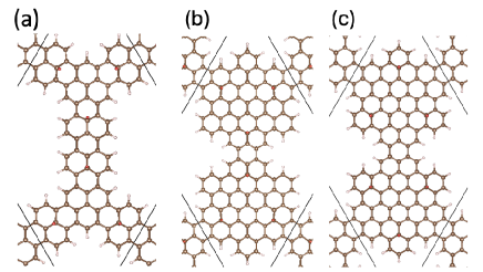
Figure 4: Molecular models of (a)2D nanographene, (b)VANG-A nanographene, and (c)VANG-B nanographene.

3.1 2D nanographene

Fig. 5 displays the band diagram of 2D nanographene obtained through the DFT simulations. Two center bands cross the Fermi level where a point contact (i.e., Dirac point) can be observed at the K point. We defined these bands with Dirac points as Dirac bands. The Fermi energy was determined so that the highest occupied band could be determined by counting electrons. In other words, the system was in the charge-neutral condition when the bonding Dirac band was fully occupied and when the Fermi level came to the Dirac point.

In the vicinity of the Dirac point at the Fermi energy ($E_{F}=0$), six bands with little dispersion were observed, which corresponded to the localized zero modes in the $\pi$-electron model (i.e., NBMOs). The flatness of these bands indicated that highly localized modes appeared. Flat bands also appeared at the bottom and top of the Dirac bands that were in contact at the $\Gamma$ point, which correspond with the results of the so-TBM shown in Fig. 3(a).

The six flat bands had an energy range of $\varepsilon_{n,{\bf k}}$ in $-0.2{\rm eV}\leq\varepsilon_{n,{\bf k}}\leq 0.25{\rm eV}$, which corresponded to the localized modes split into two groups of three. This nearly parallel separation into two bunches of flat bands in the momentum space was an important key for the model. The localized states were interpreted as bonding orbitals and antibonding orbitals made of a pair of zero modes. Two zero modes were attributed to two adjacent PTMs. The energy splitting of $\sim 0.32$ eV was attributed to a next-nearest-neighbor hopping term. However, this term is not explicitly considered in the skeleton diagram, so the split of localized zero modes was not observed in the bands obtained by the so-TBM. This extra electron hopping process can be beneficial for modeling Heisenberg spin systems.

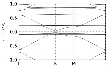
Figure 5: The band structure of 2D nanographene caluclated by DFT.

3.2 Polymerized vacancy-created armchair nanographene

To find localized molecular orbitals, being able to adjust the energy difference of the localized modes is desirable. Therefore, we designed VANG-A and VANG-B as structures with larger and smaller energy splitting. Fig. 6 presents the calculated bands of these structures obtained by DFT simulations.

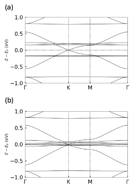
Figure 6: The band structure of (a)VANG-A nanographene and (b)VANG-B nanographene caluclated by DFT.

In VANG-A, bands corresponding to localized zero modes with an energy difference of 0.4081 eV split into two groups of three within $\pm 0.21$ eV of $E_{F}$. In VANG-B, bands corresponding to localized zero modes with an energy difference of 0.1803 eV split into two groups of three within $\pm 0.1$ eV of $E_{F}$.

Fig. 7 and Fig. 8 depict the real-space Wannier functions for VANG-A and VANG-B, respectively. The orbitals in the flat bands could be characterized as NBMOs with alternating signs at each site. Therefore, the orbitals corresponded to the zero modes. We confirmed that the distribution of the wave function amplitude also corresponded to the six localized zero modes of the so-TBM.

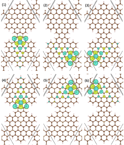
Figure 7: The real-space Wannier functions of the localized zero modes of VANG-A nanographene

Figure 8: The real-space Wannier functions of the localized zero modes of VANG-B nanographene

3.2.1 Analysis of the hopping Hamiltonian

In this study, we started from a design in which three zero modes should appear in one PTM. As a typical example, we placed $\alpha$- and $\beta$-PTMs on a super-honeycomb lattice, which should result in six NBMOs near $E_{F}$. Adjacent PTMs are connected by bonds in the skeleton model, so these NBMOs would not be connected based on the level of approximation of the $\pi$-electron model (i.e., so-TBM). More realistically, multiple transfer paths can appear when a hydrocarbon structure is modeled. Even in the DFT simulates, when we had a localized zero mode centered at an on-top hydrogen atom, two other zero modes should be observed because we had another two localized modes centered at each on-top hydrogen atom. The degeneracy in the orbital energy should be mostly preserved owing to the $C_{3}$ symmetry around the center of each PTM. If orthogonality between three NBMOs in one PTM is maintained, only the transfer between adjacent PTMs should appear.

Let the position vector of a unit cell be given by the 2D lattice vectors ${\bf a}_{1}$ and ${\bf a}_{2}$ (Fig. 2) as ${\bf R}=m_{1}{\bf a}_{1}+m_{2}{\bf a}_{2}$. The two integers $m_{1}$ and $m_{2}$ are in the range $0\leq m_{j}<M$ for $j=1,2$, where $M$ is a large integer.

For VANG-A, the six Wannier orbitals were labeled as $\varphi_{m_{1},m_{2},i}({\bf r})$ with $i=1,2,\cdots,6$. The indices $m_{1}$ and $m_{2}$ specify the unit cell. Typically, the orbital in Fig. 7(1) is $\varphi_{0,0,1}({\bf r})$.

The Wannierization yields a hopping Hamiltonian. We introduced the fully indexed transfer parameters $t_{ij}^{m_{1}m_{2}}$ to represent the transfer from $\varphi_{0,0,i}({\bf r})$ to $\varphi_{m_{1},m_{2},j}({\bf r})$. Owing to the symmetry of the system, we found that many parameters were mutually consistent and could be expressed by a small number of parameters. Table I summarizes the hopping terms obtained by Wannierization. As an example, $\bar{t}=0.0135$eV represents the intra-PTM transfer parameter and is identical to $t_{12}^{00}$, which represents electron hopping from $\varphi_{0,0,1}({\bf r})$ to $\varphi_{0,0,2}({\bf r})$. The value is an order of magnitude smaller than the value of inter-PTM hopping $t=-0.1788$ eV and is identical to $t_{14}^{00}$. These parameters are important where $H_{\rm intra-PTM-ZM}$ and $H_{\rm inter-PTM-ZM}$ are given by $\bar{t}$ and $t$, respectively. Meanwhile, the term of $H_{\rm ZM-DM}$ is negligible because the transfer between any $\varphi_{0,0,i}({\bf r})$ and a Dirac mode is less than $10^{-5}$eV.

Artificial changes to the defined Hamiltonian terms allowed us to apply perturbation theory to several physical arguments. The space of model Hamiltonians has several special points. Suppose that hopping terms among NBMOs are negligible except for $\bar{t}$ and $t$ in the Wannierization results. We also have the limits of $H_{\rm intra-PTM-ZM}=0$ and $H_{\rm inter-PTM-ZM}=0$ given by $\bar{t}=0$ and $t=0$, where Wannier functions for zero modes (i.e., NBMOs) are degenerate at their orbital energy. In VANG-A, the inter-NBMO hybridization by $t_{14}^{00}$ caused the formation of bonding and antibonding states made from $\varphi_{m_{1},m_{2},1}({\bf r})$ and $\varphi_{m_{1},m_{2},4}({\bf r})$ at each ($m_{1}$,$m_{2}$)-th unit cell. If $\bar{t}$ is kept at zero, these newly created modes become the eigenstates of $H_{\rm Wan-TBM}$. Even when $t=-0.1788$eV for all inter-PTM hopping terms, the bonding (and antibonding) states were kept disjointed, and no inter-linking happened between these bonding states. Thus, we obtained two groups of flat bands at $\pm 0.1788$ eV. These result correspond to the split of the central six flat bands into bonding and antibonding bands.

Including a small $\bar{t}$ disperses these flat bands slightly, which explains the results in Fig. 6(a). If the flatness of these bands is preserved, the long-range NBMO-to-NBMO transfer is sufficiently negligible to allow evaluation of the model.

Hopping term							Value[eV]
VANG-A
$\bar{t}$							0.0135
$t$							-0.1788
VANG-B
$\bar{t}$							0.0055
$t$							-0.0214
$t^{\prime}$							-0.0234

Table 1: Evaluation of tight-binding parameters. $t$ and $\bar{t}$ are the inter-PTM transfer integral and intra-PTM transfer integral, respectively. In VANG-B, $t$ and $t^{\prime}$ represent vertical hopping such as $t_{26}^{00}$, and diagonal hopping such as $t_{25}^{00}$, respectively.

The band structures obtained through DFT simulations had various differences between VANG-A and VANG-B that were not apparent in the so-TBM. inter-PTM transfer between localized zero modes obtained through Wannierization was larger for VANG-A, which also had a greater energy difference between localized zero mode bands compared to VANG-B. The larger transfer between localized zero modes for VANG-A can be attributed to the closer surface hydrogen distance within each inter-PTM. This suggests that localized zero modes overlapped more significantly in VANG-A than in VANG-B. The energy difference between zero mode bands is influenced by the magnitude of the inter-PTM transfer, so increasing the inter-PTM transfer can increase the energy difference between localized zero mode bands. Among the band structures (Fig. 6), the localized zero-mode bands of VANG-A exhibited a distinct split but retained their flatness, whereas the localized zero-mode bands of VANG-B were not as split or flat.

If we consider the intra-PTM transfer to be sufficiently small compared to the inter-PTM transfer for VANG-A, electrons are likely to be localized only in a pair of zero modes connected by the inter-PTM transfer. Thus, highly localized and flat bands with energy splitting may appear. In the case of VANG-B, even if we ignore the intra-PTM transfer as in VANG-A, the inter-PTM transfer still connects the entire periodic structure of zero modes. This prevents electrons from localizing, which disperses and bends the flat bands.

3.2.2 Evaluation of inter-electron interaction terms

We adopted the Pariser–Parr–Pople (PPP) method[32] to calculate the electronic Coulomb interaction $U$ and direct exchange interaction $J$ of VANG-A and VANG-B. These parameters were evaluated for the zero modes and not for the $\pi$ orbitals. The PPP method approximates the integral kernels to calculate interactions. To ensure that the long-range Coulomb repulsion behaved inversely proportional to the distance $R$ as $1/R$, we approximated the integral kernel as $1/(1/U_{0}+R)$, where $U_{0}$ represents the onsite Coulomb interaction at a $\pi$ orbital of graphene. We used a value of 9.3 eV obtained from DFT and constrained random-phase approximation (cRPA) calculations of graphene.[33] We assumed that the wave function amplitudes of the Wannierization results at each carbon site could be approximated by the corresponding zero mode of the so-TBM for simplicity. Table II presents the calculation results, where $U$, $U^{\prime}$, and $U^{\prime\prime}$ represent the onsite, intra-PTM, and inter-PTM Coulomb interactions, respectively, such as $U_{1}$, $U^{00}_{12}$, and $U^{00}_{14}$. Here, $U_{i}$ indicates the intra-orbital Coulomb interaction in the $i$th Wannier orbital while $U^{m_{1}m_{2}}_{ij}$ indicates the inter-orbital Coulomb interaction between $\varphi_{0,0,i}({\bf r})$ and $\varphi_{m_{1},m_{2},j}({\bf r})$. $J^{m_{1}m_{2}}_{ij}$ represents the direct exchange interaction between $\varphi_{0,0,i}({\bf r})$ and $\varphi_{m_{1},m_{2},j}({\bf r})$. The value of $J$ represents direct exchange interactions within PTMs, which corresponds to $J^{00}_{12}$.

Interaction term						Value[eV]
VANG-A
$U$						3.829
$U^{\prime}$						1.681
$U^{\prime\prime}$						1.994
$J$						0.031
VANG-B
$U$						3.597
$U^{\prime}$						1.678
$U^{\prime\prime}$						1.267
$J$						0.043

Table 2: Coulomb interaction $U$ and direct exchange interaction $J$ of VANG-A and VANG-B. $U$ represents the onsite Coulomb interaction at a localized zero mode. $U^{\prime}$ represents the Coulomb interaction between zero modes in one PTM (intra-PTM interaction), and $U^{\prime\prime}$ represents the Coulomb interaction between the closest pair of zero modes in neighboring PTMs (inter-PTM interaction). $J$ represents the direct ferromagnetic exchange between Wannier orbitals in one PTM (intra-PTM).

3.2.3 Effective spin Hamiltonian

Based on the above results, we obtained an extended Hubbard Hamiltonian for VANG-A. We referred to the Wannier orbitals $\varphi_{m_{1},m_{2},i}({\bf r})$ to introduce the creation and annihilation operators $c_{m_{1},m_{2},i,\sigma}^{\dagger}$ and $c_{m_{1},m_{2},i,\sigma}$, respectively, for the $i$-th zero modes ($i=1,2,\cdots,6$), where $\sigma=\uparrow,\downarrow$ represents the electron spin. If we neglect hopping terms with smaller transfer parameters than $t$, then the transfer Hamiltonian is given by three major hopping terms:

$$H_{t} = t\sum_{m_{1},m_{2}}\sum_{\sigma}\left(c_{m_{1},m_{2},1,\sigma}^{\dagger}c_{m_{1},m_{2},4,\sigma}+{\rm H.c.}\right)$$ (3)

$$+ t\sum_{m_{1},m_{2}}\sum_{\sigma}\left(c_{m_{1}+1,m_{2},3,\sigma}^{\dagger}c_{m_{1},m_{2},5,\sigma}+{\rm H.c.}\right)$$

$$+ t\sum_{m_{1},m_{2}}\sum_{\sigma}\left(c_{m_{1},m_{2}+1,2,\sigma}^{\dagger}c_{m_{1},m_{2},6,\sigma}+{\rm H.c.}\right).$$

excluding a constant term, the next form is obtained as an extended diagonal Hubbard interaction term:

$$H_{U} = \frac{U}{2}\sum_{m_{1},m_{2}}\sum_{i=1}^{6}:\left(n_{m_{1},m_{2},i,\uparrow}+n_{m_{1},m_{2},i,\downarrow}-1\right)^{2}:$$ (4)

$$+ U^{\prime}\sum_{m_{1},m_{2}}\sum_{\sigma,\sigma^{\prime}}\sum_{\langle i,j\rangle\in S_{1}}\left(n_{m_{1},m_{2},i,\sigma}n_{m_{1},m_{2},j,\sigma^{\prime}}\right)$$

$$+ U^{\prime\prime}\sum_{m_{1},m_{2}}\sum_{\sigma,\sigma^{\prime}}\left(n_{m_{1},m_{2},1,\sigma}n_{m_{1},m_{2},4,\sigma^{\prime}}\right.$$

$$+\left.n_{m_{1}+1,m_{2},3,\sigma}n_{m_{1},m_{2},5,\sigma^{\prime}}+n_{m_{1},m_{2}+1,2,\sigma}n_{m_{1},m_{2},6,\sigma^{\prime}}\right)$$

$$+ {\rm const.}$$

The number operator $n_{m_{1},m_{2},i,\sigma}$ is given by $c^{\dagger}_{m_{1},m_{2},i,\sigma}c_{m_{1},m_{2},i,\sigma}$. Here, $:A:$ represents the normal ordered product of the operator $A$ with respect to the creation and annihilation operators where the order of operators is exchanged using the anti-commutable property so that annihilation operators are on the left of other creation operators. The set of site pairs, $S_{1}$, contains $\langle i,j\rangle=$ $\langle 1,2\rangle$, $\langle 2,3\rangle$, $\langle 3,1\rangle$, $\langle 4,5\rangle$, $\langle 5,6\rangle$, $\langle 6,4\rangle$. In a PTM, there appears inter-zero-mode exchange interaction, which is denoted here by $H_{J}$.

$$H_{J} = -2J\sum_{m_{1},m_{2}}\sum_{\langle i,j\rangle\in S_{1}}\left\{\boldsymbol{S}_{m_{1},m_{2},i}\cdot\boldsymbol{S}_{m_{1},m_{2},j}\right.$$ (5)

$$+ \left.\frac{1}{4}(n_{m_{1},m_{2},i,\uparrow}+n_{m_{1},m_{2},i,\downarrow})(n_{m_{1},m_{2},j,\uparrow}+n_{m_{1},m_{2},j,\downarrow})\right\}.$$

where $\boldsymbol{S}_{m_{1},m_{2},i}$ indicates an S=1/2 spin operator on the Wannier orbital $\varphi_{m_{1},m_{2},i}({\bf r})$.

The total Hamiltonian is given as

$$H=H_{U}+H_{J}+H_{t}.$$ (6)

Here, $U/t$ becomes 21 for VANG-A. As a result, the system is within the strong-correlation limit of the extended Hubbard model. We can treat $H_{U}+H_{J}\equiv H_{0}$ as the non-perturbation terms and $H_{t}\equiv V$ as the perturbation term. The half-filled state of $H_{0}$ is an array of $S=3/2$ spins on a honeycomb lattice. We applied the second-order Rayleigh–Schrödinger perturbation theory to the Hubbard Hamiltonian $H$.[34] The low-energy effective Hamiltonian was then determined as follows:

$$H_{eff}^{(2)}=\sum_{<m,n>}\mathcal{J}\left(\boldsymbol{S}^{(\frac{3}{2})}_{\alpha_{m}}\cdot\boldsymbol{S}^{(\frac{3}{2})}_{\beta_{n}}-\frac{9}{4}\right),\mathcal{J}=\frac{4t^{2}}{9(U-U^{\prime\prime}+2J)}.$$ (7)

Here, $\boldsymbol{S}^{(\frac{3}{2})}_{\alpha_{m}(\beta_{n})}$ represents the spin operator with $S=3/2$ on the m-th $\alpha$-PTM (n-th $\beta$-PTM). By using the obtained values in Table I and Table II, the value of $\mathcal{J}$ was calculated as 0.008 eV. Consequently, the effective Hamiltonian became an antiferromagnetic $S=3/2$ honeycomb Heisenberg model.

The proposed 2D structures based on molecular design exhibited substantial deviations from the anticipated behavior according to the so-TBM. This can be attributed to the presence of a band structure with a split between localized zero modes. Following the design rules, various carbon skeletal structures with localized zero modes can be proposed. For example, a molecular model with a larger carbon array can allow additional positions of surface hydrogen to be chosen more freely compared to nanographene structures such as VANG-A. This would allow for a more selective manipulation of electronic interactions and transfers. By manipulating localized magnetic arrangements and interactions, molecules capable of realizing not only the honeycomb Heisenberg model but also any spin system can be provided.

When we considered terms up to the fourth order, various terms appeared including the bi-quadratic term (BQt) in the RS perturbation.[34, 35] However, BQt is relatively small as a higher-order term compared to the quadratic term in Eq. (7). Methods and strategies for enhancing BQt are discussed elsewhere.

4 Conclusions

We developed a design method that produces a molecular framework so that localized electron wave functions appear spontaneously. In addition to the appearance of the zero modes, magnetic inter-electron interactions can be structured according to the design. We confirmed the design method by DFT simulations to determine the configuration of the localized zero modes. The low-energy electron Hamiltonian evaluated by the Wannierization method naturally determines a transfer Hamiltonian. We present the mechanism by which the inter-electron magnetic interaction causes the occurrence of the spin Hamiltonian as the low-energy effective Hamiltonian.

We present several examples of 2D nanographene structures with localized zero modes constructed through our proposed design method. The DFT simulations and Wannierization results for the nanographene structures identified changes in the band structure around localized zero modes, which can be attributed to distinct variations in the transfer characteristics. Our method uses PTMs with multiple spatially overlapping zero modes, which allows molecular designs that generate enhanced magnetic interactions beyond the mere placement of zero modes as disconnected NBMOs. The ferromagnetic interaction terms that generates large spin moments of $S>1$ are given by spin alignment due to direct exchange interactions because multiple zero modes in the PTM give degenerate orthogonal molecular orbitals with spatial overlap. The effective interaction connecting these localized spin moments with antiferromagnetic interactions is generated by the weak electron transfer between zero modes in adjacent PTMs. Our method results in a Hubbard $U$ term that is tens of times larger than the inter-PTM transfer for zero modes. Thus, the electron system given by the zero-mode array reaches a true strongly correlated state indicating the formation of a stable localized spin state. Considering the electronic correlation effects and electron transfers allowed us to design magnetic structures. The ability of our method to adjust the design and transfer parameters suggests that molecular design is an instrumental tool for developing materials with various magnetic structures, beyond those presented in this study.

References

- [1] R. Raussendorf and H. J. Briegel: Phys. Rev. Lett. 86 (2001) 5188.
- [2] M. A. Nielsen: Phys. Rev. Lett. 93 (2004) 040503.
- [3] N. C. Menicucci, P. van Loock, M. Gu, C. Weedbrook, T. C. Ralph, and M. A. Nielsen: Phys. Rev. Lett. 97 (2006) 110501.
- [4] D. N. Biggerstaff, R. Kaltenbaek, D. R. Hamel, G. Weihs, T. Rudolph, and K. J. Resch: Phys. Rev. Lett. 103 (2009) 240504.
- [5] S. López-Aguayo, Y. V. Kartashov, V. A. Vysloukh, and L. Torner: Phys. Rev. Lett. 105 (2010) 013902.
- [6] S. E. Economou, N. Lindner, and T. Rudolph: Phys. Rev. Lett. 105 (2010) 093601.
- [7] S. D. Bartlett, G. K. Brennen, A. Miyake, and J. M. Renes: Phys. Rev. Lett. 105 (2010) 110502.
- [8] T.-C. Wei, I. Affleck, and R. Raussendorf: Phys. Rev. Lett. 106 (2011) 070501.
- [9] M. Koch-Janusz, D. I. Khomskii, and E. Sela: Phys. Rev. Lett. 114 (2015) 247204.
- [10] N. Morishita, Y. Oishi, T. Yamaguchi, and K. Kusakabe: Applied Physics Express 14 (2021) 121005.
- [11] J. C. G. Henriques and J. Fernández-Rossier: Phys. Rev. B 108 (2023) 155423.
- [12] J. Henriques, M. Ferri-Cortés, and J. Fernández-Rossier: Nano Letters 24 (2024) 3355.
- [13] W. T. Borden and E. R. Davidson: Journal of the American Chemical Society 99 (1977) 4587.
- [14] N. Shima and H. Aoki: Phys. Rev. Lett. 71 (1993) 4389.
- [15] W. T. Borden: Molecular Crystals and Liquid Crystals Science and Technology. Section A. Molecular Crystals and Liquid Crystals 232 (1993) 195.
- [16] A. I. Yuriko Aoki: International Journal of Quantum Chemistry 74 (1999) 491.
- [17] N. Morishita and K. Kusakabe: Physics Letters A 408 (2021) 127462.
- [18] P. Hohenberg and W. Kohn: Phys. Rev. 136 (1964) B864.
- [19] W. Kohn and L. J. Sham: Phys. Rev. 140 (1965) A1133.
- [20] N. Marzari and D. Vanderbilt: Phys. Rev. B 56 (1997) 12847.
- [21] N. Morishita, G. K. Sunnardianto, S. Miyao, and K. Kusakabe: Journal of the Physical Society of Japan 85 (2016) 084703.
- [22] N. Morishita and K. Kusakabe: Journal of the Physical Society of Japan 88 (2019) 124707.
- [23] E. H. Lieb, M. Loss, and R. J. McCann: Journal of Mathematical Physics 34 (1993) 891.
- [24] E. H. Lieb: Phys. Rev. Lett. 62 (1989) 1201.
- [25] M. Ziatdinov, S. Fujii, K. Kusakabe, M. Kiguchi, T. Mori, and T. Enoki: Phys. Rev. B 89 (2014) 155405.
- [26] P. Giannozzi, O. Baseggio, P. Bonfà , D. Brunato, R. Car, I. Carnimeo, C. Cavazzoni, S. de Gironcoli, P. Delugas, F. Ferrari Ruffino, A. Ferretti, N. Marzari, I. Timrov, A. Urru, and S. Baroni: The Journal of Chemical Physics 152 (2020) 154105.
- [27] P. Giannozzi, O. Andreussi, T. Brumme, O. Bunau, M. B. Nardelli, M. Calandra, R. Car, C. Cavazzoni, D. Ceresoli, M. Cococcioni, N. Colonna, I. Carnimeo, A. D. Corso, S. de Gironcoli, P. Delugas, R. A. DiStasio, A. Ferretti, A. Floris, G. Fratesi, G. Fugallo, R. Gebauer, U. Gerstmann, F. Giustino, T. Gorni, J. Jia, M. Kawamura, H.-Y. Ko, A. Kokalj, E. Küçükbenli, M. Lazzeri, M. Marsili, N. Marzari, F. Mauri, N. L. Nguyen, H.-V. Nguyen, A. O. de-la Roza, L. Paulatto, S. Poncé, D. Rocca, R. Sabatini, B. Santra, M. Schlipf, A. P. Seitsonen, A. Smogunov, I. Timrov, T. Thonhauser, P. Umari, N. Vast, X. Wu, and S. Baroni: Journal of Physics: Condensed Matter 29 (2017) 465901.
- [28] P. Giannozzi, S. Baroni, N. Bonini, M. Calandra, R. Car, C. Cavazzoni, D. Ceresoli, G. L. Chiarotti, M. Cococcioni, I. Dabo, A. D. Corso, S. de Gironcoli, S. Fabris, G. Fratesi, R. Gebauer, U. Gerstmann, C. Gougoussis, A. Kokalj, M. Lazzeri, L. Martin-Samos, N. Marzari, F. Mauri, R. Mazzarello, S. Paolini, A. Pasquarello, L. Paulatto, C. Sbraccia, S. Scandolo, G. Sclauzero, A. P. Seitsonen, A. Smogunov, P. Umari, and R. M. Wentzcovitch: Journal of Physics: Condensed Matter 21 (2009) 395502.
- [29] A. A. Mostofi, J. R. Yates, Y.-S. Lee, I. Souza, D. Vanderbilt, and N. Marzari: Computer Physics Communications 178 (2008) 685.
- [30] A. A. Mostofi, J. R. Yates, G. Pizzi, Y.-S. Lee, I. Souza, D. Vanderbilt, and N. Marzari: Computer Physics Communications 185 (2014) 2309.
- [31] G. Pizzi, V. Vitale, R. Arita, S. Blügel, F. Freimuth, G. Géranton, M. Gibertini, D. Gresch, C. Johnson, T. Koretsune, J. Ibañez-Azpiroz, H. Lee, J.-M. Lihm, D. Marchand, A. Marrazzo, Y. Mokrousov, J. I. Mustafa, Y. Nohara, Y. Nomura, L. Paulatto, S. Poncé, T. Ponweiser, J. Qiao, F. Thöle, S. S. Tsirkin, M. Wierzbowska, N. Marzari, D. Vanderbilt, I. Souza, A. A. Mostofi, and J. R. Yates: Journal of Physics: Condensed Matter 32 (2020) 165902.
- [32] K. Nakada, M. Igami, and M. Fujita: Journal of the Physical Society of Japan 67 (1998) 2388.
- [33] T. O. Wehling, E. Şaşıoğlu, C. Friedrich, A. I. Lichtenstein, M. I. Katsnelson, and S. Blügel: Phys. Rev. Lett. 106 (2011) 236805.
- [34] I. Lindgren and J. Morrison: Atomic Many-Body Theory (Springer-Verlag, Berlin, 1982).
- [35] M. Hoffmann and S. Blügel: Phys. Rev. B 101 (2020) 024418.