A Two-layer Stochastic Game Approach to Reinsurance Contracting and Competition

Zongxia Liang Department of Mathematical Sciences, Tsinghua University, Beijing 100084, China. E-mail: liangzongxia@tsinghua.edu.cn    Yi Xia Corresponding author. Department of Mathematical Sciences, Tsinghua University, Beijing 100084, China. E-mail: xia-y20@mails.tsinghua.edu.cn    Bin Zou Department of Mathematics, University of Connecticut, USA. E-mail: bin.zou@uconn.edu
Abstract

We introduce a two-layer stochastic game model to study reinsurance contracting and competition in a market with one insurer and two competing reinsurers. The insurer negotiates with both reinsurers simultaneously for proportional reinsurance contracts that are priced using the variance premium principle; the reinsurance contracting between the insurer and each reinsurer is modeled as a Stackelberg game. The two reinsurers compete for business from the insurer and optimize the so-called relative performance, instead of their own surplus; the competition game between the two reinsurers is settled by a non-cooperative Nash game. We obtain a sufficient and necessary condition, related to the competition degrees of the two reinsurers, for the existence of an equilibrium. We show that the equilibrium, if exists, is unique, and the equilibrium strategy of each player is constant, fully characterized in semi-closed form. Additionally, we obtain interesting sensitivity results for the equilibrium strategies through both an analytical and numerical study.

Key words: Game theory; Stackelberg game; Non-cooperative Nash game; Optimal reinsurance; Relative performance

1 Introduction

Insurers play a critical role in maintaining the financial stability of households and businesses, but they also face significant claim risks that can threaten their solvency. To mitigate these risks, insurers can diversify their insurance portfolios through reinsurance. Of course, when reinsurers offer reinsurance coverage to insurers, their goal is not solely to help insurers maintain solvency but also to generate profit from such businesses. As the customers of reinsurance are relatively limited, especially when comparing to those of regular insurance policies, reinsurers naturally compete for those limited customers (insurers), and the competition in turn motivates reinsurers to take into account the competitors’ strategies in their own decision making. To capture the contract negotiation and business competition in the reinsurance market, we propose a two-layer stochastic game model with one insurer and two reinsurers, and aim to obtain an equilibrium for such a complex game. The topic of optimal reinsurance is well studied in the actuarial literature, and papers on dynamic reinsurance often differ in contract types, risk models, premium rules, optimization criteria (preferences), and additional controls (such as investment and dividend decisions). The two dominate reinsurance contracts are excess-of-loss reinsurance (see Asmussen et al., (2000)) and proportional reinsurance, also called quota-share reinsurance (see Schmidli, (2001)). Regarding the insurer’s risk exposure, a standard choice is the classical Cramér-Lundberg model (see Schmidli, (2002)), but its approximating diffusion model is equally popular (see Asmussen et al., (2000) and Schmidli, (2001)). When it comes to the premium principles, the expected value principle is arguably the most common option (see Schmidli, (2001)), and the variance principle is another popular choice (see Chi, (2012) and Liang and Yuen, (2016)). Further generalizations include the mean-CVaR premium principle (see Tan et al., (2020)) and extended distortion premium principles (see Jin et al., (2024)). Early works often adopt maximizing expected utility or minimizing ruin probability as their optimization criterion, but mean-variance preferences are also frequently used (see Li et al., (2015)). Several recent papers take into account ambiguity in modeling and apply different ambiguity preferences in the study (see Gu et al., (2018) for the worst-case approach and Zhang and Li, (2021) for the α𝛼\alpha-maxmin preferences). Risk constraints, such as VaR and CVaR (CTE), can be incorporated so that the obtained optimal contracts help insurers meet the regulatory requirements in practice (see Tan et al., (2009) and Lu et al., (2016)). Last, we mention that some recent contributions to this topic include novel features in their models; for instance, Gu et al., (2018) allow the insurer to invest their surplus in a financial market to explore statistical arbitrages caused by mispricing of stocks, and Peng et al., (2021) consider an insurer who possesses inside information on the asset prices. We refer interested readers to Cai and Chi, (2020) for a review article and Albrecher et al., (2017) for a monograph on optimal reinsurance. Traditionally, research on optimal reinsurance takes the viewpoint of the insurer and seeks an optimal reinsurance contract that optimizes the insurer’s objective; see those reviewed above for evidence. However, both parties of a reinsurance contract come to an agreement through bargaining and negotiations. As such, to better describe the negotiation process, we should propose models that can capture the strategic interplay between the insurer and reinsurer of a contract. One obvious solution is to apply game theory and seek an equilibrium contract that takes into account the interests of both parties at the same time. Indeed, there has been a burgeoning interest to model reinsurance contracting as a game in recent years. Jiang et al., (2019) introduce a two-person cooperative game and solve it to obtain the equilibrium reinsurance contract. On the other hand, Chen and Shen, (2018, 2019) model the reinsurance contracting as a Stackelberg game, which is a type of noncooperative game. In this work, we adopt a game approach to study reinsurance contracting problems. In particular, we follow Chen and Shen, (2018) and model reinsurance contracting as a dynamic Stackelberg game. In such a game, the reinsurer is the leader and chooses the premium principle, while the insurer is the follower and chooses its reinsurance coverage. The hierarchical structure reflects the fact that reinsurers often have more advantages in negotiation; mathematically, this feature implies that the reinsurer knows the insurer’s optimal decision and uses such information in determining its own optimal strategy (premium). We note that the (dynamic) Stackelberg game framework has already received considerable attention since Chen and Shen, (2018, 2019), which are likely the first two papers proposing such a framework. For instance, Li and Young, (2022) generalize Chen and Shen, (2019) to a mean-variance premium principle and a random planning horizon; Cao et al., (2022) consider a general Lévy risk process and allow the insurer and reinsurer to have heterogeneous, ambiguous beliefs on the risk distribution. However, the Stackelberg game model for reinsurance discussed earlier (see Chen and Shen, (2018, 2019), Li and Young, (2022), and Cao et al., (2022)) only considers the simple case of one insurer and one reinsurer, and thus cannot capture the observed fact that insurers often seek reinsurance coverage from multiple reinsurers at the same time.111Reinsurers also compete with each other to win business from large insurers, as argued in Boonen et al., (2021) and Zhu et al., (2023). A minimum model that is consistent with this fact should consist of one insurer and two reinsurers; one of such models is proposed in Cao et al., 2023b . In that paper, the insurer faces two Stackelberg reinsurance games, and its optimal reinsurance strategies depends on the premium rules by both reinsurers in the market (one insurer applies the expected-value principle but the other uses the variance principle). As a result, although the two reinsurers in Cao et al., 2023b are not directly linked, each impacts the other’s decision through the common insurer. Cao et al., 2023b extend the 222-reinsurer model in Cao et al., 2023a to an n𝑛n-reinsurer model, in which all reinsurers apply the variance premium principle. Both Cao et al., 2023a ; Cao et al., 2023b adopt the ambiguity-averse and risk-neutral preferences from Cao et al., (2022) and obtain unique equilibrium strategies for all players. There are also recent works that propose a similar multi-player setup in their game model. Wang et al., (2020) study an asymmetric information linear-quadratic stochastic Stackelberg differential game with one leader and two followers; see also Kroell et al., (2023) for a model with multiple insurers (followers). Bo et al., (2024) consider an insurance market consisting of multiple competing insurers with a mean-field type interaction via the relative performance of their terminal wealth. With the motivations discussed above, we are now ready to present the game model in this paper, which is largely inspired by the one in Cao et al., 2023b . The reinsurance market is composed of one representative insurer and two competing reinsurers, who both apply the variance premium principle,222Chi, (2012) studies optimal reinsurance under variance related premium principles and argues that they form a crucial family of premium principles in actuarial science. We comment that the variance principle is indeed frequently used in the study of optimal reinsurance problems; see Zhou and Yuen, (2012), Chen et al., (2016), Liang and Yuen, (2016), Chen and Shen, (2019), and Cao et al., 2023a ; Cao et al., 2023b for a short list. but possibly with different loading factors, to price their reinsurance contracts. The insurer seeks proportional reinsurance contracts from both reinsurers simultaneously and thus faces two parallel Stackelberg reinsurance games. Given the variance loading factors θ=(θ1,θ2)𝜃subscript𝜃1subscript𝜃2\theta=(\theta_{1},\theta_{2}), the insurer’s goal is to find its optimal reinsurance ceded proportions (p¯1(θ),p¯2(θ))subscript¯𝑝1𝜃subscript¯𝑝2𝜃(\bar{p}_{1}(\theta),\bar{p}_{2}(\theta)), in which p¯i(θ)subscript¯𝑝𝑖𝜃\bar{p}_{i}(\theta) is the optimal proportion ceded to Reinsurer i𝑖i, i=1,2𝑖12i=1,2, and, as imagined, depends on the two reinsurers’ joint premium strategy θ𝜃\theta. The two reinsurers in Cao et al., 2023b compete in an indirect way, but here they compete directly. To be precise, Reinsurer i𝑖i in our model does not optimize its own surplus, Xi(T)subscript𝑋𝑖𝑇X_{i}(T), at the terminal time T𝑇T, but compares its wealth to Xj(T)subscript𝑋𝑗𝑇X_{j}(T), the competitor, Reinsurer j𝑗j’s wealth (i,j=1,2formulae-sequence𝑖𝑗12i,j=1,2 and ij𝑖𝑗i\neq j); by following Bensoussan et al., (2014), we define the so-called relative performance Xi(T)λiXj(T)subscript𝑋𝑖𝑇subscript𝜆𝑖subscript𝑋𝑗𝑇X_{i}(T)-\lambda_{i}X_{j}(T), in which λi0subscript𝜆𝑖0\lambda_{i}\geq 0, and assume that Reinsurer i𝑖i optimizes its relative performance as a way to model direct competition. Therefore, the two reinsurers in our model interact via two channels: the relative performance in their optimization criterion and the feedback response from the insurer; we note that Cao et al., 2023b only consider the latter channel. To settle the competition game, we resort to the notion of classical non-cooperative Nash game, in which the two reinsurers make decisions simultaneously. To summarize, we propose a novel two-layer stochastic game model to study reinsurance contracting and competition, with the former by two parallel Stackelberg games and the latter by a non-cooperative Nash game. All three players are utility maximizers, and we further assume that their preferences are given by an exponential, also called CARA (Constant Absolute Risk Aversion) utility function. Under the proposed game, the two reinsurers aim to find their equilibrium premium strategy θisuperscriptsubscript𝜃𝑖\theta_{i}^{*}, i=1,2𝑖12i=1,2, and the insurer seeks an equilibrium reinsurance strategy p=(p1,p2)superscript𝑝superscriptsubscript𝑝1superscriptsubscript𝑝2p^{*}=(p_{1}^{*},p_{2}^{*}). The key findings and contributions of this paper are discussed as follows. First, we propose a novel two-layer game model with multiple (two) reinsurers, which incorporates desirable features from at least three types of models: dynamic Stackelberg game models (see Chen and Shen, (2018)), models with multiple reinsurers (see Cao et al., 2023b ), and game models with relative performance (see Bensoussan et al., (2014)). Second, we obtain a sufficient and necessary condition for the existence of a game equilibrium, given explicitly by 0λ1λ2<10subscript𝜆1subscript𝜆210\leq\lambda_{1}\lambda_{2}<1, in which λisubscript𝜆𝑖\lambda_{i} is the competition degree parameter of Reinsurer i𝑖i in its relative performance, i=1,2𝑖12i=1,2. Such a condition is precise and sharp because we show that if λ1λ21subscript𝜆1subscript𝜆21\lambda_{1}\lambda_{2}\geq 1, the proposed game admits no equilibrium. In addition, when 0λ1λ2<10subscript𝜆1subscript𝜆210\leq\lambda_{1}\lambda_{2}<1 holds, the equilibrium is unique, and all equilibrium strategies are constant, even though random (stochastic) strategies are allowed in the mathematical formulation. We are able to fully characterize the equilibrium strategies for all players in semi-closed form, subject to finding a unique fixed point of a bivariate function (such a task is easy from the computational point of view). Third, for the reinsurers’ equilibrium premium strategies, we obtain analytical results on the impact of risk aversion δisubscript𝛿𝑖\delta_{i} and competition degree λisubscript𝜆𝑖\lambda_{i}. We show that the increase of one player’s risk aversion will cause both reinsurers to charge a higher loading under equilibrium, but the competition drives them to lower the premium. We also conduct a numerical study to investigate how those model parameters affect the insurer’s reinsurance decisions. The key findings are that the insurer cedes more risk to reinsurers when its own risk aversion increases or when the reinsurers are less risk averse. The rest of the paper is organized as follows. We introduce the two-layer Stackelberg-Nash game model in Section 2. In Section 3, we solve the equilibrium strategies for all players in the Stackelberg game. We then analyze the equilibrium strategies mathematically and give the economic explanation in Section 4. Section 5 concludes this paper. Several technical proofs are placed in Appendix A.

2 Model

We consider a reinsurance market consisting of one insurer, labeled as Insurer (player) 0, and two competing reinsurers, labeled as Reinsurer (player) 1 and 2, over a finite horizon [0,T]0𝑇[0,T], with T>0𝑇0T>0 denoting the terminal time. To account for the competition between the two reinsurers, we assume that the market is formed under a tree structure as in Cao et al., 2023b ; Cao et al., 2023a ; see Figure 1 for graphic illustration. Under such a market formulation, the insurer negotiates reinsurance contracts with both reinsurers simultaneously, and the two reinsurers compete for business from the insurer. Note that our model includes two degenerate cases in which the insurer only purchases reinsurance from one reinsurer.

Refer to caption
Figure 1: Two-layer Reinsurance Game Model

2.1 Strategies

We assume that the insurer receives income at a constant rate c>0𝑐0c>0 and is exposed to aggregate risks L={L(t),t[0,T]}𝐿𝐿𝑡𝑡0𝑇L=\{L(t),t\in[0,T]\} that follow a standard diffusion model (see, e.g., Schmidli, (2001)). To be precise, the dynamics of the risk exposure L𝐿L is governed by

dL(t)=μdt+σdW(t),d𝐿𝑡𝜇d𝑡𝜎d𝑊𝑡\displaystyle\mathrm{d}L(t)=\mu\,\mathrm{d}t+\sigma\,\mathrm{d}W(t),

in which μ,σ>0𝜇𝜎0\mu,\sigma>0 are the drift and volatility parameters of the insurer’s risk process, respectively, and W={W(t),t[0,T]}𝑊𝑊𝑡𝑡0𝑇W=\{W(t),t\in[0,T]\} is a one-dimensional Brownian motion defined on a filtered, complete probability space (Ω,,𝔽,)Ω𝔽\left(\Omega,\mathcal{F},\mathbb{F},\mathbb{P}\right). Here, 𝔽={(t),t[0,T]}𝔽𝑡𝑡0𝑇\mathbb{F}=\left\{\mathcal{F}(t),{t\in[0,T]}\right\} is the augmentation of the natural filtration generated by W𝑊W and satisfies the usual conditions. Hereafter 𝔼()𝔼\mathbb{E}(\cdot) and 𝕍()𝕍\mathbb{V}(\cdot) denote the expectation and variance operators under \mathbb{P}, respectively. To mitigate the risk exposure, the insurer purchases proportional reinsurance from Reinsurers 1 and 2, with ceded proportions p1={p1(t),t[0,T]}subscript𝑝1subscript𝑝1𝑡𝑡0𝑇p_{1}=\{p_{1}(t),t\in[0,T]\} and p2={p2(t),t[0,T]}subscript𝑝2subscript𝑝2𝑡𝑡0𝑇p_{2}=\{p_{2}(t),t\in[0,T]\}, respectively. That is, at each time t[0,T]𝑡0𝑇t\in[0,T], p1(t)dL(t)subscript𝑝1𝑡d𝐿𝑡p_{1}(t)\mathrm{d}L(t) is ceded to Reinsurer 1, p2(t)dL(t)subscript𝑝2𝑡d𝐿𝑡p_{2}(t)\mathrm{d}L(t) is ceded to Reinsurer 2, while (1p1(t)p2(t))dL(t)1subscript𝑝1𝑡subscript𝑝2𝑡d𝐿𝑡(1-p_{1}(t)-p_{2}(t))\mathrm{d}L(t) is retained by the insurer. To receive the reinsurance coverage, the insurer pays premiums that are computed by the variance premium principle (see, e.g., Chi, (2012) and Liang and Yuen, (2016)). Denoting θi={θi(t),t[0,T]}subscript𝜃𝑖subscript𝜃𝑖𝑡𝑡0𝑇\theta_{i}=\{\theta_{i}(t),t\in[0,T]\} the loading factor of Reinsurer i𝑖i, the premium ci={ci(t),t[0,T]}subscript𝑐𝑖subscript𝑐𝑖𝑡𝑡0𝑇c_{i}=\{c_{i}(t),t\in[0,T]\} for a reinsurance contract with ceded proportion pisubscript𝑝𝑖p_{i} satisfies

ci(t)dt=𝔼(pi(t)dL(t))+θi(t)𝕍(pi(t)dL(t)),i=1,2,formulae-sequencesubscript𝑐𝑖𝑡d𝑡𝔼subscript𝑝𝑖𝑡d𝐿𝑡subscript𝜃𝑖𝑡𝕍subscript𝑝𝑖𝑡d𝐿𝑡𝑖12\displaystyle c_{i}(t)\,\mathrm{d}t=\mathbb{E}\big{(}p_{i}(t)\,\mathrm{d}L(t)\big{)}+\theta_{i}(t)\,\mathbb{V}\big{(}p_{i}(t)\,\mathrm{d}L(t)\big{)},\quad i=1,2,

implying that

ci(t)=μpi(t)+θi(t)σ2pi2(t),i=1,2.formulae-sequencesubscript𝑐𝑖𝑡𝜇subscript𝑝𝑖𝑡subscript𝜃𝑖𝑡superscript𝜎2superscriptsubscript𝑝𝑖2𝑡𝑖12\displaystyle c_{i}(t)=\mu\,p_{i}(t)+\theta_{i}(t)\sigma^{2}p_{i}^{2}(t),\quad i=1,2. (2.1)

Let p:=(p1,p2)assign𝑝subscript𝑝1subscript𝑝2p:=(p_{1},p_{2}) denote the insurer’s proportional reinsurance strategy and θ=(θ1,θ2)𝜃subscript𝜃1subscript𝜃2\theta=(\theta_{1},\theta_{2}) the pair of premium loadings, in which θisubscript𝜃𝑖\theta_{i} is Reinsurer i𝑖i’s premium strategy, i=1,2𝑖12i=1,2. Throughout the paper, we suppress the dependence of processes (e.g., cisubscript𝑐𝑖c_{i} and Xisubscript𝑋𝑖X_{i}) on strategy p𝑝p and/or θ𝜃\theta. Given p𝑝p and θ𝜃\theta, the insurer’s surplus process X0={X0(t),t[0,t]}subscript𝑋0subscript𝑋0𝑡𝑡0𝑡X_{0}=\{X_{0}(t),t\in[0,t]\} follows the dynamics ​

dX0(t)dsubscript𝑋0𝑡\displaystyle\mathrm{d}X_{0}(t) =cdt(1p1(t)p2(t))dL(t)(c1(t)+c2(t))dtabsent𝑐d𝑡1subscript𝑝1𝑡subscript𝑝2𝑡d𝐿𝑡subscript𝑐1𝑡subscript𝑐2𝑡d𝑡\displaystyle=c\,\mathrm{d}t-\big{(}1-p_{1}(t)-p_{2}(t)\big{)}\,\mathrm{d}L(t)-\big{(}c_{1}(t)+c_{2}(t)\big{)}\,\mathrm{d}t (2.2)
=(cμθ1(t)σ2p12(t)θ2(t)σ2p22(t))dt(1p1(t)p2(t))dW(t)absent𝑐𝜇subscript𝜃1𝑡superscript𝜎2superscriptsubscript𝑝12𝑡subscript𝜃2𝑡superscript𝜎2superscriptsubscript𝑝22𝑡d𝑡1subscript𝑝1𝑡subscript𝑝2𝑡d𝑊𝑡\displaystyle=\!\left(c\!-\!\mu\!-\!\theta_{1}(t)\sigma^{2}p_{1}^{2}(t)\!-\!\theta_{2}(t)\sigma^{2}p_{2}^{2}(t)\right)\mathrm{d}t\!-\!\big{(}1-p_{1}(t)\!-\!p_{2}(t)\big{)}\,\mathrm{d}W(t) (2.3)

with X0=x0subscript𝑋0subscript𝑥0X_{0}=x_{0}\in\mathbb{R}. Similarly, we obtain the dynamics of Reinsurer i𝑖i’s surplus process Xi={Xi(t),t[0,t]}subscript𝑋𝑖subscript𝑋𝑖𝑡𝑡0𝑡X_{i}=\{X_{i}(t),t\in[0,t]\} by

dXi(t)=ci(t)dtpi(t)dL(t)=θi(t)σ2pi2(t)dtσpi(t)dW(t)dsubscript𝑋𝑖𝑡subscript𝑐𝑖𝑡d𝑡subscript𝑝𝑖𝑡d𝐿𝑡subscript𝜃𝑖𝑡superscript𝜎2superscriptsubscript𝑝𝑖2𝑡d𝑡𝜎subscript𝑝𝑖𝑡d𝑊𝑡\displaystyle\mathrm{d}X_{i}(t)=c_{i}(t)\,\mathrm{d}t-p_{i}(t)\,\mathrm{d}L(t)=\theta_{i}(t)\sigma^{2}p_{i}^{2}(t)\,\mathrm{d}t-\sigma p_{i}(t)\,\mathrm{d}W(t) (2.4)

with Xi(0)=xisubscript𝑋𝑖0subscript𝑥𝑖X_{i}(0)=x_{i}\in\mathbb{R}, for i=1,2𝑖12i=1,2.

We proceed to define the insurer’s and reinsurers’ admissible strategies below.

Definition 2.1.

We call p=(p1,p2)𝑝subscript𝑝1subscript𝑝2p=(p_{1},p_{2}) an admissible (reinsurance) strategy for the insurer if it satisfies the following conditions:

  • (i)

    p1subscript𝑝1p_{1} and p2subscript𝑝2p_{2} are progressively measurable with respect to Borel([0,])()tensor-productBorel0\text{Borel}([0,\cdot])\otimes\mathcal{F}(\cdot);

  • (ii)

    pi(t)[0,1]subscript𝑝𝑖𝑡01p_{i}(t)\in[0,1], i=1,2𝑖12i=1,2, and p1(t)+p2(t)[0,1]subscript𝑝1𝑡subscript𝑝2𝑡01p_{1}(t)+p_{2}(t)\in[0,1] almost surely (a.s.), for all t[0,T]𝑡0𝑇t\in[0,T].

We call θisubscript𝜃𝑖\theta_{i} an admissible (premium) strategy for Reinsurer i𝑖i, i=1,2𝑖12i=1,2, if it satisfies the following conditions:

  • (i)

    θisubscript𝜃𝑖\theta_{i} is progressively measurable with respect to Borel([0,])()tensor-productBorel0\text{Borel}([0,\cdot])\otimes\mathcal{F}(\cdot);

  • (ii)

    θisubscript𝜃𝑖\theta_{i} is uniformly bounded and positive.

Let 𝒰0subscript𝒰0\mathcal{U}_{0}, 𝒰1subscript𝒰1\mathcal{U}_{1}, and 𝒰2subscript𝒰2\mathcal{U}_{2} denote the set of all admissible strategies for the insurer (Insurer 00), Reinsurer 111, and Reinsurer 222, respectively,333With slight abuse of notation, we also use 𝒰isubscript𝒰𝑖\mathcal{U}_{i}, i=0,1,2𝑖012i=0,1,2, to denote the admissible set at each time t[0,T]𝑡0𝑇t\in[0,T]. and 𝒰:=𝒰0×𝒰1×𝒰2assign𝒰subscript𝒰0subscript𝒰1subscript𝒰2\mathcal{U}:=\mathcal{U}_{0}\times\mathcal{U}_{1}\times\mathcal{U}_{2} denote the joint admissible set of all three players.

As stated in Section 1 (and will be described in detail shortly), we consider a game model with three players; as such, the surplus process of one player not only depends on its own strategy but also on the other two players’. For this reason, we will only consider strategies that are jointly admissible to all players, (p,θ1,θ2)𝒰0×𝒰1×𝒰2𝑝subscript𝜃1subscript𝜃2subscript𝒰0subscript𝒰1subscript𝒰2(p,\theta_{1},\theta_{2})\in\mathcal{U}_{0}\times\mathcal{U}_{1}\times\mathcal{U}_{2}, in the subsequent analysis. Note that given a triplet u:=(p,θ1,θ2)𝒰:=𝒰0×𝒰1×𝒰2assign𝑢𝑝subscript𝜃1subscript𝜃2𝒰assignsubscript𝒰0subscript𝒰1subscript𝒰2u:=(p,\theta_{1},\theta_{2})\in\mathcal{U}:=\mathcal{U}_{0}\times\mathcal{U}_{1}\times\mathcal{U}_{2}, the insurer’s surplus equation (2.3) admits a unique solution X0=X0x0,usubscript𝑋0superscriptsubscript𝑋0subscript𝑥0𝑢X_{0}=X_{0}^{x_{0},u} for each x0subscript𝑥0x_{0}\in\mathbb{R}, and the same is true for Reinsurer i𝑖i’s surplus equation (2.4) under Xi(0)=xisubscript𝑋𝑖0subscript𝑥𝑖X_{i}(0)=x_{i}\in\mathbb{R}, i=1,2𝑖12i=1,2. In Definition 2.1, both the proportional reinsurance strategy p𝑝p of the insurer and the premium strategies θ𝜃\theta of the reinsurers are allowed to be rather general stochastic processes. But in practice, reinsurance contracts are signed and fixed over the life of specified periods, implying that both p𝑝p and θ𝜃\theta are not random but constants. As such, it seems that we should impose such constraints upfront in defining admissible strategies. However, as shown in Theorem 3.3, all strategies under equilibrium are constants even when we consider random strategies as in Definition 2.1. Therefore, we decide not to impose the assumption of constant strategies in Definition 2.1 for the benefit of mathematical generality.

2.2 Games

To start, we assume that all three players, one insurer and two reinsurers, in the market are utility maximizers and further that the preferences of (Re)Insurer i𝑖i are characterized by an exponential function

Ui(x)=1δieδix,i=0,1,2,formulae-sequencesubscript𝑈𝑖𝑥1subscript𝛿𝑖superscriptesubscript𝛿𝑖𝑥𝑖012\displaystyle U_{i}(x)=-\frac{1}{\delta_{i}}\,\mathrm{e}^{-\delta_{i}x},\quad i=0,1,2, (2.5)

in which δi>0subscript𝛿𝑖0\delta_{i}>0 is the (constant) absolute risk aversion parameter. Following Cao et al., 2023b ; Cao et al., 2023a , we model the reinsurance contracting between the insurer and each of the two reinsurers as a Stackelberg game and the competition between two reinsurers as a non-cooperative Nash game. In all games, the information is perfect and symmetric to both parties. In each Stackelberg game, the reinsurer is the leader and chooses its premium strategy θisubscript𝜃𝑖\theta_{i}, and the insurer is the follower and chooses its reinsurance strategy pisubscript𝑝𝑖p_{i}. However, different from these two papers, the competition here is modeled via the so-called relative performance; to be precise, Reinsurer i𝑖i in Cao et al., 2023b optimizes its own surplus (performance) Xisubscript𝑋𝑖X_{i}, i=1,2𝑖12i=1,2, but here it optimizes the relative performance XiλiXjsubscript𝑋𝑖subscript𝜆𝑖subscript𝑋𝑗X_{i}-\lambda_{i}X_{j}, with ji𝑗𝑖j\neq i, in which λi>0subscript𝜆𝑖0\lambda_{i}>0 measures the competition degree of Reinsurer i𝑖i relative to its competitor Reinsurer j𝑗j. The limit case of λ1=λ2=0subscript𝜆1subscript𝜆20\lambda_{1}=\lambda_{2}=0 reduces to the scenario investigated in Cao et al., 2023b ; Cao et al., 2023a and is considered in Section 3.4. As stated above, the insurer, as the follower in each Stackelberg contracting game, seeks an optimal reinsurance strategy in response to the reinsurers’ chosen premiums. This is formally defined below.

Definition 2.2 (Insurer’s Problem).

Let the reinsurers’ premium strategies θ=(θ1,θ2)𝒰1×𝒰2𝜃subscript𝜃1subscript𝜃2subscript𝒰1subscript𝒰2\theta=(\theta_{1},\theta_{2})\in\mathcal{U}_{1}\times\mathcal{U}_{2} be arbitrary but fixed, and (t,x)[0,T]×𝑡𝑥0𝑇(t,x)\in[0,T]\times\mathbb{R}. The insurer seeks an optimal reinsurance strategy p¯=(p¯1,p¯2)¯𝑝subscript¯𝑝1subscript¯𝑝2\bar{p}=(\bar{p}_{1},\bar{p}_{2}) that maximizes its dynamic objective J0θsuperscriptsubscript𝐽0𝜃J_{0}^{\theta} defined by

J0θ(t,x;p)=𝔼[U0(X0(T))|X0(t)=x],superscriptsubscript𝐽0𝜃𝑡𝑥𝑝𝔼delimited-[]conditionalsubscript𝑈0subscript𝑋0𝑇subscript𝑋0𝑡𝑥\displaystyle J_{0}^{\theta}(t,x;p)=\mathbb{E}[U_{0}(X_{0}(T))|X_{0}(t)=x], (2.6)

in which p¯i:=p¯i(θ)assignsubscript¯𝑝𝑖subscript¯𝑝𝑖𝜃\bar{p}_{i}:=\bar{p}_{i}(\theta) may depend on the reinsurers’ strategies pair θ=(θ1,θ2)𝜃subscript𝜃1subscript𝜃2\theta=(\theta_{1},\theta_{2}), and U0subscript𝑈0U_{0} is given by (2.5) with δ0>0subscript𝛿00\delta_{0}>0. Denote the insurer’s value function by

V¯0θ(t,x)=J0θ(t,x;p¯)=supp𝒰0J0θ(t,x;p).superscriptsubscript¯𝑉0𝜃𝑡𝑥superscriptsubscript𝐽0𝜃𝑡𝑥¯𝑝subscriptsupremum𝑝subscript𝒰0superscriptsubscript𝐽0𝜃𝑡𝑥𝑝\displaystyle\bar{V}_{0}^{\theta}(t,x)=J_{0}^{\theta}(t,x;\bar{p})=\sup_{p\in\mathcal{U}_{0}}\,J_{0}^{\theta}(t,x;p). (2.7)

In the Stackelberg contracting game between Reinsurer i𝑖i and the insurer, Reinsurer i𝑖i is the game leader and chooses its premium loading θisubscript𝜃𝑖\theta_{i}, i=1,2𝑖12i=1,2. Given the hierarchical structure of Stackelberg game, the surplus dynamics of Reinsurer i𝑖i in (2.4) holds under the insurer’s optimal reinsurance strategy p¯¯𝑝\bar{p} defined in (2.7); to account for such a fact, we introduce a more precise notation Xip¯superscriptsubscript𝑋𝑖¯𝑝X_{i}^{\bar{p}} for Reinsurer i𝑖i’s surplus process given p=p¯𝑝¯𝑝p=\bar{p}. As each reinsurer compares its own surplus with the competitor’s, we define the relative performance Yi={Yi(t),t[0,T]}subscript𝑌𝑖subscript𝑌𝑖𝑡𝑡0𝑇Y_{i}=\{Y_{i}(t),t\in[0,T]\} of Reinsurer i𝑖i by

Yi(t)=Xip¯(t)λiXjp¯(t),subscript𝑌𝑖𝑡superscriptsubscript𝑋𝑖¯𝑝𝑡subscript𝜆𝑖superscriptsubscript𝑋𝑗¯𝑝𝑡\displaystyle Y_{i}(t)=X_{i}^{\bar{p}}(t)-\lambda_{i}X_{j}^{\bar{p}}(t), (2.8)

for i,j=1,2formulae-sequence𝑖𝑗12i,j=1,2 and ij𝑖𝑗i\neq j, in which λi>0subscript𝜆𝑖0\lambda_{i}>0 measures the competition degree of Reinsurer i𝑖i to its competitor Reinsurer j𝑗j. Note that Reinsurer i𝑖i’s relative performance, Yisubscript𝑌𝑖Y_{i} in (2.8), depends on not only its own premium strategy θisubscript𝜃𝑖\theta_{i} but also its competitor’s θjsubscript𝜃𝑗\theta_{j}.

Definition 2.3 (Reinsurers’ Problem).

Let i,j=1,2formulae-sequence𝑖𝑗12i,j=1,2 with ij𝑖𝑗i\neq j, θj𝒰jsubscript𝜃𝑗subscript𝒰𝑗\theta_{j}\in\mathcal{U}_{j}, and (t,y)[0,T]×𝑡𝑦0𝑇(t,y)\in[0,T]\times\mathbb{R} be given. Reinsurer i𝑖i seeks an optimal premium strategy θ¯i:=θ¯i(θj)assignsubscript¯𝜃𝑖subscript¯𝜃𝑖subscript𝜃𝑗\bar{\theta}_{i}:=\bar{\theta}_{i}(\theta_{j}) that maximizes its dynamic objective Jiθjsuperscriptsubscript𝐽𝑖subscript𝜃𝑗J_{i}^{\theta_{j}} defined by

Jiθj(t,y;θi)=𝔼[Ui(Yi(T))|Yi(t)=y],superscriptsubscript𝐽𝑖subscript𝜃𝑗𝑡𝑦subscript𝜃𝑖𝔼delimited-[]conditionalsubscript𝑈𝑖subscript𝑌𝑖𝑇subscript𝑌𝑖𝑡𝑦\displaystyle J_{i}^{\theta_{j}}(t,y;\theta_{i})=\mathbb{E}\left[U_{i}(Y_{i}(T))|Y_{i}(t)=y\right], (2.9)

in which Uisubscript𝑈𝑖U_{i} is given by (2.5) with δi>0subscript𝛿𝑖0\delta_{i}>0, and Yisubscript𝑌𝑖Y_{i} by (2.8). Denote the value function by

V¯iθj(t,y)=Jiθj(t,y;θ¯i(θj))=supθi𝒰iJiθj(t,y;θi)superscriptsubscript¯𝑉𝑖subscript𝜃𝑗𝑡𝑦superscriptsubscript𝐽𝑖subscript𝜃𝑗𝑡𝑦subscript¯𝜃𝑖subscript𝜃𝑗subscriptsupremumsubscript𝜃𝑖subscript𝒰𝑖superscriptsubscript𝐽𝑖subscript𝜃𝑗𝑡𝑦subscript𝜃𝑖\displaystyle\bar{V}_{i}^{\theta_{j}}(t,y)=J_{i}^{\theta_{j}}(t,y;\bar{\theta}_{i}(\theta_{j}))=\sup_{\theta_{i}\in\mathcal{U}_{i}}\,J_{i}^{\theta_{j}}(t,y;\theta_{i}) (2.10)

for i,j=1,2formulae-sequence𝑖𝑗12i,j=1,2 and ij𝑖𝑗i\neq j.

As is clear from Definition 2.3, Reinsurer i𝑖i’s optimal strategy θ¯i(θj)subscript¯𝜃𝑖subscript𝜃𝑗\bar{\theta}_{i}(\theta_{j}) depends on its competitor’s strategy θjsubscript𝜃𝑗\theta_{j}. The competition between them is settled by a non-cooperative Nash game, which leads to the following definition of the two-layer game equilibrium.

Definition 2.4 (Equilibrium).

Assume that there exists a fixed point, denoted by θ:=(θ1,θ2)assignsuperscript𝜃superscriptsubscript𝜃1superscriptsubscript𝜃2\theta^{*}:=(\theta_{1}^{*},\theta_{2}^{*}), to the mapping (θ1,θ2)(θ¯1(θ2),θ¯2(θ1))maps-tosubscript𝜃1subscript𝜃2subscript¯𝜃1subscript𝜃2subscript¯𝜃2subscript𝜃1(\theta_{1},\theta_{2})\mapsto(\bar{\theta}_{1}(\theta_{2}),\bar{\theta}_{2}(\theta_{1})), and it is admissible (i.e., θ𝒰1×𝒰2superscript𝜃subscript𝒰1subscript𝒰2\theta^{*}\in\mathcal{U}_{1}\times\mathcal{U}_{2}). The equilibrium of the two-layer reinsurance contracting and competition game plotted in Figure 1 consists of the following controls:

  • θ1=θ¯1(θ2)superscriptsubscript𝜃1subscript¯𝜃1superscriptsubscript𝜃2\theta_{1}^{*}=\bar{\theta}_{1}(\theta_{2}^{*}) and θ2=θ¯2(θ1)superscriptsubscript𝜃2subscript¯𝜃2superscriptsubscript𝜃1\theta_{2}^{*}=\bar{\theta}_{2}(\theta_{1}^{*}) are the equilibrium premium strategies of Reinsurer 1 and Reinsurer 2, respectively, and θ=(θ1,θ2)superscript𝜃superscriptsubscript𝜃1superscriptsubscript𝜃2\theta^{*}=(\theta_{1}^{*},\theta_{2}^{*}) forms the Nash equilibrium of the competition game between the two reinsurers;

  • p:=(p1,p2)=(p¯1(θ),p¯2(θ))assignsuperscript𝑝superscriptsubscript𝑝1superscriptsubscript𝑝2subscript¯𝑝1superscript𝜃subscript¯𝑝2superscript𝜃p^{*}:=(p_{1}^{*},p_{2}^{*})=(\bar{p}_{1}(\theta^{*}),\bar{p}_{2}(\theta^{*})) is the insurer’s equilibrium reinsurance strategy in the Stackelberg games with Reinsurers 1 and 2.

3 Equilibrium

In this section, we first solve the insurer’s problem, for a given pair of admissible premiums θ=(θ1,θ2)𝒰1×𝒰2𝜃subscript𝜃1subscript𝜃2subscript𝒰1subscript𝒰2\theta=(\theta_{1},\theta_{2})\in\mathcal{U}_{1}\times\mathcal{U}_{2}, to obtain its optimal strategy p¯(θ)¯𝑝𝜃\bar{p}(\theta) in Section 3.1; next, assuming that the insurer follows p¯(θ)¯𝑝𝜃\bar{p}(\theta), we solve each reinsurer’s problem in Section 3.2; finally, we combine the above results to obtain the equilibrium of the two-layer game model in Section 3.3.

3.1 Insurer’s Problem

Recall that the insurer’s problem is formally defined in Definition 2.2. To solve the insurer’s problem in (2.7), we apply the dynamic programming method (see Fleming and Soner, (2006) and Yong and Zhou, (2012)) and present the solution in the theorem below.

Theorem 3.1.

For every θ=(θ1,θ2)𝒰1×𝒰2𝜃subscript𝜃1subscript𝜃2subscript𝒰1subscript𝒰2\theta=(\theta_{1},\theta_{2})\in\mathcal{U}_{1}\times\mathcal{U}_{2}, the insurer’s optimal reinsurance strategy p¯={(p¯1(t),p¯2(t)),t[0,T]}¯𝑝subscript¯𝑝1𝑡subscript¯𝑝2𝑡𝑡0𝑇\bar{p}=\{(\bar{p}_{1}(t),\bar{p}_{2}(t)),t\in[0,T]\} is given by

p¯1(t)subscript¯𝑝1𝑡\displaystyle\bar{p}_{1}(t) =δ0θ2(t)δ0θ1(t)+δ0θ2(t)+2θ1(t)θ2(t),absentsubscript𝛿0subscript𝜃2𝑡subscript𝛿0subscript𝜃1𝑡subscript𝛿0subscript𝜃2𝑡2subscript𝜃1𝑡subscript𝜃2𝑡\displaystyle=\dfrac{\delta_{0}\theta_{2}(t)}{\delta_{0}\theta_{1}(t)+\delta_{0}\theta_{2}(t)+2\theta_{1}(t)\theta_{2}(t)}, (3.1)
p¯2(t)subscript¯𝑝2𝑡\displaystyle\bar{p}_{2}(t) =δ0θ1(t)δ0θ1(t)+δ0θ2(t)+2θ1(t)θ2(t),absentsubscript𝛿0subscript𝜃1𝑡subscript𝛿0subscript𝜃1𝑡subscript𝛿0subscript𝜃2𝑡2subscript𝜃1𝑡subscript𝜃2𝑡\displaystyle=\dfrac{\delta_{0}\theta_{1}(t)}{\delta_{0}\theta_{1}(t)+\delta_{0}\theta_{2}(t)+2\theta_{1}(t)\theta_{2}(t)}, (3.2)

and its value function V¯0θsuperscriptsubscript¯𝑉0𝜃\bar{V}_{0}^{\theta}, defined in (2.7), is given by

V¯0θ(t,x)=1δ0eδ0x+f0(t),superscriptsubscript¯𝑉0𝜃𝑡𝑥1subscript𝛿0superscriptesubscript𝛿0𝑥subscript𝑓0𝑡\displaystyle\bar{V}_{0}^{\theta}(t,x)=-\frac{1}{\delta_{0}}\,\mathrm{e}^{-\delta_{0}\,x+f_{0}(t)}, (3.3)

for every (t,x)[0,T]×𝑡𝑥0𝑇(t,x)\in[0,T]\times\mathbb{R}, in which δ0>0subscript𝛿00\delta_{0}>0 is the insurer’s absolute risk aversion, and f0subscript𝑓0f_{0} is

f0(t)=tT{δ0(cμσ2[θ1(s)p¯12(s)+θ2(s)p¯22(s)])+12δ02σ2(1p¯12(s)p¯22(s))}ds.subscript𝑓0𝑡superscriptsubscript𝑡𝑇subscript𝛿0𝑐𝜇superscript𝜎2delimited-[]subscript𝜃1𝑠superscriptsubscript¯𝑝12𝑠subscript𝜃2𝑠superscriptsubscript¯𝑝22𝑠12superscriptsubscript𝛿02superscript𝜎21superscriptsubscript¯𝑝12𝑠superscriptsubscript¯𝑝22𝑠differential-d𝑠\displaystyle f_{0}(t)=\int_{t}^{T}\left\{-\delta_{0}\left(c-\mu-\sigma^{2}\left[\theta_{1}(s)\bar{p}_{1}^{2}(s)+\theta_{2}(s)\bar{p}_{2}^{2}(s)\right]\right)+\frac{1}{2}\delta_{0}^{2}\sigma^{2}\left(1-\bar{p}_{1}^{2}(s)-\bar{p}_{2}^{2}(s)\right)\right\}\mathrm{d}s.\quad (3.4)
Proof.

From the dynamics equation of X0subscript𝑋0X_{0} in (2.3), we define the infinitesimal generator 𝒜0(p,θ)vsuperscriptsubscript𝒜0𝑝𝜃𝑣\mathcal{A}_{0}^{(p,\theta)}\,v, for every vC1,2([0,T]×)𝑣superscriptC120𝑇v\in\mathrm{C}^{1,2}([0,T]\times\mathbb{R}) and every (p,θ)𝒰𝑝𝜃𝒰(p,\theta)\in\mathcal{U}, by

𝒜0p,θv(t,x)superscriptsubscript𝒜0𝑝𝜃𝑣𝑡𝑥\displaystyle\mathcal{A}_{0}^{p,\theta}\,v(t,x) =tv(t,x)+(cμθ1(t)p12(t)σ2θ2(t)p22(t)σ2)xv(t,x)absentsubscript𝑡𝑣𝑡𝑥𝑐𝜇subscript𝜃1𝑡superscriptsubscript𝑝12𝑡superscript𝜎2subscript𝜃2𝑡superscriptsubscript𝑝22𝑡superscript𝜎2subscript𝑥𝑣𝑡𝑥\displaystyle=\partial_{t}v(t,x)+\left(c-\mu-\theta_{1}(t)p_{1}^{2}(t)\sigma^{2}-\theta_{2}(t)p_{2}^{2}(t)\sigma^{2}\right)\partial_{x}v(t,x) (3.5)
+12(1p1(t)p2(t))2σ2xxv(t,x),12superscript1subscript𝑝1𝑡subscript𝑝2𝑡2superscript𝜎2subscript𝑥𝑥𝑣𝑡𝑥\displaystyle\quad+\frac{1}{2}\left(1-p_{1}(t)-p_{2}(t)\right)^{2}\sigma^{2}\partial_{xx}v(t,x), (3.6)

in which vsubscript𝑣\partial_{\cdot}v denotes the corresponding partial derivative of v𝑣v with respect to the subscript argument. Then, applying the dynamic programming principle, we obtain that the insurer’s value function V¯0θsuperscriptsubscript¯𝑉0𝜃\bar{V}_{0}^{\theta}, if V¯0θC1,2([0,T]×)superscriptsubscript¯𝑉0𝜃superscriptC120𝑇\bar{V}_{0}^{\theta}\in\mathrm{C}^{1,2}([0,T]\times\mathbb{R}), is a classical solution to the following Hamilton-Jacobi-Bellman (HJB) equation

{supp𝒰0𝒜0(p,θ)v(t,x)=0,v(T,x)=1δ0exp(δ0x).casessubscriptsupremum𝑝subscript𝒰0superscriptsubscript𝒜0𝑝𝜃𝑣𝑡𝑥0otherwise𝑣𝑇𝑥1subscript𝛿0subscript𝛿0𝑥otherwise\begin{cases}\sup\limits_{p\in\mathcal{U}_{0}}\,\mathcal{A}_{0}^{(p,\theta)}\,v(t,x)=0,\\ v(T,x)=-\frac{1}{\delta_{0}}\exp(-\delta_{0}x).\end{cases} (3.7)

To solve (3.7), we consider an ansatz in the form of (3.3), in which f0C1([0,T])subscript𝑓0superscriptC10𝑇f_{0}\in\mathrm{C}^{1}([0,T]) is yet to be determined. With the help of this particular ansatz, we reduce (3.7) into

{infp𝒰0{12σ2δ02(1p1(t)p2(t))2δ0(cμθ1(t)p12(t)σ2θ2(t)p22(t)σ2)}+f0(t)=0,f0(T)=0.casessubscriptinfimum𝑝subscript𝒰012superscript𝜎2superscriptsubscript𝛿02superscript1subscript𝑝1𝑡subscript𝑝2𝑡2subscript𝛿0𝑐𝜇subscript𝜃1𝑡superscriptsubscript𝑝12𝑡superscript𝜎2subscript𝜃2𝑡superscriptsubscript𝑝22𝑡superscript𝜎2superscriptsubscript𝑓0𝑡0otherwisesubscript𝑓0𝑇0otherwise\displaystyle\begin{cases}\inf\limits_{p\in\mathcal{U}_{0}}\,\left\{\frac{1}{2}\sigma^{2}\delta_{0}^{2}(1\!-\!p_{1}(t)\!-\!p_{2}(t))^{2}\!-\!\delta_{0}\left(c\!-\!\mu\!-\!\theta_{1}(t)p_{1}^{2}(t)\sigma^{2}\!-\!\theta_{2}(t)p_{2}^{2}(t)\sigma^{2}\right)\right\}\!+\!f_{0}^{\prime}(t)\!=\!0,\\ f_{0}(T)=0.\end{cases}\quad (3.8)

A straightforward calculus shows that the minimization problem in (3.8) admits a unique minimizer (p¯1(t),p¯2(t))subscript¯𝑝1𝑡subscript¯𝑝2𝑡(\bar{p}_{1}(t),\bar{p}_{2}(t)) given by

p¯1(t)=δ0δ0+2θ1(t)(1p¯2(t))andp¯2(t)=δ0δ0+2θ2(t)(1p¯1(t)).formulae-sequencesubscript¯𝑝1𝑡subscript𝛿0subscript𝛿02subscript𝜃1𝑡1subscript¯𝑝2𝑡andsubscript¯𝑝2𝑡subscript𝛿0subscript𝛿02subscript𝜃2𝑡1subscript¯𝑝1𝑡\displaystyle\bar{p}_{1}(t)=\frac{\delta_{0}}{\delta_{0}+2\theta_{1}(t)}(1-\bar{p}_{2}(t))\quad\text{and}\quad\bar{p}_{2}(t)=\frac{\delta_{0}}{\delta_{0}+2\theta_{2}(t)}(1-\bar{p}_{1}(t)). (3.9)

Solving the above system of equations immediately leads to the solutions in (3.1)-(3.2). Note that for p¯1subscript¯𝑝1\bar{p}_{1} in (3.1) and p¯2subscript¯𝑝2\bar{p}_{2} in (3.2), Condition (ii)𝑖𝑖(ii) in the definition of admissible reinsurance strategies p𝒰0𝑝subscript𝒰0p\in\mathcal{U}_{0} is satisfied; as a result, given θ𝒰1×𝒰2𝜃subscript𝒰1subscript𝒰2\theta\in\mathcal{U}_{1}\times\mathcal{U}_{2}, we have p¯=(p¯1,p¯2)𝒰0¯𝑝subscript¯𝑝1subscript¯𝑝2subscript𝒰0\bar{p}=(\bar{p}_{1},\bar{p}_{2})\in\mathcal{U}_{0}.

Plugging p¯1subscript¯𝑝1\bar{p}_{1} in (3.1) and p¯2subscript¯𝑝2\bar{p}_{2} in (3.2) into (3.8), we easily solve the ordinary differential equation (ODE) of f0subscript𝑓0f_{0} and obtain the solution as in (3.4); note that f0C1([0,T])subscript𝑓0superscriptC10𝑇f_{0}\in\mathrm{C}^{1}([0,T]) as desired. Last, applying the standard verification arguments (see Theorem A.1) confirms that all the results in Theorem 3.1 hold. ∎

3.2 Reinsurers’ Problem

This subsection aims to solve each reinsurer’s problem in the Stackelberg game, assuming that the premium strategy from the other reinsurer is fixed (see Definition 2.3). Recall that in each of the two Stackelberg contracting games, the insurer is the follower, and the reinsurer is the leader. As such, the definition of Reinsurer i𝑖i’s relative performance (surplus) Yisubscript𝑌𝑖Y_{i} in (2.8) indicates that the insurer follows its optimal strategy p¯¯𝑝\bar{p} obtained in Theorem 3.1; given (θ1,θ2)𝒰1×𝒰2subscript𝜃1subscript𝜃2subscript𝒰1subscript𝒰2(\theta_{1},\theta_{2})\in\mathcal{U}_{1}\times\mathcal{U}_{2}, the dynamics of Yisubscript𝑌𝑖Y_{i} is governed by

dYi(t)=σ2(θi(t)p¯i2(t)λjθj(t)p¯j2(t))dtσ(p¯i(t)λjp¯j(t))dW(t)dsubscript𝑌𝑖𝑡superscript𝜎2subscript𝜃𝑖𝑡superscriptsubscript¯𝑝𝑖2𝑡subscript𝜆𝑗subscript𝜃𝑗𝑡superscriptsubscript¯𝑝𝑗2𝑡d𝑡𝜎subscript¯𝑝𝑖𝑡subscript𝜆𝑗subscript¯𝑝𝑗𝑡d𝑊𝑡\displaystyle\mathrm{d}Y_{i}(t)=\sigma^{2}\left(\theta_{i}(t)\bar{p}_{i}^{2}(t)-\lambda_{j}\theta_{j}(t)\bar{p}_{j}^{2}(t)\right)\mathrm{d}t-\sigma\big{(}\bar{p}_{i}(t)-\lambda_{j}\bar{p}_{j}(t)\big{)}\mathrm{d}W(t) (3.10)

for i,j=1,2formulae-sequence𝑖𝑗12i,j=1,2 with ij𝑖𝑗i\neq j. We present the key results below.

Theorem 3.2.

Let i,j=1,2formulae-sequence𝑖𝑗12i,j=1,2 with ij𝑖𝑗i\neq j and fix θj𝒰jsubscript𝜃𝑗subscript𝒰𝑗\theta_{j}\in\mathcal{U}_{j}. The optimal premium strategy θ¯i:=θ¯i(θj)assignsubscript¯𝜃𝑖subscript¯𝜃𝑖subscript𝜃𝑗\bar{\theta}_{i}:=\bar{\theta}_{i}(\theta_{j}) for Reinsurer i𝑖i is given by

θ¯i(t)=Θi(θj),subscript¯𝜃𝑖𝑡subscriptΘ𝑖subscript𝜃𝑗\displaystyle\bar{\theta}_{i}(t)=\Theta_{i}(\theta_{j}), (3.11)

in which the function ΘisubscriptΘ𝑖\Theta_{i}, i=1,2𝑖12i=1,2, is defined by

Θi(x)=(δ0+2δi)x2+(1+λj)δ0δix2x2+((1+2λj)δ0+2λjδi)x+λj(1+λj)δ0δi,subscriptΘ𝑖𝑥subscript𝛿02subscript𝛿𝑖superscript𝑥21subscript𝜆𝑗subscript𝛿0subscript𝛿𝑖𝑥2superscript𝑥212subscript𝜆𝑗subscript𝛿02subscript𝜆𝑗subscript𝛿𝑖𝑥subscript𝜆𝑗1subscript𝜆𝑗subscript𝛿0subscript𝛿𝑖\displaystyle\Theta_{i}(x)=\dfrac{(\delta_{0}+2\delta_{i})\,x^{2}+(1+\lambda_{j})\delta_{0}\delta_{i}\,x}{2x^{2}+((1+2\lambda_{j})\delta_{0}+2\lambda_{j}\delta_{i})\,x+\lambda_{j}(1+\lambda_{j})\delta_{0}\delta_{i}}\,, (3.12)

and the corresponding value function is given by

V¯iθj(t,y)=1δieδiy+fi(t),(t,y)[0,T]×,formulae-sequencesuperscriptsubscript¯𝑉𝑖subscript𝜃𝑗𝑡𝑦1subscript𝛿𝑖superscriptesubscript𝛿𝑖𝑦subscript𝑓𝑖𝑡𝑡𝑦0𝑇\displaystyle\bar{V}_{i}^{\theta_{j}}(t,y)=-\frac{1}{\delta_{i}}\,\mathrm{e}^{-\delta_{i}y+f_{i}(t)},\quad(t,y)\in[0,T]\times\mathbb{R}, (3.13)

in which fisubscript𝑓𝑖f_{i}, i=1,2𝑖12i=1,2, is defined by ​​​​​​​​​

fi(t)=tT{δiσ2(θ¯i(s)p¯i2(s)λjθ¯j(s)p¯j2(s))+12σ2δi2(p¯i(s)λjp¯j(s))2}dssubscript𝑓𝑖𝑡superscriptsubscript𝑡𝑇subscript𝛿𝑖superscript𝜎2subscript¯𝜃𝑖𝑠superscriptsubscript¯𝑝𝑖2𝑠subscript𝜆𝑗subscript¯𝜃𝑗𝑠superscriptsubscript¯𝑝𝑗2𝑠12superscript𝜎2superscriptsubscript𝛿𝑖2superscriptsubscript¯𝑝𝑖𝑠subscript𝜆𝑗subscript¯𝑝𝑗𝑠2differential-d𝑠\displaystyle\!\!\!\!\!\!\!\!\!f_{i}(t)\!=\!\int_{t}^{T}\!\left\{\!-\delta_{i}\sigma^{2}\left(\bar{\theta}_{i}(s)\,\bar{p}_{i}^{2}(s)\!-\!\lambda_{j}\bar{\theta}_{j}(s)\,\bar{p}_{j}^{2}(s)\right)\!+\!\frac{1}{2}\sigma^{2}\delta_{i}^{2}\big{(}\bar{p}_{i}(s)\!-\!\lambda_{j}\bar{p}_{j}(s)\big{)}^{2}\!\right\}\mathrm{d}s (3.14)

with p¯1subscript¯𝑝1\bar{p}_{1} from (3.1) and p¯2subscript¯𝑝2\bar{p}_{2} from (3.2).

Proof.

This proof largely follows from that of Theorem 3.1, and for that reason, we only provide a sketch below to save space. To start, based on (3.10), we define an operator 𝒜i(θi,θj)vsuperscriptsubscript𝒜𝑖subscript𝜃𝑖subscript𝜃𝑗𝑣\mathcal{A}_{i}^{(\theta_{i},\theta_{j})}v, for every vC1,2([0,T]×)𝑣superscriptC120𝑇v\in\mathrm{C}^{1,2}([0,T]\times\mathbb{R}) and every (p¯(θ),θ)𝒰¯𝑝𝜃𝜃𝒰(\bar{p}(\theta),\theta)\in\mathcal{U}, by

𝒜i(θi,θj)v(t,y)superscriptsubscript𝒜𝑖subscript𝜃𝑖subscript𝜃𝑗𝑣𝑡𝑦\displaystyle\mathcal{A}_{i}^{(\theta_{i},\theta_{j})}\,v(t,y) =tv(t,y)+σ2(θi(t)p¯i2(t)λjθj(t)p¯j2(t))yv(t,y)absentsubscript𝑡𝑣𝑡𝑦superscript𝜎2subscript𝜃𝑖𝑡superscriptsubscript¯𝑝𝑖2𝑡subscript𝜆𝑗subscript𝜃𝑗𝑡superscriptsubscript¯𝑝𝑗2𝑡subscript𝑦𝑣𝑡𝑦\displaystyle=\partial_{t}v(t,y)+\sigma^{2}\left(\theta_{i}(t)\bar{p}_{i}^{2}(t)-\lambda_{j}\theta_{j}(t)\bar{p}_{j}^{2}(t)\right)\partial_{y}v(t,y) (3.15)
+12σ2(p¯i(t)λjp¯j(t))2yyv(t,y),12superscript𝜎2superscriptsubscript¯𝑝𝑖𝑡subscript𝜆𝑗subscript¯𝑝𝑗𝑡2subscript𝑦𝑦𝑣𝑡𝑦\displaystyle\quad+\frac{1}{2}\,\sigma^{2}\left(\bar{p}_{i}(t)-\lambda_{j}\bar{p}_{j}(t)\right)^{2}\,\partial_{yy}v(t,y), (3.16)

for i=1,2𝑖12i=1,2. It can be shown that the value function V¯iθjsuperscriptsubscript¯𝑉𝑖subscript𝜃𝑗\bar{V}_{i}^{\theta_{j}}, assuming V¯iθjC1,2([0,T]×)superscriptsubscript¯𝑉𝑖subscript𝜃𝑗superscriptC120𝑇\bar{V}_{i}^{\theta_{j}}\in\mathrm{C}^{1,2}([0,T]\times\mathbb{R}), satisfies the following HJB equation

{supθi𝒰i𝒜i(θi,θj)v(t,y)=0,v(T,y)=1δieδiy.\left\{\begin{aligned} &\sup_{\theta_{i}\in\mathcal{U}_{i}}\mathcal{A}_{i}^{(\theta_{i},\theta_{j})}v(t,y)=0,\\ &v(T,y)=-\frac{1}{\delta_{i}}\,\mathrm{e}^{-\delta_{i}y}.\end{aligned}\right. (3.17)

By a length calculus (results are available upon request), we prove that the optimization problem in (3.17) admits a unique maximizer θ¯isubscript¯𝜃𝑖\bar{\theta}_{i}, and it is given by (3.11), which is positive and bounded for every θj𝒰jsubscript𝜃𝑗subscript𝒰𝑗\theta_{j}\in\mathcal{U}_{j}. We then use θ¯isubscript¯𝜃𝑖\bar{\theta}_{i} in (3.11) to reduce (3.17) into an ODE of fisubscript𝑓𝑖f_{i}, to which there exists a unique solution given by (3.14). Finally, by a standard verification argument (see Theorem A.1 for a similar result), we confirm that θ¯isubscript¯𝜃𝑖\bar{\theta}_{i} in (3.11) is the optimal premium strategy for Reinsurer i𝑖i, and V¯iθjsuperscriptsubscript¯𝑉𝑖subscript𝜃𝑗\bar{V}_{i}^{\theta_{j}} in (3.13) is the value function to Reinsurer i𝑖i’s problem formulated in Definition 2.3. ∎

3.3 Equilibrium

In the last step, we combine the results from Theorems 3.1 and 3.2 to obtain the equilibrium of the two-layer game model plotted in Figure 1. Our findings are summarized in the next theorem.

Theorem 3.3.

If 0<λ1λ2<10subscript𝜆1subscript𝜆210<\lambda_{1}\lambda_{2}<1, the bivariate mapping (θ1,θ2)(Θ1(θ2),Θ2(θ1))maps-tosubscript𝜃1subscript𝜃2subscriptΘ1subscript𝜃2subscriptΘ2subscript𝜃1(\theta_{1},\theta_{2})\mapsto(\Theta_{1}(\theta_{2}),\Theta_{2}(\theta_{1})), with Θ1subscriptΘ1\Theta_{1} and Θ2subscriptΘ2\Theta_{2} defined in (3.12), admits a unique constant fixed point in (0,+)×(0,+)00(0,+\infty)\times(0,+\infty), denoted by (θ1,θ2)superscriptsubscript𝜃1superscriptsubscript𝜃2(\theta_{1}^{*},\theta_{2}^{*}), and the unique equilibrium consists of the following controls:

  • Reinsurer i𝑖i’s equilibrium premium strategy is constant and equals θisuperscriptsubscript𝜃𝑖\theta_{i}^{*} (i.e., θi(t)θisubscript𝜃𝑖𝑡superscriptsubscript𝜃𝑖\theta_{i}(t)\equiv\theta_{i}^{*} for all t[0,T]𝑡0𝑇t\in[0,T]), for i=1,2𝑖12i=1,2.

  • The insurer’s equilibrium reinsurance strategy p=(p1,p2)superscript𝑝superscriptsubscript𝑝1superscriptsubscript𝑝2p^{*}=(p_{1}^{*},p_{2}^{*}) is constant and equals (p¯1,p¯2)subscript¯𝑝1subscript¯𝑝2(\bar{p}_{1},\bar{p}_{2}) in (3.1)-(3.2) with (θ1(t),θ2(t))(θ1,θ2)subscript𝜃1𝑡subscript𝜃2𝑡superscriptsubscript𝜃1superscriptsubscript𝜃2(\theta_{1}(t),\theta_{2}(t))\equiv(\theta_{1}^{*},\theta_{2}^{*}).

If λ1λ21subscript𝜆1subscript𝜆21\lambda_{1}\lambda_{2}\geq 1, there does not exist an equilibrium.

Proof.

Based on the equilibrium definition (see Definition 2.4) and Reinsurer i𝑖i’s optimal strategy θ¯i=Θi(θj)subscript¯𝜃𝑖subscriptΘ𝑖subscript𝜃𝑗\bar{\theta}_{i}=\Theta_{i}(\theta_{j}) in (3.11), the key is to find a fixed point for the bivariate mapping (θ1,θ2)(Θ1(θ2),Θ2(θ1))maps-tosubscript𝜃1subscript𝜃2subscriptΘ1subscript𝜃2subscriptΘ2subscript𝜃1(\theta_{1},\theta_{2})\mapsto(\Theta_{1}(\theta_{2}),\Theta_{2}(\theta_{1})), which, if exists, forms the pair of equilibrium premium strategies for the two reinsurers.

We start with analyzing the individual functions Θ1subscriptΘ1\Theta_{1} and Θ2subscriptΘ2\Theta_{2} defined by (3.12). We compute their derivatives as follows:

Θi(x)subscriptsuperscriptΘ𝑖𝑥\displaystyle\Theta^{\prime}_{i}(x) =(4δ0δiλj+4δi2λj+2λjδ02+δ02)x2+2δ0δi(δ0+2δi)λj(1+λj)x(2x2+((1+2λj)δ0+2λjδi)x+λj(1+λj)δ0δi)2absent4subscript𝛿0subscript𝛿𝑖subscript𝜆𝑗4superscriptsubscript𝛿𝑖2subscript𝜆𝑗2subscript𝜆𝑗superscriptsubscript𝛿02superscriptsubscript𝛿02superscript𝑥22subscript𝛿0subscript𝛿𝑖subscript𝛿02subscript𝛿𝑖subscript𝜆𝑗1subscript𝜆𝑗𝑥superscript2superscript𝑥212subscript𝜆𝑗subscript𝛿02subscript𝜆𝑗subscript𝛿𝑖𝑥subscript𝜆𝑗1subscript𝜆𝑗subscript𝛿0subscript𝛿𝑖2\displaystyle=\frac{(4\delta_{0}\delta_{i}\lambda_{j}+4\delta_{i}^{2}\lambda_{j}+2\lambda_{j}\delta_{0}^{2}+\delta_{0}^{2})x^{2}+2\delta_{0}\delta_{i}(\delta_{0}+2\delta_{i})\lambda_{j}(1+\lambda_{j})x}{\left(2x^{2}+((1+2\lambda_{j})\delta_{0}+2\lambda_{j}\delta_{i})x+\lambda_{j}(1+\lambda_{j})\delta_{0}\delta_{i}\right)^{2}} (3.18)
+δ02δi2λj(1+λj)2(2x2+((1+2λj)δ0+2λjδi)x+λj(1+λj)δ0δi)2>0,superscriptsubscript𝛿02superscriptsubscript𝛿𝑖2subscript𝜆𝑗superscript1subscript𝜆𝑗2superscript2superscript𝑥212subscript𝜆𝑗subscript𝛿02subscript𝜆𝑗subscript𝛿𝑖𝑥subscript𝜆𝑗1subscript𝜆𝑗subscript𝛿0subscript𝛿𝑖20\displaystyle\quad+\frac{\delta_{0}^{2}\delta_{i}^{2}\lambda_{j}(1+\lambda_{j})^{2}}{\left(2x^{2}+((1+2\lambda_{j})\delta_{0}+2\lambda_{j}\delta_{i})x+\lambda_{j}(1+\lambda_{j})\delta_{0}\delta_{i}\right)^{2}}>0, (3.19)
andΘi′′(x)andsubscriptsuperscriptΘ′′𝑖𝑥\displaystyle\text{and}\quad\Theta^{\prime\prime}_{i}(x) =(16(δ0+δi)δiλj+4δ02(1+2λj))x3+12δ0δi(δ0+2δi)λj(1+2λj)x2(2x2+((1+2λj)δ0+2λjδi)x+λj(1+λj)δ0δi)3absent16subscript𝛿0subscript𝛿𝑖subscript𝛿𝑖subscript𝜆𝑗4superscriptsubscript𝛿0212subscript𝜆𝑗superscript𝑥312subscript𝛿0subscript𝛿𝑖subscript𝛿02subscript𝛿𝑖subscript𝜆𝑗12subscript𝜆𝑗superscript𝑥2superscript2superscript𝑥212subscript𝜆𝑗subscript𝛿02subscript𝜆𝑗subscript𝛿𝑖𝑥subscript𝜆𝑗1subscript𝜆𝑗subscript𝛿0subscript𝛿𝑖3\displaystyle=-\frac{(16(\delta_{0}\!+\!\delta_{i})\delta_{i}\lambda_{j}\!+\!4\delta_{0}^{2}(1\!+\!2\lambda_{j}))x^{3}\!+\!12\delta_{0}\delta_{i}(\delta_{0}\!+\!2\delta_{i})\lambda_{j}(1\!+\!2\lambda_{j})x^{2}\!}{\left(2x^{2}+((1+2\lambda_{j})\delta_{0}+2\lambda_{j}\delta_{i})x+\lambda_{j}(1+\lambda_{j})\delta_{0}\delta_{i}\right)^{3}} (3.20)
12δ02δi2λj(1+λj)2x+2δ03δi2λj(1+λj)3(2x2+((1+2λj)δ0+2λjδi)x+λj(1+λj)δ0δi)3<012superscriptsubscript𝛿02superscriptsubscript𝛿𝑖2subscript𝜆𝑗superscript1subscript𝜆𝑗2𝑥2superscriptsubscript𝛿03superscriptsubscript𝛿𝑖2subscript𝜆𝑗superscript1subscript𝜆𝑗3superscript2superscript𝑥212subscript𝜆𝑗subscript𝛿02subscript𝜆𝑗subscript𝛿𝑖𝑥subscript𝜆𝑗1subscript𝜆𝑗subscript𝛿0subscript𝛿𝑖30\displaystyle\quad-\frac{\!12\delta_{0}^{2}\delta_{i}^{2}\lambda_{j}(1\!+\!\lambda_{j})^{2}x\!+\!2\delta_{0}^{3}\delta_{i}^{2}\lambda_{j}(1\!+\!\lambda_{j})^{3}}{\left(2x^{2}+((1+2\lambda_{j})\delta_{0}+2\lambda_{j}\delta_{i})x+\lambda_{j}(1+\lambda_{j})\delta_{0}\delta_{i}\right)^{3}}<0 (3.21)

for i=1,2𝑖12i=1,2 with ij𝑖𝑗i\neq j. We also have

limx0Θi(x)=0,i=1,2.formulae-sequencesubscript𝑥0subscriptΘ𝑖𝑥0𝑖12\displaystyle\lim_{x\to 0}\,\Theta_{i}(x)=0,\quad i=1,2. (3.22)

Therefore, the inverse function of ΘisubscriptΘ𝑖\Theta_{i} exists over (0,+)0(0,+\infty); let us denote it by Θi1superscriptsubscriptΘ𝑖1\Theta_{i}^{-1} hereafter. It is easy to see that, for x>0𝑥0x>0,

(Θi1)(x)>0and(Θi1)′′(x)>0,i=1,2.formulae-sequencesuperscriptsuperscriptsubscriptΘ𝑖1𝑥0andformulae-sequencesuperscriptsuperscriptsubscriptΘ𝑖1′′𝑥0𝑖12\displaystyle\left(\Theta_{i}^{-1}\right)^{\prime}(x)>0\quad\text{and}\quad\left(\Theta_{i}^{-1}\right)^{\prime\prime}(x)>0,\quad i=1,2. (3.23)

Using the above derivative results on ΘisubscriptΘ𝑖\Theta_{i} and (3.12), we have the following limit results:

limx0Θi(x)=1λj,subscript𝑥0superscriptsubscriptΘ𝑖𝑥1subscript𝜆𝑗\displaystyle\lim_{x\to 0}\,\Theta_{i}^{\prime}(x)=\frac{1}{\lambda_{j}}, limx+Θi(x)=0,subscript𝑥superscriptsubscriptΘ𝑖𝑥0\displaystyle\lim_{x\to+\infty}\,\Theta_{i}^{\prime}(x)=0, (3.24)
limx0Θi1(x)=0,subscript𝑥0superscriptsubscriptΘ𝑖1𝑥0\displaystyle\lim_{x\to 0}\,\Theta_{i}^{-1}(x)=0, limx0(Θi1)(x)=λj,subscript𝑥0superscriptsuperscriptsubscriptΘ𝑖1𝑥subscript𝜆𝑗\displaystyle\lim_{x\to 0}\,\left(\Theta_{i}^{-1}\right)^{\prime}(x)=\lambda_{j}, limx+(Θi1)(x)=+.subscript𝑥superscriptsuperscriptsubscriptΘ𝑖1𝑥\displaystyle\lim_{x\to+\infty}\,\left(\Theta_{i}^{-1}\right)^{\prime}(x)=+\infty. (3.25)

Assume for now that (θ1,θ2)(Θ1(θ2),Θ2(θ1))maps-tosubscript𝜃1subscript𝜃2subscriptΘ1subscript𝜃2subscriptΘ2subscript𝜃1(\theta_{1},\theta_{2})\mapsto(\Theta_{1}(\theta_{2}),\Theta_{2}(\theta_{1})) has a fixed point, and we denote it by (θ1,θ2)superscriptsubscript𝜃1superscriptsubscript𝜃2(\theta_{1}^{*},\theta_{2}^{*}). Then, by definition, (θ1,θ2)superscriptsubscript𝜃1superscriptsubscript𝜃2(\theta_{1}^{*},\theta_{2}^{*}) is a solution to the following system of equations:

Θ2(θ1)=Θ11(θ1)andΘ1(θ2)=Θ21(θ2)formulae-sequencesubscriptΘ2superscriptsubscript𝜃1superscriptsubscriptΘ11superscriptsubscript𝜃1andsubscriptΘ1superscriptsubscript𝜃2superscriptsubscriptΘ21superscriptsubscript𝜃2\displaystyle\Theta_{2}(\theta_{1}^{*})=\Theta_{1}^{-1}(\theta_{1}^{*})\quad\text{and}\quad\Theta_{1}(\theta_{2}^{*})=\Theta_{2}^{-1}(\theta_{2}^{*}) (3.26)

Given the properties of ΘisubscriptΘ𝑖\Theta_{i} and Θi1superscriptsubscriptΘ𝑖1\Theta_{i}^{-1}, the system (3.26) either has no solution or admits a unique, positive solution. Furthermore, the sufficient and necessary condition for the existence of a unique solution is

limx0Θ1(x)>limx0(Θ21)(x)andlimx0Θ2(x)>limx0(Θ11)(x),formulae-sequencesubscript𝑥0superscriptsubscriptΘ1𝑥subscript𝑥0superscriptsuperscriptsubscriptΘ21𝑥andsubscript𝑥0superscriptsubscriptΘ2𝑥subscript𝑥0superscriptsuperscriptsubscriptΘ11𝑥\displaystyle\lim_{x\to 0}\,\Theta_{1}^{\prime}(x)>\lim_{x\to 0}\,\left(\Theta_{2}^{-1}\right)^{\prime}(x)\quad\text{and}\quad\lim_{x\to 0}\,\Theta_{2}^{\prime}(x)>\lim_{x\to 0}\,\left(\Theta_{1}^{-1}\right)^{\prime}(x), (3.27)

which is equivalent to 0<λ1λ2<10subscript𝜆1subscript𝜆210<\lambda_{1}\lambda_{2}<1 by recalling (3.24).

The rest of the claims are evident by Theorems 3.1 and 3.2. ∎

Recall that the quantity Reinsurer i𝑖i optimizes is not its own terminal performance (surplus) Xi(T)subscript𝑋𝑖𝑇X_{i}(T) but rather the relative performance Yi(T)=Xi(T)λiXj(T)subscript𝑌𝑖𝑇subscript𝑋𝑖𝑇subscript𝜆𝑖subscript𝑋𝑗𝑇Y_{i}(T)=X_{i}(T)-\lambda_{i}X_{j}(T) defined in (2.8). Although λi1subscript𝜆𝑖1\lambda_{i}\geq 1 is allowed mathematically in the analysis, the term “relative” suggests that a more reasonable condition is that 0<λi<10subscript𝜆𝑖10<\lambda_{i}<1, under which a unique equilibrium exists and is characterized as in Theorem 3.3. As such, we assume 0<λ1λ2<10subscript𝜆1subscript𝜆210<\lambda_{1}\lambda_{2}<1 holds onwards in the rest of the paper. Given such an assumption, Theorem 3.3 provides a complete characterization of the equilibrium in semi-closed form, subject to solving a nonlinear system (3.26) to obtain θsuperscript𝜃\theta^{*}. As there does not exist a closed-form solution for θsuperscript𝜃\theta^{*}, we focus on the sensitivity analysis of the equilibrium controls in the rest of this section.

Recall from the definition of ΘisubscriptΘ𝑖\Theta_{i} in (3.12) that both Θ1subscriptΘ1\Theta_{1} and Θ2subscriptΘ2\Theta_{2}, and thus the equilibrium premium strategy θsuperscript𝜃\theta^{*}, depend on two sets of model parameters: (1) risk aversions (δ0,δ1,δ2subscript𝛿0subscript𝛿1subscript𝛿2\delta_{0},\delta_{1},\delta_{2}) and (2) competition degrees (λ1subscript𝜆1\lambda_{1} and λ2subscript𝜆2\lambda_{2}). We present an analytical result regarding the impact of all these parameters on the equilibrium premium strategy θsuperscript𝜃\theta^{*}.

Proposition 3.4.

Let θisubscriptsuperscript𝜃𝑖\theta^{*}_{i} be the equilibrium premium strategy of Reinsurer i𝑖i, i=1,2𝑖12i=1,2, as obtained in Theorem 3.3. We have the following sensitivity results for the equilibrium premium strategy:

θiδ0>0,θiδi>0,θiδj>0,θiλi<0,θiλj<0formulae-sequencesuperscriptsubscript𝜃𝑖subscript𝛿00formulae-sequencesuperscriptsubscript𝜃𝑖subscript𝛿𝑖0formulae-sequencesuperscriptsubscript𝜃𝑖subscript𝛿𝑗0formulae-sequencesuperscriptsubscript𝜃𝑖subscript𝜆𝑖0superscriptsubscript𝜃𝑖subscript𝜆𝑗0\displaystyle\frac{\partial\theta_{i}^{*}}{\partial\delta_{0}}>0,\quad\frac{\partial\theta_{i}^{*}}{\partial\delta_{i}}>0,\quad\frac{\partial\theta_{i}^{*}}{\partial\delta_{j}}>0,\quad\frac{\partial\theta_{i}^{*}}{\partial\lambda_{i}}<0,\quad\frac{\partial\theta_{i}^{*}}{\partial\lambda_{j}}<0 (3.28)

for i,j=1,2formulae-sequence𝑖𝑗12i,j=1,2 with ij𝑖𝑗i\neq j. However, there does not exist any monotonicity result on the insurer’s equilibrium reinsurance strategy psuperscript𝑝p^{*}.

Proof.

See Appendix A for proof. ∎

The sensitivity results of θisuperscriptsubscript𝜃𝑖\theta_{i}^{*} in (3.28) are consistent with our intuition and will be explained in detail in the next section, in which we also study how these model parameters affect the insurer’s equilibrium reinsurance strategy psuperscript𝑝p^{*}, for which an analytical result is not available.

3.4 The Special Case of λ1λ2=0subscript𝜆1subscript𝜆20\lambda_{1}\lambda_{2}=0

The previous analysis assumes that λi>0subscript𝜆𝑖0\lambda_{i}>0 for i=1,2𝑖12i=1,2 and shows that the game equilibrium exists if 0<λ1λ2<10subscript𝜆1subscript𝜆210<\lambda_{1}\lambda_{2}<1. In this subsection, we consider the special case of λ1λ2=0subscript𝜆1subscript𝜆20\lambda_{1}\lambda_{2}=0; recall that the objective of the reinsurers in Cao et al., 2023b corresponds to the case of λ1=λ2=0subscript𝜆1subscript𝜆20\lambda_{1}=\lambda_{2}=0.

First, we consider the case with λi=0subscript𝜆𝑖0\lambda_{i}=0 but λj>0subscript𝜆𝑗0\lambda_{j}>0, in which i,j=1,2formulae-sequence𝑖𝑗12i,j=1,2 and ij𝑖𝑗i\neq j. In this case, the function ΘjsubscriptΘ𝑗\Theta_{j}, originally defined in (3.12) for λ1,λ2>0subscript𝜆1subscript𝜆20\lambda_{1},\lambda_{2}>0, changes to

Θj(x)=(δ0+2δj)x+δ0δj2x+δ0.subscriptΘ𝑗𝑥subscript𝛿02subscript𝛿𝑗𝑥subscript𝛿0subscript𝛿𝑗2𝑥subscript𝛿0\displaystyle\Theta_{j}(x)=\frac{(\delta_{0}+2\delta_{j})x+\delta_{0}\delta_{j}}{2x+\delta_{0}}. (3.29)

We easily obtain the following limit results of ΘjsubscriptΘ𝑗\Theta_{j}:

limx0Θj(x)=δjandlimx+Θj(x)=δj+δ02,formulae-sequencesubscript𝑥0subscriptΘ𝑗𝑥subscript𝛿𝑗andsubscript𝑥subscriptΘ𝑗𝑥subscript𝛿𝑗subscript𝛿02\displaystyle\lim_{x\to 0}\,\Theta_{j}(x)=\delta_{j}\quad\text{and}\quad\lim_{x\to+\infty}\,\Theta_{j}(x)=\delta_{j}+\frac{\delta_{0}}{2},

and derive the first- and second-order derivatives of ΘjsubscriptΘ𝑗\Theta_{j} by

Θj(x)=δ02(2x+δ0)2>0andΘj′′(x)=4δ02(2x+δ0)3<0.formulae-sequencesuperscriptsubscriptΘ𝑗𝑥superscriptsubscript𝛿02superscript2𝑥subscript𝛿020andsuperscriptsubscriptΘ𝑗′′𝑥4superscriptsubscript𝛿02superscript2𝑥subscript𝛿030\displaystyle\Theta_{j}^{\prime}(x)=\frac{\delta_{0}^{2}}{(2x+\delta_{0})^{2}}>0\quad\text{and}\quad\Theta_{j}^{\prime\prime}(x)=-\frac{4\delta_{0}^{2}}{(2x+\delta_{0})^{3}}<0.

As such, ΘjsubscriptΘ𝑗\Theta_{j} has an inverse in the interval (δj,δj+δ02)subscript𝛿𝑗subscript𝛿𝑗subscript𝛿02(\delta_{j},\delta_{j}+\frac{\delta_{0}}{2}), which we denote by Θj1superscriptsubscriptΘ𝑗1\Theta_{j}^{-1}. Regarding this inverse, we have, for x(δj,δj+δ02)𝑥subscript𝛿𝑗subscript𝛿𝑗subscript𝛿02x\in(\delta_{j},\delta_{j}+\frac{\delta_{0}}{2}),

(Θj1)(x)>0and(Θj1)′′(x)>0,formulae-sequencesuperscriptsuperscriptsubscriptΘ𝑗1𝑥0andsuperscriptsuperscriptsubscriptΘ𝑗1′′𝑥0\displaystyle\left(\Theta_{j}^{-1}\right)^{\prime}(x)>0\quad\text{and}\quad\left(\Theta_{j}^{-1}\right)^{\prime\prime}(x)>0, (3.30)

and

limxδjΘj1(x)=0andlimxδj+δ02Θj1(x)=+.formulae-sequencesubscript𝑥subscript𝛿𝑗superscriptsubscriptΘ𝑗1𝑥0andsubscript𝑥subscript𝛿𝑗subscript𝛿02superscriptsubscriptΘ𝑗1𝑥\displaystyle\lim_{x\to\delta_{j}}\,\Theta_{j}^{-1}(x)=0\quad\text{and}\quad\lim_{x\to\delta_{j}+\frac{\delta_{0}}{2}}\,\Theta_{j}^{-1}(x)=+\infty. (3.31)

Given the properties of ΘisubscriptΘ𝑖\Theta_{i} and Θj1superscriptsubscriptΘ𝑗1\Theta_{j}^{-1}, the system (3.26) admits a unique, positive solution (θ1,θ2)superscriptsubscript𝜃1superscriptsubscript𝜃2(\theta_{1}^{*},\theta_{2}^{*}), in which θj(δj,δj+δ02)superscriptsubscript𝜃𝑗subscript𝛿𝑗subscript𝛿𝑗subscript𝛿02\theta_{j}^{*}\in(\delta_{j},\delta_{j}+\frac{\delta_{0}}{2}).

Second, we consider the case with λ1=λ2=0subscript𝜆1subscript𝜆20\lambda_{1}=\lambda_{2}=0. In this case, we obtain

Θ1(x)=(δ0+2δ1)x+δ0δ12x+δ0andΘ2(x)=(δ0+2δ2)x+δ0δ22x+δ0.formulae-sequencesubscriptΘ1𝑥subscript𝛿02subscript𝛿1𝑥subscript𝛿0subscript𝛿12𝑥subscript𝛿0andsubscriptΘ2𝑥subscript𝛿02subscript𝛿2𝑥subscript𝛿0subscript𝛿22𝑥subscript𝛿0\displaystyle\Theta_{1}(x)=\frac{(\delta_{0}+2\delta_{1})x+\delta_{0}\delta_{1}}{2x+\delta_{0}}\quad\text{and}\quad\Theta_{2}(x)=\frac{(\delta_{0}+2\delta_{2})x+\delta_{0}\delta_{2}}{2x+\delta_{0}}. (3.32)

With the above Θ1subscriptΘ1\Theta_{1} and Θ2subscriptΘ2\Theta_{2}, we can solve the system (3.26) analytically and obtain the unique solution in closed form by

{θ1=δ12+12δ0+δ1δ0+δ2(δ0δ1+δ0δ2+δ1δ2),θ2=δ22+12δ0+δ2δ0+δ1(δ0δ1+δ0δ2+δ1δ2).casessuperscriptsubscript𝜃1subscript𝛿1212subscript𝛿0subscript𝛿1subscript𝛿0subscript𝛿2subscript𝛿0subscript𝛿1subscript𝛿0subscript𝛿2subscript𝛿1subscript𝛿2otherwisesuperscriptsubscript𝜃2subscript𝛿2212subscript𝛿0subscript𝛿2subscript𝛿0subscript𝛿1subscript𝛿0subscript𝛿1subscript𝛿0subscript𝛿2subscript𝛿1subscript𝛿2otherwise\displaystyle\begin{cases}\theta_{1}^{*}=\dfrac{\delta_{1}}{2}+\dfrac{1}{2}\sqrt{\dfrac{\delta_{0}+\delta_{1}}{\delta_{0}+\delta_{2}}(\delta_{0}\delta_{1}+\delta_{0}\delta_{2}+\delta_{1}\delta_{2})},\\[8.61108pt] \theta_{2}^{*}=\dfrac{\delta_{2}}{2}+\dfrac{1}{2}\sqrt{\dfrac{\delta_{0}+\delta_{2}}{\delta_{0}+\delta_{1}}(\delta_{0}\delta_{1}+\delta_{0}\delta_{2}+\delta_{1}\delta_{2})}.\end{cases} (3.33)

Therefore, the main result in Theorem 3.3 obtained for 0<λ1λ2<10subscript𝜆1subscript𝜆210<\lambda_{1}\lambda_{2}<1 readily extends to the case when λ1λ2=0subscript𝜆1subscript𝜆20\lambda_{1}\lambda_{2}=0, as summarized below.

Theorem 3.5.

If λ1λ2=0subscript𝜆1subscript𝜆20\lambda_{1}\lambda_{2}=0, there exists a unique Nash equilibrium of premium strategies, (θ1,θ2)superscriptsubscript𝜃1superscriptsubscript𝜃2(\theta_{1}^{*},\theta_{2}^{*}), for the two competing reinsurers, and the insurer’s equilibrium reinsurance strategy is given by p=(p¯1(θ1,θ2),p¯2(θ1,θ2))superscript𝑝subscript¯𝑝1superscriptsubscript𝜃1superscriptsubscript𝜃2subscript¯𝑝2superscriptsubscript𝜃1superscriptsubscript𝜃2p^{*}=(\bar{p}_{1}(\theta_{1}^{*},\theta_{2}^{*}),\bar{p}_{2}(\theta_{1}^{*},\theta_{2}^{*})). In addition, the equilibrium premium pair (θ1,θ2)superscriptsubscript𝜃1superscriptsubscript𝜃2(\theta_{1}^{*},\theta_{2}^{*}) is characterized by one of the following two cases:

  1. 1.

    If λi=0subscript𝜆𝑖0\lambda_{i}=0 but λj>0subscript𝜆𝑗0\lambda_{j}>0 with i,j=1,2formulae-sequence𝑖𝑗12i,j=1,2 and ij𝑖𝑗i\neq j, then (θi,θj)superscriptsubscript𝜃𝑖superscriptsubscript𝜃𝑗(\theta_{i}^{*},\theta_{j}^{*}) is the unique fixed point of the mapping (θi,θj)(Θi(θj),Θj(θi))maps-tosubscript𝜃𝑖subscript𝜃𝑗subscriptΘ𝑖subscript𝜃𝑗subscriptΘ𝑗subscript𝜃𝑖(\theta_{i},\theta_{j})\mapsto(\Theta_{i}(\theta_{j}),\Theta_{j}(\theta_{i})), in which ΘisubscriptΘ𝑖\Theta_{i} and ΘjsubscriptΘ𝑗\Theta_{j} are defined by (3.12) and (3.29), respectively.

  2. 2.

    If λ1=λ2=0subscript𝜆1subscript𝜆20\lambda_{1}=\lambda_{2}=0, then (θ1,θ2)superscriptsubscript𝜃1superscriptsubscript𝜃2(\theta_{1}^{*},\theta_{2}^{*}) is given by (3.33).

4 Economic Study

We have solved the two-layer reinsurance contracting and competition game and obtained its equilibrium in Theorem 3.3. The characterization of all equilibrium controls is complete, subject to finding the fixed point, θ=(θ1,θ2)superscript𝜃superscriptsubscript𝜃1superscriptsubscript𝜃2\theta^{*}=(\theta_{1}^{*},\theta_{2}^{*}), of the mapping (θ1,θ2)(Θ1(θ2),Θ2(θ1))maps-tosubscript𝜃1subscript𝜃2subscriptΘ1subscript𝜃2subscriptΘ2subscript𝜃1(\theta_{1},\theta_{2})\mapsto(\Theta_{1}(\theta_{2}),\Theta_{2}(\theta_{1})). However, finding such a θsuperscript𝜃\theta^{*} can only be done by numerical methods in general. In this section, we conduct a thorough economic study focusing on the sensitivity analysis of the equilibrium controls, in particular, the insurer’s equilibrium reinsurance strategy psuperscript𝑝p^{*}.

In the subsequent analysis, the default model parameters are set as follows:

δ0subscript𝛿0\delta_{0} δ1subscript𝛿1\delta_{1} δ2subscript𝛿2\delta_{2} λ1subscript𝜆1\lambda_{1} λ2subscript𝜆2\lambda_{2}
5 4 6 0.3 0.7
Table 1: Default Model Parameters

Note from Table 1 that Reinsurer 222 exhibits higher risk aversion and stronger competition degree than Reinsurer 111 does. Also, 0<λ1λ2<10subscript𝜆1subscript𝜆210<\lambda_{1}\lambda_{2}<1 is satisfied, implying that there exists a unique equilibrium by Theorem 3.3. When we investigate the impact of one particular parameter, say δ0subscript𝛿0\delta_{0}, we will allow it to vary over a reasonable range but keep the rest parameters fixed as in Table 1.

4.1 Sensitivity Analysis for the Insurer

We first conduct a numerical study to investigate how model parameters affect the insurer’s equilibrium strategy p=(p1,p2)superscript𝑝superscriptsubscript𝑝1superscriptsubscript𝑝2p^{*}=(p_{1}^{*},p_{2}^{*}), in which pisuperscriptsubscript𝑝𝑖p_{i}^{*} is the proportion ceded to Reinsurer i𝑖i, i=1,2𝑖12i=1,2. Note that we were unable to derive any monotonicity results of psuperscript𝑝p^{*} in Proposition 3.4.

In Figure 2, we plot how the insurer’s equilibrium strategy pisuperscriptsubscript𝑝𝑖p_{i}^{*} changes with respect to its own risk aversion parameter δ0subscript𝛿0\delta_{0}. It is pleasing to see that a more risk averse insurer cedes a larger proportion of its risk to reinsurers under equilibrium because doing so reduces the uncertainty of its terminal wealth X0(T)subscript𝑋0𝑇X_{0}(T) and yields a larger expected utility.444Such a result holds true under different Stackelberg game frameworks. For instance, when there is only one reinsurer, both Chen and Shen, (2018) and Chen and Shen, (2019) arrive at a similar result; that is, the increase of the insurer’s risk version leads to an increase of ceded risk to the reinsurer. Note that the reinsurer is a utility maximizer in Chen and Shen, (2018) but a mean-variance agent in Chen and Shen, (2019). This result can be further extended from risk aversion to ambiguity aversion, as shown in Cao et al., (2022). We observe from Figure 2 that p1>p2superscriptsubscript𝑝1superscriptsubscript𝑝2p_{1}^{*}>p_{2}^{*}; recall from Table 1 that δ1<δ2subscript𝛿1subscript𝛿2\delta_{1}<\delta_{2}. This is because the reinsurance policy offered by a more risk averse reinsurer is more expensive than the one offered by a less risk averse reinsurer, and the insurer prefers a cheaper contract.
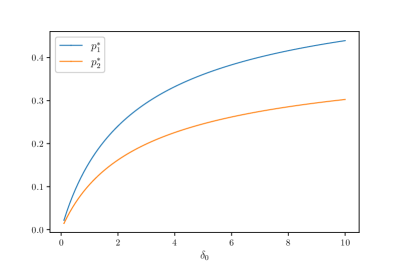
Refer to caption
Figure 2: Impact of δ0subscript𝛿0\delta_{0} on p1superscriptsubscript𝑝1p_{1}^{*} and p2superscriptsubscript𝑝2p_{2}^{*}

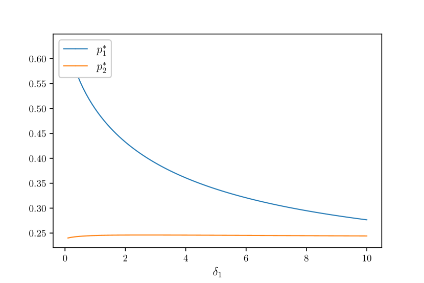
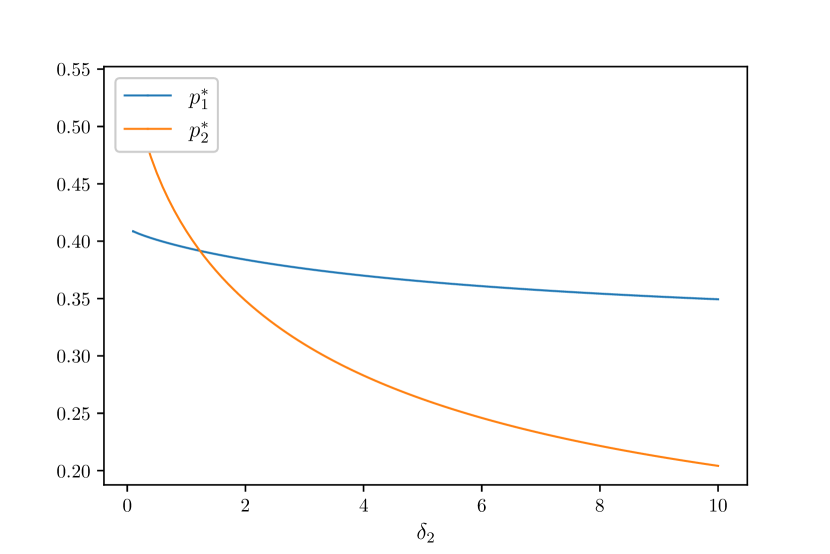
We next study how the risk aversion of the two reinsurers, δ1subscript𝛿1\delta_{1} and δ2subscript𝛿2\delta_{2}, affect the insurer’s decision and plot pisuperscriptsubscript𝑝𝑖p_{i}^{*} as a function of these parameters in Figures 4 and 4, respectively. We observe that, when the risk aversion coefficient of one reinsurer increases, the proportion of reinsurance ceded to this reinsurer will decrease significantly (see the blue curve in Figure 4 and the orange curve in Figure 4); however, the proportion of reinsurance ceded to the other reinsurer may stay almost unchanged (Figure 4) or decrease slightly (Figure 4). The first result can be easily understood as follows. When δisubscript𝛿𝑖\delta_{i} increases, the contract offered by Reinsurer i𝑖i becomes more expensive, and the insurer reacts by ceding less risk to Reinsurer i𝑖i, leading to a decrease of pisuperscriptsubscript𝑝𝑖p_{i}^{*}. However, the impact of δisubscript𝛿𝑖\delta_{i} on pjsuperscriptsubscript𝑝𝑗p_{j}^{*}, ij𝑖𝑗i\neq j, is more subtle because although Reinsurer j𝑗j will raise its premium θjsuperscriptsubscript𝜃𝑗\theta_{j}^{*}, the increase may be at a much slower pace than Reinsurer i𝑖i.

Refer to caption
Figure 3: Impact of δ1subscript𝛿1\delta_{1} on p1superscriptsubscript𝑝1p_{1}^{*} and p2superscriptsubscript𝑝2p_{2}^{*}
Refer to caption
Figure 4: Impact of δ2subscript𝛿2\delta_{2} on p1superscriptsubscript𝑝1p_{1}^{*} and p2superscriptsubscript𝑝2p_{2}^{*}

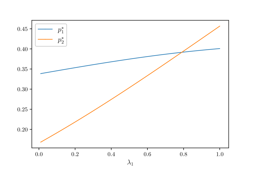
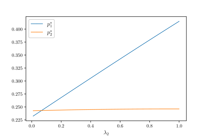
In the last step, we shift our attention to the impact of λ1subscript𝜆1\lambda_{1} and λ2subscript𝜆2\lambda_{2} on the insurer’s equilibrium strategies p1superscriptsubscript𝑝1p_{1}^{*} and p2superscriptsubscript𝑝2p_{2}^{*}. Recall that λisubscript𝜆𝑖\lambda_{i} measures the competition degree of Reinsurer i𝑖i to its competitor Reinsurer j𝑗j in the relative performance (see (2.8)). Both Figures 6 and 6 show that an increase in the competition degree of one reinsurer pushes the insurer to purchase more coverage from both reinsurers, albeit at very different scales. This is because when λisubscript𝜆𝑖\lambda_{i} increases, a more fierce competition drives both reinsurers to lower their premiums, which in turn incentives the insurer to cede more of its risk away to the reinsurers.
Refer to caption
Figure 5: Impact of λ1subscript𝜆1\lambda_{1} on p1superscriptsubscript𝑝1p_{1}^{*} and p2superscriptsubscript𝑝2p_{2}^{*}
Refer to caption
Figure 6: Impact of λ2subscript𝜆2\lambda_{2} on p1superscriptsubscript𝑝1p_{1}^{*} and p2superscriptsubscript𝑝2p_{2}^{*}

4.2 Sensitivity Analysis for the Reinsurers

We next turn our attention to the two reinsurers and investigate how model parameters affect their equilibrium strategies θ1superscriptsubscript𝜃1\theta_{1}^{*} and θ2superscriptsubscript𝜃2\theta_{2}^{*}. Keep in mind that we have already obtained analytical results on the sensitivity of θ1superscriptsubscript𝜃1\theta_{1}^{*} and θ2superscriptsubscript𝜃2\theta_{2}^{*} in Proposition 3.4.

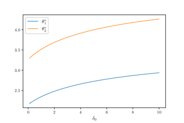
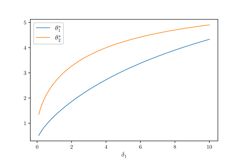
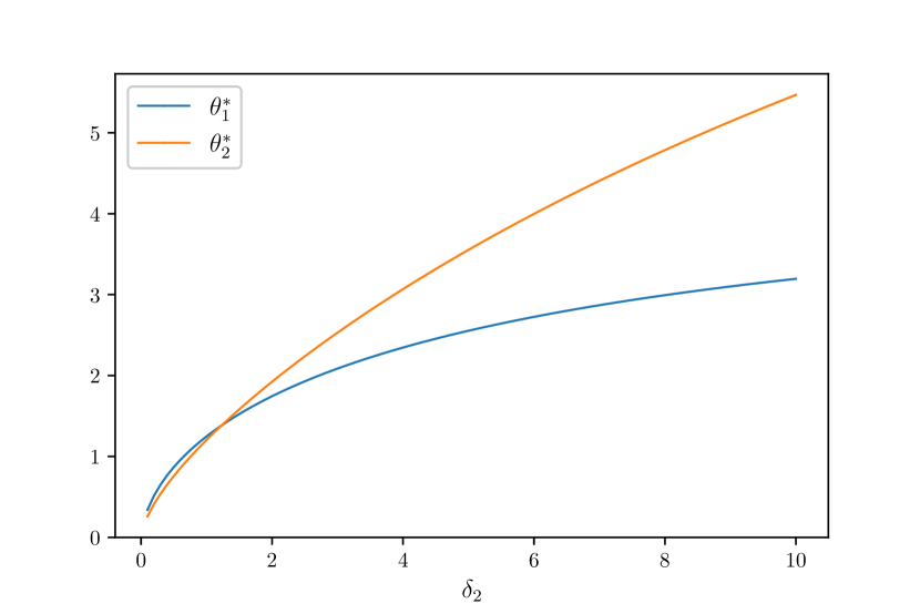
In Figures 7-9, we plot how each reinsurer’s equilibrium premium strategy θisuperscriptsubscript𝜃𝑖\theta_{i}^{*}, i=1,2𝑖12i=1,2, reacts to the change of one player’s risk aversion (δ0subscript𝛿0\delta_{0}, δ1subscript𝛿1\delta_{1}, or δ2subscript𝛿2\delta_{2}). The plots in all figures confirm the positive relation between θisuperscriptsubscript𝜃𝑖\theta_{i}^{*} and δjsubscript𝛿𝑗\delta_{j} established in (3.28). A larger δ0subscript𝛿0\delta_{0} implies a higher demand from the insurer for reinsurance coverage; upon recognizing this, both reinsurers explore such an opportunity by increasing premiums to achieve a higher expected utility. When the risk aversion δisubscript𝛿𝑖\delta_{i} of Reinsurer i𝑖i increases, one naturally anticipates an increase in its own premium θisuperscriptsubscript𝜃𝑖\theta_{i}^{*} because this helps reduce the risk taking by Reinsurer i𝑖i from the insurer. Interestingly, we observe that the increase of δisubscript𝛿𝑖\delta_{i} pushes θjsuperscriptsubscript𝜃𝑗\theta_{j}^{*}, the competitor’s equilibrium premium, up; such a result is likely due to the direct competition implied by the relative performance used in optimization. Last, we observe θ2>θ1superscriptsubscript𝜃2superscriptsubscript𝜃1\theta_{2}^{*}>\theta_{1}^{*} in most scenarios, except for very small δ2subscript𝛿2\delta_{2} in Figure 9. This observation can be explained by the fact that Reinsurer 2 exhibits a higher degree of risk aversion and places a greater emphasis on competition by choosing a larger λ2subscript𝜆2\lambda_{2}.

Refer to caption
Figure 7: Impact of δ0subscript𝛿0\delta_{0} on θ1superscriptsubscript𝜃1\theta_{1}^{*} and θ2superscriptsubscript𝜃2\theta_{2}^{*}
Refer to caption
Figure 8: Impact of δ1subscript𝛿1\delta_{1} on θ1superscriptsubscript𝜃1\theta_{1}^{*} and θ2superscriptsubscript𝜃2\theta_{2}^{*}
Refer to caption
Figure 9: Impact of δ2subscript𝛿2\delta_{2} on θ1superscriptsubscript𝜃1\theta_{1}^{*} and θ2superscriptsubscript𝜃2\theta_{2}^{*}

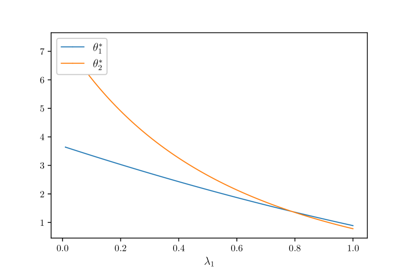
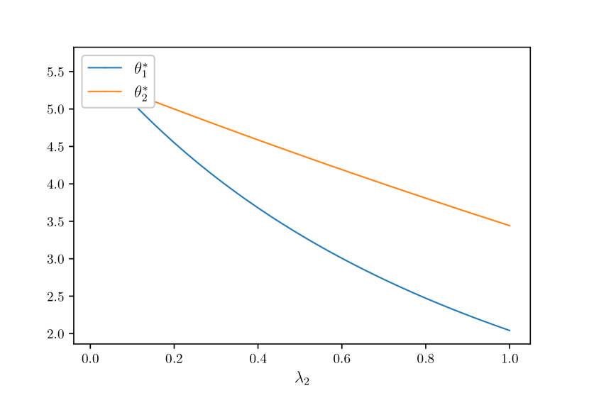
Last, we study the competition degree λisubscript𝜆𝑖\lambda_{i} on the reinsurers’ premium decision. Both Figures 11 and 11 show that when one reinsurer’s competition degree λisubscript𝜆𝑖\lambda_{i} increases, both reinsurers lower their premium loadings. This is due to the “chain effect” of the competition game explained as follows. A larger λisubscript𝜆𝑖\lambda_{i} means that Reinsurer i𝑖i has a stronger incentive to compete with Reinsurer j𝑗j, and to outperform its competitor Reinsurer j𝑗j, Reinsurer i𝑖i’s natural move is to lower its price by choosing a smaller θisuperscriptsubscript𝜃𝑖\theta_{i}^{*}; as Reinsurer j𝑗j also takes into account Reinsurer i𝑖i’s performance in evaluating its utility, it will reduce its loading θjsuperscriptsubscript𝜃𝑗\theta_{j}^{*} in order to stay competitive to Reinsurer i𝑖i.

Refer to caption
Figure 10: Impact of λ1subscript𝜆1\lambda_{1} on θ1superscriptsubscript𝜃1\theta_{1}^{*} and θ2superscriptsubscript𝜃2\theta_{2}^{*}
Refer to caption
Figure 11: Impact of λ2subscript𝜆2\lambda_{2} on θ1superscriptsubscript𝜃1\theta_{1}^{*} and θ2superscriptsubscript𝜃2\theta_{2}^{*}

5 Conclusion

In this paper, we introduce a two-layer stochastic game model to study reinsurance contracting and competition in a market with one insurer and two competing reinsurers. The reinsurance contracting problem between the insurer and each of the two reinsurers is captured by a Stackelberg game, in which the reinsurer is the leader and chooses the loading in its variance premium rule, and the insurer is the follower and chooses its proportional reinsurance strategy. Meanwhile, the competition between the two reinsurers is captured by the fact that each maximizes its expected utility of the relative performance at the terminal time. We solve such a complex game rigorously and completely; we show that a unique equilibrium exists and is fully characterized if 0λ1λ2<10subscript𝜆1subscript𝜆210\leq\lambda_{1}\lambda_{2}<1, and no equilibrium exists if λ1λ21subscript𝜆1subscript𝜆21\lambda_{1}\lambda_{2}\geq 1, in which λi0subscript𝜆𝑖0\lambda_{i}\geq 0 is the competition degree of Reinsurer i𝑖i, i=1,2𝑖12i=1,2. We also obtain several interesting qualitative results of the equilibrium strategies and conduct a numerical study to further study how insurer’s and reinsurers’ risk aversion coefficients, as well as competition parameters, influence the equilibrium strategies.

Acknowledgement.   Zongxia Liang acknowledges the financial support from the National Natural Science Foundation of China (Nos.12271290, 12371477, 11871036). The authors also thank the members of the group of Actuarial Sciences and Mathematical Finance at the Department of Mathematical Sciences, Tsinghua University for their feedback.

Appendix A Technical Results

We first provide a formal verification for the solution to the insurer’s problem obtained in Theorem 3.1. For a similar result, please refer to Fleming and Soner, (2006)[Theorem III.8.1, p.135].

Theorem A.1 (Verification theorem for the insurer’s problem).

Let v0subscript𝑣0v_{0} be a classical solution to the HJB equation (3.7) associated with the insurer’s problem in Definition 2.2. Then, for all (t,x)[0,T]×𝑡𝑥0𝑇(t,x)\in[0,T]\times\mathbb{R} and all θ𝒰1×𝒰2𝜃subscript𝒰1subscript𝒰2\theta\in\mathcal{U}_{1}\times\mathcal{U}_{2}, we have

  • (a)

    v0(x)J0θ(t,x;p)subscript𝑣0𝑥superscriptsubscript𝐽0𝜃𝑡𝑥𝑝v_{0}(x)\geq J_{0}^{\theta}(t,x;p) for every admissible strategy p𝒰0𝑝subscript𝒰0p\in\mathcal{U}_{0}.

  • (b)

    If there exists an admissible p¯𝒰0¯𝑝subscript𝒰0\bar{p}\in\mathcal{U}_{0} such that

    p¯(s)=argminp(s)𝒰0𝒜0(p,θ)v0(s,X¯0(s))¯𝑝𝑠subscriptargmin𝑝𝑠subscript𝒰0superscriptsubscript𝒜0𝑝𝜃subscript𝑣0𝑠subscript¯𝑋0𝑠\displaystyle\bar{p}(s)=\operatorname*{arg\,min}_{p(s)\in\mathcal{U}_{0}}\,\mathcal{A}_{0}^{(p,\theta)}\,v_{0}(s,\bar{X}_{0}(s))

    for almost all s[t,T]𝑠𝑡𝑇s\in[t,T], in which X¯0subscript¯𝑋0\bar{X}_{0} is the insurer’s surplus under p¯¯𝑝\bar{p}, then

    v0(t,x)=V¯0θ(t,x)=J0θ(t,x;p¯).subscript𝑣0𝑡𝑥superscriptsubscript¯𝑉0𝜃𝑡𝑥superscriptsubscript𝐽0𝜃𝑡𝑥¯𝑝\displaystyle v_{0}(t,x)=\bar{V}_{0}^{\theta}(t,x)=J_{0}^{\theta}(t,x;\bar{p}). (A.1)
Proof.

(a) Let v0subscript𝑣0v_{0} be a classical solution to the HJB equation (3.7). For every (p,θ)𝒰𝑝𝜃𝒰(p,\theta)\in\mathcal{U}, applying Itô’s formula to v0(,X0())subscript𝑣0subscript𝑋0v_{0}(\cdot,X_{0}(\cdot)), we get

v0(T,X0(T))subscript𝑣0𝑇subscript𝑋0𝑇\displaystyle v_{0}(T,X_{0}(T)) =v0(t,X0(t))+tT𝒜0(p,θ)v0(s,X0(s))dsabsentsubscript𝑣0𝑡subscript𝑋0𝑡superscriptsubscript𝑡𝑇subscriptsuperscript𝒜𝑝𝜃0subscript𝑣0𝑠subscript𝑋0𝑠differential-d𝑠\displaystyle=v_{0}(t,X_{0}(t))+\int_{t}^{T}\mathcal{A}^{(p,\theta)}_{0}v_{0}(s,X_{0}(s))\,\mathrm{d}s
+tTσ(1p1(s)p2(s))xv0(s,X0(s))dW(s).superscriptsubscript𝑡𝑇𝜎1subscript𝑝1𝑠subscript𝑝2𝑠subscript𝑥subscript𝑣0𝑠subscript𝑋0𝑠d𝑊𝑠\displaystyle\quad+\int_{t}^{T}\sigma(1-p_{1}(s)-p_{2}(s))\partial_{x}v_{0}(s,X_{0}(s))\,\mathrm{d}W(s).

Introduce short-handed notations μ^(t):=cμσ2θ1(t)p12(t)σ2θ2(t)p22(t)assign^𝜇𝑡𝑐𝜇superscript𝜎2subscript𝜃1𝑡superscriptsubscript𝑝12𝑡superscript𝜎2subscript𝜃2𝑡superscriptsubscript𝑝22𝑡\hat{\mu}(t):=c-\mu-\sigma^{2}\theta_{1}(t)p_{1}^{2}(t)-\sigma^{2}\theta_{2}(t)p_{2}^{2}(t) and σ^(t):=σ(1p1(t)p2(t))assign^𝜎𝑡𝜎1subscript𝑝1𝑡subscript𝑝2𝑡\hat{\sigma}(t):=\sigma(1-p_{1}(t)-p_{2}(t)). Recall from Definition 2.1 that both p𝑝p and θ𝜃\theta are uniformly bounded; as such, f0subscript𝑓0f_{0} in (3.4), μ^^𝜇\hat{\mu}, and σ^^𝜎\hat{\sigma} are also uniformly bounded. That is, there exists a positive constant, denoted by M𝑀M, such that

supt[0,T]e2f0(t)M,supt[0,T]|μ^(t)|M,andsupt[0,T]|σ^(t)|M,a.s..formulae-sequencesubscriptsupremum𝑡0𝑇superscripte2subscript𝑓0𝑡𝑀formulae-sequencesubscriptsupremum𝑡0𝑇^𝜇𝑡𝑀andsubscriptsupremum𝑡0𝑇^𝜎𝑡𝑀a.s..\displaystyle\sup_{t\in[0,T]}\mathrm{e}^{2f_{0}(t)}\leq M,\quad\sup_{t\in[0,T]}\left|\hat{\mu}(t)\right|\leq M,\quad\text{and}\quad\sup_{t\in[0,T]}\left|\hat{\sigma}(t)\right|\leq M,\quad\text{a.s..} (A.2)

Then, by a standard localization technique and using (3.7), we obtain

𝔼t,x[v0(T,X0(T))]=v0(t,x)+tT𝔼t,x[𝒜0(p,θ)v0(s,X0(s))]dsv0(t,x)subscript𝔼𝑡𝑥delimited-[]subscript𝑣0𝑇subscript𝑋0𝑇subscript𝑣0𝑡𝑥superscriptsubscript𝑡𝑇subscript𝔼𝑡𝑥delimited-[]subscriptsuperscript𝒜𝑝𝜃0subscript𝑣0𝑠subscript𝑋0𝑠differential-d𝑠subscript𝑣0𝑡𝑥\displaystyle\mathbb{E}_{t,x}\left[v_{0}(T,X_{0}(T))\right]=v_{0}(t,x)+\int_{t}^{T}\mathbb{E}_{t,x}\left[\mathcal{A}^{(p,\theta)}_{0}v_{0}(s,X_{0}(s))\right]\,\mathrm{d}s\leq v_{0}(t,x) (A.3)

and, by the terminal condition in (3.7) and the definition of J0θsuperscriptsubscript𝐽0𝜃J_{0}^{\theta} in (2.6),

𝔼t,x[v0(T,X0(T))]=𝔼t,x[1δ0eδ0X0(T)]=J0θ(t,x;p),subscript𝔼𝑡𝑥delimited-[]subscript𝑣0𝑇subscript𝑋0𝑇subscript𝔼𝑡𝑥delimited-[]1subscript𝛿0superscriptesubscript𝛿0subscript𝑋0𝑇superscriptsubscript𝐽0𝜃𝑡𝑥𝑝\displaystyle\mathbb{E}_{t,x}\left[v_{0}(T,X_{0}(T))\right]=\mathbb{E}_{t,x}\left[-\frac{1}{\delta_{0}}\,\mathrm{e}^{-\delta_{0}X_{0}(T)}\right]=J_{0}^{\theta}(t,x;p),

in which 𝔼t,x:=𝔼[|X0(t)=x]\mathbb{E}_{t,x}:=\mathbb{E}[\cdot|X_{0}(t)=x]. Combining the above two results proves Assertion (a)𝑎(a).

Assertion (b)𝑏(b) is self-evident because the inequality in (A.3) becomes equality when p=p¯𝑝¯𝑝p=\bar{p}. ∎

We now apply Theorem A.1 to verify that the results in Theorem 3.1 hold as claimed.

Verification for Theorem 3.1.

Consider a function v0subscript𝑣0v_{0} given by

v0(t,x)=1δ0eδ0x,(t,x)[0,T]×,formulae-sequencesubscript𝑣0𝑡𝑥1subscript𝛿0superscriptesubscript𝛿0𝑥𝑡𝑥0𝑇\displaystyle v_{0}(t,x)=-\frac{1}{\delta_{0}}\,\mathrm{e}^{-\delta_{0}x},\quad(t,x)\in[0,T]\times\mathbb{R},

in which f0subscript𝑓0f_{0} is defined in (3.4). The proof of Theorem 3.1 shows that v0subscript𝑣0v_{0} is a classical solution in the space of C1,2([0,T]×)superscriptC120𝑇\mathrm{C}^{1,2}([0,T]\times\mathbb{R}) to the HJB equation (3.7), then Assertion (a)𝑎(a) in Theorem A.1 holds. In fact, for such a v0subscript𝑣0v_{0}, the localization technique is not needed because we can directly show that the corresponding Itô process is a martingale. To see that, using (A.2) and setting X0(0)=x0subscript𝑋00subscript𝑥0X_{0}(0)=x_{0}, we obtain

supt[0,T]𝔼[e2δ0X0(t)]=subscriptsupremum𝑡0𝑇𝔼delimited-[]superscripte2subscript𝛿0subscript𝑋0𝑡absent\displaystyle\sup_{t\in[0,T]}\mathbb{E}\left[\mathrm{e}^{-2\delta_{0}X_{0}(t)}\right]= supt[0,T]𝔼[exp(2δ0x02δ00tμ^(s)ds+2δ00tσ^(s)dW(s))]subscriptsupremum𝑡0𝑇𝔼delimited-[]2subscript𝛿0subscript𝑥02subscript𝛿0superscriptsubscript0𝑡^𝜇𝑠differential-d𝑠2subscript𝛿0superscriptsubscript0𝑡^𝜎𝑠differential-d𝑊𝑠\displaystyle\sup_{t\in[0,T]}\mathbb{E}\left[\exp\left(-2\delta_{0}x_{0}-2\delta_{0}\int_{0}^{t}\hat{\mu}(s)\mathrm{d}s+2\delta_{0}\int_{0}^{t}\hat{\sigma}(s)\mathrm{d}W(s)\right)\right]
\displaystyle\leqslant exp(2δ0x0+2δ0MT)supt[0,T]𝔼[exp(2δ00tσ^(s)dW(s))]2subscript𝛿0subscript𝑥02subscript𝛿0𝑀𝑇subscriptsupremum𝑡0𝑇𝔼delimited-[]2subscript𝛿0superscriptsubscript0𝑡^𝜎𝑠differential-d𝑊𝑠\displaystyle\exp\left(-2\delta_{0}x_{0}+2\delta_{0}MT\right)\sup_{t\in[0,T]}\mathbb{E}\left[\exp\left(2\delta_{0}\int_{0}^{t}\hat{\sigma}(s)\mathrm{d}W(s)\right)\right]
\displaystyle\leqslant exp(2δ0x0+2δ0MT+2δ02M2T),2subscript𝛿0subscript𝑥02subscript𝛿0𝑀𝑇2superscriptsubscript𝛿02superscript𝑀2𝑇\displaystyle\exp\left(-2\delta_{0}x_{0}+2\delta_{0}MT+2\delta_{0}^{2}M^{2}T\right),

which in turn implies that

𝔼[0T|σ^(t)xv0(t,X0(t))|2dt]M2supt[0,T]𝔼[e2δ0X0(t)]<.𝔼delimited-[]superscriptsubscript0𝑇superscript^𝜎𝑡subscript𝑥subscript𝑣0𝑡subscript𝑋0𝑡2differential-d𝑡superscript𝑀2subscriptsupremum𝑡0𝑇𝔼delimited-[]superscripte2subscript𝛿0subscript𝑋0𝑡\displaystyle\mathbb{E}\left[\int_{0}^{T}\left|\hat{\sigma}(t)\partial_{x}v_{0}(t,X_{0}(t))\right|^{2}\mathrm{d}t\right]\leqslant M^{2}\sup_{t\in[0,T]}\mathbb{E}\left[\mathrm{e}^{-2\delta_{0}X_{0}(t)}\right]<\infty.

From (3.1) and (3.2), we easily see that

p¯1(t)[0,1],p¯2(t)[0,1],and1p¯1(t)p¯2(t)[0,1],formulae-sequencesubscript¯𝑝1𝑡01formulae-sequencesubscript¯𝑝2𝑡01and1subscript¯𝑝1𝑡subscript¯𝑝2𝑡01\displaystyle\bar{p}_{1}(t)\in[0,1],\quad\bar{p}_{2}(t)\in[0,1],\quad\text{and}\quad 1-\bar{p}_{1}(t)-\bar{p}_{2}(t)\in[0,1],

and p¯=(p¯1,p¯2)=argminp𝒰0𝒜0(p,θ)v0¯𝑝subscript¯𝑝1subscript¯𝑝2subscriptargmin𝑝subscript𝒰0superscriptsubscript𝒜0𝑝𝜃subscript𝑣0\bar{p}=(\bar{p}_{1},\bar{p}_{2})=\operatorname*{arg\,min}_{p\in\mathcal{U}_{0}}\,\mathcal{A}_{0}^{(p,\theta)}\,v_{0}; furthermore, given θ𝒰1×𝒰2𝜃subscript𝒰1subscript𝒰2\theta\in\mathcal{U}_{1}\times\mathcal{U}_{2}, p¯1subscript¯𝑝1\bar{p}_{1} and p¯2subscript¯𝑝2\bar{p}_{2} are progressively measurable. All together proves that p¯𝒰0¯𝑝subscript𝒰0\bar{p}\in\mathcal{U}_{0} is admissible. Therefore, by Theorem A.1, p¯¯𝑝\bar{p} is indeed the insurer’s optimal strategy, and V¯0θ=v0superscriptsubscript¯𝑉0𝜃subscript𝑣0\bar{V}_{0}^{\theta}=v_{0} is the value function. ∎

Proof of Proposition 3.4.

By recalling ΘisubscriptΘ𝑖\Theta_{i} in (3.12), Θi:=Θi(x|δ0,δ1,δ2,λ1,λ2)assignsubscriptΘ𝑖subscriptΘ𝑖conditional𝑥subscript𝛿0subscript𝛿1subscript𝛿2subscript𝜆1subscript𝜆2\Theta_{i}:=\Theta_{i}(x|\delta_{0},\delta_{1},\delta_{2},\lambda_{1},\lambda_{2}) also depends on the parameters δ0,δ1,δ2,λ1,λ2subscript𝛿0subscript𝛿1subscript𝛿2subscript𝜆1subscript𝜆2\delta_{0},\delta_{1},\delta_{2},\lambda_{1},\lambda_{2}. Although previously we have treated ΘisubscriptΘ𝑖\Theta_{i} as a univariate function of x𝑥x in Section 3, we will treat ΘisubscriptΘ𝑖\Theta_{i} as a multivariate function of these parameters in the subsequent sensitivity analysis. As such, Θi(x)superscriptsubscriptΘ𝑖𝑥\Theta_{i}^{\prime}(x) is Section 3 translates to Θi/xsubscriptΘ𝑖𝑥\partial\Theta_{i}/\partial x here.

First, we compute the partial derivatives of ΘisubscriptΘ𝑖\Theta_{i} with respect to each parameter by

Θiδ0subscriptΘ𝑖subscript𝛿0\displaystyle\frac{\partial\Theta_{i}}{\partial\delta_{0}} =2x4(2x2+((1+2λj)δ0+2λjδi)x+λj(1+λj)δ0δi)2>0,absent2superscript𝑥4superscript2superscript𝑥212subscript𝜆𝑗subscript𝛿02subscript𝜆𝑗subscript𝛿𝑖𝑥subscript𝜆𝑗1subscript𝜆𝑗subscript𝛿0subscript𝛿𝑖20\displaystyle=\frac{2x^{4}}{(2x^{2}+((1+2\lambda_{j})\delta_{0}+2\lambda_{j}\delta_{i})x+\lambda_{j}(1+\lambda_{j})\delta_{0}\delta_{i})^{2}}>0, (A.4)
ΘiδisubscriptΘ𝑖subscript𝛿𝑖\displaystyle\frac{\partial\Theta_{i}}{\partial\delta_{i}} =x2(δ0(1+λj)+2x)(2x2+((1+2λj)δ0+2λjδi)x+λj(1+λj)δ0δi)2>0,absentsuperscript𝑥2subscript𝛿01subscript𝜆𝑗2𝑥superscript2superscript𝑥212subscript𝜆𝑗subscript𝛿02subscript𝜆𝑗subscript𝛿𝑖𝑥subscript𝜆𝑗1subscript𝜆𝑗subscript𝛿0subscript𝛿𝑖20\displaystyle=\frac{x^{2}(\delta_{0}(1+\lambda_{j})+2x)}{(2x^{2}+((1+2\lambda_{j})\delta_{0}+2\lambda_{j}\delta_{i})x+\lambda_{j}(1+\lambda_{j})\delta_{0}\delta_{i})^{2}}>0, (A.5)
ΘiδjsubscriptΘ𝑖subscript𝛿𝑗\displaystyle\frac{\partial\Theta_{i}}{\partial\delta_{j}} =0,absent0\displaystyle=0, (A.6)
ΘiλisubscriptΘ𝑖subscript𝜆𝑖\displaystyle\frac{\partial\Theta_{i}}{\partial\lambda_{i}} =0,absent0\displaystyle=0, (A.7)
ΘiλjsubscriptΘ𝑖subscript𝜆𝑗\displaystyle\frac{\partial\Theta_{i}}{\partial\lambda_{j}} =2(δ02+2δ0δi+2δi2)x3+2δ0δi(δ0+2δi)(1+λj)x2+δ02δi2(1+λj)2x(2x2+((1+2λj)δ0+2λjδi)x+λj(1+λj)δ0δi)2<0.absent2superscriptsubscript𝛿022subscript𝛿0subscript𝛿𝑖2superscriptsubscript𝛿𝑖2superscript𝑥32subscript𝛿0subscript𝛿𝑖subscript𝛿02subscript𝛿𝑖1subscript𝜆𝑗superscript𝑥2superscriptsubscript𝛿02superscriptsubscript𝛿𝑖2superscript1subscript𝜆𝑗2𝑥superscript2superscript𝑥212subscript𝜆𝑗subscript𝛿02subscript𝜆𝑗subscript𝛿𝑖𝑥subscript𝜆𝑗1subscript𝜆𝑗subscript𝛿0subscript𝛿𝑖20\displaystyle=-\frac{2(\delta_{0}^{2}+2\delta_{0}\delta_{i}+2\delta_{i}^{2})x^{3}+2\delta_{0}\delta_{i}(\delta_{0}+2\delta_{i})(1+\lambda_{j})x^{2}+\delta_{0}^{2}\delta_{i}^{2}(1+\lambda_{j})^{2}x}{(2x^{2}+((1+2\lambda_{j})\delta_{0}+2\lambda_{j}\delta_{i})x+\lambda_{j}(1+\lambda_{j})\delta_{0}\delta_{i})^{2}}<0. (A.8)

Because θi=Θi(θj)superscriptsubscript𝜃𝑖subscriptΘ𝑖superscriptsubscript𝜃𝑗\theta_{i}^{*}=\Theta_{i}(\theta_{j}^{*}), we have

θiδ0=Θix|x=θjθjδ0+Θiδ0|x=θj.superscriptsubscript𝜃𝑖subscript𝛿0evaluated-atsubscriptΘ𝑖𝑥𝑥superscriptsubscript𝜃𝑗superscriptsubscript𝜃𝑗subscript𝛿0evaluated-atsubscriptΘ𝑖subscript𝛿0𝑥superscriptsubscript𝜃𝑗\displaystyle\frac{\partial\theta_{i}^{*}}{\partial\delta_{0}}=\frac{\partial\Theta_{i}}{\partial x}\Big{|}_{x=\theta_{j}^{*}}\cdot\frac{\partial\theta_{j}^{*}}{\partial\delta_{0}}+\frac{\partial\Theta_{i}}{\partial\delta_{0}}\Big{|}_{x=\theta_{j}^{*}}. (A.9)

Solving the above equations, we get

θiδ0=Θix|x=θjΘjδ0|x=θi+Θiδ0|x=θj1Θix|x=θjΘjx|x=θi>0,superscriptsubscript𝜃𝑖subscript𝛿0evaluated-atevaluated-atsubscriptΘ𝑖𝑥𝑥superscriptsubscript𝜃𝑗subscriptΘ𝑗subscript𝛿0𝑥superscriptsubscript𝜃𝑖evaluated-atsubscriptΘ𝑖subscript𝛿0𝑥superscriptsubscript𝜃𝑗1evaluated-atevaluated-atsubscriptΘ𝑖𝑥𝑥superscriptsubscript𝜃𝑗subscriptΘ𝑗𝑥𝑥superscriptsubscript𝜃𝑖0\displaystyle\frac{\partial\theta_{i}^{*}}{\partial\delta_{0}}=\frac{\frac{\partial\Theta_{i}}{\partial x}\Big{|}_{x=\theta_{j}^{*}}\cdot\frac{\partial\Theta_{j}}{\partial\delta_{0}}\Big{|}_{x=\theta_{i}^{*}}+\frac{\partial\Theta_{i}}{\partial\delta_{0}}\Big{|}_{x=\theta_{j}^{*}}}{1-\frac{\partial\Theta_{i}}{\partial x}\Big{|}_{x=\theta_{j}^{*}}\cdot\frac{\partial\Theta_{j}}{\partial x}\Big{|}_{x=\theta_{i}^{*}}}>0, (A.10)

in which we have used (3.23), (3.26) and (3.27) to derive the inequality

Θix|x=θjΘjx|x=θi<1.evaluated-atevaluated-atsubscriptΘ𝑖𝑥𝑥superscriptsubscript𝜃𝑗subscriptΘ𝑗𝑥𝑥superscriptsubscript𝜃𝑖1\displaystyle\frac{\partial\Theta_{i}}{\partial x}\Big{|}_{x=\theta_{j}^{*}}\cdot\frac{\partial\Theta_{j}}{\partial x}\Big{|}_{x=\theta_{i}^{*}}<1. (A.11)

By following a similar argument, we show the sensitivity results of θisuperscriptsubscript𝜃𝑖\theta_{i}^{*} in (3.28) hold.

Next, we aim to analyze the sensitivity of psuperscript𝑝p^{*} with respect to those model parameters. To that end, recall that pi=p¯i(θ1,θ2)superscriptsubscript𝑝𝑖subscript¯𝑝𝑖superscriptsubscript𝜃1superscriptsubscript𝜃2p_{i}^{*}=\bar{p}_{i}(\theta_{1}^{*},\theta_{2}^{*}), in which p¯1subscript¯𝑝1\bar{p}_{1} and p¯2subscript¯𝑝2\bar{p}_{2} are given by (3.1) and (3.2), respectively. Similar to the above, we now treat each p¯isubscript¯𝑝𝑖\bar{p}_{i} as a function of θ1superscriptsubscript𝜃1\theta_{1}^{*}, θ2superscriptsubscript𝜃2\theta_{2}^{*}, and model parameters, and compute the following derivatives:

p¯iδ0subscript¯𝑝𝑖subscript𝛿0\displaystyle\frac{\partial\bar{p}_{i}}{\partial\delta_{0}} =2θi(θj)2(2θ1θ2+δ0(θ1+θ2))2>0,absent2superscriptsubscript𝜃𝑖superscriptsuperscriptsubscript𝜃𝑗2superscript2superscriptsubscript𝜃1superscriptsubscript𝜃2subscript𝛿0superscriptsubscript𝜃1superscriptsubscript𝜃220\displaystyle=\frac{2\theta_{i}^{*}(\theta_{j}^{*})^{2}}{(2\theta_{1}^{*}\theta_{2}^{*}+\delta_{0}(\theta_{1}^{*}+\theta_{2}^{*}))^{2}}>0, (A.12)
p¯iθisubscript¯𝑝𝑖superscriptsubscript𝜃𝑖\displaystyle\frac{\partial\bar{p}_{i}}{\partial\theta_{i}^{*}} =δ0θj(δ0+2θj)(2θ1θ2+δ0(θ1+θ2))2<0,absentsubscript𝛿0superscriptsubscript𝜃𝑗subscript𝛿02superscriptsubscript𝜃𝑗superscript2superscriptsubscript𝜃1superscriptsubscript𝜃2subscript𝛿0superscriptsubscript𝜃1superscriptsubscript𝜃220\displaystyle=-\frac{\delta_{0}\theta_{j}^{*}(\delta_{0}+2\theta_{j}^{*})}{(2\theta_{1}^{*}\theta_{2}^{*}+\delta_{0}(\theta_{1}^{*}+\theta_{2}^{*}))^{2}}<0, (A.13)
p¯iθjsubscript¯𝑝𝑖superscriptsubscript𝜃𝑗\displaystyle\frac{\partial\bar{p}_{i}}{\partial\theta_{j}^{*}} =δ02θi(2θ1θ2+δ0(θ1+θ2))2>0.absentsuperscriptsubscript𝛿02superscriptsubscript𝜃𝑖superscript2superscriptsubscript𝜃1superscriptsubscript𝜃2subscript𝛿0superscriptsubscript𝜃1superscriptsubscript𝜃220\displaystyle=\frac{\delta_{0}^{2}\theta_{i}^{*}}{(2\theta_{1}^{*}\theta_{2}^{*}+\delta_{0}(\theta_{1}^{*}+\theta_{2}^{*}))^{2}}>0. (A.14)

Let us study the impact of δ0subscript𝛿0\delta_{0} on p1superscriptsubscript𝑝1p_{1}^{*} first and note

p1δ0=p¯1δ0|θ=θ+p¯1θ1|θ=θθ1δ0+p¯1θ2|θ=θθ2δ0,superscriptsubscript𝑝1subscript𝛿0evaluated-atsubscript¯𝑝1subscript𝛿0𝜃superscript𝜃evaluated-atsubscript¯𝑝1superscriptsubscript𝜃1𝜃superscript𝜃superscriptsubscript𝜃1subscript𝛿0evaluated-atsubscript¯𝑝1superscriptsubscript𝜃2𝜃superscript𝜃superscriptsubscript𝜃2subscript𝛿0\displaystyle\frac{\partial p_{1}^{*}}{\partial\delta_{0}}=\frac{\partial\bar{p}_{1}}{\delta_{0}}\Big{|}_{\theta=\theta^{*}}+\frac{\partial\bar{p}_{1}}{\partial\theta_{1}^{*}}\Big{|}_{\theta=\theta^{*}}\cdot\frac{\partial\theta_{1}^{*}}{\partial\delta_{0}}+\frac{\partial\bar{p}_{1}}{\partial\theta_{2}^{*}}\Big{|}_{\theta=\theta^{*}}\cdot\frac{\partial\theta_{2}^{*}}{\partial\delta_{0}}, (A.15)

in which the first and third terms are positive, but the second term is negative. As such, a definite monotonicity result of p1superscriptsubscript𝑝1p_{1}^{*} with respect to δ0subscript𝛿0\delta_{0} is not available in general. By following the same argument, one can see that such a negative result applies to all partial derivatives of pisuperscriptsubscript𝑝𝑖p_{i}^{*}. ∎

References

  • Albrecher et al., (2017) Albrecher, H., Beirlant, J., and Teugels, J. L. (2017). Reinsurance: Actuarial and Statistical Aspects. John Wiley & Sons.
  • Asmussen et al., (2000) Asmussen, S., Højgaard, B., and Taksar, M. (2000). Optimal risk control and dividend distribution policies. Example of excess-of loss reinsurance for an insurance corporation. Finance and Stochastics, 4(3):299–324.
  • Bensoussan et al., (2014) Bensoussan, A., Siu, C. C., Yam, S. C. P., and Yang, H. (2014). A class of non-zero-sum stochastic differential investment and reinsurance games. Automatica, 50(8):2025–2037.
  • Bo et al., (2024) Bo, L., Wang, S., and Zhou, C. (2024). A mean field game approach to optimal investment and risk control for competitive insurers. Insurance: Mathematics and Economics, 116:202–217.
  • Boonen et al., (2021) Boonen, T. J., Tan, K. S., and Zhuang, S. C. (2021). Optimal reinsurance with multiple reinsurers: Competitive pricing and coalition stability. Insurance: Mathematics and Economics, 101(B):302–319.
  • Cai and Chi, (2020) Cai, J. and Chi, Y. (2020). Optimal reinsurance designs based on risk measures: A review. Statistical Theory and Related Fields, 4(1):1–13.
  • Cao et al., (2022) Cao, J., Li, D., Young, V. R., and Zou, B. (2022). Stackelberg differential game for insurance under model ambiguity. Insurance: Mathematics and Economics, 106:128–145.
  • (8) Cao, J., Li, D., Young, V. R., and Zou, B. (2023a). Reinsurance games with n variance-premium reinsurers: From tree to chain. ASTIN Bulletin, 53(3):706–728.
  • (9) Cao, J., Li, D., Young, V. R., and Zou, B. (2023b). Reinsurance games with two reinsurers: Tree versus chain. European Journal of Operational Research, 310(2):928–941.
  • Chen et al., (2016) Chen, L., Qian, L., Shen, Y., and Wang, W. (2016). Constrained investment–reinsurance optimization with regime switching under variance premium principle. Insurance: Mathematics and Economics, 71:253–267.
  • Chen and Shen, (2018) Chen, L. and Shen, Y. (2018). On a new paradigm of optimal reinsurance: A stochastic stackelberg differential game between an insurer and a reinsurer. ASTIN Bulletin, 48(2):905–960.
  • Chen and Shen, (2019) Chen, L. and Shen, Y. (2019). Stochastic Stackelberg differential reinsurance games under time-inconsistent mean–variance framework. Insurance: Mathematics and Economics, 88:120–137.
  • Chi, (2012) Chi, Y. (2012). Optimal reinsurance under variance related premium principles. Insurance: Mathematics and Economics, 51(2):310–321.
  • Fleming and Soner, (2006) Fleming, W. H. and Soner, H. M. (2006). Controlled Markov Processes and Viscosity Solutions. Springer Science & Business Media.
  • Gu et al., (2018) Gu, A., Viens, F. G., and Yao, H. (2018). Optimal robust reinsurance-investment strategies for insurers with mean reversion and mispricing. Insurance: Mathematics and Economics, 80:93–109.
  • Jiang et al., (2019) Jiang, W., Ren, J., Yang, C., and Hong, H. (2019). On optimal reinsurance treaties in cooperative game under heterogeneous beliefs. Insurance: Mathematics and Economics, 85:173–184.
  • Jin et al., (2024) Jin, Z., Xu, Z. Q., and Zou, B. (2024). Optimal moral-hazard-free reinsurance under extended distortion premium principles. SIAM Journal on Control and Optimization, forthcoming.
  • Kroell et al., (2023) Kroell, E., Jaimungal, S., and Pesenti, S. M. (2023). Optimal robust reinsurance with multiple insurers. arXiv preprint arXiv:2308.11828.
  • Li et al., (2015) Li, D., Rong, X., and Zhao, H. (2015). Time-consistent reinsurance–investment strategy for a mean–variance insurer under stochastic interest rate model and inflation risk. Insurance: Mathematics and Economics, 64:28–44.
  • Li and Young, (2022) Li, D. and Young, V. R. (2022). Stackelberg differential game for reinsurance: Mean-variance framework and random horizon. Insurance: Mathematics and Economics, 102:42–45.
  • Liang and Yuen, (2016) Liang, Z. and Yuen, K. C. (2016). Optimal dynamic reinsurance with dependent risks: Variance premium principle. Scandinavian Actuarial Journal, 2016(1):18–36.
  • Lu et al., (2016) Lu, Z., Meng, L., Wang, Y., and Shen, Q. (2016). Optimal reinsurance under VaR and TVaR risk measures in the presence of reinsurer’s risk limit. Insurance: Mathematics and Economics, 68:92–100.
  • Peng et al., (2021) Peng, X., Chen, F., and Wang, W. (2021). Robust optimal investment and reinsurance for an insurer with inside information. Insurance: Mathematics and Economics, 96:15–30.
  • Schmidli, (2001) Schmidli, H. (2001). Optimal proportional reinsurance policies in a dynamic setting. Scandinavian Actuarial Journal, 2001(1):55–68.
  • Schmidli, (2002) Schmidli, H. (2002). On minimizing the ruin probability by investment and reinsurance. Annals of Applied Probability, 12(3):890–907.
  • Tan et al., (2020) Tan, K. S., Wei, P., Wei, W., and Zhuang, S. C. (2020). Optimal dynamic reinsurance policies under a generalized Denneberg’s absolute deviation principle. European Journal of Operational Research, 282(1):345–362.
  • Tan et al., (2009) Tan, K. S., Weng, C., and Zhang, Y. (2009). VaR and CTE criteria for optimal quota-share and stop-loss reinsurance. North American Actuarial Journal, 13(4):459–482.
  • Wang et al., (2020) Wang, G., Wang, Y., and Zhang, S. (2020). An asymmetric information mean-field type linear-quadratic stochastic stackelberg differential game with one leader and two followers. Optimal Control Applications and Methods, 41(4):1001–1370.
  • Yong and Zhou, (2012) Yong, J. and Zhou, X. Y. (2012). Stochastic Controls: Hamiltonian Systems and HJB Equations. Springer Science & Business Media.
  • Zhang and Li, (2021) Zhang, L. and Li, B. (2021). Optimal reinsurance under the α𝛼\alpha-maxmin mean-variance criterion. Insurance: Mathematics and Economics, 101:225–239.
  • Zhou and Yuen, (2012) Zhou, M. and Yuen, K. C. (2012). Optimal reinsurance and dividend for a diffusion model with capital injection: Variance premium principle. Economic Modelling, 29(2):198–207.
  • Zhu et al., (2023) Zhu, M. B., Ghossoub, M., and Boonen, T. J. (2023). Equilibria and efficiency in a reinsurance market. Insurance: Mathematics and Economics, 113:24–49.