Searches for the BSM scenarios at the LHC using decision tree based machine learning algorithms: A comparative study and review of Random Forest, Adaboost, XGboost and LightGBM frameworks

Abstract

Machine learning algorithms are now being extensively used in our daily lives, spanning across diverse industries as well as academia. In the field of high energy physics (HEP), the most common and challenging task is separating a rare signal from a much larger background. The boosted decision tree (BDT) algorithm has been a cornerstone of the high energy physics for analyzing event triggering, particle identification, jet tagging, object reconstruction, event classification, and other related tasks for quite some time. This article presents a comprehensive overview of research conducted by both HEP experimental and phenomenological groups that utilize decision tree algorithms in the context of the Standard Model and Supersymmetry (SUSY). We also summarize the basic concept of machine learning and decision tree algorithm along with the working principle of Random Forest, AdaBoost and two gradient boosting frameworks, such as XGBoost, and LightGBM. Using a case study of electroweakino productions at the high luminosity LHC, we demonstrate how these algorithms lead to improvement in the search sensitivity compared to traditional cut-based methods in both compressed and non-compressed R-parity conserving SUSY scenarios. The effect of different hyperparameters and their optimization, feature importance study using SHapley values are also discussed in detail.

1 Introduction

Supersymmetry (SUSY) Martin:1997ns ; drees2004theory ; baer2006weak is one of the most compelling extensions of beyond the Standard Model (BSM) scenario, and the pursuit of supersymmetric partners of the SM particles (sparticles) remains as a primary objective at the Large Hadron Collider (LHC). Since the inception of the LHC, both the ATLAS and CMS collaborations have already conducted numerous searches to explore the SUSY particles utilizing the LHC Run-I and Run-II dataset atlas_susy ; cms_susy . In the absence of any statistical deviations from the SM predictions, the LHC has set stringent lower bounds on the masses of particles. For example, in the R-parity conserving (RPC) SUSY scenarios with relatively light neutralinos ($\widetilde{\chi}_{1}^{0}$), the LHC Run-II data has extended the lower bounds on the masses of gluino ($m_{\widetilde{g}}$), first two generations light squarks ($m_{\widetilde{q}}$), the lightest stop ($m_{\widetilde{t_{1}}}$) and the lightest chargino ($m_{\widetilde{\chi}_{1}^{\pm}}$) upto $\sim$ 2.3 TeV, 1.6 TeV, 1.2 TeV and 1.2 TeV respectively atlas_susy ; cms_susy depending on the branching ratios and the simplified models assumptions.

It is important to note that the accumulated luminosity of Run-II data is approximately $\sim$ 140 $\rm{fb}^{-1}$, which is about 5% of the luminosity of planned upgrade of high luminosity LHC (HL-LHC) run ($\mathcal{L}=3000\rm{fb}^{-1}$). The LHC Collaboration initiated the Run-III operation in July 2022, and it will continue the operation until the planned three-year-long shutdown (LS3) in preparation for the high luminosity upgrade, which is scheduled to commence in 2026. The constraints on sparticle masses, derived from LHC Run-I and Run-II data, are primarily derived within the framework of simplified SUSY scenarios, which involve specific assumptions regarding decay modes, branching ratios, etc. Also, the majority of the analyses have concentrated on prompt decay scenarios. However, there are several pockets of SUSY parameter spaces with light sparticles that remain less explored, e.g., quasi-degenerate SUSY scenarios where the next to LSP (NLSP) - LSP mass gap is very small Bhattacherjee:2013wna ; Dutta:2015exw ; Chakraborti:2017dpu ; Chowdhury:2016qnz ; Dutta:2017jpe . Such compressed SUSY models are also highly motivated in the context of Dark Matter (DM) relic density KumarBarman:2020ylm ; Barman:2022jdg ; He:2023lgi ; Chakraborti:2015mra ; Chakraborti:2014gea ; Chakraborti:2017dpu ; Chowdhury:2016qnz ; Bhattacharyya:2011se ; Choudhury:2012tc ; Baer:2021aax , Muon (g-2) anomaly Chakraborti:2022vds ; He:2023lgi ; Chakraborti:2015mra ; Chakraborti:2014gea ; Baer:2021aax ; Athron:2021iuf ; Endo:2021zal ; Chakraborti:2021bmv ; Choudhury:2017acn ; Choudhury:2017fuu ; Banerjee:2018eaf ; Banerjee:2020zvi ; Chakraborti:2021dli ; Frank:2021nkq ; Ali:2021kxa ; Kowalska:2015zja ; Chakrabortty:2015ika ; Choudhury:2016lku . It has been observed that conventional cut and count analyses are highly competitive for non-degenerate SUSY searches compared to machine learning (ML) analyses. But ML based analyses give better sensitivity in both degenerate and non-degenerate BSM physics searches.

The term “machine learning” (ML) was first proposed by A. Samuel in 1959 Samuel1988 . After six decades, ML algorithms are now being widely used in our daily lives and across various industries, e.g., filtering email, social media recommendation, cyber security, image analysis and disease detection in healthcare, data analysis in the finance sector, autonomous vehicles, marketing and advertising, etc. In the future, the applications of ML will continue to expand rapidly with the advancement of technology and the availability of more data. high energy physics (HEP) experimental and phenomenological analyses deal with large amount of data and it has been observed that the use of ML techniques leads to improvements in the data analyses of several HEP fields. For particle identification, event selection, object reconstruction, event classification, etc., the experimental high energy physics (HEP-Ex) collaborations have been using the conventional ML algorithms for more than three decades. boosted decision tree (BDT) is one of the most popular algorithms which has been widely used by the HEP-Ex collaborations e.g., the search of single top quark prediction by the CDF and D0 collaborations CDF:2010eor ; D0:2008wma ; D0:2006ngk , Higgs discovery at the LHC CMS:2014afl . For a long time, the HEP community has used BDT and other algorithms implemented in the Toolkit for Multivariate Data Analysis (TMVA) software package TMVA:2007ngy while XGBoost (Extreme Gradient Boosting) has gained immense popularity in recent years Chen:2016btl . However, it should be noted that the deep neural networks (DNN) or deep learning (DL) techniques, which are based on multilayer NN, are becoming more popular nowadays doi:10.1142/S0217751X20020030 ; dnn ; Bhat:2010zz ; Guest:2018yhq ; Bourilkov:2019yoi ; Schwartz:2021ftp ; Carleo:2019ptp ; Shlomi:2020gdn ; Abdughani:2019wuv . There are several broad reviews in the literature on the applications of BDT Bhat:2010zz ; Cornell:2021gut ; Coadou:2022nsh , deep learning algorithm doi:10.1142/S0217751X20020030 ; dnn ; Bhat:2010zz ; Guest:2018yhq ; Bourilkov:2019yoi ; Schwartz:2021ftp ; Carleo:2019ptp ; Shlomi:2020gdn ; Abdughani:2019wuv like convolutional neural networks (CNN), recurrent neural networks (RNN) etc. in the context of high energy physics.

The collider analyses in HEP typically involve with searches of new physics signals and the precise measurements of the existing known SM processes. To achieve this, one has to look for faint signal from a large amount of background where the distribution of signal and backgrounds have significant overlap. Traditional cut-based analysis shows less sensitivity for significant overlap scenarios. In such cases, the ML algorithms are more powerful in discriminating signals from backgrounds. In this article, we will focus on the various kinds of decision tree (DT) based algorithms and study how these algorithms lead to improvement in the search sensitivity compared to cut-based methods considering a case study of electroweakino pair production at the HL-LHC. The structure of the article is as follows. In Sec. 2, we introduce the basic concepts of machine learning along with different kinds of metrics. In Sec. 3, we briefly summarize the major important analyses involving the use of ML algorithms with an emphasis on DT-based algorithms. The basic concepts of decision trees are discussed in Sec. 4. Also, we present a concise overview of Random Forest, AdaBoost, and extreme gradient boosting algorithms such as XGBoost and LightGBM in this section. In Sec. 5, we investigate the improvement of search sensitivity by these four ML algorithms with comparison to cut-and-count analysis using a SUSY scenario with $\widetilde{\chi}_{1}^{\pm}\widetilde{\chi}_{2}^{0}$ (wino-like) pair production. We also present the role of hyperparameters in different ML framework along with the feature importance study using SHapley values. Finally, we summarize the paper in Sec. 6.

2 Basic concepts of machine learning

Machine learning, as a subset of artificial intelligence (AI), involves the development of various models that can learn from diverse datasets and execute tasks without requiring explicit programming. To perform a machine learning (ML) analysis, it is essential to collect data, which comprises information about the desired output that we want the computer to learn. The ML algorithms can be broadly categorized into supervised and unsupervised learning inbook ; hastie2009elements ; carbonell1983overview . In addition to these two, there is also a third category known as semi-supervised learning. In supervised learning, each input data point ($x_{i}$, i = 1,….n, for n input data samples) is accompanied by a target variable or output label ($y_{i}$) and the algorithm learns to extrapolate patterns from the provided training data in order to predict the output labels for unseen (testing) data points. In other words, the aim of the supervised learning is to acquire a mapping function $f$ from the input data to output label: $f:x_{i}\rightarrow y_{i}$ such that it can accurately predict $y_{i}$ for a new data sets (testing) which do not have output labels.

Supervised learning algorithms like decision trees (DT), support vector machines (SVM), logistic regression (LR), neural networks (NN), etc, are commonly used for two major tasks: classification and regression. In the classification task, the output/target is discrete, categorical, and finite, while the output is continuous and infinite for the regression task. For the HEP problems, the simplest example of binary classification is the categorization of the signal and backgrounds for the sensitivity study and one example of a regression task is object tagging. In this paper, we will concentrate on supervised DT algorithms. On the other hand, for the unsupervised learning algorithms (e.g., k-means clustering, autoencoders, etc.) the data only contains input features without any target output variables/values and the algorithms explore the hidden structures or patterns to perform tasks like clustering, anomaly detection, etc. For a recent review of unsupervised machine learning in the context of particle physics, see Ref. Bardhan:2024zla .

In high energy physics (HEP), each and every particle of an event has different four-momentum information along with different energy depositions in the detector. These attributes serve as the basis for constructing different input features for analysis so that the ML algorithm can distinguish the signal and background efficiently. The available dataset is commonly divided into two subsets: training data and testing data. The training data is used to train the model, while the testing data is used to assess the model’s performance on unseen data. Sometimes, we use another set of independent data, known as validation data, to fine-tune the hyperparameters, such as learning rate, regularization strength, or the number of layers in a neural network, etc.

Figure 1: Schematics to demonstrate optimization of mean squared error as a loss function ($L^{MSE}$). The data points are denoted as orange circles, and the prediction is denoted by the red line. The length of the blue dotted lines signifies the difference between the actual value and the predicted value. Left and right models correspond to high and low loss, respectively.

2.1 Loss Function

In supervised learning, the ML algorithm learns using a loss function. Using optimization techniques like Gradient Descent, the loss function is minimized during training by adjusting parameters, which are known as “weights”. For example, the predicted output $y$ in a linear regression model is calculated as $y=f(x_{i})=w_{i}.x_{i}+b$, where b is the bias term. For decision trees, weights may indicate how much each feature contributes to the decision at each node of the tree. The minimization of the loss function specified that the model predicted values are close to the actual value/label. For different types of tasks or data, the choices of loss function vary. The commonly used function for regression tasks is the mean squared error (MSE) and is defined as hastie2009elements ; article ; bentejac2021comparative

$$L^{MSE}=\frac{1}{n}\sum_{i=1}^{n}(\hat{y_{i}}-f(x_{i}))^{2}=\frac{1}{n}\sum_{i=1}^{n}(\hat{y_{i}}-y_{i})^{2}$$ (1)

where $n$ is the number of samples in the dataset, $y_{i}$ and $\hat{y_{i}}$ are the predicted and true target value of the $i^{th}$ sample. Another common loss function for regression tasks is mean absolute error and is defined as

$$L^{MAE}=\frac{1}{n}\sum_{i=1}^{n}|\hat{y_{i}}-y_{i}|$$ (2)

For binary classification tasks the commonly used the most commonly used function is Binary Cross-Entropy Loss or Log Loss, which is defined as:

$$L^{BCE}=-\{\hat{y_{i}}\mathrm{log}(y_{i})+(1-\hat{y_{i}})(\mathrm{log}(1-y_{i}))\}$$ (3)

where $y_{i}$ is the predicted probability and $\hat{y_{i}}$ is the true binary label (0 or 1). Categorical cross-entropy loss ($\sum_{i=1}^{n}\hat{y_{i}}$ log(y)) is used in multi-class classification tasks.

2.2 Overfitting and underfitting

After training the dataset and adjusting the “hyperparameters”, one proceeds to assess the model’s ability to generalize or to make accurate predictions for unseen testing data. However, the complexity of the trained model and the amount of training data can lead to two major issues: overfitting and underfitting.

Figure 2: A sample diagram to illustrate underfitting (high bias, low variance), overfitting (low bias, high variance) and good fitting (low bias, low variance) for a training dataset with signal (magenta points) and backgrounds (cyan points).

$Overfitting$ arises when a model becomes too complex and learns the training data too precisely. Then, the model captures noise in the data instead of the underlying patterns. As a result, the loss computed for the training data tends to approach zero, while it becomes significantly higher for unseen or new testing data. This lack of generalization leads to poor performance on the testing data. Bias represents the deviation of the predicted value from the actual value, while variance indicates the model’s sensitivity to small fluctuations in the training data. Therefore, an overfitted model typically exhibits low bias and high variance. Conversely, if the model is too simple and fails to capture the underlying patterns in the training data, it performs poorly on both the training and testing data. This high bias and low variance scenario is known as underfitting. A good/robust model is a trade of both the parameters - bias and variance. In other words, the right balance between model complexity and the amount of training data is essential for building models that generalize well to unseen data. In Fig. 2 we demonstrate an example of underfitting, overfitting and appropriate fitting by considering a dataset consisting of signal (circular magenta points) and background events (square cyan points). In the left panel, the model is too simple, underfitted, and has a very high bias. On the other hand, the lowest loss is obtained for the middle panel. However, the prediction of this overfitted model is not reliable for the new dataset. The right panel of Fig. 2 represents a robust model that predicts accurately for untrained data.

		Predicted class
		Signal	Background
Class	Signal	True Positive (TP)	False Negative (FN)
True	Background	False Positive (FP)	True Negative (TN)

Table 1: Graphical representation of confusion matrix for binary classification in a typical HEP event analysis.

2.3 Measures of classification performance

After training, tuning of hyperparameter and testing the HEP data, our objective is to evaluate the effectiveness and accuracy of the machine learning models in solving a specific task, e.g., classify or distinguish between signal and background events despite their similar signature. Performance metrics are quantitative indicators used to measure the model’s ability to make accurate predictions or classifications. By evaluating performance metrics, we can compare different ML models and optimize the hyperparameter tuning to improve the model’s effectiveness. Sometimes, the highly skewed distribution of classes in the dataset leads to class imbalance, which affects the performance of the ML algorithm. Techniques like oversampling of the minority class or undersampling of the majority class, adjustment of class weights, cost-effective learning, etc., can be employed to address the class imbalance in ML Cornell:2021gut ; weiss2003learning ; Chawla2005 ; sulaiman ; satio ; LUQUE2019216 ; 10.1007/978-3-642-04962-0_53 . To evaluate the performance metrics, the algorithm checks the actual and predicted values of observations in the dataset by forming confusion matrix. When the signal/background events are correctly classified as signal/background events, then those events are called True Positive (TP) or True Negative (TN). On the other hand, False Positive (FP), False Negative (FN) are the number of events where the actual background/signal events are incorrectly classified as signal/background events. In the Table. 1, we present the confusion matrix graphically for binary classification. With these definitions, we can define the following various performance metrics to evaluate the performance of the model:

• Sensitivity or Recall or True Positive Rate (TPR): Recall, also known as sensitivity or TPR, is defined as the ratio of the number of true positives (correctly predicted signal events) to the total number of actual positives/signal events (TP + FN). Sensitivity is useful for minimizing the occurrence of false negatives.

  $$\textrm{Recall~{} =~{}TPR }=\frac{TP}{TP+FN}$$ (4)

• Precision: Precision measures how many of the events predicted as signal events are actually signals. It is useful when the purpose is to limit the number of false positives or incorrectly classified signal events.

  $$\textrm{Precision~{} }=\frac{TP}{TP+FP}$$ (5)

• Accuracy: Accuracy measures the overall correctness and is defined as the ratio of correct predictions to the total no of events/samples.

  $$\textrm{Accuracy~{} }=\frac{TP+TN}{TP+TN+FP+FN}$$ (6)

• Specificity or True Negative Rate (TNR): Specificity is the ratio of true background to the total number of background events.

  $$\textrm{Specificity~{} }=\frac{TN}{TN+FP}$$ (7)

• ROC curve and area under the curve (auc): The ROC (Receiver Operating Characteristic) curve is a graphical representation of TPR or recall against FPR or (1 - specificity) for various threshold settings. In HEP, the ROC curve relates the signal efficiency versus background efficiency/rejection plane as shown in Fig 24 and the curve illustrates the ability of a binary classifier to separate signal and background events. The ROC curve ends at (1,1) for a perfect classifier that accepts 100% signal events and rejects 100% background events. The area under the ROC curve is known as auc metric and it varies from 0 to 1. For a perfect classifier, the auc becomes one and random guessing leads to auc value = 0.5. Thus the auc metric is a powerful tool for the evaluation of the overall ranking performance of a binary classifier sulaiman .

• F-score metric: F-score is a measure that combines recall and Precision, and it is basically the harmonic mean of them. F-score can be tuned via a real parameter ($\beta$) and the generic expression is given by:

  $$F_{\beta}=(1+\beta^{2})\frac{precision\times recall}{(\beta^{2}\times precision)+recall}$$ (8)

  For $\beta=1$, it is known as $F_{1}$-score metric and expressed as $(2\times precision\times recall)/(precision+recall)$. The F-score can be a better measure than the accuracy metric on imbalanced datasets. A high recall and precision rates indicate low FN and low FP rates and $F_{1}$ score can be useful for imbalanced HEP dataset where the signal events are very rare compared to backgrounds.

• Approximate Median Significance (ams) score: In the field of high energy physics, the primary goal is to optimize the discovery significance. To estimate the discovery significance, the formulas $s/\sqrt{b}$ or $s/\sqrt{(s+b)}$ are commonly used, where s and b denote the numbers of signal and background events, respectively, that remain after the signal selection cuts. It may be noted that in a typical Poisson counting experiment, where $n$ events are observed, the Poisson distribution often features a large mean value, $(s+b)$. However, the formula $s/\sqrt{b}$ is valid only for $b>>s$ and it overestimates the discovery significance when the background events are small Cowan2012DiscoverySF ; Cowan:2010js . For a Poisson counting experiment with negligible uncertainty, the Asimov approximation for the median significance (ams score) is given by Cowan2012DiscoverySF ; Cowan:2010js :

  $$\textrm{significance~{}(ams)}=\sqrt{2\left((s+b)\times ln(1+\frac{s}{b})-s\right)}$$ (9)

  For the scenarios with very small background events, $b$ is replaced by $(b+b_{r})$, where $b_{r}$ is a regularization term typically set to stabilize the calculation. Expanding the logarithm in s/b, the Eq.9 reduces to $\frac{s}{\sqrt{b}}(1+\mathcal{O}(s/b))$. In the context of particle physics experiments, there is generally an uncertainty with the background and this uncertainty ($\Delta$) reduces the significance or the ams score. Due to the presence of the uncertainty, the Eq.9 modifies as Cowan2012DiscoverySF

  $$ams=\sqrt{2\left((s+b)~{}ln\left(\frac{(s+b)(b+\Delta^{2}b^{2})}{b^{2}+(s+b)\Delta^{2}b^{2}}\right)-\frac{1}{\Delta^{2}}~{}ln\left(1+\frac{\Delta^{2}b^{2}s}{b(b+\Delta^{2}b^{2})}\right)\right)}$$ (10)

3 Machine learning in High Energy Physics

In this section, we primarily review the studies that have utilized decision tree-based algorithms within the context of Standard Model (SM) and Beyond Standard Model (BSM) physics scenarios. A comprehensive list of references, grouped into a minimal number of topics, is regularly updated in the Living Review (hepmllivingreview, ), covering various categories like ML review works, classification and regression in supervised or unsupervised learning, generative models and more.

Figure 3: AdaBoost output distributions for signal and background events used in MiniBoone experiment (adapted from Ref ROE2005577 ).

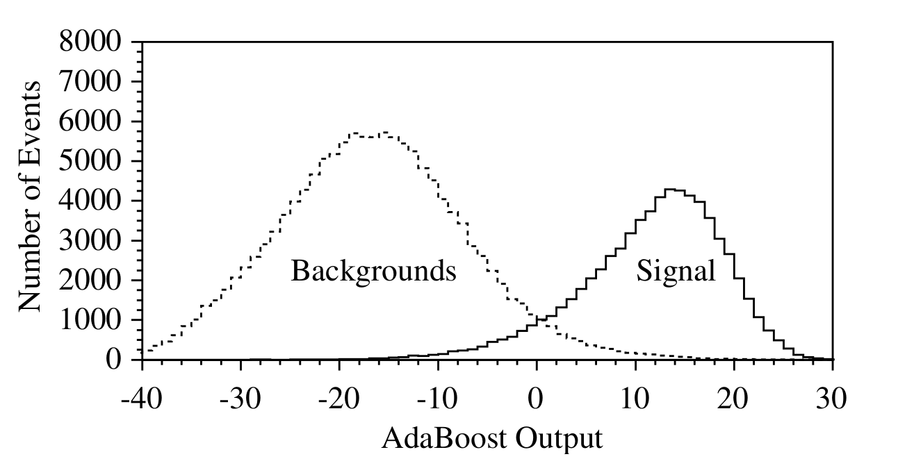
Nearly two decades ago, the first notable use of a boosting algorithm and its performance comparison with the artificial neural network (ANN) and other algorithms was made in the MiniBooNE experiment at Fermilab, which was designed to explore neutrino oscillations ROE2005577 ; YANG2005370 . It was observed that particle identification (PID) with AdaBoost FREUND1997119 algorithm is better than the standard ANN PID technique or Random Forest ROE2005577 ; YANG2005370 . The separation between signal and background events from AdaBoost algorithms is shown in Fig.3 where the choice of parameters was: $\beta$ = 0.5, the number of trees ($N_{tree}$) = 1000 and the number of leaves ($N_{leaves}$) = 45. In the next few years, D$\cancel{0}$ and CDF experiments at Fermilab used the BDT algorithm along with other algorithms like neural network, matrix elements, etc. for the analyses of single top quark production from the Tevatron data D0:2006ngk ; D0:2008wma ; CDF:2010eor . The performance of the BDT algorithm was slightly better than others and the combined results of different techniques led to the initial evidence and subsequent observation of single top quark production D0:2006ngk ; D0:2008wma ; CDF:2010eor . The importance of BDT analysis for this observation has been discussed in a recent review Coadou:2022nsh . Over the past twenty years, the HEP community has been applying the BDT and other more advanced algorithms extensively for event triggering, event generation, parameter space exclusion/scan, jet identification/tagging, event classification and more.

Event Triggering: In particle physics experiments, the event triggering is very crucial for managing the enormous volume of data, reducing the event rates for storage, conducting real-time analyses, enhancing the sensitivity of new physics searches, etc. The CMS collaboration has implemented BDT in the Endcap Muon Track Finder (EMTF) at the Level 1 (L1) trigger level for the LHC Run-II data collection CMS:2018wav . Also, after Phase-2 upgrade, the CMS experiment will use a dedicated BDT classifier at the HGCAL to achieve optimal signal efficiency while rejecting pileup-induced backgrounds Zabi:2020gjd . The high-level trigger (HLT) algorithms run in an online environment and they must be very fast. The LHCb collaboration has reoptimized the HLT using a bonsai BDT (BBDT) algorithm Gligorov:2012qt within the Adaboost framework Likhomanenko:2015aba . It may be noted that for exotic events with long-lived particles (LLPs) searches, the existing triggers are not suitable enough to select the displaced events at the HL-LHC. In such cases, modern machine learning algorithms like lightweight graph autoencoder can be more promising Bhattacherjee:2023evs .

Event Simulation and Parameter space scanning: Monte Carlo event generations, along with fast detector simulations, are becoming more and more computationally expensive as the size of the LHC data is increasing. Also, for the generation of events with multiple outgoing particles or the simulations of next-to-leading (NLO) order processes with a large number of additional jets at the LHC/HL-LHC, the evaluation of matrix elements becomes computationally intensive. A new machine learning algorithm based on gradient BDT (GBDT) has been proposed and tested for Monte Carlo integration in Ref. Bendavid:2017zhk . Most commonly, the exploration of the parameter space of a new physics model involves the evaluation of some complex likelihood function. Using popular approaches like frequentist and Bayesian statistics coupled with Markov Chain Monte Carlo (MCMC) methodology or MultiNest Feroz:2007kg ; Feroz:2008xx ; Trotta:2008bp algorithm based on Nested Sampling 10.1111/j.1365-2966.2009.14548.x , several phenomenological groups have analyzed and constrained the SUSY parameter space Trotta:2008bp ; GAMBIT:2017snp ; GAMBIT:2017zdo ; Choudhury:2023lbp . A recent study has explored the effectiveness of Random Forest (RF) classifier, which is a decision tree based algorithm, in accurately predicting whether a particular SUSY model is excluded by LHC data or not Caron:2016hib . For the Monte Carlo simulation and scanning or recasting of SUSY parameter space, the HEP community has also extensively used more modern/advanced machine learning techniques like Multilayer Perceptron (MLP) Bridges:2010de ; Buckley:2011kc Bayesian Neural Network (BNN) Kronheim:2020vct , Graph Neural Network Mullin:2019mmh , Generative Adversarial Network (GAN) DiSipio:2019imz ; Butter:2019cae ; Lin:2019htn ; Musella:2018rdi , active learning (AL) Ren:2017ymm ; Caron:2019xkx etc. These studies showed that the use of ML algorithms reduces CPU time and storage. For a recent review on the sampling of BSM parameter spaces subjected to available experimental data using machine learning algorithms, please see Ref. Baruah:2024gwy .

Figure 4: The performance comparison (signal efficiency vs background rejection characterized in the form of a ROC curve) of the $W$-boson (left) and top-quark taggers are shown here as obtained by the ATLAS Collaboration ATLAS:2018wis using LHC Run-II data with $\mathcal{L}=36\rm{fb}^{-1}$. The performance of BDT and DNN algorithms is quite similar.

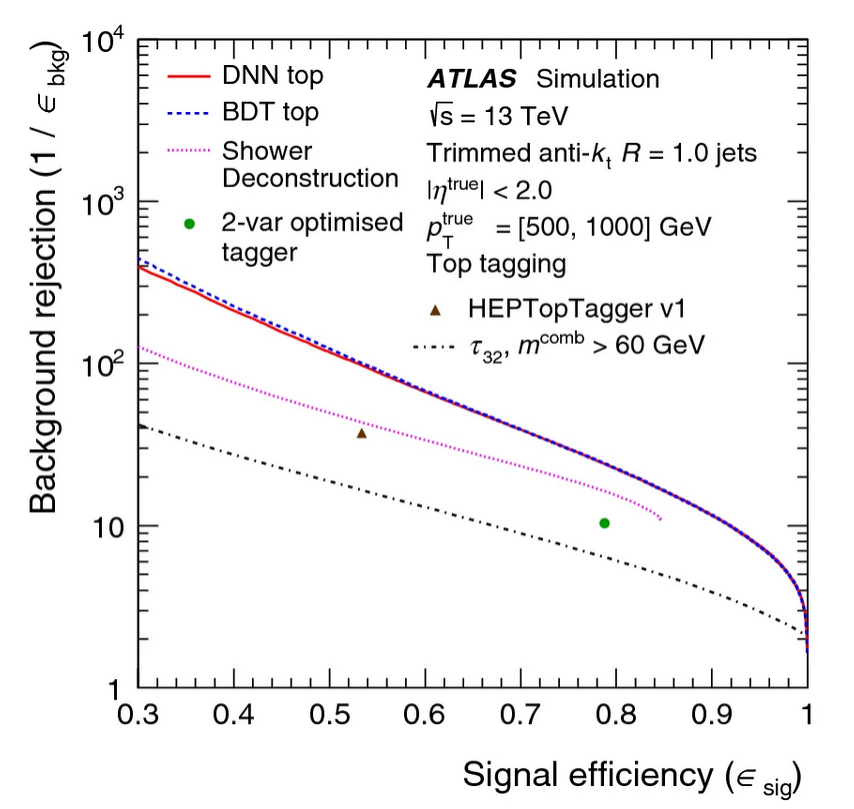
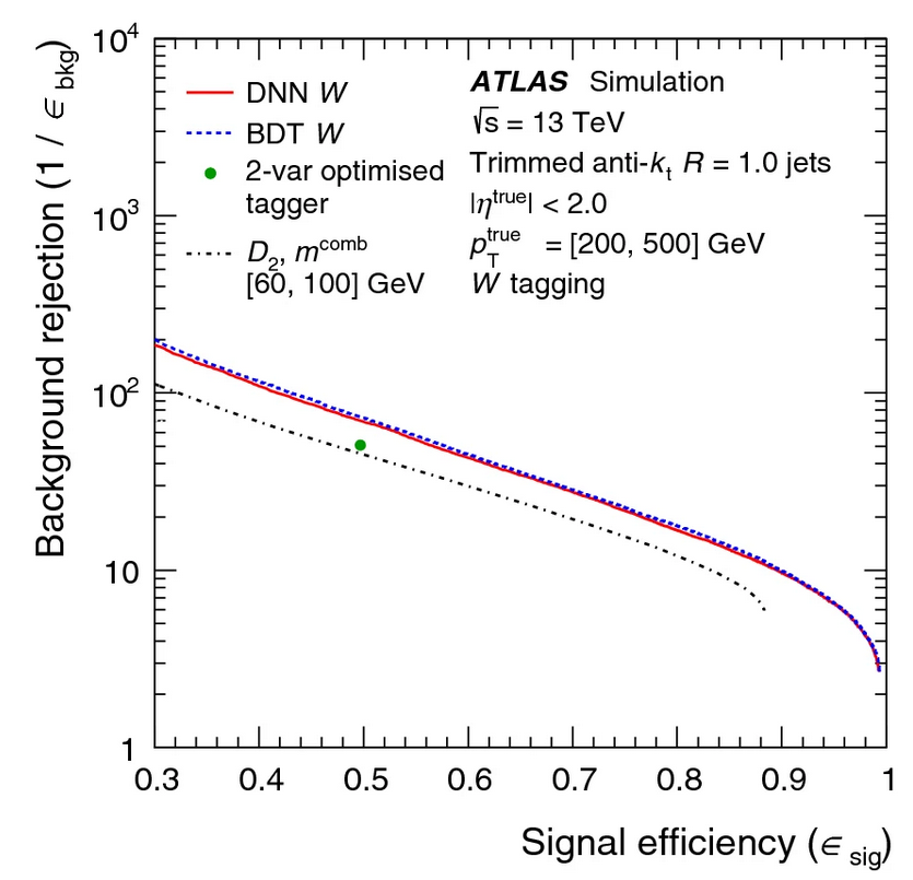
Jet tagging: In collider experiments, the reconstruction and identification of hadronic jets are integral components for physics analyses. Jets originating from massive particles (e.g., bottom quark, top quark, $W/Z/h$ bosons or supersymmetric partner of top quark ($m_{\widetilde{t_{1}}}$)) are usually boosted and collinear. Jets emerging from b-quark are associated with long lifetime and secondary vertex and can be differentiated from other jets coming from light quarks. Motivated by computer vision techniques, jet images was first introduced in Ref. Cogan:2014oua and then many groups have used modern deep neural network (DNN) architectures for jet tagging with jet images deOliveira:2015xxd ; Baldi:2016fql ; Komiske:2016rsd ; Chakraborty:2019imr ; ATLAS:2017dfg . The CMS collaboration has developed DeepCSV CMS:2017wtu ; Bols:2020bkb , DeepFlavour  2020HeavyFI ; deepflv and DeepJet Bols:2020bkb taggers for multiclass classification for light jets, gluon jets, c-jets and b-jets using a deep learning algorithm. In a recent work ATLAS:2019bwq , the ATLAS Collaboration has developed two high-level b-tagging algorithms - MV2 and DL1 Krizhevsky2012ImageNetCW . MV2 Krizhevsky2012ImageNetCW algorithm is based on BDT and is trained within the TMVA framework TMVA:2007ngy . The performance of b-jets tagging using the simulated $t\bar{t}$ events has been presented in Fig.1 in ATLAS:2019bwq for BDT and deep feed-forward neural network algorithms. Although for jet images, tagging, and substructure studies, deep learning algorithms are the most efficient ones, the ATLAS collaboration recently showed that W-boson tagging and top quark tagging ML algorithms lead to a significant gain in efficiency compared to cut-based analysis, as presented in Fig.4 ATLAS:2018wis . This analysis has been performed using LHC Run-II data with $\mathcal{L}=36\rm{fb}^{-1}$. It may be noted that both the BDT and DNN-based algorithms perform similarly to each other for all signal efficiencies ATLAS:2018wis .

3.1 Signal and background events classification

As mentioned earlier, the most important goal of a collider experiment is the production and search of new particles by identifying rare (mostly) signal events from huge backgrounds. The last missing piece of the Standard Model, aka the Higgs boson, was discovered by the CMS and ATLAS collaboration in 2012 ATLAS:2012yve ; CMS:2012qbp . The CMS Collaboration has used the BDT algorithm, implemented within the TMVA framework TMVA:2007ngy , for the Higgs discovery analysis in Ref CMS:2012qbp . Using the full dataset collected in 2011 and 2012 from 7 & 8 TeV LHC run, CMS has updated the $h\to\gamma\gamma$ analysis in Ref. CMS:2014afl , where BDT has been used extensively for several tasks such as - photon identification, photon vertex reconstruction, signal-background classification with good diphoton mass resolution, classification of VBF, Vh, $t\bar{t}h$ tagged events etc. ATLAS Collaboration has also performed an analysis of $t\bar{t}h$ production, where the Higgs boson (h) decays to a $b\bar{b}$ pair, using Run-II data with $\mathcal{L}=36.1\rm{fb}^{-1}$ ATLAS:2017fak . In this analysis Classification BDT has been trained to separate the signal ($t\bar{t}h$ ) from backgrounds and ATLAS has used Reconstruction BDT to select the best combination of jet-parton to reconstruct the Higgs boson and top quark candidates ATLAS:2017fak . In the next subsection, we will summarize the R-parity conserving (RPC) and R-parity violating (RPV) Barbier:2004ez ; Choudhury:2024ggy searches using DT/BDT-based algorithms. The most distinct features between RPC and RPV SUSY scenarios are large missing energy from a stable LSP in the RPC case and higher lepton and jet multiplicity (arising from RPV couplings) in the latter case. Numerous experimental and phenomenological studies have explored ML algorithms to enhance the discovery reach and exclusion limit in contrast to traditional cut-based analyses. We outline some of the results below.

3.1.1 Searches for RPC SUSY scenarios using BDT

Among different SUSY models, the RPC SUSY is most widely studied by both the ATLAS and CMS collaborations atlas_susy ; cms_susy . In several analyses, both collaborations have used the BDT algorithms to improve the sensitivity of sparticle searches. In this section, we will summarize the works where BDT algorithms have been used by the experimental and phenomenological groups in the context of RPC SUSY models.

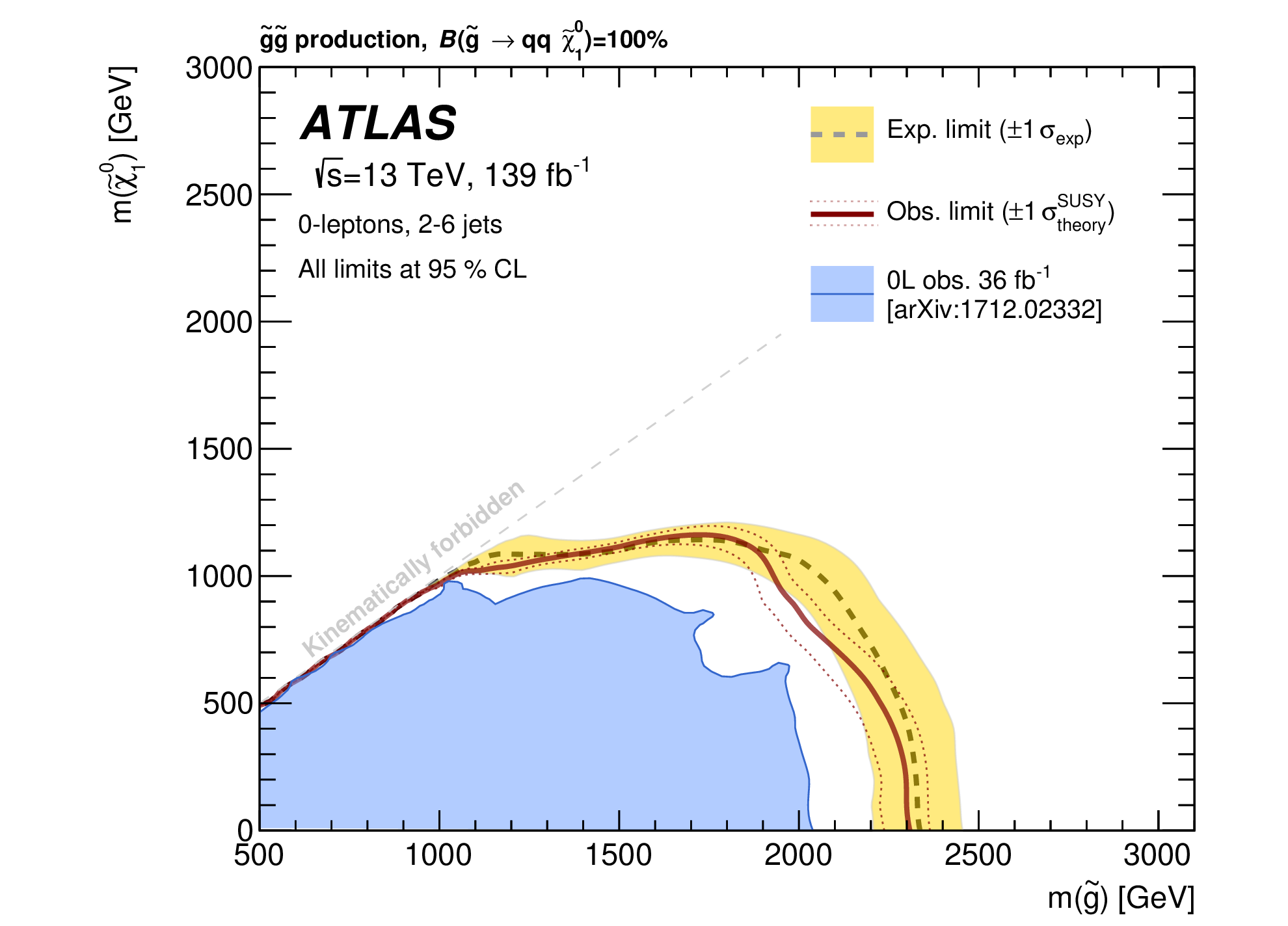
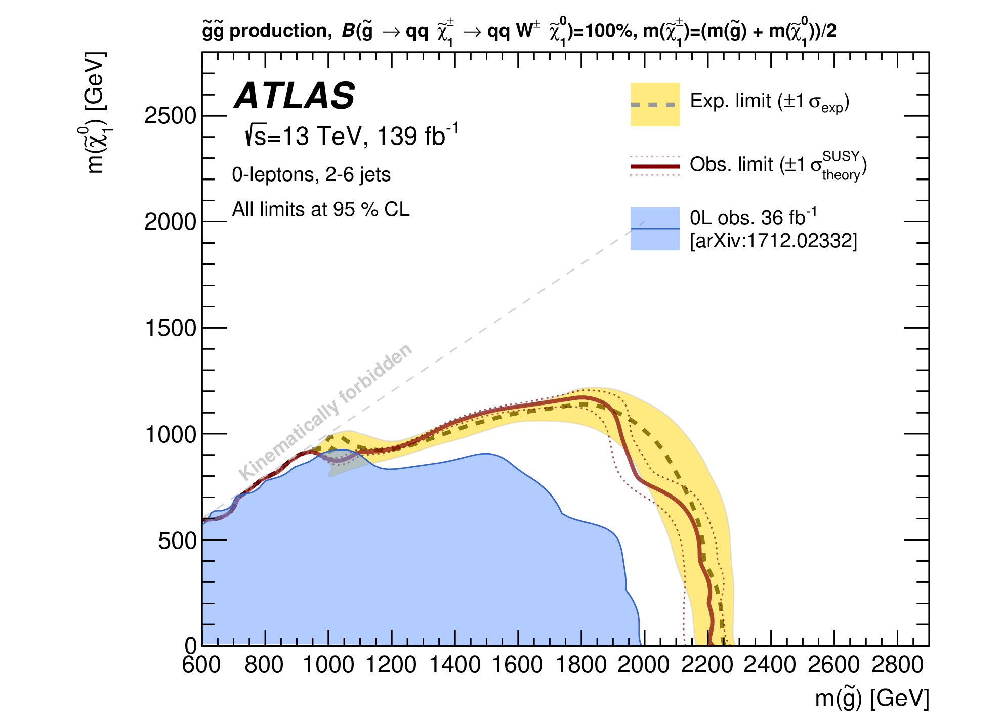
Searches for first two generation squarks and gluinos: The ATLAS collaboration has searched for squarks and gluinos in fully hadronic channel ($0l$ + jets + $\rm E{\!\!\!/}_{T}$ final states) based on full Run-II dataset ($\mathcal{L}=139\rm{fb}^{-1}$) using three strategies: multibin search, BDT search and model-independent search ATLAS:2020syg . Results were interpreted in various simplified scenarios where gluino can decay directly (${\widetilde{g}}\to q\bar{q}\widetilde{\chi}_{1}^{0}$) or via one step (${\widetilde{g}}\to q\bar{q}^{\prime}\widetilde{\chi}_{1}^{\pm}$) as shown in Fig. 1 of Ref. ATLAS:2020syg . Depending on the mass difference $(\Delta m({\widetilde{g}},\widetilde{\chi}_{1}^{0}))$, ATLAS has separated the events into four categories for these gluino decay modes. Eight independent BDT were trained to obtain the optimal sensitivity (see Table 7 of Ref. ATLAS:2020syg ). Among the three search strategies, the BDT search was the most robust tool, particularly effective in scenarios involving gluino decays via $q\bar{q}^{\prime}\widetilde{\chi}_{1}^{\pm}$, resulting in complex event topology with a large number of jets. The optimized BDT regions, chosen based on their BDT score, achieved the best sensitivity due to their ability to exploit the correlations between variables. In regions of the parameter space where the mass difference between the LSP - NLSP is small and approaches the kinematic limit, the multi-bin search is particularly effective and has excluded gluino and neutralino masses upto $\sim$ 900-1000 GeV (see Fig.5) from gluino pair production. For relatively light neutralino masses, the observed lower limit on the gluino mass reaches upto 2.3 (2.2) TeV for direct (one-step) gluino decay ATLAS:2020syg and is derived from the optimized BDT regions (see Fig.5). The same analysis has also excluded $m_{\widetilde{q}}$ upto 1.85 TeV for massless lightest neutralino considering the pair production of mass degenerate first and second generation squarks.

Figure 5: Exclusion limits in the $m_{\widetilde{g}}-m_{\widetilde{\chi}_{1}^{0}}$ plane, obtained using multi-bin search, BDT search and model-independent search, from gluino pair production for direct decays (${\widetilde{g}}\to q\bar{q}\widetilde{\chi}_{1}^{0}$) in the left panel and for one-step (${\widetilde{g}}\to q\bar{q}^{\prime}\widetilde{\chi}_{1}^{\pm}$) decay in the right panel ATLAS:2024fub .

Figure 6: Left: Distribution of BDT output form 13 TeV CMS data with $\mathcal{L}=59.8\rm{fb}^{-1}$ from stop pair production where $\Delta m({\widetilde{t_{1}}}-\widetilde{\chi}_{1}^{0})=50$ GeV and stop decays via $bf\bar{f}^{\prime}\widetilde{\chi}_{1}^{0}$ mode CMS:2023ktc .

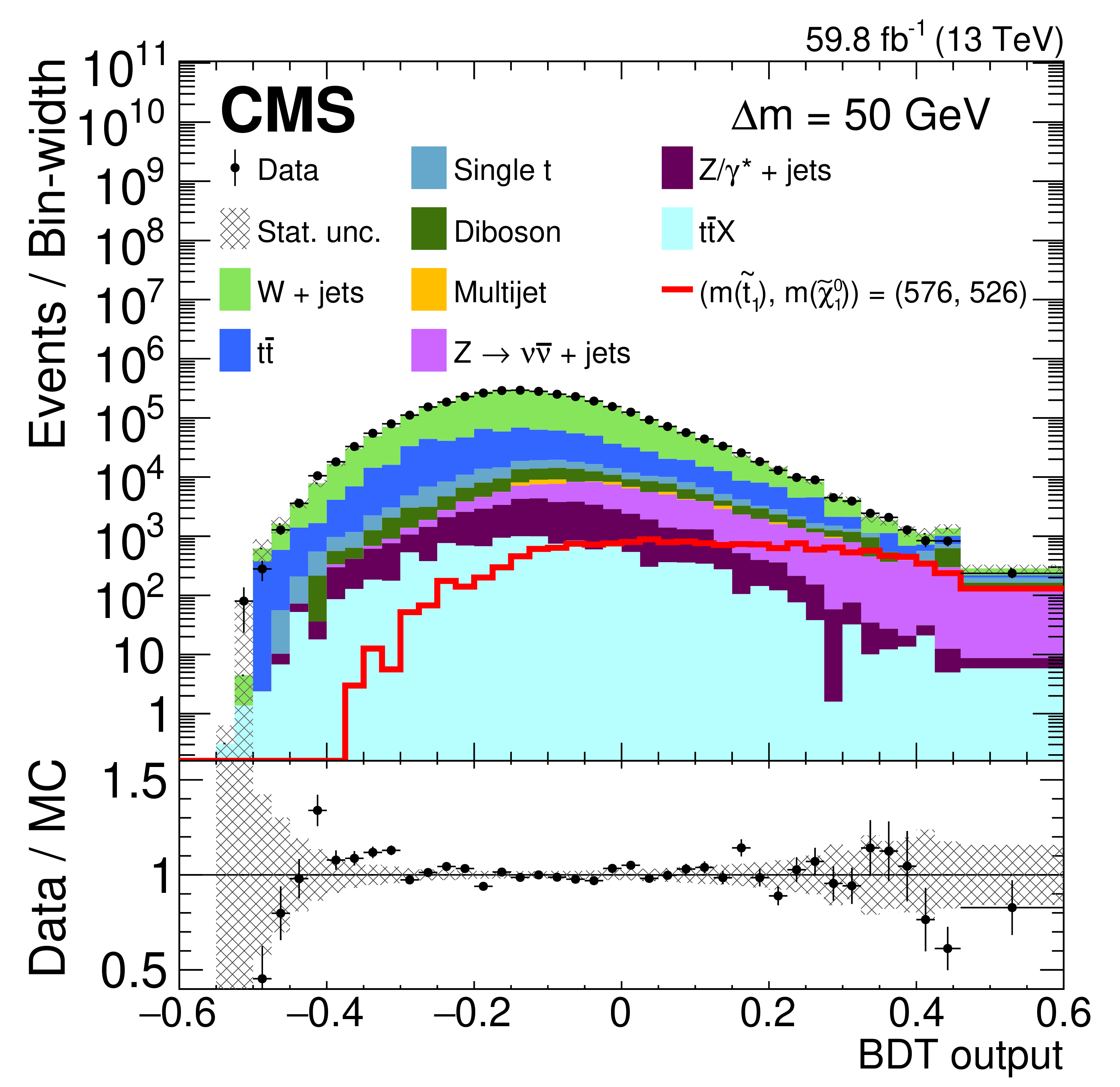
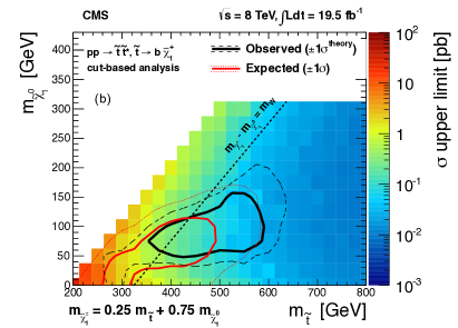
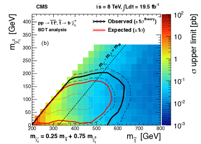
Searches for Stop: The light stop scenario is theoretically well-motivated Balazs:2004bu and also has a rich phenomenology. Both the ATLAS and CMS collaborations have looked for the lightest stop squarks (${\widetilde{t_{1}}}$) through all possible decay modes with various final states. The possible decay modes of stop are $t\widetilde{\chi}_{1}^{0}$, $b\widetilde{\chi}_{1}^{\pm}$, $bW\widetilde{\chi}_{1}^{0}$, $c\widetilde{\chi}_{1}^{0}$, $bf\bar{f}^{\prime}\widetilde{\chi}_{1}^{0}$. The last one (four body mode) may dominate in the compressed SUSY scenario where the other decay modes are kinematically forbidden and $c\widetilde{\chi}_{1}^{0}$ is suppressed. In a recent study, the CMS collaboration has used the BDT algorithms TMVA:2007ngy to optimize the separation between background and signal events CMS:2023ktc . The discriminating variables of signal and background processes have different correlations and CMS has performed the BDT analysis for different values of $\Delta m({\widetilde{t_{1}}}-\widetilde{\chi}_{1}^{0})$. The distribution of the score of multivariate analysis (the BDT discriminator value or BDT output) is shown in Fig.6 as obtained by CMS for $\Delta m({\widetilde{t_{1}}}-\widetilde{\chi}_{1}^{0})=50$ GeV. This BDT search has excluded $m_{\widetilde{t_{1}}}$ upto 480 and 700 GeV for $\Delta m$ = 10 and 80 GeV at 95$\%$ CL CMS:2023ktc . CMS had also implemented a BDT multivariate approach to define the signal regions for the analysis of stop pair production with subsequent ${\widetilde{t_{1}}}\to t\widetilde{\chi}_{1}^{0}$, and ${\widetilde{t_{1}}}\to b\widetilde{\chi}_{1}^{\pm}$ decays in Ref. CMS:2013phu . The comparison between the exclusion plots obtained by CMS CMS:2013phu for ${\widetilde{t_{1}}}\to b\widetilde{\chi}_{1}^{\pm}$ decay using cut-based and BDT methods are presented in the left and right panels of Fig.7.

Figure 7: The exclusion plot in $m_{\widetilde{t_{1}}}-m_{\widetilde{\chi}_{1}^{0}}$ plane for ${\widetilde{t_{1}}}\to b\widetilde{\chi}_{1}^{\pm}$ decay from cut-based (left panel) and BDT method (right panel) respectively CMS:2013phu .

A recent phenomenological work Jorge:2021vpo has expanded and improved the ATLAS analysis ATLAS:2020xzu for ${\widetilde{t_{1}}}{\widetilde{t_{1}}}$ pair production in the semileptonic channel where the stop squarks decay via 3 body mode $bW\widetilde{\chi}_{1}^{0}$. ATLAS has used a recurrent neural network (RNN) algorithm and excluded stop mass upto 710 GeV using 13 TeV LHC data with $\mathcal{L}=36.1\rm{fb}^{-1}$ ATLAS:2020xzu . The authors compared the performance of Logistic Regression, Random Forest, XGBoost and Neural Network algorithms in the Ref. Jorge:2021vpo at 13 TeV LHC with $\mathcal{L}=140\rm{fb}^{-1}$. It has been shown that in such compressed scenarios, XGBoost and Neural Network algorithms improve the signal significance more efficiently compared to other algorithms as well as the cut-and-count approach.

Figure 8: The post-fit BDT score distributions for the direct stau channel for BDT3 ATLAS:2024fub . The black arrow represents the BDT score selection for the SR-BDT3. Two SUSY benchmark points are shown with a dashed line. For more details, see Ref. ATLAS:2024fub .

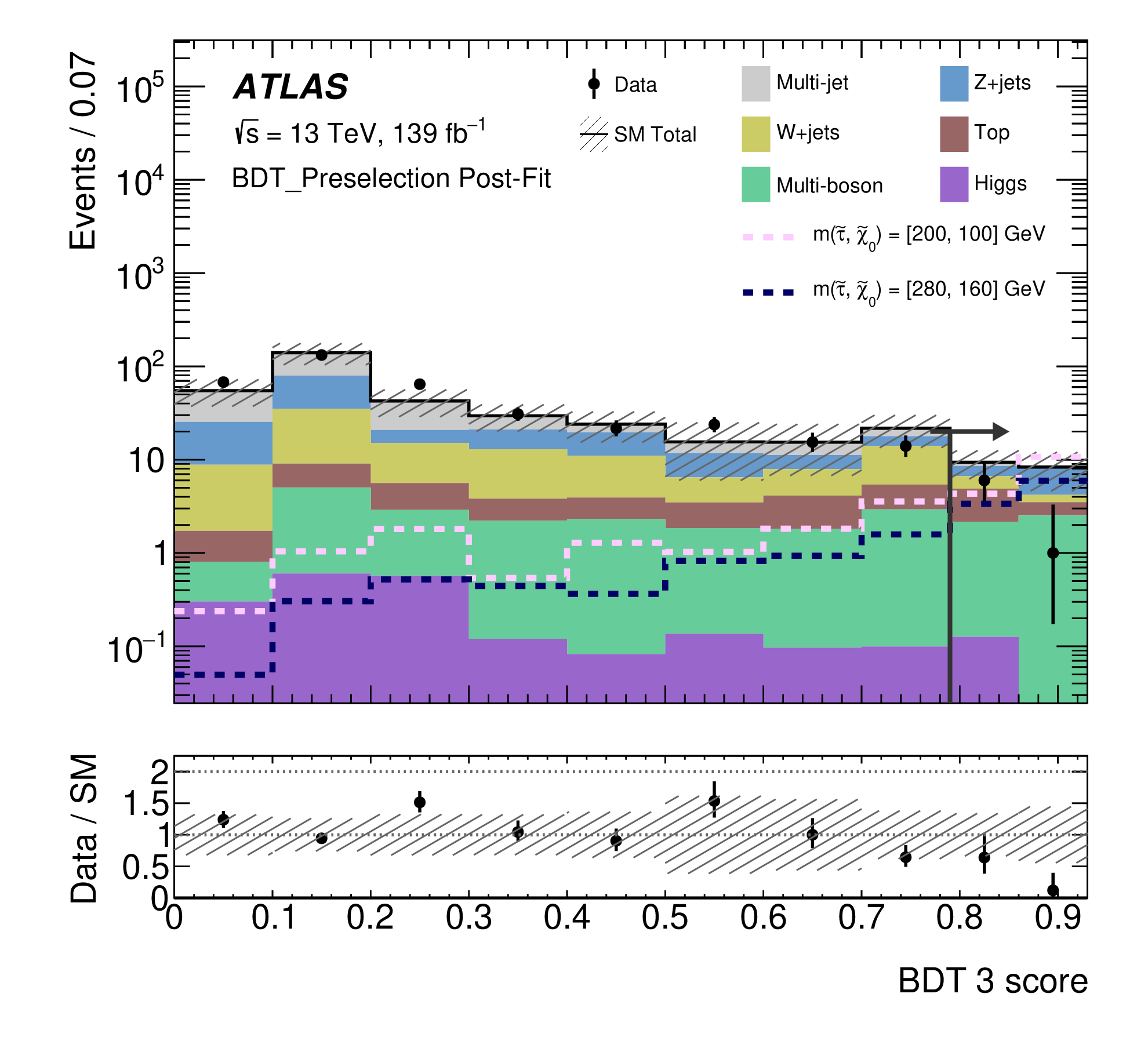
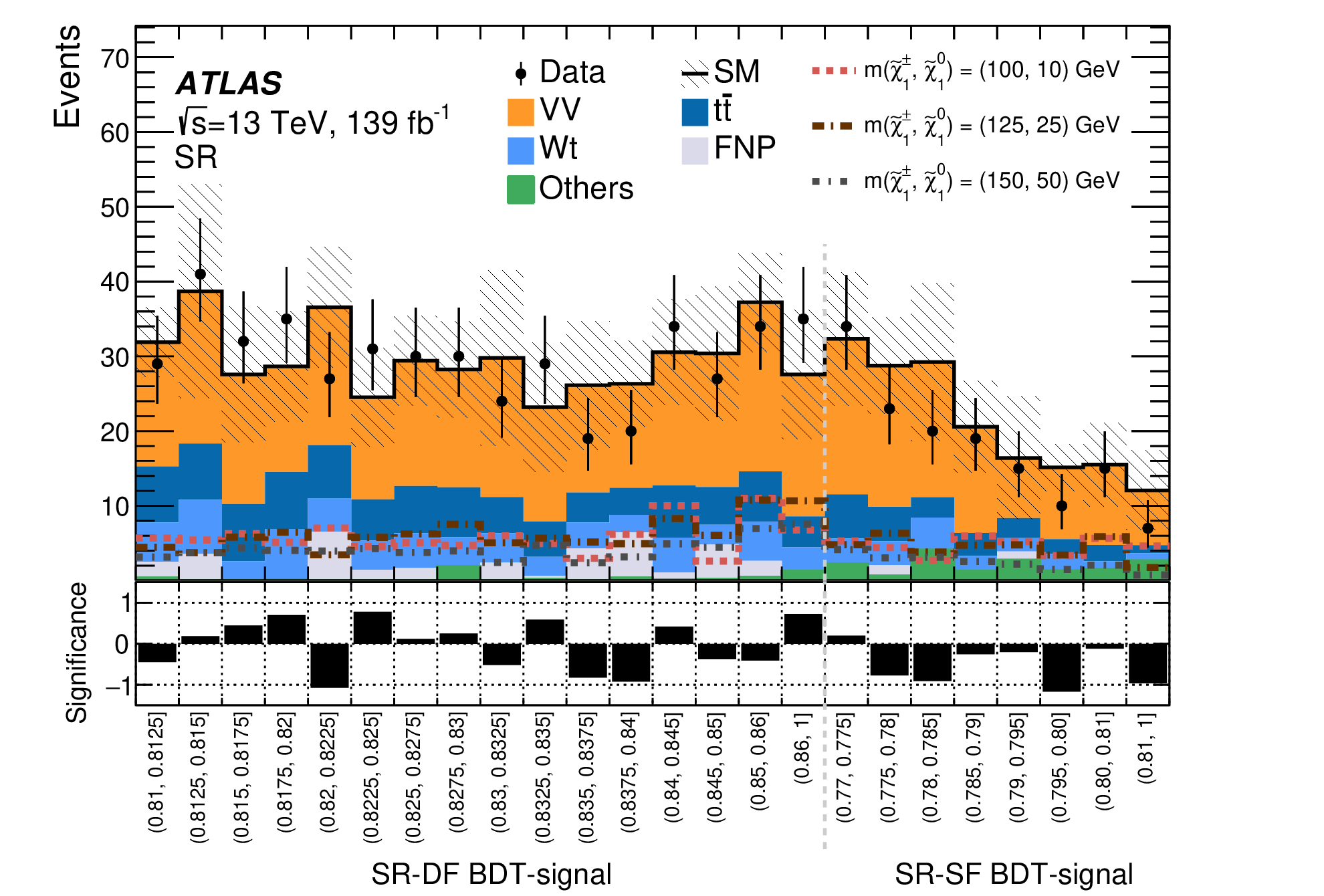
Searches of Electroweakinos and sleptons: Very recently, for the first time, the ATLAS Collaboration has reported the sensitivity of $\widetilde{\tau}_{R}$ only RPC SUSY scenarios with $2\tau+\rm E{\!\!\!/}_{T}$ final states using the LHC Run-II dataset with $\mathcal{L}=139\rm{fb}^{-1}$ ATLAS:2024fub . In this analysis, other scenarios with $\widetilde{\chi}_{1}^{\pm}\widetilde{\chi}_{1}^{\mp}$ and $\widetilde{\chi}_{1}^{\pm}\widetilde{\chi}_{2}^{0}$ pair productions also have been considered. The LightGBM package has been used to train multiple BDTs on the sensitivity of stau-LSP phase space. The ATLAS experiment has excluded $\widetilde{\tau}_{R}$ masses upto 350 GeV by improving the signal background separation through the use of BDT ATLAS:2024fub . The training was done for four BDT and for illustration purpose, we present the post-fit BDT score distribution for the signal region BDT3 ATLAS:2024fub in Fig.8 In another recent study, the ATLAS collaboration has looked for the chargino pair production via 2l + $\rm E{\!\!\!/}_{T}$ final states where the mass gap between the charginos and lightest neutralinos are close to W boson mass ATLAS:2022hbt . For this analysis, ATLAS has performed a multiclass GBDT classification using LightGBM NIPS2017_6449f44a , and signal regions are defined according to BDT scores (see Table 3 of Ref. ATLAS:2022hbt ). The observed and expected numbers of events are presented in Fig. 9 along with the significance. In the absence of any significant excess, ATLAS has excluded $m_{\widetilde{\chi}_{1}^{\pm}}$ up to 140 GeV at 95% CL for $\Delta m(\widetilde{\chi}_{1}^{\pm}-\widetilde{\chi}_{1}^{0})\sim 100$ GeV ATLAS:2022hbt .

Figure 9: The observed and expected number of events along with significance provided by ATLAS ATLAS:2022hbt is presented here.

In the Ref Cornell:2021gut , the authors have shown that gradient boosting algorithm can extend the 95% C.L. exclusion limits derived from traditional cut-based methods using an example of smuon pair production at the 13 TeV LHC. The authors have also studied the utility of various performance metrics (auc, ams, F-score etc.) using XGBoost toolkit, feature importance using SHAP package Shapley+1953+307+318 ; lundberg2018consistent in great details Cornell:2021gut . The possibility of constructing a general machine learning model that may be applied to probe a two-dimensional mass plane has also been examined in this work. In Alvestad:2021sje , the authors pointed out that XGBoost algorithm can significantly increase the detectability of a SUSY models with a gravitino type LSP and a metastable sneutrino NLSP by analyzing the events coming from the electroweakinos production along with the slepton productions. The possibility of probing the light Higgsinos, which are still allowed by LHC Run-II and LZ experiment data, at the upcoming HL-LHC run via XGBoost framework has been studied in Ref. Barman:2024xlc

Figure 10: Left: BDT score distribution obtained by ATLAS ATLAS:2018ntn for $m_{H^{\pm}}$ = 200 and 800 GeV along with SM backgrounds. Right: Expected (dotted line) and observed (hatched area) limits on tan$\beta$ as a function $m_{H^{\pm}}$ from the $H^{+}\to\tau\nu_{\tau}$ (red color) ATLAS:2018gfm and $H^{+}\to tb$ decay (black) ATLAS:2018ntn in the hMSSM scenario Djouadi:2013uqa

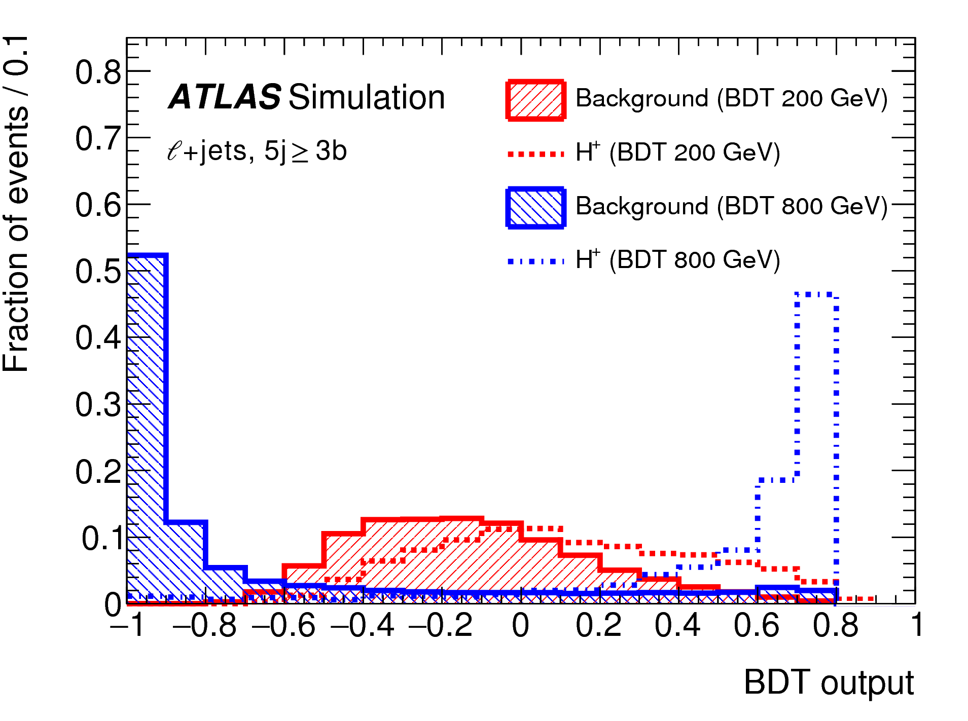
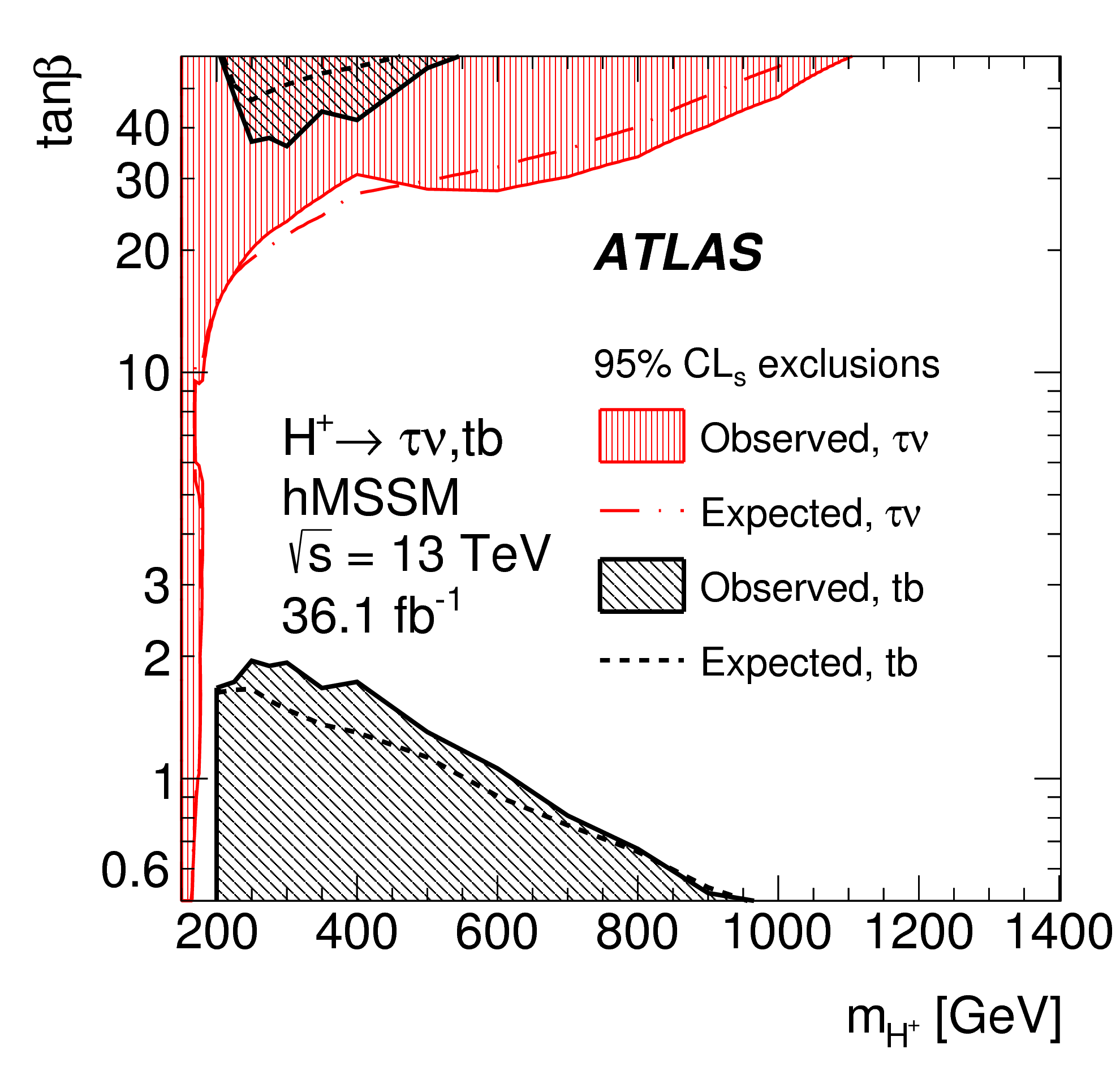
Searches of Heavy Higgs: The Minimal Supersymmetric Standard Model (MSSM) consists of two Higgs doublets and after electroweak symmetry breaking, the Higgs sector contains two CP even Higgs (h and H), one CP odd Higgs boson (A) and two charged Higgs bosons $H^{\pm}$. Extensive studies from LHC collaborations and phenomenological groups have already been performed for the Heavy Higgs searches. The implication of LHC results from 125 GeV Higgs boson searches and other heavy Higgs searches have been analyzed in Ref. Bagnaschi:2017tru ; GAMBIT:2017zdo ; Bhattacherjee:2015sga ; Barman:2016jov . The ATLAS collaboration has used the multivariate BDT analysis for the searches of charged Higgs ($H^{\pm}$) in Ref. ATLAS:2018ntn ; ATLAS:2018gfm . For $m_{H^{\pm}}>m_{top}$ and in the alignment limit, $H^{+}\to tb$ is the dominant decay mode and for large values of tan$\beta$, the branching ratio of $H^{+}\to\tau\nu_{\tau}$ becomes $\sim 10\%$. ATLAS and CMS both have looked for these final states where the dominant production mode is $pp\to tbH^{+}$ ATLAS:2018ntn ; ATLAS:2018gfm ; CMS:2020imj ; CMS:2019bfg . CMS collaboration has used a a multivariate BDT with gradient boost (BDTG) classifier within TMVA toolkit for $H^{+}\to tb$ mode CMS:2020imj . ATLAS has performed the training of the BDTs with the TMVA toolkit for different values of $m_{H^{\pm}}$ in various signal regions to discriminate the $H^{\pm}$ signal from the SM backgrounds with $1l(l=e,\mu)+n_{j}+m_{bjet}$ final states ATLAS:2018ntn . The BDT score distribution obtained from this analysis for signal benchmark points with $m_{H^{\pm}}$ = 200 and 800 GeV along with SM backgrounds are shown in Fig.10 (left panel) from the $1l+5j\geq$ 3b channel. For the $\tau\nu_{\tau}$ final states, training of the BDT has been performed using the FASTBDT algorithm Keck:2017gsv . The results ATLAS:2018gfm were interpreted in the $tan\beta$ - $m_{H^{\pm}}$ mass plane (see the right panel in Fig. 10). The limit comparison plot shows that at high tan$\beta$, stringent limits come from the $\tau\nu$ channel and at low tan$\beta$, tb channel is more effective for $m_{H^{\pm}}>200$ GeV.

The authors in Ref. Baer:2021qxa have studied the prospect of Heavy Higgs search in a radiatively-driven natural supersymmetric model where the neutral Heavy Higgs decays to $\widetilde{\chi}_{2}^{0}\widetilde{\chi}_{2}^{0}$ or $\widetilde{\chi}_{1}^{\pm}\widetilde{\chi}_{2}^{\mp}$ and give rise to $4l+\rm E{\!\!\!/}_{T}$ signature. Detecting this signature at the HL-LHC will be very difficult. But it is shown the conventional cut-based method can probe $m_{A},H$ upto 1.65 TeV at the future 100 TeV pp collider Baer:2021qxa with signal significance greater than 5$\sigma$. Using a multivariate analysis (BDT) within the TMVA toolkit, the authors also pointed out that the BDT algorithm improves the signal significance and heavy Higgs can be probed upto 2 TeV.

3.1.2 Searches for RPV SUSY scenarios using BDT

One of the key motivations for going beyond the RPC MSSM is its inability to provide an explanation for the neutrino oscillation phenomena. The RPV SUSY scenarios can explain the light neutrino masses and mixing Grossman:2003gq ; Davidson:2000uc ; Roy:1996bua ; Allanach:2007qc ; Diaz:2014jta ; Choudhury:2023lbp . The RPV SUSY models can also address the muon (g-2) anomaly Chakraborty:2015bsk ; Altmannshofer:2020axr ; Chakraborti:2022vds ; Hundi:2011si or flavor anomalies Trifinopoulos:2019lyo ; Domingo:2018qfg ; Das:2017kfo . Due to the presence of lepton and/or baryon number violating terms, the LSP becomes unstable and decays to SM particles. As a result, the final state contains less missing energy and a higher number of leptons and/or jets, depending upon the coupling. Although the ATLAS and CMS collaboration have mainly presented results in the RPC SUSY scenarios, there exist a few analyses, based on cut based method, involving strong or electroweak sparticles pair production with subsequent RPV decays ATLAS:2021yyr ; ATLAS:2021fbt ; ATLAS:2024kqk ; CMS:2017szl ; CMS:2021knz ; CMS:2018skt . A recent work Dreiner:2023bvs has summarized the possible gaps in RPV-MSSM searches at the LHC in great detail by meticulously classifying the various possible RPV-MSSM signatures at the LHC and analyzing both direct and indirect production of various LSPs, the authors have derived limits on sparticle masses.

Figure 11: Projected discovery ($5\sigma$) and exclusion ($2\sigma$) limits from the wino searches Choudhury:2023eje and slepton searches Choudhury:2023yfg at the HL-LHC are presented in the left and right figure respectively. In the left panel, the dark blue (violet) color refers to $2\sigma$ reach from the cut-based (ML) analysis and the light blue (violet) color represents $5\sigma$ reach from cut-based (ML) analysis Choudhury:2023eje . In the right panel, the light violet and blue color regions can be probed from the ML and cut-based analysis, respectively, at the $2\sigma$ level Choudhury:2023yfg .

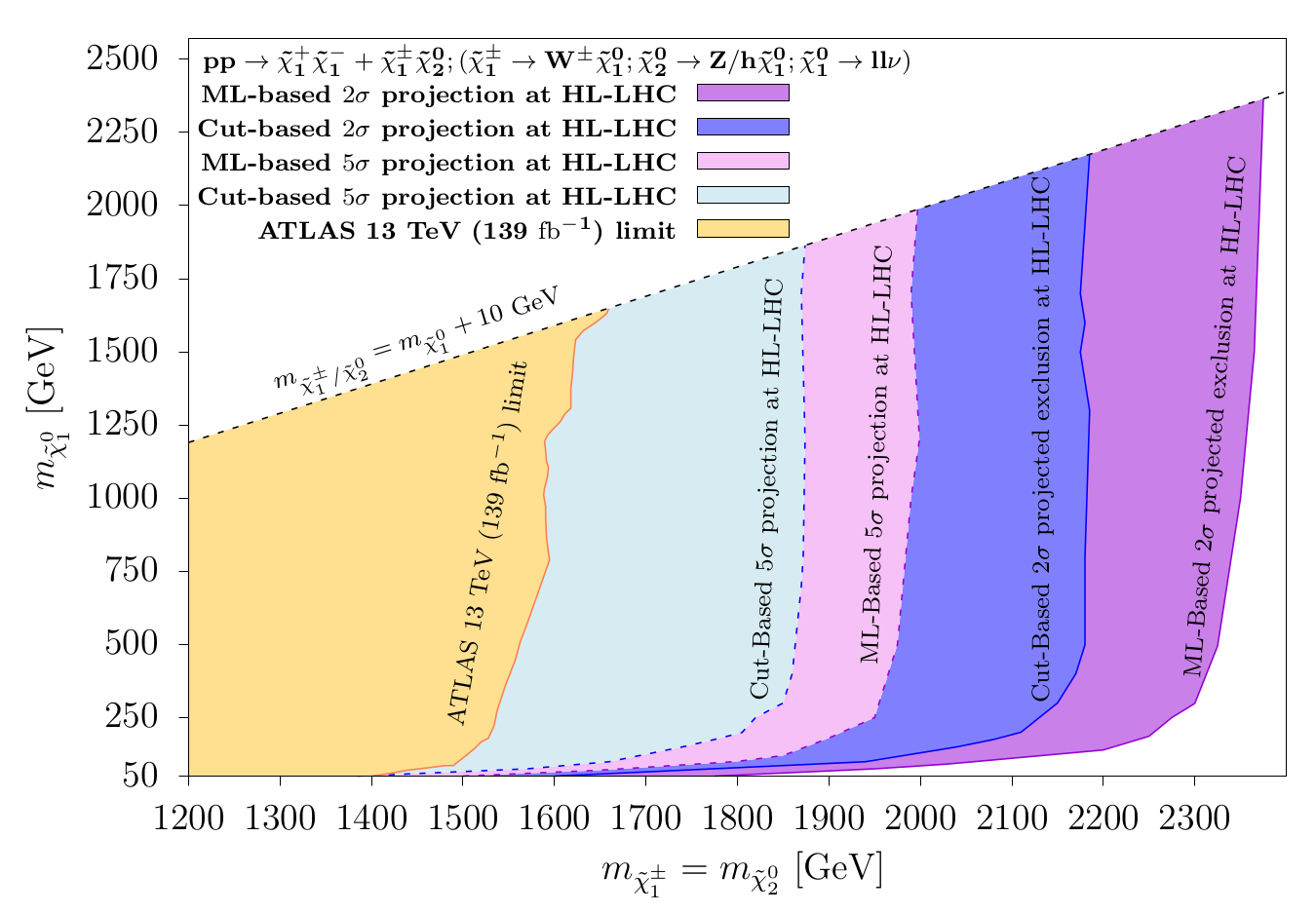
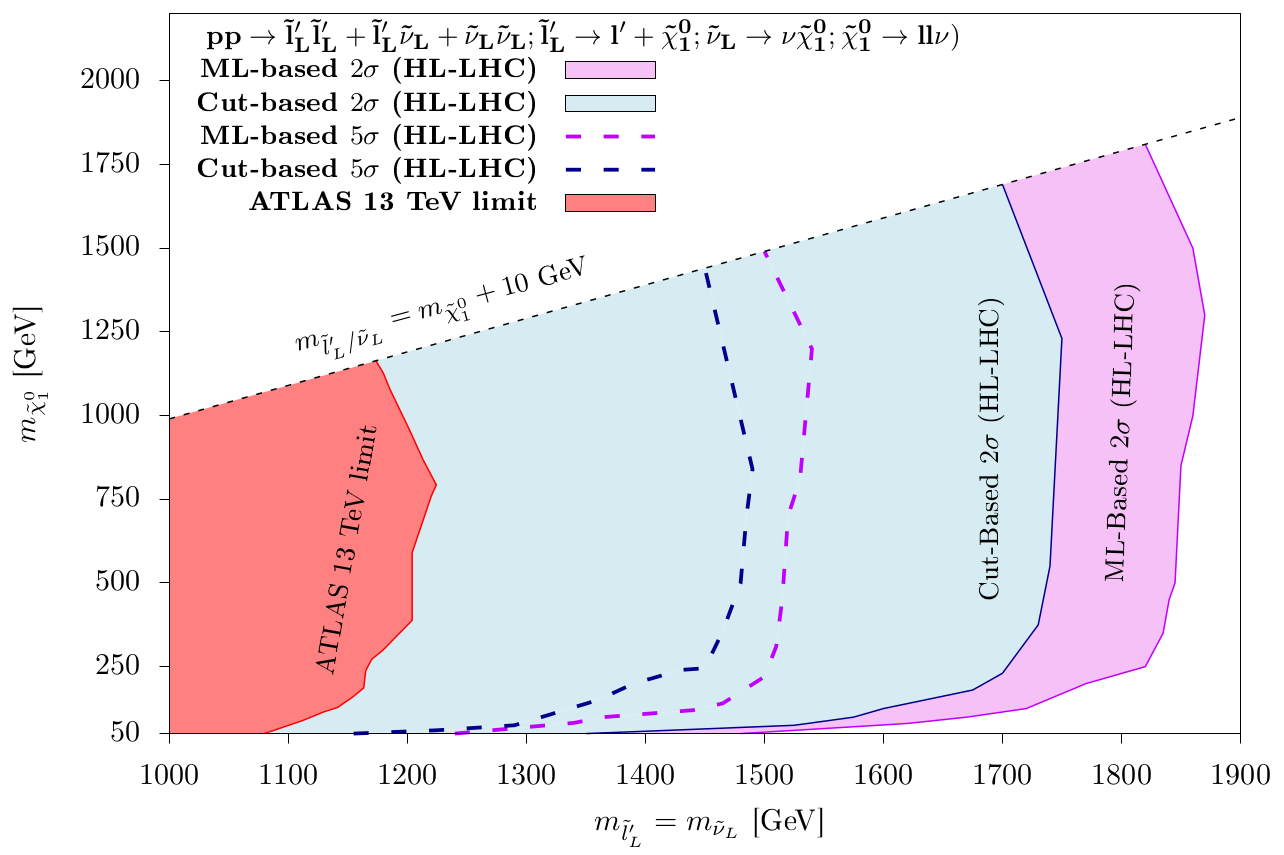
In the presence of non-zero trilinear couplings $\lambda_{ijk}$, the LSP decays into $l_{k}^{\prime\pm}l_{i/j}^{\prime\mp}\nu_{j/i}$, where $l^{\prime}=e,\mu,\tau$. Thus, the final states become leptonically enriched. For different choices of $\lambda_{ijk}$ couplings, the LHC collaborations have already derived limits on chargino and slepton masses (ATLAS:2021yyr, ). The yellow and red regions in the left and right panels of Fig.11 represent the excluded regions on chargino-LSP and slepton-LSP mass plane. The authors in Ref. Choudhury:2023eje ; Choudhury:2023yfg have extended the similar $4l+\rm E{\!\!\!/}_{T}$ final states in the context of the electroweak sparticle searches at the 14 TeV high-luminosity LHC (HL-LHC) and the proposed high-energy (27 TeV) upgrade of the LHC (HE-LHC). It has been shown that an optimized cut-based analysis will be able to exclude $m_{\widetilde{\chi}_{1}^{\pm}}$ upto 2.18 TeV at the HL-LHC from wino like $\widetilde{\chi}_{1}^{\pm}\widetilde{\chi}_{1}^{\mp}$ and $\widetilde{\chi}_{1}^{\pm}\widetilde{\chi}_{2}^{0}$ productions Choudhury:2023eje . The authors have further explored a multivariate analysis based on an Extreme Gradient BDT algorithm to improve the results further. The projected $2\sigma$ exclusion limit reaches up to 2.37 TeV and 4.0 TeV at the HL-LHC and HE-LHC, respectively, from the ML-based analysis Choudhury:2023eje (the dark violet color represents the $2\sigma$ reach for HL-LHC in Fig the left panel of Fig.11). In another recent work Choudhury:2023yfg , considering the pair and associated production of mass degenerate sleptons, the authors have studied the sensitivity of similar final state at the future LHC. The right panel of Fig.11 shows the discovery and exclusion reach on L-type slepton masses obtained for nonzero $\lambda_{121}$ and/or $\lambda_{122}$ coupling values Choudhury:2023yfg . It is observed that the projected exclusion limits on slepton and sneutrino masses at the HL-LHC (HE-LHC) are $\sim$ 1.85 (3.0) TeV from ML-based analysis. The ML algorithm shows significant improvement over cut-and-count method (see Fig.11). The work in Ref. Bhattacherjee:2023kxw has addressed the search prospect of long-lived particles in the RPV SUSY scenarios from the electroweakino pair production, where the LSP decays via UDD-type couplings. Utilizing the Gradient Boosting algorithm within XGBoost toolkit, the authors obtained that wino-like (higgsino like) $\widetilde{\chi}_{2}^{0}/\widetilde{\chi}_{1}^{\pm}$ with a mass of 1900 (1600) GeV and $\widetilde{\chi}_{1}^{0}$ with a mass greater than 800 (700) GeV can be probed for decay length ranging from 1 cm to 200 cm Bhattacherjee:2023kxw .

4 Decision Tree algorithms

The decision trees Breiman:1984jka are one of the simplest and most widely used classification and regression tools, which use inverted tree like structure with root on the top, to predict the value of an output by applying binary cuts in the feature space. Breiman et al. breiman ; Breiman:1984jka proposed “Classification and Regression Trees” (CART) algorithm for the implementation of decision trees (DT). The CART algorithm begins with the root-node consisting of the entire training dataset. It then proceeds to split the parent node into several branches or child nodes until the model can make a decision regarding the class of a given data point or it satisfies a predetermined stopping criteria. Through this binary splitting, the algorithm effectively partition the data into subsets. When the splitting criterion is met by the node, it is termed as a leaf.

Age	Chest pain	Blood pressure	weight	Diabetic	Risk of Heart
		(diastolic in mmHg)	(Kg)		disease
27	No	80	75	No	low
65	No	70	71	No	low
45	Yes	90	85	Yes	high
80	Yes	78	55	Yes	high
54	No	100	94	Yes	high
40	No	80	68	Yes	low

Table 2: A dataset with 6 entries whether a person suffers from heart disease or not. The right most column represents the final output whether a person suffers from heart disease based on the input features.

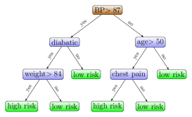
We demonstrate this process with a medical science example in the Table. 2 regarding the risk of heart disease of a person. In medical science, the risk of being diagnosed with a heart disease primarily depends on the person’s age, blood pressure, weight, whether the person is diabetic or not etc. The initial five columns denote input features, while the last column signifies the resulting outcome. A decision tree, depicted in Fig. 12, is constructed using this dataset. In the tree visualization, the root node is depicted in brown, leaf nodes in green, and general nodes in blue.

Figure 12: A decision tree based on the dataset given in Table. 2 is shown here. The root node is marked with brown color. Ordinary nodes and leaf nodes are denoted using blue and green colors, respectively.

In the context of HEP, the goal for DT algorithm is mainly to classify an entry as a signal or background. For classification problem, the journey from the root-node to the leaf-node signifies a series of cuts which determines whether an entry is classified as signal or background depending upon the characteristics of the leaf-node. Each leaf can be assigned a purity value, calculated as $p=S/(S+B)$ where $S$ and $B$ represent the sum of weights of the signal and background events contained within that leaf. Depending upon this value of purity the events in that leaf can be identified as signal or background ( if $p>0.5$, it is identified as signal; otherwise, it is classified as background.) At each node, the feature and its corresponding threshold value determine the subsequent splitting of the node. The selection of the feature and its threshold value depends on the decrease in impurity. The commonly used impurity functions include the misclassification error , the cross entropy breiman ; Breiman:1984jka and the Gini index of diversity gini ; ceriani2012origins , all of which are determined by the purity of signal and background. Among these impurity function, the most popular one is the Gini index which performs similar to entropy. In HEP, generally we try to optimize the signal significance $S/\sqrt{S+B}$ or $S/\sqrt{B}$ by applying Cross section significance or excess significance which is defined as $-S^{2}/(S+B)$ and $-S^{2}/B$ respectively. On the other hand, regression tress trees split nodes based on minimizing the Sum of Squared Errors (SSE). The tree-growing process is stopped using stopping criteria. The stopping condition may include several criteria, such as reaching a maximum tree depth, maximum number of leaf nodes, ensuring a minimum number of instances within each leaf node, insufficient improvement through further splitting, or achieving complete splitting, where all events within the node belong to the same class. Sometimes, even before reaching the maximum allowed depth or number of nodes, early stopping criteria are used to prevent overfitting and improve the generalization.

After constructing the tree, predictions are generated by navigating from the root node to a leaf node that matches the input data. Although decision trees are adept at modeling training data, they are known for their susceptibility to instability. Overfitting to the training sample can make a decision tree overly sensitive to minor variations in inputs, reducing its effectiveness for unfamiliar events or data, as it heavily relies on the training set. Pruning refers to the process of cutting irrelevant branches or reducing the size of DT by removing nodes and branches that do not significantly improve the predictive performance of unseen data. Pruning a tree is crucial for reducing instability, avoiding overfitting, and enhancing the model’s ability to generalize with new data. “Pre-pruning” is similar to the early stopping we have already discussed above. “Post-pruning” involves constructing an extensive tree initially and subsequently eliminating irrelevant branches. These branches are pruned by converting an internal node and all its offspring into leaves, thereby eliminating the corresponding subtree. There are several pruning algorithms like expected error pruning, reduced error pruning QUINLAN1987221 and cost-complexity pruning which is a part of the CART algorithm Breiman:1984jka .

There is another method to handle the instability of the decision trees, which is called “ensemble learning”. Ensemble learning addresses this by combining predictions from multiple trees, potentially boosting discriminatory power. Techniques such as bagging, boosting, and random forests fall under this framework, offering various ways to improve model performance. The combination of aggregation and bootstrapping is known as “bagging” or bootstrap aggregating. Initially, a new dataset is created by randomly sampling data from the original dataset, ensuring that the new dataset contains the same number of samples as the original dataset. One important point is that individual samples from the original dataset can appear multiple times in the new dataset. This process is known as ”bootstrapping.” Subsequently, multiple trees are constructed based on the features of the new dataset. This procedure is repeated several times until the algorithm generates and aggregates a considerable number of trees. In the upcoming subsection, we will summarize the following DT algorithms that utilize “ensemble learning” techniques. Specifically, we will focus on Random Forest, which is an extension of bagging and boosting algorithms. Within the boosting category, our attention will be on AdaBoost, as well as two Gradient boosted decision tree (GBDT) algorithms: XGBoost and LightGBM.

4.1 Random Forest

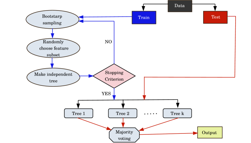
The Random forest algorithm Breiman:2001hzm is a robust ensemble learning method used for regression and classification jobs. The key concept of the Random forest algorithm is to create an ensemble (forest) of decision trees and to select the prediction voted by the majority/averaging of all those trees depending upon the classification/regression task. For a better overall outcome, a subset of input data is passed through each decision tree. Randomizing the training variables helps to obtain better accuracy. Initially, a new dataset is generated for a given input dataset with $N$ samples. The algorithm randomly selects a sample and adds it as the first entry of the new dataset. This process iterates for $N$ times. It may be noted that one particular sample can occur more than once in the new dataset. This process is called “bootstrapping”. For a given input feature set $x_{i}$ where $i=1,\dots,m$, decision trees are made taking a random subset of features $n$, such that $n<m$. Based on these features, a tree is made. This process repeats several times till the algorithm generates and aggregates a large number of trees. The aggregation, together with bootstrapping, is referred to as “bagging”. Among all the trees, the outcome with the majority of votes is selected as the model prediction for classification problems. For regression tasks, the final outcome is calculated by averaging the predictions of all the decision trees. The model outcome depends on the hyperparameters, such as the number of trees the algorithm grows, the maximum depth of a tree, the maximum number of leaf nodes a tree can have, etc. The creation of a new tree is an iterative process, and it does not stop until the algorithm meets its stopping criterion (a pre-determined number of trees the algorithm can grow, which is fixed by the user). A flow chart for the Random Forest algorithm is shown in Fig. 13.

Figure 13: Flow-chart for Random Forest algorithm for classification tasks. For regression tasks, the final outcome is calculated by averaging instead of majority voting.

To illustrate this point, let us consider a sample dataset (Table. 3) for a supersymmetric (SUSY) signal with the Standard Model background, where the signal and background are labeled as 1 and 0, respectively. We have considered the transverse momentum of leading and sub-leading lepton ($p_{T}^{l_{1}}$ and $p_{T}^{l_{2}}$) and the leading jet ($p_{T}^{j_{1}}$), missing transverse energy ($\rm E{\!\!\!/}_{T}$) and $\Delta R$ (where $\Delta R=\sqrt{(\Delta\eta)^{2}+(\Delta\phi)^{2}}$, $\eta$ and $\phi$ are the pseudorapidity and azimuthal angle, respectively.) between leading and sub-leading lepton ($\Delta R(l_{1},l_{2})$) as input features.

$p_{T}^{l_{1}}$	$p_{T}^{l_{2}}$	$p_{T}^{j_{1}}$	$\rm E{\!\!\!/}_{T}$	$\Delta R(l_{1},l_{2})$	Label
55.1	45.3	75.2	180.4	1.5	1
25.7	20.3	14.5	138.3	1.4	0
65.2	52.7	88.3	201.7	1.2	1
45.9	39.6	55.7	147.2	1.4	1
46.2	42.9	35.9	151.1	1.7	0
40.8	31.5	41.9	130.6	1.4	0
40	33	65	155	1.6	0

Table 3: Dataset to classify signal and backgrounds for various input features. The output (rightmost column) is 1 for the signal and 0 for the background. The first six labeled entries are training data and the test data is colored in light blue. Here, $p_{T}^{l_{1}}$, $p_{T}^{l_{2}}$, $p_{T}^{j_{1}}$ and $\rm E{\!\!\!/}_{T}$ are in units of GeV.

The label (class) corresponding to each entry is written in the gray-shaded column at the right. The first six entries are training data, and the light-blue colored data is test data. A forest of decision trees is made (Fig. 14) from the training data of Table. 3.

Figure 14: A sample forest of three trees made from the training dataset given in Table. 3. The prediction for the test data (Table. 3) and its direction of flow is shown in blue color.

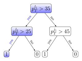
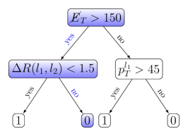
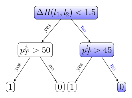
Test data generates predictions as it passes through each tree in the forest. For our example, the outcome of each tree is marked with a blue color when the test data from Table. 3 passes through them. In our example, two of the three trees classify that entry as a background ($0$), and one classifies it as a signal ($1$). Since the majority is “0”, the prediction for this particular entry is “$0$” or background. It is worth noting that the predicted output matches the actual data, which signifies the accuracy of the algorithm.

Random forest can deal with both classification and regression problems and it can handle high dimensional data very well. The accumulation of numerous decision trees and random feature selection provides better accuracy and reduces overfitting. On the other hand, the random forest algorithm is computationally expensive and time-consuming.

4.2 AdaBoost

Decision trees are the base learner for Random Forest and many other algorithms. The learners can be weak or strong depending on their prediction accuracy. Poor prediction accuracy is associated with weak learners, whereas a strong learner yields better model prediction accuracy. While it is hard to predict an output only through a weak learner, a combination of such weak learners can be made into a strong learner. At each step, the misclassified instances are provided with a larger weightage, resulting in better accuracy at the final step. This process is called “Boosting”. AdaBoost freund1999short ; wang2012adaboost works on the basic principle of the boosted decision tree (BDT) algorithm. The term AdaBoost originates from Adaptive Boosting, as the misclassified events are given a larger weightage, while the correctly classified events are given a smaller weightage in this algorithm. Freund and Schapire introduced the AdaBoost algorithm Freund:1997xna in 1995 and from then, it has been widely used in many scenarios including the HEP analysis.

Figure 15: Flow chart of AdaBoost algorithm.

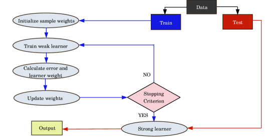
A set of labeled training data $\{x_{i},\hat{y}_{I}\}$ where $x_{i}$ denotes the input features and $\hat{y}_{i}$ stands for the label, is fed into the algorithm. Here $i=1,2,3...m$, and each $x_{i}$ and $\hat{y}_{i}$ belong to domains $X$ and $Y$, respectively ($x_{i}\in X,~{}\hat{y}_{i}\in Y=\{-1,+1\}$). For simplicity, here we have chosen binary classification to elaborate on, and the classes are denoted as $+1$ and $-1$. The base learner is repeatedly called by the algorithm for $t=1,\dots,T$ iteration. It may be noted that $T$ denotes the hyperparameter number of trees/estimators. The weight of the $i^{\text{th}}$ sample in $t^{\text{th}}$ iteration is denoted by $w_{t}(i)$. In the beginning, all samples are assigned the same weight. At each iteration, the learner is compelled to focus on the incorrectly classified event by giving larger weightage to the incorrectly classified events. The learner constructs a weak hypothesis $h_{t}:X\rightarrow\{-1,+1\}$ for $w_{t}$ with the lowest error, where the error is given by $\epsilon_{t}=\sum_{i\colon h_{t}(x_{i})\neq\hat{y}_{i}}w_{t}(i)$. The algorithm next assigns a parameter $\alpha_{t}=\eta\ln(\frac{1-\epsilon_{t}}{\epsilon_{t}})$ to the weak hypothesis, $h_{t}$, which is a measure of performance of $h_{t}$. Here, $\eta$ acts as the learning rate or shrinkage coefficient, which is a measure of the strength of boosting. It is worth noting that for $\epsilon_{t}\leq 1/2$, $\alpha_{t}\geq 0$, and $\alpha_{t}$ increases with decreasing $\epsilon_{t}$. The weight, $w_{t}$, is then modified. A larger weight (multiplying $w_{t}$ by $e^{\alpha_{t}}$) is given for the misclassified events ($h_{t}(x_{i})\neq\hat{y}_{i}$) and a smaller weight (multiplying $w_{t}$ by $e^{-\alpha_{t}}$) is given to the correctly classified events ($h_{t}(x_{i})=\hat{y}_{i}$). After completion of $T^{\text{th}}$ iteration (stopping criterion), the weighted majority of all $T$ weak hypotheses is chosen to be the final hypothesis or strong learner, $H(x)$. The flow chart of the AdaBoost algorithm is presented in Fig. 15.

The ability of AdaBoost to create a strong learner by combining several weak learners by weighted data sampling makes it more efficient than the Random forest algorithm. Furthermore, the AdaBoost training process leads to faster convergence in many scenarios. However, while dealing with complex datasets or when the base learner is too complex, AdaBoost is susceptible to overfitting.

4.3 XGBoost

A general gradient boosting decision tree (GBDT) algorithm uses gradient descent to minimize the loss function. In addition to the boosting, it optimizes the algorithm to find the local minima of a differentiable loss function. A loss function signifies the quantitative goodness of the model prediction. The “eXtreme Gradient Boost” or XGBoost Chen:2016btl is an extension of the GBDT algorithm. Here, the algorithm utilizes the second-order derivatives of the convex loss function, in contrast to a general GBDT algorithm where only the first-order derivative is used. The flow of the XGBoost algorithm can be divided into two parts: the first consists of boosting by obtaining optimal leaf score or weight for tree growth, and the second is optimizing the algorithm for smoother operation. In the following, we discuss them.

XGBoost uses a regularized objective; in simpler terms, one regularization or penalty term is added with the objective function, and it helps to prevent overfitting. For a given dataset $\mathcal{D}=\{x_{i},\hat{y}_{i}\}$ with $m$ features and $n$ entries such that $x_{i}\in\mathbb{R}^{m}$, the predicted output for $K$ number of trees is Chen:2016btl

$$y_{i}=\phi(x_{i})=\sum_{k=1}^{K}f_{k}(x_{i}),\hskip 28.45274ptf_{k}\in\mathcal{F},$$ (11)

where $\mathcal{F}=\{f(x)=w_{q(x)}\}$ is the tree function space. The mapping for a feature $x$ to the corresponding leaf index is denoted by the function $q(x)$ and $w\in\mathbb{R}^{T}$ where $T$ is the number of leaves at $k^{\text{th}}$ tree. Here, $w_{k}$ is the score of $k^{\text{th}}$ leaf. A regularization term ($\Omega$) is added to the loss function ($l$) and the new objective function becomes Chen:2016btl

$$\mathcal{L}(\phi)=\sum_{i=1}^{n}l(y_{i},\hat{y}_{i})+\sum_{k=1}^{K}\Omega(f_{k})$$ (12)

where $\Omega(f)=\gamma T+\frac{1}{2}\lambda\Arrowvert w\Arrowvert^{2}$. Here, $\gamma$ is the minimum loss reduction term used to further divide a leaf node, and $\lambda$ is a ridge regularization term acting on the leaf weights. A higher value of $\lambda$ and $\gamma$ results in a more conservative algorithm. As the number of leaves increases within a tree, the objective function is subsequently increased. Consequently, this makes minimizing the objective more challenging. To overcome this issue, we add $f_{t}$ to minimize the objective.

$$\mathcal{L}^{(t)}=\sum_{i=1}^{m}l(\hat{y}_{i},y_{i}^{(t-1)}+f_{t}(x_{i}))+\Omega(f_{t})$$ (13)

where $\mathcal{L}^{(t)}$ and $y_{i}^{t}$ denote the objective and prediction for $i^{\text{th}}$ entry at $t^{\text{th}}$ iteration. The next step is to optimize the objective function, and for that, $\mathcal{L}^{(t)}$ is expanded in the Taylor series up to the second order Chen:2016btl

$$\mathcal{L}^{(t)}\simeq\sum_{i=1}^{n}[l(\hat{y}_{i},y_{i}^{(t-1)})+g_{i}f_{t}(x_{i})+\frac{1}{2}h_{i}f_{t}^{2}(x_{i})]+\Omega(f_{t})$$ (14)

where $g_{i}=\partial_{y_{i}^{(t-1)}}l(\hat{y}_{i},y_{i}^{(t-1)})$ is called the gradient and $h_{i}=\partial^{2}_{y_{i}^{(t-1)}}l(\hat{y}_{i},y_{i}^{(t-1)})$ is called the hessian. Let $I_{j}=\{i|q(x_{i})=j\}$ be the set of instances where $i^{\text{th}}$ instance is mapped to $j^{\text{th}}$ leaf with tree structure $q(x_{i})$. Eq.(14) can be written as Chen:2016btl

$$\tilde{\mathcal{L}}^{(t)}(q)=\sum_{j=1}^{T}[(\sum_{i\in I_{j}}g_{i})w_{j}+\frac{1}{2}(\sum_{i\in I_{j}}h_{i}+\lambda)w_{j}^{2}]+\gamma T$$ (15)

The optimal weight of the $j^{\text{th}}$ leaf, $w_{j}^{\ast}$ can be written as

$$w_{j}^{\ast}=\frac{-\sum_{i\in I_{j}}g_{i}}{\sum_{i\in I_{j}}h_{i}+\lambda}$$ (16)

and the minimum value of $\tilde{\mathcal{L}}^{(t)}(q)$ is

$$\tilde{\mathcal{L}}^{(t)}(q)=-\frac{1}{2}\sum_{j=1}^{T}\frac{(\sum_{i\in I_{j}}g_{i})^{2}}{\sum_{i\in I_{j}}h_{i}+\lambda}+\gamma T$$ (17)

Figure 16: Flow-chart for XGBoost algorithm

and it represents a quantitative measure of the goodness of the tree structure $q$, which is analogous to the impurity score. A smaller value of $\tilde{\mathcal{L}}^{(t)}(q)$ means a better tree structure. While it is non-trivial to count all possible trees to find the tree with the maximum impurity score, the use of a greedy algorithm eases the scenario. From a single leaf with $I$ instances, left and right branches are made with instances $I_{L}$ and $I_{R}$, respectively, such that $I=I_{L}\cup I_{R}$. It chooses the split with the highest reduction in loss. After the splitting, the loss reduction can be quantified as Chen:2016btl

$$\mathcal{L}_{split}=\frac{1}{2}\bigg{[}\frac{(\sum_{i\in I_{L}}g_{i})^{2}}{\sum_{i\in I_{L}}h_{i}+\lambda}+\frac{(\sum_{i\in I_{R}}g_{i})^{2}}{\sum_{i\in I_{R}}h_{i}+\lambda}-\frac{(\sum_{i\in I}g_{i})^{2}}{\sum_{i\in I}h_{i}+\lambda}\bigg{]}-\gamma$$ (18)

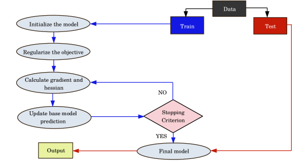
As we can see, XGBoost uses the second order derivative ($h_{i}$) along with gradient ($g_{i}$) of the loss function for boosting, which is different from other GBDT algorithms. We present the flow chart of the XGBoost algorithm in Fig.16. Finding the optimal split for a node is a non-trivial task, especially for large and complex datasets. XGBoost uses several split-finding algorithms. For a relatively simple dataset, it uses a “basic exact greedy algorithm” Chen:2016btl where it goes over all possible splits and finds the best one. However, for a large dataset, this technique results in a trade-off with reduced efficiency. To handle this, the algorithm divides the dataset into several percentile or weighted quantile buckets, treats each bucket separately through parallel learning and finds the best split. To deal with sparse data, XGBoost invokes the “sparsity-aware split algorithm,” where it enumerates the gain by going in both directions in a split and chooses the one with maximum gain. These features of XGBoost to tackle such complexities in a dataset make it scalable to almost all scenarios and popular among data scientists.

4.4 LightGBM

Simple gradient-boosting techniques have been quite successful so far. A common attribute of GBDT is to enumerate over all instances in dataset for each feature to find the optimal split. As data complexity and size increase, GBDT faces challenges in efficiency and accuracy. To overcome this issue, novel techniques are implemented upon simple GBDT algorithm, namely, (i) leaf-wise tree growth, (ii) Gradient-based one-sided sampling (GOSS), (iii) histogram splitting, and (iv) Exclusive feature bundling (EFB). The new algorithm that incorporates these new techniques with GBDT, developed by Microsoft, is referred to as Light Gradient Boosting Machine-learning or LightGBM ke2017lightgbm . In the following, we discuss the key concepts of LightGBM:

Leaf-wise tree growth: The attribute that fundamentally separates LightGBM from common GBDT is that it is based on “leaf-wise tree growth” (demonstrated in the right panel of Fig.17). The leaf node that provides maximum loss is split by the algorithm, and this process is repeated. In this case, one leaf may branch deeper than the other while both of them are coming from the same root node. The general GBDT algorithm is based on “depth-wise tree growth” or “level-wise tree growth”(as shown in the left panel of Fig.17), where trees are split horizontally at each level, and it expands every node at the same level before going to the next round.

Figure 17: Schematics for depth-wise and leaf-wise tree growth. The root node is colored brown, while the leaf nodes are marked green. Ordinary nodes are colored in blue.

Gradient-based one-sided sampling (GOSS): In GBDT, the smaller the gradient is, the better the fit becomes. In this technique, a subset of dataset is created by mostly retaining the instances with higher gradients and discarding (by random sampling) instances with smaller gradients. GOSS retains a percentage ($a\times 100\%$) of data with the highest gradient and randomly selects $b\times 100\%$ data from the rest and creates a new subsample, given $a,b\in[0,1]$. While calculating the information gain, the algorithm multiplies a factor $\frac{1-a}{b}$ to the instances with a smaller gradient. The under-trained instances thus get more attention even though no initial weight is associated with the original dataset.

Histogram splitting: For a tree branching, LightGBM algorithm bins the feature values into two or more sets rather than evaluating all potential split points for every feature. Let us suppose for a given dataset, there exists an input feature, “Age,” where the entries are 40, 45, 47, 50, 65, 72, 75, 80. The common approach for GBDT while creating a decision tree is to sort the value for which the optimal prediction is achieved. In the case of histogram splitting, the algorithm splits the dataset into two or more bins or buckets, say, age group 40-60 and 61-80 and then proceeds with the analysis. It makes the algorithm faster.

Exclusive feature bundling (EFB): The complexity of an algorithm increases with increasing input features. To improve efficiency, the algorithm looks for exclusive features in a given dataset (features that do not take non-zero values at the same time). To illustrate this point, let us suppose a binary dataset has a feature column for the gender of the person in a given entry. If we set the male to $1$ then the female is automatically set to $0$ and vice-versa. Both cannot take the same value simultaneously. EFB carefully combines these exclusive features and creates a new bundle, thus effectively reducing the input features without sacrificing accuracy.

Figure 18: Flow-chart for LightGBM algorithm

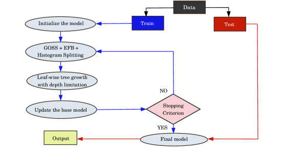
The flow-chart of LightGBM algorithm is shown in Fig. 18. LightGBM algorithm turns out to be more efficient in terms of time consumption compared with XGBoost while maintaining a competitive accuracy. Due to its histogram-based approach, LightGBM uses less memory, making it more efficient and scalable while dealing with complex large dataset. Nevertheless, as LightGBM splits the trees leaf-wise, it can produce much more complex tree structures, resulting in overfitting in some cases.

5 Performance of different Decision Tree based algorithms - a RPC SUSY case study at the HL-LHC

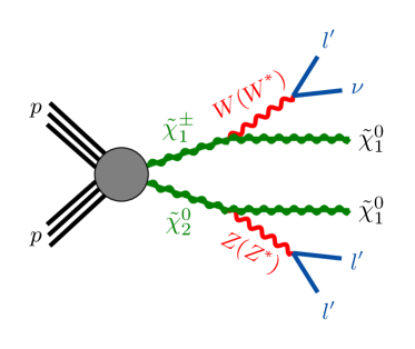
In this section, we study the effectiveness of various decision tree-based techniques for the search for direct pair production of charginos and neutralinos within the RPC MSSM scenario. To accomplish this, we consider a model where $M_{1}<M_{2}<<\mu$, ensuring that both the $\widetilde{\chi}_{1}^{\pm}$ and $\widetilde{\chi}_{2}^{0}$ exhibit wino-like characteristics and become mass degenerate, while the LSP ($\widetilde{\chi}_{1}^{0}$), remains predominantly bino-like. For such a scenario, the dominant production mode is $pp~{}\rightarrow~{}\widetilde{\chi}_{1}^{\pm}\widetilde{\chi}_{2}^{0}$, which gives rise to three lepton final state from subsequent decays as shown in Fig. 19.

Figure 19: The decays of the NLSP via real and virtual $W^{\pm}/Z$ bosons are displayed here.

We explore both the scenarios where both winos promptly decay to either on-shell or off-shell as follows:

• On-shell $WZ$ scenarios: the mass difference between the chargino ($\widetilde{\chi}_{1}^{\pm}$) or the second lightest neutralino ($\widetilde{\chi}_{2}^{0}$) and the lightest neutralino ($\widetilde{\chi}_{1}^{0}$) exceeds the $Z$ boson mass ($\Delta m(\widetilde{\chi}_{1}^{\pm}/\widetilde{\chi}_{2}^{0},\widetilde{\chi}_{1}^{0})>m_{Z}$), both $\widetilde{\chi}_{1}^{\pm}$ and $\widetilde{\chi}_{2}^{0}$ will undergo decays involving real $W$ and $Z$ bosons, such as $\widetilde{\chi}_{2}^{0}\rightarrow Z\widetilde{\chi}_{1}^{0}$ and $\widetilde{\chi}_{1}^{\pm}\rightarrow W^{\pm}\widetilde{\chi}_{1}^{0}$.

• Off-shell $WZ$ scenarios: In this case the mass difference between $\widetilde{\chi}_{1}^{\pm}/\widetilde{\chi}_{2}^{0}$ and $\widetilde{\chi}_{1}^{0}$ is less than $W$ boson mass ($\Delta m(\widetilde{\chi}_{1}^{\pm}/\widetilde{\chi}_{2}^{0},\widetilde{\chi}_{1}^{0})<m_{W}$) , $\widetilde{\chi}_{1}^{\pm}$ and $\widetilde{\chi}_{2}^{0}$ will undergo decay mediated by virtual bosons, such as $\widetilde{\chi}_{2}^{0}~{}\rightarrow~{}Z^{*}\widetilde{\chi}_{1}^{0}$ and $\widetilde{\chi}_{1}^{\pm}~{}\rightarrow~{}W^{\pm*}\widetilde{\chi}_{1}^{0}$. It may be noted that we have not considered the case where the mass gap is greater than $m_{W}$ and less than $m_{Z}$.

These $W/Z$ bosons decay into leptons with an equal branching fraction for each flavor ($l^{\prime}=e,\mu$, and $\tau$), resulting in a final state comprising precisely three light leptons ($l=e,\mu$) and missing energy coming from two LSPs. The decay processes for both real $WZ$ and virtual $W^{*}Z^{*}$ are depicted in Fig. 19. This $3l+\rm E{\!\!\!/}_{T}$ final state can originate from several Standard Model backgrounds such as $WZ$, $ZZ$, $t\bar{t}V$, $VVV$, $t\bar{t}$, and $Z+jets$. ATLAS has conducted a similar analysis using data from Run-I, Run-II, and high-luminosity LHC (HL-LHC). The current bounds on the electroweakinos from ATLAS Run-II results is 640 GeV for a massless $\widetilde{\chi}_{1}^{0}$ ATLAS:2021moa while the simulation by ATLAS indicated that future HL-LHC will be able to probe $\sim$ 1.1 TeV $\widetilde{\chi}_{1}^{\pm}/\widetilde{\chi}_{2}^{0}$ in such scenario with a cut-based analysis TheATLAScollaboration:2014nwe . Our aim is to study the sensitivity of wino searches using optimized cut-based and ML methods. Signal events are simulated using Pythia6 Sjostrand:2006za , while all background events are simulated using MadGraph5-aMC@NLO Alwall:2014hca at the leading order (LO). The NLO+NLL cross-sections for signals are calculated using Resummino-3.1.1 Fuks:2013vua , and the NLO cross-sections for all backgrounds are generated by MadGraph5-aMC@NLO which are listed in two Tables 7 and 8 in the Appendix 7. For this analysis, we consider a flat $k$ factor = 1.4 for all the SM backgrounds and SUSY signals. For the detector simulation, Delphes-3.5.0 deFavereau:2013fsa is utilized. Event reconstruction employs the anti-$k_{t}$ algorithm with a jet radius of 0.4, imposing criteria of $p_{T}>20$ and $|\eta|<2.8$ for jet selection. Leptons are identified with $p_{T}>10$ and $|\eta|<2.5~{}(2.7)$ for electrons (muons) respectively. For b-jets, $|\eta|<2.5$ is considered, with an 85% b-tagging efficiency and a 25% miss-tagging rate for light jets. Lepton-lepton isolation, lepton-jet isolation, etc, also have been implemented as described in the Refs. ATLAS:2021yyr ; Choudhury:2023eje .

Initially, a cut-based analysis is conducted, followed by machine learning (ML) analysis using various DT algorithms. Then, we look for the improvement in signal significance achieved through ML algorithms, along with a comparison of results from different ML approaches. Additionally, the impact of various hyperparameters such as learning rate ($\eta$) and number of trees is discussed. Furthermore, the significance of different kinematic features in discriminating signal and background events is illustrated using SHapley Additive ex-Planations (SHAP) values obtained through the SHAP package Shapley+1953+307+318 ; lundberg2018consistent ; pedregosa2018scikitlearn .
To do the further analysis, we choose four different benchmark points, allowed by LHC Run-II data, based on the mass difference between NLSP and LSP ($\Delta m(\widetilde{\chi}_{1}^{\pm}/\widetilde{\chi}_{2}^{0},\widetilde{\chi}_{1}^{0})$) with values $\Delta m(\widetilde{\chi}_{1}^{\pm}/\widetilde{\chi}_{2}^{0},\widetilde{\chi}_{1}^{0})=50,70$ and $>>m_{Z}$. The benchmark points are :
 Benchmark points           $m_{\widetilde{\chi}_{1}^{\pm}/\widetilde{\chi}_{2}^{0}}$ (GeV)             $m_{\widetilde{\chi}_{1}^{0}}$ (GeV)           $\Delta m$ (GeV)
         BP1                               400                            350                            50
            BP2                               500                            430                            70
            BP3                               800                            100                            700
            BP4                              1200                            100                           1000
                                              Pre-selection Cuts
 $N_{l}=3$           $\Delta R>0.3$           $N_{SFOS}\hskip 28.45274pt\geq 1$           $N_{\tau}=0$           $N_{b}=0$
  Pre-selection cuts: We select the events with exactly three leptons, which must have separation among them with $\Delta R>0.3$. Also, we choose the events with at least one same flavor opposite sign (SFOS) pair. We also impose that the events with no tau-jets and no b-tagged jets are selected for the analysis. After passing these selections with the remaining events, we do the cut-based analysis and ML analyses.

5.1 Cut-and-count analysis

Figure 20: The distribution of leading (top left) subleading (top middle) and third leading lepton (top right) transverse momenta and invariant mass of SFOS lepton pair, $m_{SFOS}$ (bottom left) transverse mass, $m_{T}$ (bottom middle) and missing energy, $\rm E{\!\!\!/}_{T}$ (bottom right) for three different signal benchmark points and three dominant backgrounds are displayed here. The cyan, light green, and light blue colored filled regions correspond to BP1, BP2 and BP3 respectively in each figure. Also, the red, blue and magenta colored lines refer to $WZ+jets$, $ZZ+jets$ and $t\bar{t}+jets$ respectively for every figure.

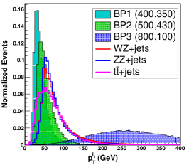
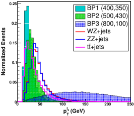
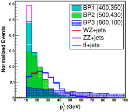
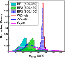
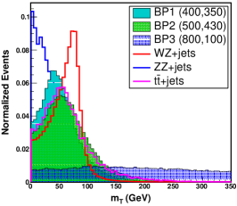
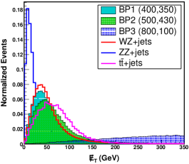
In this section, we investigate the search for wino-like $\widetilde{\chi}_{1}^{\pm}\widetilde{\chi}_{2}^{0}$ production at the HL-LHC with $\mathcal{L}$ = 3000 $fb^{-1}$ using the traditional cut-and-count method. We present the transverse momentum ($p_{T}$) distributions of the three chosen leptons, illustrated in upper panel of Fig. 20, for three distinct benchmark points (BP1, BP2, BP3) corresponding to $\Delta m=50,70$, and 700 GeV, alongside three prominent backgrounds: $WZ+jets$, $ZZ+jets$, and $t\bar{t}+jets$. The lepton $p_{T}$ distribution for signal and backgrounds are quite similar for the compressed benchmark points and distinct in the cases with large $\Delta m$. We identify the same-flavor opposite-sign (SFOS) lepton pair with mass closest to the $Z$ boson mass and exhibit the distribution of their invariant mass as $m_{SFOS}$, depicted in Fig. 20 (bottom left panel). The $m_{SFOS}$ distribution shows that the benchmark points $\Delta m>m_{Z}$ have a significant overlap with $WZ$ background while the compressed cases have peaked around $\Delta m=50$ and 70 GeV with a dominant overlap of $t\bar{t}$ background. Subsequently, we proceed to reconstruct the variable transverse mass, such as.

$$m_{T}=\sqrt{2p_{T}^{l_{w}}\rm E{\!\!\!/}_{T}(1-cos\Delta\phi)}$$ (19)

$l_{w}$ denotes the remaining third lepton subsequent to selecting a lepton pair for the reconstruction of the $Z$ boson, while $\Delta\phi$ signifies the angular disparity between the missing energy ($\rm E{\!\!\!/}_{T}$) and said third lepton. This parameter exploits the disparity between the distribution of the standard model background $WZ$, characterized by a Jacobian peak sharply diminishing around $m_{T}\sim m_{W}$. Additionally, the distributions of $\rm E{\!\!\!/}_{T}$ for both signals and backgrounds demonstrate that signal benchmark points generally possess larger missing energy compared to the standard model backgrounds. We have also defined another parameter as the ratio of the scalar sum of three leptons and the missing energy ($\gamma=\frac{\sum_{i}p_{T}^{l_{i}}}{\rm E{\!\!\!/}_{T}}$), which can discriminate the signal and backgrounds.

Selection	Signal region
Cuts	SR-A	SR-B	SR-C
$p_{T}^{l_{1,2,3}}$ (GeV)	$>$ 15, 10, 10	$>$ 20, 15, 15	$>$ 40, 30, 30
$m_{SFOS}$ (GeV)	10-50	30-70	81.2-101.2
$m_{T}$ (GeV)	$<$ 100	-	$>$ 140
$\rm E{\!\!\!/}_{T}$ (GeV)	$>$ 20	$>$ 15	$>$ 270
$N_{j}$	= 0	= 0	$\leq$ 1
$\gamma$	$>$ 1	$>$ 1	$>$ 0.6

Table 4: Signal regions with different selection cuts, optimized for separate signal points, are presented. SR-A and SR-B are optimized for BPs with $\Delta m=50$ and 70 GeV respectively. SR-C is optimized for large $\Delta m$ [(BP3 (800,100) and BP4 (1200,100)].

From the cut optimization, we have found that distinct sets of cuts become necessary for various benchmark points due to their varying $\Delta m$ values. For benchmark points with substantial $\Delta m$, cuts involving solely $p_{T}^{l_{1,2,3}}$, $m_{SFOS}$, $m_{T}$, $\rm E{\!\!\!/}_{T}$, number of jets ($N_{j}$) and $\gamma$ variables prove adequate. Here, the same cut set is effective for both the benchmark points with $\Delta m=700,1100$. Three different signal regions are defined in the Table 4 as SR-A, SR-B and SR-C corresponding to $\Delta m=50$ GeV, $\Delta m=70$ GeV and $\Delta m=700$ & 1100 GeV. We provide the signal yield, individual background yields, and total background yield, along with the signal significance without uncertainty ($\sigma_{ss}^{0}$) and with 10% ($\sigma_{ss}^{10}$) and 20% uncertainty ($\sigma_{ss}^{20}$) in Table 5. The signal significance without and with uncertainty are calculated using the formulas mentioned in the Equations. 9 and 10 (see section. 2). The $\sigma_{ss}^{0}$ ($\sigma_{ss}^{20}$) values corresponding to BP1, BP2, BP3, and BP4 are 4.72 (0.19), 2.04 (0.07), 10.77 (7.98), and 1.59 (1.30), respectively. The cut-based method shows that BP1, BP2 and BP3 are within reach of HL-LHC.

		SR-A	SR-B	SR-C
	$WZ+jets$	2247	4669	5.38
	$ZZ+jets$	187	301	2.93
Backgrounds	$t\bar{t}+jets$	13198	13176	0.00
	$VVV+jets$	116	218	1.69
	$t\bar{t}V+jets$	37	88	0.47
	$Z+jets$	0.00	0.00	0.00
	Total	15785	18454	10.47	Signal Significance
	Background yield				$\sigma_{ss}^{0}$	$\sigma_{ss}^{10}$	$\sigma_{ss}^{20}$
	BP1	596	-	-	4.72	0.37	0.19
Signal	BP2	-	277	-	2.04	0.15	0.07
	BP3	-	-	51.10	10.77	9.76	7.98
	BP4	-	-	5.55	1.59	1.50	1.30

Table 5: The different background yield, total background yield and signal yields calculated at $\sqrt{s}=14$ TeV and $\mathcal{L}=3000~{}fb^{-1}$ corresponding to different signal regions are shown in this table. The signal significance without uncertainty ($\sigma_{ss}^{0}$), with 10% ($\sigma_{ss}^{10}$) and 20% systematic uncertainty ($\sigma_{ss}^{20}$) are also presented in the last three column.

5.2 Machine Learning based analysis

We will now conduct a similar analysis employing Machine Learning algorithms. For this purpose, we have compiled a dataset comprising events after the pre-selection cuts. In order to fully harness the benefits of utilizing a boosted decision tree approach over the cut-and-count method for distinguishing signal from background, it’s crucial to incorporate not just the primary kinematic variables such as the number of leptons ($n_{l}$), number of jets ($n_{j}$), and transverse momenta of leptons ($p_{T}^{l}$), but also to generate additional derived variables like the mass of same-flavor opposite-sign (SFOS) pairs, the sum of transverse momenta ($p_{T}$) of leptons and jets, as well as variables such as effective mass. Therefore, we have developed 21 distinct features tailored for the specific analysis required in machine learning. These features variables are mentioned below :

• The transverse momenta of the three chosen leptons, denoted as $p_{T}^{l_{1}}$, $p_{T}^{l_{2}}$, and $p_{T}^{l_{3}}$, are represented by three variables.

• The angular difference between each pair of the three leptons, denoted as $\Delta R_{l_{1}l_{2}}$, $\Delta R_{l_{1}l_{3}}$, and $\Delta R_{l_{2}l_{3}}$ (three features), is measured. (3 features)

• Azimuthal angular difference between leptons and missing energy represented as $\Delta\phi_{l_{i}\rm E{\!\!\!/}_{T}}$ where i=1,2,3 (3 features)

• No of jets, $N_{j}$ and missing energy, $\rm E{\!\!\!/}_{T}$ (2 features)

• The SFOS pair number ($N_{SFOS}$) and the mass of SFOS pair ($m_{SFOS}$) with mass closest of $Z$ boson mass (2 features)

• After selecting the SFOS pair, with the remaining lepton, we construct the transverse mass ($m_{T}$), which is defined in Equation. 19. Also, we calculate the invariant mass of three leptons ($m_{3l}$). Then we calculate the difference between the masses of $m_{3l}$ and $m_{SFOS}$ denoted as $\Delta m(m_{3l},m_{SFOS})$. (3 features)

• Next, we compute the scalar sum of the transverse momenta of three leptons ($H_{T}^{lep}$) and the scalar sum of transverse momenta of jets ($H_{T}^{jet}$). Additionally, we determine the sum of missing energy and $H_{T}^{lep}$ as $H_{T}^{lep}+\rm E{\!\!\!/}_{T}$, and similarly for jets as $H_{T}^{jet}+\rm E{\!\!\!/}_{T}$. We introduce the effective mass variable, defined as $m_{eff}=H_{T}^{lep}+H_{T}^{jet}+\rm E{\!\!\!/}_{T}$, comprising a total of 5 features.

We incorporate the relevant weight into both the signal and background during the preparation of the data file. Subsequently, we proceed with the machine learning analysis using four distinct algorithms.

5.2.1 Hyperparameter variation for different algorithms

In this section we present the role of hyperparameters for the performances of different algorithms. In Sec. 4, we have already summarized the mechanics of these algorithms. Each algorithm offers a range of hyperparameters for customization. For instance, with the XGBoost algorithm, one can adjust parameters such as the learning rate ($\eta$), the number of trees, the maximum depth of each tree ($max\_depth$), the minimum weight required for node splitting (Min. child weight), a regularization parameter ($\gamma$) to prevent overfitting, an $\alpha$ parameter for further regularization via a penalty term within the loss function, and the subsample size of the dataset used for training, which is randomly selected etc..

Figure 21: The signal significance as a function of learning rate ($\eta$), number of trees or estimators and the number of training events for the BP3 (800,100) signal benchmark point are displayed corresponding to the four different ML algorithms in the left, middle and right panel respectively.

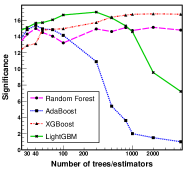
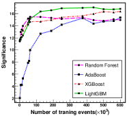
Similarly, the LightGBM algorithm shares many of these hyperparameters, alongside additional parameters like the number of leaves, which should be set to a value less than $2^{max\_depth}$ to mitigate overfitting and enhance model accuracy. AdaBoost follows a similar optimization strategy, with parameters such as the number of estimators, which corresponds to the number of trees. However, unlike other algorithms, Random Forest doesn’t include a learning rate parameter in its optimization process.

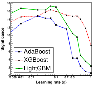
We have estimated the best set of hyperparameters effective for each algorithm and mentioned in the Table. 9 (see Appendix. 7). Upon determining the optimal hyperparameters for each algorithm, we investigate how varying the learning rate parameter affects the signal significance across three algorithms: AdaBoost, XGBoost, and LightGBM. We examine the range of the $\eta$ parameter from 0.0001 to 1.0 and depict the resulting variations in Fig. 21 (left). The plot clearly indicates that AdaBoost demonstrates peak performance around $\eta$ = 0.02-0.08, XGBoost performs optimally within $\eta$ = 0.05-0.15, and LightGBM shows higher significance around $\eta$ = 0.01-0.1.

Additionally, we explore the impact of the number of trees, ranging from 1 to 5000, on the algorithms, as shown in Fig. 21 (middle), while keeping all other parameters constant. It becomes evident from the plot that for Random Forest and XGBoost algorithms, the signal significance reaches its maximum after approximately 300 trees, with minimal variation thereafter. However, for AdaBoost and LightGBM algorithms, the signal significance declines rapidly after 100 and 500 trees, respectively. Furthermore, we analyze the effect of the number of training events in the dataset on all algorithms, presented in Fig. 21 (right), to ensure that we have taken an adequate amount of data for the ML analysis. Upon reaching around 3$\times 10^{5}$ training events, all algorithms achieve maximum significance, with marginal variation as the number of training events increases.

5.2.2 Feature importance with SHapley

As discussed in Sec.5.2, for this analysis, more than 20 distinct features have been used to train the ML model and the impact of these features in discriminating the signal and background can be determined using SHAP package Shapley+1953+307+318 ; lundberg2018consistent ; pedregosa2018scikitlearn . In the context of tree ensemble methods like gradient boosting methods or random forests, it is common to assign importance values to each input feature in order to comprehend the predictions. These values can be calculated for an individualized prediction or the global prediction of an entire dataset. Popular packages like XGBoost Shapley+1953+307+318 ; lundberg2018consistent ; pedregosa2018scikitlearn offer implementations of tree ensembles that enable users to calculate a metric of feature importance. These metrics aim to condense the complexity of ensemble models and offer an understanding of the key features influencing the model’s predictions. Global feature importance is derived through three main methodologies gain, split count, permutation and Saabas method. However, most of these methods of calculating feature importance metrics are inconsistent and ineffective.
However, SHapley values, which stem from principles of game theory, demonstrate the contribution of an individual player within a group. As indicated in Ref. lundberg2018consistent , among various techniques mentioned above, SHapley values emerge as the most dependable measure for selecting feature importance. This method of local feature attribution, founded on SHapley values, was pioneered by S. Lundberg and S. Lee, as outlined in lundberg2017unified . The technique of calculating SHapley values involves training the model on various subsets of features, where each subset is a subset of the full feature set. It assigns an importance score to each feature, indicating its impact on model predictions when included. To calculate this impact, two models are trained: one with the feature in the model and another without it. The difference in predictions between these models, considering the current input, helps quantify the feature’s influence. Since the influence of a feature’s absence is influenced by other features in the model, these differences are computed across all possible feature subsets, excluding the feature under consideration. Subsequently, SHapley values are computed and utilized to attribute importance to each feature. The formula used for the calculation of SHapley value looks like lundberg2018consistent

$$\phi_{i}=\sum_{S\subseteq N\setminus\{i\}}\frac{|S|!(M-|S|-1)!}{M!}[f_{x}(S\cup\{i\})-f_{x}(S)]$$ (20)

Figure 22: Left: SHAP summary plot for then signal point BP3 (800,100)
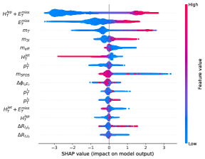
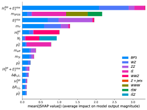
Right: SHAP summary bar plot for BP3 and all the backgrounds. The most important 15 feature variables are displayed here.

In this context, N denotes the complete set of features and “i” represents the feature under consideration for SHapley value calculation. M signifies the overall count of features. S denotes a subset of N that excludes i. The function $f_{x}$ represents the model’s prediction. Consequently, the algorithm evaluates a weighted sum of the variances in model predictions when including or excluding the ith feature across all potential combinations of the subset S.
Various kinds of visualizations can be generated using SHapley values to illustrate how different features impact the model. SHAP summary plots utilize individualized feature attributions to encapsulate the significance of each feature effectively while maintaining visual simplicity. Initially, features are arranged based on their overall impact, represented by the sum of absolute SHapley values. Subsequently, the corresponding SHapley values are horizontally plotted, with stacking occurring vertically if space becomes insufficient. The SHAP summary plot (dotted) is shown in the Fig. 22. Every point is shaded according to the corresponding feature’s value, ranging from a low (blue) hue to a high (red) one. Also, we consider the absolute SHapley values and show a bar-type summary plot where each color represents each class and the bar width shows the effect of each feature on classifying each class. In the left panel of the Fig. 22, we have displayed the SHapley value distribution for the signal benchmark point BP3 only. The right panel of Fig. 22 represents the combined effect of the signal point and all SM backgrounds. In Fig. 22, we plot only the first 15 feature variables according to importance. The variable ($H_{T}^{lep}+\rm E{\!\!\!/}_{T}$) is the top most important feature, while the $m_{SFOS}$ variable is the next effective variable when the model tries to discriminate the signal and background (see the right panel of Fig. 22. and the combined effect of the signal and all the background (right). It is obvious that when we try to discriminate the signal and background, variable $m_{SFOS}$ will be very effective and that’s why it has more importance value in the bar plot (right) than the dotted plot (left). The other variables like $\rm E{\!\!\!/}_{T}$ and $m_{T}$ show the higher SHapley value, which is quite similar to the cut-based analysis.

5.2.3 Comparison of results coming from different algorithms

Figure 23: The signal and background events distribution as a function of the predicted probability in the test dataset corresponding to the BP3 for the Random Forest classifier (upper left), AdaBoost (upper right), XGBoost classifier (lower left) and LightGBM (lower right).

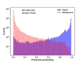
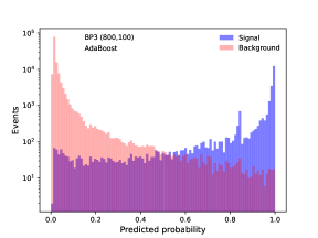
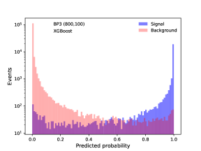
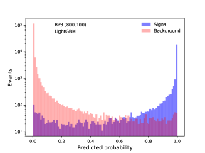
After optimization of hyperparameters for each algorithm, we proceed to visualize the distribution of signal and background events corresponding to two signal benchmark points BP1 and BP3, which represent two different scenarios like small $\Delta m$ (50 GeV) and large $\Delta m$ (700 GeV). The event distributions of BP3 (BP1) are displayed in Fig. 23 (Fig.. 25 in the Appendix. 7). Analysis of the distributions corresponding to BP3 reveals that the XGBoost and LightGBM algorithms outperform Random Forest and AdaBoost in discriminating signal from background, as evidenced by the higher number of background events at larger probability cuts for the latter two algorithms. For small $\Delta m$ also, these two algorithms work better, but for all the algorithms, there is significant overlapping between signal and background which is evident from the Fig. 25. In the Fig. 20, the distribution of the kinematic variables also displays the same behavior about the significant overlapping.

We also represent the ROC curve for two different benchmark points BP1 (left) and BP3 (right) in the Figure. 24. Here we can see that auc values are a little bit different for each algorithm corresponding to BP1 whereas for BP3, the auc values are pretty close.

Figure 24: ROC curves and auc values are shown for each ML algorithm corresponding to two signal benchmark points BP1 (left) and BP3 (right) are displayed here.

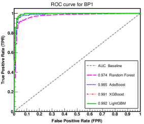
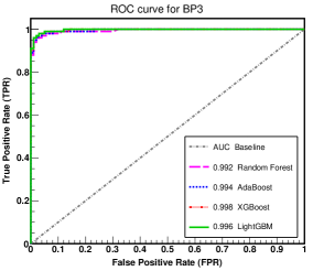
	BP1 (400,350)						BP2 (500,430)
Algorithm	Proba-	Signal	Back-	$\sigma_{ss}^{0}$	$\sigma_{ss}^{10}$	$\sigma_{ss}^{20}$	Proba	Signal	Back-	$\sigma_{ss}^{0}$	$\sigma_{ss}^{10}$	$\sigma_{ss}^{20}$
	bility	yield	ground				bility	yield	ground
	cut	(S)	yield (B)				cut	(S)	yield (B)
RF	0.80	1152	5772	14.70	1.86	0.94	0.70	559	12158	5.03	0.45	0.23
AdaBoost	0.86	1439	6434	17.22	2.05	1.03	0.80	760	13276	6.54	0.56	0.28
XGBoost	0.92	1264	3757	19.61	3.01	1.52	0.83	786	10017	7.76	0.76	0.38
LightGBM	0.92	1254	3512	20.06	3.18	1.60	0.90	572	4996	7.96	1.09	0.55
	BP3 (800,100)						BP4 (1200,100)
RF	0.96	81.28	11.94	14.85	13.12	10.40	0.92	9.43	11.99	2.45	2.29	1.94
AdaBoost	0.98	77.12	12.19	14.20	12.56	9.95	0.98	9.49	17.91	2.08	1.89	1.54
XGBoost	0.99	93.78	12.38	16.39	14.35	11.27	0.99	10.24	12.05	2.63	2.45	2.08
LightGBM	0.99	99.64	11.94	17.30	15.14	11.90	0.97	10.05	11.97	2.60	2.42	2.06

Table 6: The signal yields and the total background yields calculated at $\sqrt{s}=14$ TeV and $\mathcal{L}=3000~{}fb^{-1}$ corresponding to the four benchmark points are presented here for four different DT algorithms. We also show the signal significance with 0% ($\sigma_{ss}^{0}$), 10% ($\sigma_{ss}^{10}$) and 20% ($\sigma_{ss}^{20}$) systematic uncertainty. Here RF refers to the Random Forest algorithm.

In the Table. 6 we provide the signal yield, total background yield, and signal significance without systematic uncertainty ($\sigma_{ss}^{0}$), and with uncertainties of 10% ($\sigma_{ss}^{10}$) and 20% ($\sigma_{ss}^{20}$). For benchmark points with low $\Delta m$ (BP1 abd BP2), there are significant overlap between signal and background events and the dominant contribution comes from $WZ+jets$ and $t\bar{t}+jets$ backgrounds. In these compressed scenarios, due to the small $S/B$ ratio ($<1$), we observe a sharp decrease in the significance when we consider the systematic uncertainties. For BP1 and BP2, the signal significance becomes $\sim$ 3-4 times larger as compared to the cut-and-count method. For BP3 and BP4, the signal significance increases by $\sim$ 30-60% in ML method. Specifically, when considering signal significance with uncertainty, we can exclude the point where $m_{\widetilde{\chi}_{1}^{\pm}/\widetilde{\chi}_{2}^{0}}$ = 400 GeV for $m_{\widetilde{\chi}_{1}^{0}}$ = 350 GeV. Similarly, we can also exclude $m_{\widetilde{\chi}_{1}^{\pm}/\widetilde{\chi}_{2}^{0}}$ = 1200 GeV for $m_{\widetilde{\chi}_{1}^{0}}$ = 100 GeV, regardless of uncertainty. It should be noted that the performances of XGBoost and LightGBM are almost similar and LightGBM gives a slightly better signal significance. The Table. 6 indicates that even with 20% systematic uncertainty chargino mass with 800 (1200) GeV will be within $\sim 12\sigma$ and $\sim 2\sigma$ reach for a LSP mass of 100 GeV.

6 Summary

Over the years, machine laerning techniques have significantly boosted efficiency and accuracy in HEP data analysis for both experimental and phenomenological works. For the analyses of event triggering, jet tagging, particle identification, event selection, object reconstruction, event classification etc., the HEP community has been widely using the boosted decision tree (BDT) algorithms for a long time. We have briefly summarized the major important analyses performed by the ATLAS and CMS collaboration utilizing LHC data as well as the works of the phenomenological groups involving the use of ML algorithms with emphasis on DT-based approaches. We have also outlined the basic concepts of machine learning along with different kinds of loss functions and their roles, issues of underfitting, overfitting, etc. Evaluation of the effectiveness and accuracy of the ML models in solving a specific task, e.g., classifying signal and background events, can be done using performance metrics. Different kinds of metrics relevant to particle physics analysis, like ROC curve, F-score, ams score, etc., are discussed in detail.

In this article, we have focused solely on a prominent machine learning technique, namely Decision Tree (DT), specifically boosted decision tree, which is primarily used for tasks in supervised classification and regression. We particularly explore four decision tree-based ML algorithms, namely, Random Forest, AdaBoost and two gradient boosting frameworks such as XGBoost, and LightGBM, in the context of Supersymmetry which is a well-promising candidate for beyond the Standard model framework. We summarize the basic concepts and working principles of these four algorithms along with the flowcharts. In numerous analyses, both the ATLAS and CMS collaborations, HEP phenomenological groups have employed BDT algorithms to enhance the sensitivity of sparticle searches within the framework of RPC and RPV SUSY models. However, exploring the compressed SUSY parameter space still reamsins as a significant challenge.

Using an example of wino type electroweakino productions at the high luminosity LHC, we demonstrate how these algorithms lead to improvement in the search sensitivity compared to traditional cut-based methods in both compressed and non-compressed R-Parity conserving SUSY scenarios. The optimization of hyperparameters and its role in signal significance are studied in detail for these four algorithms. We have also discussed how to find out the individualized and global feature importance in ML methods using SHAP package. We have found that there are $\sim$ 30-60% gains in the significance for the signal benchmark points with a large mass gap between NLSP-LSP pair, whereas, for the compressed region (mass gap 50 and 70 GeV), the signal significance improves by $\sim$ 3-4 times compared to the cut-based analysis. We have obtained that the LightGBM and XGBoost algorithms perform better than the other two algorithms Random Forest and AdaBoost. Although the deep neural networks (DNN) or deep learning (DL) techniques, which are based on multilayer NN, are gaining popularity, BDTs continue to be highly relevant and important in High Energy Physics due to their user-friendly nature, interpretability, computational efficiency, and more.

Acknowledgments: Authors would like to thank Ritik Pal for fruitful suggestions. The work of A.C is supported by the SERB Core Research Grant CRG/2023/008570.

Data availability statement: No data associated in the manuscript.

7 Appendix

Benchmark point	Cross-section, $\sigma$ (fb)	$\sigma^{\prime}=\sigma\times 3l^{\prime}$ (fb)
BP1(400,350)	144.26	4.76
BP2(500,430)	56.42	1.86
BP3(800,100)	6.19	0.20
BP4(1200,100)	0.6	0.02

Table 7: The NLL+NLO cross-section of the signal benchmark points are listed in this table.

Background	Cross-section, $\sigma$ (fb)	$\sigma^{\prime}=\sigma\times nl^{\prime}$ (fb)	Total event generated
$WZ+jets$	$3.619\times 10^{4}$	1196 ($n=3$)	3.7$\times 10^{6}$
$ZZ+jets$	$1.067\times 10^{4}$	111 ($n=4$)	1.6$\times 10^{5}$
$t\bar{t}+jets$	$5.930\times 10^{5}$	62250 ($n=2$)	1.2$\times 10^{7}$
$WWZ+jets$	$1.488\times 10^{2}$	3.3251 ($n=3$)	9.8$\times 10^{4}$
$WWW+jets$	$1.925\times 10^{2}$	6.546 ($n=3$)	5.3$\times 10^{4}$
$t\bar{t}W+jets$	$5.510\times 10^{2}$	18.74 ($n=3$)	1.6$\times 10^{5}$
$t\bar{t}Z+jets$	$6.893\times 10^{2}$	15.4 ($n=3$)	1.3$\times 10^{5}$
$Z+jets$	$4.516\times 10^{7}$	4606000 ($n=2$)	1.3$\times 10^{6}$

Table 8: The matched cross-sections and the total event generated corresponding to each SM background are displayed in this table.

Figure 25: The signal and background events distribution with the probability cut in the test dataset corresponding to the BP1 for the Random Forest classifier (upper left), AdaBoost (upper right), XGBoost classifier (lower left) and LightGBM (lower right).

Figure 26: The distributions of the signal significance with the probability cut are shown for all the benchmark points corresponding to each different algorithm.

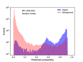
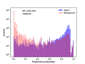
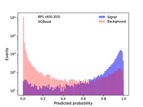
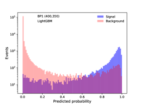
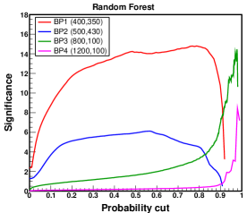
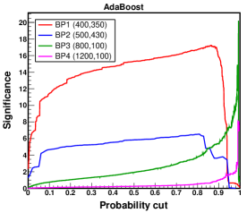
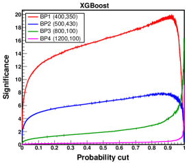
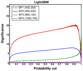
Optimized hyperparameters
Random Forest	AdaBoost	XGBoost	LightGBM
n_estimators = 300	n_estimators = 30	num_trees = 500	boosting_type = ‘gbdt’
max_depth = 5	max_depth = 6	max_depth = 8	num_leaves = 70
max_leaf_nodes = 150	learning_rate = 0.03	learning_rate = 0.07	max_depth = 8
max_features = ‘sqrt’	algorithm=“SAMME.R”	subsample = 0.5	learning_rate = 0.1
criterion = ‘gini’		min_child_weight = 2.5	n_estimators = 200
		alpha = 0.21	subsample = 0.5
		gamma = 0.68	min_child_weight = 1.5
			colsample_bytree = 0.8

Table 9: The values of optimized hyperparameters that lead to the best performance of the model corresponding to different algorithms are mentioned in this table.

References

- (1) S. P. Martin, A Supersymmetry primer, Adv. Ser. Direct. High Energy Phys. 18 (1998) 1–98, [hep-ph/9709356].
- (2) M. Drees, P. Roy and R. Godbole, Theory and Phenomenology of Sparticles: An Account of Four-dimensional N. World Scientific, 2004.
- (3) H. Baer and X. Tata, Weak Scale Supersymmetry: From Superfields to Scattering Events. Cambridge University Press, 2006.
- (4) “Atlas susy public result.” https://twiki.cern.ch/twiki/bin/view/AtlasPublic/SupersymmetryPublicResults.
- (5) “Cms susy public result.” https://cms-results.web.cern.ch/cms-results/public-results/preliminary-results/SUS/index.html.
- (6) B. Bhattacherjee, A. Choudhury, K. Ghosh and S. Poddar, Compressed supersymmetry at 14 TeV LHC, Phys. Rev. D 89 (2014) 037702, [1308.1526].
- (7) J. Dutta, P. Konar, S. Mondal, B. Mukhopadhyaya and S. K. Rai, A Revisit to a Compressed Supersymmetric Spectrum with 125 GeV Higgs, JHEP 01 (2016) 051, [1511.09284].
- (8) M. Chakraborti, U. Chattopadhyay and S. Poddar, How light a higgsino or a wino dark matter can become in a compressed scenario of MSSM, JHEP 09 (2017) 064, [1702.03954].
- (9) D. Chowdhury, K. M. Patel, X. Tata and S. K. Vempati, Indirect Searches of the Degenerate MSSM, Phys. Rev. D 95 (2017) 075025, [1612.06471].
- (10) J. Dutta, P. Konar, S. Mondal, B. Mukhopadhyaya and S. K. Rai, Search for a compressed supersymmetric spectrum with a light Gravitino, JHEP 09 (2017) 026, [1704.04617].
- (11) R. Kumar Barman, G. Belanger and R. M. Godbole, Status of low mass LSP in SUSY, Eur. Phys. J. ST 229 (2020) 3159–3185, [2010.11674].
- (12) R. K. Barman, G. Bélanger, B. Bhattacherjee, R. M. Godbole and R. Sengupta, Is Light Neutralino Thermal Dark Matter in the Phenomenological Minimal Supersymmetric Standard Model Ruled Out?, Phys. Rev. Lett. 131 (2023) 011802, [2207.06238].
- (13) Y. He, L. Meng, Y. Yue and D. Zhang, Impact of the recent measurement of (g-2), the LHC search for supersymmetry, and the LZ experiment on the minimal supersymmetric standard model, Phys. Rev. D 108 (2023) 115010, [2303.02360].
- (14) M. Chakraborti, U. Chattopadhyay, A. Choudhury, A. Datta and S. Poddar, Reduced LHC constraints for higgsino-like heavier electroweakinos, JHEP 11 (2015) 050, [1507.01395].
- (15) M. Chakraborti, U. Chattopadhyay, A. Choudhury, A. Datta and S. Poddar, The Electroweak Sector of the pMSSM in the Light of LHC - 8 TeV and Other Data, JHEP 07 (2014) 019, [1404.4841].
- (16) N. Bhattacharyya, A. Choudhury and A. Datta, Low mass neutralino dark matter in mSUGRA and more general models in the light of LHC data, Phys. Rev. D 84 (2011) 095006, [1107.1997].
- (17) A. Choudhury and A. Datta, Many faces of low mass neutralino dark matter in the unconstrained MSSM, LHC data and new signals, JHEP 06 (2012) 006, [1203.4106].
- (18) H. Baer, V. Barger and H. Serce, Anomalous muon magnetic moment, supersymmetry, naturalness, LHC search limits and the landscape, Phys. Lett. B 820 (2021) 136480, [2104.07597].
- (19) M. Chakraborti, S. Iwamoto, J. S. Kim, R. Masełek and K. Sakurai, Supersymmetric explanation of the muon g – 2 anomaly with and without stable neutralino, JHEP 08 (2022) 124, [2202.12928].
- (20) P. Athron, C. Balazs, D. H. J. Jacob, W. Kotlarski, D. Stockinger and H. Stockinger-Kim, New physics explanations of aμ in light of the FNAL muon g - 2 measurement, JHEP 09 (2021) 080, [2104.03691].
- (21) M. Endo, K. Hamaguchi, S. Iwamoto and T. Kitahara, Supersymmetric interpretation of the muon g – 2 anomaly, JHEP 07 (2021) 075, [2104.03217].
- (22) M. Chakraborti, L. Roszkowski and S. Trojanowski, GUT-constrained supersymmetry and dark matter in light of the new determination, JHEP 05 (2021) 252, [2104.04458].
- (23) A. Choudhury, S. Rao and L. Roszkowski, Impact of LHC data on muon solutions in a vectorlike extension of the constrained MSSM, Phys. Rev. D 96 (2017) 075046, [1708.05675].
- (24) A. Choudhury, L. Darme, L. Roszkowski, E. M. Sessolo and S. Trojanowski, Muon g 2 and related phenomenology in constrained vector-like extensions of the MSSM, JHEP 05 (2017) 072, [1701.08778].
- (25) H. Banerjee, P. Byakti and S. Roy, Supersymmetric gauged U(1) model for neutrinos and the muon anomaly, Phys. Rev. D 98 (2018) 075022, [1805.04415].
- (26) H. Banerjee, B. Dutta and S. Roy, Supersymmetric gauged model for electron and muon anomaly, JHEP 03 (2021) 211, [2011.05083].
- (27) M. Chakraborti, S. Heinemeyer and I. Saha, The new “MUON G-2” result and supersymmetry, Eur. Phys. J. C 81 (2021) 1114, [2104.03287].
- (28) M. Frank, Y. Hicylmaz, S. Mondal, O. Ozdal and C. S. Un, Electron and muon magnetic moments and implications for dark matter and model characterisation in non-universal U(1) supersymmetric models, JHEP 10 (2021) 063, [2107.04116].
- (29) M. I. Ali, M. Chakraborti, U. Chattopadhyay and S. Mukherjee, Muon and electron anomalies with non-holomorphic interactions in MSSM, Eur. Phys. J. C 83 (2023) 60, [2112.09867].
- (30) K. Kowalska, L. Roszkowski, E. M. Sessolo and A. J. Williams, GUT-inspired SUSY and the muon g 2 anomaly: prospects for LHC 14 TeV, JHEP 06 (2015) 020, [1503.08219].
- (31) J. Chakrabortty, A. Choudhury and S. Mondal, Non-universal Gaugino mass models under the lamppost of muon (g-2), JHEP 07 (2015) 038, [1503.08703].
- (32) A. Choudhury and S. Mondal, Revisiting the Exclusion Limits from Direct Chargino-Neutralino Production at the LHC, Phys. Rev. D 94 (2016) 055024, [1603.05502].
- (33) A. L. Samuel, Some Studies in Machine Learning Using the Game of Checkers. I, pp. 335–365. Springer New York, New York, NY, 1988. 10.1007/978-1-4613-8716-9_14.
- (34) CDF collaboration, T. Aaltonen et al., Observation of Single Top Quark Production and Measurement of —— with CDF, Phys. Rev. D 82 (2010) 112005, [1004.1181].
- (35) D0 collaboration, V. M. Abazov et al., Evidence for production of single top quarks, Phys. Rev. D 78 (2008) 012005, [0803.0739].
- (36) D0 collaboration, V. M. Abazov et al., Evidence for production of single top quarks and first direct measurement of —Vtb—, Phys. Rev. Lett. 98 (2007) 181802, [hep-ex/0612052].
- (37) CMS collaboration, V. Khachatryan et al., Observation of the Diphoton Decay of the Higgs Boson and Measurement of Its Properties, Eur. Phys. J. C 74 (2014) 3076, [1407.0558].
- (38) TMVA collaboration, A. Hocker et al., TMVA - Toolkit for Multivariate Data Analysis, physics/0703039.
- (39) T. Chen and C. Guestrin, XGBoost: A Scalable Tree Boosting System, 1603.02754.
- (40) Preface to special issue on “learning to discover”, International Journal of Modern Physics A 35 (2020) 2002003, [https://doi.org/10.1142/S0217751X20020030].
- (41) G. H. Y. LeCun, Y. Bengio, Deep Learning, .
- (42) P. C. Bhat, Multivariate Analysis Methods in Particle Physics, Ann. Rev. Nucl. Part. Sci. 61 (2011) 281–309.
- (43) D. Guest, K. Cranmer and D. Whiteson, Deep Learning and its Application to LHC Physics, Ann. Rev. Nucl. Part. Sci. 68 (2018) 161–181, [1806.11484].
- (44) D. Bourilkov, Machine and Deep Learning Applications in Particle Physics, Int. J. Mod. Phys. A 34 (2020) 1930019, [1912.08245].
- (45) M. D. Schwartz, Modern Machine Learning and Particle Physics, 2103.12226.
- (46) G. Carleo, I. Cirac, K. Cranmer, L. Daudet, M. Schuld, N. Tishby et al., Machine learning and the physical sciences, Rev. Mod. Phys. 91 (2019) 045002, [1903.10563].
- (47) J. Shlomi, P. Battaglia and J.-R. Vlimant, Graph Neural Networks in Particle Physics, 2007.13681.
- (48) M. Abdughani, J. Ren, L. Wu, J. M. Yang and J. Zhao, Supervised deep learning in high energy phenomenology: a mini review, Commun. Theor. Phys. 71 (2019) 955, [1905.06047].
- (49) A. S. Cornell, W. Doorsamy, B. Fuks, G. Harmsen and L. Mason, Boosted decision trees in the era of new physics: a smuon analysis case study, JHEP 04 (2022) 015, [2109.11815].
- (50) Y. Coadou, Boosted decision trees, 2206.09645.
- (51) C. Bishop, Pattern Recognition and Machine Learning, vol. 16, pp. 140–155. 01, 2006. 10.1117/1.2819119.
- (52) T. Hastie, R. Tibshirani, J. H. Friedman and J. H. Friedman, The elements of statistical learning: data mining, inference, and prediction, vol. 2. Springer, 2009.
- (53) J. G. Carbonell, R. S. Michalski and T. M. Mitchell, An overview of machine learning, Machine learning (1983) 3–23.
- (54) J. Bardhan, T. Mandal, S. Mitra, C. Neeraj and M. Patra, Unsupervised and lightly supervised learning in particle physics, 2403.13676.
- (55) M. Niazkar, A. Menapace, B. Brentan, R. Piraei, D. Jimenez, P. Dhawan et al., Applications of xgboost in water resources engineering: A systematic literature review (dec 2018 – may 2023), Environmental Modelling & Software 174 (02, 2024) 105971.
- (56) C. Bentéjac, A. Csörgő and G. Martínez-Muñoz, A comparative analysis of gradient boosting algorithms, Artificial Intelligence Review 54 (2021) 1937–1967.
- (57) G. M. Weiss and F. Provost, Learning when training data are costly: The effect of class distribution on tree induction, Journal of artificial intelligence research 19 (2003) 315–354.
- (58) N. V. Chawla, Data Mining for Imbalanced Datasets: An Overview, pp. 853–867. Springer US, Boston, MA, 2005. 10.1007/0-387-25465-X_40.
- (59) M. Hossin and S. M.N, A review on evaluation metrics for data classification evaluations, International Journal of Data Mining & Knowledge Management Process 5 (03, 2015) 01–11.
- (60) T. Saito and M. Rehmsmeier, The precision-recall plot is more informative than the roc plot when evaluating binary classifiers on imbalanced datasets, PLoS One 10 (2015) .
- (61) A. Luque, A. Carrasco, A. Martín and A. de las Heras, The impact of class imbalance in classification performance metrics based on the binary confusion matrix, Pattern Recognition 91 (2019) 216–231.
- (62) Q. Gu, L. Zhu and Z. Cai, Evaluation measures of the classification performance of imbalanced data sets, in Computational Intelligence and Intelligent Systems (Z. Cai, Z. Li, Z. Kang and Y. Liu, eds.), (Berlin, Heidelberg), pp. 461–471, Springer Berlin Heidelberg, 2009.
- (63) G. Cowan, Discovery sensitivity for a counting experiment with background uncertainty, 2012.
- (64) G. Cowan, K. Cranmer, E. Gross and O. Vitells, Asymptotic formulae for likelihood-based tests of new physics, Eur. Phys. J. C 71 (2011) 1554, [1007.1727].
- (65) HEP ML Community, “A Living Review of Machine Learning for Particle Physics.”
- (66) B. P. Roe, H.-J. Yang, J. Zhu, Y. Liu, I. Stancu and G. McGregor, Boosted decision trees as an alternative to artificial neural networks for particle identification, Nuclear Instruments and Methods in Physics Research Section A: Accelerators, Spectrometers, Detectors and Associated Equipment 543 (2005) 577–584.
- (67) H.-J. Yang, B. P. Roe and J. Zhu, Studies of boosted decision trees for miniboone particle identification, Nuclear Instruments and Methods in Physics Research Section A: Accelerators, Spectrometers, Detectors and Associated Equipment 555 (2005) 370–385.
- (68) Y. Freund and R. E. Schapire, A decision-theoretic generalization of on-line learning and an application to boosting, Journal of Computer and System Sciences 55 (1997) 119–139.
- (69) CMS collaboration, D. Acosta et al., Boosted Decision Trees in the Level-1 Muon Endcap Trigger at CMS, J. Phys. Conf. Ser. 1085 (2018) 042042.
- (70) CMS collaboration, A. Zabi, J. W. Berryhill, E. Perez and A. D. Tapper, The Phase-2 Upgrade of the CMS Level-1 Trigger, .
- (71) V. V. Gligorov and M. Williams, Efficient, reliable and fast high-level triggering using a bonsai boosted decision tree, JINST 8 (2013) P02013, [1210.6861].
- (72) T. Likhomanenko, P. Ilten, E. Khairullin, A. Rogozhnikov, A. Ustyuzhanin and M. Williams, LHCb Topological Trigger Reoptimization, J. Phys. Conf. Ser. 664 (2015) 082025, [1510.00572].
- (73) B. Bhattacherjee, P. Konar, V. S. Ngairangbam and P. Solanki, LLPNet: Graph Autoencoder for Triggering Light Long-Lived Particles at HL-LHC, 2308.13611.
- (74) J. Bendavid, Efficient Monte Carlo Integration Using Boosted Decision Trees and Generative Deep Neural Networks, 1707.00028.
- (75) F. Feroz and M. P. Hobson, Multimodal nested sampling: an efficient and robust alternative to MCMC methods for astronomical data analysis, Mon. Not. Roy. Astron. Soc. 384 (2008) 449, [0704.3704].
- (76) F. Feroz, M. P. Hobson and M. Bridges, MultiNest: an efficient and robust Bayesian inference tool for cosmology and particle physics, Mon. Not. Roy. Astron. Soc. 398 (2009) 1601–1614, [0809.3437].
- (77) R. Trotta, F. Feroz, M. P. Hobson, L. Roszkowski and R. Ruiz de Austri, The Impact of priors and observables on parameter inferences in the Constrained MSSM, JHEP 12 (2008) 024, [0809.3792].
- (78) F. Feroz, M. P. Hobson and M. Bridges, MultiNest: an efficient and robust Bayesian inference tool for cosmology and particle physics, Monthly Notices of the Royal Astronomical Society 398 (09, 2009) 1601–1614, [https://academic.oup.com/mnras/article-pdf/398/4/1601/3039078/mnras0398-1601.pdf].
- (79) GAMBIT collaboration, P. Athron et al., Global fits of GUT-scale SUSY models with GAMBIT, Eur. Phys. J. C 77 (2017) 824, [1705.07935].
- (80) GAMBIT collaboration, P. Athron et al., A global fit of the MSSM with GAMBIT, Eur. Phys. J. C 77 (2017) 879, [1705.07917].
- (81) A. Choudhury, S. Mitra, A. Mondal and S. Mondal, Bilinear R-parity violating supersymmetry under the light of neutrino oscillation, Higgs and flavor data, JHEP 02 (2024) 004, [2305.15211].
- (82) S. Caron, J. S. Kim, K. Rolbiecki, R. Ruiz de Austri and B. Stienen, The BSM-AI project: SUSY-AI–generalizing LHC limits on supersymmetry with machine learning, Eur. Phys. J. C 77 (2017) 257, [1605.02797].
- (83) M. Bridges, K. Cranmer, F. Feroz, M. Hobson, R. Ruiz de Austri and R. Trotta, A Coverage Study of the CMSSM Based on ATLAS Sensitivity Using Fast Neural Networks Techniques, JHEP 03 (2011) 012, [1011.4306].
- (84) A. Buckley, A. Shilton and M. J. White, Fast supersymmetry phenomenology at the Large Hadron Collider using machine learning techniques, Comput. Phys. Commun. 183 (2012) 960–970, [1106.4613].
- (85) B. S. Kronheim, M. P. Kuchera, H. B. Prosper and A. Karbo, Bayesian Neural Networks for Fast SUSY Predictions, Phys. Lett. B 813 (2021) 136041, [2007.04506].
- (86) A. Mullin, S. Nicholls, H. Pacey, M. Parker, M. White and S. Williams, Does SUSY have friends? A new approach for LHC event analysis, JHEP 02 (2021) 160, [1912.10625].
- (87) R. Di Sipio, M. Faucci Giannelli, S. Ketabchi Haghighat and S. Palazzo, DijetGAN: A Generative-Adversarial Network Approach for the Simulation of QCD Dijet Events at the LHC, JHEP 08 (2019) 110, [1903.02433].
- (88) A. Butter, T. Plehn and R. Winterhalder, How to GAN LHC Events, SciPost Phys. 7 (2019) 075, [1907.03764].
- (89) J. Lin, W. Bhimji and B. Nachman, Machine Learning Templates for QCD Factorization in the Search for Physics Beyond the Standard Model, JHEP 05 (2019) 181, [1903.02556].
- (90) P. Musella and F. Pandolfi, Fast and Accurate Simulation of Particle Detectors Using Generative Adversarial Networks, Comput. Softw. Big Sci. 2 (2018) 8, [1805.00850].
- (91) J. Ren, L. Wu, J. M. Yang and J. Zhao, Exploring supersymmetry with machine learning, Nucl. Phys. B 943 (2019) 114613, [1708.06615].
- (92) S. Caron, T. Heskes, S. Otten and B. Stienen, Constraining the Parameters of High-Dimensional Models with Active Learning, Eur. Phys. J. C 79 (2019) 944, [1905.08628].
- (93) R. Baruah, S. Mondal, S. K. Patra and S. Roy, Probing intractable beyond-standard-model parameter spaces armed with Machine Learning, 2404.02698.
- (94) ATLAS collaboration, M. Aaboud et al., Performance of top-quark and -boson tagging with ATLAS in Run 2 of the LHC, Eur. Phys. J. C 79 (2019) 375, [1808.07858].
- (95) J. Cogan, M. Kagan, E. Strauss and A. Schwarztman, Jet-Images: Computer Vision Inspired Techniques for Jet Tagging, JHEP 02 (2015) 118, [1407.5675].
- (96) L. de Oliveira, M. Kagan, L. Mackey, B. Nachman and A. Schwartzman, Jet-images — deep learning edition, JHEP 07 (2016) 069, [1511.05190].
- (97) P. Baldi, K. Bauer, C. Eng, P. Sadowski and D. Whiteson, Jet Substructure Classification in High-Energy Physics with Deep Neural Networks, Phys. Rev. D 93 (2016) 094034, [1603.09349].
- (98) P. T. Komiske, E. M. Metodiev and M. D. Schwartz, Deep learning in color: towards automated quark/gluon jet discrimination, JHEP 01 (2017) 110, [1612.01551].
- (99) A. Chakraborty, S. H. Lim and M. M. Nojiri, Interpretable deep learning for two-prong jet classification with jet spectra, JHEP 07 (2019) 135, [1904.02092].
- (100) ATLAS collaboration, Quark versus Gluon Jet Tagging Using Jet Images with the ATLAS Detector, .
- (101) CMS collaboration, A. M. Sirunyan et al., Identification of heavy-flavour jets with the CMS detector in pp collisions at 13 TeV, JINST 13 (2018) P05011, [1712.07158].
- (102) E. Bols, J. Kieseler, M. Verzetti, M. Stoye and A. Stakia, Jet Flavour Classification Using DeepJet, JINST 15 (2020) P12012, [2008.10519].
- (103) Heavy flavor identification at cms with deep neural networks, 2020.
- (104) “Cms phase 1 heavy flavour identification performance anddevelopments, cms detector performance note, cms-dp-2017-013, 2017.”
- (105) ATLAS collaboration, G. Aad et al., ATLAS b-jet identification performance and efficiency measurement with events in pp collisions at TeV, Eur. Phys. J. C 79 (2019) 970, [1907.05120].
- (106) A. Krizhevsky, I. Sutskever and G. E. Hinton, Imagenet classification with deep convolutional neural networks, Communications of the ACM 60 (2012) 84 – 90.
- (107) ATLAS collaboration, G. Aad et al., Evidence for production in the multilepton final state in proton–proton collisions at TeV with the ATLAS detector, Eur. Phys. J. C 80 (2020) 1085, [2007.14858].
- (108) ATLAS collaboration, G. Aad et al., Observation of a new particle in the search for the Standard Model Higgs boson with the ATLAS detector at the LHC, Phys. Lett. B 716 (2012) 1–29, [1207.7214].
- (109) CMS collaboration, S. Chatrchyan et al., Observation of a New Boson at a Mass of 125 GeV with the CMS Experiment at the LHC, Phys. Lett. B 716 (2012) 30–61, [1207.7235].
- (110) ATLAS collaboration, M. Aaboud et al., Search for the standard model Higgs boson produced in association with top quarks and decaying into a pair in collisions at = 13 TeV with the ATLAS detector, Phys. Rev. D 97 (2018) 072016, [1712.08895].
- (111) R. Barbier et al., R-parity violating supersymmetry, Phys. Rept. 420 (2005) 1–202, [hep-ph/0406039].
- (112) A. Choudhury, A. Mondal and S. Mondal, Status of R-parity violating SUSY, EPJ ST (2024) , [2402.04040].
- (113) ATLAS collaboration, G. Aad et al., Search for squarks and gluinos in final states with jets and missing transverse momentum using 139 fb-1 of =13 TeV collision data with the ATLAS detector, JHEP 02 (2021) 143, [2010.14293].
- (114) ATLAS collaboration, G. Aad et al., Search for electroweak production of supersymmetric particles in final states with two -leptons in = 13 TeV collisions with the ATLAS detector, 2402.00603.
- (115) CMS collaboration, A. Tumasyan et al., Search for top squarks in the four-body decay mode with single lepton final states in proton-proton collisions at = 13 TeV, JHEP 06 (2023) 060, [2301.08096].
- (116) C. Balazs, M. Carena and C. E. M. Wagner, Dark matter, light stops and electroweak baryogenesis, Phys. Rev. D 70 (2004) 015007, [hep-ph/0403224].
- (117) CMS collaboration, S. Chatrchyan et al., Search for Top-Squark Pair Production in the Single-Lepton Final State in pp Collisions at = 8 TeV, Eur. Phys. J. C 73 (2013) 2677, [1308.1586].
- (118) F. Jorge, R. Ronald, S. Jesus, M. Juan and A. Carlos, Top squark signal significance enhancement by different machine learning algorithms, Int. J. Mod. Phys. A 37 (2022) 2250197, [2106.06813].
- (119) ATLAS collaboration, G. Aad et al., Search for new phenomena with top quark pairs in final states with one lepton, jets, and missing transverse momentum in collisions at = 13 TeV with the ATLAS detector, JHEP 04 (2021) 174, [2012.03799].
- (120) ATLAS collaboration, G. Aad et al., Search for direct pair production of sleptons and charginos decaying to two leptons and neutralinos with mass splittings near the W-boson mass in = 13 TeV pp collisions with the ATLAS detector, JHEP 06 (2023) 031, [2209.13935].
- (121) G. Ke, Q. Meng, T. Finley, T. Wang, W. Chen, W. Ma et al., Lightgbm: A highly efficient gradient boosting decision tree, in Advances in Neural Information Processing Systems (I. Guyon, U. V. Luxburg, S. Bengio, H. Wallach, R. Fergus, S. Vishwanathan et al., eds.), vol. 30, Curran Associates, Inc., 2017.
- (122) L. S. Shapley, 17. A Value for n-Person Games, pp. 307–318. Princeton University Press, Princeton, 1953. doi:10.1515/9781400881970-018.
- (123) S. M. Lundberg, G. G. Erion and S.-I. Lee, Consistent individualized feature attribution for tree ensembles, arXiv preprint arXiv:1802.03888 (2018) .
- (124) D. Alvestad, N. Fomin, J. Kersten, S. Maeland and I. Strümke, Beyond cuts in small signal scenarios: Enhanced sneutrino detectability using machine learning, Eur. Phys. J. C 83 (2023) 379, [2108.03125].
- (125) R. K. Barman, G. Bélanger, B. Bhattacherjee, R. Godbole and R. Sengupta, Current status of the light neutralino thermal dark matter in the phenomenological MSSM, 2402.07991.
- (126) ATLAS collaboration, M. Aaboud et al., Search for charged Higgs bosons decaying into top and bottom quarks at = 13 TeV with the ATLAS detector, JHEP 11 (2018) 085, [1808.03599].
- (127) ATLAS collaboration, M. Aaboud et al., Search for charged Higgs bosons decaying via in the +jets and +lepton final states with 36 fb-1 of collision data recorded at TeV with the ATLAS experiment, JHEP 09 (2018) 139, [1807.07915].
- (128) A. Djouadi, L. Maiani, G. Moreau, A. Polosa, J. Quevillon and V. Riquer, The post-Higgs MSSM scenario: Habemus MSSM?, Eur. Phys. J. C 73 (2013) 2650, [1307.5205].
- (129) E. Bagnaschi et al., Likelihood Analysis of the pMSSM11 in Light of LHC 13-TeV Data, Eur. Phys. J. C 78 (2018) 256, [1710.11091].
- (130) B. Bhattacherjee, A. Chakraborty and A. Choudhury, Status of the MSSM Higgs sector using global analysis and direct search bounds, and future prospects at the High Luminosity LHC, Phys. Rev. D 92 (2015) 093007, [1504.04308].
- (131) R. K. Barman, B. Bhattacherjee, A. Choudhury, D. Chowdhury, J. Lahiri and S. Ray, Current status of MSSM Higgs sector with LHC 13 TeV data, Eur. Phys. J. Plus 134 (2019) 150, [1608.02573].
- (132) CMS collaboration, A. M. Sirunyan et al., Search for charged Higgs bosons decaying into a top and a bottom quark in the all-jet final state of pp collisions at = 13 TeV, JHEP 07 (2020) 126, [2001.07763].
- (133) CMS collaboration, A. M. Sirunyan et al., Search for charged Higgs bosons in the H± decay channel in proton-proton collisions at 13 TeV, JHEP 07 (2019) 142, [1903.04560].
- (134) T. Keck, FastBDT: A Speed-Optimized Multivariate Classification Algorithm for the Belle II Experiment, Comput. Softw. Big Sci. 1 (2017) 2.
- (135) H. Baer, C. Kao, V. Barger, R. Jain, D. Sengupta and X. Tata, Detecting heavy Higgs bosons from natural SUSY at a 100 TeV hadron collider, Phys. Rev. D 105 (2022) 095039, [2112.02232].
- (136) Y. Grossman and S. Rakshit, Neutrino masses in R-parity violating supersymmetric models, Phys. Rev. D 69 (2004) 093002, [hep-ph/0311310].
- (137) S. Davidson and M. Losada, Neutrino masses in the R(p) violating MSSM, JHEP 05 (2000) 021, [hep-ph/0005080].
- (138) S. Roy and B. Mukhopadhyaya, Some implications of a supersymmetric model with R-parity breaking bilinear interactions, Phys. Rev. D 55 (1997) 7020–7029, [hep-ph/9612447].
- (139) B. C. Allanach and C. H. Kom, Lepton number violating mSUGRA and neutrino masses, JHEP 04 (2008) 081, [0712.0852].
- (140) M. A. Díaz, M. Rivera and N. Rojas, On Neutrino Masses in the MSSM with BRpV, Nucl. Phys. B 887 (2014) 338–357, [1401.7357].
- (141) A. Chakraborty and S. Chakraborty, Probing at the LHC in the paradigm of -parity violating MSSM, Phys. Rev. D 93 (2016) 075035, [1511.08874].
- (142) W. Altmannshofer, P. S. B. Dev, A. Soni and Y. Sui, Addressing R, R, muon and ANITA anomalies in a minimal -parity violating supersymmetric framework, Phys. Rev. D 102 (2020) 015031, [2002.12910].
- (143) R. S. Hundi, Constraints from neutrino masses and muon (g-2) in the bilinear R-parity violating supersymmetric model, Phys. Rev. D 83 (2011) 115019, [1101.2810].
- (144) S. Trifinopoulos, B -physics anomalies: The bridge between R -parity violating supersymmetry and flavored dark matter, Phys. Rev. D 100 (2019) 115022, [1904.12940].
- (145) F. Domingo, H. K. Dreiner, J. S. Kim, M. E. Krauss, M. Lozano and Z. S. Wang, Updating Bounds on -Parity Violating Supersymmetry from Meson Oscillation Data, JHEP 02 (2019) 066, [1810.08228].
- (146) D. Das, C. Hati, G. Kumar and N. Mahajan, Scrutinizing -parity violating interactions in light of data, Phys. Rev. D 96 (2017) 095033, [1705.09188].
- (147) ATLAS collaboration, G. Aad et al., Search for supersymmetry in events with four or more charged leptons in 139 fb-1 of = 13 TeV pp collisions with the ATLAS detector, JHEP 07 (2021) 167, [2103.11684].
- (148) ATLAS collaboration, G. Aad et al., Search for R-parity-violating supersymmetry in a final state containing leptons and many jets with the ATLAS experiment using proton–proton collision data, Eur. Phys. J. C 81 (2021) 1023, [2106.09609].
- (149) ATLAS collaboration, G. Aad et al., A search for R-parity-violating supersymmetry in final states containing many jets in collisions at with the ATLAS detector, 2401.16333.
- (150) CMS collaboration, A. M. Sirunyan et al., Search for -parity violating supersymmetry in pp collisions at 13 TeV using b jets in a final state with a single lepton, many jets, and high sum of large-radius jet masses, Phys. Lett. B 783 (2018) 114–139, [1712.08920].
- (151) CMS collaboration, A. M. Sirunyan et al., Search for top squarks in final states with two top quarks and several light-flavor jets in proton-proton collisions at = 13 TeV, Phys. Rev. D 104 (2021) 032006, [2102.06976].
- (152) CMS collaboration, A. M. Sirunyan et al., Search for resonant production of second-generation sleptons with same-sign dimuon events in proton-proton collisions at 13 TeV, Eur. Phys. J. C 79 (2019) 305, [1811.09760].
- (153) H. K. Dreiner, Y. S. Koay, D. Köhler, V. M. Lozano, J. Montejo Berlingen, S. Nangia et al., The ABC of RPV: classification of R-parity violating signatures at the LHC for small couplings, JHEP 07 (2023) 215, [2306.07317].
- (154) A. Choudhury, A. Mondal, S. Mondal and S. Sarkar, Improving sensitivity of trilinear R-parity violating SUSY searches using machine learning at the LHC, Phys. Rev. D 109 (2024) 035001, [2308.02697].
- (155) A. Choudhury, A. Mondal, S. Mondal and S. Sarkar, Slepton searches in the trilinear RPV SUSY scenarios at the HL-LHC and HE-LHC, EPJ ST (2024) , [2310.07532].
- (156) B. Bhattacherjee and P. Solanki, Search for electroweakinos in R-parity violating SUSY with long-lived particles at HL-LHC, JHEP 12 (2023) 148, [2308.05804].
- (157) L. Breiman, J. Friedman, R. A. Olshen and C. J. Stone, Classification and regression trees. Chapman and Hall/CRC, 1984.
- (158) L. Breiman, J. Friedman, R. Olshen and C. Stone, Classification And Regression Trees. 10, 2017, 10.1201/9781315139470.
- (159) M. I. Hossain, M. H. Maruf, M. A. R. Khan, F. S. Prity, S. Fatema, M. S. Ejaz et al., Heart disease prediction using distinct artificial intelligence techniques: performance analysis and comparison, Iran Journal of Computer Science 6 (2023) 397–417.
- (160) “C. gini, variabilità e mutabilità, (reprinted in memorie di metodologica statistica, eds. e. pizetti and t. salvemini, libreria eredi virgilio veschi, rome, 1955), 1912.”
- (161) L. Ceriani and P. Verme, The origins of the gini index: extracts from variabilit e mutabilit (1912) by corrado gini, The Journal of Economic Inequality 10 (2012) 421–443.
- (162) J. Quinlan, Simplifying decision trees, International Journal of Man-Machine Studies 27 (1987) 221–234.
- (163) Y. Freund, An adaptive version of the boost by majority algorithm, in Proceedings of the twelfth annual conference on Computational learning theory, pp. 102–113, 1999.
- (164) J. Friedman, T. Hastie and R. Tibshirani, Additive logistic regression: a statistical view of boosting (with discussion and a rejoinder by the authors), The annals of statistics 28 (2000) 337–407.
- (165) H.-J. Yang, B. P. Roe and J. Zhu, Studies of boosted decision trees for MiniBooNE particle identification, Nucl. Instrum. Meth. A 555 (2005) 370–385, [physics/0508045].
- (166) A. V. Dorogush, V. Ershov and A. Gulin, Catboost: gradient boosting with categorical features support, arXiv preprint arXiv:1810.11363 (2018) .
- (167) L. Breiman, Random Forests, Machine Learning 45 (2001) 5–32.
- (168) Y. Freund, R. Schapire and N. Abe, A short introduction to boosting, Journal-Japanese Society For Artificial Intelligence 14 (1999) 1612.
- (169) R. Wang, Adaboost for feature selection, classification and its relation with svm, a review, Physics Procedia 25 (2012) 800–807.
- (170) Y. Freund and R. E. Schapire, A Decision-Theoretic Generalization of On-Line Learning and an Application to Boosting, J. Comput. Syst. Sci. 55 (1997) 119–139.
- (171) G. Ke, Q. Meng, T. Finley, T. Wang, W. Chen, W. Ma et al., Lightgbm: A highly efficient gradient boosting decision tree, Advances in neural information processing systems 30 (2017) 3146–3154.
- (172) A. Choudhury and A. Datta, Neutralino dark matter confronted by the LHC constraints on Electroweak SUSY signals, JHEP 09 (2013) 119, [1305.0928].
- (173) R. K. Barman, B. Bhattacherjee, I. Chakraborty, A. Choudhury and N. Khan, Electroweakino searches at the HL-LHC in the baryon number violating MSSM, Phys. Rev. D 103 (2021) 015003, [2003.10920].
- (174) A. Datta and N. Ganguly, The past, present and future of the heavier electroweakinos in the light of LHC and other data, JHEP 01 (2019) 103, [1809.05129].
- (175) ATLAS collaboration, G. Aad et al., Search for chargino–neutralino pair production in final states with three leptons and missing transverse momentum in TeV pp collisions with the ATLAS detector, Eur. Phys. J. C 81 (2021) 1118, [2106.01676].
- (176) Search for Supersymmetry at the high luminosity LHC with the ATLAS experiment, ATL-PHYS-PUB-2014-010, 2014, .
- (177) T. Sjostrand, S. Mrenna and P. Z. Skands, PYTHIA 6.4 Physics and Manual, JHEP 05 (2006) 026, [hep-ph/0603175].
- (178) J. Alwall, R. Frederix, S. Frixione, V. Hirschi, F. Maltoni, O. Mattelaer et al., The automated computation of tree-level and next-to-leading order differential cross sections, and their matching to parton shower simulations, JHEP 07 (2014) 079, [1405.0301].
- (179) B. Fuks, M. Klasen, D. R. Lamprea and M. Rothering, Precision predictions for electroweak superpartner production at hadron colliders with Resummino, Eur. Phys. J. C 73 (2013) 2480, [1304.0790].
- (180) DELPHES 3 collaboration, J. de Favereau, C. Delaere, P. Demin, A. Giammanco, V. Lemaître, A. Mertens et al., DELPHES 3, A modular framework for fast simulation of a generic collider experiment, JHEP 02 (2014) 057, [1307.6346].
- (181) F. Pedregosa, G. Varoquaux, A. Gramfort, V. Michel, B. Thirion, O. Grisel et al., Scikit-learn: Machine learning in python, 2018.
- (182) S. Lundberg and S.-I. Lee, A unified approach to interpreting model predictions, 2017.