Hunting a charged Higgs boson pair in proton-proton collisions

M. A. Arroyo-Ureña marco.arroyo@fcfm.buap.mx Facultad de Ciencias Físico-Matemáticas, Benemérita Universidad Autónoma de Puebla, C.P. 72570, Puebla, México, Centro Interdisciplinario de Investigación y Enseñanza de la Ciencia (CIIEC), Benemérita Universidad Autónoma de Puebla, C.P. 72570, Puebla, México.    E. A. Herrera-Chacón edwin.a.herrera-chacon@durham.ac.uk Institute for Particle Physics Phenomenology, Durham University, South Road, Durham, DH1 3LE    S. Rosado-Navarro sebastian.rosado@protonmail.com Centro Interdisciplinario de Investigación y Enseñanza de la Ciencia (CIIEC), Benemérita Universidad Autónoma de Puebla, C.P. 72570, Puebla, México.    Humberto Salazar hsalazar@fcfm.buap.mx Facultad de Ciencias Físico-Matemáticas, Benemérita Universidad Autónoma de Puebla, C.P. 72570, Puebla, México, Centro Interdisciplinario de Investigación y Enseñanza de la Ciencia (CIIEC), Benemérita Universidad Autónoma de Puebla, C.P. 72570, Puebla, México.
Abstract

We explore the production and the possible detection of a charged scalar Higgs pair HH+superscript𝐻superscript𝐻H^{-}H^{+} decaying into a final state μνμcb𝜇subscript𝜈𝜇𝑐𝑏\mu\nu_{\mu}cb in proton-proton collisions, i.e, ppHH+μνμcb𝑝𝑝superscript𝐻superscript𝐻𝜇subscript𝜈𝜇𝑐𝑏pp\to H^{-}H^{+}\to\mu\nu_{\mu}cb. These charged scalars are predicted in the Two-Higgs Doublet Model of type III (2HDM-III), particularly we analyze masses of such a particle of the order of the top quark mass. The analysis is applied to the Large Hadron Collider (LHC) and its next step, the High Luminosity LHC (HL-LHC). As a test and validation of the model, we identify regions of the 2HDM-III parameter space that accommodate the current excess of events at 3σ3𝜎3\sigma in the process (tH±b)×(H±cb)𝑡superscript𝐻plus-or-minus𝑏superscript𝐻plus-or-minus𝑐𝑏\mathcal{BR}(t\to H^{\pm}b)\times\mathcal{BR}(H^{\pm}\to cb) for MH±=130subscript𝑀superscript𝐻plus-or-minus130M_{H^{\pm}}=130 GeV reported by ATLAS collaboration. Additional experimental constraints are also included. Based on it, we propose realistic scenarios that could be brought to experimental scrutiny at the LHC and HL-LHC. Assuming the best scenario, we predict a signal significance of 5σ5𝜎5\sigma for the charged scalar boson mass MH±subscript𝑀superscript𝐻plus-or-minusM_{H^{\pm}} in the 120240120240120-240 GeV interval.

Charged Higgs, LHC, HL-LHC, 2HDM

I Introduction

Unveiling the nature of charged Higgs bosons, a cornerstone of theories beyond the Standard Model (SM), is a key objective in high-energy particle physics. This study explores a production channel of two charged Higgs bosons at the Large Hadron Collider (LHC) and the future High Luminosity Large Hadron Collider (HL-LHC) via ppHH+𝑝𝑝superscript𝐻superscript𝐻pp\rightarrow H^{-}H^{+}, which is a fascinating phenomenon in the field of particle physics. In this study, we specifically focus on the decay channels H±μνμsuperscript𝐻plus-or-minus𝜇subscript𝜈𝜇H^{\pm}\rightarrow\mu\nu_{\mu} and H±cbsuperscript𝐻plus-or-minus𝑐𝑏H^{\pm}\rightarrow cb in the final states. By analyzing this production process within the framework of the Two-Higgs Doublet Model Type III (2HDM-III), we aim to deepen our understanding of the properties and behavior of charged Higgs bosons.

Building upon recent searches for a charged Higgs boson carried by the ATLAS ATLAS:2023ofo ; ATLAS:2012nhc and CMS CMS:2012fgz collaborations at CERN. Yet, the production channel we choose in our work may produce two charged Higgs bosons. By focusing on their specific decay channels, we explore their behavior within the framework of the 2HDM-III. Our investigation pushes the boundaries of current knowledge, not only by quantifying the LHC’s sensitivity to these elusive particles, but also by offering valuable insights into the parameter space of the 2HDM-III. This opens doors for future experimental pursuits and theoretical explorations, potentially leading to the long-awaited discovery of charged Higgs bosons.

Recently, the ATLAS collaboration searched for a charged Higgs boson, H±superscript𝐻plus-or-minusH^{\pm}, via the tH±b(H±cb)𝑡superscript𝐻plus-or-minus𝑏superscript𝐻plus-or-minus𝑐𝑏t\to H^{\pm}b(H^{\pm}\to cb) decay ATLAS:2023bzb . The study was focused on a selection enriched in top-quark par production, where one of them decays into a leptonically decaying W𝑊W boson and a bottom quark, while the other top quark decays into H±bsuperscript𝐻plus-or-minus𝑏H^{\pm}b. The search used a dataset of proton-proton collisions at a center-of-mass energy s=13𝑠13\sqrt{s}=13 TeV and an integrated luminosity of 139 fb-1. A light excess in data with a significance of about 3σ𝜎\sigma for mH±subscript𝑚superscript𝐻plus-or-minusm_{H^{\pm}} was reported by the ATLAS collaboration.

The 2HDM-III provides a rich theoretical framework that allows different Yukawa couplings, which can significantly impact the production and decay processes of charged Higgs bosons HernandezSanchez:2012eg ; Felix-Beltran:2013tra ; Hernandez-Sanchez:2020vax . Previous works have addressed the flavor-violating H±cbsuperscript𝐻plus-or-minus𝑐𝑏H^{\pm}\rightarrow cb decay with interesting phenomenology, so we decided to add the H±νsuperscript𝐻plus-or-minussubscript𝜈H^{\pm}\rightarrow\ell\nu_{\ell} decay in order to have cleaner events. To assess the production rates and kinematic properties of the HH+superscript𝐻superscript𝐻H^{-}H^{+} system, we employ advanced Monte Carlo simulations that incorporate detector effects and account for relevant background processes. This enables us to determine the potential of the LHC to observe the signals of these charged Higgs bosons and discern them from the dominant irreducible background, providing crucial insights into their existence and behavior in the collider environment.

The implications of our study extend beyond the immediate experimental prospects. By quantifying the sensitivity of the LHC experiments to these H±superscript𝐻plus-or-minusH^{\pm} signals, we contribute to the ongoing efforts to explore the 2HDM-III parameter space. The insights gained from our analysis serve as valuable guidance for future experimental searches, aiding in the design and optimization of search strategies to maximize the chances of discovering charged Higgs bosons.

In summary, our comprehensive analysis sheds light on the rich phenomenology associated with charged Higgs bosons at the LHC. Through the investigation of their production and decay modes, we deepen our understanding of the underlying physics and pave the way for further theoretical explorations and experimental discoveries in the realm of particle physics.

This work is structured as follows. In Sec. II, we conduct a comprehensive review of the 2HDM-III with a particular emphasis on the theoretical implications of employing a four-zero texture in the Yukawa Lagrangian. Section III is devoted to meticulously examining the constraints imposed on the model’s parameter space by both established theoretical frameworks and current experimental data. Section IV is focused on leveraging the insights gained from the previous steps, and then we perform a computational analysis of charged Higgs boson production and decay processes at the LHC and the HL-LHC. Finally, the conclusions are presented in Sec. V.

II The model

For our research, we consider the 2HDM-III using a four-zero texture. This extension introduces the charged Higgs phenomenology. The theoretical framework is presented in this section, analyzing the Yukawa Lagrangian of the 2HDM-III and obtaining the Feynman rules for our calculations. Through this in-depth exploration, we establish a solid foundation for our subsequent analysis of charged Higgs boson production and decay at the Large Hadron Collider (LHC).

II.1 Scalar potential

The 2HDM-III introduces an additional Higgs doublet beyond the SM. This doublet can be denoted as ΦaT=(ϕa+,ϕa0)superscriptsubscriptΦ𝑎𝑇superscriptsubscriptitalic-ϕ𝑎superscriptsubscriptitalic-ϕ𝑎0\Phi_{a}^{T}=(\phi_{a}^{+},\phi_{a}^{0}) for a=1,2𝑎12a=1,2, and carries a hypercharge of +11+1. During the process of Spontaneous Symmetry Breaking (SSB), these Higgs doublets acquire non-zero vacuum expectation values (VEV), given as

Φa=12(0υa)expectationsubscriptΦ𝑎120subscript𝜐𝑎\braket{\Phi_{a}}=\frac{1}{\sqrt{2}}\left(\begin{array}[]{c}0\\ \upsilon_{a}\end{array}\right).

In the 2HDM-III, the presence of additional Higgs doublets introduces new interactions between these doublets and all types of fermions. However, these interactions can lead to the emergence of Flavor-Changing Neutral Currents (FCNCs) at the tree level. Since experimental observations place stringent constraints on FCNCs, mechanisms are needed to suppress them within the model.

An effective approach to achieve this suppression involves implementing a specific four-zero texture in the Yukawa sector of the 2HDM-III. This texture essentially acts as a simplified theory that governs the flavor interactions of fermions with the Higgs bosons. By employing a four-zero texture in our works Hernandez-Sanchez:2020vax ; Arroyo-Urena:2020mgg ; Arroyo-Urena:2019qhl ; Arroyo-Urena:2013cyf , we can effectively control the strength of FCNCs and ensure consistency with the experimental data.

The most general SU(2)L×U(1)Y𝑆𝑈subscript2𝐿𝑈subscript1𝑌SU(2)_{L}\times U(1)_{Y} invariant scalar potential reads:

V(Φ1,Φ2)𝑉subscriptΦ1subscriptΦ2\displaystyle V(\Phi_{1},\Phi_{2}) =\displaystyle= μ12(Φ1Φ1)+μ22(Φ2Φ2)(μ122(Φ1Φ2+h.c.))\displaystyle\mu_{1}^{2}(\Phi_{1}^{{\dagger}}\Phi_{1})+\mu_{2}^{2}(\Phi_{2}^{{\dagger}}\Phi_{2})-\left(\mu_{12}^{2}(\Phi_{1}^{{\dagger}}\Phi_{2}+h.c.)\right) (1)
+\displaystyle+ 12λ1(Φ1Φ1)2+12λ2(Φ2Φ2)2+λ3(Φ1Φ1)(Φ2Φ2)+λ4(Φ1Φ2)(Φ2Φ1)12subscript𝜆1superscriptsuperscriptsubscriptΦ1subscriptΦ1212subscript𝜆2superscriptsuperscriptsubscriptΦ2subscriptΦ22subscript𝜆3superscriptsubscriptΦ1subscriptΦ1superscriptsubscriptΦ2subscriptΦ2subscript𝜆4superscriptsubscriptΦ1subscriptΦ2superscriptsubscriptΦ2subscriptΦ1\displaystyle\frac{1}{2}\lambda_{1}(\Phi_{1}^{{\dagger}}\Phi_{1})^{2}+\frac{1}{2}\lambda_{2}(\Phi_{2}^{{\dagger}}\Phi_{2})^{2}+\lambda_{3}(\Phi_{1}^{{\dagger}}\Phi_{1})(\Phi_{2}^{{\dagger}}\Phi_{2})+\lambda_{4}(\Phi_{1}^{{\dagger}}\Phi_{2})(\Phi_{2}^{{\dagger}}\Phi_{1})
+\displaystyle+ (12λ5(Φ1Φ2)2+λ6(Φ1Φ1)(Φ1Φ2)+λ7(Φ2Φ2)(Φ1Φ2)+h.c.).\displaystyle\left(\frac{1}{2}\lambda_{5}(\Phi_{1}^{{\dagger}}\Phi_{2})^{2}+\lambda_{6}(\Phi_{1}^{{\dagger}}\Phi_{1})(\Phi_{1}^{{\dagger}}\Phi_{2})+\lambda_{7}(\Phi_{2}^{{\dagger}}\Phi_{2})(\Phi_{1}^{{\dagger}}\Phi_{2})+h.c.\right).

In the present work, we assume the potential parameters to be real, even the VEV’s of the Higgs doublets. Thus, the CP symmetry is conserved.

The model has additional independent parameters, namely the mixing angle α𝛼\alpha, which is related to the mass matrix corresponding to the CP-even sector, and it defines the transition from gauge to mass eigenstates:

H𝐻\displaystyle H =\displaystyle= Re(ϕ10)cosα+Re(ϕ20)sinα,Resuperscriptsubscriptitalic-ϕ10𝛼Resuperscriptsubscriptitalic-ϕ20𝛼\displaystyle\rm Re(\phi_{1}^{0})\cos\alpha+\rm Re(\phi_{2}^{0})\sin\alpha,
h\displaystyle h =\displaystyle= Re(ϕ10)sinα+Re(ϕ20)cosα,Resuperscriptsubscriptitalic-ϕ10𝛼Resuperscriptsubscriptitalic-ϕ20𝛼\displaystyle\rm Re(\phi_{1}^{0})\sin\alpha+\rm Re(\phi_{2}^{0})\cos\alpha, (2)

with

tan2α=2m12m11m22,2𝛼2subscript𝑚12subscript𝑚11subscript𝑚22\tan 2\alpha=\frac{2m_{12}}{m_{11}-m_{22}},

where m11, 12, 22subscript𝑚111222m_{11,\,12,\,22} are elements of the real part of the mass matrix 𝕄𝕄\mathbb{M},

Re(𝕄)=(m11m12m12m22)Re𝕄subscriptm11subscriptm12subscriptm12subscriptm22\rm Re(\mathbb{M})=\left(\begin{array}[]{cc}m_{11}&m_{12}\\ m_{12}&m_{22}\end{array}\right),

where

m11subscript𝑚11\displaystyle m_{11} =\displaystyle= mA2sin2β+v2(λ1cos2β+λ5sin2β)superscriptsubscript𝑚𝐴2superscript2𝛽superscript𝑣2subscript𝜆1superscript2𝛽subscript𝜆5superscript2𝛽\displaystyle m_{A}^{2}\sin^{2}\beta+v^{2}(\lambda_{1}\cos^{2}\beta+\lambda_{5}\sin^{2}\beta)
m12subscript𝑚12\displaystyle m_{12} =\displaystyle= mA2cosβsinβ+v2(λ3+λ4)cosβsinβsuperscriptsubscript𝑚𝐴2𝛽𝛽superscript𝑣2subscript𝜆3subscript𝜆4𝛽𝛽\displaystyle-m_{A}^{2}\cos\beta\sin\beta+v^{2}(\lambda_{3}+\lambda_{4})\cos\beta\sin\beta
m22subscript𝑚22\displaystyle m_{22} =\displaystyle= mA2cos2β+v2(λ2sin2β+λ5cos2β).superscriptsubscript𝑚𝐴2superscript2𝛽superscript𝑣2subscript𝜆2superscript2𝛽subscript𝜆5superscript2𝛽\displaystyle m_{A}^{2}\cos^{2}\beta+v^{2}(\lambda_{2}\sin^{2}\beta+\lambda_{5}\cos^{2}\beta). (3)

The Eqs. (2) define a physical charged scalar boson, a pseudo-Goldstone boson associated with the W𝑊W gauge fields, a CP-odd state, and the pseudo-Goldstone boson related to the Z𝑍Z gauge boson.

There is another angle, β𝛽\beta, which mixes the charged components of ΦasubscriptΦ𝑎\Phi_{a} and the imaginary part of the neutral components of ΦasubscriptΦ𝑎\Phi_{a} as follows,

GW±superscriptsubscript𝐺𝑊plus-or-minus\displaystyle G_{W}^{\pm} =\displaystyle= ϕ1±cosβ+ϕ2±sinβ,superscriptsubscriptitalic-ϕ1plus-or-minus𝛽superscriptsubscriptitalic-ϕ2plus-or-minus𝛽\displaystyle\phi_{1}^{\pm}\cos\beta+\phi_{2}^{\pm}\sin\beta,
H±superscript𝐻plus-or-minus\displaystyle H^{\pm} =\displaystyle= ϕ1±sinβ+ϕ2±cosβ,superscriptsubscriptitalic-ϕ1plus-or-minus𝛽superscriptsubscriptitalic-ϕ2plus-or-minus𝛽\displaystyle-\phi_{1}^{\pm}\sin\beta+\phi_{2}^{\pm}\cos\beta,
GZsubscript𝐺𝑍\displaystyle G_{Z} =\displaystyle= Im(ϕ10)cosβ+Im(ϕ20)sinβ,Imsuperscriptsubscriptitalic-ϕ10𝛽Imsuperscriptsubscriptitalic-ϕ20𝛽\displaystyle\rm Im(\phi_{1}^{0})\cos\beta+\rm Im(\phi_{2}^{0})\sin\beta,
A0superscript𝐴0\displaystyle A^{0} =\displaystyle= Im(ϕ10)sinβ+Im(ϕ20)cosβ.Imsuperscriptsubscriptitalic-ϕ10𝛽Imsuperscriptsubscriptitalic-ϕ20𝛽\displaystyle-\rm Im(\phi_{1}^{0})\sin\beta+\rm Im(\phi_{2}^{0})\cos\beta. (4)

The mixing angle β𝛽\beta parameterizes the VEV ratio as tanβ=υ2/υ1𝛽subscript𝜐2subscript𝜐1\tan\beta=\upsilon_{2}/\upsilon_{1}.

In this model, we will work with the mixing angles α𝛼\alpha and β𝛽\beta and the physical masses MH±superscriptsubscript𝑀𝐻plus-or-minusM_{H}^{\pm}, Mhsubscript𝑀M_{h}, MHsubscript𝑀𝐻M_{H} and MAsubscript𝑀𝐴M_{A}, which are given by

MH±2superscriptsubscript𝑀superscript𝐻plus-or-minus2\displaystyle M_{H^{\pm}}^{2} =\displaystyle= μ12sinβcosβ12v2(λ4+λ5+cotβλ6+tanβλ7),subscript𝜇12𝛽𝛽12superscript𝑣2subscript𝜆4subscript𝜆5𝛽subscript𝜆6𝛽subscript𝜆7\displaystyle\frac{\mu_{12}}{\sin\beta\cos\beta}-\frac{1}{2}v^{2}\Bigg{(}\lambda_{4}+\lambda_{5}+\cot\beta\lambda_{6}+\tan\beta\lambda_{7}\Bigg{)}, (5)
Mh,H2superscriptsubscript𝑀𝐻2\displaystyle M_{h,H}^{2} =\displaystyle= 12(m11+m22(m11m22)2+4m122),12minus-or-plussubscript𝑚11subscript𝑚22superscriptsubscript𝑚11subscript𝑚2224superscriptsubscript𝑚122\displaystyle\frac{1}{2}\Bigg{(}m_{11}+m_{22}\mp\sqrt{(m_{11}-m_{22})^{2}+4m_{12}^{2}}\Bigg{)}, (6)
MA2superscriptsubscript𝑀𝐴2\displaystyle M_{A}^{2} =\displaystyle= MH±+12v2(λ4λ5).superscriptsubscript𝑀𝐻plus-or-minus12superscript𝑣2subscript𝜆4subscript𝜆5\displaystyle M_{H}^{\pm}+\frac{1}{2}v^{2}(\lambda_{4}-\lambda_{5}). (7)

II.2 Yukawa Lagrangian

The equation for the Yukawa Lagrangian in the 2HDM-III is given by HernandezSanchez:2012eg :

Y=(Y1uQ¯LΦ~1uR+Y2uQ¯LΦ~2uR+Y1dQ¯LΦ1dR+Y2dQ¯LΦ2dR+Y1lL¯LΦ~1lR+Y2lL¯LΦ~2lR),subscript𝑌superscriptsubscript𝑌1𝑢subscript¯𝑄𝐿subscript~Φ1subscript𝑢𝑅superscriptsubscript𝑌2𝑢subscript¯𝑄𝐿subscript~Φ2subscript𝑢𝑅superscriptsubscript𝑌1𝑑subscript¯𝑄𝐿subscriptΦ1subscript𝑑𝑅superscriptsubscript𝑌2𝑑subscript¯𝑄𝐿subscriptΦ2subscript𝑑𝑅superscriptsubscript𝑌1𝑙subscript¯𝐿𝐿subscript~Φ1subscript𝑙𝑅superscriptsubscript𝑌2𝑙subscript¯𝐿𝐿subscript~Φ2subscript𝑙𝑅\mathcal{L}_{Y}=-\left(Y_{1}^{u}\bar{Q}_{L}\tilde{\Phi}_{1}u_{R}+Y_{2}^{u}\bar{Q}_{L}\tilde{\Phi}_{2}u_{R}+Y_{1}^{d}\bar{Q}_{L}\Phi_{1}d_{R}+Y_{2}^{d}\bar{Q}_{L}\Phi_{2}d_{R}+Y_{1}^{l}\bar{L}_{L}\tilde{\Phi}_{1}l_{R}+Y_{2}^{l}\bar{L}_{L}\tilde{\Phi}_{2}l_{R}\right), (8)

where Φ~a=iσ2Φasubscript~Φ𝑎𝑖subscript𝜎2superscriptsubscriptΦ𝑎\tilde{\Phi}_{a}=i\sigma_{2}\Phi_{a}^{*} (a=1,2)𝑎12(a=1,2). After the Electroweak Symmetry Breaking (EWSB), the fermion mass matrices have the form:

Mf=12(v1Y1f+v2Y2f),f=u,d,.formulae-sequencesubscript𝑀𝑓12subscript𝑣1superscriptsubscript𝑌1𝑓subscript𝑣2superscriptsubscript𝑌2𝑓𝑓𝑢𝑑M_{f}=\frac{1}{\sqrt{2}}\left(v_{1}Y_{1}^{f}+v_{2}Y_{2}^{f}\right),\;f=u,d,\ell. (9)

In this step, we assume that both Yukawa matrices have the mentioned four-zero texture form and that they are Hermitian.

After the diagonalization process, we have

M¯f=VfLMfVfRsubscript¯𝑀𝑓superscriptsubscript𝑉𝑓𝐿subscript𝑀𝑓subscript𝑉𝑓𝑅\displaystyle\bar{M}_{f}=V_{fL}^{{\dagger}}M_{f}V_{fR} =\displaystyle= 12(v1Y~1f+v2Y~2f),12subscript𝑣1superscriptsubscript~𝑌1𝑓subscript𝑣2superscriptsubscript~𝑌2𝑓\displaystyle\tfrac{1}{\sqrt{2}}\left(v_{1}\tilde{Y}_{1}^{f}+v_{2}\tilde{Y}_{2}^{f}\right), (10)
Y~afsuperscriptsubscript~𝑌𝑎𝑓\displaystyle\tilde{Y}_{a}^{f} =\displaystyle= VfLYafVfRsuperscriptsubscript𝑉𝑓𝐿superscriptsubscript𝑌𝑎𝑓subscript𝑉𝑓𝑅\displaystyle V_{fL}^{{\dagger}}Y_{a}^{f}V_{fR} (11)

from where we can deduce the following,

[Y~af]ij=2vaδijM¯ijfvbva[Y~bf]ijsubscriptdelimited-[]superscriptsubscript~𝑌𝑎𝑓𝑖𝑗2subscript𝑣𝑎subscript𝛿𝑖𝑗superscriptsubscript¯𝑀𝑖𝑗𝑓subscript𝑣𝑏subscript𝑣𝑎subscriptdelimited-[]superscriptsubscript~𝑌𝑏𝑓𝑖𝑗\left[\tilde{Y}_{a}^{f}\right]_{ij}=\frac{\sqrt{2}}{v_{a}}\delta_{ij}\bar{M}_{ij}^{f}-\frac{v_{b}}{v_{a}}\left[\tilde{Y}_{b}^{f}\right]_{ij} (12)

where f𝑓f stands for massive fermions and the parameters [χ~af]ijsubscriptdelimited-[]superscriptsubscript~𝜒𝑎𝑓𝑖𝑗\left[\tilde{\chi}_{a}^{f}\right]_{ij}’s are unknown dimensionless quantities of the present model. It is important to mention that from Eq. 12 we can obtain different kinds of interactions. By choosing specific structures HernandezSanchez:2012eg , the following models are defined as

  • 2HDM-I-like

    [Y~2d]ijsubscriptdelimited-[]superscriptsubscript~𝑌2𝑑𝑖𝑗\displaystyle\left[\tilde{Y}_{2}^{d}\right]_{ij} =\displaystyle= 2vsinβδijM¯ijdcotβ[Y~1d]ij2𝑣𝛽subscript𝛿𝑖𝑗superscriptsubscript¯𝑀𝑖𝑗𝑑𝛽subscriptdelimited-[]superscriptsubscript~𝑌1𝑑𝑖𝑗\displaystyle\frac{\sqrt{2}}{v\sin\beta}\delta_{ij}\bar{M}_{ij}^{d}-\cot\beta\left[\tilde{Y}_{1}^{d}\right]_{ij}
    [Y~2u]ijsubscriptdelimited-[]superscriptsubscript~𝑌2𝑢𝑖𝑗\displaystyle\left[\tilde{Y}_{2}^{u}\right]_{ij} =\displaystyle= 2vsinβδijM¯ijucotβ[Y~1u]ij2𝑣𝛽subscript𝛿𝑖𝑗superscriptsubscript¯𝑀𝑖𝑗𝑢𝛽subscriptdelimited-[]superscriptsubscript~𝑌1𝑢𝑖𝑗\displaystyle\frac{\sqrt{2}}{v\sin\beta}\delta_{ij}\bar{M}_{ij}^{u}-\cot\beta\left[\tilde{Y}_{1}^{u}\right]_{ij}
    [Y~2]ijsubscriptdelimited-[]superscriptsubscript~𝑌2𝑖𝑗\displaystyle\left[\tilde{Y}_{2}^{\ell}\right]_{ij} =\displaystyle= [Y~1d]ij(d).subscriptdelimited-[]superscriptsubscript~𝑌1𝑑𝑖𝑗𝑑\displaystyle\left[\tilde{Y}_{1}^{d}\right]_{ij}(d\to\ell). (13)
  • 2HDM-II-like

    [Y~1d]ijsubscriptdelimited-[]superscriptsubscript~𝑌1𝑑𝑖𝑗\displaystyle\left[\tilde{Y}_{1}^{d}\right]_{ij} =\displaystyle= 2vcosβδijM¯ijdtanβ[Y~2d]ij2𝑣𝛽subscript𝛿𝑖𝑗superscriptsubscript¯𝑀𝑖𝑗𝑑𝛽subscriptdelimited-[]superscriptsubscript~𝑌2𝑑𝑖𝑗\displaystyle\frac{\sqrt{2}}{v\cos\beta}\delta_{ij}\bar{M}_{ij}^{d}-\tan\beta\left[\tilde{Y}_{2}^{d}\right]_{ij}
    [Y~2u]ijsubscriptdelimited-[]superscriptsubscript~𝑌2𝑢𝑖𝑗\displaystyle\left[\tilde{Y}_{2}^{u}\right]_{ij} =\displaystyle= 2vsinβδijM¯ijucotβ[Y~1u]ij2𝑣𝛽subscript𝛿𝑖𝑗superscriptsubscript¯𝑀𝑖𝑗𝑢𝛽subscriptdelimited-[]superscriptsubscript~𝑌1𝑢𝑖𝑗\displaystyle\frac{\sqrt{2}}{v\sin\beta}\delta_{ij}\bar{M}_{ij}^{u}-\cot\beta\left[\tilde{Y}_{1}^{u}\right]_{ij}
    [Y~1]ijsubscriptdelimited-[]superscriptsubscript~𝑌1𝑖𝑗\displaystyle\left[\tilde{Y}_{1}^{\ell}\right]_{ij} =\displaystyle= [Y~1d]ij(d).subscriptdelimited-[]superscriptsubscript~𝑌1𝑑𝑖𝑗𝑑\displaystyle\left[\tilde{Y}_{1}^{d}\right]_{ij}(d\to\ell). (14)
  • 2HDM-Lepton Specific-like

    [Y~2d]ijsubscriptdelimited-[]superscriptsubscript~𝑌2𝑑𝑖𝑗\displaystyle\left[\tilde{Y}_{2}^{d}\right]_{ij} =\displaystyle= 2vsinβδijM¯ijdcotβ[Y~1d]ij2𝑣𝛽subscript𝛿𝑖𝑗superscriptsubscript¯𝑀𝑖𝑗𝑑𝛽subscriptdelimited-[]superscriptsubscript~𝑌1𝑑𝑖𝑗\displaystyle\frac{\sqrt{2}}{v\sin\beta}\delta_{ij}\bar{M}_{ij}^{d}-\cot\beta\left[\tilde{Y}_{1}^{d}\right]_{ij}
    [Y~2u]ijsubscriptdelimited-[]superscriptsubscript~𝑌2𝑢𝑖𝑗\displaystyle\left[\tilde{Y}_{2}^{u}\right]_{ij} =\displaystyle= 2vsinβδijM¯ijucotβ[Y~1u]ij2𝑣𝛽subscript𝛿𝑖𝑗superscriptsubscript¯𝑀𝑖𝑗𝑢𝛽subscriptdelimited-[]superscriptsubscript~𝑌1𝑢𝑖𝑗\displaystyle\frac{\sqrt{2}}{v\sin\beta}\delta_{ij}\bar{M}_{ij}^{u}-\cot\beta\left[\tilde{Y}_{1}^{u}\right]_{ij}
    [Y~1]ijsubscriptdelimited-[]superscriptsubscript~𝑌1𝑖𝑗\displaystyle\left[\tilde{Y}_{1}^{\ell}\right]_{ij} =\displaystyle= [Y~1d]ij(d).subscriptdelimited-[]superscriptsubscript~𝑌1𝑑𝑖𝑗𝑑\displaystyle\left[\tilde{Y}_{1}^{d}\right]_{ij}(d\to\ell). (15)
  • 2HDM-Flipped-like

    [Y~1d]ijsubscriptdelimited-[]superscriptsubscript~𝑌1𝑑𝑖𝑗\displaystyle\left[\tilde{Y}_{1}^{d}\right]_{ij} =\displaystyle= 2vcosβδijM¯ijdtanβ[Y~2d]ij2𝑣𝛽subscript𝛿𝑖𝑗superscriptsubscript¯𝑀𝑖𝑗𝑑𝛽subscriptdelimited-[]superscriptsubscript~𝑌2𝑑𝑖𝑗\displaystyle\frac{\sqrt{2}}{v\cos\beta}\delta_{ij}\bar{M}_{ij}^{d}-\tan\beta\left[\tilde{Y}_{2}^{d}\right]_{ij}
    [Y~2u]ijsubscriptdelimited-[]superscriptsubscript~𝑌2𝑢𝑖𝑗\displaystyle\left[\tilde{Y}_{2}^{u}\right]_{ij} =\displaystyle= 2vsinβδijM¯ijucotβ[Y~1u]ij2𝑣𝛽subscript𝛿𝑖𝑗superscriptsubscript¯𝑀𝑖𝑗𝑢𝛽subscriptdelimited-[]superscriptsubscript~𝑌1𝑢𝑖𝑗\displaystyle\frac{\sqrt{2}}{v\sin\beta}\delta_{ij}\bar{M}_{ij}^{u}-\cot\beta\left[\tilde{Y}_{1}^{u}\right]_{ij}
    [Y~2]ijsubscriptdelimited-[]superscriptsubscript~𝑌2𝑖𝑗\displaystyle\left[\tilde{Y}_{2}^{\ell}\right]_{ij} =\displaystyle= [Y~2d]ij(d).subscriptdelimited-[]superscriptsubscript~𝑌2𝑑𝑖𝑗𝑑\displaystyle\left[\tilde{Y}_{2}^{d}\right]_{ij}(d\to\ell). (16)

From Eqs. (8)-(12), we obtain

Yϕ=ϕf¯i(Sijϕ+iPijϕγ5)fj,superscriptsubscript𝑌italic-ϕitalic-ϕsubscript¯𝑓𝑖superscriptsubscript𝑆𝑖𝑗italic-ϕ𝑖superscriptsubscript𝑃𝑖𝑗italic-ϕsuperscript𝛾5subscript𝑓𝑗\mathcal{L}_{Y}^{\phi}=\phi\bar{f}_{i}(S_{ij}^{\phi}+iP_{ij}^{\phi}\gamma^{5})f_{j}, (17)

where ϕ=h,H,Aitalic-ϕ𝐻𝐴\phi=h,\,H,\,A. The CP-conserving and CP-violating factors Sijϕsuperscriptsubscript𝑆𝑖𝑗italic-ϕS_{ij}^{\phi} and Pijϕsuperscriptsubscript𝑃𝑖𝑗italic-ϕP_{ij}^{\phi}, respectively, include the flavor physics. They are written as:

Sijϕsuperscriptsubscript𝑆𝑖𝑗italic-ϕ\displaystyle S_{ij}^{\phi} =\displaystyle= gmf2MWcfϕδij+dfϕ[Y~af]ij,𝑔subscript𝑚𝑓2subscript𝑀𝑊superscriptsubscript𝑐𝑓italic-ϕsubscript𝛿𝑖𝑗subscriptsuperscript𝑑italic-ϕ𝑓subscriptdelimited-[]superscriptsubscript~𝑌𝑎𝑓𝑖𝑗\displaystyle\frac{gm_{f}}{2M_{W}}c_{f}^{\phi}\delta_{ij}+d^{\phi}_{f}\left[\tilde{Y}_{a}^{f}\right]_{ij},
Pijϕsuperscriptsubscript𝑃𝑖𝑗italic-ϕ\displaystyle P_{ij}^{\phi} =\displaystyle= gmf2MWefϕδij+gfϕ[Y~af]ij.𝑔subscript𝑚𝑓2subscript𝑀𝑊superscriptsubscript𝑒𝑓italic-ϕsubscript𝛿𝑖𝑗subscriptsuperscript𝑔italic-ϕ𝑓subscriptdelimited-[]superscriptsubscript~𝑌𝑎𝑓𝑖𝑗\displaystyle\frac{gm_{f}}{2M_{W}}e_{f}^{\phi}\delta_{ij}+g^{\phi}_{f}\left[\tilde{Y}_{a}^{f}\right]_{ij}. (18)

The coefficients cfϕ,dfϕ,efϕ,gfϕsuperscriptsubscript𝑐𝑓italic-ϕsuperscriptsubscript𝑑𝑓italic-ϕsuperscriptsubscript𝑒𝑓italic-ϕsuperscriptsubscript𝑔𝑓italic-ϕc_{f}^{\phi},\,d_{f}^{\phi},\,e_{f}^{\phi},\,g_{f}^{\phi} depend on the new physics in the Higgs sector. Within the Standard Model cfϕ=h=1superscriptsubscript𝑐𝑓italic-ϕ1c_{f}^{\phi=h}=1 and dfϕ=h=efϕ=h=gfϕ=h=0superscriptsubscript𝑑𝑓italic-ϕsuperscriptsubscript𝑒𝑓italic-ϕsuperscriptsubscript𝑔𝑓italic-ϕ0d_{f}^{\phi=h}=e_{f}^{\phi=h}=g_{f}^{\phi=h}=0, while in the 2HDM-III these coefficients are shown in Table 1. In Eqs. (18) we can select a𝑎a for the Yukawa matrices according (II.2)-(II.2). We assume a 2HDM-II like of the 2HDM-III. For simplicity, we will refer to the theoretical framework only as 2HDM-III.

Coefficient cfhsuperscriptsubscript𝑐𝑓c_{f}^{h} cfAsuperscriptsubscript𝑐𝑓𝐴c_{f}^{A} cfHsuperscriptsubscript𝑐𝑓𝐻c_{f}^{H} dfhsuperscriptsubscript𝑑𝑓d_{f}^{h} dfAsuperscriptsubscript𝑑𝑓𝐴d_{f}^{A} dfHsuperscriptsubscript𝑑𝑓𝐻d_{f}^{H}
d𝑑d-type sinαcosβ𝛼𝛽-\frac{\sin\alpha}{\cos\beta} tanβ𝛽-\tan\beta cosαsinβ𝛼𝛽\frac{\cos\alpha}{\sin\beta} cos(αβ)cosβ𝛼𝛽𝛽\frac{\cos(\alpha-\beta)}{\cos\beta} cscβ𝛽\csc\beta sin(αβ)cosβ𝛼𝛽𝛽\frac{\sin(\alpha-\beta)}{\cos\beta}
u𝑢u-type cosαsinβ𝛼𝛽\frac{\cos\alpha}{\sin\beta} cotβ𝛽-\cot\beta sinαsinβ𝛼𝛽\frac{\sin\alpha}{\sin\beta} cos(αβ)sinβ𝛼𝛽𝛽-\frac{\cos(\alpha-\beta)}{\sin\beta} secβ𝛽\sec\beta sin(αβ)sinβ𝛼𝛽𝛽\frac{\sin(\alpha-\beta)}{\sin\beta}
leptons \ell sinαcosβ𝛼𝛽-\frac{\sin\alpha}{\cos\beta} tanβ𝛽-\tan\beta cosαsinβ𝛼𝛽\frac{\cos\alpha}{\sin\beta} cos(αβ)cosβ𝛼𝛽𝛽\frac{\cos(\alpha-\beta)}{\cos\beta} cscβ𝛽\csc\beta sin(αβ)cosβ𝛼𝛽𝛽\frac{\sin(\alpha-\beta)}{\cos\beta}
Table 1: Coefficients for ϕitalic-ϕ\phi-Fermion couplings in 2HDM-III with 𝒞𝒫𝒞𝒫\mathcal{CP}-conserving Higgs potential.

As far the couplings of the charged scalar boson with quarks are given as follows,

YH±qiqjsuperscriptsubscript𝑌superscript𝐻plus-or-minussubscript𝑞𝑖subscript𝑞𝑗\displaystyle\mathcal{L}_{Y}^{H^{\pm}q_{i}q_{j}} =2v{[d¯i(mucotβv2g(β)[Y~2u]ij)ujHVCKMij\displaystyle=\frac{\sqrt{2}}{v}\Bigg{\{}\left[\bar{d}_{i}\left(m_{u}\cot\beta-\frac{v}{\sqrt{2}}g(\beta)\Big{[}\tilde{Y}_{2}^{u}\Big{]}_{ij}\right)u_{j}H^{-}V_{\rm CKM}^{ij*}\right.
u¯i(mdtanβv2f(β)[Y~1d]ij)djH+VCKMij]PR\displaystyle\left.-\bar{u}_{i}\left(m_{d}\tan\beta-\frac{v}{\sqrt{2}}f(\beta)\Big{[}\tilde{Y}^{d}_{1}\Big{]}_{ij}\right)d_{j}H^{+}V_{\rm CKM}^{ij}\right]P_{R}
[d¯i(mdtanβv2f(β)[Y~1d]ij)ujHVCKMij\displaystyle-\left[\bar{d}_{i}\left(m_{d}\tan\beta-\frac{v}{\sqrt{2}}f(\beta)\Big{[}\tilde{Y}^{d}_{1}\Big{]}_{ij}\right)u_{j}H^{-}V_{\rm CKM}^{ij*}\right.
+u¯i(mucotβv2g(β)[Y~2u]ij)djH+VCKMij]PL}\displaystyle\left.+\bar{u}_{i}\left(m_{u}\cot\beta-\frac{v}{\sqrt{2}}g(\beta)\Big{[}\tilde{Y}_{2}^{u}\Big{]}_{ij}\right)d_{j}H^{+}V_{\rm CKM}^{ij}\right]P_{L}\Bigg{\}}

where

[Y~af]ijsubscriptdelimited-[]superscriptsubscript~𝑌𝑎𝑓𝑖𝑗\displaystyle\Big{[}\tilde{Y}_{a}^{f}\Big{]}_{ij} =\displaystyle= mfimfjvχij,(a=1,2),subscript𝑚subscript𝑓𝑖subscript𝑚subscript𝑓𝑗𝑣subscript𝜒𝑖𝑗𝑎12\displaystyle\frac{\sqrt{m_{f_{i}}m_{f_{j}}}}{v}\chi_{ij},(a=1,2), (20)
f(β)𝑓𝛽\displaystyle f(\beta) =\displaystyle= 1+tan2β,1superscript2𝛽\displaystyle\sqrt{1+\tan^{2}\beta}, (21)
g(β)𝑔𝛽\displaystyle g(\beta) =\displaystyle= 1+cot2β,1superscript2𝛽\displaystyle\sqrt{1+\cot^{2}\beta}, (22)

while the couplings of the charged scalar boson with leptons read:

YH±ν=2mivν¯L(tanβmimjδijf(β)2mimjχij)RH++H.c.formulae-sequencesuperscriptsubscript𝑌superscript𝐻plus-or-minussubscript𝜈2subscript𝑚subscript𝑖𝑣subscript¯𝜈𝐿𝛽subscript𝑚subscript𝑖subscript𝑚subscript𝑗subscript𝛿𝑖𝑗𝑓𝛽2subscript𝑚subscript𝑖subscript𝑚subscript𝑗superscriptsubscript𝜒𝑖𝑗subscriptsuperscript𝑅superscript𝐻𝐻𝑐\mathcal{L}_{Y}^{{H^{\pm}}\ell\nu_{{\ell}}}=\frac{\sqrt{2}m_{\ell_{i}}}{v}\bar{\nu}_{L}\Bigg{(}\tan\beta\frac{m_{\ell_{i}}}{m_{\ell_{j}}}\delta_{ij}-\frac{f(\beta)}{\sqrt{2}}\sqrt{\frac{m_{\ell_{i}}}{m_{\ell_{j}}}}\chi_{ij}^{\ell}\Bigg{)}\ell^{-}_{R}H^{+}+H.c. (23)

III Constraints on the 2HDM-III parameter space

In order to achieve realistic predictions, we conduct a comprehensive analysis of various experimental constraints, namely

  • Process induced for the neutral scalar (pseudo-scalar) bosons h,H,A𝐻𝐴h,\,H,\,A

    • LHC Higgs boson data CMS:2017con ; ATLAS:2019pmk ,

    • Neutral meson physics Bs0μ+μsuperscriptsubscript𝐵𝑠0superscript𝜇superscript𝜇B_{s}^{0}\to\mu^{+}\mu^{-} CMS:2022mgd , Bd0μ+μsuperscriptsubscript𝐵𝑑0superscript𝜇superscript𝜇B_{d}^{0}\to\mu^{+}\mu^{-} CMS:2022mgd ,

    • ijk¯ksubscript𝑖subscript𝑗subscript𝑘subscript¯𝑘\ell_{i}\to\ell_{j}\ell_{k}\bar{\ell}_{k} and ijγsubscript𝑖subscript𝑗𝛾\ell_{i}\to\ell_{j}\gamma Workman:2022ynf ,

    • muon anomalous magnetic moment aμsubscript𝑎𝜇a_{\mu}111aμsubscript𝑎𝜇a_{\mu} also receives contributions coming from a charged scalar boson, however its contribution is subdominant. Muong-2:2021ojo

    • σ(ppHhhbb¯γγ)𝜎𝑝𝑝𝐻𝑏¯𝑏𝛾𝛾\sigma(pp\to H\to hh\to b\bar{b}\gamma\gamma) ATLAS:2021ifb

    • σ(gbϕττ)𝜎𝑔𝑏italic-ϕ𝜏𝜏\sigma(gb\to\phi\to\tau\tau) (ϕ=H,Aitalic-ϕ𝐻𝐴\phi=H,\,A) ATLAS-CONF ; Sirunyan:2018zut

  • Process induced for the charged scalar boson H±superscript𝐻plus-or-minusH^{\pm}

    • Limits on σ(pptbH±)×BR(H±τ±ν)𝜎𝑝𝑝𝑡𝑏superscript𝐻plus-or-minusBRsuperscriptHplus-or-minussuperscript𝜏plus-or-minus𝜈\sigma(pp\to tbH^{\pm})\times\rm BR(H^{\pm}\to\tau^{\pm}\nu) ATLAS:2018gfm ,

    • Limits on (tH±b)×(H±cb)𝑡superscript𝐻plus-or-minus𝑏superscript𝐻plus-or-minus𝑐𝑏\mathcal{BR}(t\to H^{\pm}b)\times\mathcal{BR}(H^{\pm}\to cb) ATLAS:2023bzb ,

    • bsγ𝑏𝑠𝛾b\to s\gamma Ciuchini:1997xe ; Misiak:2017bgg .

The free model parameters that have a direct impact on our predictions are as follows,

  1. 1.

    Cosine of the difference of mixing angles: cos(αβ)𝛼𝛽\cos(\alpha-\beta),

  2. 2.

    Ratio of the VEV’s: tanβ𝛽\tan\beta,

  3. 3.

    Boson masses: MHsubscript𝑀𝐻M_{H}, MAsubscript𝑀𝐴M_{A}, MH±subscript𝑀superscript𝐻plus-or-minusM_{H^{\pm}},

  4. 4.

    χcbsubscript𝜒𝑐𝑏\chi_{cb}, χtbsubscript𝜒𝑡𝑏\chi_{tb}, χμμsubscript𝜒𝜇𝜇\chi_{\mu\mu}, χttsubscript𝜒𝑡𝑡\chi_{tt}, χbbsubscript𝜒𝑏𝑏\chi_{bb}.

There are several parameters χijsubscript𝜒𝑖𝑗\chi_{ij} necessary for the calculation of the (H+bc)superscript𝐻𝑏𝑐\mathcal{BR}(H^{+}\to bc) and (tH+b)𝑡superscript𝐻𝑏\mathcal{BR}(t\to H^{+}b). We set all the χij=1subscript𝜒𝑖𝑗1\chi_{ij}=1, except where otherwise indicated. Indices i𝑖i and j𝑗j denote fermions, in general ij𝑖𝑗i\neq j.

III.1 Constraint on tanβ𝛽\tan\beta and cos(αβ)𝛼𝛽\cos(\alpha-\beta)

LHC Higgs boson data: Signal strength modifiers

For a decay SX𝑆𝑋S\to X or a production process σ(ppS)𝜎𝑝𝑝𝑆\sigma(pp\to S), the signal strength is parameterized as

μX=σ(pph)(hX)σ(pphSM)(hSMX),subscript𝜇𝑋𝜎𝑝𝑝𝑋𝜎𝑝𝑝superscriptSMsuperscriptSM𝑋\mathcal{\mu}_{X}=\frac{\sigma(pp\to h)\cdot\mathcal{BR}(h\to X)}{\sigma(pp\to h^{\text{SM}})\cdot\mathcal{BR}(h^{\text{SM}}\to X)}, (24)

where σ(ppS)𝜎𝑝𝑝𝑆\sigma(pp\to S) is the production cross-section of S𝑆S, with S=h,hSM𝑆superscriptSMS=h,\,h^{\text{SM}}; here hh is the SM-like Higgs boson coming from an extension of the SM and hSMsuperscriptSMh^{\text{SM}} is the SM Higgs boson; (SX)𝑆𝑋\mathcal{BR}(S\to X) is the branching ratio of the decay SX𝑆𝑋S\to X, with X=bb¯,ττ+,μμ+,WW,ZZ,γγ𝑋𝑏¯𝑏superscript𝜏superscript𝜏superscript𝜇superscript𝜇𝑊superscript𝑊𝑍superscript𝑍𝛾𝛾X=b\bar{b},\;\tau^{-}\tau^{+},\;\mu^{-}\mu^{+},\;WW^{*},\;ZZ^{*},\;\gamma\gamma.

Neutral meson physics

In order to complement constraints coming from LHC Higgs boson data, we consider Lepton Flavor Violation (LFV) processes, which are mediated by neutral scalar bosons (H,h𝐻H,\,h) and a pseudoscalar (A𝐴A)222 In general, all of they can induce FCNC at tree-level. and a charged scalar boson H±superscript𝐻plus-or-minusH^{\pm}. These observables are 1) the decay Bs0μ+μsuperscriptsubscript𝐵𝑠0superscript𝜇superscript𝜇B_{s}^{0}\to\mu^{+}\mu^{-}, 2) muon anomalous magnetic moment aμsubscript𝑎𝜇a_{\mu}, 3) radiative processes ijγsubscript𝑖subscript𝑗𝛾\ell_{i}\to\ell_{j}\gamma (i=τ,μsubscript𝑖𝜏𝜇\ell_{i}=\tau,\,\mu, j=μ,esubscript𝑗𝜇𝑒\ell_{j}=\mu,\,e, ij𝑖𝑗i\neq j), 4) ijk¯ksubscript𝑖subscript𝑗subscript𝑘subscript¯𝑘\ell_{i}\to\ell_{j}\ell_{k}\bar{\ell}_{k} (k=μ,e𝑘𝜇𝑒k=\mu,\,e) and the decay of the Higgs boson changing flavor hijsubscript𝑖subscript𝑗h\to\ell_{i}\ell_{j}.

III.1.1 Decays Bs0μ+μsuperscriptsubscript𝐵𝑠0superscript𝜇superscript𝜇B_{s}^{0}\to\mu^{+}\mu^{-} and Bd0μ+μsuperscriptsubscript𝐵𝑑0superscript𝜇superscript𝜇B_{d}^{0}\to\mu^{+}\mu^{-}

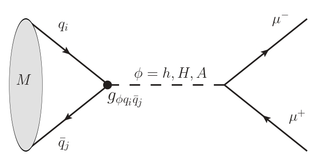
Decays of neutral mesons into muons are strongly suppressed in the theoretical framework of the SM. This suppression arises due to three key factors: (i) they occur through loop diagrams, which are inherently weaker than tree-level processes; (ii) helicity suppression reduces the probability of the interaction; and (iii) the small values of certain CKM matrix elements further diminish the decay rate. Consequently, the branching ratios for these decays are extremely low. While other channels such as electron and τ𝜏\tau decays might be theoretically possible, they are strongly suppressed and difficult to reconstruct, respectively. A representative Feynman diagram illustrating this process is shown in Fig. 1
Refer to caption
Figure 1: Generic Feynman diagram for the decays Mμ+μ𝑀superscript𝜇superscript𝜇M\to\mu^{+}\mu^{-} The black circle denotes a flavor-changing in the quark sector.

Bs,d0superscriptsubscript𝐵𝑠𝑑0B_{s,d}^{0} meson decay into μ+μsuperscript𝜇superscript𝜇\mu^{+}\mu^{-} pair, is both, interesting and stringent due to its sensitivity to constrain BSM theories. Within the theoretical framework of the SM the branching ratios read (Bs0μ+μ)=(3.66±0.14)×109superscriptsubscript𝐵𝑠0superscript𝜇superscript𝜇plus-or-minus3.660.14superscript109\mathcal{BR}(B_{s}^{0}\to\mu^{+}\mu^{-})=(3.66\pm 0.14)\times 10^{-9} and (Bd0μ+μ)=(1.03±0.05)×1010superscriptsubscript𝐵𝑑0superscript𝜇superscript𝜇plus-or-minus1.030.05superscript1010\mathcal{BR}(B_{d}^{0}\to\mu^{+}\mu^{-})=(1.03\pm 0.05)\times 10^{-10} Beneke:2019slt , while the current experimental value reported by CMS collaboration is (Bs0μ+μ)=(4.020.38+0.40(stat)0.23+0.28(syst)0.15+0.18(B))×109superscriptsubscript𝐵𝑠0superscript𝜇superscript𝜇subscriptsuperscript4.020.400.38subscriptsuperscriptstat0.280.23subscriptsuperscriptsyst0.180.15Bsuperscript109\mathcal{BR}(B_{s}^{0}\to\mu^{+}\mu^{-})=(4.02^{+0.40}_{-0.38}(\rm stat)^{+0.28}_{-0.23}(\rm syst)^{+0.18}_{-0.15}(B))\times 10^{-9}, meanwhile (Bd0μ+μ)<1.9×10¹⁰superscriptsubscript𝐵𝑑0superscript𝜇superscript𝜇1.9superscript1010\mathcal{BR}(B_{d}^{0}\to\mu^{+}\mu^{-})<1.9\times 10^{-10} at 95%percent9595\% C.L. CMS:2022mgd . In the context of the 2HDM-III, the decays Bs,d0μ+μsuperscriptsubscript𝐵𝑠𝑑0superscript𝜇superscript𝜇B_{s,d}^{0}\to\mu^{+}\mu^{-} are mediated by the SM-like Higgs boson, the heavy scalar H𝐻H and the pseudoscalar A𝐴A and it can arise at tree level. Feynman diagram for these decays is depicted in Fig. 1. For the decay Bs0μ+μsuperscriptsubscript𝐵𝑠0superscript𝜇superscript𝜇B_{s}^{0}\to\mu^{+}\mu^{-} (Bd0μ+μsuperscriptsubscript𝐵𝑑0superscript𝜇superscript𝜇B_{d}^{0}\to\mu^{+}\mu^{-}) corresponds to qi=s,q¯j=b¯formulae-sequencesubscript𝑞𝑖𝑠subscript¯𝑞𝑗¯𝑏q_{i}=s,\,\bar{q}_{j}=\bar{b} (qi=d,q¯j=b¯formulae-sequencesubscript𝑞𝑖𝑑subscript¯𝑞𝑗¯𝑏q_{i}=d,\,\bar{q}_{j}=\bar{b})

The effective Hamiltonian governing the transition Bs0μ+μsuperscriptsubscript𝐵𝑠0superscript𝜇superscript𝜇B_{s}^{0}\to\mu^{+}\mu^{-} is

effBs0μ+μ=GF2mW2π2(CAbs𝒪Abs+CSbs𝒪Sbs+CPbs𝒪Pbs+CAbs𝒪Abs+CSbs𝒪Sbs+CPbs𝒪Pbs)+h.c.,formulae-sequencesuperscriptsubscripteffsuperscriptsubscript𝐵𝑠0superscript𝜇superscript𝜇superscriptsubscript𝐺𝐹2superscriptsubscript𝑚𝑊2superscript𝜋2superscriptsubscript𝐶𝐴𝑏𝑠superscriptsubscript𝒪𝐴𝑏𝑠superscriptsubscript𝐶𝑆𝑏𝑠superscriptsubscript𝒪𝑆𝑏𝑠superscriptsubscript𝐶𝑃𝑏𝑠superscriptsubscript𝒪𝑃𝑏𝑠superscriptsubscript𝐶𝐴𝑏𝑠superscriptsubscript𝒪𝐴𝑏𝑠superscriptsubscript𝐶𝑆𝑏𝑠superscriptsubscript𝒪𝑆𝑏𝑠superscriptsubscript𝐶𝑃𝑏𝑠superscriptsubscript𝒪𝑃𝑏𝑠𝑐\mathcal{H}_{\rm eff}^{B_{s}^{0}\to\mu^{+}\mu^{-}}=-\frac{G_{F}^{2}m_{W}^{2}}{\pi^{2}}\Big{(}C_{A}^{bs}\mathcal{O}_{A}^{bs}+C_{S}^{bs}\mathcal{O}_{S}^{bs}+C_{P}^{bs}\mathcal{O}_{P}^{bs}+C_{A}^{\prime bs}\mathcal{O}_{A}^{\prime bs}+C_{S}^{\prime bs}\mathcal{O}_{S}^{\prime bs}+C_{P}^{\prime bs}\mathcal{O}_{P}^{\prime bs}\Big{)}+h.c., (25)

where the Wilson operators are given as follows

𝒪Abssuperscriptsubscript𝒪𝐴𝑏𝑠\displaystyle\mathcal{O}_{A}^{bs} =\displaystyle= (b¯γμPLs)(μ+γμγ5μ),¯𝑏subscript𝛾𝜇subscript𝑃𝐿𝑠superscript𝜇subscript𝛾𝜇subscript𝛾5superscript𝜇\displaystyle\left(\bar{b}\gamma_{\mu}P_{L}s\right)\left(\mu^{+}\gamma_{\mu}\gamma_{5}\mu^{-}\right),
𝒪Sbssuperscriptsubscript𝒪𝑆𝑏𝑠\displaystyle\mathcal{O}_{S}^{bs} =\displaystyle= (b¯PLs)(μ+μ),¯𝑏subscript𝑃𝐿𝑠superscript𝜇superscript𝜇\displaystyle\left(\bar{b}P_{L}s\right)\left(\mu^{+}\mu^{-}\right), (26)
𝒪Pbssuperscriptsubscript𝒪𝑃𝑏𝑠\displaystyle\mathcal{O}_{P}^{bs} =\displaystyle= (b¯PLs)(μ+γ5μ).¯𝑏subscript𝑃𝐿𝑠superscript𝜇subscript𝛾5superscript𝜇\displaystyle\left(\bar{b}P_{L}s\right)\left(\mu^{+}\gamma_{5}\mu^{-}\right).

The primed operators are obtained replacing PLPRsubscript𝑃𝐿subscript𝑃𝑅P_{L}\leftrightarrows P_{R}. The branching ratio for this decay is given by

(M+)=GF4mW48π514m2mM2mMfM2m2τM×[|mM2(CPijCPij)2(mi+mj)mCASM|2+|mM2(CSijCSij)2(mi+mj)m|2(14m2mM2)]𝑀superscriptsuperscriptsuperscriptsubscript𝐺𝐹4superscriptsubscript𝑚𝑊48superscript𝜋514superscriptsubscript𝑚2superscriptsubscript𝑚𝑀2subscript𝑚𝑀superscriptsubscript𝑓𝑀2superscriptsubscript𝑚2subscript𝜏𝑀missing-subexpressiondelimited-[]superscriptsuperscriptsubscript𝑚𝑀2superscriptsubscript𝐶𝑃𝑖𝑗superscriptsubscript𝐶𝑃𝑖𝑗2subscript𝑚𝑖subscript𝑚𝑗subscript𝑚superscriptsubscript𝐶𝐴SM2superscriptsuperscriptsubscript𝑚𝑀2superscriptsubscript𝐶𝑆𝑖𝑗superscriptsubscript𝐶𝑆𝑖𝑗2subscript𝑚𝑖subscript𝑚𝑗subscript𝑚214superscriptsubscript𝑚2superscriptsubscript𝑚𝑀2\displaystyle\begin{array}[]{ccl}\mathcal{BR}\left(M\rightarrow\ell^{+}\ell^{-}\right)&=&\frac{G_{F}^{4}m_{W}^{4}}{8\pi^{5}}\sqrt{1-4\frac{m_{\ell}^{2}}{m_{M}^{2}}}m_{M}f_{M}^{2}m_{\ell}^{2}\tau_{M}\\ &\times&\left[\left|\frac{m_{M}^{2}\left(C_{P}^{ij}-C_{P}^{\prime ij}\right)}{2\left(m_{i}+m_{j}\right)m_{\ell}}-C_{A}^{\rm SM}\right|^{2}+\left|\frac{m_{M}^{2}\left(C_{S}^{ij}-C_{S}^{\prime ij}\right)}{2\left(m_{i}+m_{j}\right)m_{\ell}}\right|^{2}\left(1-4\frac{m_{\ell}^{2}}{m_{M}^{2}}\right)\right]\end{array} (29)
CSijsuperscriptsubscript𝐶𝑆𝑖𝑗\displaystyle C_{S}^{ij} =\displaystyle= π22GF2mW2ϕ=h,H2gϕ+gϕijMϕ2superscript𝜋22superscriptsubscript𝐺𝐹2superscriptsubscript𝑚𝑊2italic-ϕ𝐻2subscript𝑔italic-ϕsuperscriptsuperscriptsubscript𝑔italic-ϕ𝑖𝑗superscriptsubscript𝑀italic-ϕ2\displaystyle\frac{\pi^{2}}{2G_{F}^{2}m_{W}^{2}}\underset{\phi=h,H}{\sum}\frac{2g_{\phi\ell^{+}\ell^{-}}g_{\phi ij}}{M_{\phi}^{2}}
CPijsuperscriptsubscript𝐶𝑃𝑖𝑗\displaystyle C_{P}^{ij} =\displaystyle= π22GF2mW22gϕ+gϕijMA2superscript𝜋22superscriptsubscript𝐺𝐹2superscriptsubscript𝑚𝑊22subscript𝑔italic-ϕsuperscriptsuperscriptsubscript𝑔italic-ϕ𝑖𝑗superscriptsubscript𝑀𝐴2\displaystyle\frac{\pi^{2}}{2G_{F}^{2}m_{W}^{2}}\frac{2g_{\phi\ell^{+}\ell^{-}}g_{\phi ij}}{M_{A}^{2}} (30)
CSijsuperscriptsubscript𝐶𝑆𝑖𝑗\displaystyle C_{S}^{\prime ij} =\displaystyle= CSij(gϕijgϕji)superscriptsubscript𝐶𝑆𝑖𝑗subscript𝑔italic-ϕ𝑖𝑗subscript𝑔italic-ϕ𝑗𝑖\displaystyle C_{S}^{ij}\left(g_{\phi ij}\leftrightarrows g_{\phi ji}\right)
CPijsuperscriptsubscript𝐶𝑃𝑖𝑗\displaystyle C_{P}^{\prime ij} =\displaystyle= CSij(gϕijgϕji),superscriptsubscript𝐶𝑆𝑖𝑗subscript𝑔italic-ϕ𝑖𝑗subscript𝑔italic-ϕ𝑗𝑖\displaystyle C_{S}^{ij}\left(g_{\phi ij}\leftrightarrows g_{\phi ji}\right),

where +()=μ+()superscriptsuperscript𝜇\ell^{+(-)}=\mu^{+(-)}, i=s,j=b¯formulae-sequence𝑖𝑠𝑗¯𝑏i=s,\,j=\bar{b}, mM=mBs0=5.36692subscript𝑚𝑀subscript𝑚superscriptsubscript𝐵𝑠05.36692m_{M}=m_{B_{s}^{0}}=5.36692 GeV is the Bs0superscriptsubscript𝐵𝑠0B_{s}^{0} meson mass, fM=fBs0=0.2303subscript𝑓𝑀subscript𝑓superscriptsubscript𝐵𝑠00.2303f_{M}=f_{B_{s}^{0}}=0.2303 is the Bs0superscriptsubscript𝐵𝑠0B_{s}^{0} meson decay constant, τM=τBs0=2.311×10¹²subscript𝜏𝑀subscript𝜏superscriptsubscript𝐵𝑠02.311superscript1012\tau_{M}=\tau_{B_{s}^{0}}=2.311\times 10^{12} GeV is the lifetime of the Bs0superscriptsubscript𝐵𝑠0B_{s}^{0} meson, GFsubscript𝐺𝐹G_{F} the Fermi constant and the SM contribution at one loop CASMsuperscriptsubscript𝐶𝐴SMC_{A}^{\rm SM} is given by

CASM=VtbVtsY(mt2mW2)VcbVcsY(mc2mW2),superscriptsubscript𝐶𝐴SMsuperscriptsubscript𝑉𝑡𝑏subscript𝑉𝑡𝑠𝑌superscriptsubscript𝑚𝑡2superscriptsubscript𝑚𝑊2superscriptsubscript𝑉𝑐𝑏subscript𝑉𝑐𝑠𝑌superscriptsubscript𝑚𝑐2superscriptsubscript𝑚𝑊2C_{A}^{\rm SM}=-V_{tb}^{*}V_{ts}Y\Bigg{(}\frac{m_{t}^{2}}{m_{W}^{2}}\Bigg{)}-V_{cb}^{*}V_{cs}Y\Bigg{(}\frac{m_{c}^{2}}{m_{W}^{2}}\Bigg{)}, (31)

where the function Y𝑌Y is defined as Y=ηYY0𝑌subscript𝜂𝑌subscript𝑌0Y=\eta_{Y}Y_{0} such that the NLO QCD effects are included in ηY=1.0113subscript𝜂𝑌1.0113\eta_{Y}=1.0113 Buras:2012ru and the loop Inami-Lim function Inami:1980fz reads

Y0(x)=x8[4x1x+3x(1x)2ln(x)].subscript𝑌0𝑥𝑥8delimited-[]4𝑥1𝑥3𝑥superscript1𝑥2𝑥Y_{0}(x)=\frac{x}{8}\Big{[}\frac{4-x}{1-x}+\frac{3x}{(1-x)^{2}}\ln(x)\Big{]}. (32)

To obtain the corresponding (Bd0μ+μ)superscriptsubscript𝐵𝑑0superscript𝜇superscript𝜇\mathcal{BR}(B_{d}^{0}\to\mu^{+}\mu^{-}) we carry out in Eq. (29) the replacements mBs0mBd0=5.27966subscript𝑚superscriptsubscript𝐵𝑠0subscript𝑚superscriptsubscript𝐵𝑑05.27966m_{B_{s}^{0}}\to m_{B_{d}^{0}}=5.27966 GeV, fBs0fBd0=0.190subscript𝑓superscriptsubscript𝐵𝑠0subscript𝑓superscriptsubscript𝐵𝑑00.190f_{B_{s}^{0}}\to f_{B_{d}^{0}}=0.190, τBs0τBd0=2.312×10¹²subscript𝜏superscriptsubscript𝐵𝑠0subscript𝜏superscriptsubscript𝐵𝑑02.312superscript1012\tau_{B_{s}^{0}}\to\tau_{B_{d}^{0}}=2.312\times 10^{12} GeV; In Eqs. (III.1.1) gϕb¯sgϕb¯dsubscript𝑔italic-ϕ¯𝑏𝑠subscript𝑔italic-ϕ¯𝑏𝑑g_{\phi\bar{b}s}\to g_{\phi\bar{b}d} and in Eqs. (III.1.1) sd𝑠𝑑s\to d.

Lepton flavor violating processes

III.1.2 Muon anomalous magnetic moment aμsubscript𝑎𝜇a_{\mu}

Given (still) the current discrepancy between the experimental measurement and the SM theoretical prediction of aμsubscript𝑎𝜇a_{\mu}, we use it to constrain the free model parameters that have an impact in that observable. The Feynman diagrams that contribute to aμsubscript𝑎𝜇a_{\mu} are shown in Fig. 2.

Refer to caption
Figure 2: Feynman diagrams that contribute to aμsubscript𝑎𝜇a_{\mu}. Here ϕitalic-ϕ\phi represents a CP-even scalar, CP-odd scalar and the SM-like Higgs boson. H±superscript𝐻plus-or-minusH^{\pm} stand for charged scalar bosons. Here i=μsubscript𝑖𝜇\ell_{i}=\mu.

The contributions at one-loop level reads

δaμϕ=GFmμ24π22igμi2RϕFϕ(Rϕ),𝛿superscriptsubscript𝑎𝜇italic-ϕsubscript𝐺𝐹superscriptsubscript𝑚𝜇24superscript𝜋22subscriptsubscript𝑖superscriptsubscript𝑔𝜇subscript𝑖2subscript𝑅italic-ϕsubscript𝐹italic-ϕsubscript𝑅italic-ϕ\delta a_{\mu}^{\phi}=\frac{G_{F}m_{\mu}^{2}}{4\pi^{2}\sqrt{2}}\sum_{\ell_{i}}g_{\mu\ell_{i}}^{2}R_{\phi}F_{\phi}(R_{\phi}), (33)

with

Fh,Hsubscript𝐹𝐻\displaystyle F_{h,\,H} =\displaystyle= 01𝑑xx2(2x)Rh,Hx2x+1,superscriptsubscript01differential-d𝑥superscript𝑥22𝑥subscript𝑅𝐻superscript𝑥2𝑥1\displaystyle\int_{0}^{1}dx\frac{x^{2}(2-x)}{R_{h,\,H}x^{2}-x+1}, (34)
FAsubscript𝐹𝐴\displaystyle F_{A} =\displaystyle= 01𝑑xx3RAx2x+1,superscriptsubscript01differential-d𝑥superscript𝑥3subscript𝑅𝐴superscript𝑥2𝑥1\displaystyle\int_{0}^{1}dx\frac{-x^{3}}{R_{A}x^{2}-x+1}, (35)
FH±superscriptsubscript𝐹𝐻plus-or-minus\displaystyle F_{H}^{\pm} =\displaystyle= 01𝑑xx2(1x)RH±x2+(1RH±)x.superscriptsubscript01differential-d𝑥superscript𝑥21𝑥subscript𝑅superscript𝐻plus-or-minussuperscript𝑥21subscript𝑅superscript𝐻plus-or-minus𝑥\displaystyle\int_{0}^{1}dx\frac{-x^{2}(1-x)}{R_{H^{\pm}}x^{2}+(1-R_{H^{\pm}})x}. (36)

where Rϕ=mμ2/Mϕ2subscript𝑅italic-ϕsubscriptsuperscript𝑚2𝜇subscriptsuperscript𝑀2italic-ϕR_{\phi}=m^{2}_{\mu}/M^{2}_{\phi} (ϕ=h,H,A,H±italic-ϕ𝐻𝐴superscript𝐻plus-or-minus\phi=h,\,H,\,A,\,H^{\pm}). While the dominant contribution at two-loops is induced by A𝐴A circulating inside the loop kind box, and is given by

δaμ2loops=α28π2sW2mμ2gAμμmW2fNcfQf2RAF¯AgAfif¯j,𝛿superscriptsubscript𝑎𝜇2𝑙𝑜𝑜𝑝𝑠superscript𝛼28superscript𝜋2superscriptsubscript𝑠𝑊2superscriptsubscript𝑚𝜇2subscript𝑔𝐴𝜇𝜇superscriptsubscript𝑚𝑊2subscript𝑓superscriptsubscript𝑁𝑐𝑓superscriptsubscript𝑄𝑓2subscript𝑅𝐴subscript¯𝐹𝐴subscript𝑔𝐴subscript𝑓𝑖subscript¯𝑓𝑗\delta a_{\mu}^{2-loops}=\frac{\alpha^{2}}{8\pi^{2}s_{W}^{2}}\frac{m_{\mu}^{2}g_{A\mu\mu}}{m_{W}^{2}}\sum_{f}N_{c}^{f}Q_{f}^{2}R_{A}\bar{F}_{A}g_{Af_{i}\bar{f}_{j}}, (37)

where

F¯A=01𝑑ylog(RAy(1y))RAy(1RA)subscript¯𝐹𝐴superscriptsubscript01differential-d𝑦subscript𝑅𝐴𝑦1𝑦subscript𝑅𝐴𝑦1subscript𝑅𝐴\bar{F}_{A}=\int_{0}^{1}dy\frac{\log\Big{(}\frac{R_{A}}{y(1-y)}\Big{)}}{R_{A}-y(1-R_{A})} (38)

III.1.3 ijγsubscript𝑖subscript𝑗𝛾\ell_{i}\to\ell_{j}\gamma decays

The effective Lagrangian for the ijγsubscript𝑖subscript𝑗𝛾\ell_{i}\to\ell_{j}\gamma is given by

eff=CLQLγCRQRγ+h.c.,formulae-sequencesubscripteffsubscript𝐶𝐿subscript𝑄𝐿𝛾subscript𝐶𝑅subscript𝑄𝑅𝛾𝑐\mathcal{L}_{\text{eff}}=C_{L}Q_{L\gamma}C_{R}Q_{R\gamma}+h.c., (39)

where the dim-5 electromagnetic penguin operators read

QLγ,Rγ=e8π2(¯jσαβPL,Ri)Fαβ,subscript𝑄𝐿𝛾𝑅𝛾𝑒8superscript𝜋2subscript¯𝑗superscript𝜎𝛼𝛽subscript𝑃𝐿𝑅subscript𝑖subscript𝐹𝛼𝛽Q_{L\gamma,\,R\gamma}=\frac{e}{8\pi^{2}}(\bar{\ell}_{j}\sigma^{\alpha\beta}P_{L,\,R}\ell_{i})F_{\alpha\beta}, (40)

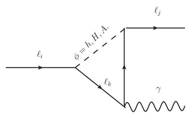
here Fαβsubscript𝐹𝛼𝛽F_{\alpha\beta} is the electromagnetic field strength tensor. The Feynman diagram of the process ijγsubscript𝑖subscript𝑗𝛾\ell_{i}\to\ell_{j}\gamma is depicted in Fig. 3.

Refer to caption
Figure 3: Feynman diagram of the process ijγsubscript𝑖subscript𝑗𝛾\ell_{i}\to\ell_{j}\gamma at one-loop level induced by ϕ=h,H,Aitalic-ϕ𝐻𝐴\phi=h,\,H,\,A.

The Wilson coefficients CL,Rsubscript𝐶𝐿𝑅C_{L,\,R} receive contributions at one-loop level and an important contribution from the Barr-Zee two-loops level. For the particular case where i=τsubscript𝑖𝜏\ell_{i}=\tau and j=μsubscript𝑗𝜇\ell_{j}=\mu, the approximations gϕμμgϕττmuch-less-thansubscript𝑔italic-ϕ𝜇𝜇subscript𝑔italic-ϕ𝜏𝜏g_{\phi\mu\mu}\ll g_{\phi\tau\tau} and mμmτmϕmuch-less-thansubscript𝑚𝜇subscript𝑚𝜏much-less-thansubscript𝑚italic-ϕm_{\mu}\ll m_{\tau}\ll m_{\phi} are assumed. According to this assertion, the one-loop Wilson coefficients CL,Rsubscript𝐶𝐿𝑅C_{L,\,R} simplify as follows Harnik:2012pb ; Blankenburg:2012ex

CL1loopϕgϕττgϕτμ12mϕ2(4+3logmϕ2mτ2),CR2loopϕgϕττgϕτμ12mϕ2(4+3logmϕ2mτ2),formulae-sequencesimilar-to-or-equalssuperscriptsubscript𝐶𝐿1𝑙𝑜𝑜𝑝subscriptitalic-ϕsubscript𝑔italic-ϕ𝜏𝜏subscript𝑔italic-ϕ𝜏𝜇12superscriptsubscript𝑚italic-ϕ243superscriptsubscript𝑚italic-ϕ2superscriptsubscript𝑚𝜏2similar-to-or-equalssuperscriptsubscript𝐶𝑅2𝑙𝑜𝑜𝑝subscriptitalic-ϕsubscript𝑔italic-ϕ𝜏𝜏subscript𝑔italic-ϕ𝜏𝜇12superscriptsubscript𝑚italic-ϕ243superscriptsubscript𝑚italic-ϕ2superscriptsubscript𝑚𝜏2C_{L}^{1loop}\simeq\sum_{\phi}\frac{g_{\phi\tau\tau}g_{\phi\tau\mu}}{12m_{\phi}^{2}}\Bigg{(}-4+3\log\frac{m_{\phi}^{2}}{m_{\tau}^{2}}\Bigg{)},\;\;\;C_{R}^{2loop}\simeq\sum_{\phi}\frac{g_{\phi\tau\tau}g_{\phi\tau\mu}}{12m_{\phi}^{2}}\Bigg{(}-4+3\log\frac{m_{\phi}^{2}}{m_{\tau}^{2}}\Bigg{)}, (41)

The numerical expressions for 2-loop contributions are given by

CL2loops=ϕ=h,H,Agϕτμ(0.082gϕtt+0.11)/(mϕGeV)2.superscriptsubscript𝐶𝐿2𝑙𝑜𝑜𝑝𝑠subscriptitalic-ϕ𝐻𝐴subscript𝑔italic-ϕ𝜏𝜇0.082subscript𝑔italic-ϕ𝑡𝑡0.11superscriptsubscript𝑚italic-ϕGeV2C_{L}^{2-loops}=\sum_{\phi=h,\,H,\,A}g_{\phi\tau\mu}(-0.082g_{\phi tt}+0.11)/(m_{\phi}\text{GeV})^{2}. (42)

The rate for τμγ𝜏𝜇𝛾\tau\to\mu\gamma is

Γ(τμγ)=αmτ264π4(|CL|2+|CR|2).Γ𝜏𝜇𝛾𝛼superscriptsubscript𝑚𝜏264superscript𝜋4superscriptsubscript𝐶𝐿2superscriptsubscript𝐶𝑅2\Gamma(\tau\to\mu\gamma)=\frac{\alpha m_{\tau}^{2}}{64\pi^{4}}(|C_{L}|^{2}+|C_{R}|^{2}). (43)

To obtain the corresponding width decay of the processes μeγ𝜇𝑒𝛾\mu\to e\gamma and τeγ𝜏𝑒𝛾\tau\to e\gamma, the replacements τμ,μeformulae-sequence𝜏𝜇𝜇𝑒\tau\to\mu,\,\mu\to e for the former decay and μe𝜇𝑒\mu\to e for the second process from (39) to (43) are required.

III.1.4 ijk¯ksubscript𝑖subscript𝑗subscript𝑘subscript¯𝑘\ell_{i}\to\ell_{j}\ell_{k}\bar{\ell}_{k} decays

Within the 2HDM-III framework, these kinds of decays can occur at tree-level via the exchange of h,H,A𝐻𝐴h,\,H,\,A, as shown in Fig. 4. Nevertheless, the process is suppressed by the flavor violating Yukawa couplings Yijsubscript𝑌subscript𝑖subscript𝑗Y_{\ell_{i}\ell_{j}} and by the flavor-conserving coupling Ykksubscript𝑌subscript𝑘subscript𝑘Y_{\ell_{k}\ell_{k}}.

Refer to caption
Figure 4: Feynman diagrams that contribute to the ijk¯ksubscript𝑖subscript𝑗subscript𝑘subscript¯𝑘\ell_{i}\to\ell_{j}\ell_{k}\bar{\ell}_{k}, (a) tree-level and (b) one-loop level, where the black circle represents the loop as Feynman diagram of Fig. 3

III.1.5 hijsubscript𝑖subscript𝑗h\to\ell_{i}\ell_{j} decays

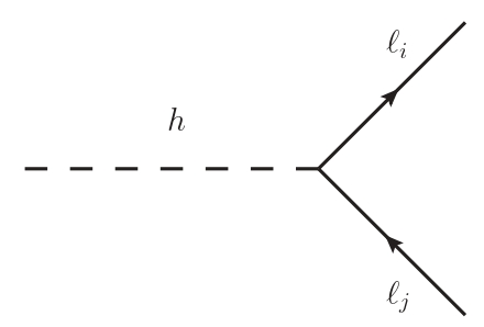
The LFV processes hijsubscript𝑖subscript𝑗h\to\ell_{i}\ell_{j} (i,j=i,ji,j+subscript𝑖𝑗superscriptsubscript𝑖𝑗superscriptsubscript𝑖𝑗\ell_{i,\,j}=\ell_{i,\,j}^{-}\ell_{i,\,j}^{+}) where ij=eμ,eτ,τμsubscript𝑖subscript𝑗𝑒𝜇𝑒𝜏𝜏𝜇\ell_{i}\ell_{j}=e\mu,\,e\tau,\,\tau\mu can arise at tree level in many models that extend to the SM, as shown in Fig. 5.
Refer to caption
Figure 5: Feynman diagram of the process hijsubscript𝑖subscript𝑗h\to\ell_{i}\ell_{j} at tree level.

The relevant interactions can be extracted from the Yukawa Lagrangian

YYij¯LiRjh+h.c.formulae-sequencesubscript𝑌𝑖𝑗superscriptsubscript¯𝐿𝑖superscriptsubscript𝑅𝑗subscript𝑌𝑐\mathcal{L}_{Y}\supset-Y_{ij}\bar{\ell}_{L}^{i}\ell_{R}^{j}h+h.c. (44)

The corresponding full decay width of the hf¯ifjsubscript¯𝑓𝑖subscript𝑓𝑗h\to\bar{f}_{i}f_{j} decays is given by:

Γ(hf¯ifj)=Ncghf¯ifj2mh128π[4(τfi+τfj)2]3/24(τfiτfj)2,Γsubscript¯𝑓𝑖subscript𝑓𝑗subscript𝑁𝑐subscriptsuperscript𝑔2subscript¯𝑓𝑖subscript𝑓𝑗subscript𝑚128𝜋superscriptdelimited-[]4superscriptsubscript𝜏subscript𝑓𝑖subscript𝜏subscript𝑓𝑗2324superscriptsubscript𝜏subscript𝑓𝑖subscript𝜏subscript𝑓𝑗2\Gamma(h\to\bar{f}_{i}f_{j})=\frac{N_{c}g^{2}_{h\bar{f}_{i}f_{j}}m_{h}}{128\pi}\Bigg{[}4-(\sqrt{\tau_{f_{i}}}+\sqrt{\tau_{f_{j}}})^{2}\Bigg{]}^{3/2}\sqrt{4-(\sqrt{\tau_{f_{i}}}-\sqrt{\tau_{f_{j}}})^{2}}, (45)

where ghf¯ifjsubscript𝑔subscript¯𝑓𝑖subscript𝑓𝑗g_{h\bar{f}_{i}f_{j}} is the hf¯ifjsubscript¯𝑓𝑖subscript𝑓𝑗h\bar{f}_{i}f_{j} coupling coming from an extension of the SM, Nc=3(1)𝑁𝑐31Nc=3\,(1) is the color number for quarks (leptons), mhsubscript𝑚m_{h} is the Higgs boson mass and τi=4mi2/mh2subscript𝜏𝑖4superscriptsubscript𝑚𝑖2superscriptsubscript𝑚2\tau_{i}=4m_{i}^{2}/m_{h}^{2}.

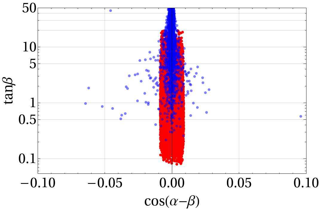
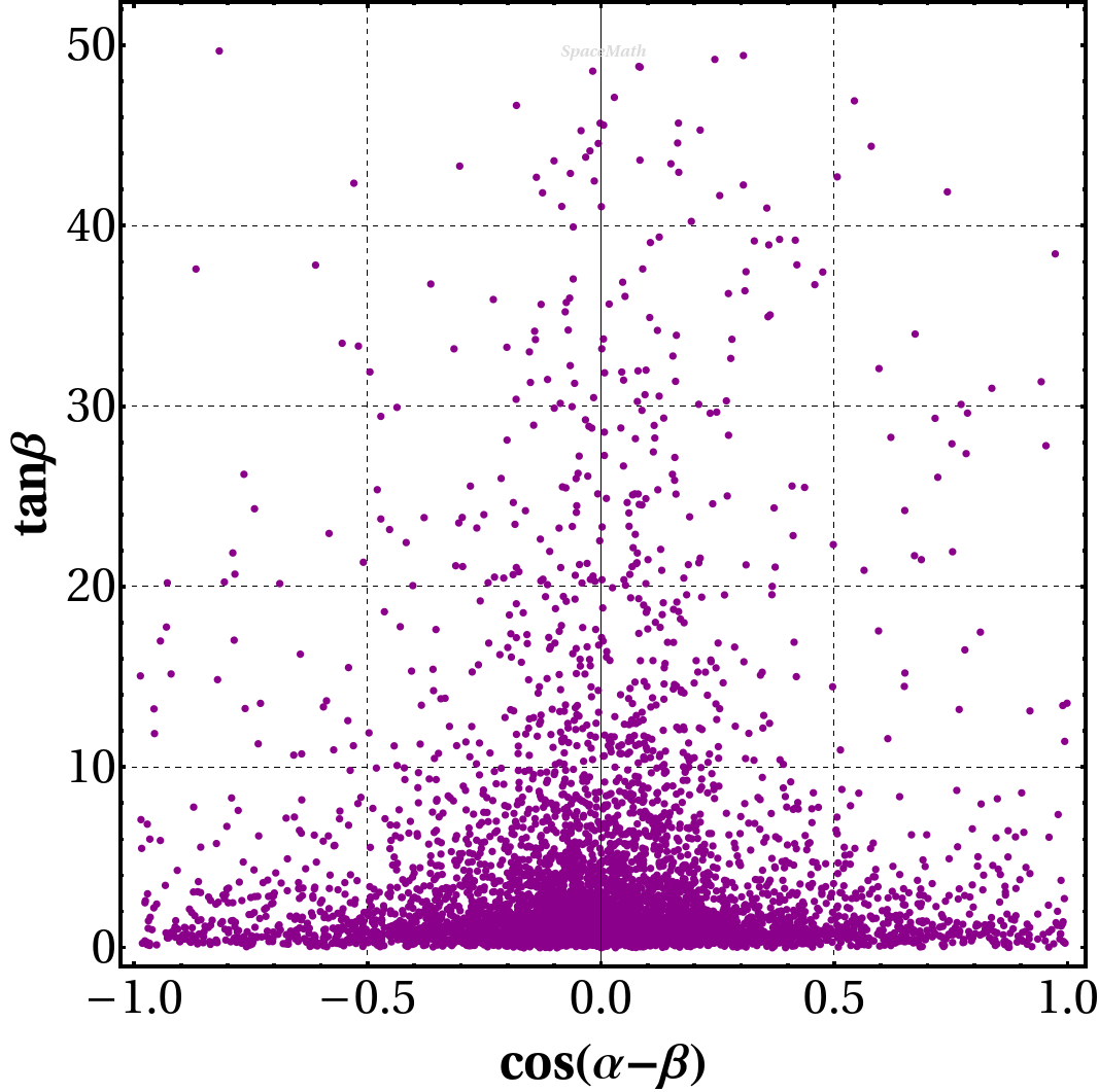
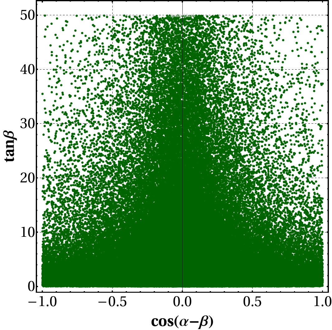
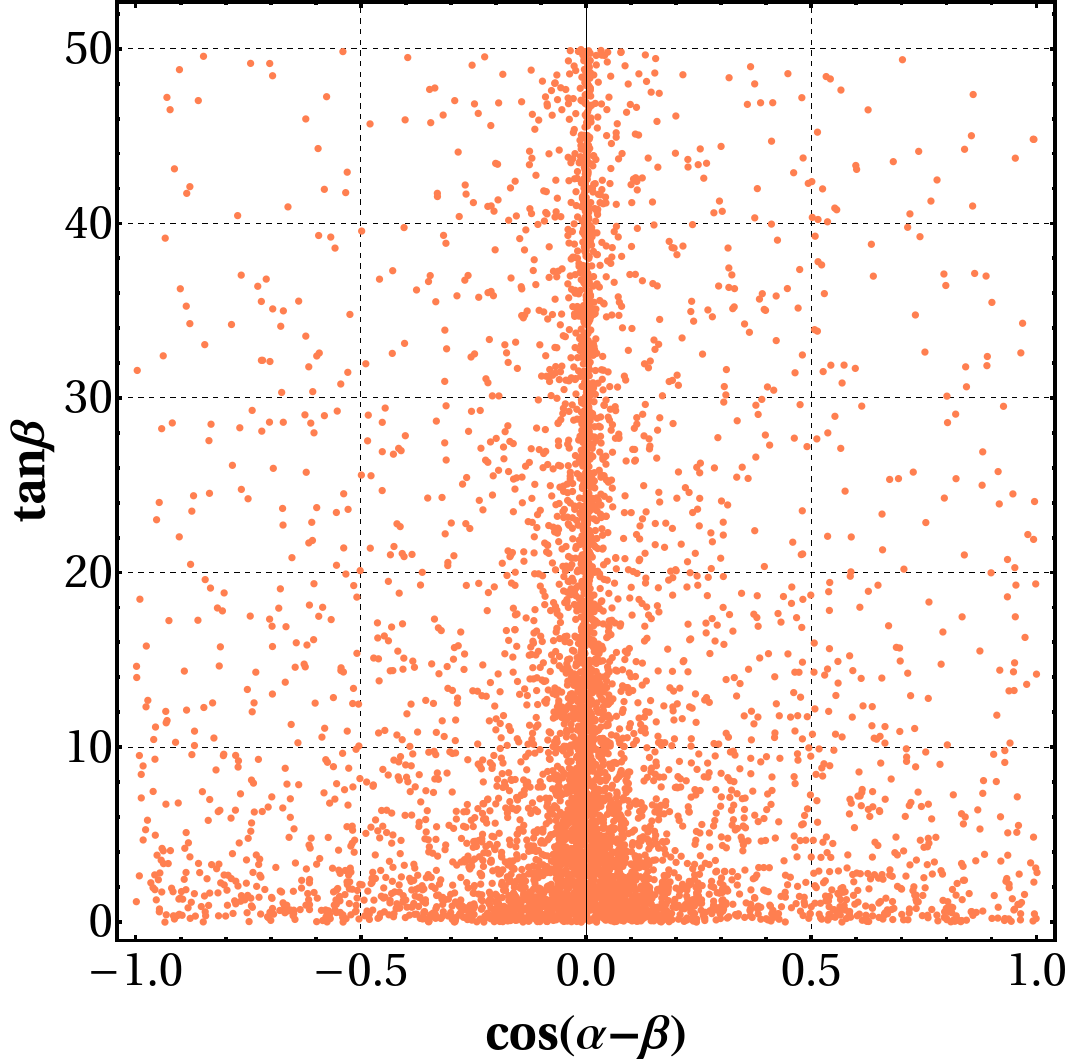
Once all the analytical expressions to calculate the BRs of the exposed observables have been given, we evaluate all the processes in Sec. III with the Mathematica package so-called SpaceMath333This software has implemented all the experimental constraints considered in our project. Arroyo-Urena:2020qup in order to find the values of the free parameters involved in our analysis. In Fig. 6, we present the cos(αβ)tanβ𝛼𝛽𝛽\cos(\alpha-\beta)-\tan\beta plane, whose points represent the allowed values in such a plane. The red points represent the measurements allowed (or upper limits) on branching ratios of the Bs,dμ+μsubscript𝐵𝑠𝑑superscript𝜇superscript𝜇B_{s,d}\to\mu^{+}\mu^{-} and the LFV processes, while the blue points stand for these measurements allowed by LHC Higgs boson data. We find a very restricted parameter space in that plane, if one considers the allowed region by all the observables, 0.01cos(αβ)0.01less-than-or-similar-to0.01𝛼𝛽less-than-or-similar-to0.01-0.01\lesssim\cos(\alpha-\beta)\lesssim 0.01 for 0.5tanβ20less-than-or-similar-to0.5𝛽less-than-or-similar-to200.5\lesssim\tan\beta\lesssim 20.

Refer to caption
Figure 6: Blue (Red) points stand for these allowed values by all the signal strength modifiers μXsubscript𝜇𝑋\mathcal{\mu}_{X} (LFV processes). All the allowed values are presented in the cos(αβ)tanβ𝛼𝛽𝛽\cos(\alpha-\beta)-\tan\beta plane.

We include in Appx. Constraints individual allowed values of the model parameters associated with each observable.

III.2 Constraint on MHsubscript𝑀𝐻M_{H}, MAsubscript𝑀𝐴M_{A} and MH±subscript𝑀superscript𝐻plus-or-minusM_{H^{\pm}}

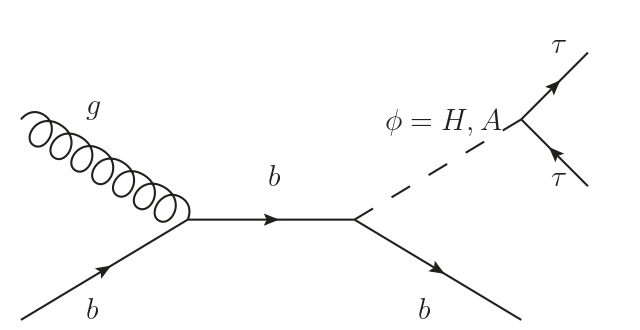
The ATLAS and CMS collaborations presented results of a search for additional neutral Higgs bosons in the ditau decay channel ATLAS-CONF ; Sirunyan:2018zut . The former of them searched through the process gbϕττ𝑔𝑏italic-ϕ𝜏𝜏gb\to\phi\to\tau\tau, with ϕ=A,Hitalic-ϕ𝐴𝐻\phi=A,\,H; Fig. 7 shows the Feynman diagram of the process. However, no evidence of any additional Higgs boson was observed, but upper limits on the production cross-section σ(gbϕ)𝜎𝑔𝑏italic-ϕ\sigma(gb\to\phi) times branching ratio (ϕττ)italic-ϕ𝜏𝜏\mathcal{BR}(\phi\to\tau\tau) were imposed.

Refer to caption
Figure 7: Feynman diagram of the production of ϕitalic-ϕ\phi in association with a bottom quark at LHC, with a subsequent decay into a ττ𝜏𝜏\tau\tau pair.

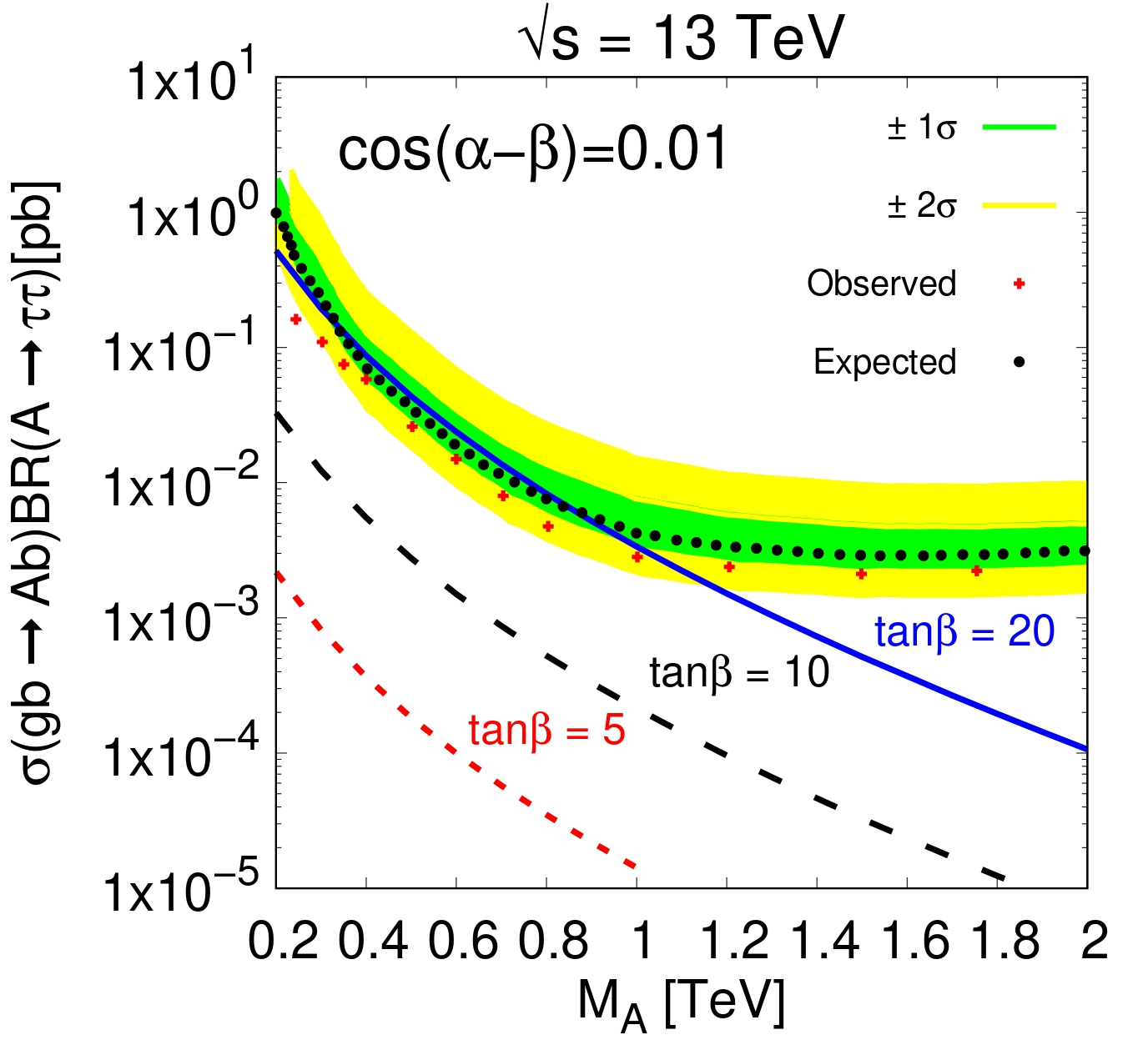
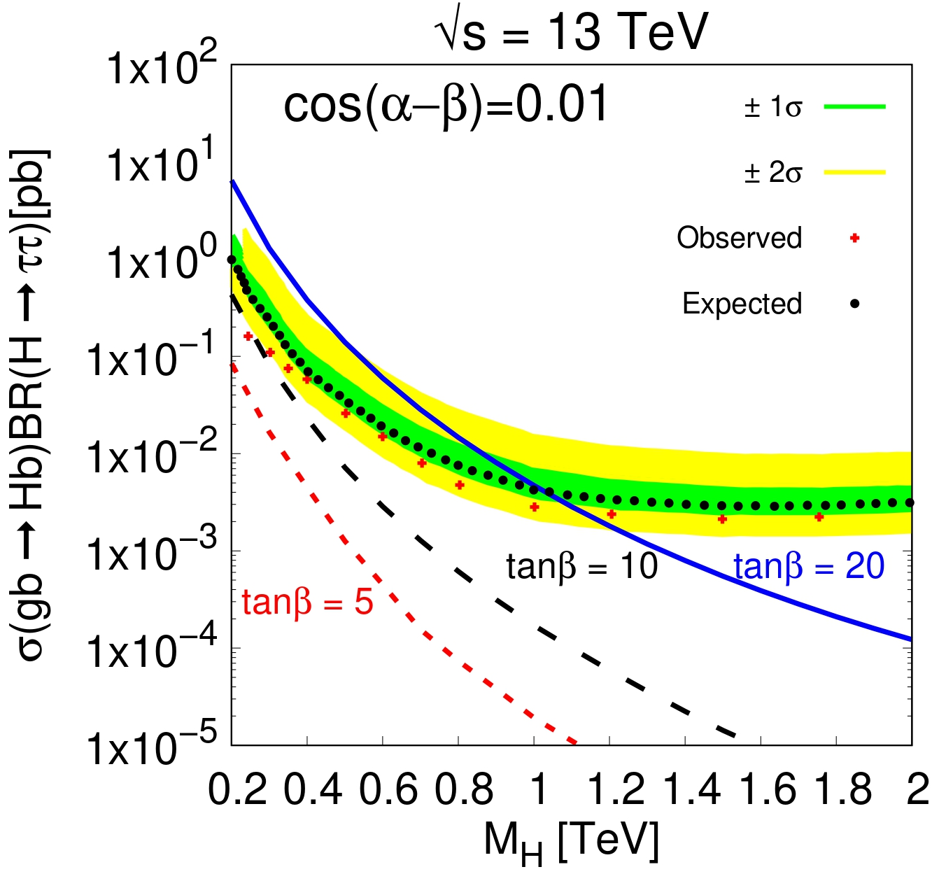
Figure 8(a) presents the σ(gbAb)×(Aττ)𝜎𝑔𝑏𝐴𝑏𝐴𝜏𝜏\sigma(gb\to Ab)\times\mathcal{BR}(A\to\tau\tau) as a function of MAsubscript𝑀𝐴M_{A} for illustrative values of tanβ=5, 10, 20𝛽51020\tan{\beta}=5,\,10,\,20 and cos(αβ)=0.01𝛼𝛽0.01\cos(\alpha-\beta)=0.01. Figure 8(b) shows the same but for ϕ=Hitalic-ϕ𝐻\phi=H. In both plots, the black points and the red crosses represent the expected and observed values at 95%percent\% CL upper limits, respectively; while the green (yellow) band indicates the interval at ±1σplus-or-minus1𝜎\pm 1\sigma (±2σplus-or-minus2𝜎\pm 2\sigma) with respect to the expected value.

Refer to caption
(a)
Refer to caption
(b)
Figure 8: The observed and expected at 95%percent\% CL upper limits on the production cross-section times ditau branching ratio for a scalar boson produced via b𝑏b-associated production as a function of (a) MAsubscript𝑀𝐴M_{A} (b) MHsubscript𝑀𝐻M_{H}. In both cases we consider tβ=subscript𝑡𝛽absentt_{\beta}= 5, 8, 20 and cαβ=0.01subscript𝑐𝛼𝛽0.01c_{\alpha\beta}=0.01.

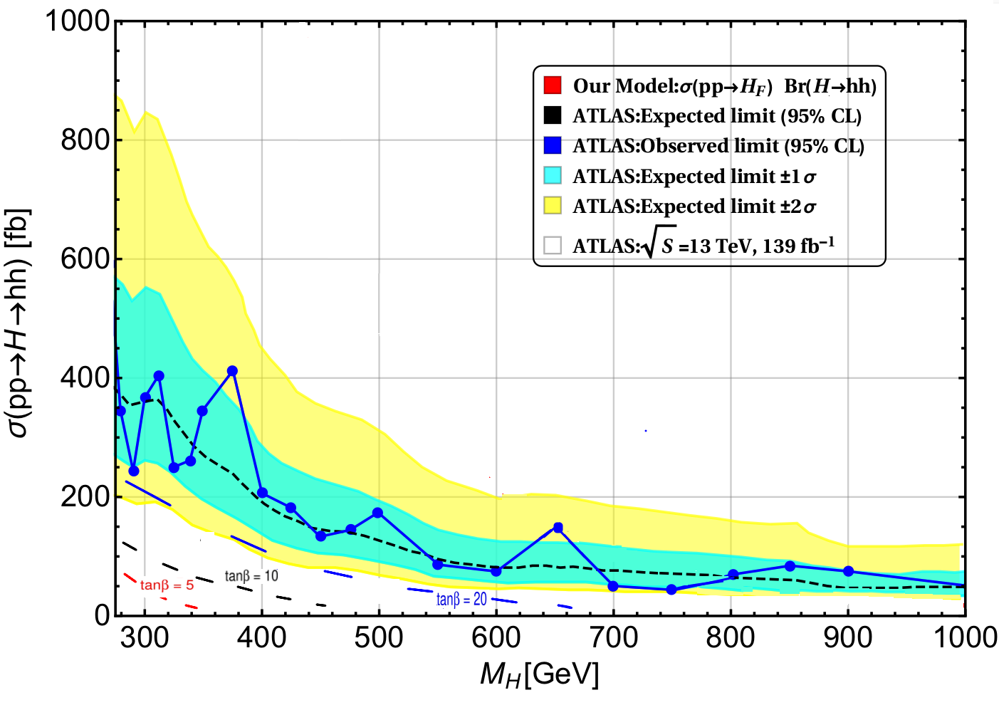
From Fig. 8(a) we note that MA1less-than-or-similar-tosubscript𝑀𝐴1M_{A}\lesssim 1 TeV (MA1.2less-than-or-similar-tosubscript𝑀𝐴1.2M_{A}\lesssim 1.2 TeV) are excluded at 1σ𝜎\sigma (2σ𝜎\sigma) for tanβ=20𝛽20\tan{\beta}=20, while for tanβ5, 10less-than-or-similar-to𝛽510\tan{\beta}\lesssim 5,\,10 the upper limit on σ(gbϕb)×(ϕττ)𝜎𝑔𝑏italic-ϕ𝑏italic-ϕ𝜏𝜏\sigma(gb\to\phi b)\times\mathcal{BR}(\phi\to\tau\tau) is easily accomplished. Meanwhile, from Fig. 8(b), we find MH1.1less-than-or-similar-tosubscript𝑀𝐻1.1M_{H}\lesssim 1.1 TeV (MHless-than-or-similar-tosubscript𝑀𝐻absentM_{H}\lesssim 1.3 GeV) are excluded at 1σ𝜎\sigma (2σ𝜎\sigma) for tanβ=20𝛽20\tan{\beta}=20. Another process used to constrain the mass of the heavy scalar MHsubscript𝑀𝐻M_{H} is when it decays into a Higgs boson pair with their subsequent decays to bb¯𝑏¯𝑏b\bar{b} and γγ𝛾𝛾\gamma\gamma, i.e., ppHhh,hbb¯,hγγformulae-sequence𝑝𝑝𝐻formulae-sequence𝑏¯𝑏𝛾𝛾pp\to H\to hh,h\to b\bar{b},h\to\gamma\gamma. Figure 9 presents the cross-section σ(ppHhh,hbb¯,hγγ)\sigma(pp\to H\to hh,h\to b\bar{b},h\to\gamma\gamma) as a function of MHsubscript𝑀𝐻M_{H} including the upper limits at 1σ𝜎\sigma (green band) and at 2σ𝜎\sigma (yellow band), the expected limit (segmented black line) and the observed limit (blue line). These results were reported by the ATLAS collaboration ATLAS:2021ifb . On the same plot, we also add the prediction of the 2HDM-III for tanβ=5, 10, 20𝛽51020\tan\beta=5,\,10,\,20 and cos(αβ)=0.01𝛼𝛽0.01\cos(\alpha-\beta)=0.01. However, we found that the aforementioned limits are easily met.
Refer to caption
Figure 9: The observed and expected at 95%percent\% CL upper limits on the production cross-section times di-Higgs branching ratio for a scalar boson produced via pp𝑝𝑝pp collisions as a function of MHsubscript𝑀𝐻M_{H}. We consider tanβ=𝛽absent\tan{\beta}= 5, 10, 20 and cos(αβ)=0.01𝛼𝛽0.01\cos(\alpha-\beta)=0.01.

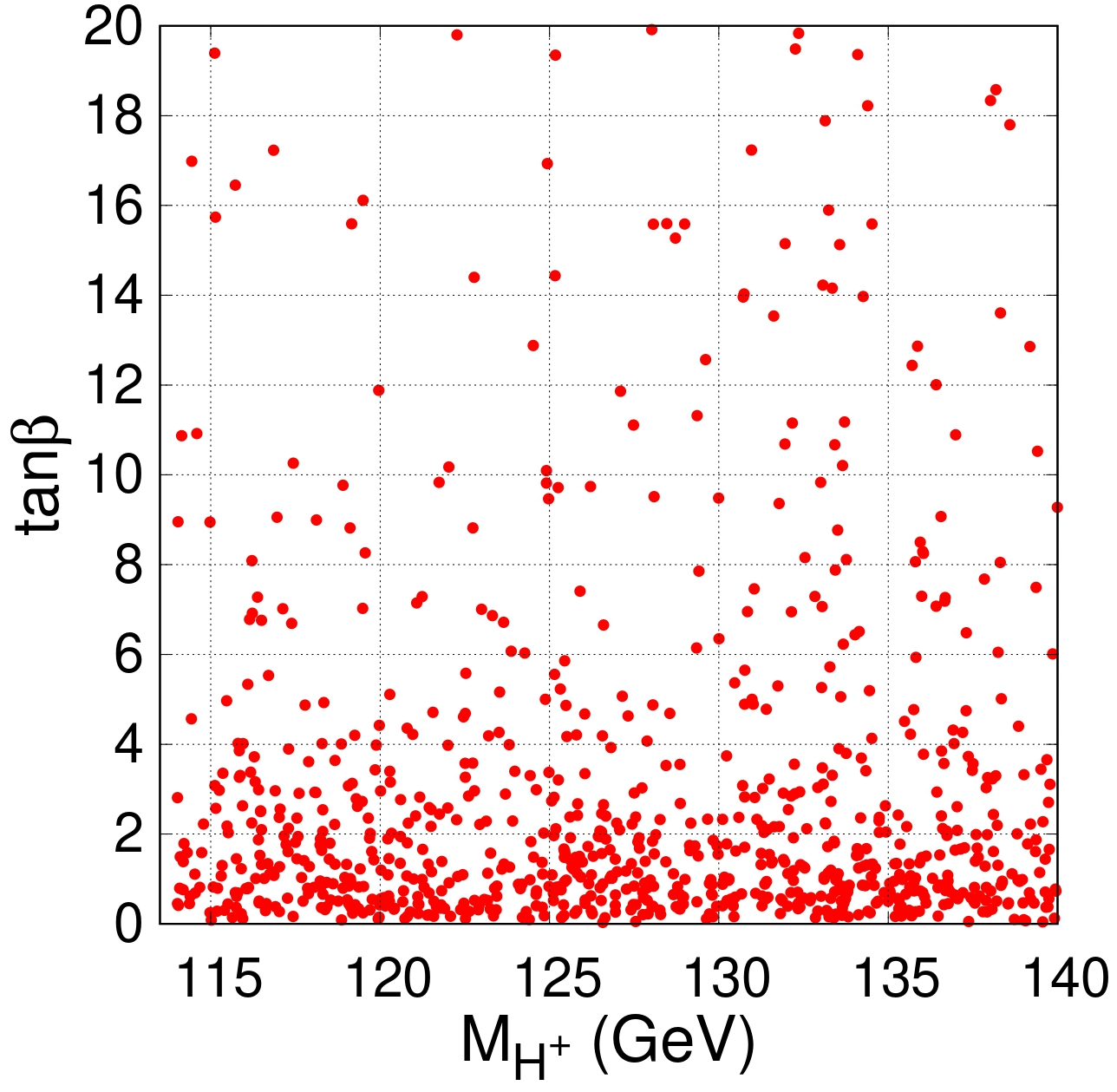
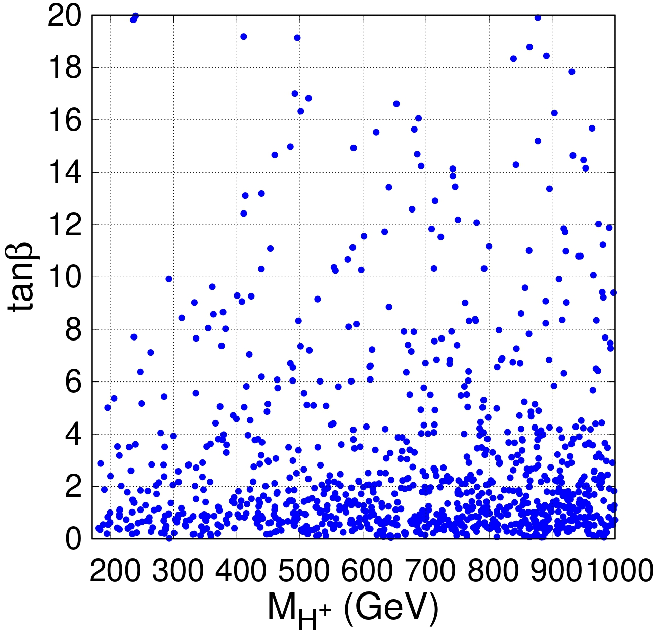
Concerning to the charged scalar boson H±superscript𝐻plus-or-minusH^{\pm}, its detection would represent a clear signature of new physics. Constraints on its mass MH±subscript𝑀superscript𝐻plus-or-minusM_{H^{\pm}} were obtained from collider searches for the H±superscript𝐻plus-or-minusH^{\pm} production and its subsequent decay into a τ±ντsuperscript𝜏plus-or-minussubscript𝜈𝜏\tau^{\pm}\nu_{\tau} pair ATLAS:2018gfm . However, we find that such processes are not a good way to constrain the charged scalar mass MH±subscript𝑀superscript𝐻plus-or-minusM_{H^{\pm}} predicted in 2HDM-III. Nevertheless, the situation is opposite if one considers the decay bsγ𝑏𝑠𝛾b\to s\gamma which imposes severe lower limits on MH±subscript𝑀superscript𝐻plus-or-minusM_{H^{\pm}} because of the charged boson contribution Ciuchini:1997xe ; Misiak:2017bgg . Figure 10(a)-(b) shows a scatter plot in the MH±subscript𝑀superscript𝐻plus-or-minusM_{H^{\pm}}-tanβ𝛽\tan\beta plane whose red and blue points stand for these allowed by the ratio Rquarksubscript𝑅quarkR_{\rm quark}, defined as follows:

Rquark=Γ(bXsγ)Γ(bXceνe).subscript𝑅quarkΓ𝑏subscript𝑋𝑠𝛾Γ𝑏subscript𝑋𝑐𝑒subscript𝜈𝑒R_{\rm quark}=\frac{\Gamma(b\to X_{s}\gamma)}{\Gamma(b\to X_{c}e\nu_{e})}. (46)
Refer to caption
Refer to caption
Figure 10: Scatter plot in the MH±tanβsubscript𝑀superscript𝐻plus-or-minus𝛽M_{H^{\pm}}-\tan\beta plane. (a) Red points stand for these allowed by Rquarksubscript𝑅quarkR_{\rm quark} for the 114MH±140114subscript𝑀superscript𝐻plus-or-minus140114\leq M_{H^{\pm}}\leq 140 GeV interval. (b) The same as in (a) but for the range of masses mt+mbMH±1000subscript𝑚𝑡subscript𝑚𝑏subscript𝑀superscript𝐻plus-or-minus1000m_{t}+m_{b}\leq M_{H^{\pm}}\leq 1000. Rquarksubscript𝑅quarkR_{\rm quark} is defined in Eq. (46).

We note a preference for low tanβ𝛽\tan\beta in both mass ranges, namely 114MH±140114subscript𝑀superscript𝐻plus-or-minus140114\leq M_{H^{\pm}}\leq 140 GeV and mt+mbMH±1000subscript𝑚𝑡subscript𝑚𝑏subscript𝑀superscript𝐻plus-or-minus1000m_{t}+m_{b}\leq M_{H^{\pm}}\leq 1000 GeV. This is due to the form of the contributions coming from 2HDM-III: gu¯dH1/tanβ(1χtt/2)similar-tosubscript𝑔¯𝑢𝑑superscript𝐻1𝛽1subscript𝜒𝑡𝑡2g_{\bar{u}dH^{-}}\sim 1/\tan\beta(1-\chi_{tt}/\sqrt{2}) and gd¯uH+tanβ(1χbb/2)similar-tosubscript𝑔¯𝑑𝑢superscript𝐻𝛽1subscript𝜒𝑏𝑏2g_{\bar{d}uH^{+}}\sim\tan\beta(1-\chi_{bb}/\sqrt{2}) of which we can observe that a large tanβ𝛽\tan\beta would give dangerous contributions to bsγ𝑏𝑠𝛾b\to s\gamma. The former scanned mass range is motivated by the current excess of events reported by the ATLAS collaboration ATLAS:2023bzb .

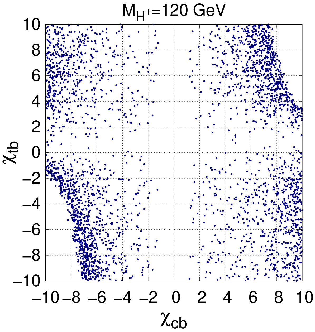
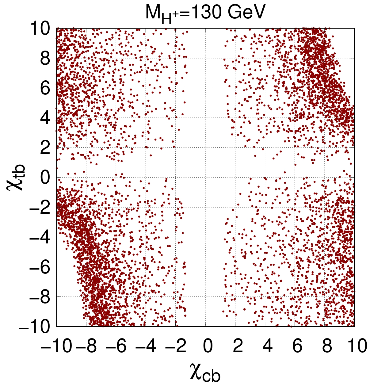
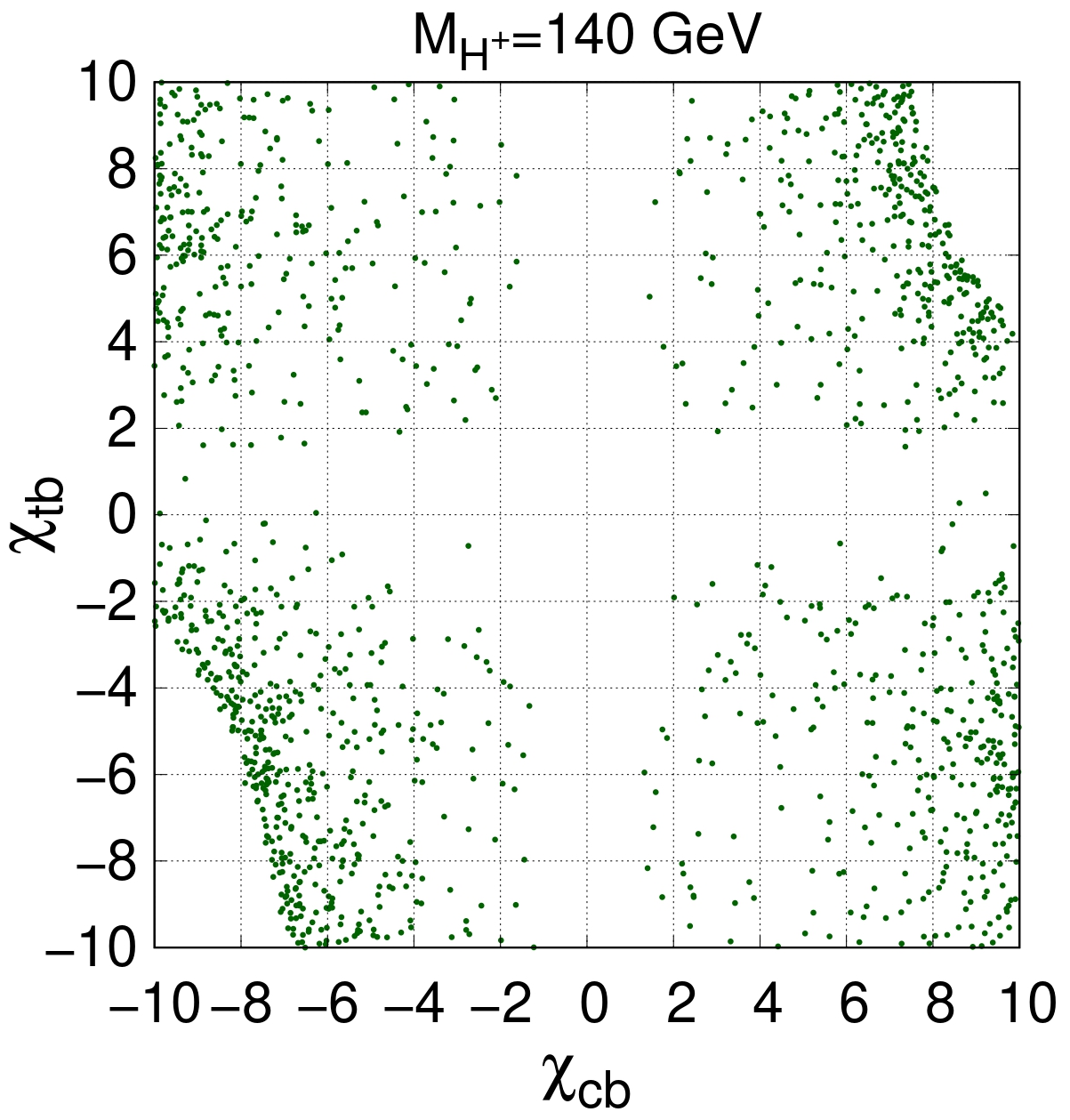
Since our analysis focuses on the case of low-charged scalar masses (MH±<mt+mbsubscript𝑀superscript𝐻plus-or-minussubscript𝑚𝑡subscript𝑚𝑏M_{H^{\pm}}<m_{t}+m_{b}), it is worth mentioning that the model under consideration may explain the recent slight excess in data with a significance of around 3σ3𝜎3\sigma for MH±=130subscript𝑀superscript𝐻plus-or-minus130M_{H^{\pm}}=130 GeV reported by the ATLAS collaboration ATLAS:2023bzb . This search used a data set of collisions pp𝑝𝑝pp collected at a center-of-mass energy s=13𝑠13\sqrt{s}=13 TeV amounting to an integrated luminosity of 139 fb-1. The analysis focuses on a data sample enriched in top-quark pair production, where one top quark decays into a leptonically decaying W𝑊W boson and a bottom quark, and the other top quark may decay into a H±superscript𝐻plus-or-minusH^{\pm} boson and a bottom quark. The model-independent exclusion at 95% confidence level on the product of branching ratios =(tH±b)×(H±cb)𝑡superscript𝐻plus-or-minus𝑏superscript𝐻plus-or-minus𝑐𝑏\mathcal{BR}=\mathcal{BR}(t\to H^{\pm}b)\times\mathcal{BR}(H^{\pm}\to cb) was reported as a function of MH±subscript𝑀superscript𝐻plus-or-minusM_{H^{\pm}}. In Fig. 11 we present the plane χcbχtbsubscript𝜒𝑐𝑏subscript𝜒𝑡𝑏\chi_{cb}-\chi_{tb} for 0.1<tanβ<200.1𝛽200.1<\tan\beta<20, χij=1subscript𝜒𝑖𝑗1\chi_{ij}=1, 10<χμμ<1010subscript𝜒𝜇𝜇10-10<\chi_{\mu\mu}<10. Blue (Red, Green) points represent values that can accommodate the current excess for MH±=120(130, 140)subscript𝑀superscript𝐻plus-or-minus120130140M_{H^{\pm}}=120\,(130,\,140) GeV.

Refer to caption
Refer to caption
Refer to caption
Figure 11: χcbχtbsubscript𝜒𝑐𝑏subscript𝜒𝑡𝑏\chi_{cb}-\chi_{tb} plane. The colored points indicate the values for χ𝜒\chi’s that accommodate the current excess of events reported by ATLAS collaboration ATLAS:2023bzb . (a) Blue points represent these values that explain such an excess of events for MH±=120subscript𝑀superscript𝐻plus-or-minus120M_{H^{\pm}}=120 GeV. (b) and (c) the same as in (a) but for MH±=130subscript𝑀superscript𝐻plus-or-minus130M_{H^{\pm}}=130 GeV and MH±=140subscript𝑀superscript𝐻plus-or-minus140M_{H^{\pm}}=140 GeV, respectively.

We mainly note two characteristics,

  1. 1.

    The density of red points is greater than other points (blue and green) because this red region represent values associated with the excess for MH±=130subscript𝑀superscript𝐻plus-or-minus130M_{H^{\pm}}=130 GeV, which is the largest excess reported by ATLAS collaboration, opposite to the MH±=140subscript𝑀superscript𝐻plus-or-minus140M_{H^{\pm}}=140 GeV case, as shown in Fig. 8 of Ref. ATLAS:2023bzb .

  2. 2.

    According to our scan over the model parameter space, as shown in Table 2, the impact of χtbsubscript𝜒𝑡𝑏\chi_{tb} and χcbsubscript𝜒𝑐𝑏\chi_{cb} to accommodate the current excess is transcendental because of the high sensitivity on these parameters, contrary to the 2HDM-I, II, Lepton Specific and Flipped, which lack these parameters. It is important to note that there are several parameters χijsubscript𝜒𝑖𝑗\chi_{ij} associated with fermions i𝑖i and j𝑗j which are functions of the total width decay of the charged scalar boson H±superscript𝐻plus-or-minusH^{\pm}. In our analysis, we have set χij=1subscript𝜒𝑖𝑗1\chi_{ij}=1.

Table 2: Scanned range of the parameters. We set χij=1subscript𝜒𝑖𝑗1\chi_{ij}=1, where i,j𝑖𝑗i,\,j stand for fermions not included in the Table (in general ij𝑖𝑗i\neq j).
Parameter Scanned range
tanβ𝛽\tan\beta [0.1,20]0.120[0.1,20]
χtbsubscript𝜒𝑡𝑏\chi_{tb} [10,10]1010[-10,10]
χcbsubscript𝜒𝑐𝑏\chi_{cb} [10,10]1010[-10,10]
χμμsubscript𝜒𝜇𝜇\chi_{\mu\mu} [10,10]1010[-10,10]
MH±subscript𝑀superscript𝐻plus-or-minusM_{H^{\pm}} [114,140]114140[114,140] GeV

Our analysis of the 2HDM-III parameter space has yielded a set of model parameters optimized for realistic predictions. These parameters, presented in Table 3, will be utilized in the next section to conduct detailed simulations. Through these simulations, we aim to explore the phenomenological implications of the model and identify potential signatures that could be observed at future collider experiments.

Table 3: Values of the free model parameters to use in our predictions and simulations. Here the i,j𝑖𝑗i,\,j indices stand for fermions, in general ij𝑖𝑗i\neq j.
Parameter Value
tanβ𝛽\tan\beta 1, 5, 1015101,\,5,\,10
cosβ𝛽\cos\beta 0.010.010.01
χtt,χbb,χμμ,χcb,χtb,χijsubscript𝜒𝑡𝑡subscript𝜒𝑏𝑏subscript𝜒𝜇𝜇subscript𝜒𝑐𝑏subscript𝜒𝑡𝑏subscript𝜒𝑖𝑗\chi_{tt},\,\chi_{bb},\,\chi_{\mu\mu},\,\chi_{cb},\,\chi_{tb},\,\chi_{ij} 10, 1, 10, 10, 1, 110110101110,\,1,\,10,\,10,\,1,\,1
MH,MAsubscript𝑀𝐻subscript𝑀𝐴M_{H},M_{A} [300,1000],[100, 1000]30010001001000[300,1000],\,[100,\,1000] GeV
MH±subscript𝑀superscript𝐻plus-or-minusM_{H^{\pm}} [110, 140]110140[110,\,140] GeV

IV Collider analysis

IV.1 Signal and background

We first present the signal and background processes coming from pp𝑝𝑝pp collisions at the LHC,

  • SIGNAL: We focus on the search for a specific final state cbμνμ𝑐𝑏𝜇subscript𝜈𝜇cb\mu\nu_{\mu}. This final state arises from the pair production of charged Higgs bosons in proton-proton collisions, i.e., ppHH+μ+νμc¯b+μν¯μcb¯(μνμcb)𝑝𝑝superscript𝐻superscript𝐻annotatedsuperscript𝜇subscript𝜈𝜇¯𝑐𝑏superscript𝜇subscript¯𝜈𝜇𝑐¯𝑏absent𝜇subscript𝜈𝜇𝑐𝑏pp\to H^{-}H^{+}\to\mu^{+}\nu_{\mu}\bar{c}b+\mu^{-}\bar{\nu}_{\mu}c\bar{b}\,(\equiv\mu\nu_{\mu}cb). We consider a b𝑏b tagging efficiency ϵb=80%subscriptitalic-ϵ𝑏percent80\epsilon_{b}=80\%, the probability that a c𝑐c-jet is mistagged as a b𝑏b-jet is ϵc=10%subscriptitalic-ϵ𝑐percent10\epsilon_{c}=10\%, while the probability that any other jet is ϵj=1%subscriptitalic-ϵ𝑗percent1\epsilon_{j}=1\%. The relevant contributions coming from the 2HDM-III are depicted in Fig. 12.

    Refer to caption
    Figure 12: Feynman diagrams of the production cross-section of the signal ppH+Hμνμcb𝑝𝑝superscript𝐻superscript𝐻𝜇subscript𝜈𝜇𝑐𝑏pp\to H^{+}H^{-}\to\mu\nu_{\mu}cb.
  • BACKGROUND: The main SM background comes from the final state of bjν𝑏𝑗subscript𝜈bj\ell\nu_{\ell}, whose source arises from

    • Wjj+Wbb¯𝑊𝑗𝑗𝑊𝑏¯𝑏Wjj+Wb\bar{b},

    • tb+tj𝑡𝑏𝑡𝑗tb+tj,

    • tt¯𝑡¯𝑡t\bar{t}.

In the last background process (tt¯𝑡¯𝑡t\bar{t}) either one of the two leptons is missed in the semi-leptonic top quark decays or two of the four jets are missed when one of the top quarks decays semi-leptonically. The cross-section of the dominant SM background processes is shown in Table 4.

Table 4: Cross-section of the dominant SM background processes.
SM backgrounds Cross-section [pb]
ppWjj+Wbb¯(Wν)𝑝𝑝𝑊𝑗𝑗𝑊𝑏¯𝑏𝑊subscript𝜈pp\to Wjj+Wb\bar{b}\,(W\to\ell\nu_{\ell}) 3745.963745.963745.96
pptb+tj(tνb)𝑝𝑝𝑡𝑏𝑡𝑗𝑡subscript𝜈𝑏pp\to tb+tj\,(t\to\ell\nu_{\ell}b) 1.73391.73391.7339
pptt¯(tνb,tqiqjb)𝑝𝑝𝑡¯𝑡formulae-sequence𝑡subscript𝜈𝑏𝑡subscript𝑞𝑖subscript𝑞𝑗𝑏pp\to t\bar{t}\,(t\to\ell\nu_{\ell}b,\,t\to q_{i}q_{j}b) 431.1431.1431.1

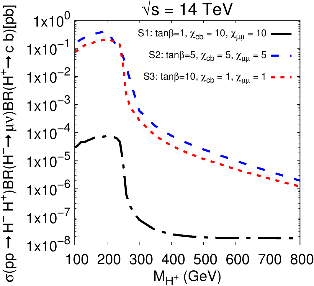
Meanwhile, we present in Fig. 13 the production cross-section of the signal as a function of charged scalar mass MH±subscript𝑀superscript𝐻plus-or-minusM_{H^{\pm}} for which we define three scenarios to be considered later, namely,

  • S1::𝑆1absentS1: tanβ=1𝛽1\tan\beta=1, χbc=χμμ=10subscript𝜒𝑏𝑐subscript𝜒𝜇𝜇10\chi_{bc}=\chi_{\mu\mu}=10 and cos(αβ)=0.01𝛼𝛽0.01\cos(\alpha-\beta)=0.01,

  • S2::𝑆2absentS2: tanβ=5𝛽5\tan\beta=5, χbc=χμμ=5subscript𝜒𝑏𝑐subscript𝜒𝜇𝜇5\chi_{bc}=\chi_{\mu\mu}=5 and cos(αβ)=0.01𝛼𝛽0.01\cos(\alpha-\beta)=0.01,

  • S3::𝑆3absentS3: tanβ=10𝛽10\tan\beta=10, χbc=χμμ=1subscript𝜒𝑏𝑐subscript𝜒𝜇𝜇1\chi_{bc}=\chi_{\mu\mu}=1 and cos(αβ)=0.01𝛼𝛽0.01\cos(\alpha-\beta)=0.01.

Refer to caption
Figure 13: Production cross-section of a charged Higgs pair with their subsequent decays into μνμcb𝜇subscript𝜈𝜇𝑐𝑏\mu\nu_{\mu}cb.

We observe for the three scenarios that the cross-sections are higher for masses in the range 100MH±250100subscript𝑀superscript𝐻plus-or-minus250100\leq M_{H^{\pm}}\leq 250 GeV. This is because there is an important contribution from the neutral heavy Higgs boson (MH=500GeV)subscript𝑀𝐻500GeV(M_{H}=500\,\rm GeV) which is capable of producing two real charged Higgs bosons. Once MH±=250GeVsubscript𝑀superscript𝐻plus-or-minus250GeVM_{H^{\pm}}=250\,\rm GeV, the mediation of H𝐻H is virtual, which suppresses the cross-section as MH±subscript𝑀superscript𝐻plus-or-minusM_{H^{\pm}} increases. It is worth mentioning that we chose MH=500GeVsubscript𝑀𝐻500GeVM_{H}=500\,\rm GeV motivated by the analysis of the parameter space carried out in Sec. III and by the scenarios that we have defined (S1S3)𝑆1𝑆3(S1-S3). We also find a high sensitivity on the χcbsubscript𝜒𝑐𝑏\chi_{cb}, χμμsubscript𝜒𝜇𝜇\chi_{\mu\mu} parameters which is reflected in a difference of up to 3 orders of magnitude in the cross-section by comparing the scenarios S1𝑆1S1 and S3𝑆3S3 (assuming MH±=250subscript𝑀superscript𝐻plus-or-minus250M_{H^{\pm}}=250 GeV). From Fig. 13 and Table 4, we note (in the most optimistic scenario, i.e., S2𝑆2S2 or S3𝑆3S3 and MH±200similar-tosubscript𝑀superscript𝐻plus-or-minus200M_{H^{\pm}}\sim 200 GeV) a difference of up to 4 orders of magnitude of the signal cross-section compared with the corresponding background production cross-section. This can be translated to a difference of 109superscript10910^{9} number of events assuming an integrated luminosity of 300300300 fb-1. In order to “isolate” the signal from the SM background, we perform a multivariate analysis, as described in Sec. IV.2.

As far as our computation scheme is concerned, we first implement the full model via FeynRules Alloul:2013bka for MadGraph5 MadGraphNLO , later it is interfaced with Pythia8 Sjostrand:2008vc and Delphes 3 delphes for detector simulations. Concerning the jet reconstruction, the finding package FastJet Cacciari:2011ma and the anti-ktsubscript𝑘𝑡k_{t} algorithm Cacciari:2008gp were used.

IV.2 Multivariate analysis

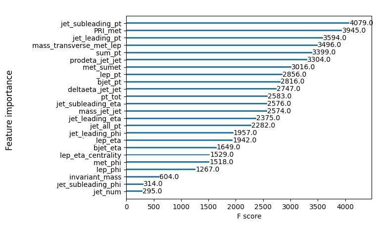
We compute a Boosted Decision Tree (BDT) training Woodruff2018 on the set variables shown in Fig. 14. On the same plot, we also present the most important ranking of the observables to separate the signal from the background, based on the F score.
Refer to caption
Figure 14: Importance ranking of several physical observables for a maximal tree depth of 10.

The five best-ranked observables shown in Fig. 14 are defined as follows:

  1. 1.

    jet_subleading_ptjet_subleading_pt\rm jet\_subleading\_pt = Jet with second largest transverse momentum,

  2. 2.

    PRI_metPRI_met\rm PRI\_met = Missing Energy Transverse (Tsubscriptitalic-E̸𝑇\not{E}_{T}),

  3. 3.

    jet_leading_ptjet_leading_pt\rm jet\_leading\_pt = Jet with largest transverse momentum,

  4. 4.

    mass_transverse_met_lepmass_transverse_met_lep\rm mass\_transverse\_met\_lep = Transverse mass between the MET and the lepton,

    MT(a, b)=(ax2+ay2+bx2+by2)2(ax+bx)2(ay+by)2,subscript𝑀𝑇a, bsuperscriptsuperscriptsubscript𝑎𝑥2superscriptsubscript𝑎𝑦2superscriptsubscript𝑏𝑥2superscriptsubscript𝑏𝑦22superscriptsubscript𝑎𝑥subscript𝑏𝑥2superscriptsubscript𝑎𝑦subscript𝑏𝑦2M_{T}(\textbf{a,\,b})=\sqrt{\Big{(}\sqrt{a_{x}^{2}+a_{y}^{2}}+\sqrt{b_{x}^{2}+b_{y}^{2}}\Big{)}^{2}-(a_{x}+b_{x})^{2}-(a_{y}+b_{y})^{2}},
  5. 5.

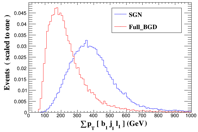
    sum_pt = Sum of the moduli of the transverse momentum of the b𝑏b-jet, leading jet and the muon μ𝜇\mu.

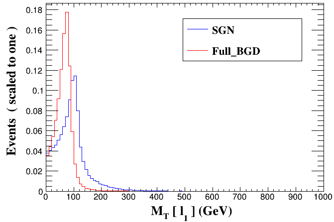
The rest of the definitions of the variables are presented in Appx. Definitions of observables. It is important to highlight that there is a relevant contribution coming from the production of the heavy neutral scalar boson H𝐻H predicted in the 2HDM-III. Its production is via gluon fusion with its subsequently decay into a charged scalar boson pair, which are produced as real particles if MH±<250subscript𝑀superscript𝐻plus-or-minus250M_{H^{\pm}}<250 GeV because we assume MH=500subscript𝑀𝐻500M_{H}=500 GeV. It is to be expected a final state with a high total transverse momentum (sum_pt) as shown in 16(e).

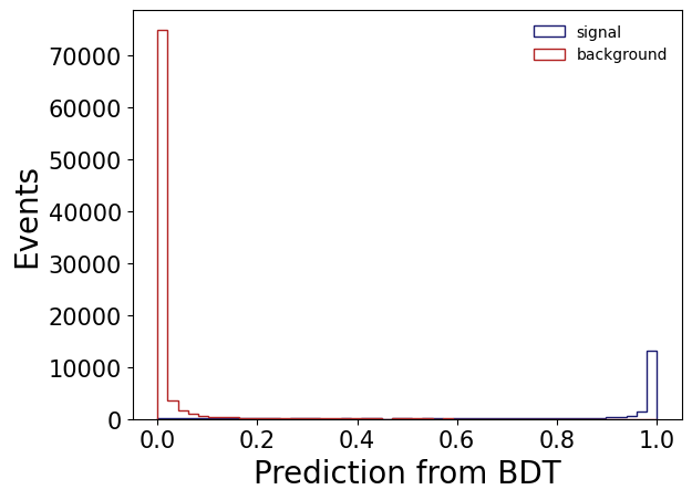
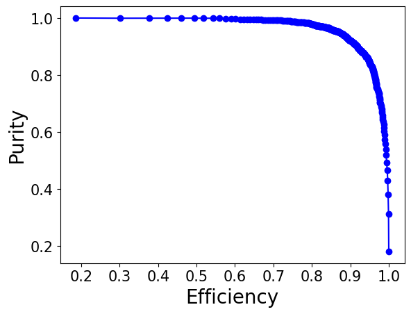
In the BDT training, the number of trees was set to 100 with a maximum depth of 10. Figure 15 shows the discriminant for the signal and background, which works very well. Meanwhile, a Receiver Operating Characteristic (ROC) curve of our analysis is presented in Fig. 15, where the efficiency is the number of events that are rightfully classified as signal divided by the number of events that are actually signal. The purity is the percentage of events in the whole test set that are rightfully classified as signal divided by the total number of events that have been classified as signal by the model. We note in these plots an excellent discrimination signal-background, which is reflected in the subsequent results.
Refer to caption
Refer to caption
Figure 15: (a) Plot of the discriminant for signal and background data. (b) ROC curve.

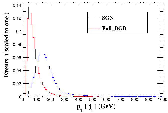
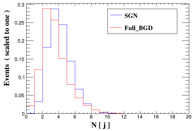
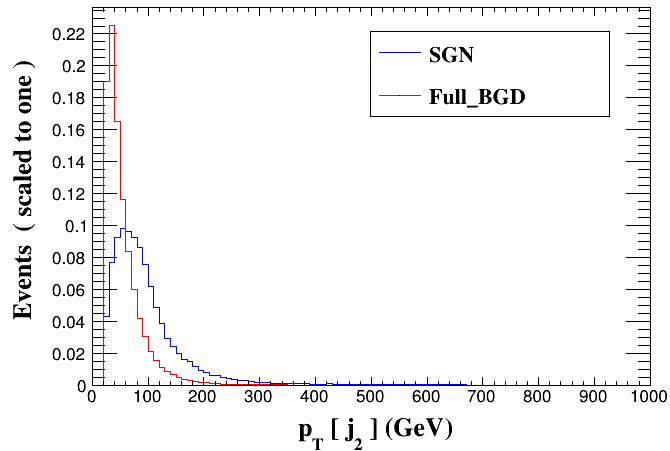
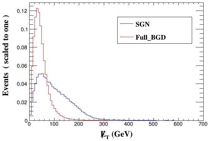
Figure 16 displays the distributions of the best-ranked observables by BDT. We also include a number of jets distribution.
Refer to caption
Refer to caption
Refer to caption
Refer to caption
Refer to caption
Refer to caption
Figure 16: Kinematic distributions of the signal and SM background processes: (a) transverse moment of the subleading jet, (b) missing energy transverse, (c) transverse moment of the leading jet, (d) transverse mass of the lepton, (e) sum of all transverse moment of the final state and (f) number of jets.

The previous analysis highly suggests imposing the following kinematic cuts:

  1. 1.

    PT[j2]>30subscript𝑃𝑇delimited-[]subscript𝑗230P_{T}[j_{2}]>30 GeV,

  2. 2.

    MET>20MET20\rm MET>20 GeV,

  3. 3.

    PT[j1]>30subscript𝑃𝑇delimited-[]subscript𝑗130P_{T}[j_{1}]>30 GeV,

  4. 4.

    MH±20<MT[μ]<MH±+20subscript𝑀superscript𝐻plus-or-minus20subscript𝑀𝑇delimited-[]𝜇subscript𝑀superscript𝐻plus-or-minus20M_{H^{\pm}}-20<M_{T}[\mu]<M_{H^{\pm}}+20 GeV,

  5. 5.

    PT>120subscript𝑃𝑇120\sum P_{T}>120 GeV.

Signal significance

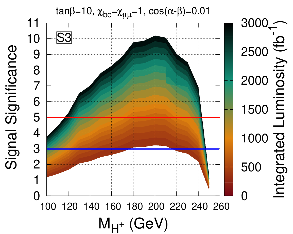
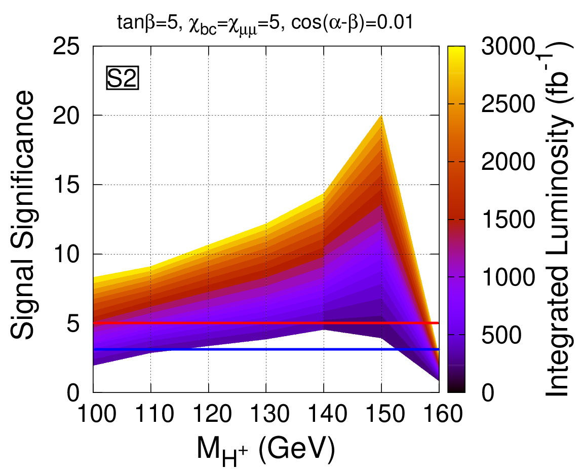
We present the our most important results concerning to a potential evidence/discovery for the process ppH+Hμνμcb𝑝𝑝superscript𝐻superscript𝐻𝜇subscript𝜈𝜇𝑐𝑏pp\to H^{+}H^{-}\to\mu\nu_{\mu}cb. The signal significance considered here is defined as the ratio 𝒩S/𝒩S+𝒩Bsubscript𝒩𝑆subscript𝒩𝑆subscript𝒩𝐵\mathcal{N}_{S}/\sqrt{\mathcal{N}_{S}+\mathcal{N}_{B}}, where 𝒩S(𝒩B)subscript𝒩𝑆subscript𝒩𝐵\mathcal{N}_{S}\,(\mathcal{N}_{B}) is the number of signal (background) events once the kinematic cuts were applied. We use the package MadAnalysis5 Conte:2012fm to analyze the kinematic distributions. Figure 17 displays contour plots of the signal significance as function of the charged Higgs boson mass MH±subscript𝑀superscript𝐻plus-or-minusM_{H^{\pm}} and the integrated luminosity for the scenarios S2𝑆2S2444We explore up to MH±=200subscript𝑀superscript𝐻plus-or-minus200M_{H^{\pm}}=200 GeV, however we found a tiny signal significance. and S3𝑆3S3. We find that the scenario S1𝑆1S1 presents difficulties to be tested in the experiment, which is why it is not included.
Refer to caption
Refer to caption
Figure 17: Signal significance as function of of the charged Higgs boson mass and the integrated luminosity for (a) S2𝑆2S2, (b) S3𝑆3S3. Red (Blue) line indicates a potential discovery (evidence).

We have found two very promising scenarios for experimental exploration. For S2𝑆2S2 we predict a statistical significance of 3σ3𝜎3\sigma in the 100MH±160100subscript𝑀superscript𝐻plus-or-minus160100\leq M_{H^{\pm}}\leq 160 GeV interval corresponding to an integrated luminosity in the range 300500300500300-500 fb-1. An interesting interval is 115MH±155less-than-or-similar-to115subscript𝑀superscript𝐻plus-or-minusless-than-or-similar-to155115\lesssim M_{H^{\pm}}\lesssim 155 GeV, for which evidence or excess events could be declared accumulating around 250 fb-1 at the LHC. The same scenario S2𝑆2S2 offers the possibility of a potential discovery if the integrated luminosity is increased to at least 800similar-toabsent800\sim 800 fb-1 for 115MH±140less-than-or-similar-to115subscript𝑀superscript𝐻plus-or-minusless-than-or-similar-to140115\lesssim M_{H^{\pm}}\lesssim 140 GeV. However, to cover the full range 100MH±160100subscript𝑀superscript𝐻plus-or-minus160100\leq M_{H^{\pm}}\leq 160 GeV, an integrated luminosity in the range 800800800 to 240024002400 fb-1 is necessary. Concerning scenario S3𝑆3S3, it also has the potential to be brought to experimental scrutiny, even explore up to MH±=250subscript𝑀superscript𝐻plus-or-minus250M_{H^{\pm}}=250 GeV. We foretell a statistical signal of 3σ3𝜎3\sigma for 100MH±250less-than-or-similar-to100subscript𝑀superscript𝐻plus-or-minusless-than-or-similar-to250100\lesssim M_{H^{\pm}}\lesssim 250 GeV corresponding to 30030003003000300-3000 fb-1 of the accumulated data. As in the previous scenario (S2𝑆2S2), the LHC has the potential to search for evidence of the proposed signal once it accumulates around 280280280 fb-1. Meanwhile, we need to achieve accumulated data around 300030003000 fb-1 to declare a potential discovery of a charged Higgs boson with masses between 120MH±250less-than-or-similar-to120subscript𝑀superscript𝐻plus-or-minusless-than-or-similar-to250120\lesssim M_{H^{\pm}}\lesssim 250 GeV.

V Conclusions

In this work, we have explored the production and the possible detection of a charged scalar boson predicted in an extension of the Standard Model, the so-called Two-Higgs Doublet Model of type III. The production channel studied is via simulated proton-proton collisions for the LHC and the HL-LHC, that is, ppHH+μνμcb𝑝𝑝superscript𝐻superscript𝐻𝜇subscript𝜈𝜇𝑐𝑏pp\to H^{-}H^{+}\to\mu\nu_{\mu}cb. Through deep analysis of the model parameter space, we found very promising benchmarks that could be tested in forthcoming runs at the LHC and its next step, the HL-LHC. Specifically, we identify two valuable scenarios, S2:tanβ=χμμ=χcb=5,cos(αβ)=0.01S2:\,\tan\beta=\chi_{\mu\mu}=\chi_{cb}=5,\,\cos(\alpha-\beta)=0.01 and S3:tanβ=10,χμμ=χcb=1,cos(αβ)=0.01S3:\,\tan\beta=10,\,\chi_{\mu\mu}=\chi_{cb}=1,\,\cos(\alpha-\beta)=0.01. Once integrated luminosities from 800similar-toabsent800\sim 800 fb-1 to 300030003000 fb-1 and 1000similar-toabsent1000\sim 1000 fb-1 to 300030003000 fb-1 are reached, we predict a signal significance of 5σ5𝜎5\sigma for the intervals 110MH±160less-than-or-similar-to110subscript𝑀superscript𝐻plus-or-minusless-than-or-similar-to160110\lesssim M_{H^{\pm}}\lesssim 160 and 120MH±250less-than-or-similar-to120subscript𝑀superscript𝐻plus-or-minusless-than-or-similar-to250120\lesssim M_{H^{\pm}}\lesssim 250, respectively. Furthermore, according to our analysis, the LHC has the potential to search for evidence of the proposed signal for 115MH±155less-than-or-similar-to115subscript𝑀superscript𝐻plus-or-minusless-than-or-similar-to155115\lesssim M_{H^{\pm}}\lesssim 155 and 120MH±240less-than-or-similar-to120subscript𝑀superscript𝐻plus-or-minusless-than-or-similar-to240120\lesssim M_{H^{\pm}}\lesssim 240 if it achieves around 250250250 and 280280280 fb-1 of the accumulated data for S2𝑆2S2 and S3𝑆3S3, respectively.

Acknowledgments

The work of M. A. Arroyo-Ureña is supported by “Estancias posdoctorales por México (CONAHCYT)” and “Sistema Nacional de Investigadores” (SNI-CONAHCYT). S. Rosado-Navarro thanks to Vicerrectoría de Investigación y Estudios de Posgrado through “Centro Interdisciplinario de Investigación y enseñanza de la Ciencia”. E. A. Herrera-Chacón acknowledges support from CONAHCYT.

Appendix V

Constraints

We present individual allowed regions by different constraints for each observable described in Sec. III, namely,

  • Signal strengths

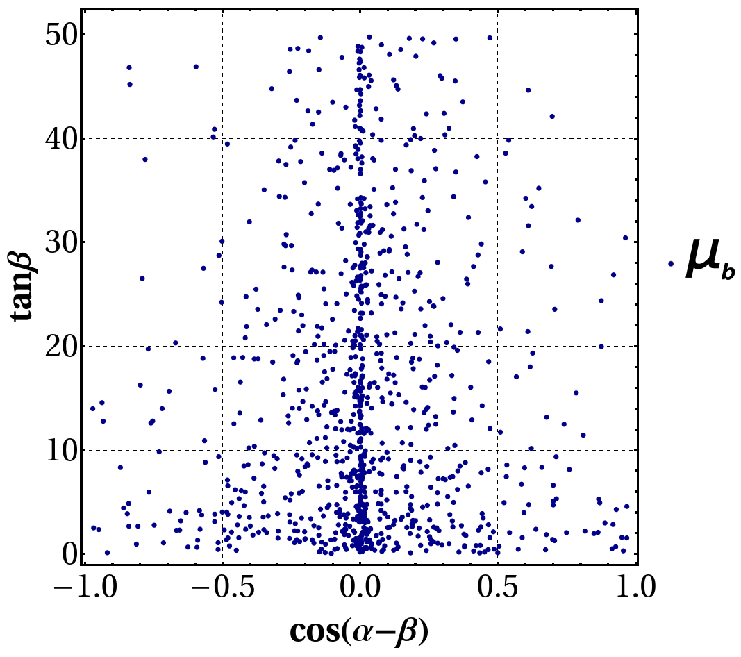
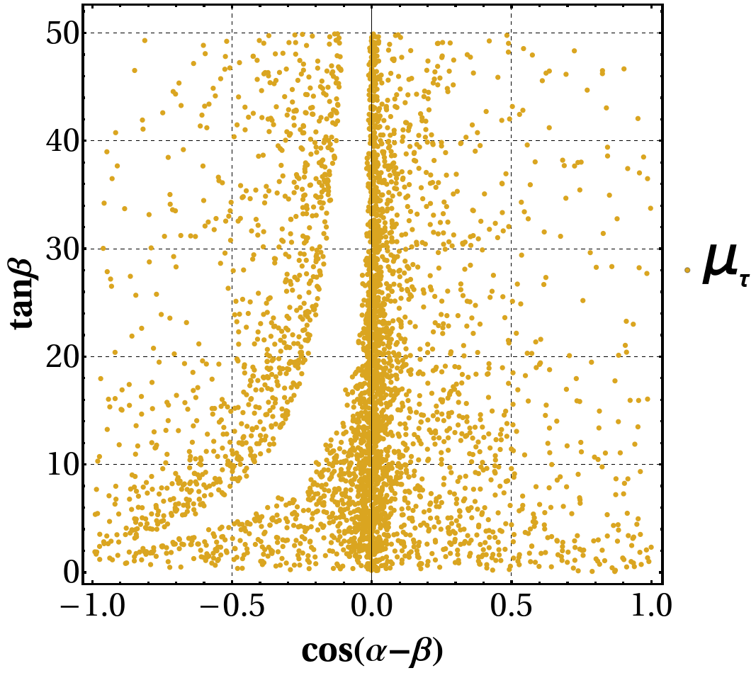
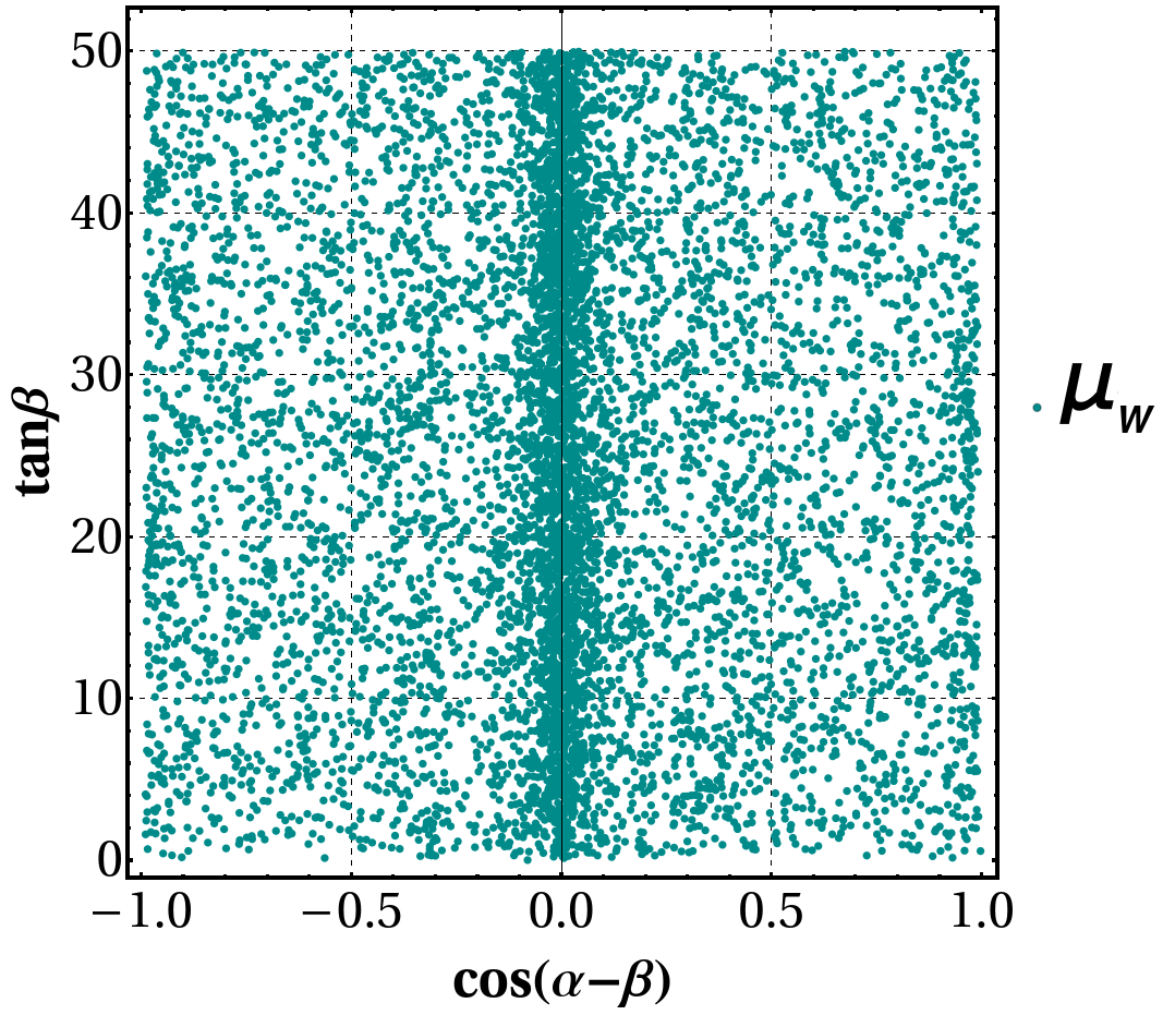
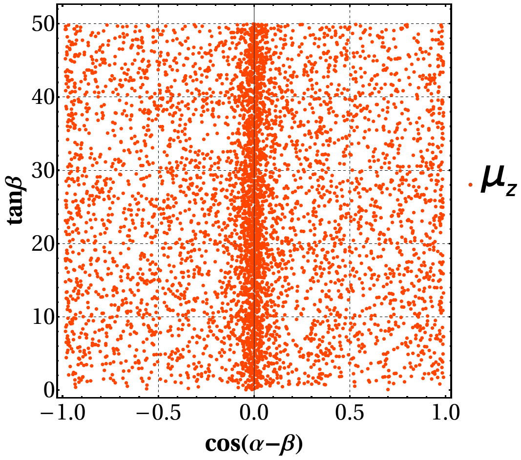
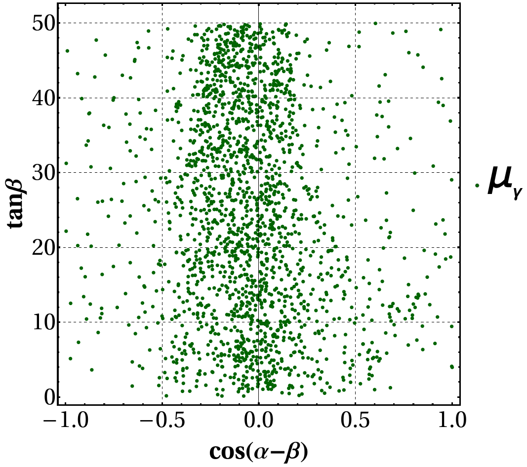
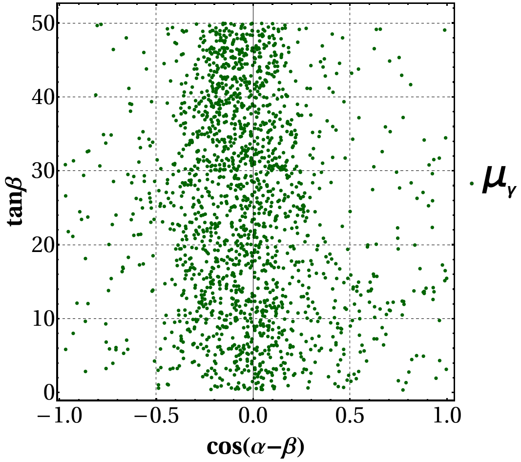
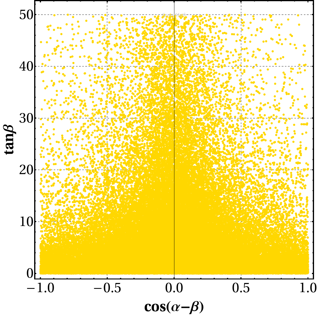
We present in Fig. 18 individual cos(αβ)tanβ𝛼𝛽𝛽\cos(\alpha-\beta)-\tan\beta planes associated to each μXsubscript𝜇𝑋\mu_{X}. The colored points correspond to those allowed by μXsubscript𝜇𝑋\mu_{X}. While Tab. 5 shows the range of scanned parameters involved in the evaluation of the signal strengths μXsubscript𝜇𝑋\mu_{X}.

Refer to caption
Refer to caption
Refer to caption
Refer to caption
Refer to caption
Refer to caption
Figure 18: Signal strengths: (a) μbsubscript𝜇𝑏\mu_{b}, (b) μτsubscript𝜇𝜏\mu_{\tau}, (c) μWsubscript𝜇𝑊\mu_{W}, (d) μZsubscript𝜇𝑍\mu_{Z}, (e) μγsubscript𝜇𝛾\mu_{\gamma} (114MH±140114subscript𝑀superscript𝐻plus-or-minus140114\leq M_{H^{\pm}}\leq 140), (d) μγsubscript𝜇𝛾\mu_{\gamma} (mt+mbMH±1000subscript𝑚𝑡subscript𝑚𝑏subscript𝑀superscript𝐻plus-or-minus1000m_{t}+m_{b}\leq M_{H^{\pm}}\leq 1000). In all cases we generate 505050K random points.
Table 5: Range of scanned parameters for the signal strengths μX.subscript𝜇𝑋\mu_{X}.
Parameter Range
tanβ𝛽\tan\beta [0,50]050[0,50]
cos(αβ)𝛼𝛽\cos(\alpha-\beta) [1,1]11[-1,1]
χbbsubscript𝜒𝑏𝑏\chi_{bb} [1,1]11[-1,1]
χttsubscript𝜒𝑡𝑡\chi_{tt} [100,100]100100[-100,100]
χττsubscript𝜒𝜏𝜏\chi_{\tau\tau} [1,1]11[-1,1]
MH±subscript𝑀superscript𝐻plus-or-minusM_{H^{\pm}} (GeV) [114,140]114140[114,140]
MH±subscript𝑀superscript𝐻plus-or-minusM_{H^{\pm}} (GeV) [mt+mb,1000]subscript𝑚𝑡subscript𝑚𝑏1000[m_{t}+m_{b},1000]
  • Decays Bs,d0μ+μsuperscriptsubscript𝐵𝑠𝑑0superscript𝜇superscript𝜇B_{s,d}^{0}\to\mu^{+}\mu^{-}

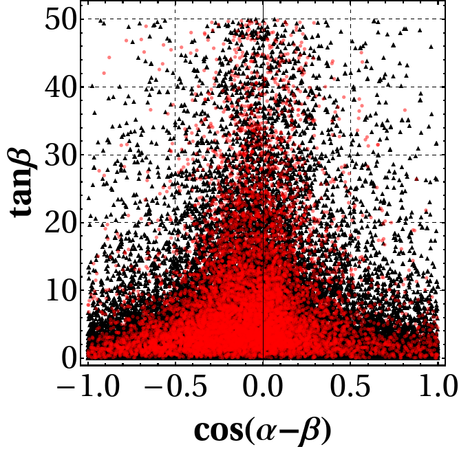
Fig. 19 presents the allowed points by experimental measurements on (Bs,d0μ+μ)superscriptsubscript𝐵𝑠𝑑0superscript𝜇superscript𝜇\mathcal{BR}(B_{s,d}^{0}\to\mu^{+}\mu^{-}). The range of scanned parameters is displayed in Table 6.
Refer to caption
Figure 19: Allowed values by the measurement on (Bd0μ+μ)superscriptsubscript𝐵𝑑0superscript𝜇superscript𝜇\mathcal{BR}(B_{d}^{0}\to\mu^{+}\mu^{-}) (black triangles) and by the upper limit on (Bs0μ+μ)superscriptsubscript𝐵𝑠0superscript𝜇superscript𝜇\mathcal{BR}(B_{s}^{0}\to\mu^{+}\mu^{-}) (light red circles). In both cases we generate 505050K random points.
Table 6: Range of scanned parameters. On the left: Bd0μ+μsuperscriptsubscript𝐵𝑑0superscript𝜇superscript𝜇B_{d}^{0}\to\mu^{+}\mu^{-}, on the right: Bs0μ+μsuperscriptsubscript𝐵𝑠0superscript𝜇superscript𝜇B_{s}^{0}\to\mu^{+}\mu^{-}
Parameter Range
tanβ𝛽\tan\beta [0,50]050[0,50]
cos(αβ)𝛼𝛽\cos(\alpha-\beta) [1,1]11[-1,1]
χμμsubscript𝜒𝜇𝜇\chi_{\mu\mu} [1,1]11[-1,1]
χbdsubscript𝜒𝑏𝑑\chi_{bd} [1,1]11[-1,1]
χdbsubscript𝜒𝑑𝑏\chi_{db} [1,1]11[-1,1]
MAsubscript𝑀𝐴M_{A} (GeV) [100,1000]1001000[100,1000]
MHsubscript𝑀𝐻M_{H} (GeV) [300,1000]3001000[300,1000]

       Parameter Range tanβ𝛽\tan\beta [0,50]050[0,50] cos(αβ)𝛼𝛽\cos(\alpha-\beta) [1,1]11[-1,1] χμμsubscript𝜒𝜇𝜇\chi_{\mu\mu} [1,1]11[-1,1] χbssubscript𝜒𝑏𝑠\chi_{bs} [1,1]11[-1,1] χsbsubscript𝜒𝑠𝑏\chi_{sb} [1,1]11[-1,1] MAsubscript𝑀𝐴M_{A} (GeV) [100,1000]1001000[100,1000] MHsubscript𝑀𝐻M_{H} (GeV) [300,1000]3001000[300,1000]

  • ijγsubscript𝑖subscript𝑗𝛾\ell_{i}\to\ell_{j}\gamma

Fig. 20 shows the corresponding allowed points that meet upper limits on (ijγ)subscript𝑖subscript𝑗𝛾\mathcal{BR}(\ell_{i}\to\ell_{j}\gamma). The range of scanned parameters is displayed in Table 7.
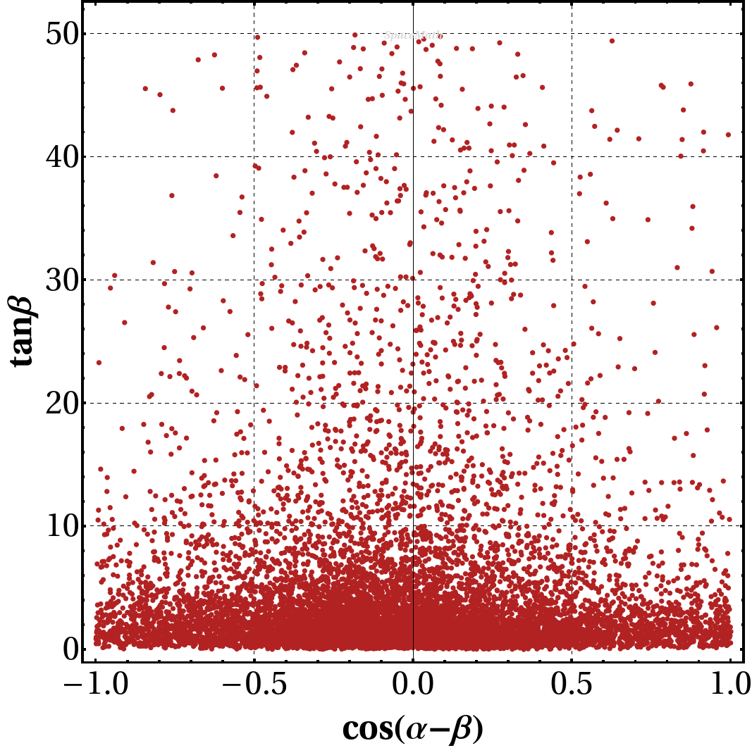
Refer to caption
Refer to caption
Refer to caption
Figure 20: Decays ijγsubscript𝑖subscript𝑗𝛾\ell_{i}\to\ell_{j}\gamma: (a) μeγ𝜇𝑒𝛾\mu\to e\gamma, (b) τμγ𝜏𝜇𝛾\tau\to\mu\gamma, (c) τeγ𝜏𝑒𝛾\tau\to e\gamma. In all cases we generate 100100100K random points.
Table 7: Range of scanned parameters. On the left: μeγ𝜇𝑒𝛾\mu\to e\gamma, on the center: τμγ𝜏𝜇𝛾\tau\to\mu\gamma on the right: τeγ𝜏𝑒𝛾\tau\to e\gamma
Parameter Range
tanβ𝛽\tan\beta [0,50]050[0,50]
cos(αβ)𝛼𝛽\cos(\alpha-\beta) [1,1]11[-1,1]
χμμsubscript𝜒𝜇𝜇\chi_{\mu\mu} [1,1]11[-1,1]
χμesubscript𝜒𝜇𝑒\chi_{\mu e} [1,1]11[-1,1]
χttsubscript𝜒𝑡𝑡\chi_{tt} [100,100]100100[-100,100]
MAsubscript𝑀𝐴M_{A} (GeV) [100,1000]1001000[100,1000]
MHsubscript𝑀𝐻M_{H} (GeV) [300,1000]3001000[300,1000]
MH±subscript𝑀superscript𝐻plus-or-minusM_{H^{\pm}} (GeV) [110,1000]1101000[110,1000]

       Parameter Range tanβ𝛽\tan\beta [0,50]050[0,50] cos(αβ)𝛼𝛽\cos(\alpha-\beta) [1,1]11[-1,1] χτμsubscript𝜒𝜏𝜇\chi_{\tau\mu} [100,100]100100[-100,100] χττsubscript𝜒𝜏𝜏\chi_{\tau\tau} [1,1]11[-1,1] χttsubscript𝜒𝑡𝑡\chi_{tt} [100,100]100100[-100,100] MAsubscript𝑀𝐴M_{A} (GeV) [100,1000]1001000[100,1000] MHsubscript𝑀𝐻M_{H} (GeV) [300,1000]3001000[300,1000] MH±subscript𝑀superscript𝐻plus-or-minusM_{H^{\pm}} (GeV) [110,1000]1101000[110,1000]        Parameter Range tanβ𝛽\tan\beta [0,50]050[0,50] cos(αβ)𝛼𝛽\cos(\alpha-\beta) [1,1]11[-1,1] χτesubscript𝜒𝜏𝑒\chi_{\tau e} [1,1]11[-1,1] χττsubscript𝜒𝜏𝜏\chi_{\tau\tau} [1,1]11[-1,1] χttsubscript𝜒𝑡𝑡\chi_{tt} [100,100]100100[-100,100] MAsubscript𝑀𝐴M_{A} (GeV) [100,1000]1001000[100,1000] MHsubscript𝑀𝐻M_{H} (GeV) [300,1000]3001000[300,1000] MH±subscript𝑀superscript𝐻plus-or-minusM_{H^{\pm}} (GeV) [110,1000]1101000[110,1000]

  • Decays ijk¯ksubscript𝑖subscript𝑗subscript𝑘subscript¯𝑘\ell_{i}\to\ell_{j}\ell_{k}\bar{\ell}_{k}

As far as the decays ijk¯ksubscript𝑖subscript𝑗subscript𝑘subscript¯𝑘\ell_{i}\to\ell_{j}\ell_{k}\bar{\ell}_{k} are concerned, we present in Fig. 21 the points that comply with the constraints on (ijk¯k)subscript𝑖subscript𝑗subscript𝑘subscript¯𝑘\mathcal{BR}(\ell_{i}\to\ell_{j}\ell_{k}\bar{\ell}_{k}). And in Table 8 the intervals of the scan on the parameters are presented.
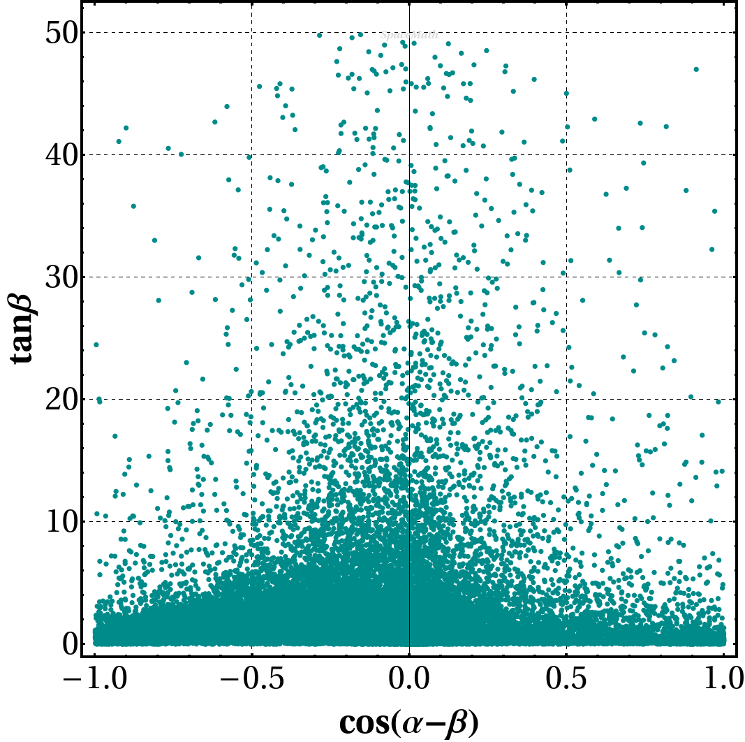
Refer to caption
Refer to caption
Figure 21: Decays ijk¯ksubscript𝑖subscript𝑗subscript𝑘subscript¯𝑘\ell_{i}\to\ell_{j}\ell_{k}\bar{\ell}_{k}: (a) μ3e𝜇3𝑒\mu\to 3e, (b) τ3μ𝜏3𝜇\tau\to 3\mu). In all cases we generate 100100100K random points.
Table 8: Range of scanned parameters. On the left: μ3e𝜇3𝑒\mu\to 3e, on the right: τ3μ𝜏3𝜇\tau\to 3\mu.
Parameter Range
tanβ𝛽\tan\beta [0,50]050[0,50]
cos(αβ)𝛼𝛽\cos(\alpha-\beta) [1,1]11[-1,1]
χeesubscript𝜒𝑒𝑒\chi_{ee} [1,1]11[-1,1]
χμesubscript𝜒𝜇𝑒\chi_{\mu e} [1,1]11[-1,1]
MAsubscript𝑀𝐴M_{A} (GeV) [100,1000]1001000[100,1000]
MHsubscript𝑀𝐻M_{H} (GeV) [300,1000]3001000[300,1000]

       Parameter Range tanβ𝛽\tan\beta [0,50]050[0,50] cos(αβ)𝛼𝛽\cos(\alpha-\beta) [1,1]11[-1,1] χμμsubscript𝜒𝜇𝜇\chi_{\mu\mu} [1,1]11[-1,1] χτμsubscript𝜒𝜏𝜇\chi_{\tau\mu} [100,100]100100[-100,100] MAsubscript𝑀𝐴M_{A} (GeV) [100,1000]1001000[100,1000] MHsubscript𝑀𝐻M_{H} (GeV) [300,1000]3001000[300,1000]

  • Decays hijsubscript𝑖subscript𝑗h\to\ell_{i}\ell_{j}

We only present the allowed region coming from hτμ𝜏𝜇h\to\tau\mu because the process heμ𝑒𝜇h\to e\mu imposes very weak bounds to tanβ𝛽\tan\beta and cos(αβ)𝛼𝛽\cos(\alpha-\beta). Fig. 22 presents the scatter plot in the cos(αβ)tanβ𝛼𝛽𝛽\cos(\alpha-\beta)-\tan\beta plane whose points are the allowed by the upper limit on (hτμ)𝜏𝜇\mathcal{BR}(h\to\tau\mu).

Refer to caption
Figure 22: Allowed values by the upper limit on (hτμ)𝜏𝜇\mathcal{BR}(h\to\tau\mu). We generate 505050K random points.

The range of scanned parameters is displayed in Table 9.

Table 9: Range of scanned parameters associated to the decay hτμ𝜏𝜇h\to\tau\mu.
Parameter Range
tanβ𝛽\tan\beta [0,50]050[0,50]
cos(αβ)𝛼𝛽\cos(\alpha-\beta) [1,1]11[-1,1]
χτμsubscript𝜒𝜏𝜇\chi_{\tau\mu} [10,10]1010[-10,10]

Definitions of observables

  1. 1.

    prodeta_jet_jet = Product of the pseudorapidities of the two jets.

  2. 2.

    met_sumet = Total transverse energy in the detector.

  3. 3.

    _lep_pt = Lepton transverse momentum.

  4. 4.

    bjet_pt = Bjet transverse momentum.

  5. 5.

    deltaeta_jet_jet = Absolute value of the pseudorapidity separation between two jets. |ηjet2ηjet1|subscript𝜂jet2subscript𝜂jet1|\eta_{\text{jet2}}-\eta_{\text{jet1}}|

  6. 6.

    pt_tot = Modulus of the vector sum of the missing transverse momenta and the transverse momenta of the hadronic tau, the lepton, the leading jet, and the subleading jet.

  7. 7.

    jet_subleading_eta = Subleading jet pseudorapidity η𝜂\eta.

  8. 8.

    mass_jet_jet = Invariant mass of the leading and subleading jets.
    2pt jet1pt jet2(cosh(ηjet1ηjet2)cos(ϕjet1ϕjet1))2subscript𝑝t jet1subscript𝑝t jet2subscript𝜂jet1subscript𝜂jet2subscriptitalic-ϕjet1subscriptitalic-ϕjet1\sqrt{2\cdot p_{\text{t jet1}}\cdot p_{\text{t jet2}}\cdot\left(\cosh(\eta_{\text{jet1}}-\eta_{\text{jet2}})-\cos(\phi_{\text{jet1}}-\phi_{\text{jet1}})\right)}

  9. 9.

    jet_leading_eta = Leading jet pseudorapidity η𝜂\eta.

  10. 10.

    jet_all_pt = Scalar sum of the transverse momentum of all the jets of the events.

  11. 11.

    jet_leading_phi = Leading jet azimuth angle ϕitalic-ϕ\phi.

  12. 12.

    lep_eta = Pseudorapidity η𝜂\eta of the lepton.

  13. 13.

    bjet_eta = Pseudorapidity η𝜂\eta of the bjet.

  14. 14.

    lep_eta_centrality = Centrality of the pseudorapidity of the lepton w.r.t. the two jets. exp[(4(n1n2)2)(nlep(η1+η2)2)2]4superscript𝑛1𝑛22superscriptsubscript𝑛lepsubscript𝜂1subscript𝜂222\exp\left[-\left(\frac{4}{(n1-n2)^{2}}\right)\left(n_{\text{lep}}-\frac{(\eta_{1}+\eta_{2})}{2}\right)^{2}\right], where nlepsubscript𝑛lepn_{\text{lep}} is the pseudorapidity of the lepton and η1subscript𝜂1\eta_{1} and η2subscript𝜂2\eta_{2} are the pseudorapidities of the two jets.

  15. 15.

    met_phi = Azimuth angle ϕitalic-ϕ\phi of the missing transverse energy.

  16. 16.

    lep_phi = Azimuth angle ϕitalic-ϕ\phi of the lepton.

  17. 17.

    invariant_mass = Invariant mass of the bjet and cjet.

  18. 18.

    jet_subleading_phi = Azimuth angle ϕitalic-ϕ\phi of the subleading jet.

  19. 19.

    jet_num = Number of jets.

References

  • (1) G. Aad et al. [ATLAS], Phys. Rev. D 108 (2023) no.9, 092007 doi:10.1103/PhysRevD.108.092007 [arXiv:2304.14247 [hep-ex]].
  • (2) G. Aad et al. [ATLAS], JHEP 06 (2012), 039 doi:10.1007/JHEP06(2012)039 [arXiv:1204.2760 [hep-ex]].
  • (3) S. Chatrchyan et al. [CMS], JHEP 07 (2012), 143 doi:10.1007/JHEP07(2012)143 [arXiv:1205.5736 [hep-ex]].
  • (4) G. Aad et al. [ATLAS], JHEP 09 (2023), 004 doi:10.1007/JHEP09(2023)004 [arXiv:2302.11739 [hep-ex]].
  • (5) J. Hernández-Sánchez, C. G. Honorato, S. Moretti and S. Rosado-Navarro, Phys. Rev. D 102, no.5, 055008 (2020) doi:10.1103/PhysRevD.102.055008 [arXiv:2003.06263 [hep-ph]].
  • (6) O. Félix-Beltrán, F. González-Canales, J. Hernández-Sánchez, S. Moretti, R. Noriega-Papaqui and A. Rosado, Phys. Lett. B 742, 347 (2015) [arXiv:1311.5210 [hep-ph]].
  • (7) J. Hernández-Sánchez, S. Moretti, R. Noriega-Papaqui and A. Rosado, JHEP 1307, 044 (2013) [arXiv:1212.6818 [hep-ph]].
  • (8) M. A. Arroyo-Ureña, T. A. Valencia-Pérez, R. Gaitán, J. H. Montes De Oca and A. Fernández-Téllez, JHEP 08 (2020), 170 doi:10.1007/JHEP08(2020)170 [arXiv:2002.04120 [hep-ph]].
  • (9) M. A. Arroyo-Ureña, R. Gaitán, E. A. Herrera-Chacón, J. H. Montes de Oca Y. and T. A. Valencia-Pérez, JHEP 07 (2019), 041 doi:10.1007/JHEP07(2019)041 [arXiv:1903.02718 [hep-ph]].
  • (10) M. A. Arroyo-Ureña, J. L. Diaz-Cruz, E. Díaz and J. A. Orduz-Ducuara, Chin. Phys. C 40 (2016) no.12, 123103 doi:10.1088/1674-1137/40/12/123103 [arXiv:1306.2343 [hep-ph]].
  • (11) A. M. Sirunyan et al. [CMS], JHEP 06 (2018), 001 doi:10.1007/JHEP06(2018)001 [arXiv:1712.07173 [hep-ex]].
  • (12) G. Aad et al. [ATLAS], Phys. Lett. B 800 (2020), 135069 doi:10.1016/j.physletb.2019.135069 [arXiv:1907.06131 [hep-ex]].
  • (13) A. Tumasyan et al. [CMS], Phys. Lett. B 842 (2023), 137955 doi:10.1016/j.physletb.2023.137955 [arXiv:2212.10311 [hep-ex]].
  • (14) R. L. Workman et al. [Particle Data Group], PTEP 2022, 083C01 (2022) doi:10.1093/ptep/ptac097
  • (15) B. Abi et al. [Muon g-2], Phys. Rev. Lett. 126 (2021) no.14, 141801 doi:10.1103/PhysRevLett.126.141801 [arXiv:2104.03281 [hep-ex]].
  • (16) G. Aad et al. [ATLAS], Phys. Rev. D 106 (2022) no.5, 052001 doi:10.1103/PhysRevD.106.052001 [arXiv:2112.11876 [hep-ex]].
  • (17) ATLAS Collaboration, CERN Report No. ATLAS-CONF-2017-055, 2017.
  • (18) A. M. Sirunyan et al. [CMS Collaboration], JHEP 1809, 007 (2018) doi:10.1007/JHEP09(2018)007 [arXiv:1803.06553 [hep-ex]].
  • (19) M. Aaboud et al. [ATLAS], JHEP 09 (2018), 139 doi:10.1007/JHEP09(2018)139 [arXiv:1807.07915 [hep-ex]].
  • (20) M. Ciuchini, G. Degrassi, P. Gambino and G. F. Giudice, Nucl. Phys. B 527, 21 (1998) doi:10.1016/S0550-3213(98)00244-2 [hep-ph/9710335].
  • (21) M. Misiak and M. Steinhauser, Eur. Phys. J. C 77, no. 3, 201 (2017) doi:10.1140/epjc/s10052-017-4776-y [arXiv:1702.04571 [hep-ph]].
  • (22) M. Beneke, C. Bobeth and R. Szafron, JHEP 10 (2019), 232 [erratum: JHEP 11 (2022), 099] doi:10.1007/JHEP10(2019)232 [arXiv:1908.07011 [hep-ph]].
  • (23) A. J. Buras, J. Girrbach, D. Guadagnoli and G. Isidori, Eur. Phys. J. C 72 (2012), 2172 doi:10.1140/epjc/s10052-012-2172-1 [arXiv:1208.0934 [hep-ph]].
  • (24) T. Inami and C. S. Lim, Prog. Theor. Phys. 65 (1981), 297 [erratum: Prog. Theor. Phys. 65 (1981), 1772] doi:10.1143/PTP.65.297
  • (25) R. Harnik, J. Kopp and J. Zupan, JHEP 03 (2013), 026 doi:10.1007/JHEP03(2013)026 [arXiv:1209.1397 [hep-ph]].
  • (26) G. Blankenburg, J. Ellis and G. Isidori, Phys. Lett. B 712 (2012), 386-390 doi:10.1016/j.physletb.2012.05.007 [arXiv:1202.5704 [hep-ph]].
  • (27) M. A. Arroyo-Ureña, R. Gaitán and T. A. Valencia-Pérez, Rev. Mex. Fis. E 19 (2022) no.2, 020206 doi:10.31349/RevMexFisE.19.020206 [arXiv:2008.00564 [hep-ph]].
  • (28) A. Alloul, N. D. Christensen, C. Degrande, C. Duhr and B. Fuks, Comput. Phys. Commun. 185 (2014), 2250-2300 doi:10.1016/j.cpc.2014.04.012 [arXiv:1310.1921 [hep-ph]].
  • (29) J. Alwall, M. Herquet, F. Maltoni, O. Mattelaer, and T.Stelzer, J. High Energy Phys. 06 (2011) 128.
  • (30) T. Sjostrand, doi:10.3204/DESY-PROC-2009-02/41 arXiv:0809.0303 [hep-ph].
  • (31) J. de Favereau, C. Delaere, P. Demin, A. Giammanco, V. Lemaitre, A. Mertens, and M. Selvaggi, J. High Energy Phys. 02 (2014) 057.
  • (32) M. Cacciari, G. P. Salam and G. Soyez, Eur. Phys. J. C 72 (2012), 1896 doi:10.1140/epjc/s10052-012-1896-2 [arXiv:1111.6097 [hep-ph]].
  • (33) M. Cacciari, G. P. Salam and G. Soyez, JHEP 04 (2008), 063 doi:10.1088/1126-6708/2008/04/063 [arXiv:0802.1189 [hep-ph]].
  • (34) K. Woodruff, GitHub repository (2018), https://github.com/k-woodruff/bdt-tutorial
  • (35) E. Conte, B. Fuks and G. Serret, Comput. Phys. Commun. 184 (2013), 222-256 doi:10.1016/j.cpc.2012.09.009 [arXiv:1206.1599 [hep-ph]].