Primitive Quantum Gates for an $SU(3)$ Discrete Subgroup: $\Sigma(36\times 3)$

Abstract

We construct the primitive gate set for the digital quantum simulation of the 108-element $\Sigma(36\times 3)$ group. This is the first time a nonabelian crystal-like subgroup of $SU(3)$ has been constructed for quantum simulation. The gauge link registers and necessary primitives – the inversion gate, the group multiplication gate, the trace gate, and the $\Sigma(36\times 3)$ Fourier transform – are presented for both an eight-qubit encoding and a heterogeneous three-qutrit plus two-qubit register. For the latter, a specialized compiler was developed for decomposing arbitrary unitaries onto this architecture.

I Introduction

Classical computers face significant challenges in simulating lattice gauge theories due to inherent exponentially large Hilbert spaces with the lattice volume. Monte Carlo simulations in Euclidean time are generally used to circumvent this problem. However, this approach also fails when we are interested in the real time dynamics of the system or in the properties of matter at finite density due to the sign problem [1, 2, 3, 4, 5, 6, 7, 8].

Quantum computers provide a natural way of simulating lattice gauge theories. Yet, they are currently limited to a small number of qubits and circuit depths. Gauge theories contain bosonic degrees of freedom and have a continuous symmetry, e.g. Quantum chromodynamics (QCD) with $SU(3)$ local symmetry. Storing a faithful matrix representation of $SU(3)$ to double precision would require $\mathcal{O}(10^{3})$ qubits per link – far beyond accessibility to near-term quantum computers. Moreover, these qubits being noisy significantly limits the circuit depths that can be reliably performed on these devices. Therefore, studying lattice gauge theories with current and near-future quantum computers requires efficient digitization methods of gauge fields as well as optimized computational subroutines. Finally, it is important to note that a choice of digitization method affects the computation cost.

To this end, several digitization methods have been proposed in the past decade to render the bosonic Hilbert space finite. Traditionally, most approaches have considered only qubit devices. However, due to recent demonstrations demonstration of qudit gates, there has been an increasing interest in qudit-based digitization methods [9, 10, 11, 12, 13, 14, 15, 16]. One digitization method utilizes the representation (electric field) basis, and impose a cut off on the maximal representation [17, 18, 19, 20, 21, 22, 23, 24, 25, 26, 27, 28, 29, 30, 31, 13, 32, 33, 34, 35, 36]. Another recent proposal [37, 16], the $q$-deformed formulation renders a finite dimension by replacing the continuous gauge group with a so-called quantum group [38]. Moreover, the loop-string-hadron formulation explicitly enforces gauge invariance on the Hilbert space [39, 40, 41, 42, 43] before truncation. Each of the above methods is extendable to the full gauge group, i.e. it has an infinite-dimensional limit. Other methods with begin with different formulations or perform different approximations exist such as light-front quantization [44, 45, 46], conformal truncation [47], strong-coupling and large-$N_{c}$ expansions [48, 49].

Another approach is to try and formulate a finite-dimensional Hilbert space theory with continuous local gauge symmetry which is in the same universality class as the original theory. For example, the author of Ref. [50] constructed a $SU(2)$ gauge theory where each link Hilbert space is five-dimensional. A generalization to $SU(N)$, however, was not obtained due to a spurious $U(1)$ symmetry. Later, different finite-dimensional formulations were found for $SU(2)$ gauge theories [51], the smallest of which being four-dimensional. Recently, a method inspired from non-commutative geometry was used to construct a $SU(2)$ gauge theory in 16-dimensional Hilbert space on each link as well as a generalization to $U(N)$ gauge theory [52]. Another finite-dimensional digitization known as quantum link models uses an ancillary dimension to store a quantum state [53]. This method can be extended to an arbitrary $SU(N)$, and has been further investigated in Refs. [54, 55, 56, 53, 57, 58, 59, 60, 61, 62, 63]. Although this approach may greatly simplify the cost of digitization, establishing the universality class is non-trivial [52, 51, 64].

Another promising approach to digitization is the discrete subgroup approximation [65, 66, 67, 68, 69, 70, 71, 72, 14, 73, 74, 75, 65, 66, 67, 68, 69, 70, 71, 72, 14, 73, 74, 76, 77, 78, 79, 39]. This method was explored early on in Euclidean lattice field theory to reduce computational resources in Monte Carlo simulations of gauge theories. Replacing $U(1)$ by $\mathbb{Z}_{N}$ was considered in [80, 81]. Extensions to the crystal-like subgroups of $SU(N)$ were made in Refs. [82, 83, 84, 66, 67, 69, 85, 86, 87], including with fermions [88, 89]. Theoretical studies revealed that the discrete subgroup approximation corresponds to continuous groups broken by a Higgs mechanism [90, 91, 92, 93, 94]. On the lattice, this causes the discrete subgroup to poorly approximate the continuous group below a freezeout lattice spacing $a_{f}$ (or beyond a coupling $\beta_{f}$), see Fig. 1.

The discrete group approximation has several significant advantages over many other methods discussed above. It is a finite mapping of group elements to integers that preserves a group structure; therefore it avoids any need for expensive fixed- or floating-point quantum arithmetic. The inherent discrete gauge structure further allows for coupling the gauge redundancy to quantum error correction [95, 77]. Additionally, while other method in principle need to increase both circuit depth and qubit count to improve the accuracy of the Hilbert space truncation, the discrete group approximation only needs to include additional terms into the Hamiltonian [96, 86]

Table 1: Parameters of a crystal-like subgroups of $SU(3)$. $\Delta S$ is the gap between $\mathbb{1}$ and the nearest neighbors to it. $\mathcal{N}$ is number of group elements that neighbor the $\mathbb{1}$.

$G$	$\Delta S$	$\mathcal{N}$	$\beta^{2+1d}_{f}$	$\beta^{3+1d}_{f}$
$\Sigma(36\times 3)$	$\frac{2}{3}$	18	3.78(2)	2.52(3)
$\Sigma(72\times 3)$	$\frac{2}{3}$	54	—	3.2(1)
$\Sigma(216\times 3)$	$1-\frac{1}{3}\left(\cos\frac{\pi}{9}+\cos\frac{2\pi}{9}\right)$	24	—	3.43(2)1
$\Sigma(360\times 3)$	$\frac{5-\sqrt{5}}{6}$	72	—	3.935(5)

In this work, we consider the smallest crystal-like subgroup of a $SU(3)$ with a $\mathbb{Z}_{3}$ center – $\Sigma(36\times 3)$ which has 108 elements. These elements can be naturally encoded into a register consider of 8 qubits or 3 qutrits & 2 qubits. A number of smaller nonabelian subgroups of $SU(2)$ have been considered previously: the $2N$-element dihedral groups $D_{N}$ [65, 97, 98, 99], the 8-element $\mathbb{Q}_{8}$ [14], the crystal-like 24-element $\mathbb{BT}$ [100], and the crystal-like 48 element $\mathbb{BO}$ [101]. From Fig. 1, we observe that freezeout occurs far before the scaling regime. This implies that the Kogut-Susskind Hamiltonian (which can be derived from the Wilson action) is insufficient for $\Sigma(36\times 3)$ to approximate $SU(3)$, but classical calculations suggest with modified or improved Hamiltonians $H_{I}$ may prove sufficient for some groups [67, 69, 85, 86].

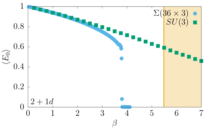
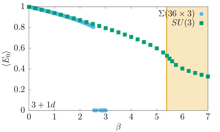
Figure 1: Euclidean calculations of lattice energy density $\langle E_{0}\rangle$ of $\Sigma(36\times 3)$ as measured by the expectation value of the plaquette as a function of Wilson coupling $\beta$ on $8^{d}$ lattices for (top) $(2+1)$-dimensions (bottom) $(3+1)$-dimensions. The shaded region indicates $\beta\geq\beta_{s}$.

This paper is organized as follows. In Sec. II, the group theory needed for $\Sigma(36\times 3)$ are summarized and the digitization scheme is presented. Sec. IV demonstrates the quantum circuits for the four primitive gates required for implementing the group operations: the inversion gate, the multiplication gate, the trace gate, and the Fourier transform gate. Using these gates, Sec. V presents a resource estimates for simulating $3+1d$ $SU(2)$. We conclude and discuss future work in Sec. VI.

II Properties of $\Sigma(36\times 3)$

$\Sigma(36\times 3)$ is a discrete subgroup of SU(3) with 108 elements. The group elements, $g$, of $\Sigma(36\times 3)$ can be written in the following ordered product or otherwise known as strong generating set. That is, all the group elements, $g$, can be enumerated as a product of left or right transversals such that

$$g=\omega^{p}C^{q}E^{r}V^{2s+t},$$ (1)

where $0\leq p,~{}q,~{}r\leq 2$ and $0\leq s,~{}t\leq 1$. This indicates that either 8 qubits (2 each for $p$ , $q$, and $r$, and one each for $s$ and $t$) or 3 qutrits ($p$, $q$, and $r$) and 2 qubits ($s$ and $t$) will be required to store the group register. Because the indices $p,~{}q,$ and $r$ take on values between 0 and 2, there exists an ambiguity in mapping the three-level states to a pair of two-level systems. We use the mapping $|0\rangle_{3}=|00\rangle_{2}$, $|1\rangle_{3}=|01\rangle_{2}$, and $|2\rangle=|10\rangle_{2}$ with the $|11\rangle_{2}$ state being forbidden. Throughout this work, we will use $|\rangle_{3}$ to denote a three-level state and $|\rangle_{2}$ to denote a two-level state when there is the possibility of ambiguity. In this way, the index $p$ is decomposed in binary as $p=p_{0}+2p_{1}$ and encoded as the state $|p\rangle_{3}=|p_{1}p_{0}\rangle_{2}$. This process is done similarly for $q$ and $r$.

The strong generating set shown in Eq. 1 explicitly builds the presentation of the group from subgroups. In this way primitive gates for smaller discrete groups can be used as building blocks to construct efficient primitive gates of larger groups [102, 100, 101]. In the case of $\Sigma(36\times 3)$, the subgroups of interest are as follows: $\omega^{p}$ generates the subgroup $\mathbb{Z}_{3}$; $\omega^{p}C^{q}$ generates the subgroup $\mathbb{Z}_{3}\times\mathbb{Z}_{3}$; $\omega^{p}C^{q}E^{r}$ generates the subgroup $\Delta(27)$; $\omega^{p}C^{q}E^{r}V^{2s}$ generates $\Delta(54)$. Detailed information regarding these subgroups can be found in Ref. [103].

It is useful to have the irreducible representations, irreps, of $\Sigma(36\times 3)$ for deriving a quantum Fourier transformation (see Sec. IV). This group has 14 irreducible representations (irreps). There are four one-dimensional (1d) irreps, eight three-dimensional irreps (3d), and two four-dimensional (4d) irreps. The 1d irreps are:

$$\rho^{(1)}_{a}(g)=i^{a(2s+t)},~{}0\leq a\leq 3.$$ (2)

The eight 3d irreps can be written as

$$\rho^{(3)}_{a,b}(g)=(-1)^{abt}\omega^{(1+b)p}C^{(1+b)q}E^{r}(i^{a}V)^{2s+(-1)^{b}t},$$ (3)

where $0\leq a\leq 3$ and $0\leq b\leq 1$ and the matrices $\omega$, $C$, $E$, and $V$ are given by

$$\omega=e^{2\pi i/3} ,~{}C=\text{Diag}(1,\omega,\omega^{2}),$$

$$~{}E=\begin{pmatrix}0&1&0\\ 0&0&1\\ 1&0&0\end{pmatrix} \text{, and}~{}V=\frac{1}{\sqrt{3}i}\begin{pmatrix}1&1&1\\ 1&\omega&\omega^{2}\\ 1&\omega^{2}&\omega\end{pmatrix}.$$ (4)

The irrep $\rho_{0,0}^{(3)}$ corresponds to the faithful irrep that resembles the fundamental irrep of $SU(3)$. The 4d irreps are given by Eq. (1) with

$$\begin{split}\rho^{(4)}_{b}(\omega)=&\mathbb{1},~{}~{}\rho^{(4)}_{b}(C)=\text{Diag}(\omega^{b},\omega,\omega^{2b},\omega^{2}),\\ \rho^{(4)}_{b}(E)=&\text{Diag}(\omega,\omega^{2b},\omega^{2},\omega^{b}),\\ \rho^{(4)}_{b}(V)=&\begin{pmatrix}0&1&0&0\\ 0&0&1&0\\ 0&0&0&1\\ 1&0&0&0\\ \end{pmatrix}.\end{split}$$ (5)

In addition for conciseness we provide the character table from Ref [103] in Tab. 2, which will be useful in constructing the trace gate.

As we proceed with constructing primitive gates (see Sec. IV),the following “reordering” relations are useful:

$$EC= \omega CE,~{}VC=EV,~{}\text{and}~{}VE=C^{2}V.$$ (6)

One can extend the relations above to derive the generalized reordering relations:

$$V^{2s+t}C^{q}= C^{(1+s)q(1-t)}E^{t(1+s)q}V^{2s+t},$$

$$E^{r}C^{q}= \omega^{rq}C^{q}E^{r},$$

$$V^{2s+t}E^{r}= C^{t(s+1)(3-r)}E^{(1-t)r(1+s)}V^{2s+t}.$$ (7)

Table 2: Character table of $\Sigma(36\times 3)$ with $\omega=e^{2\pi i/3}$ [103].

Size	1	1	1	12	12	9	9	9	9	9	9	9	9	9
Ord.	1	3	3	3	3	2	6	6	4	12	12	4	12	12
$\mathbf{1}^{(0)}$	$1$	$1$	$1$	$1$	$1$	$1$	$1$	$1$	$1$	$1$	$1$	$1$	$1$	$1$
$\mathbf{1}^{(1)}$	$1$	$1$	$1$	$1$	$1$	$\text{-}1$	$\text{-}1$	$\text{-}1$	$i$	$i$	$i$	$\text{-}i$	$\text{-}i$	$\text{-}i$
$\mathbf{1}^{(2)}$	$1$	$1$	$1$	$1$	$1$	$1$	$1$	$1$	$\text{-}1$	$\text{-}1$	$\text{-}1$	$\text{-}1$	$\text{-}1$	$\text{-}1$
$\mathbf{1}^{(3)}$	$1$	$1$	$1$	$1$	$1$	$\text{-}1$	$\text{-}1$	$\text{-}1$	$\text{-}i$	$\text{-}i$	$\text{-}i$	$i$	$i$	$i$
$\mathbf{3}^{(0)}$	$3$	$3\omega$	$3\omega^{2}$	$0$	$0$	$\text{-}1$	$\text{-}\omega$	$\text{-}\omega^{2}$	$1$	$\omega$	$\omega^{2}$	$1$	$\omega$	$\omega^{2}$
$\mathbf{3}^{(1)}$	$3$	$3\omega$	$3\omega^{2}$	$0$	$0$	$1$	$\omega$	$\omega^{2}$	$i$	$i\omega$	$i\omega^{2}$	$\text{-}i$	$\text{-}i\omega$	$\text{-}i\omega^{2}$
$\mathbf{3}^{(2)}$	$3$	$3\omega$	$3\omega^{2}$	$0$	$0$	$\text{-}1$	$\text{-}\omega$	$\text{-}\omega^{2}$	$\text{-}1$	$\text{-}\omega$	$\text{-}\omega^{2}$	$\text{-}1$	$\text{-}\omega$	$\text{-}\omega^{2}$
$\mathbf{3}^{(3)}$	$3$	$3\omega$	$3\omega^{2}$	$0$	$0$	$1$	$\omega$	$\omega^{2}$	$\text{-}i$	$\text{-}i\omega$	$\text{-}i\omega^{2}$	$i$	$i\omega$	$i\omega^{2}$
$\mathbf{3}^{(0)*}$	$3$	$3\omega^{2}$	$3\omega$	$0$	$0$	$\text{-}1$	$\text{-}\omega^{2}$	$\text{-}\omega$	$1$	$\omega^{2}$	$\omega$	$1$	$\omega^{2}$	$\omega$
$\mathbf{3}^{(1)^{*}}$	$3$	$3\omega^{2}$	$3\omega$	$0$	$0$	$1$	$\omega^{2}$	$\omega$	$\text{-}i$	$\text{-}i\omega^{2}$	$\text{-}i\omega$	$i$	$i\omega^{2}$	$i\omega$
$\mathbf{3}^{(2)*}$	$3$	$3\omega^{2}$	$3\omega$	$0$	$0$	$\text{-}1$	$\text{-}\omega^{2}$	$\text{-}\omega$	$\text{-}1$	$\text{-}\omega^{2}$	$\text{-}\omega$	$\text{-}1$	$\text{-}\omega^{2}$	$\text{-}\omega$
$\mathbf{3}^{(3)*}$	$3$	$3\omega^{2}$	$3\omega$	$0$	$0$	$1$	$\omega^{2}$	$\omega$	$i$	$i\omega^{2}$	$i\omega$	$\text{-}i$	$\text{-}i\omega^{2}$	$\text{-}i\omega$
$\mathbf{4}$	$4$	$4$	$4$	$1$	$\text{-}2$	$0$	$0$	$0$	$0$	$0$	$0$	$0$	$0$	$0$
$\mathbf{4}^{\prime}$	$4$	$4$	$4$	$\text{-}2$	$1$	$0$	$0$	$0$	$0$	$0$	$0$	$0$	$0$	$0$

III Basic Gates

In this work, we consider gate sets for both qubit and hybrid qubit-qutrit systems. Our qubit decompositions use the well-known fault tolerant Clifford + T gate set [104]. This choice is informed by the expectation that quantum simulations for lattice gauge theories will ultimately require fault tolerance to achieve quantum advantage [105, 106, 100, 101, 23]. Throughout, we adopt the notation $\oplus_{m}$ to mean addition mod $m$.

For conciseness, we use a larger than necessary gate set which we will later decomposes in terms of T-gate to obtain resource costs. The single qubit gates used are the Pauli rotations, $R_{\alpha}(\theta)=e^{i\theta\alpha/2}$, where $\alpha=X,Y,Z$. We also consider four entangling operations: SWAP, CNOT, and multicontrolled CⁿNOT, and the controlled SWAP (CSWAP). The two-qubit operations can be written as

$$\text{SWAP}~{}|a\rangle|b\rangle=|b\rangle|a\rangle,$$ (8)

$$\text{CNOT}~{}|a\rangle|b\rangle=|a\rangle|b\oplus_{2}a\rangle.$$ (9)

while the multicontrolled generalizations are

$$\text{C}^{n}\text{NOT}~{}\Big{(}\prod_{n}|a_{n}\rangle\Big{)}|b\rangle=\Big{(}\prod_{n}|a_{n}\rangle\Big{)}|b\oplus_{2}\prod_{n}a_{n}\rangle,$$ (10)

$$\text{CSWAP}|a\rangle|b\rangle|c\rangle=|a\rangle|b(1\oplus_{2}a)\oplus_{2}ac\rangle|c(1\oplus_{2}a)\oplus_{2}ba\rangle.$$ (11)

The hybrid encoding uses a more novel set of single, double, and triple qudit gates. The single-qudit two level rotations we consider are denoted by $R^{\alpha}_{b,c}(\theta)$, where $\alpha=\{X,~{}Y,~{}Z\}$ and indicate a Pauli-style rotation between levels $b$ and $c$. The subscripts will be omitted to indicate that the operation is performed on a qubit rather than a qutrit state. Additionally, we account for the primitive two-qudit gate,

$$C^{a}_{b}X^{c}_{d,e}~{},$$ (12)

which corresponds to the CNOT operation controlled on state $b$ of qubit $a$, and targets qubit $c$ with an $X$ operation between the levels $d$ and $e$. We also for conciseness consider the CSum gate:

$$\textsc{CSum}^{a,b}|i\rangle_{a}|j\rangle_{b}=|i\rangle_{a}|i\oplus_{3}j\rangle_{b}.$$ (13)

which is a controlled operation on qubit or qutrit $a$ and targets qutrit $b$. It can be verified that that the CSum (see e.g. Ref. [10, 107]) gate is related to the $C^{a}_{b}X^{c}_{d,e}$ gates by

$$\textsc{CSum}^{a,b} =\left(C^{a}_{1}X^{b}_{0,1}C^{a}_{1}X^{b}_{1,2}\right)\left(C^{a}_{2}X^{b}_{1,2}C^{a}_{2}X^{b}_{0,1}\right).$$ (14)

Finally, we consider multi-controlled versions of both of these gates. The gate $C^{a}_{b}C^{c}_{d}X^{e}_{f,g}$ corresponds to multicontrolled generalization of Eq. (12). The second multiqudit gate is the CCSum which acts as follows

$$\textsc{CCSum}^{a,b,c}|i\rangle_{a}|j\rangle_{b}|k\rangle_{c}=|i\rangle_{a}|j\rangle_{b}|k\oplus_{3}ij\rangle_{c}.$$ (15)

A unique artifact of this choice of quantum gates is that one can decompose multi-controlled gates using the traditional Toffoli staircase decomposition [108, 104, 109].

IV Primitive Gates

We present the primitive gates for a pure gauge theory in the following subsections using the methods developed in previous papers on the binary tetrahedral, $\mathbb{BT}$, and binary octahedral, $\mathbb{BO}$ groups [97, 98, 100]. Using this formulation confers at least two benefits: first, it is possible to design algorithms in a theory- and hardware-agnostic way; second, the circuit optimization is split into smaller, more manageable pieces. This construction begins with defining for a finite group $G$ a $G$-register by identifying each group element with a computational basis state $\ket{g}$. Then, Ref. [97] showed that Hamiltonian time evolution can be performed using a set of primitive gates. These primitive gates are: inversion $\mathfrak{U}_{-1}$, multiplication $\mathfrak{U}_{\times}$, trace $\mathfrak{U}_{\rm Tr}$, and Fourier transform $\mathfrak{U}_{F}$ [97].

The inversion gate, $\mathfrak{U}_{-1}$, is a single register gate that takes a group element to its inverse:

$$\mathfrak{U}_{-1}\ket{g}=\ket{g^{-1}}\text{.}$$ (16)

The group multiplication gate acts on two $G-$registers. It takes the target $G-$register and changes the state to the left-product with the control $G-$register:

$$\mathfrak{U}_{\times}\ket{g}\ket{h}=\ket{g}\ket{gh}.$$ (17)

Left multiplication is sufficient for a minimal set as right multiplication can be implemented using two applications of $\mathfrak{U}_{-1}$ and $\mathfrak{U}_{\times}$, albeit optimal algorithms may take advantage of an explicit construction [96].

The trace of products of group elements appears in lattice Hamiltonians. We can implement these terms by combining $\mathfrak{U}_{\times}$ with a single-register trace gate:

$$\mathfrak{U}_{\operatorname{Tr}}(\theta)\left|g\right>=e^{i\theta\operatorname{Re}\operatorname{Tr}g}\left|g\right>.$$ (18)

The final gate required is the group Fourier transform $\mathfrak{U}_{F}$. The Fourier transform of a finite $G$ is defined as

$$\hat{f}(\rho)=\sqrt{\frac{d_{\rho}}{|G|}}\sum_{g\in G}f(g)\rho(g),$$ (19)

where $|G|$ is the size of the group, $d_{\rho}$ is the dimensionality of the representation $\rho$, and $f$ is a function over $G$. The gate that performs this acts on a single $G$-register with some amplitudes $f(g)$ which rotate it into the Fourier basis:

$$\mathfrak{U}_{F}\sum_{g\in G}f(g)\left|g\right>=\sum_{\rho\in\hat{G}}\hat{f}(\rho)_{ij}\left|\rho,i,j\right>.$$ (20)

The second sum is taken over $\rho$, the irreducible representations of $G$; $\hat{f}$ denotes the Fourier transform of $f$. After performing the Fourier transform, the register is denoted as a $\hat{G}$-register to indicate the change of basis. A schematic example of this gate is show in Fig. 2.

While it is possible to pass the matrix constructed in Fig. 2 into a transpiler, more efficient methods for constructing these operators exist [110, 102, 111, 112, 113, 114]. While method varies in their actualization, the underlying spirit is the same as for the discrete quantum Fourier transformation. The principle method involves building the quantum Fourier transformation up through a series of subgroups. In [114], it was shown that instead of the exponential $\mathcal{O}(4^{n})$ scaling for traditional transpilation, the quantum Fourier transform scales like $\mathcal{O}(\text{polylog}(|2^{n}|))$, where polylog indicates a polynomial of logarithms.

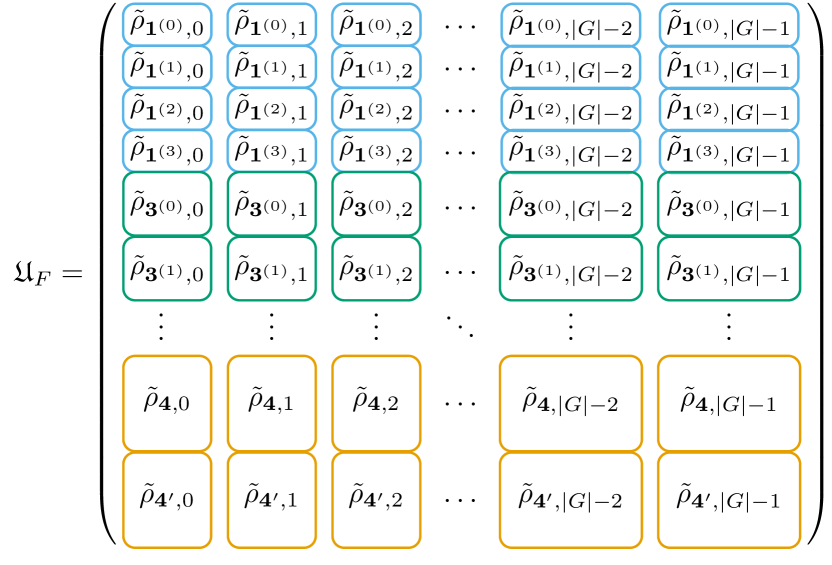
Figure 2: Construction of $\mathfrak{U}_{F}$ from Eq. (19) using column vectors $\tilde{\rho}_{i,j}=\sqrt{d_{\rho}/|G|}\rho_{i,j}$ where $\rho_{i,j}=\rho_{i}(g_{j})$.

In the rest of this paper, we will construct each of these primitive gates, and evaluate the overall cost. For each gate, we will start with a pure qubit system. Then, we will consider a register with three qutrits and two qubits as suggested by the group presentation in Eq. 1.

IV.1 Inversion Gate

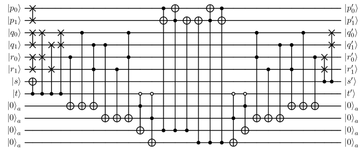
Figure 3: T-gate optimized version of $\mathfrak{U}_{-1}$ for $\Sigma(36\times 3)$. The letter indicates the generator and subscript indicates the qubit in the generator register. This implementation requires 119 T-gates and 4 ancilla.

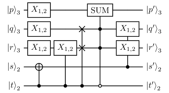
Figure 4: $\mathfrak{U}_{-1}$, for $\Sigma(36\times 3)$ using qutrit-qubit encoding.

For the construction of $\mathfrak{U}_{-1}$, we first write the inverse of the group element $g$ as

$$g^{-1}=\omega^{2p}V^{t+2t}V^{2s}E^{2r}C^{2q}=\omega^{p^{\prime}}C^{q^{\prime}}E^{r^{\prime}}V^{2s^{\prime}+t^{\prime}}.$$ (21)

where the permutations rules are found to be

$$p^{\prime}= 2p\oplus_{3}qr\oplus_{3}2qrt,$$

$$q^{\prime}= 2(q\oplus_{3}qs\oplus_{3}2qt\oplus_{3}rt\oplus_{3}2qst\oplus_{3}rst),$$

$$r^{\prime}= 2(r\oplus_{3}rs\oplus_{3}2qt\oplus_{3}2rt\oplus_{3}2qst\oplus_{3}2rst),$$

$$s^{\prime}= s\oplus_{2}t,$$

$$t^{\prime}= t.$$ (22)

A detailed derivation of the permutation rules and the associated $\mathfrak{U}_{-1}$ is found in App. A along with two other forms of $\mathfrak{U}_{-1}$ which use fewer ancilla. The idealized qubit circuit is shown in Fig. 3 and requires 119 T-gates and 4 clean ancilla. The qubit-qutrit hybrid encoding $\mathfrak{U}_{-1}$ is found in Fig. 4.

IV.2 Multiplication Gate

The multiplication gate $\mathfrak{U}_{\times}$ takes two $G$-registers storing two group elements $g=\omega^{p}C^{q}E^{r}V^{2s+t}$ and $h=\omega^{p^{\prime}}C^{q^{\prime}}E^{r^{\prime}}V^{2s^{\prime}+t^{\prime}}$ and stores into the second register the group element $gh=\omega^{p^{\prime\prime}}C^{q^{\prime\prime}}E^{r^{\prime\prime}}V^{2s^{\prime\prime}+t^{\prime\prime}}$. Using the reordering relations of Eq. (7) one can derive that

$$p^{\prime\prime}= p\oplus_{3}p^{\prime}\oplus_{3}q^{\prime}r\oplus_{3}q^{\prime}rs\oplus_{3}2q^{\prime}rt\oplus_{3}2q^{\prime}r^{\prime}t$$

$$\oplus_{3}2rr^{\prime}t\oplus_{3}2q^{\prime}rst\oplus_{3}2rr^{\prime}st,$$

$$q^{\prime\prime}= q+q^{\prime}+sq^{\prime}\oplus_{3}2tq^{\prime}\oplus_{3}2stq^{\prime}\oplus_{3}2tr^{\prime}\oplus_{3}2str^{\prime},$$

$$r^{\prime\prime}= r\oplus_{3}tq^{\prime}\oplus_{3}stq^{\prime}\oplus_{3}r^{\prime}\oplus_{3}sr^{\prime}\oplus_{3}2tr^{\prime}\oplus_{3}2str^{\prime},$$

$$s^{\prime\prime}= (s\oplus_{2}s^{\prime}\oplus_{2}tt^{\prime}),$$

$$t^{\prime\prime}= (t\oplus_{2}t^{\prime}).$$ (23)

These rules are rather clunky and in order to write a systematic multiplication gate we decompose $\mathfrak{U}_{\times}$ into the following product,

$$\mathfrak{U}_{\times}=\mathfrak{U}_{\times,\omega}\mathfrak{U}_{\times,C}\mathfrak{U}_{\times,E}\mathfrak{U}_{\times,V^{2}}\mathfrak{U}_{\times,V},$$ (24)

where $\mathfrak{U}_{\times,O}$ indicate multiplying the state of the $O$ generator register from the $g_{1}$ register onto the $g_{2}$ register. The breakdown of using this method and the product rules from Eq. (IV.2) yields the circuits composed in Fig. 5 and 6 for the two encodings.

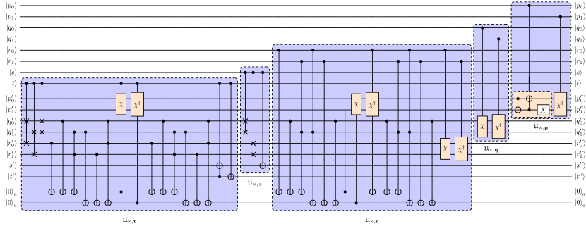
Figure 5: Qubit implementation of $\mathfrak{U}_{\times}$ using the permutation gate $\chi$ and its inverse (both shaded orange) using 2 ancilla and has cost of 308 T-gates.

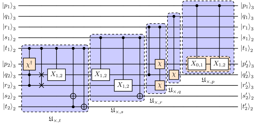
Figure 6: Qutrit+Qubit implementation of $\mathfrak{U}_{\times}$ using the permutation gate $\chi=X^{(0,1)}X^{(1,2)}$ and its inverse (both shaded orange).

IV.3 Trace Gate

There are two principle methods one could derive $\mathfrak{U}_{Tr}$. One method is to define a Hamiltonian of the form:

$$\hat{H}_{Tr}=\sum_{g}Tr(g)|g\rangle\langle g|.$$ (25)

Then, the trace operator can be written as $\mathfrak{U}_{Tr}\left(\theta\right)=\exp{\left(-\mathrm{i}\,\theta\,H_{{\rm Tr}}\right)}$. To obtain the matrix form of $\hat{H}_{Tr}$, one may fix a basis $\left\{|g_{1}\rangle,{...},|g_{|G|}\rangle\right\}$ where $|G|=108$ is the order of the group. In this basis, $\hat{H}_{Tr}$ is diagonal, and each diagonal entry is given by $H_{i,i}=Tr(g_{i})$.

To obtain a quantum circuit realizing $\mathfrak{U}_{{\rm Tr}}$, we use the tree-traversal algorithm developed in [115] which was shown to yield an exact circuit with asymptotically optimal CNOT gates count. The circuit obtained has 130 CNOT gates and 111 $R_{z}$ gates. Additional methods are also found in Ref. [116]. A second method for deriving this gate involves mapping group elements to their respective trace classes. $\Sigma(36\times 3)$ has 14 conjugacy classes that map to 10 different trace classes. If we only require the real part of the trace then this grouping reduces the 10 trace classes to 7 trace classes. The seven valid traces are ${\rm ReTr}(g)=\{3,-\frac{3}{2},0,\pm 1,\pm\frac{1}{2}\}$, which we can be labelled using three bits $\left(v_{0},v_{1},v_{2}\right)$ as shown in Table 3.

$\operatorname{Re}\operatorname{Tr}(g)$	$-3$	$-\frac{3}{2}$	$-1$	$-\frac{1}{2}$	0	1	$\frac{1}{2}$
$v_{0}$	0	1	0	1	0	0	1
$v_{1}$	0	0	1	0	1	0	1
$v_{2}$	0	0	1	1	0	1	1

Table 3: Map $(p,q,r,s,t)\mapsto(v_{0},v_{1},v_{2})$ via ${\rm{Re}Tr}(g)$.

This map can be represented as three boolean functions, one for each of the variables $v_{0}$, $v_{1}$ and $v_{2}$. For quantum computation, it is convenient to write boolean functions in the so-called exclusive-or sum of products (ESOP) form [117, 118]. Then, the function can be mapped to a quantum circuit in a straightforward manner since each term in the ESOPs corresponds to a Toffoli gate. For each function, we start with their minterm forms [119]. Then, we use the exorcism algorithm to find a simpler ESOP expression for each of the three functions. After factorizations, we show the final expressions in Eq. 26.

$$v_{0}= \bar{p}_{0}\left[1\oplus_{2}\bar{t}\left(q_{0}r_{1}\oplus_{2}q_{1}r_{0}\right)\oplus_{2}\bar{s}\left(\bar{q}_{0}\bar{r}_{0}\oplus_{2}\bar{q}_{1}\bar{r}_{1}\right)\right]$$

$$\oplus_{2}\bar{p}_{1}\left[t\oplus_{2}s\left(\bar{q}_{1}\bar{r}_{0}\oplus_{2}\bar{q}_{0}\bar{r}_{1}\right)\right]$$

$$\oplus_{2}\bar{p}_{1}\bar{t}(q_{0}\oplus_{2}\bar{q}_{1})(r_{0}\oplus_{2}\bar{r}_{1}),$$

$$v_{1}= \bar{t}\oplus_{2}(q_{0}\oplus_{2}\bar{q}_{1})(r_{0}\oplus_{2}\bar{r}_{1})\bar{s}\bar{t},$$

$$v_{2}= s\oplus\bar{s}t.$$ (26)

$\mathfrak{U}_{Tr}$ can be decomposed as $\mathfrak{U}_{Tr}(\theta)=V\,\mathfrak{U}^{\prime}_{Tr}(\theta)V^{\dagger}$ where $V$ is a unitary operator realizing the map $\left(p,q,r,s,t\right)\mapsto\left(v_{0},v_{1},v_{2}\right)$. This yields $\mathfrak{U}^{\prime}_{Tr}(\theta)\equiv e^{\mathrm{i}\theta H^{\prime}}$, where

$$H^{\prime}= \frac{3}{16}III+\frac{3}{16}IIZ+\frac{3}{16}IZI+\frac{5}{16}IZZ$$

$$+\frac{1}{16}ZII+\frac{9}{16}ZIZ+\frac{9}{16}ZZI+\frac{15}{16}ZZZ.$$ (27)

Figure 7 shows the quantum circuit of the operator $V$ realizing the map $\left(p,q,r,s,t\right)\mapsto\left(v_{0},v_{1},v_{2}\right)$. Finally, the circuit of $\mathfrak{U_{Tr}}^{\prime}(\theta)$ is shown in Figure 8.

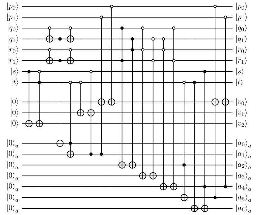
Figure 7: Quantum Circuit of the map $\left(p,q,r,s,t\right)\mapsto\left(v_{0},v_{1},v_{2}\right)$ from the group to the seven real trace classes ${\rm ReTr(g)}=\{3,-1.5,0,\pm 1,\pm 0.5\}$. This requires 15 Toffoli gates and thus 105 T gates

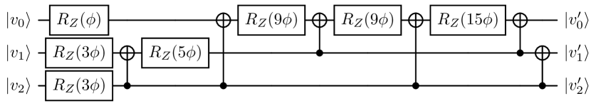
Figure 8: Quantum circuit of the operator $\mathfrak{U}^{\prime}_{Tr}(\theta)$ where we have set $\phi\equiv-\frac{\theta}{8}$.

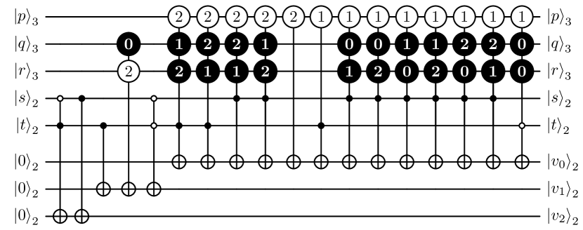
Figure 9: Quantum Circuit of the map $\left(p,q,r,s,t\right)\mapsto\left(v_{0},v_{1},v_{2}\right)$ from the group to the seven real trace classes ${\rm ReTr(g)}=\{3,-1.5,0,\pm 1,\pm 0.5\}$ for qutrit+qubit. In analogy to the closed and open circle notation for control qubits, the black and white qutrit controls represent controlled-on or controlled-on-others e.g. a white 1 is a control qutrit which applies a gate if in the state $\ket{0}$ or $\ket{2}$.

IV.4 Fourier Transform Gate

The standard $n$-qubit quantum Fourier transform (QFT) [120] corresponds to the quantum version of the fast Fourier transform of $\mathbb{Z}_{2^{n}}$. Quantum Fourier transforms, $\mathfrak{U}_{QFT}$, over some nonabelian groups are known [111, 112, 102, 114, 98]. However, for all the crystal-like subgroups of interest to high energy physics $\mathfrak{U}_{QFT}$ is currently unknown [121] and there is not a clear algorithmic way to construct $\mathfrak{U}_{QFT}$ in general. Therefore, we instead construct a suboptimal $\mathfrak{U}_{F}$ from Eq. (19) using the irreps of Sec. II. The structure of $\mathfrak{U}_{F}$ is ordered as follows. The columns index $|g\rangle$ from $\ket{0}$ to $\ket{256}$ according to Eq. (1). We then index the irreducible representation $\rho_{i}$ ordered sequentially from $i=1$ to $i=14$.

Since $\Sigma(36\times 3)$ has 108 elements, on a qubit device $\mathfrak{U}_{F}$ must be embedded into a larger $2^{8}\times 2^{8}=256\times 256$ matrix. While the matrix This matrix was then passed to the Qiskit v0.43.1 transpiler, and an optimized version of $\mathfrak{U}_{F}$ needed 30956 CNOTs, 2666 $R_{X}$, 32806 $R_{Y}$, and 55234 $R_{Z}$ gates; the Fourier gate is the most expensive qubit primitive. As will be discussed in Sec. V, $\mathfrak{U}_{F}$ dominates the total simulation costs and future work should be devoted to finding a $\Sigma(36\times 3)$ $\mathfrak{U}_{QFT}$ .

For the hybrid qubit-qutrit implementation, $\mathfrak{U}_{F}$ is of dimensions $108\times 108$. To obtain a quantum circuit, we built a qubit-qutrit compiler, see Ref. [122]. The outline of the compilation is discussed in Appendix B. The compiler uses the gates discussed in Sec. III, and Table 4 shows its resulting gates count.

Basic Gate	$\mathcal{U}_{-1}$	$\mathcal{U}_{\times}$	$\mathcal{U}_{Tr}$	$\mathcal{U}_{F}$
$R_{\alpha}$	0	0	7	92,568
$R^{\alpha}_{b,c}$	3	0	0	35,310
CNOT	1	2	9	16,656
C2NOT	0	1	2	0
C3NOT	0	0	0	0
C4NOT	0	0	0	0
$C_{2}X_{b,c}$	2	3	0	67,260
$C_{3}X_{b,c}$	12	20	1	8,988
$C_{3}C_{2}X_{b,c}$	8	12	13	0
$C_{3}C_{3}X_{b,c}$	4	36	45	0

Table 4: Gate cost of primitive gates for $\Sigma(36\times 3)$ for a qutrit-qubit architecture. The costs for $\mathcal{U}_{F}$ were obtained with the hybrid compiler described in Appendix B. $C_{d}X_{b,c}$ refers to an $X$ rotation between states $b,c$ of a qutrit controlled by a qudit with $d$ levels

V Resource Costs

The relatively deep circuits presented above strongly suggest that simulating $\Sigma(36\times 3)$ will require error correction. The preclusion of universal transversal sets of gates stated in the Eastin-Knill theorem [123] requires compromises be made. In most error correcting codes, the Clifford gates are designed to be transversal [104, 124, 125, 126, 127]. This leaves the nontransversal T gate as the dominant cost of fault-tolerant algorithms [104, 128]. Beyond these standard codes, novel universal sets exist with transversal $\mathbb{BT},\mathbb{BO},\mathbb{BI}$ and He(3) gates [129, 130, 131, 132, 133] which warrant exploration for use in lattice gauge theory.

Table 5: Number of physical T gates and clean ancilla required to implement logical gates for (top) basic gates taken from [104] (bottom) primitive gates for $\Sigma(36\times 3)$.

Gate	T gates	Clean ancilla
C2NOT	7	0
C3NOT	21	1
C4NOT	35	2
CSWAP	7	0
$R_{Z}$	1.15 $\log_{2}(1/\epsilon)$	0
$\mathcal{U}_{-1}$	119	4
$\mathcal{U}_{\times}$	308	2
$\mathcal{U}_{Tr}$	$210+8.05\log_{2}(1/\epsilon)$	7
$\mathcal{U}_{F}$	$185897.5\log_{2}(1/\epsilon)$	0

For this work we will consider the following decompositions of gates into T gates for our resource estimates. First, while the CNOT is transversal, the Toffoli gate decomposes into six CNOTs and seven T gates [104]. With this, one can construct any CⁿNOT gates using $2\lceil\log_{2}{n}\rceil-1$ Toffoli gates and $n-2$ dirty ancilla qubits which can be reused later [108, 104, 109]. For the $R_{Z}$ gates, we use the repeat-until-success method of [134] which finds these gates can be approximated to precision $\epsilon$ with on average $1.15\log_{2}(1/\epsilon))$ T gates (and at worst $-9+4\log_{2}(1/\epsilon)$ [135]). For $R_{Y}$ and $R_{X}$, one can construct them with at most 3 $R_{Z}$. Putting all together, we can construct gate estimates for $\Sigma(36\times 3)$ (See Tab. 5).

Table 6: Number of primitive gates per link per $\delta t$ neglecting boundary effects as a function of $d$ for $H_{KS}$ and $H_{I}$.

Gate	$\mathfrak{U}_{F}$	$\mathfrak{U}_{\rm Tr}$	$\mathfrak{U}_{-1}$	$\mathfrak{U}_{\times}$
$e^{-i\delta H_{KS}}$	2	$\frac{1}{2}(d-1)$	$3(d-1)$	$6(d-1)$
$e^{-i\delta H_{I}}$	4	$\frac{3}{2}(d-1)$	$2+11(d-1)$	$4+26(d-1)$

While the results in Tab. 5 are nearly optimal for the $\mathfrak{U}_{\operatorname{Tr}}$, $\mathfrak{U}_{\times}$, and $\mathfrak{U}_{-1}$, the result for $\mathfrak{U}_{F}$ is not. In Ref. [110] the authors show explicit demonstrations of an efficient decomposition of the nonabelian quantum Fourier transform $\mathfrak{U}_{QFT}$ using the methods of [102] for certain $SU(2)$ and $SU(3)$ subgroups. Since it is expected that the gate cost for Fourier transforms should scale as a polynomial of logarithms of the group size [114], one can perform a fit from the results in Ref. [110] to obtain an order of magnitude estimate for $\mathfrak{U}_{QFT}$ of $147+75\rm{log}_{2}(1/\epsilon)$ – a factor of $\sim 2000$ smaller than our $\mathfrak{U}_{F}$.

Clearly, the cost of simulating $\Sigma(36\times 3)$ depends on $\epsilon$. To optimize the cost, the synthesis error from finite $\epsilon$ should be balanced with other sources of error in the quantum simulation like Trotter error, discretization error, and finite volume error. These other sources of error are highly problem-dependent, but here we will follow prior works [136, 42, 137] and take a fiducial $\epsilon=10^{-8}$.

Primitive gate costs for implementing $H_{KS}$ [138] and $H_{I}$ [96], per link per Trotter step $\delta t$ are shown in Tab. 6. Using this result, we can determine the total T gate count $N^{H}_{T}=C^{H}_{T}\times dL^{d}N_{t}$ for a $d$ spatial lattice simulated for a time $t=N_{t}\delta t$. We find that for $H_{KS}$

$$C^{KS}_{T}=2310(d-1)+(371791+4.025d)\log_{2}\frac{1}{\epsilon}.$$ (28)

With this, the total synthesis error $\epsilon_{T}$ can be estimated as the sum of $\epsilon$ from each $R_{Z}$. In the case of $H_{KS}$ this is

$$\epsilon_{T}=\frac{1}{2}(646593+7d)dL^{d}N_{t}\times\epsilon.$$ (29)

If one looks to reduce lattice spacing errors for a fixed number of qubits, one can use $H_{I}$ which would require

$$C^{I}_{T}=9632d-8192+(743578+12.075d)\log_{2}\frac{1}{\epsilon},$$ (30)

where the total synthesis error is

$$\epsilon_{T}=\frac{1}{2}(1293179+21d)dL^{d}N_{t}\times\epsilon.$$ (31)

Following [139, 136, 100], we will make resource estimates based on our primitive gates for the calculation of the shear viscosity $\eta$ on a $L^{3}=10^{3}$ lattice evolved for $N_{t}=50$, and total synthesis error of $\epsilon_{T}=10^{-8}$. Considering only the time evolution and neglecting state preparation (which can be substantial [140, 141, 142, 143, 144, 145, 146, 147, 75, 148, 149, 150, 151, 150, 152, 153, 154]), Kan and Nam estimated $6.5\times 10^{48}$ T gates would be required for an pure-gauge $SU(3)$ simulation of $H_{KS}$. This estimate used a truncated electric-field digitization and considerable fixed-point arithmetic – greatly inflating the T gate cost. Here, using $\Sigma(36\times 3)$ to approximate $SU(3)$ requires $7.0\times 10^{12}$ T gates for $H_{I}$ and $3.5\times 10^{12}$ T gates for $H_{KS}$. The T gate density is roughly 1 per $\Sigma(36\times 3)-$register per clock cycle. Thus $\Sigma(36\times 3)$ reduces the gate costs of [136] by $10^{36}$. Similar to the previous results for discrete groups of SU(2), $\mathfrak{U}_{F}$ dominates the simulations – being over 99% of the computation regardless of Hamiltonian. However [110] shows that the Fourier transformation for $\mathbb{BT}$ and $\mathbb{BO}$ can be brought down. Using the estimate for $\Sigma(36\times 3)$, the Fourier gate contribution is reduced to only 51% of the simulation with a reduced total T gate count of $5.7\times 10^{9}$ for $H_{I}$ with $L=10$ .

VI Outlook

This article provided a construction of primitive gates necessary to simulate a pure SU(3) gauge theory via a discrete subgroup $\Sigma(36\times 3)$. In addition, we have also estimated the T-gate cost incurred to compute the shear viscosity using the $\Sigma(36\times 3)$ group. Notably, we found that our construction improves the T-gate cost upon that of Ref. [136] by 36 orders of magnitude. This cost reduction comes at the expense of model accuracy.

For both qubit and hybrid qubit-qutrit implementations, $\mathfrak{U}_{F}$ dominates the cost suggesting that further reductions by identifying a $\mathfrak{U}_{QFT}$ for $\Sigma(36\times 3)$. In fact, as demonstrated in Ref. [110], the cost of a $\mathfrak{U}_{QFT}$ versus $\mathfrak{U}_{F}$ can be as large as a factor of $\sim 2000$.

In addition, the much-improved overall cost due to the use of the $\Sigma(36\times 3)$ group supports the need to also study other discrete subgroups of SU(2) and SU(3). To this end, recent studies (e.g. Ref [100, 101]) have already constructed primitive gates for some SU(2) discrete subgroups, the binary tetrahedral and binary octahedral. It remains to develop such gates for other subgroups, for example the larger subgroups of SU(3) such as $\Sigma(72\times 3)$, $\Sigma(216\times 3)$ and $\Sigma(360\times 3)$ as well as the $\mathbb{BI}$ group. The larger groups will reduce discretization errors but at the cost of a longer circuit depth.

Finally, beyond pure gauge, approximating QCD requires incorporating fermion fields [155, 79, 156]. Many methods exist to incorporate staggered and Wilson fermions. It is worth comparing the resource costs for explicit spacetime simulations using staggered versus Wilson fermions not only in terms of T-gates but also spacetime costs using methods such as [157].

Appendix A Derivation of Inversion Gates

The inversion rules from Eq. (IV.1) are written in a three level notation. If one wants to simulate systems using qubits one needs to map these to a qudit basis rules to qubit basis rules. We first begin with the $p^{\prime}$ rule

$$p^{\prime}= 2p\oplus_{3}qr(1-t)$$

$$= 2(p_{0}\oplus_{3}2p_{1})\oplus_{3}(q_{0}\oplus_{3}2q_{1})(r_{0}\oplus_{3}2r_{1})(1-t)$$

$$= 2(p_{0}\oplus_{3}2p_{1})\oplus_{3}(1-t)\big{(}q_{0}r_{0}\oplus_{3}2q_{1}r_{0}$$

$$\oplus_{3}2r_{1}q_{0}\oplus_{3}4q_{1}r_{1}\big{)}.$$

In order to turn this trinary arithmetic into binary arithmetic we need the following transformation axiom:

$$p^{\prime}= p\oplus_{3}1,$$

$$p_{0}^{\prime}= p_{0}\oplus_{2}p_{1}\oplus_{2}1,$$

$$p_{1}^{\prime}= p_{0},$$ (32)

and

$$p^{\prime}= p\oplus_{3}2,$$

$$p_{0}^{\prime}= p_{1},$$

$$p_{1}^{\prime}= p_{1}\oplus_{2}p_{0}\oplus_{2}1.$$ (33)

Using this set of transformation rules we find

$$p_{0}^{\prime}= p_{1}\oplus_{2}(1\oplus_{2}t)\big{(}(1\oplus_{2}p_{0})(q_{0}r_{0}\oplus_{2}q_{1}r_{1})$$

$$\oplus_{2}p_{0}(q_{1}r_{0}\oplus_{2}r_{1}q_{0})\big{)},$$

$$p_{1}^{\prime}= p_{0}\oplus_{2}(1\oplus_{2}t)\big{(}(1\oplus_{2}p_{1})(q_{1}r_{0}\oplus_{2}q_{0}r_{1})$$

$$\oplus_{2}p_{1}(q_{0}r_{0}\oplus_{2}q_{1}r_{1})\big{)},$$

$$q_{0}^{\prime}= q_{1}(1\oplus_{2}s)(1\oplus_{2}t)\oplus_{2}q_{0}s(1\oplus_{2}t)$$

$$\oplus_{2}r_{1}(1\oplus_{2}s)t\oplus_{2}r_{0}st,$$

$$q_{1}^{\prime}= q_{0}(1\oplus_{2}s)(1\oplus_{2}t)\oplus_{2}q_{1}s(1\oplus_{2}t)$$

$$\oplus_{2}r_{0}(1\oplus_{2}s)t\oplus r_{1}st,$$

$$r_{0}^{\prime}= r_{1}(1\oplus_{2}s)(1\oplus_{2}t)\oplus_{2}r_{0}s(1\oplus_{2}t)$$

$$\oplus q_{0}t(1\oplus_{2}s)\oplus q_{1}ts,$$

$$r_{1}^{\prime}= r_{0}(1\oplus_{2}s)(1\oplus_{2}t)\oplus_{2}r_{1}s(1\oplus_{2}t)$$

$$\oplus_{2}q_{1}t(1\oplus_{2}s)\oplus_{2}q_{0}ts.$$ (34)

Naively translating these rules as written yields the circuit provided in Fig. 10. However the resource cost of 420 T-gates can be optimized significantly. By clever use of ancillae one could reduce the T-gate costs down to 203 T-gates using the circuit provided in Fig. 11.

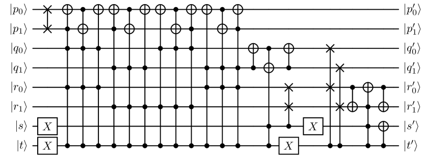
Figure 10: $\mathfrak{U}_{-1}$ for $\Sigma(108)$ which requires 420-T gates.

Instead of writing a circuit for the circuit for the whole inversion ruleset of Eq. (IV.1), one instead could use commutation rules to reduce the T-gate costs even further. This construction allows the inversion operation to be decomposed into a product of smaller operations:

$$\mathfrak{U}_{-1}=\mathfrak{U}_{-1}^{C}\mathfrak{U}_{-1}^{E}\mathfrak{U}_{-1}^{V^{2}}\mathfrak{U}_{-1}^{V}\mathfrak{U}_{-1}^{l}.$$ (35)

$\mathfrak{U}_{-1}^{l}$ takes each local generator to its inverse:

$$t\rightarrow t$$

$$s\rightarrow s\oplus_{2}t$$

$$r\rightarrow 2r$$

$$q\rightarrow 2q$$

$$p\rightarrow 2p.$$

The operation $\mathfrak{U}_{-1}^{V}$ involves propagating through the operator $V^{t}$ until it is the right most element. This yields the transformations:

$$s\rightarrow s$$

$$r\rightarrow r(1-t)\oplus_{3}qt$$

$$q\rightarrow 2rt\oplus_{3}q(t-1)$$

$$p\rightarrow p\oplus_{3}rq(1-t).$$

The generators $C$ and $E$ are normal ordered at this point. The operation $\mathfrak{U}_{-1}^{V^{2}}$ has the following transformation rule

$$r\rightarrow 2rs\oplus_{3}r(1-s)$$

$$q\rightarrow 2qs\oplus_{3}q(1-s)$$

$$p\rightarrow p.$$

At this point the transformation rules for $C,~{}E,$ and $\omega$ are trivial. After all these suboperations are constructed we end up with the inversion operation from the main text provided in Fig. 3 and Fig. 4.

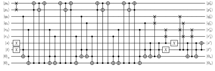
Figure 11: A more $T$-gate optimized version of $\mathfrak{U}_{-1}$ for $\Sigma(108)$ which requires requires 203-T gates and 2 ancilla.

Appendix B Qubit-Qutrit Compiler

This section details the compilation method, and the full codes can be found in Ref. [122]. The overarching approach of this compiler is to generalize the qubit Quantum Shannon Decomposition (QSD) [158, 159] to apply to a register with qubits and qutrits. We will consider a unitary operator $U$ acting on $n_{1}$ qubits and $n_{2}$ qutrits; that is $U$ is of dimension $N\times N$ where $N=2^{n_{1}}\times 3^{n_{2}}$.

First, let’s organize the qudits as $q_{1},q_{2},{...},q_{n_{1}+n_{2}}$. We will say that the left-most qudit is the top qudit. The compiler iteratively performs the qubit QSD if the top qudit is a qubit, and otherwise performs our realization of the qutrit QSD. The process eventually terminates when we reach the bottom qudit, in which case, we use either a single-qubit gate decomposition or a single-qutrit gate decomposition depending on whether the bottom qudit is qubit of qutrit. For the single qubit gate, we use the Euler angle parametrization $ZYZ$ and for the single qutrit gate, we use the decomposition given in Ref. [107].

It is convenient to start with the qubit QSD case. In this case, a Cosine-Sine decomposition (CSD) (see e.g. Refs. [160, 161, 162]) is first performed, resulting in

$$U=(V_{1}\oplus V_{2})\begin{pmatrix}C&-S\\ S&C\\ \end{pmatrix}(W_{1}\oplus W_{2}),$$ (36)

where $V_{1,2}$, $W_{1,2}$ are unitaries with dimension $N/2$. $C$ and $S$ are diagonal matrices e.g $C=\rm{diag}\left(\cos\theta_{1},{...},\cos\theta_{N/2}\right)$ and similarly for $S$.

Following [158], the next step is to decompose the two block-diagonal unitary matrices:

$$\left(V_{1}\oplus V_{2}\right) =(\mathbb{1}\otimes M)(D\oplus D^{\dagger})(\mathbb{1}\otimes N).$$ (37)

where $M$ and $N$ are unitaries acting only on $n_{1}-1$ qubits and $n_{2}$ qutrits, and $D$ is a diagonal unitary of dimension $N/2$. Thus, the compilation problem is reduced to decomposing the unitaries $D\oplus D^{\dagger}$ and the $CS$ into simple gates. The $D\oplus D^{\dagger}$ can be implemented as a uniformly controlled rotations on the top qudit (see e.g. Ref. [158]). The $CS$ matrix on the other hand, is related to $D\oplus D^{\dagger}$ by the rotation gate $R_{x}(\pi/2)$ on the top qubit. This concludes the case the top qudit is a qubit.

In the case that the top qudit is qutrit, we need to find a qutrit realization of the procedure above. The starting point is to perform two CSD as in e.g. Ref. [163]. This decomposition reads as

$$U=\left(V_{1}\oplus V_{2}\oplus V_{3}\right) \left(\mathbb{1}\oplus D\oplus D^{\dagger}\right)\left(W_{1}\oplus W_{2}\oplus W_{3}\right)\begin{pmatrix}C&&-S\\ &\mathbb{1}&\\ S&&C\end{pmatrix}\left(V^{\prime}_{1}\oplus V^{\prime}_{2}\oplus V^{\prime}_{3}\right)\left(\mathbb{1}\oplus D^{\prime}\oplus D^{\prime\dagger}\right)\left(W^{\prime}_{1}\oplus W^{\prime}_{2}\oplus W^{\prime}_{3}\right),$$ (38)

where each block is a unitary of dimension $N/3$. The blocks $C$, $S$ $D$ and $D^{\prime}$ are defined analogously to the qubit case.

The rest is to decompose the remaining block diagonal unitaries. By performing the decomposition in Ref. [158] twice, we obtain the relation

$$V_{1}\oplus V_{2}\oplus V_{3}=\left(\mathbb{1}_{3\times 3}\otimes M\right)\left(D\oplus D\oplus D^{\dagger}\right)\left(\mathbb{1}_{3\times 3}\otimes N\right) \left(D^{\prime}\oplus D^{\prime\dagger}\oplus\mathbb{1}\right)\left(\mathbb{1}_{3\times 3}\otimes M^{\prime}\right)\left(D^{\prime\prime}\oplus D^{\prime\prime}\oplus D^{\prime\prime\dagger}\right)\left(\mathbb{1}_{3\times 3}\otimes N^{\prime}\right).$$ (39)

The unitaries $\mathbb{1}\oplus D\oplus D^{\dagger}$, $D\oplus D^{\dagger}\oplus\mathbb{1}$, $D\oplus D\oplus D^{\dagger}$ and $CS$ are uniformly controlled rotations. We can focus on the diagonal blocks because as in the qubit case, the $CS$ matrix can be diagonalized with an appropriate $R^{i,j}_{x}(\pi/2)$ on the top qutrit. Ref. [164] outlines the decomposition of qutrits uniformly controlled rotations in terms of single- and two-qutrit gates. A generalization can be obtained simply by limiting a $C^{a}_{b}X^{c}_{i,j}$ gate to $C^{a}_{1}X^{c}_{i,j}$ when the control qudit is a qubit.

For $n=2$ qubits, there exists optimal compilation algorithms (see e.g. Ref. [165]). Therefore, when the bottom two qudits are both qubits, we stop the decomposition and use Qiskit transpiler to obtain a quantum circuit.

References

- Aarts [2016] G. Aarts, Introductory lectures on lattice qcd at nonzero baryon number, Journal of Physics: Conference Series 706, 022004 (2016).
- Philipsen [2007] O. Philipsen, Lattice qcd at finite temperature and density, The European Physical Journal Special Topics 152, 29 (2007).
- de Forcrand [2010] P. de Forcrand, Simulating qcd at finite density (2010), arXiv:1005.0539 [hep-lat] .
- Muroya et al. [2003] S. Muroya, A. Nakamura, C. Nonaka, and T. Takaishi, Lattice QCD at Finite Density: An Introductory Review, Progress of Theoretical Physics 110, 615 (2003).
- Gattringer and Langfeld [2016] C. Gattringer and K. Langfeld, Approaches to the sign problem in lattice field theory, Int. J. Mod. Phys. A 31, 1643007 (2016), arXiv:1603.09517 [hep-lat] .
- Alexandru et al. [2018] A. Alexandru, P. F. Bedaque, H. Lamm, S. Lawrence, and N. C. Warrington, Fermions at Finite Density in 2+1 Dimensions with Sign-Optimized Manifolds, Phys. Rev. Lett. 121, 191602 (2018), arXiv:1808.09799 [hep-lat] .
- Alexandru et al. [2022] A. Alexandru, G. m. c. Başar, P. F. Bedaque, and N. C. Warrington, Complex paths around the sign problem, Rev. Mod. Phys. 94, 015006 (2022).
- Troyer and Wiese [2005] M. Troyer and U.-J. Wiese, Computational complexity and fundamental limitations to fermionic quantum Monte Carlo simulations, Phys. Rev. Lett. 94, 170201 (2005), arXiv:cond-mat/0408370 [cond-mat] .
- Gustafson et al. [2021] E. Gustafson et al., Large scale multi-node simulations of gauge theory quantum circuits using Google Cloud Platform, in IEEE/ACM Second International Workshop on Quantum Computing Software (2021) arXiv:2110.07482 [quant-ph] .
- Gustafson [2021] E. Gustafson, Prospects for Simulating a Qudit Based Model of (1+1)d Scalar QED, Phys. Rev. D 103, 114505 (2021), arXiv:2104.10136 [quant-ph] .
- Popov et al. [2024] P. P. Popov, M. Meth, M. Lewenstein, P. Hauke, M. Ringbauer, E. Zohar, and V. Kasper, Variational quantum simulation of U(1) lattice gauge theories with qudit systems, Phys. Rev. Res. 6, 013202 (2024).
- Kurkcuoglu et al. [2022] D. M. Kurkcuoglu, M. S. Alam, J. A. Job, A. C. Y. Li, A. Macridin, G. N. Perdue, and S. Providence, Quantum simulation of theories in qudit systems (2022), arXiv:2108.13357 [quant-ph] .
- Calajò et al. [2024] G. Calajò, G. Magnifico, C. Edmunds, M. Ringbauer, S. Montangero, and P. Silvi, Digital quantum simulation of a (1+1)D SU(2) lattice gauge theory with ion qudits (2024), arXiv:2402.07987 [quant-ph] .
- González-Cuadra et al. [2022] D. González-Cuadra, T. V. Zache, J. Carrasco, B. Kraus, and P. Zoller, Hardware efficient quantum simulation of non-abelian gauge theories with qudits on Rydberg platforms (2022), arXiv:2203.15541 [quant-ph] .
- Illa et al. [2024a] M. Illa, C. E. P. Robin, and M. J. Savage, Qu8its for quantum simulations of lattice quantum chromodynamics (2024a), arXiv:2403.14537 [quant-ph] .
- Zache et al. [2023a] T. V. Zache, D. González-Cuadra, and P. Zoller, Fermion-qudit quantum processors for simulating lattice gauge theories with matter, Quantum 7, 1140 (2023a).
- Unmuth-Yockey et al. [2018] J. Unmuth-Yockey, J. Zhang, A. Bazavov, Y. Meurice, and S.-W. Tsai, Universal features of the Abelian Polyakov loop in 1+1 dimensions, Phys. Rev. D98, 094511 (2018), arXiv:1807.09186 [hep-lat] .
- Unmuth-Yockey [2019] J. F. Unmuth-Yockey, Gauge-invariant rotor Hamiltonian from dual variables of 3D gauge theory, Phys. Rev. D 99, 074502 (2019), arXiv:1811.05884 [hep-lat] .
- Klco et al. [2020] N. Klco, J. R. Stryker, and M. J. Savage, SU(2) non-Abelian gauge field theory in one dimension on digital quantum computers, Phys. Rev. D 101, 074512 (2020).
- Farrell et al. [2023] R. C. Farrell, M. Illa, A. N. Ciavarella, and M. J. Savage, Scalable Circuits for Preparing Ground States on Digital Quantum Computers: The Schwinger Model Vacuum on 100 Qubits (2023), arXiv:2308.04481 [quant-ph] .
- Farrell et al. [2024] R. C. Farrell, M. Illa, A. N. Ciavarella, and M. J. Savage, Quantum Simulations of Hadron Dynamics in the Schwinger Model using 112 Qubits (2024), arXiv:2401.08044 [quant-ph] .
- Illa et al. [2024b] M. Illa, C. E. P. Robin, and M. J. Savage, Qu8its for Quantum Simulations of Lattice Quantum Chromodynamics (2024b), arXiv:2403.14537 [quant-ph] .
- Ciavarella et al. [2021] A. Ciavarella, N. Klco, and M. J. Savage, A Trailhead for Quantum Simulation of SU(3) Yang-Mills Lattice Gauge Theory in the Local Multiplet Basis (2021), arXiv:2101.10227 [quant-ph] .
- Bazavov et al. [2015] A. Bazavov, Y. Meurice, S.-W. Tsai, J. Unmuth-Yockey, and J. Zhang, Gauge-invariant implementation of the Abelian Higgs model on optical lattices, Phys. Rev. D92, 076003 (2015), arXiv:1503.08354 [hep-lat] .
- Zhang et al. [2018] J. Zhang, J. Unmuth-Yockey, J. Zeiher, A. Bazavov, S. W. Tsai, and Y. Meurice, Quantum simulation of the universal features of the Polyakov loop, Phys. Rev. Lett. 121, 223201 (2018), arXiv:1803.11166 [hep-lat] .
- Bazavov et al. [2019] A. Bazavov, S. Catterall, R. G. Jha, and J. Unmuth-Yockey, Tensor renormalization group study of the non-abelian higgs model in two dimensions, Phys. Rev. D 99, 114507 (2019).
- Bauer and Grabowska [2021] C. W. Bauer and D. M. Grabowska, Efficient Representation for Simulating U(1) Gauge Theories on Digital Quantum Computers at All Values of the Coupling (2021), arXiv:2111.08015 [hep-ph] .
- Grabowska et al. [2022] D. M. Grabowska, C. Kane, B. Nachman, and C. W. Bauer, Overcoming exponential scaling with system size in Trotter-Suzuki implementations of constrained Hamiltonians: 2+1 U(1) lattice gauge theories (2022), arXiv:2208.03333 [quant-ph] .
- Buser et al. [2020] A. J. Buser, T. Bhattacharya, L. Cincio, and R. Gupta, Quantum simulation of the qubit-regularized O(3)-sigma model (2020), arXiv:2006.15746 [quant-ph] .
- Bhattacharya et al. [2020] T. Bhattacharya, A. J. Buser, S. Chandrasekharan, R. Gupta, and H. Singh, Qubit regularization of asymptotic freedom (2020), arXiv:2012.02153 [hep-lat] .
- Kavaki and Lewis [2024] A. H. Z. Kavaki and R. Lewis, From square plaquettes to triamond lattices for SU(2) gauge theory (2024), arXiv:2401.14570 [hep-lat] .
- Murairi et al. [2022a] E. M. Murairi, M. J. Cervia, H. Kumar, P. F. Bedaque, and A. Alexandru, How many quantum gates do gauge theories require? (2022a), arXiv:2208.11789 [hep-lat] .
- Zohar et al. [2016] E. Zohar, J. I. Cirac, and B. Reznik, Quantum Simulations of Lattice Gauge Theories using Ultracold Atoms in Optical Lattices, Rept. Prog. Phys. 79, 014401 (2016), arXiv:1503.02312 [quant-ph] .
- Zohar et al. [2013a] E. Zohar, J. I. Cirac, and B. Reznik, Cold-Atom Quantum Simulator for SU(2) Yang-Mills Lattice Gauge Theory, Phys. Rev. Lett. 110, 125304 (2013a), arXiv:1211.2241 [quant-ph] .
- Zohar et al. [2012] E. Zohar, J. I. Cirac, and B. Reznik, Simulating Compact Quantum Electrodynamics with ultracold atoms: Probing confinement and nonperturbative effects, Phys. Rev. Lett. 109, 125302 (2012), arXiv:1204.6574 [quant-ph] .
- Zohar et al. [2013b] E. Zohar, J. I. Cirac, and B. Reznik, Quantum simulations of gauge theories with ultracold atoms: local gauge invariance from angular momentum conservation, Phys. Rev. A88, 023617 (2013b), arXiv:1303.5040 [quant-ph] .
- Zache et al. [2023b] T. V. Zache, D. González-Cuadra, and P. Zoller, Quantum and Classical Spin-Network Algorithms for q-Deformed Kogut-Susskind Gauge Theories, Phys. Rev. Lett. 131, 171902 (2023b), arXiv:2304.02527 [quant-ph] .
- Biedenharn and Lohe [1995] L. C. Biedenharn and M. A. Lohe, Quantum Group Symmetry and Q-Tensor Algebras (WORLD SCIENTIFIC, 1995).
- Davoudi et al. [2024] Z. Davoudi, C.-C. Hsieh, and S. V. Kadam, Scattering wave packets of hadrons in gauge theories: Preparation on a quantum computer (2024), arXiv:2402.00840 [quant-ph] .
- Raychowdhury and Stryker [2018] I. Raychowdhury and J. R. Stryker, Solving Gauss’s Law on Digital Quantum Computers with Loop-String-Hadron Digitization (2018), arXiv:1812.07554 [hep-lat] .
- Kadam [2023] S. V. Kadam, Theoretical Developments in Lattice Gauge Theory for Applications in Double-beta Decay Processes and Quantum Simulation, Ph.D. thesis, Maryland U., College Park (2023), arXiv:2312.00780 [hep-lat] .
- Davoudi et al. [2020] Z. Davoudi, I. Raychowdhury, and A. Shaw, Search for Efficient Formulations for Hamiltonian Simulation of non-Abelian Lattice Gauge Theories (2020), arXiv:2009.11802 [hep-lat] .
- Mathew and Raychowdhury [2022] E. Mathew and I. Raychowdhury, Protecting local and global symmetries in simulating (1+1)D non-Abelian gauge theories, Phys. Rev. D 106, 054510 (2022), arXiv:2206.07444 [hep-lat] .
- Kreshchuk et al. [2020a] M. Kreshchuk, W. M. Kirby, G. Goldstein, H. Beauchemin, and P. J. Love, Quantum Simulation of Quantum Field Theory in the Light-Front Formulation (2020a), arXiv:2002.04016 [quant-ph] .
- Kreshchuk et al. [2020b] M. Kreshchuk, S. Jia, W. M. Kirby, G. Goldstein, J. P. Vary, and P. J. Love, Simulating Hadronic Physics on NISQ devices using Basis Light-Front Quantization (2020b), arXiv:2011.13443 [quant-ph] .
- Kreshchuk et al. [2020c] M. Kreshchuk, S. Jia, W. M. Kirby, G. Goldstein, J. P. Vary, and P. J. Love, Light-Front Field Theory on Current Quantum Computers (2020c), arXiv:2009.07885 [quant-ph] .
- Liu and Xin [2020] J. Liu and Y. Xin, Quantum simulation of quantum field theories as quantum chemistry (2020), arXiv:2004.13234 [hep-th] .
- Fromm et al. [2023] M. Fromm, O. Philipsen, W. Unger, and C. Winterowd, Quantum Gate Sets for Lattice QCD in the strong coupling limit: (2023), arXiv:2308.03196 [hep-lat] .
- Ciavarella and Bauer [2024] A. N. Ciavarella and C. W. Bauer, Quantum Simulation of SU(3) Lattice Yang Mills Theory at Leading Order in Large N (2024), arXiv:2402.10265 [hep-ph] .
- Horn [1981] D. Horn, Finite matrix models with continuous local gauge invariance, Physics Letters B 100, 149 (1981).
- Orland and Rohrlich [1990] P. Orland and D. Rohrlich, Lattice gauge magnets: Local isospin from spin, Nuclear Physics B 338, 647 (1990).
- Alexandru et al. [2023] A. Alexandru, P. F. Bedaque, A. Carosso, M. J. Cervia, E. M. Murairi, and A. Sheng, Fuzzy Gauge Theory for Quantum Computers, arXiv e-prints (2023), arXiv:2308.05253 [hep-lat] .
- Brower et al. [1999] R. Brower, S. Chandrasekharan, and U. J. Wiese, QCD as a quantum link model, Phys. Rev. D 60, 094502 (1999), arXiv:hep-th/9704106 .
- Singh [2019] H. Singh, Qubit nonlinear sigma models (2019), arXiv:1911.12353 [hep-lat] .
- Singh and Chandrasekharan [2019] H. Singh and S. Chandrasekharan, Qubit regularization of the sigma model, Phys. Rev. D 100, 054505 (2019), arXiv:1905.13204 [hep-lat] .
- Wiese [2014] U.-J. Wiese, Towards Quantum Simulating QCD, Proceedings, 24th International Conference on Ultra-Relativistic Nucleus-Nucleus Collisions (Quark Matter 2014): Darmstadt, Germany, May 19-24, 2014, Nucl. Phys. A931, 246 (2014), arXiv:1409.7414 [hep-th] .
- Brower et al. [2019] R. C. Brower, D. Berenstein, and H. Kawai, Lattice Gauge Theory for a Quantum Computer, PoS LATTICE2019, 112 (2019), arXiv:2002.10028 [hep-lat] .
- Mathis et al. [2020] S. V. Mathis, G. Mazzola, and I. Tavernelli, Toward scalable simulations of Lattice Gauge Theories on quantum computers, Phys. Rev. D 102, 094501 (2020).
- Halimeh et al. [2020] J. C. Halimeh, R. Ott, I. P. McCulloch, B. Yang, and P. Hauke, Robustness of gauge-invariant dynamics against defects in ultracold-atom gauge theories, Phys. Rev. Res. 2, 033361 (2020), arXiv:2005.10249 [cond-mat.quant-gas] .
- Budde et al. [2024] T. Budde, M. K. Marinković, and J. C. P. Barros, Quantum many-body scars for arbitrary integer spin in d abelian gauge theories (2024), arXiv:2403.08892 [hep-lat] .
- Osborne et al. [2024] J. Osborne, I. P. McCulloch, and J. C. Halimeh, Quantum many-body scarring in d gauge theories with dynamical matter (2024), arXiv:2403.08858 [cond-mat.quant-gas] .
- Osborne et al. [2023] J. Osborne, B. Yang, I. P. McCulloch, P. Hauke, and J. C. Halimeh, Spin- Quantum Link Models with Dynamical Matter on a Quantum Simulator (2023), arXiv:2305.06368 [cond-mat.quant-gas] .
- Luo et al. [2019] D. Luo, J. Shen, M. Highman, B. K. Clark, B. DeMarco, A. X. El-Khadra, and B. Gadway, A Framework for Simulating Gauge Theories with Dipolar Spin Systems (2019), arXiv:1912.11488 [quant-ph] .
- Singh [2022] H. Singh, Qubit regularized nonlinear sigma models, Phys. Rev. D 105, 114509 (2022).
- Bender et al. [2018] J. Bender, E. Zohar, A. Farace, and J. I. Cirac, Digital quantum simulation of lattice gauge theories in three spatial dimensions, New J. Phys. 20, 093001 (2018), arXiv:1804.02082 [quant-ph] .
- Hackett et al. [2019] D. C. Hackett, K. Howe, C. Hughes, W. Jay, E. T. Neil, and J. N. Simone, Digitizing Gauge Fields: Lattice Monte Carlo Results for Future Quantum Computers, Phys. Rev. A 99, 062341 (2019), arXiv:1811.03629 [quant-ph] .
- Alexandru et al. [2019] A. Alexandru, P. F. Bedaque, S. Harmalkar, H. Lamm, S. Lawrence, and N. C. Warrington (NuQS), Gluon field digitization for quantum computers, Phys.Rev.D 100, 114501 (2019), arXiv:1906.11213 [hep-lat] .
- Yamamoto [2021] A. Yamamoto, Real-time simulation of (2+1)-dimensional lattice gauge theory on qubits, PTEP 2021, 013B06 (2021), arXiv:2008.11395 [hep-lat] .
- Ji et al. [2020] Y. Ji, H. Lamm, and S. Zhu (NuQS), Gluon Field Digitization via Group Space Decimation for Quantum Computers, Phys. Rev. D 102, 114513 (2020), arXiv:2005.14221 [hep-lat] .
- Haase et al. [2021] J. F. Haase, L. Dellantonio, A. Celi, D. Paulson, A. Kan, K. Jansen, and C. A. Muschik, A resource efficient approach for quantum and classical simulations of gauge theories in particle physics, Quantum 5, 393 (2021), arXiv:2006.14160 [quant-ph] .
- Carena et al. [2021] M. Carena, H. Lamm, Y.-Y. Li, and W. Liu, Lattice renormalization of quantum simulations, Phys. Rev. D 104, 094519 (2021), arXiv:2107.01166 [hep-lat] .
- Armon et al. [2021] T. Armon, S. Ashkenazi, G. García-Moreno, A. González-Tudela, and E. Zohar, Photon-mediated Stroboscopic Quantum Simulation of a Lattice Gauge Theory (2021), arXiv:2107.13024 [quant-ph] .
- Charles et al. [2024] C. Charles, E. J. Gustafson, E. Hardt, F. Herren, N. Hogan, H. Lamm, S. Starecheski, R. S. Van de Water, and M. L. Wagman, Simulating Z2 lattice gauge theory on a quantum computer, Phys. Rev. E 109, 015307 (2024), arXiv:2305.02361 [hep-lat] .
- Irmejs et al. [2023] R. Irmejs, M. C. Banuls, and J. I. Cirac, Quantum simulation of Z2 lattice gauge theory with minimal resources, Phys. Rev. D 108, 074503 (2023).
- Gustafson and Lamm [2021] E. J. Gustafson and H. Lamm, Toward quantum simulations of gauge theory without state preparation, Phys. Rev. D 103, 054507 (2021), arXiv:2011.11677 [hep-lat] .
- Hartung et al. [2022] T. Hartung, T. Jakobs, K. Jansen, J. Ostmeyer, and C. Urbach, Digitising SU(2) gauge fields and the freezing transition, Eur. Phys. J. C 82, 237 (2022).
- Carena et al. [2024] M. Carena, H. Lamm, Y.-Y. Li, and W. Liu, Quantum error thresholds for gauge-redundant digitizations of lattice field theories (2024), arXiv:2402.16780 [hep-lat] .
- Zohar and Burrello [2015] E. Zohar and M. Burrello, Formulation of lattice gauge theories for quantum simulations, Phys. Rev. D91, 054506 (2015), arXiv:1409.3085 [quant-ph] .
- Zohar et al. [2017] E. Zohar, A. Farace, B. Reznik, and J. I. Cirac, Digital lattice gauge theories, Phys. Rev. A95, 023604 (2017), arXiv:1607.08121 [quant-ph] .
- Creutz et al. [1979] M. Creutz, L. Jacobs, and C. Rebbi, Monte Carlo Study of Abelian Lattice Gauge Theories, Phys. Rev. D20, 1915 (1979).
- Creutz and Okawa [1983] M. Creutz and M. Okawa, Generalized Actions in ) Lattice Gauge Theory, Nucl. Phys. B220, 149 (1983).
- Bhanot and Rebbi [1981] G. Bhanot and C. Rebbi, Monte Carlo Simulations of Lattice Models With Finite Subgroups of SU(3) as Gauge Groups, Phys. Rev. D24, 3319 (1981).
- Petcher and Weingarten [1980] D. Petcher and D. H. Weingarten, Monte Carlo Calculations and a Model of the Phase Structure for Gauge Theories on Discrete Subgroups of SU(2), Phys. Rev. D22, 2465 (1980).
- Bhanot [1982] G. Bhanot, SU(3) Lattice Gauge Theory in Four-dimensions With a Modified Wilson Action, Phys. Lett. 108B, 337 (1982).
- Ji et al. [2023] Y. Ji, H. Lamm, and S. Zhu (NuQS Collaboration), Gluon digitization via character expansion for quantum computers, Phys. Rev. D 107, 114503 (2023).
- Alexandru et al. [2021] A. Alexandru, P. F. Bedaque, R. Brett, and H. Lamm, The spectrum of qubitized QCD: glueballs in a gauge theory (2021), arXiv:2112.08482 [hep-lat] .
- Carena et al. [2022a] M. Carena, E. J. Gustafson, H. Lamm, Y.-Y. Li, and W. Liu, Gauge theory couplings on anisotropic lattices, Phys. Rev. D 106, 114504 (2022a), arXiv:2208.10417 [hep-lat] .
- Weingarten and Petcher [1981] D. H. Weingarten and D. N. Petcher, Monte Carlo Integration for Lattice Gauge Theories with Fermions, Phys. Lett. 99B, 333 (1981).
- Weingarten [1982] D. Weingarten, Monte Carlo Evaluation of Hadron Masses in Lattice Gauge Theories with Fermions, Phys. Lett. 109B, 57 (1982), [,631(1981)].
- Kogut [1980] J. B. Kogut, 1/n Expansions and the Phase Diagram of Discrete Lattice Gauge Theories With Matter Fields, Phys. Rev. D 21, 2316 (1980).
- Romers [2007] J. Romers, Discrete gauge theories in two spatial dimensions, Ph.D. thesis, Master’s thesis, Universiteit van Amsterdam (2007).
- Fradkin and Shenker [1979] E. H. Fradkin and S. H. Shenker, Phase Diagrams of Lattice Gauge Theories with Higgs Fields, Phys. Rev. D 19, 3682 (1979).
- Harlow and Ooguri [2018] D. Harlow and H. Ooguri, Symmetries in quantum field theory and quantum gravity (2018), arXiv:1810.05338 [hep-th] .
- Horn et al. [1979] D. Horn, M. Weinstein, and S. Yankielowicz, Hamiltonian Approach to Z(N) Lattice Gauge Theories, Phys. Rev. D 19, 3715 (1979).
- Rajput et al. [2021] A. Rajput, A. Roggero, and N. Wiebe, Quantum error correction with gauge symmetries (2021), arXiv:2112.05186 [quant-ph] .
- Carena et al. [2022b] M. Carena, H. Lamm, Y.-Y. Li, and W. Liu, Improved Hamiltonians for Quantum Simulations of Gauge Theories, Phys. Rev. Lett. 129, 051601 (2022b).
- Lamm et al. [2019] H. Lamm, S. Lawrence, and Y. Yamauchi (NuQS), General Methods for Digital Quantum Simulation of Gauge Theories, Phys. Rev. D100, 034518 (2019).
- Alam et al. [2022] M. S. Alam, S. Hadfield, H. Lamm, and A. C. Y. Li (SQMS), Primitive quantum gates for dihedral gauge theories, Phys. Rev. D 105, 114501 (2022).
- Fromm et al. [2022] M. Fromm, O. Philipsen, and C. Winterowd, Dihedral Lattice Gauge Theories on a Quantum Annealer (2022), arXiv:2206.14679 [hep-lat] .
- Gustafson et al. [2022] E. J. Gustafson, H. Lamm, F. Lovelace, and D. Musk, Primitive quantum gates for an SU(2) discrete subgroup: Binary tetrahedral, Phys. Rev. D 106, 114501 (2022), arXiv:2208.12309 [quant-ph] .
- Gustafson et al. [2024] E. J. Gustafson, H. Lamm, and F. Lovelace, Primitive quantum gates for an SU(2) discrete subgroup: Binary octahedral, Phys. Rev. D 109, 054503 (2024), arXiv:2312.10285 [hep-lat] .
- Püschel et al. [1999] M. Püschel, M. Rötteler, and T. Beth, Fast quantum Fourier transforms for a class of non-abelian groups, in International Symposium on Applied Algebra, Algebraic Algorithms, and Error-Correcting Codes (Springer, 1999) pp. 148–159, arXiv:quant-ph/9807064 .
- Grimus and Ludl [2010] W. Grimus and P. O. Ludl, Principal series of finite subgroups of su (3), Journal of Physics A: Mathematical and Theoretical 43, 445209 (2010).
- Chuang and Nielsen [1997] I. L. Chuang and M. A. Nielsen, Prescription for experimental determination of the dynamics of a quantum black box, J. Mod. Opt. 44, 2455 (1997), arXiv:quant-ph/9610001 .
- Jordan et al. [2014] S. P. Jordan, K. S. M. Lee, and J. Preskill, Quantum Computation of Scattering in Scalar Quantum Field Theories, Quant. Inf. Comput. 14, 1014 (2014), arXiv:1112.4833 [hep-th] .
- Jordan et al. [2012] S. P. Jordan, K. S. M. Lee, and J. Preskill, Quantum Algorithms for Quantum Field Theories, Science 336, 1130 (2012), arXiv:1111.3633 [quant-ph] .
- Di and Wei [2011] Y.-M. Di and H.-R. Wei, Elementary gates for ternary quantum logic circuit, arXiv e-prints (2011), arXiv:1105.5485 [quant-ph] .
- Baker et al. [2019] J. M. Baker, C. Duckering, A. Hoover, and F. T. Chong, Decomposing Quantum Generalized Toffoli with an Arbitrary Number of Ancilla, arXiv e-prints (2019), arXiv:1904.01671 [quant-ph] .
- Barenco et al. [1995] A. Barenco, C. H. Bennett, R. Cleve, D. P. DiVincenzo, N. Margolus, P. Shor, T. Sleator, J. A. Smolin, and H. Weinfurter, Elementary gates for quantum computation, Phys. Rev. A 52, 3457 (1995).
- Murairi et al. [2024] E. Murairi, S. Alam, S. Hadfield, H. Lamm, and E. J. Gustafson, Subgroup adapted quantum Fourier transforms for a set of nonabelian finite groups, in preparation (2024).
- Hoyer [1997] P. Hoyer, Efficient quantum transforms (1997), arXiv:quant-ph/9702028 .
- Beals [1997] R. Beals, Quantum computation of fourier transforms over symmetric groups, in Proceedings of the Twenty-Ninth Annual ACM Symposium on Theory of Computing, STOC ’97 (1997) p. 48–53.
- Kawano and Sekigawa [2016] Y. Kawano and H. Sekigawa, Quantum fourier transform over symmetric groups — improved result, Journal of Symbolic Computation 75, 219 (2016).
- Moore et al. [2006] C. Moore, D. Rockmore, and A. Russell, Generic quantum Fourier transforms, ACM Transactions on Algorithms (TALG) 2, 707 (2006).
- Murairi et al. [2022b] E. M. Murairi, M. J. Cervia, H. Kumar, P. F. Bedaque, and A. Alexandru, How many quantum gates do gauge theories require?, Phys. Rev. D 106, 094504 (2022b).
- Hadfield [2021] S. Hadfield, On the representation of boolean and real functions as hamiltonians for quantum computing, ACM Transactions on Quantum Computing 2, 1–21 (2021).
- Hirayama et al. [2006] T. Hirayama, M. Takahashi, and Y. Nishitani, Simplification of exclusive-or sum-of-products expressions through function transformation, in APCCAS 2006 - 2006 IEEE Asia Pacific Conference on Circuits and Systems (2006) pp. 1480–1483.
- Stergiou et al. [2004] S. Stergiou, K. Daskalakis, and G. Papakonstantinou, A fast and efficient heuristic esop minimization algorithm, in Proceedings of the 14th ACM Great Lakes Symposium on VLSI, GLSVLSI ’04 (2004) p. 78–81.
- Mishchenko and Perkowski [2001] A. Mishchenko and M. Perkowski, Fast heuristic minimization of exclusive-sums-of-products, in 5th International Workshop on Applications of the Reed Muller Expansion in Circuit Design (2001).
- Nielsen and Chuang [2000] M. A. Nielsen and I. L. Chuang, Quantum computation and quantum information (Cambridge University Press, Cambridge, 2000).
- Childs and Van Dam [2010] A. M. Childs and W. Van Dam, Quantum algorithms for algebraic problems, Reviews of Modern Physics 82, 1 (2010).
- [122] Y. Ji, H. Lamm, E. M. Murairi, and S. Zhu, Qubits-qutrits heterogeneous quantum circuit compiler.
- Eastin and Knill [2009] B. Eastin and E. Knill, Restrictions on transversal encoded quantum gate sets, Physical Review Letters 102, 110502 (2009).
- Calderbank and Shor [1996] A. R. Calderbank and P. W. Shor, Good quantum error-correcting codes exist, Phys. Rev. A 54, 1098 (1996).
- Steane [1996] A. M. Steane, Error correcting codes in quantum theory, Phys. Rev. Lett. 77, 793 (1996).
- Steane [1996] A. Steane, Multiple-Particle Interference and Quantum Error Correction, Proceedings of the Royal Society of London Series A 452, 2551 (1996), arXiv:quant-ph/9601029 [quant-ph] .
- Steane [1996] A. M. Steane, Simple quantum error-correcting codes, Phys. Rev. A 54, 4741 (1996).
- Kitaev [1997] A. Y. Kitaev, Quantum computations: algorithms and error correction, Russian Mathematical Surveys 52, 1191 (1997).
- Kubischta and Teixeira [2023] E. Kubischta and I. Teixeira, A Family of Quantum Codes with Exotic Transversal Gates (2023), arXiv:2305.07023 [quant-ph] .
- Denys and Leverrier [2023a] A. Denys and A. Leverrier, Multimode bosonic cat codes with an easily implementable universal gate set (2023a), arXiv:2306.11621 [quant-ph] .
- Jain et al. [2023] S. P. Jain, J. T. Iosue, A. Barg, and V. V. Albert, Quantum spherical codes (2023), arXiv:2302.11593 [quant-ph] .
- Denys and Leverrier [2023b] A. Denys and A. Leverrier, The -qutrit, a two-mode bosonic qutrit, Quantum 7, 1032 (2023b).
- Herbert et al. [2023] X. Herbert, J. Gross, and M. Newman, Qutrit codes within representations of SU(3) (2023), arXiv:2312.00162 [quant-ph] .
- Bocharov et al. [2015] A. Bocharov, M. Roetteler, and K. M. Svore, Efficient synthesis of universal repeat-until-success quantum circuits, Phys. Rev. Lett. 114, 080502 (2015).
- Selinger [2015] P. Selinger, Efficient clifford+t approximation of single-qubit operators, Quantum Info. Comput. 15, 159–180 (2015).
- Kan and Nam [2021] A. Kan and Y. Nam, Lattice Quantum Chromodynamics and Electrodynamics on a Universal Quantum Computer (2021), arXiv:2107.12769 [quant-ph] .
- Shaw et al. [2020] A. F. Shaw, P. Lougovski, J. R. Stryker, and N. Wiebe, Quantum Algorithms for Simulating the Lattice Schwinger Model, Quantum 4, 306 (2020).
- Kogut and Susskind [1975] J. Kogut and L. Susskind, Hamiltonian formulation of Wilson’s lattice gauge theories, Phys. Rev. D 11, 395 (1975).
- Cohen et al. [2021] T. D. Cohen, H. Lamm, S. Lawrence, and Y. Yamauchi (NuQS), Quantum algorithms for transport coefficients in gauge theories, Phys. Rev. D 104, 094514 (2021).
- Xie et al. [2022] X.-D. Xie, X. Guo, H. Xing, Z.-Y. Xue, D.-B. Zhang, and S.-L. Zhu (QuNu), Variational thermal quantum simulation of the lattice Schwinger model, Phys. Rev. D 106, 054509 (2022), arXiv:2205.12767 [quant-ph] .
- Davoudi et al. [2023] Z. Davoudi, N. Mueller, and C. Powers, Towards Quantum Computing Phase Diagrams of Gauge Theories with Thermal Pure Quantum States, Phys. Rev. Lett. 131, 081901 (2023).
- Avkhadiev et al. [2020] A. Avkhadiev, P. E. Shanahan, and R. D. Young, Accelerating Lattice Quantum Field Theory Calculations via Interpolator Optimization Using Noisy Intermediate-Scale Quantum Computing, Phys. Rev. Lett. 124, 080501 (2020).
- Gustafson [2022] E. J. Gustafson, Stout Smearing on a Quantum Computer (2022), arXiv:2211.05607 [hep-lat] .
- Peruzzo et al. [2014] A. Peruzzo, J. McClean, P. Shadbolt, M.-H. Yung, X.-Q. Zhou, P. J. Love, A. Aspuru-Guzik, and J. L. O’brien, A variational eigenvalue solver on a photonic quantum processor, Nature communications 5, 4213 (2014).
- Gustafson et al. [2019a] E. Gustafson, Y. Meurice, and J. Unmuth-Yockey, Quantum simulation of scattering in the quantum Ising model (2019a), arXiv:1901.05944 [hep-lat] .
- Gustafson et al. [2019b] E. Gustafson, P. Dreher, Z. Hang, and Y. Meurice, Real time evolution of a one-dimensional field theory on a 20 qubit machine (2019b), arXiv:1910.09478 [hep-lat] .
- Harmalkar et al. [2020] S. Harmalkar, H. Lamm, and S. Lawrence (NuQS), Quantum Simulation of Field Theories Without State Preparation (2020), arXiv:2001.11490 [hep-lat] .
- Jordan et al. [2018] S. P. Jordan, H. Krovi, K. S. Lee, and J. Preskill, BQP-completeness of Scattering in Scalar Quantum Field Theory, Quantum 2, 44 (2018).
- Riera et al. [2012] A. Riera, C. Gogolin, and J. Eisert, Thermalization in nature and on a quantum computer, Phys. Rev. Lett. 108, 080402 (2012).
- Motta et al. [2020] M. Motta, C. Sun, A. T. Tan, M. J. O’Rourke, E. Ye, A. J. Minnich, F. G. Brandao, and G. K.-L. Chan, Determining eigenstates and thermal states on a quantum computer using quantum imaginary time evolution, Nature Physics 16, 205 (2020).
- Clemente et al. [2020] G. Clemente et al. (QuBiPF), Quantum computation of thermal averages in the presence of a sign problem, Phys. Rev. D 101, 074510 (2020), arXiv:2001.05328 [hep-lat] .
- de Jong et al. [2021] W. A. de Jong, K. Lee, J. Mulligan, M. Płoskoń, F. Ringer, and X. Yao, Quantum simulation of non-equilibrium dynamics and thermalization in the Schwinger model (2021), arXiv:2106.08394 [quant-ph] .
- Gustafson et al. [2023] E. J. Gustafson, H. Lamm, and J. Unmuth-Yockey, Quantum mean estimation for lattice field theory, Phys. Rev. D 107, 114511 (2023), arXiv:2303.00094 [hep-lat] .
- Kane et al. [2023] C. F. Kane, N. Gomes, and M. Kreshchuk, Nearly-optimal state preparation for quantum simulations of lattice gauge theories (2023), arXiv:2310.13757 [quant-ph] .
- Florio et al. [2023] A. Florio, A. Weichselbaum, S. Valgushev, and R. D. Pisarski, Mass gaps of a gauge theory with three fermion flavors in 1 + 1 dimensions (2023), arXiv:2310.18312 [hep-th] .
- Emonts and Zohar [2018] P. Emonts and E. Zohar, Gauss law, Minimal Coupling and Fermionic PEPS for Lattice Gauge Theories, in Tensor Network and entanglement (2018) arXiv:1807.01294 [quant-ph] .
- Gui et al. [2024] K. Gui, A. M. Dalzell, A. Achille, M. Suchara, and F. T. Chong, Spacetime-Efficient Low-Depth Quantum State Preparation with Applications, Quantum 8, 1257 (2024), arXiv:2303.02131 [quant-ph] .
- Shende et al. [2006] V. Shende, S. Bullock, and I. Markov, Synthesis of quantum-logic circuits, IEEE Transactions on Computer-Aided Design of Integrated Circuits and Systems 25, 1000–1010 (2006).
- Drury and Love [2008] B. Drury and P. Love, Constructive quantum shannon decomposition from cartan involutions, Journal of Physics A: Mathematical and Theoretical 41, 395305 (2008).
- Paige and Wei [1994] C. Paige and M. Wei, History and generality of the cs decomposition, Linear Algebra and its Applications 208–209, 303–326 (1994).
- Chen and Wang [2013] Y. Chen and J. Wang, Qcompiler: Quantum compilation with the csd method, Computer Physics Communications 184, 853–865 (2013).
- Di and Wei [2015] Y.-M. Di and H.-R. Wei, Optimal synthesis of multivalued quantum circuits, Phys. Rev. A 92, 062317 (2015).
- Khan and Perkowski [2006] F. S. Khan and M. Perkowski, Synthesis of multi-qudit hybrid and d-valued quantum logic circuits by decomposition, Theoretical Computer Science 367, 336–346 (2006).
- Di and Wei [2013] Y.-M. Di and H.-R. Wei, Synthesis of multivalued quantum logic circuits by elementary gates, Phys. Rev. A 87, 012325 (2013).
- Vatan and Williams [2004] F. Vatan and C. Williams, Optimal quantum circuits for general two-qubit gates, Phys. Rev. A 69, 032315 (2004).