Design and Implementation of Energy-Efficient Wireless Tire Sensing System with Delay Analysis for Intelligent Vehicles
Abstract
The growing prevalence of Internet of Things (IoT) technologies has led to a rise in the popularity of intelligent vehicles that incorporate a range of sensors to monitor various aspects, such as driving speed, fuel usage, distance proximity and tire anomalies. Nowadays, real-time tire sensing systems play important roles for intelligent vehicles in increasing mileage, reducing fuel consumption, improving driving safety, and reducing the potential for traffic accidents. However, the current tire sensing system drains a significant vehicle’ energy and lacks effective collection of sensing data, which may not guarantee the immediacy of driving safety. Thus, this paper designs an energy-efficient wireless tire sensing system (WTSS), which leverages energy-saving techniques to significantly reduce power consumption while ensuring data retrieval delays during real-time monitoring. Additionally, we mathematically analyze the worst-case transmission delay of the system to ensure the immediacy based on the collision probabilities of sensor transmissions. This system has been implemented and verified by the simulation and field trial experiments. These results show that the proposed scheme provides enhanced performance in energy efficiency and accurately identifies the worst transmission delay.
Index Terms:
Delay analysis, Internet-of-Things (IoT), energy saving, intelligent vehicles, wireless tire sensing system (WTSS).I Introduction
The demand for Internet of Things (IoT)-enabled real-time monitoring devices is on the rise in the field of automotive industry, where safety is of the utmost importance [2, 3]. Currently, the regulations of most countries such as the United States, the European Union, and Korea [4, 5, 6] have mandated that vehicles equipped with tire pressure monitoring systems be roadworthy, especially for passenger vehicles and/or larger vehicles such as trucks, flatbeds, and trailers, since accidents involving these vehicles often result in significant and severe consequences [7, 8]. Numerous wired and wireless technologies employing radio frequency (RF) receivers have been introduced to address the issue of real-time tire status monitoring [9, 10]. The real-time data reception is crucial for vehicle safety. Rapid tire pressure drops, such as those from hitting a pothole or due to pressure leakage, require an immediate response to warn the driver and potentially activate safety features [11]. However, the effectiveness of RF receivers is limited by the coverage range of their antennas and the need for close proximity to mitigate sensor transmission delay [12]. Additionally, traditional systems continuously detect sensing data, leading to significant energy consumption in vehicles, especially for larger vehicles such as trucks, flatbeds, and trailers. These larger vehicles are often detached from their tractors and parked separately in parking lots, making it difficult to sustain power supply from the tractor’s battery [13, 14, 15]. Therefore, it is necessary to identify scenarios of sensor transmission delay while considering energy efficiency to ensure immediacy for driving safety.
To address the above issue, we propose an energy-efficient IoT-enabled wireless tire sensing system (WTSS) that incorporates wireless sensors and multiple RF transmission modules to enable real-time monitoring. We develop and demonstrate this system based on wireless pressure and temperature sensors, which are widely used in intelligent vehicles [16]. These sensors are low-end and typically comprise a radio-frequency (RF) transmitter module, sensor cells, and a unique sensor ID, which make it possible for the receiver end to decode the pressure and temperature in real time [17]. In addition, an energy-saving mechanism is designed at the system receiver to conserve energy. This mechanism enforces the receiver to perform wake-up and sleep operations to maintain system reliability and immediacy. Specifically, an analytic scheme is developed to identify the wake-up and sleep schedule and also analyze the sensing delays to achieve real-time identification and avoid potential consequences. The extended simulations and experiments of the field trial will show that the proposed system can save energy while ensuring the worst transmission delay.
The major contributions of this paper are fourfold.
-
•
First, to the best of our knowledge, this is the first paper to address the issue of energy and sensing delay in the intelligent tire sensing system. We point out the necessity of energy conservation issues for intelligent vehicle systems and propose an innovative, comprehensive approach encompassing an energy-saving mechanism with sleep behavior analysis, sensor transmission delay evaluation, and timely data scheduling.
-
•
Second, we propose a high-accuracy analytic scheme and prove its properties by 2 Theorems, 4 Lemmas, and 2 Corollaries to precisely determine the worst transmission delay accounting for sensor collision probability, sensor reception rate, and power saving ratio for multiple sensors transmitting simultaneously. This novel scheme effectively enhances system reliability for real-time sensor data transmission while ensuring energy efficiency.
-
•
Third, we have designed and implemented this prototype system and conducted extensive field trial experiments in a large parking lot to validate the system’s effectiveness and feasibility. Comprehensive real-time experiments were also conducted with a variety of scenarios. Their results demonstrate the prototype’s feasibility and reliability and also reveal that the proposed scheme can accurately predict and ensure sensor transmission delays while significantly saving energy. This approach is equally essential for other real-time systems where timely data is crucial for safety and optimal performance.
- •
The rest of this paper is structured as follows. Section II is related work. Section III introduces the system overview, including system architecture and problem identification. Section IV describes the proposed scheme and proofs. Section V shows the performance evaluation. Section VI presents the system demonstration, and Section VII draws the final conclusions and outlines future work.
II Related work
Significant efforts have been made in previous years to develop tire status monitoring systems for improving safety and preventing accidents [22, 23]. To address sudden changes in tire status, different technologies and concepts have been proposed [24, 25]. Whereas several studies have explored the potential of wireless sensor networks and Internet of Things (IoT) technologies to enhance the performance of different IoT-based monitoring systems [26, 27]. Specifically, reference [28] uses a pressure sensor and voice warning system on a helmet to measure tire air pressure and transmit data via Bluetooth. However, it overlooks tire temperature and potential transmission delays. Reference [29] designs an ID calibration device for a tire pressure monitoring system using Bluetooth and CAN bus data interaction, with a time-based task scheduler algorithm and a dual producer-consumer buffer. Reference [30] proposes a basic monitoring system for tire mileage and wear estimation using G-sensors and Hall sensors, relying solely on Bluetooth for data collection and user interaction, neglecting the importance of other wireless technologies for vehicle safety. The work [31] presents a smart tire status monitoring system that detects vehicle mass but does not analyze sensor data to identify tire conditions. The study [32] designs an air pressure detection system using an IoT platform but fails to propose practical approaches to solve significant issues or enhance system performance. Reference [33] presents a Vehicle-to-Cloud interface utilizing 3G/4G connectivity and LoRaWAN. Reference [34] proposes an IoT-based fleet monitoring system utilizing cloud computing. However, both studies [33, 34] neglect issues related to sensor transmission delay and system reliability. The study [35] proposes a hybrid tire status monitoring system that estimates the pressure of all four wheels using a single pressure sensor. The work [36] develops an IoT-based TPMS using separate sensors for measuring air pressure and temperature in real time. Reference [37] presents an indirect tire pressure monitoring system that uses existing sensors for vehicle dynamics control to detect tire pressure. The proposed system uses a modified transceiver structure with a temperature-compensated film bulk acoustic resonator (FBAR) and lowers the energy consumption of the wireless receiver system. However, these studies [35, 36, 37] do not consider real-time monitoring systems that utilize multiple wireless communication modes and analyze system reception delays.
Furthermore, several studies [38, 39, 40, 41, 42] address the energy consumption issue for vehicle monitoring systems, particularly focusing on the sensor transmitter and receiver. Reference [38] proposes a method for identifying the vehicle’s running state, with an emphasis on developing small-size and low-energy consumption systems. Reference [39] introduces a vehicle health monitoring system for accessing real-time information. Study [40] examines the energy consumption problem in connected vehicular applications and communication systems. Study [41] investigates the impact of sensor signal frequency on the power use of sensor transmitters. Study [42] examines tire slip angle estimation based on tire pressure sensors affecting transmitter power consumption. However, these existing studies [38, 39, 40, 41, 42] focused entirely on addressing the energy consumption issue while neglecting to consider sensor transmission delay.
Hence, there is a need to design and implement an efficient IoT-enabled system for real-time tire status monitoring, energy-saving consideration, analysis of sensor transmission delay, and ensuring system reliability in intelligent vehicle systems.
III System Overview
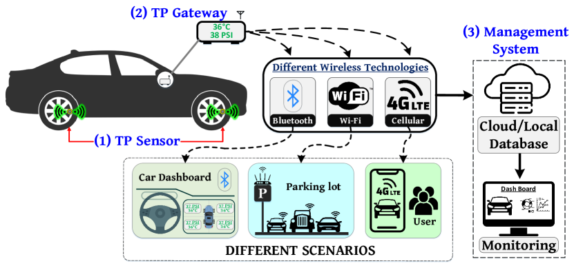
In this paper, we propose and develop a novel IoT-enabled wireless tire sensing system. The overview of the system is shown in Fig. 1. This system comprises wireless TP (temperature and pressure)111Tire temperature and pressure frequently influence each other [3, 43]. Monitoring tire condition can lead to various benefits, including accident reduction, fuel consumption minimization, driving convenience improvement, braking distance reduction, and tire lifespan extension [44, 45]. It is worth noting that certain tire monitors also incorporate inertial components [46, 47]. This paper specifically concentrates on tire sensors measuring pressure and temperature exclusively. sensors strategically positioned on each tire of the vehicle and a TP Gateway installed within the vehicle.
The TP gateway simultaneously sends data to local and cloud servers via wireless communication systems, including Wi-Fi, Bluetooth, and cellular networks, depending on the required scenarios. Specifically, this system consists of three main components: (1) Wireless TP Sensor, (2) TP Gateway, and (3) Management System, as shown in Fig. 2. These components collaborate to facilitate seamless data reception, analysis, conversion, and real-time monitoring, ensuring efficient data processing and comprehensive management.
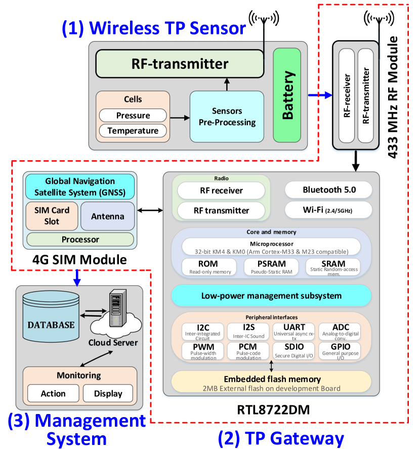
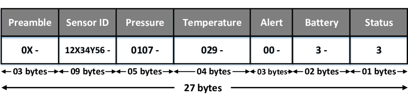
1) Wireless TP Sensor 222Currently, TP Sensor can continue to operate for several years, lasting until tire replacement, due to their low-end and uncontrollable design [48, 41, 42]. Disrupting the sensor’s energy cycle or external interference could lead to unreliable data transmission or malfunction [49, 50]. is battery powered and incorporates modules to collect accurate tire pressure and temperature data to wirelessly transmit the data through a 433 MHz antenna. The TP sensor operates on a fixed transmission duty-cycle (with the length of (in slots)) [51] and periodically transmits data containing sensor ID, pressure, temperature, alert status, battery level, and sensor status, following a predefined format, as shown in Fig. 3.
2) TP Gateway comprises three main modules, namely (a) 433 MHz RF Receiver Antenna, (b) RTL8722DM IoT Development Board, and (c) 4G SIM Module. Specifically, (a) 433 MHz RF receiver Antenna receives the encoded sensor data and transmits the signals to the RTL8722DM IoT development board for decoding into a suitable format. (b) RTL8722DM IoT Development Board is a 32-bit dual micro-controller unit and features dual-band Wi-Fi and BLE5 mesh, making it ideal for IoT applications. (c) 4G SIM Module provides extensive network coverage for 4G/LTE, 3G, and 2G bands, accurate positioning, and navigation with its built-in GNSS receiver.
3) Management system represents the connection between a physical device and the platform service, encompassing a database for local and web servers that grant access to a Graphical User Interface (GUI) and mobile application.
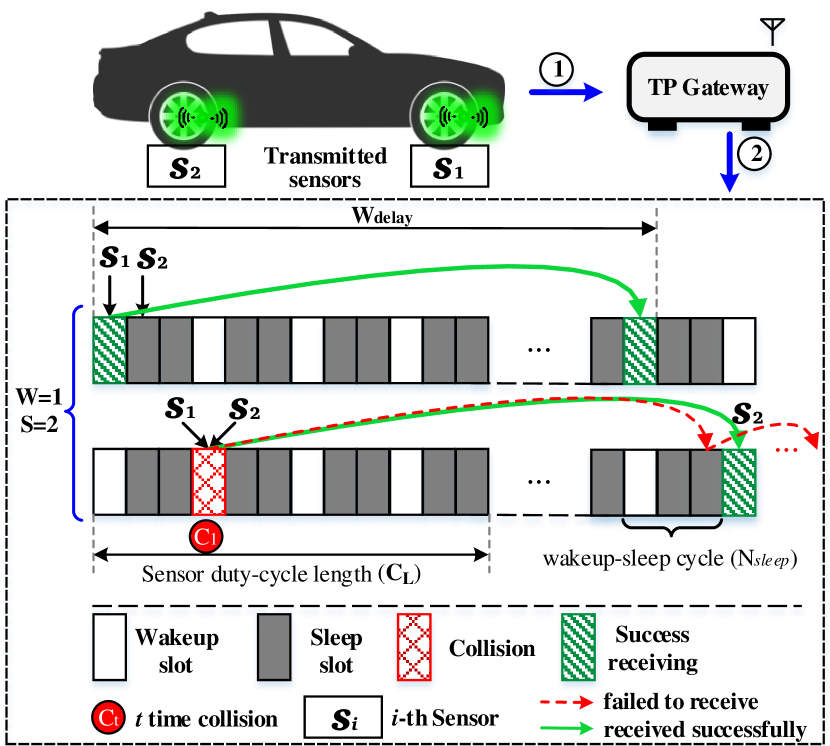
The data transmission from the sensor to the TP Gateway is illustrated in Fig. 4. In order to save system energy, the TP gateway is designed and enforced to perform wake-up (in slots) and sleep (in slots) to monitor the sensing data. Thus, it constitutes a sleep behavior with a cycle length of slots. Periodically, each sensor () transmits data every slots to the system through the 433 MHz RF antenna. The TP gateway monitors the transmitted data during the designated wakeup slot (). If the data transmission collides with another transmission (denoted by , i.e., the cross slot in the figure, where is the number of collisions and ) or occurs during the system sleeping slot, it may not be received by the system, leading to an expected delay in the receipt of the transmitted data.
In order to ensure timely data reception in the system and mitigate potential consequences of delays, it is crucial to address system reliability and data transmission delays by asking the following questions:
-
1.
Does the system exhibit a finite maximum waiting time?
-
2.
How to quantify the total expected worst transmission delay of this system considering the collision probability?
-
3.
Can it effectively determine the optimal transmission parameters, such as the minimum sensor duty-cycles and the minimum number of wakeup-sleep cycles by considering additional factors to improve the system’s reliability?
Table I presents the notations used in this paper.
| Notations | Description |
|---|---|
| Duty-cycle length of a sensor transmission | |
| The duty-cycle length of sensors | |
| Minimum number of sensor duty-cycles to successfully | |
| receive sensor transmission | |
| Total expected worst transmission delay | |
| Total number of sensors | |
| Number of wakup-sleep cycles | |
| Minimum number of wakup-sleep cycles to successfully | |
| receive sensor transmission | |
| Probability of collision | |
| Probability of success | |
| Sleeping length (in slots) | |
| The sensor in the system | |
| The sensor arrives at the time slot | |
| Worst sensor transmission | |
| Wakeup length (in slots) | |
| Worst transmission delay | |
| Wakeup-sleep cycle length |
IV The Proposed Analytic Scheme
In this section, we present an analytic scheme for determining the worst transmission delay () according to the worst sensor transmission () and minimum number of wakeup-sleep cycles (). In order to identify and , we considered various combinations of sleeping () slots, where wakeup is fixed as one slot for scheduling data in order to optimize energy consumption of the system. The scheme includes the number of transmitting sensors (), the number of wakeup-sleep cycles (), the sensor duty-cycle length (), and the worst sensor transmission .
IV-A Analytic Scheme
In this scheme, we consider two cases: is when whereas is when . Additionally, we also consider sensor transmission collision scenarios to quantify the total expected worst transmission delay .
First, we need to find the sensor incurring the worst transmission delay. Without loss of generality, we assume it first arrives at the slot, denoted by , where . The initial step involves identifying whether the sensor can be received under the wakeup-sleep operations or not. We consider the wakeup-sleep cycle starting with a wakeup slot. Then, finding the worst sensor transmission can be modeled as the scenario where a sensor arrives at the -th slot but fails to receive until several duty-cycles passed, i.e., , and is finally received at a slot over several wakeup-sleep cycles, i.e., . This is expressed as follows.
| (1) | |||
Here, and are the minimum number of sensor duty-cycles and minimum number of wakeup-sleep cycles that a sensor transmission arrives to meet a wakeup slot, respectively.
In the following, we show that exists only when the sensor duty-cycle length and the wakeup-sleep cycle length are relative prime. This is expressed in Theorem 2:
Theorem 1.
The system experiences worst sensor transmission upon successful sensor transmission reception, if
| (2) |
We employ the following Lemmas to constitute Theorem 2.
Lemma 1.1.
The system exists a feasible number of sensor duty-cycles and number of wakeup-sleep cycles to successfully receive all possible arrivals of sensor transmissions if and are relative prime, i.e., if , it exists minimal integers and that satisfies the equation for all .
Proof.
We use a direct proof method as follows. First, we rewrite Eq. (1) as follows:
| (3) |
Since , it means that and can be represented as a linear combination resulting in according to Bézout’s theorem [52], i.e.,
where . Thus, for each , we can find an integer multiple of and to satisfy Eq. (3), i.e.,
| (4) | ||||
This means that and have feasible solutions to satisfy Eq. (1) when and for all . Since , have multiple pairs, by well-ordering principle [53], it exists a pair incurring the minimal and positive solutions of and to satisfy. Under this condition, the system has a ”finite” waiting time to receive all possible sensor transmissions. ∎
Lemma 1.2.
When the system has a finite waiting time, the minimum number of sensor duty-cycles and minimum number of wakeup-sleep cycles required to successfully receive the worst sensor transmissions are and when , under the condition that and and are relative prime.
Proof.
First, we show that when , it has . We use a direct proof as follows. According to Eq. (1), it can be written as
| (5) |
By applying , we have
| (6) | ||||
Because we have to ensure the result of Eq. (6) belonging to when is set up in this scheme, it means that the following equation should belong to as wall, i.e.,
| (7) |
Since , it means that Eq. (7) has to satisfy . As we know that the minimum number of sensor duty-cycles should be larger or equal to , i.e., . Thus, the smallest value of to satisfy Eq. (7) will be because and have no common factor and cannot satisfy if . Based on this result, it yields
∎
Before introducing Lemma 1.3, we show the following two corollaries first.
Corollary 1.2.1.
When the system has a finite waiting time, the minimum number of duty-cycle will not exceed , i.e., if .
Proof.
According to Eq. (5), the numerator can be separated as two parts: and .
it means that any remainder of divided by should be deducted by the remainder of divided by . Without loss of generality, we let be the remainder of divided by . The above property can be written as
| (8) |
and
| (9) |
Also, we let be the remainder of divided by , i.e., , where is a quotient. We can rewrite Eq. (8) as
| (10) |
Based on Eq. (10), Eq. (9) can be written as
| (11) |
This can conclude two important properties. First, for those satisfying Eq. (11), they have the same , i.e.,
| (12) |
Second, from Eq. (11), will not exceed . We show it as follows.
Assume there is a and we can find a to represent as , where . From Eq. (11), we can derive it as follows.
Thus, for those , the results will be congruent to that of . So, we have the minimum number of duty-cycle . ∎
Corollary 1.2.2.
For all , their corresponding series of to satisfy Eq. (5) will constitute all possible transmission arrivals.
Proof.
First, we show that for any pair of and , their corresponding and , respectively, will not be the same (i.e., ), if and , respectively.
Here, we use a contradiction proof by assuming if and then is true. This result implies that
This contradicts to the assumption of . As a result, each has its own and individual congruence .
From this result, we can conclude that when , it totally has possible outcomes of from Eq. (12) due to its individual and difference congruence . According to Eq. (12), since difference and disjoint congruence will constitute different and disjoint sensor arrivals of , i.e.,
that means that different series of for difference will be generated. Thus, all possible transmission arrivals will be constituted and any arrival can be received by a certain . ∎
Lemma 1.3.
When the system has a finite waiting time, the worst delay will be incurred by such sensor (where ), i.e., if and are relative prime, and then .
Proof.
According to Corollary 1.2.1, we know that for all , their corresponding will not exceed , i.e., . In the following, we prove this lemma by contradiction. Assume it exists a slot , which insures a delay worse than . We consider this in two cases: one is and the other is as follows.
If , assume it has the largest value to incur the maximal delay with the maximal (because ). From Eq. (1), we have
which means that it is less than the delay incurred by with (by applying the results of Lemma 1.2). This is contradicted to the assumption.
For , we first combine it with and represent them as the continuous integers (where ). According to Eq. (9), since are continuous integers, it will have different remainders when is divided by and thus results in different congruences . This means that each has an individual . Since has been proved in Lemma 1.2 that it is with , it means that the other (where , except for ) has the largest value .
Therefore, if we want to find another worst delay from Eq. (1), we have to use the maximum with the maximum possible value . Then, the delay will be
which means that it is less than the delay incurred by with (by applying the results of Lemma 1.2). This is contradicted to the assumption. Thus, the worst delay will be incurred by . ∎
Lemma 1.4.
The system has an ”infinite” waiting time to receive all the sensors if and are not relative prime, i.e., if , it exists at least one slot that cannot satisfy .
Proof.
Since , it implies the existence of a greatest common factor that satisfies and . Then, we rewrite Eq. (1) as follows:
| (13) |
In Eq. (13), the right hand side has a factor of due to and . Thus, the left hand side of Eq. (13) should have a factor of as well according to the prime factorization, i.e.,
and thus . However, since ranges from to , these exists at least one value does not satisfy Eq. (1). For example, cannot satisfy because for any . Thus, it cannot ensure all possible transmissions to be received and incurs an “infinite” waiting time. ∎
Now, we investigate the worst transmission delay for such sensor , denoted as , and then extend this analysis to evaluate the expected total worst transmission delay, denoted as , considering the conditional probability .
Lemma 1.5.
The worst transmission delay incurring by the wakeup-sleep operation can be obtained by .
Proof.
Theorem 2.
For any sensor transmission , the system has a total expected worst transmission delay with times collision, where
| (14) | |||
Proof.
Suppose we have sensors to transmit in the system and each sensor randomly chooses a time slot to transmit within a duty-cycle in the first round without pre-defined rules or synchronization, the probability of collision for the worst sensor transmission being received at slot is given by
| (15) |
where is the successful probability without collision. To calculate , we consider the case that any other sensors choose a slot different than that one chosen by sensor . Since there are sensors and time slots available for all transmissions, the probability that sensor arrives but the remaining sensors choose other time slots will be
Thus, if sensor is not received at time slot and poses times of collisions before being received successfully, it will incur a total delay consisting of the sum of previous collision delays and the last successful reception delay. Mathematically, this total delay is given by
The probability of this total delay333 Note that if the system does not receive a sensor over slots, the system will re-activate such sensor to randomly transmit again to avoid such sensor being collided by the same pattern., denoted as , is determined by the probability of encountering a collision , raised to the power of , multiplied by the probability of successful reception , and it is with a probability given by
Therefore, using this result and Lemma 1.5, we can derive the total expected transmission delay, denoted as , as follows:
∎
In conclusion, Theorem 2 and Lemmas 1.1 1.4 are used to determine that the system has a finite delay or not, while Theorem 2 and Lemmas 1.5 are used to calculate the total expected worst transmission delay .
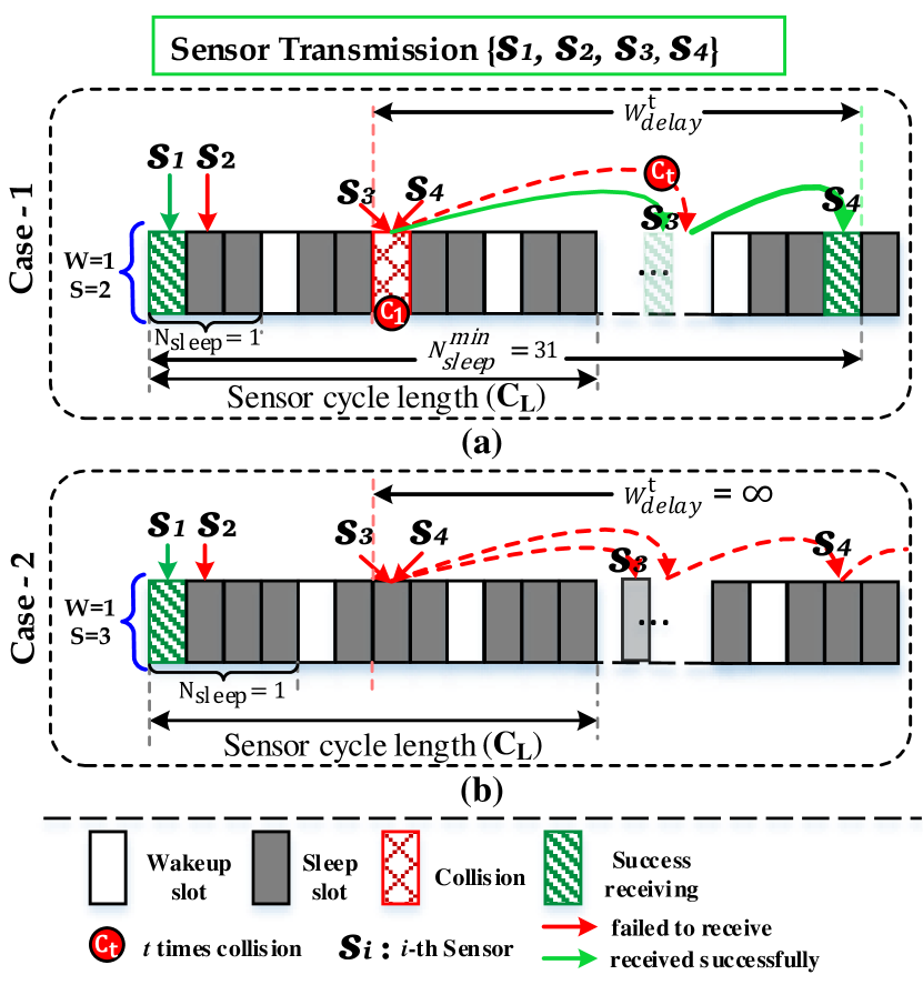
Below, we give two examples in Fig. 5 to clarify the analytic results. In the Fig. 5(a), considering , we assume that and . Based on the analytic scheme, because , we have . This implies that the sensor arriving at the slot experiences the longest transmission delay of with and .
On the other hand, in Fig. 5(b), considering . Since , the worst transmission does not exist. Therefore, it has an infinite waiting time to receive all sensors in such system.
V Performance Evaluation
In this section, we conduct both the field trial experiments and mathematical analysis to validate the effectiveness of the system. The performance evaluations, collectively referred to as Mathematical Analysis and Real-time Experiment with different parameters of where and is fixed as , to demonstrate the efficiency and effectiveness of our proposed system. It is important to note that there has been no previous work specifically addressing TP sensor with sleep operation and transmission delay, making our study the first to comprehensively investigate this critical aspect of TP sensor performance.
To simulate a realistic range of TP sensor counts for passenger vehicles and heavy-weight logistic trucks, trailers, and flatbeds, we considered sensors in our simulations. This range encompasses the typical number of sensors found on passenger vehicles ( to wheels) [54] and heavy-weight logistic trucks, trailers, and flatbeds ( to wheels) [54]. Note that the experiments will demonstrate the performance results even if the system is overloaded (i.e., , where [51]).
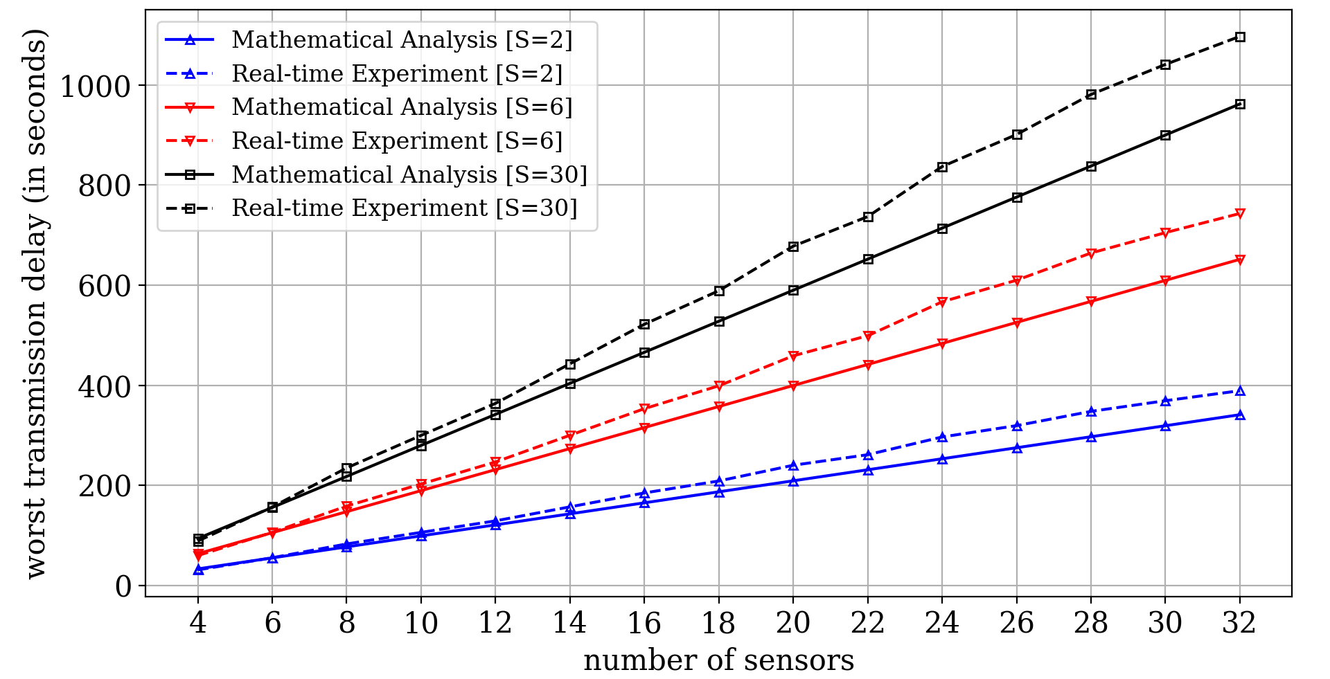
V-A Worst Transmission Delay
Fig. 6 shows the worst transmission delay (in seconds) experienced by the system for different numbers of sensors transmitting. As the number of transmitting sensors increases, the delay also increases due to frequent collisions of sensor transmissions. Note that all the pair results of mathematical and experiment analysis are consistent. Specifically, Mathematical Analysis [S=2] shows the lowest transmission delay due to a higher number of total wakeup slots per cycle length, allowing more data to be received in the system.
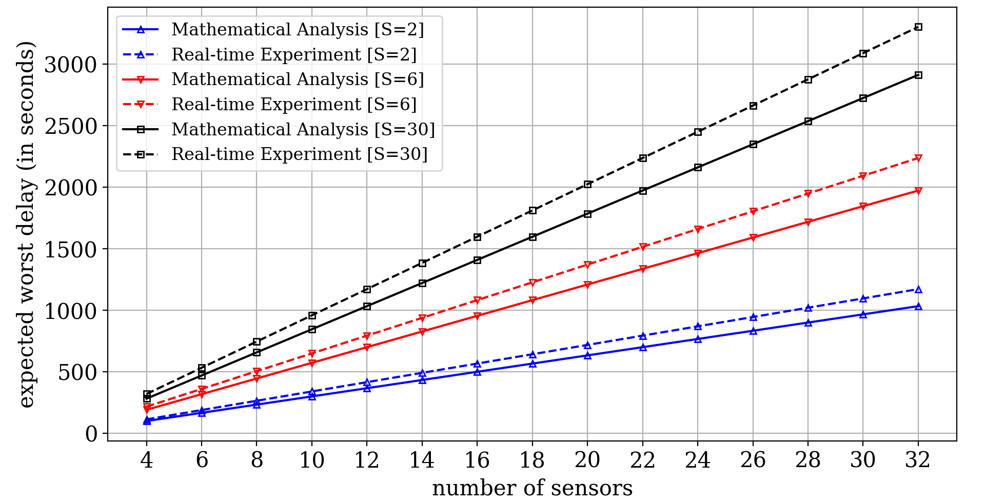
V-B Expected Worst Transmission Delay
Fig. 7 shows the expected worst transmission delay (in seconds) received in the system for different numbers of sensors transmitting, where . Based on different numbers of transmitting sensors in the system, it is shown that the expected delay of Real-time Experiment is always higher than Mathematical Analysis. This is due to a higher collision probability with an increasing number of transmitting sensors, resulting in a higher expected worst transmission delay.
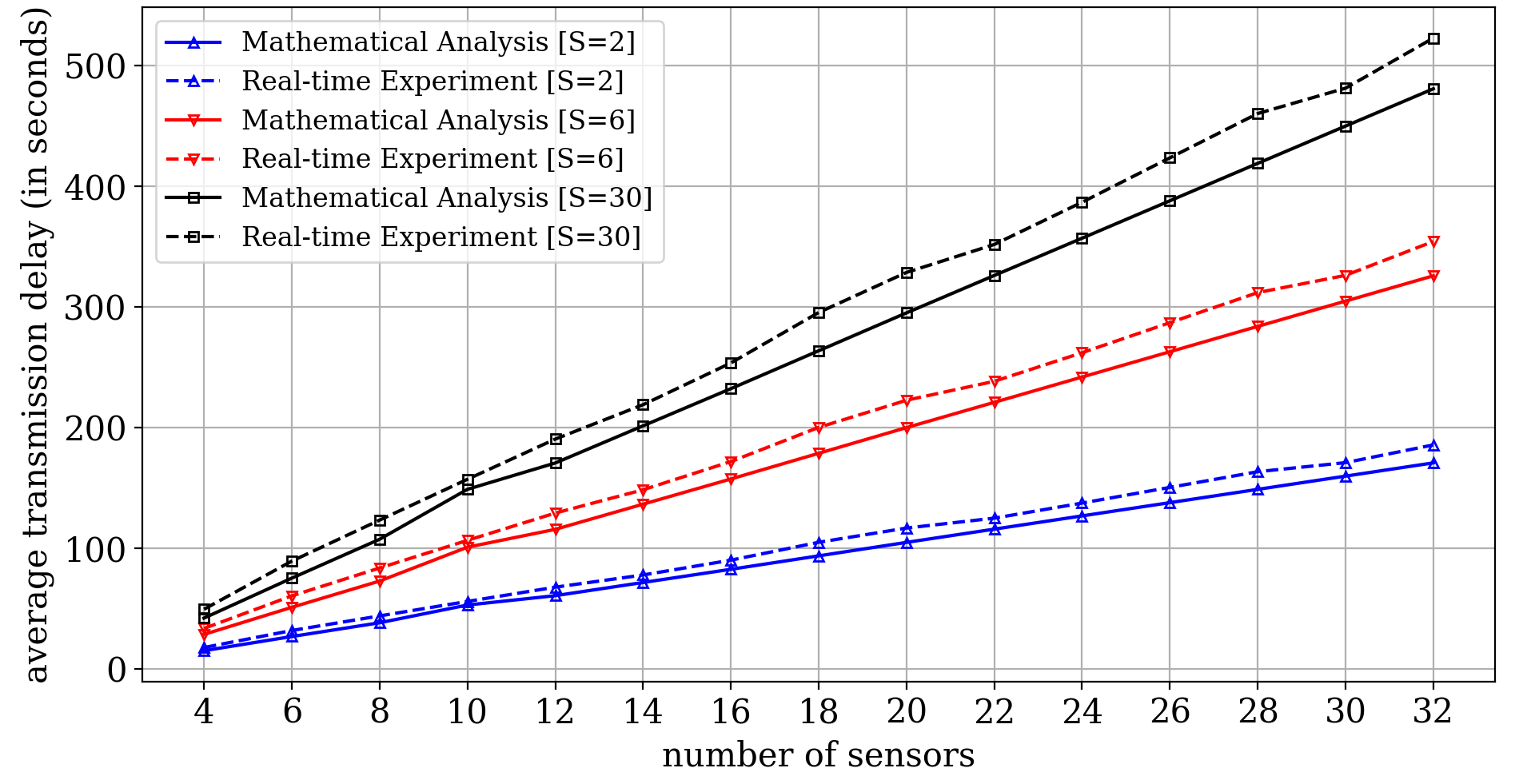
V-C Average Transmission Delay
Fig. 8 shows the average transmission delay (in seconds) received in the system for different numbers of sensors transmitting. Real-time Experiment results show the worst average results as they’re based on real-time data with higher collision probabilities, which causes a higher average transmission delay when considering the higher number of sensors transmitting per . Mathematical Analysis [S=2] results are the lowest and most efficient due to the maximum number of total wakeup slots per cycle length among all other compared schemes.
From Fig. 6 to Fig. 8, we can observe that for vehicles with fewer tires (e.g., to wheels), a shorter sleep cycle length (e.g., ) can facilitate the reception of all sensor data. For those special large vehicles such as trucks, trailers, and flatbeds with a larger number of wheels (e.g., wheels), the individual receivers will be recommended for the detached ones to facilitate the data reception.
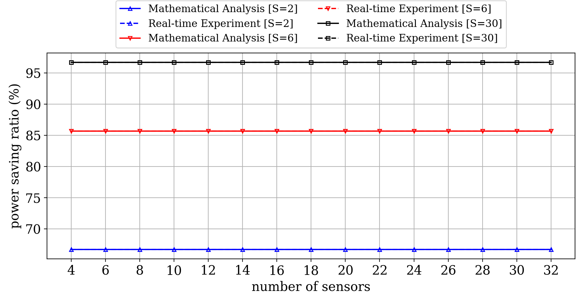
V-D Power Saving Ratio
The power saving ratio is calculated based on various numbers of transmitting sensors, where . As depicted in Fig. 9, all the schemes exhibit power-saving ratios ranging from 66.7% to 96.7% for S=2 to S=30, respectively. Even as the number of sensors increases, the power-saving ratio remains constant for each specific value of S due to the static nature of wake-up slots in the system. Real-time Experiment [S=2] demonstrates the lowest power saving ratio among all the schemes, primarily due to the fewest number of sleep slots.
| Applications | Sensors | Wireless Channel | Trans. Interval (in ms) | Delay Requirements (in ms) | Energy Consumption | *Suggested Parameters | ||
|---|---|---|---|---|---|---|---|---|
| Energy Issue? | Applicable or not? | |||||||
| ABS [45] | Wheel inertial | 5 GHz | 100200 | 150 | Yes | Yes | 150 | 10 |
| ESC [37] | Wheel inertial | 5 GHz | 100300 | 200 | Yes | Yes | 200 | 12 |
| PAS [34] | Ultrasonic | 433 MHz | 200500 | 350 | Yes | Yes | 350 | 22 |
| OSS [18] | PIR | 5 GHz | 100300 | 200 | Yes | Yes | 200 | 12 |
| LDW [40] | Radar, Infrared | 2.4 GHz | 100500 | 300 | Yes | Yes | 300 | 20 |
-
* The parameters are based on proposed analytic scheme.
-
ABS: Anti-lock Braking System; ESC: Electronic Stability Control; PAS: Parking Assist Systems; OSS: Occupancy Sensor System; LDW: Lane Departure Warning.
V-E Cumulative Correctness Rate (CCR)
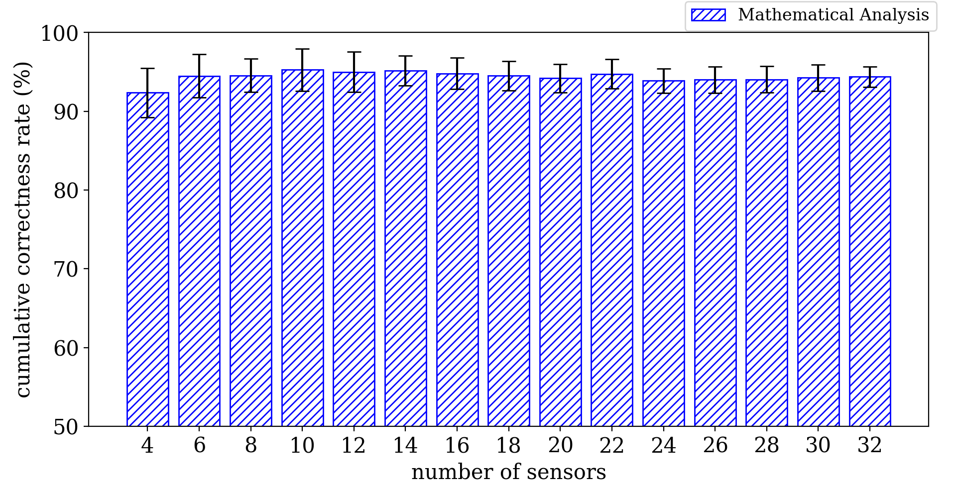
Finally, the correctness rate, the ratio of the theoretical values derived from the Mathematical Analysis (Fig. 10) to the corresponding Real-time Experiment values for Worst Transmission Delay and Average Transmission Delay. CCR is defined as:
where and represent the average values of the three aforementioned metrics in the Mathematical Analysis and the Real-time Experiment, respectively. The Mathematical Analysis achieved a significantly higher CCR (over ), demonstrating the analytic scheme’s consistency in replicating real-world behavior and its overall reliability in delivering accurate values.
V-F Discussion of Comparison and Analysis with Other Applications
Table II illustrates the potential applicability of the proposed system in various wireless sensor-based applications within intelligent vehicles, including the Anti-lock Braking System (ABS) [45], Electronic Stability Control (ESC) [37], Parking Assist Systems (PAS) [34], Occupancy Sensor System (OSS) [18], and Lane Departure Warning (LDW) [40]. We highlight a common challenge of high energy consumption resulting from frequent data transmissions (ranging from to slots, with each slot lasting milliseconds) across all applications. A key advantage of our proposed system lies in its adaptability to address such challenges. If adopting our approach on these applications, we suggest setting the parameters of the proposed scheme for ABS, ESC, PAS, OSS, and LDW at , , , , and slots, respectively, with sleep lengths set as , , , , and slots, respectively, to potentially balance transmission delays and energy consumption, both critical factors safety-critical systems. By employing our analytic scheme to analyze data and determine delays, it has the potential to mitigate the issue of high energy consumption while ensuring the seamless operation of applications.
VI System Demonstration
Intelligent vehicles rely on the IoT-enabled WTSS, a critical component that utilizes various IoT and wireless technologies to facilitate effective and efficient real-time monitoring. This section delves into its applications and demonstrates its deployment across diverse IoT and wireless technologies to achieve real-time monitoring capabilities. Note that Table III summarizes a comparative analysis of existing wireless tire sensing systems. We can say that our system has more features and more comprehensive functions than traditional systems.
| Ref.& Year | Wireless technology | Network type | Power consumption | Wireless range | Live geo-location | Storage (local/cloud) | Energy conservation | Cost | Delay analysis |
|---|---|---|---|---|---|---|---|---|---|
| 2019 [31] | Bluetooth | WPAN | Low | Short | No | Local | No | Low | No |
| 2019 [32] | Wi-Fi | WLAN | High | Medium | No | Cloud | No | High | No |
| 2020 [33] | LoRaWAN | LoRaWAN | High | Short | Yes | Cloud | No | High | No |
| 2021 [34] | Cellular | WWAN | High | Long | Yes | Cloud | No | Medium | No |
| 2021 [35] | - | - | High | - | No | - | No | Medium | No |
| 2022 [36] | Bluetooth | WPAN | Low | Short | No | Local | No | Medium | No |
| 2022 [37] | Zigbee | WPAN | Low | Short | No | Cloud | No | Medium | No |
| Proposed System | Bluetooth, Wi-Fi & Cellular | WPAN, WLAN & WWAN | Low | Long | Yes | Local & Cloud | Yes | Medium | Yes |
VI-A Overview and Working Scenario of IoT-Enabled WTSS
The proposed IoT-enabled WTSS system can manage real-time data for intelligent vehicles, making it suitable for organizations with small or large parking spaces. This includes residential neighborhoods, local parks, universities, airports, stadiums, business parks, and large automobile industries. Fig. 11 illustrates the IoT-enabled WTSS system, which utilizes multiple wireless technologies for various purposes, including 1) Bluetooth for mobile app connectivity, 2) Wi-Fi for industrial parking areas, and 3) 4G cellular for long-distance communication and real-time vehicle location tracking. The system captures and processes tire pressure and temperature data from wireless TP sensors installed on each tire of the intelligent vehicle, which is transmitted wirelessly to the TP Gateway for decoding and storage in the proposed cloud-based management system’s database. The system’s GUI dashboard provides real-time and historical data analysis, including vehicle type, parking lot, sensor positions, live geo-location, and other insights.
VI-B IoT-Enabled Modules and Components
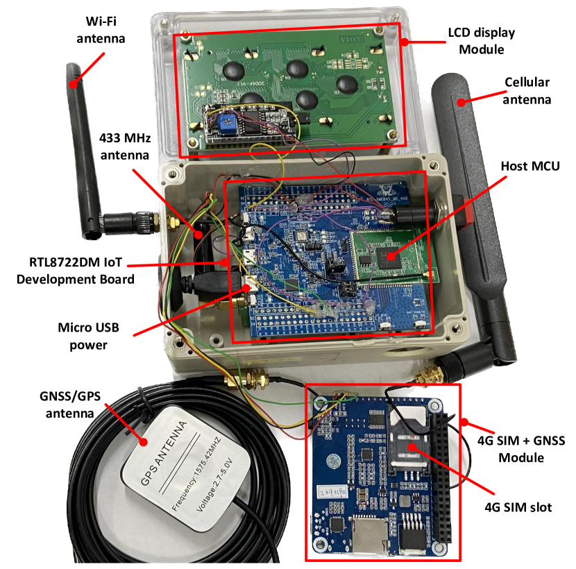
The prototype of our system has been developed and verified. Fig. 12 shows the various parts of the proposed TP Gateway. The TP Gateway is the data processing source of our proposed IoT-enabled WTSS system. To gather tire pressure, temperature, and current status of sensors, we have integrated the device with multiple modules, including RTL8722DM development board, I2C LCD, 4G SIM module, host microcontroller, 433 MHz antenna, Wi-Fi antenna, cellular antenna, and GNSS/GPS antenna.
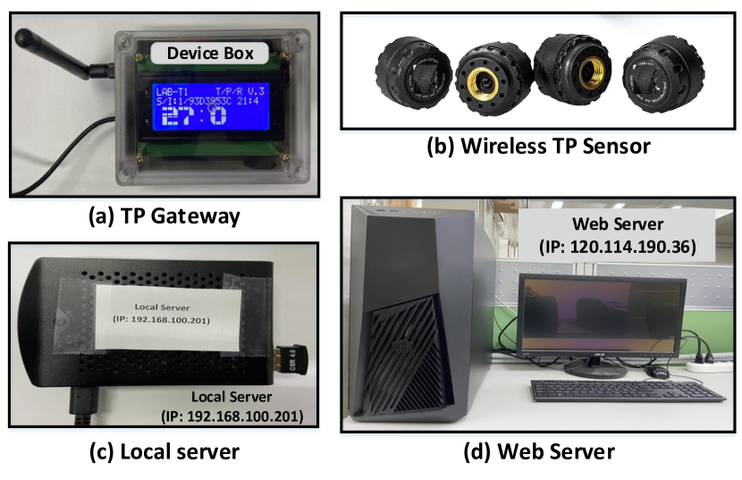
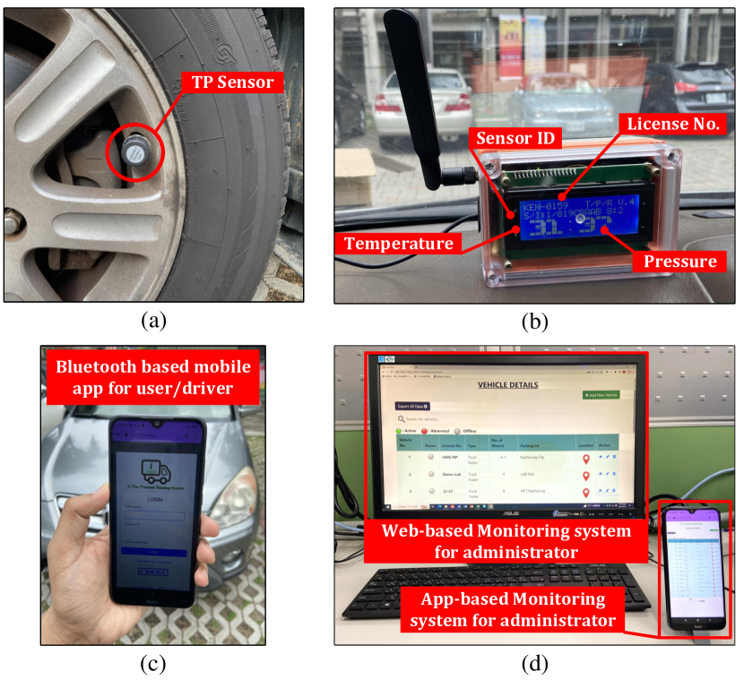
The portable device, shown in Fig. 13(a), has a box shape and features various wireless technologies that allow it to communicate with multiple devices simultaneously. It also includes a push button for activating the I2C LCD display. Fig. 13(b) illustrates 3V lithium battery-powered wireless TP sensors that gather tire pressure and temperature data with high accuracy. The module collects and transmits data through the radio frequency transmitter to the 433 MHz antenna. A local server based on Raspberry Pi4 and a web server based on Apache HTTP v3.3.0 is installed on our surveillance server. Fig. 13(c) and (d) depict the hardware configuration of the local and web servers, respectively.
The TP Gateway is an IoT-enabled real-time system designed to collect and process tire pressure and temperature data from wireless TP sensors installed on the tires of intelligent vehicles. The gateway is an important technology for the automotive industry as it enables real-time data processing, which leads to improved safety, better fuel efficiency, and longer tire life. By employing multiple wireless technologies for data transmission, it can be highly efficient and reliable. Overall, the TP Gateway can help prevent accidents and reduce maintenance costs, making it a valuable asset for fleet management and individual vehicle owners alike.
VI-C Cloud-Based Management System
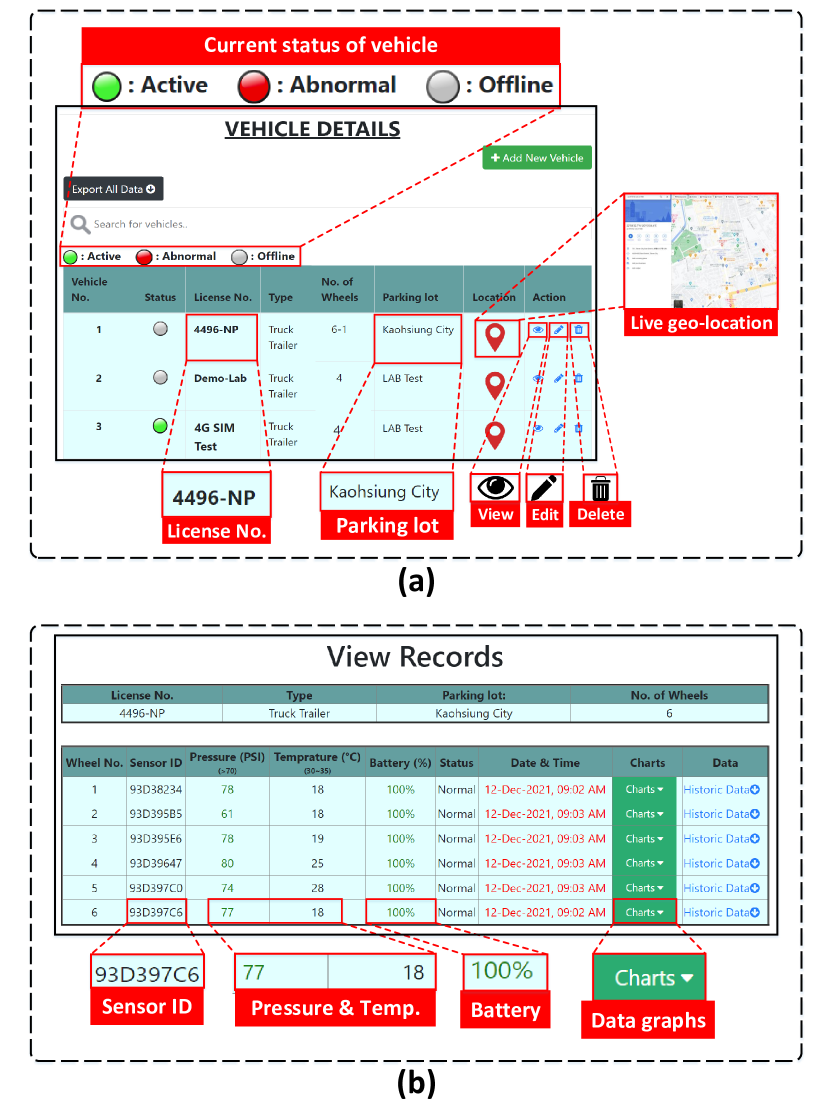
Our graphical user interface (GUI) is developed in HTML, php, JavaScript and CSS. Fig. 14 shows different snapshots of GUI. Fig. 14(a) shows all the listed vehicles with their status, vehicle type, number of wheels with attached sensors, parking lot, and live geo-location. The user interface allows the user to define a sensor by inserting its ID information and fetches real-time sensor information from the database while keeping it updated. Fig. 14(b) displays the vehicle record for each individual vehicle, which includes sensor ID, pressure, temperature, battery status, accurate time of data update, and charts for historical data.
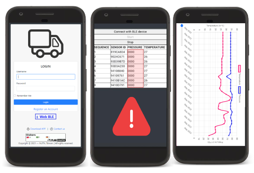
Fig. 15 shows snapshots of an Android-based mobile app. The mobile app can fetch real-time data using Bluetooth technology without the internet or over the internet. The mobile app features an SOS emergency sound alarm for abnormal tire status detection to notify the user.
VII Conclusion and Future Work
In this paper, we have developed and validated an efficient IoT-enabled wireless tire sensing system (WTSS), addressing the issue of worst transmission delay for any sensor received while considering energy savings. Our analytic scheme effectively evaluates factors affecting transmission and identifies the worst transmission delay based on different wakeup-sleep periods and collision probabilities, leading to higher energy efficiency. The real-time WTSS system, with its wireless technologies, cloud-based management system, and mobile app, offers comprehensive data insights and instant alerts to avoid accidents and boost vehicle efficiency. The effectiveness of the proposed scheme is verified by analysis, experimentation, and simulation results. The scheme effectively addresses the worst transmission delay for sensor transmission, providing a reliable and efficient solution for real-time monitoring of tire status in intelligent vehicles. This will be valuable for developers working on real-time applications for logistic trucks where minimizing sensor transmission delays is crucial.
For future work, we will further consider the energy issue of the transmitter in the WTSS. We plan to develop a new prototype of sensor transmitters with an energy-saving mechanism, enabling a more in-depth analysis of the relationship between energy consumption and delay. This initiative aims to extend the sensors’ lifetime while ensuring the immediacy of tire pressure monitoring.
References
- [1] S. Mishra and J.-M. Liang, “Design and Analysis for Wireless Tire Pressure Sensing System,” in International Computer Symposium (ICS), Taoyuan, Taiwan, 2022, pp. 599–610.
- [2] M. Germer, U. Marschner, and A. Richter, “Energy Harvesting for Tire Pressure Monitoring Systems From a Mechanical Energy Point of View,” IEEE Internet of Things Journal, vol. 9, no. 10, pp. 7700–7714, 2022.
- [3] X. Wang, Z. Chen, W. Cao, G. Xu, L. Liu, S. Liu, H. Li, X. Shi, Q. Song, Z. Xiao, and C. Sun, “Artificial Neural Network-Based Method for Identifying Under-Inflated Tire in Indirect TPMS,” IEEE Access, vol. 8, pp. 213 799–213 805, 2020.
- [4] National Highway Traffic Safety Administration (NHTSA), “Federal Motor Vehicle Safety Standard (FMVSS): Light Vehicle Brake Systems,” https://www.govinfo.gov/app/details/CFR-2022-title49-vol6/CFR-2022-title49-vol6-sec571-135/summary, accessed on March 9, 2024.
- [5] Economic Commission for Europe of the United Nations (UN/ECE), “Regulation No 141 — Uniform provisions concerning the approval of vehicles with regard to their Tyre Pressure Monitoring Systems (TPMS) [2018/1593],” http://data.europa.eu/eli/reg/2018/1593/oj, accessed on March 9, 2024.
- [6] The Ministry of Land, Transport and Maritime Affairs, “Automobile ESC/TPMS becomes mandatory,” http://www.puntofocal.gov.ar/notific_otros_miembros/kor286_t.pdf, 2010, accessed on March 9, 2024.
- [7] N. Dasanayaka and Y. Feng, “Analysis of Vehicle Location Prediction Errors for Safety Applications in Cooperative-Intelligent Transportation Systems,” IEEE Transactions on Intelligent Transportation Systems, vol. 23, no. 9, pp. 15 512–15 521, 2022.
- [8] Z. Ye, Y. Wei, W. Zhang, and L. Wang, “An efficient real-time vehicle monitoring method,” IEEE Transactions on Intelligent Transportation Systems, vol. 23, no. 11, pp. 22 073–22 083, 2022.
- [9] L. Wei, X. Wang, L. Li, L. Yu, and Z. Liu, “A Low-Cost Tire Pressure Loss Detection Framework Using Machine Learning,” IEEE Transactions on Industrial Electronics, vol. 68, no. 12, pp. 12 730–12 738, 2021.
- [10] A. A. Khan, C. Wechtaisong, F. A. Khan, and N. Ahmad, “A cost-efficient environment monitoring robotic vehicle for smart industries,” Computers, Materials & Continua, vol. 71, no. 1, pp. 473–487, 2022.
- [11] N. Sharma and R. D. Garg, “Real-Time IoT-Based Connected Vehicle Infrastructure for Intelligent Transportation Safety,” IEEE Transactions on Intelligent Transportation Systems, vol. 24, no. 8, pp. 8339–8347, 2023.
- [12] Y. Qin, H. Xu, S. Li, D. Xu, W. Zheng, W. Wang, and L. Gao, “Dual-mode flexible capacitive sensor for proximity-tactile interface and wireless perception,” IEEE Sensors Journal, vol. 22, no. 11, pp. 10 446–10 453, 2022.
- [13] A. J. C. D. S. M. A. Fan Tong, Derek Wolfson, “Energy consumption and charging load profiles from long-haul truck electrification in the United States,” Environmental Research: Infrastructure and Sustainability, vol. 1, no. 2, p. 025007, 2021.
- [14] S. Madichetty, A. J. Neroth, S. Mishra, and B. C. Babu, “Route Towards Road Freight Electrification in India: Examining Battery Electric Truck Powertrain and Energy Consumption,” Chinese Journal of Electrical Engineering, vol. 8, no. 3, pp. 57–75, 2022.
- [15] B. Al-Hanahi, I. Ahmad, D. Habibi, and M. A. S. Masoum, “Charging Infrastructure for Commercial Electric Vehicles: Challenges and Future Works,” IEEE Access, vol. 9, pp. 121 476–121 492, 2021.
- [16] Z. Yi, B. Yang, W. Zhang, Y. Wu, and J. Liu, “Batteryless Tire Pressure Real-Time Monitoring System Driven by an Ultralow Frequency Piezoelectric Rotational Energy Harvester,” IEEE Transactions on Industrial Electronics, vol. 68, no. 4, pp. 3192–3201, 2021.
- [17] Z. Meng, Y. Liu, N. Gao, Z. Zhang, Z. Wu, and J. Gray, “Radio Frequency Identification and Sensing: Integration of Wireless Powering, Sensing, and Communication for IIoT Innovations,” IEEE Communications Magazine, vol. 59, no. 3, pp. 38–44, 2021.
- [18] M. Won, “Intelligent Traffic Monitoring Systems for Vehicle Classification: A Survey,” IEEE Access, vol. 8, pp. 73 340–73 358, 2020.
- [19] A. Gharamohammadi, A. Khajepour, and G. Shaker, “In-Vehicle Monitoring by Radar: A Review,” IEEE Sensors Journal, vol. 23, no. 21, pp. 25 650–25 672, 2023.
- [20] L. Manjakkal, S. Mitra, Y. R. Petillot, J. Shutler, E. M. Scott, M. Willander, and R. Dahiya, “Connected Sensors, Innovative Sensor Deployment, and Intelligent Data Analysis for Online Water Quality Monitoring,” IEEE Internet of Things Journal, vol. 8, no. 18, pp. 13 805–13 824, 2021.
- [21] C. Chen, K. Ota, M. Dong, C. Yu, and H. Jin, “WITM: Intelligent Traffic Monitoring Using Fine-Grained Wireless Signal,” IEEE Transactions on Emerging Topics in Computational Intelligence, vol. 4, no. 3, pp. 206–215, 2020.
- [22] C. Zhang, J. He, X. Yan, Z. Liu, Y. Chen, and H. Zhang, “Exploring relationships between microscopic kinetic parameters of tires under normal driving conditions, road characteristics and accident types,” Journal of safety research, vol. 78, pp. 80–95, 2021.
- [23] K. Drozd, S. Tarkowski, J. Caban, A. Nieoczym, J. Vrábel, and Z. Krzysiak, “Analysis of Truck Tractor Tire Damage in the Context of the Study of Road Accident Causes,” Applied Sciences, vol. 12, no. 23, p. 12333, 2022.
- [24] S. M. Karim, Y. Rahman, M. A. Hai, and R. Mahfuza, “Tire Wear Detection for Accident Avoidance Employing Convolutional Neural Networks,” in 8th NAFOSTED Conference on Information and Computer Science (NICS), Hanoi, Vietnam, 2021, pp. 364–368.
- [25] P. Lin and M. Tsukada, “Model predictive path-planning controller with potential function for emergency collision avoidance on highway driving,” IEEE Robotics and Automation Letters, vol. 7, no. 2, pp. 4662–4669, 2022.
- [26] E. Artetxe, O. Barambones, I. Calvo, P. Fernández-Bustamante, I. Martin, and J. Uralde, “Wireless Technologies for Industry 4.0 Applications,” Energies, vol. 16, no. 3, p. 1349, 2023.
- [27] O. Seijo, X. Iturbe, and I. Val, “Tackling the Challenges of the Integration of Wired and Wireless TSN With a Technology Proof-of-Concept,” IEEE Transactions on Industrial Informatics, vol. 18, no. 10, pp. 7361–7372, 2022.
- [28] M. I. Tawakal, M. Abdurohman, and A. G. Putrada, “Wireless monitoring system for motorcycle tire air pressure with pressure sensor and voice warning on helmet using fuzzy logic,” in International Conference on Software Engineering & Computer Systems and 4th International Conference on Computational Science and Information Management (ICSECS-ICOCSIM), Pahang, Malaysia, 2021, pp. 47–52.
- [29] D. Hou, Y. Zhao, Y. Wang, D. Gu, and Z. Xi, “ID Calibration Device Design for Vehicle Tire Pressure Monitoring System Based on Bluetooth Communication,” Procedia Computer Science, vol. 202, pp. 223–227, 2022.
- [30] W.-H. Chang, R.-T. Juang, M.-H. Huang, and M.-F. Sung, “Implementation of Tire Status Estimation Using Hall Sensor and G-Sensor,” in IEEE/ACIS 22nd International Conference on Software Engineering, Artificial Intelligence, Networking and Parallel/Distributed Computing (SNPD), Taichung, Taiwan, 2021, pp. 102–105.
- [31] H. Fechtner, U. Spaeth, and B. Schmuelling, “Smart Tire Pressure Monitoring System with Piezoresistive Pressure Sensors and Bluetooth 5,” in IEEE Conference on Wireless Sensors (ICWiSe), Penang, Malaysia, 2019, pp. 18–23.
- [32] J. M. S. Waworundeng, D. Fernando Tiwow, and L. M. Tulangi, “Air Pressure Detection System on Motorized Vehicle Tires Based on IoT Platform,” in 1st International Conference on Cybernetics and Intelligent System (ICORIS), Bali, Indonesia, 2019, pp. 251–256.
- [33] P. Ferrari, E. Sisinni, D. F. Carvalho, A. Depari, G. Signoretti, M. Silva, I. Silva, and D. Silva, “On the use of LoRaWAN for the Internet of Intelligent Vehicles in Smart City scenarios,” in IEEE Sensors Applications Symposium (SAS), Kuala Lumpur, Malaysia, 2020, pp. 1–6.
- [34] S. Hussain, U. Mahmud, and S. Yang, “Car e-talk: An iot-enabled cloud-assisted smart fleet maintenance system,” IEEE Internet of Things Journal, vol. 8, no. 12, pp. 9484–9494, 2021.
- [35] S. Formentin, L. Onesto, T. Colombo, A. Pozzato, and S. M. Savaresi, “h-tpms: a hybrid tire pressure monitoring system for road vehicles,” Mechatronics, vol. 74, p. 102492, 2021.
- [36] A. Pangestu, I. Sodikin, M. Yusro, R. Sapundani, R. R. Al Hakim, and S. Wilyanti, “IoT- based tire pressure monitoring system for air and temperature pressure using MPX5500D and LM35 sensor,” in IEEE 8th International Conference on Computing, Engineering and Design (ICCED), Sukabumi, West Java Indonesia, 2022, pp. 1–4.
- [37] A. Vasantharaj, N. Nandhagopal, S. A. Karuppusamy, and K. Subramaniam, “An in-tire-pressure monitoring SoC using FBAR resonator-based ZigBee transceiver and deep learning models,” Microprocessors and Microsystems, vol. 95, p. 104709, 2022.
- [38] S. Zhou, Y. Du, B. Chen, Y. Li, and X. Luan, “An Intelligent IoT Sensing System for Rail Vehicle Running States Based on TinyML,” IEEE Access, vol. 10, pp. 98 860–98 871, 2022.
- [39] M. A. Rahman, M. A. Rahim, M. M. Rahman, N. Moustafa, I. Razzak, T. Ahmad, and M. N. Patwary, “A Secure and Intelligent Framework for Vehicle Health Monitoring Exploiting Big-Data Analytics,” IEEE Transactions on Intelligent Transportation Systems, vol. 23, no. 10, pp. 19 727–19 742, 2022.
- [40] D. Katare, D. Perino, J. Nurmi, M. Warnier, M. Janssen, and A. Y. Ding, “A survey on approximate edge ai for energy efficient autonomous driving services,” IEEE Communications Surveys & Tutorials, vol. 25, no. 4, pp. 2714–2754, 2023.
- [41] Z. Márton, I. Szalay, and D. Fodor, “Convolutional Neural Network-Based Tire Pressure Monitoring System,” IEEE Access, vol. 11, pp. 70 317–70 332, 2023.
- [42] N. Xu, Y. Huang, H. Askari, and Z. Tang, “Tire Slip Angle Estimation Based on the Intelligent Tire Technology,” IEEE Transactions on Vehicular Technology, vol. 70, no. 3, pp. 2239–2249, 2021.
- [43] L. Wei, Y. Liu, X. Wang, and L. Li, “Estimation of Wheel Pressure for Hydraulic Braking System by Interacting Multiple Model Filter,” IEEE Transactions on Vehicular Technology, vol. 73, no. 1, pp. 463–472, 2024.
- [44] Y. Wang, Y. Zhang, Z. Jiang, L. Zheng, J. Chen, and J. Lu, “Prototype-Based Supervised Contrastive Learning Method for Noisy Label Correction in Tire Defect Detection,” IEEE Sensors Journal, vol. 24, no. 1, pp. 660–670, 2024.
- [45] G. Sidorenko, J. Thunberg, K. Sjöberg, A. Fedorov, and A. Vinel, “Safety of Automatic Emergency Braking in Platooning,” IEEE Transactions on Vehicular Technology, vol. 71, no. 3, pp. 2319–2332, 2022.
- [46] L. Zhang, P. Guo, Z. Wang, and X. Ding, “An Enabling Tire-Road Friction Estimation Method for Four-in-Wheel-Motor-Drive Electric Vehicles,” IEEE Transactions on Transportation Electrification, vol. 9, no. 3, pp. 3697–3710, 2023.
- [47] L. Xiong, X. Xia, Y. Lu, W. Liu, L. Gao, S. Song, and Z. Yu, “IMU-Based Automated Vehicle Body Sideslip Angle and Attitude Estimation Aided by GNSS Using Parallel Adaptive Kalman Filters,” IEEE Transactions on Vehicular Technology, vol. 69, no. 10, pp. 10 668–10 680, 2020.
- [48] P. Razmjoui, A. Kavousi-Fard, T. Jin, M. Dabbaghjamanesh, M. Karimi, and A. Jolfaei, “A Blockchain-Based Mutual Authentication Method to Secure the Electric Vehicles’ TPMS,” IEEE Transactions on Industrial Informatics, vol. 20, no. 1, pp. 158–168, 2024.
- [49] S. Salih and R. Olawoyin, “Fault Injection in Model-Based System Failure Analysis of Highly Automated Vehicles,” IEEE Open Journal of Intelligent Transportation Systems, vol. 2, pp. 417–428, 2021.
- [50] J. C. Kim, D. J. Lee, S. W. Hwang, B.-K. Ju, S. K. Yun, H.-W. Park, and J. T. Chung, “Investigation of the Cause of a Malfunction in a Display Package and Its Solution,” IEEE Transactions on Components, Packaging and Manufacturing Technology, vol. 1, no. 1, pp. 119–124, 2011.
- [51] AVE, “Ave External Sensor Specification,” http://www.avetechnology.com/index.php?unit=products&lang=en&act=view&id=89, [Online; accessed 16-November-2023].
- [52] S. McKean, “An Arithmetic Enrichment of Bézout’s Theorem,” Mathematische Annalen, vol. 379, no. 1–2, p. 633–660, Jan. 2021. [Online]. Available: http://dx.doi.org/10.1007/s00208-020-02120-3
- [53] D. MacHale, “92.30 The well-ordering principle for ,” The Mathematical Gazette, vol. 92, no. 524, pp. 257–259, 2008.
- [54] C. M. Farmer and A. K. Lund, “Rollover risk of cars and light trucks after accounting for driver and environmental factors,” Accident Analysis & Prevention, vol. 34, no. 2, pp. 0001–4575, 2002.
![[Uncaptioned image]](/html/2405.05757/assets/Image/ms011.png) |
Shashank Mishra received the Masters degree in Software Technology from the VIT University, Vellore, India in 2013. He is currently working toward the Ph.D. degree in Electrical Engineering with the Department of Electrical Engineering, National University of Tainan, Tainan, Taiwan. His research interests include resource utilization and management in Artificial Intelligence of Things (AIoT), Wireless Sensor Networks (WSNs), and Intelligent Vehicles. |
![[Uncaptioned image]](/html/2405.05757/assets/Image/liang.png) |
Jia-Ming Liang received his Ph.D. degree in Computer Science from National Chiao Tung University in 2011. He was an Assistant Research Fellow in the Department of Computer Science, National Chiao Tung University, Taiwan, from 2012 to 2015. In 2015, he was an Assistant Professor in the Department of Computer Science and Information Engineering, Chang Gung University, Taoyuan, Taiwan. Since 2020, he joined the Department of Electrical Engineering, National University of Tainan, Taiwan, where he is currently an Associate Professor. His research interests include resource management in 5G/B5G mobile networks and Artificial Intelligence of Things (AIoT). |