3D bulk field theories for 2D non-unitary ${\cal N}=1$ supersymmetric minimal models

Abstract

We propose bulk 3D ${\cal N}=4$ rank-0 superconformal field theories, which are related to 2D ${\cal N}=1$ supersymmetric minimal models, $SM(2,\cdot)$ and $SM(3,\cdot)$, via recently discovered non-unitary bulk-boundary correspondence. The correspondence relates a 3D ${\cal N}=4$ rank-0 superconformal field theory to 2D chiral rational conformal field theories. A topologically twisted theory of the rank-0 SCFT supports the rational chiral algebra at the boundary upon a proper choice of boundary condition. We test the proposal by checking several non-trivial dictionaries of the correspondence.

1 Introduction

2D rational conformal field theories (2D RCFTs) and 3D topological field theories (3D TQFTs) are the most recurring themes in theoretical and mathematical physics. They describe universal behaviors of critical phenomena in 2D statistical models and (2+1)D topological orders respectively. Mathematically, RCFTs have underlying rational chiral algebra, a.k.a rational vertex operator algebra (rational VOA). Both RCFTs and TQFTs share a rigid mathematical structure called modular tensor category (MTC), which defines a framed topological invariant of 3-manifolds and knots zbMATH04092352 ; moore1989classical ; turaev1992modular . Some substructures of the MTC are found to be ubiquitous in quantum field thories in various space-time dimensions and play a key role in recent developments of generalized symmetry, see $e.g.$ Gaiotto:2014kfa ; Bhardwaj:2017xup ; Chang:2018iay ; Heidenreich:2021xpr ; Koide:2021zxj ; Choi:2021kmx ; Kaidi:2021xfk . Based on the common MTC structure, the two topics are beautifully connected via so-called bulk-boundary correspondence zbMATH04092352 ; moore1989lectures .

There also exist non-unitary RCFTs and TQFTs. Non-unitary RCFTs arise from 2D statistical models with imaginary parameters fisher1978yang ; cardy1985conformal . Non-unitary chiral algebra also appears as a BPS subsector of supersymmetric quantum field theories (SQFTs) in higher $(D>2)$ dimensions Beem:2013sza ; Beem:2014kka ; Feigin:2018bkf ; Cheng:2018vpl ; Costello:2018fnz ; Costello:2020ndc ; Cheng:2022rqr . For most cases, however, the non-unitary chiral algebra from SQFTs are irrational Song:2017oew ; Beem:2017ooy ; Arakawa:2017fdq ; Xie:2019vzr ; Gukov:2020lqm ; Creutzig:2021ext . Recently, a physical realization of 3D non-unitary (semi-simple and finite) TQFTs is proposed through full topological twistings of an exotic class of 3D ${\cal N}=4$ superconformal field theories (SCFTs) called rank-0 SCFTs Gang:2018huc ; Gang:2021hrd .  Being rank-0 means that there are no Coulomb or Higgs branch operators in the theory and the property turned out to be crucial to support rational chiral algebra at the boundary Costello:2018swh ; Beem:2023dub ; Ferrari:2023fez . Using the physical realization of non-unitary TQFTs, the bulk-boundary correspondence has been extended to the non-unitary cases in the following way:

$$\framebox{3D rank-0 SCFT }\xrightarrow{\rm top^{\prime}l\;twistings}\framebox{3D non-unitary TQFTs}\xrightarrow{\textrm{at boundary}}\framebox{2D chiral RCFTs}$$ (1)

Refer to Gang:2023rei ; Gang:2022kpe ; Gang:2023ggt ; Ferrari:2023fez ; Dedushenko:2018bpp ; Dedushenko:2023cvd for the recent developments along the direction.

Using the underlying rigid mathematical structures, there has been efforts to classifiy RCFTs. Famously, unitary 2D CFTs with central charge $c<1$ are all classified and they form a series of RCFTs called Virasoro minimal model. The Virasoro minimal model can be further generalized to include non-unitary ones and it will be denoted by $M(p,q)$ with two coprime integers $p$ and $q$ ($2\leq p<q$). They have the Virasoro algera with certain rational values of $c$ as the underlying chiral algebra. The $M(p,q)$ is unitary if and only if $|p-q|=1$. For Lee-Yang series of the non-unitary minimal model, $M(2,q)$ with $q\in 2\mathbb{Z}_{\geq 2}+1$, the corresponding bulk rank-0 SCFTs were proposed recently Gang:2023rei . There also exist supersymmetric version of minimal models, supersymmetric minimal model $SM(p,p^{\prime})$ labeled by two integers subjected to the conditions in (2). The underlying rational chiral algebra is 2D ${\cal N}=1$ super-Virasoro algebra with certain rational values of $c$. The $SM(p,p^{\prime})$ is unitary if and only if $|p-p^{\prime}|=2$. In this paper, we propose the bulk 3D rank-0 SCFTs corresponding to the non-untary 2D supersymmeric minimal models with $p=2$ and $p=3$.

The rest of this paper is organized as follows. In section 2, we first review some basic aspects of supersymmetric minimal models and non-unitary bulk-boundary correspondence. Basic dictionaries of the correspondence are summarized in Table 1. Then, we propose the bulk ${\cal N}=4$ rank-0 SCFTs corresponding to supersymmetric minimal models $SM(p,p^{\prime})$ with $p=2,3$. For $p=2$, we present 3 distinct UV gauge theory descriptions which are claimed to be IR equivalent modulo a decoupled invertible spin-TQFT $SO(1)_{1}$, i.e. Ising spin-TQFT. The theories have ${\cal N}=4$ (resp. ${\cal N}=5$) supersymmetry in the IR for $p=3$ (resp. $p=2$). In appendix A, we also present new UV description of bulk field theories for minimal models $M(p,q)$ with $p=2$, which are claimed to be IR equivalent to the theories in Gang:2023rei modulo a decoupled invertible spin TQFT $SO(1)_{1}$, Ising spin-TQFT.

2 Bulk dual ${\cal N}=4$ rank-0 SCFTs of ${\cal N}=1$ minimal models

2.1 Supersymmetric minimal model $SM(p,p^{\prime})$ and rank-0 SCFT ${\cal T}_{(p,p^{\prime})}$

Here we review basic aspects of the minimal model $SM(p,p^{\prime})$ and the non-unitary bulk-boundary correspondence.

Supersymmetric minimal model $SM(p,p^{\prime})$

The ${\cal N}=1$ minimal model $SM(p,p^{\prime})$ is labeled by two integers, $p$ and $p^{\prime}$, satisfying

$$2\leq p<p^{\prime},\;\;p^{\prime}-p\in 2\mathbb{Z}\textrm{ and gcd}\left(p,\frac{(p^{\prime}-p)}{2}\right)=1\;.$$ (2)

Primaries ${\cal O}_{(s,t)}$ are labeled by two integers, $1\leq s\leq p-1$ and $1\leq t\leq p^{\prime}-1$, with an equivalence relation ${\cal O}_{(s,t)}={\cal O}_{(p-s,p^{\prime}-t)}$. ${\cal O}_{(s,t)=(1,1)}$ is the identity operator. Central charge $c$ and conformal dimensions $h$ of the primaries are

$$\begin{split}&c=\frac{3}{2}\left(1-\frac{2(p^{\prime}-p)^{2}}{pp^{\prime}}\right)\;,\\ &h_{(s,t)}=\begin{cases}&\frac{(p^{\prime}s-pt)^{2}-(p-p^{\prime})^{2}}{8pp^{\prime}}\;,\quad s-t\in 2\mathbb{Z}\;\;(\textrm{NS sector})\\ &\frac{(p^{\prime}s-pt)^{2}-(p-p^{\prime})^{2}}{8pp^{\prime}}+\frac{1}{16}\;,\quad\quad s-t\in 2\mathbb{Z}+1\;\;(\textrm{R sector})\end{cases}\end{split}$$ (3)

Conformal characters for NS sectors are ($s-t\in 2\mathbb{Z}$)

$$\chi_{(s,t)}=q^{h_{(s,t)}-\frac{c}{24}}\frac{(-q^{\frac{1}{2}};q)_{\infty}}{(q;q)_{\infty}}\sum_{l\in\mathbb{Z}}\left(q^{\frac{l(lpp^{\prime}+sp^{\prime}-tp)}{2}}-q^{\frac{(lp+s)(lp^{\prime}+t)}{2}}\right)\,.$$ (4)

We use following $q$-Pochhammer symbols

$$\begin{split}&(x;q)_{k}:=\prod_{n=0}^{k-1}(1-q^{n}x),\quad(x;q)_{\infty}:=\prod_{n=0}^{\infty}(1-q^{n}x),\\ &(q)_{k}:=(q;q)_{k}=\prod_{n=1}^{k}(1-q^{n}),\quad(q)_{\infty}:=(q;q)_{\infty}=\prod_{n=1}^{\infty}(1-q^{n})\;.\end{split}$$ (5)

Modular S-matrix for the ${\rm NS}$ characters is

$$S_{(s_{1},t_{1}),(s_{2},t_{2})}=\frac{2}{\sqrt{pp^{\prime}}}\left(\cos(\frac{2\pi\lambda_{1}\lambda_{2}}{4pp^{\prime}})-\cos(\frac{2\pi\bar{\lambda}_{1}\lambda_{2}}{4pp^{\prime}})\right)\;,$$ (6)

with $\lambda_{i}=pt_{i}-p^{\prime}s_{i},\bar{\lambda}_{i}=pt_{i}+p^{\prime}s_{i}$. The S-matrix determines the transformation rule of the NS characters under the modular $S$-transformation, $\tau\rightarrow-\frac{1}{\tau}$:

$$\chi_{\alpha}(\tilde{q})=\sum_{\beta}S_{\alpha\beta}\chi_{\beta}(q)\;\;\textrm{ where }q:=e^{2\pi i\tau}\textrm{ and }\tilde{q}:=e^{2\pi i(-1/\tau)}\;.$$ (7)

Here $\alpha$ and $\beta$ label the NS primaries.

3D Rank-0 ${\cal N}=4$ SCFT ${\cal T}_{(p,p^{\prime})}$

Let the ${\cal T}_{(p,p^{\prime})}$ be the bulk 3D rank-0 SCFT associated to the minimal model $SM(p,p^{\prime})$ via the non-unitary bulk-boundary correspondence:

$$\textrm{3D SCFT }{\cal T}_{(p,p^{\prime})}\xrightarrow{\rm top^{\prime}l\;A-twisting\;}\textrm{3D TQFT }{\cal T}^{\rm A}_{(p,p^{\prime})}\xrightarrow{\textrm{at boundary}}\textrm{2D RCFT }SM(p,p^{\prime}).$$ (8)

Basic dictionaries of the correspondence are summarized in the Table 1. Here $\mathbb{B}$ is a supersymmetric boundary condition of the rank-0 SCFT which becomes a holomorphic boundary condition in the A-twisted theory ${\cal T}^{\rm A}$, under which the non-unitary TQFT ${\cal T}^{\rm A}$ supports (chiral) rational conformal field theory ${\cal R}[{\cal T}^{\rm A};\mathbb{B}]$ at the boundary. Refer to Gang:2021hrd ; Gang:2023rei ; Gang:2023ggt for details and reasons behind the dictionaries. Since we are interested in the case when the boundary RCFT is a supersymmetric minimal model, we list the dictionaries for fermionic case. One crucial difference from the bosonic case is that the conformal dimensions $h_{\alpha}$ of primaries are determined modulo $1/2$, instead of $1$, from the bulk computation.

$\quad\textrm{Boundary 2D $\chi$RCFT }\mathcal{R}[{\cal T}^{A},\mathbb{B}]$	Bulk 3D rank-0 SCFT ${\cal T}$
	Bethe vacua $\{\vec{z}_{\alpha}\}_{\alpha=0}^{N-1}$
NS-sector primaries ${\cal O}_{\alpha=0,\ldots,N-1}$	or
	BPS loop operators $\{L_{\alpha}(\vec{z})\}_{\alpha=0}^{N-1}$
$(S_{0\alpha})^{-2}$	${\cal H}(\vec{z}_{\alpha},M=0,\nu=-1)$
$|S_{00}|$	$\bigl{|}{\cal Z}_{S^{3}_{b}}(M=0,\nu=-1)\bigr{|}$
${\rm min}_{\alpha}|S_{0\alpha}|$	$e^{-F}:=\bigl{|}{\cal Z}_{S^{3}_{b}}(M=0,\nu=0)\bigr{|}$
$W_{\beta}(\alpha):=S_{\alpha\beta}/S_{0\beta}$	$L_{\alpha}(\vec{z}_{\beta})$
Conformal dimension $h_{\alpha}$	$\left(\frac{{\cal F}(\vec{z}_{\alpha},M=0,\nu=-1)}{{\cal F}(\vec{z}_{\alpha=0},M=0,\nu=-1)}\right)^{2}=\exp(4\pi ih_{\alpha})$
$\chi_{\alpha}(q)=q^{h_{\alpha}-c/24}I^{L_{\alpha}}_{\rm half:\mathbb{B}}$	Half-index $I_{\rm half:\mathbb{B}}^{L_{\alpha}}(q,\eta=1,\nu=-1)$

Table 1: Basic dictionaries of non-unitary bulk boundary correspondence for fermionic case, i.e. the boundary theory is a fermionic (or spin) RCFT. Here $\{\chi_{\alpha}\}_{\alpha=0}^{N-1}$ are the conformal characters, $\textrm{Tr}q^{L_{0}-\frac{c}{24}}$, of irreducible modules associated to primaries $\{{\cal O}_{\alpha}\}$ and $\alpha=0$ corresponds to the vacuum module, i.e. ${\cal O}_{\alpha=0}$ is the identity operator. Supersymmetric quantities (${\cal H},{\cal F},{\cal Z}_{S^{3}_{b}}$ and $I^{L}_{\rm half}$) of the bulk rank-0 SCFT appearing in the table are explained in main text. $F$ is the round 3-sphere free energy Jafferis:2011zi ; Casini:2015woa .

BPS partition functions of rank-0 SCFTs

Now let us explain the supersymmetric quantities appearing in the right-hand side of the table. They can be computed using the so-called supersymmetric localization method, which is applicable to any 3D ${\cal N}=2$ theories. In terms of an ${\cal N}=2$ supersymmetry subalgebra, rank-0 SCFT has a $U(1)_{A}$ flavor symmetry whose charge $A$ is

$$A=(J_{3}^{C}-J_{3}^{H})\;,$$ (9)

where $J_{3}^{C}$ and $J_{3}^{H}$ are the two Cartans of the $SO(4)\simeq SU(2)^{C}\times SU(2)^{H}$ R-symmetry normalized as $J_{3}\in\mathbb{Z}/2$. Supersymmetric partition functions of rank-0 SCFT depends on $M$ (or $\eta$) and $\nu$ where $M$ (or $\eta$) is a (rescaled) real mass parameter (or fugacity) for the $U(1)_{A}$ symmetry and $\nu$ parametrizes the R-symmetry mixing as follows

$$R_{\nu}=(J_{3}^{C}+J_{3}^{H})+\nu(J_{3}^{C}-J_{3}^{H})\;.$$ (10)

$R_{\nu=0}$ corresponds to the superconformal R-charge. We consider 3 types of supersymmetric backgrounds on closed 3-manifolds, superconformal index Kim:2009wb ; Imamura:2011su , squashed 3-sphere partition function Kapustin:2009kz ; Jafferis:2010un ; Hama:2010av ; Hama:2011ea and twisted partition functions Benini:2015noa ; Benini:2016hjo ; Closset:2016arn ; Closset:2017zgf ; Closset:2018ghr . We also consider half-index Gadde:2013wq ; Gadde:2013sca ; Yoshida:2014ssa ; Dimofte:2017tpi defined on $D_{2}\times S^{1}$ with a proper SUSY boundary condition $\mathbb{B}$.

The superconformal index ${\cal I}_{\rm sci}(q;\eta,\nu)$ is defined as

$${\cal I}_{\rm sci}(q;\eta,\nu):=\textrm{Tr}_{{\cal H}_{\rm rad}(S^{2})}(-1)^{R_{\nu}}q^{\frac{R_{\nu}}{2}+j_{3}}\eta^{A}\;,$$ (11)

where the trace is taken over the radially quantized Hilbert-space ${\cal H}_{\rm rad}(S^{2})$, whose elements are in one-to-one with local operators of the SCFT. $j_{3}$ is the 3rd component of the Lorentz spin. Due to the $(-1)^{R_{\nu}}$ factor, there are huge cancellations and only local operators satisfying following condition could give non-vanishing contributions to the index,

$$\Delta=R_{\nu=0}+j_{3}\;,$$ (12)

where $\Delta$ is the conformal dimension. The squashed 3-sphere partition ${\cal Z}_{S^{3}_{b}}(b^{2};M,\nu)$ is defined on the following $S^{3}_{b}$ background:

$$S^{3}_{b}:=\{(z,w)\in\mathbb{C}^{2}\;:\;b^{2}|z|^{2}+b^{-2}|w|^{2}=1\}\;.$$ (13)

When $b=1$, it corresponds to the round 3-sphere. The partition function depends on the rescaled real mass parameter $M$ ($b\times$real mass) and R-symmetry mixing parameter $\nu$ only through a holomorphic combination $M+(i\pi+\frac{\hbar}{2})\nu$:

$$\mathcal{Z}_{S^{3}_{b}}(b^{2};M,\nu)=\mathcal{Z}_{S^{3}_{b}}\left(b^{2};M+(i\pi+\frac{\hbar}{2})\nu\right)\;,$$ (14)

where $\hbar:=2\pi ib^{2}$. The round 3-sphere partition function can be used in determining the correct IR superconformal R-charge via F-maximization Jafferis:2010un and in defining the $F=-\log|{\cal Z}_{S^{3}_{b}}(b^{2}=1)|$, which is a proper measure of the number of degrees of freedom in 3D CFTs Jafferis:2011zi ; Casini:2015woa .

The twisted partition function ${\cal Z}_{{\cal M}_{g,p}}(M,\nu)$ on ${\cal M}_{g,p}$, degree $p$ circle bundle over genus $g$ Riemann surface $\Sigma_{g}$, can be given in the following form

$$\begin{split}&{\cal Z}_{{\cal M}_{g,p\in 2\mathbb{Z}}}(M,\nu)=\sum_{\vec{z}_{\alpha}\in{\cal S}_{\rm BE}(M,\nu)\;}\left({\cal H}(\vec{z}_{\alpha};M,\nu)\right)^{g-1}\left({\cal F}(\vec{z}_{\alpha};M,\nu)\right)^{p}\;,\\ &{\cal S}_{\rm BE}(M,\nu):=\{\vec{z}\;:\;\vec{P}(\vec{z};M,\nu)=1\textrm{ and }\;w(\vec{z})\neq\vec{z}\textrm{ for all $\omega\in\textrm{W}(G)$}\}/\textrm{W(G)}\;.\end{split}$$ (15)

Here $\vec{P}(\vec{z};M,\nu)=1$ is a set of algebraic equations on $\vec{z}=(z_{1},\ldots,z_{r})$ called Bethe equations, whose solution $\vec{z}_{\alpha}$ is called Bethe-vacuum. Both of the size $r$ of the vector $\vec{z}$ and $\vec{P}$ are equal to the rank of gauge group $G$. $W(G)$ denotes the Weyl subgroup of $G$, which acts on $\vec{z}$. There are two distinct SUSY backgrounds on ${\cal M}_{g,p\in 2\mathbb{Z}}$ depending on the spin-structure choices along the fiber $[S^{1}]$-direction Closset:2018ghr . $({\cal H},{\cal F})$ are so-called (handle gluing, fibering) operators and they depend on the spin-structure choice. In the dictionary, we use $({\cal H},{\cal F})$ in anti-periodic boundary condition, which corresponds to $\nu_{R}=\frac{1}{2}\;(\textrm{mod 1})$ in Closset:2018ghr . One should use the $({\cal H},{\cal F})$ in the periodic boundary condition, i.e. $\nu_{R}=0\;(\textrm{mod 1})$ to compute the twisted partition function with odd $p$. When $p=0$, the ${\cal M}_{g,p}=\Sigma_{g}\times S^{1}$ and the twisted partition function becomes twisted index ${\cal I}_{\Sigma_{g}}$ on $\Sigma_{g}$:

$${\cal I}_{\Sigma_{g}}(\eta=e^{M},\nu)={\cal Z}_{{\cal M}_{g,p=0}}(M,\nu)=\textrm{Tr}_{{\cal H}(\Sigma_{g};R_{\nu})}(-1)^{R_{\nu}}\eta^{A}\;.$$ (16)

Here ${\cal H}(\Sigma_{g};R_{\nu})$ is the Hilbert-space on $\Sigma_{g}$ with background monopole flux coupled to the R-symmetry is turned on as follows

$$\int_{\Sigma_{g}}F_{R_{\nu}}=(2-2g)\;,$$ (17)

to preserve some supercharges. Due to the Dirac quantization condition for the $U(1)$ R-symmetry, the $\nu$ can take only following discrete values in the twisted index:

$${\cal I}_{g}(\eta,\nu)\textrm{ is well-defined only when }(2-2g)R_{\nu}\in\mathbb{Z}\;.$$ (18)

For ${\cal N}=4$ SCFTs, the R-charge $R_{\nu=\pm 1}$ in the A/B-twisting limits always satisfies the quantization condition for all $g$ since $R_{\nu=\pm 1}=2J_{3}^{C/H}\in\mathbb{Z}$. Thus, the handle-gluing operators are also well-defined in the limits and the dictionary for them in Table 1 makes sense.

Half-index $I_{\rm half:\mathbb{B}}(q;\eta,\nu)$ with a supersymmetric boundary condition $\mathbb{B}$ is defined as

$$I_{\rm half:\mathbb{B}}(q;\eta,\nu):=\textrm{Tr}_{{\cal H}(HS^{2};\mathbb{B})}(-1)^{R_{\nu}}q^{\frac{R_{\nu}}{2}+j_{3}}\eta^{A}\;.$$ (19)

Here ${\cal H}(HS^{2};\mathbb{B})$ is the Hilbert-space on the (northern) hemisphere $HS^{2}$, which is topologically a disk, with a supersymmetric boundary condition $\mathbb{B}$ on the boundary $\partial(HS^{2})$. The half-index can be decorated by inserting temporal supersymmetric loop operator $L$ at the north pole:

$$I^{L}_{\rm half:\mathbb{B}}(q;\eta,\nu):=\textrm{Tr}_{{\cal H}(HS^{2}+L;\mathbb{B})}(-1)^{R_{\nu}}q^{\frac{R_{\nu}}{2}+j_{3}}\eta^{A}\;.$$ (20)

Here ${\cal H}(HS^{2}+L;\mathbb{B})$ is the Hilbert-space on $HS^{2}$ with an insertion of the loop operator $L$.

For rank-0 SCFTs, the supersymmetric partition functions in the limit, $M\rightarrow 0$ (or $\eta\rightarrow 1$) and $\nu\rightarrow-1$ (resp. $\nu\rightarrow+1$), are known to reproduce the partition functions of the A-twisted (resp. B-twisted) of the theory ${\cal T}^{\rm A}$ (resp. ${\cal T}^{\rm B}$). We call the two limits A/B-twisting limits:

$$\begin{split}&\textrm{A-twisting limit : }M\rightarrow 0\;(\textrm{or }\eta\rightarrow 1)\textrm{ and }\nu\rightarrow-1\;,\\ &\textrm{B-twisting limit : }M\rightarrow 0\;(\textrm{or }\eta\rightarrow 1)\textrm{ and }\nu\rightarrow+1\;.\end{split}$$ (21)

In the rest of the section, we propose UV field theory for ${\cal T}_{(p,p^{\prime})}$ with $p=2$ and $p=3$ and test the proposal by checking the dictionaries listed in the Table 1.

2.2 Bulk dual rank-0 SCFT of $SM(2,4r)$

We propose three distinct UV gauge theory descriptions of the rank-0 SCFT ${\cal T}_{(2,4r)}$, which are related to each other by IR dualities modulo a decoupled invertible spin TQFT $SO(1)_{1}$ (also known as Ising spin-TQFT), whose boundary RCFT is a free Majornara-Weyl fermion theory (a.k.a fermionized Ising CFT). More precisely, we propose that

$$\begin{split}&\left(\widetilde{{\cal T}}_{(2,4r)}/\widetilde{{\cal T}}^{\prime}_{(2,4r)}\textrm{ in \eqref{UV theory for (2,4r)-I}/ \eqref{UV theory for (2,4r)-III}}\right)\xrightarrow{\;\textrm{A-twisting/bulk-boundary}\;}SM(2,4r)\otimes(\textrm{Free fermion}),\\ &\left({\cal T}_{(2,4r)}\textrm{ in \eqref{UV theory for (2,4r)-II}}\right)\xrightarrow{\;\textrm{A-twisting/bulk-boundary}\;}SM(2,4r)\;.\end{split}$$ (22)

and

$$\begin{split}&\left(\widetilde{{\cal T}}_{(2,4r)}\textrm{ in \eqref{UV theory for (2,4r)-I} }\right)\simeq\left(\widetilde{{\cal T}}^{\prime}_{(2,4r)}\textrm{ in \eqref{UV theory for (2,4r)-III}}\right)\simeq\left({\cal T}_{(2,4r)}\textrm{ in \eqref{UV theory for (2,4r)-II}}\right)\otimes SO(1)_{1}\;,\end{split}$$ (23)

where $\simeq$ means the IR equivalence. The tilde in $\widetilde{{\cal T}}$ is to distinguish it from ${\cal T}_{(p,p^{\prime})}$ in (8). Two theories are related as $\widetilde{{\cal T}}\simeq{\cal T}\otimes SO(1)_{1}$. The decoupled $SO(1)_{1}$ is almost invisible in the bulk BPS partition functions since its partition functions on 3-manifolds are purely phases and bulk BPS partition functions have overall phase factor ambiguities. The decoupled sector can be detected from the half-index computation, to which the invertible spin-TQFT contributes by an overall factor $\chi_{F}(q)$, the character of free Majorana-Weyl fermion theory, given in (70). The free fermion theory has only unique NS primary, identity operator, and trivial modular NS-NS $S$-matrix, i.e. $S=1$, and central charge $c=\frac{1}{2}$. Interestingly, the theories have actually ${\cal N}=5$ superconformal symmetry in the IR.

2.2.1 UV description I

The first UV gauge theory description is ($r\geq 2$)

$$\begin{split}&\widetilde{{\cal T}}_{(2,4r)}:=\frac{({\cal T}_{\Delta})^{\otimes r}}{[U(1)^{r}_{\mathbf{Q}}]_{K}}\textrm{ with superpotential }{\cal W}={\cal O}_{(\mathbf{m}_{1},\mathbf{n}_{1})}+\ldots+{\cal O}_{(\mathbf{m}_{r-1},\mathbf{n}_{r-1})}\;,\\ &\textrm{where}\\ &K=\begin{pmatrix}1&-1&-1&\cdots&-1&-1\\ -1&2&2&\cdots&2&2\\ -1&2&4&\cdots&4&4\\ \vdots&\vdots&\vdots&\ddots&\vdots&\vdots\\ -1&2&4&\cdots&2(r-2)&2(r-2)\\ -1&2&4&\cdots&2(r-2)&2(r-1)\end{pmatrix},\quad\mathbf{Q}=\mathbb{I}_{r\times r},\\ &\mathbf{m}_{1}=(2,\mathbf{0}_{r-1}),\;\mathbf{m}_{2}=(0,2,-1,\mathbf{0}_{r-3}),\;\mathbf{m}_{3\leq I\leq r-1}=(\mathbf{0}_{I-2},-1,2,-1,\mathbf{0}_{r-I-1})\;,\\ &\mathbf{n}_{1}=(0,\mathbf{2}_{r-1}),\;\mathbf{n}_{2}=(1,\mathbf{0}_{r-1}),\;\mathbf{n}_{3\leq I\leq r-1}=(\mathbf{0}_{r})\;.\end{split}$$ (24)

The theory ${\cal T}_{\Delta}$ is a free theory of single 3D ${\cal N}=2$ chiral multiplet $\Phi$ with Chern-Simon (CS) level $-\frac{1}{2}$ Dimofte:2011ju for the background gauge field coupled to the $U(1)$ flavor symmetry. Its Lagrangian using superfields is given as

$$\mathcal{L}_{\Delta}(\Phi;V)=\int d^{4}\theta\left(\Phi^{\dagger}e^{V}\Phi-\frac{1}{8\pi}\Sigma_{V}V\right)\;.$$ (25)

Here $\Sigma_{V}$ is the field strength multiplet of the background vector multiplet $V$ coupled to the $U(1)$ flavor symmetry. The first term gives the kinetic terms for the chiral field coupled to the background $U(1)$ gauge field and the 2nd gives the background CS term. The theory also has a background mixed CS level $1/2$ (which is not written in the above Lagrangian) between $U(1)$ flavor symmetry and $U(1)$ R-symmetry when the R-symmetry is chosen to be $R(\Phi)=0$.

The $({\cal T}_{\Delta})^{\otimes r}$, $r$-copies of ${\cal T}_{\Delta}$, has $U(1)^{r}$ flavor symmetry and $/U(1)^{r}_{\mathbf{Q}}$ denotes the ${\cal N}=2$ gauging of the $U(1)^{r}$ flavor symmetry with mixed CS level $K$ and charge matrix $\mathbf{Q}$:

$$\mathbf{Q}_{ab}=(\textrm{Charge of $b$-th chiral multiplet $\Phi_{b}$ under $a$-th $U(1)$ gauge symmetry})\;.$$ (26)

Throughout this paper, we consider the charge matrix $\mathbf{Q}$ given by a diagonal matrix

$$\mathbf{Q}=\textrm{diag}\{Q_{1},\ldots,Q_{r}\}\;.$$ (27)

Taking into account of the background CS level $-1/2$ in the ${\cal T}_{\Delta}$ theory, the gauge theory is nothing but

$$\begin{split}&\frac{({\cal T}_{\Delta})^{\otimes r}}{[U(1)^{r}_{\mathbf{Q}}]_{K}}=\;U(1)^{r}\;\textrm{gauge theory coupled to $r$ chiral multiplets of charge $\mathbf{Q}$ with}\\ &\quad\quad\qquad\qquad\textrm{mixed CS level }K-\frac{1}{2}\mathbf{Q}\mathbf{Q}^{T}\;,\;\;\end{split}$$ (28)

whose Lagrangian is

$${\cal L}(\vec{W})=\sum_{a=1}^{r}{\cal L}_{\Delta}(\Phi_{a};Q_{a}v_{a})+\int d^{4}\theta\left(\sum_{a,b=1}^{r}\frac{K_{ab}}{4\pi}\Sigma_{v_{a}}v_{b}+\sum_{a=1}^{r}\frac{1}{2\pi}\Sigma_{v_{a}}W_{a}\right)\;.$$ (29)

Here $\{v_{a}\}_{a=1}^{r}$ are dynamical vector mutiplets for $U(1)^{r}$ gauge symmetry while $\{W_{a}\}_{a=1}^{r}$ are background vector multiplets coupled to $U(1)^{r}$ topological symmetry.

${\cal O}_{(\mathbf{n},\mathbf{m})}$ with $\mathbf{m}=(m_{1},m_{2},\ldots,m_{r})\in\mathbb{Z}^{r}$ and $\mathbf{n}=(n_{1},n_{2},\ldots,n_{r})\in\mathbb{Z}_{\geq 0}^{r}$ denotes a dressed BPS monopole operator of the form

$${\cal O}_{(\mathbf{m},\mathbf{n})}=\left(\prod_{a}(\Phi_{a})^{n_{a}}\right)V_{\mathbf{m}}\;,$$ (30)

where the $V_{\mathbf{m}}$ is half-BPS bare monopole operator with magnetic flux $\mathbf{m}$. The charge $q_{a}$ of the monopole operator under the $a$-th $U(1)$ gauge group is (see, for example, Benini:2011cma )

$$q_{a}({\cal O}_{(\mathbf{m},\mathbf{n})})=(\mathbf{Q}\cdot\mathbf{n})_{a}+\left((K-\frac{1}{2}\mathbf{Q}\mathbf{Q}^{T})\cdot\mathbf{m}\right)_{a}-\frac{1}{2}\sum_{b}\mathbf{Q}_{ab}|(\mathbf{Q}^{T}\cdot\mathbf{m})_{b}|\;.$$ (31)

A gauge invariant BPS monopole operator ${\cal O}_{(\mathbf{m},\mathbf{n})}$ is 1/2 BPS chiral primary operator if

$$n_{a}m_{a}=0,\quad\textrm{for all }a=1,\ldots,r\;,$$ (32)

i.e. purely magnetic or purely electric under all the $U(1)$ factors in the gauge symmetry. Notice that the monopole operators appearing in the superpotential are all gauge-invariant 1/2 BPS chiral primary operators.

Before the superpotential deformation, the theory $\frac{({\cal T}_{\Delta})^{\otimes r}}{[U(1)^{r}_{\mathbf{Q}}]_{K}}$ has $U(1)^{r}$ topological symmetry, whose charges $\{T_{a}\}_{a=1,\ldots,r}$ are the monopole charges of $U(1)^{r}$ gauge symmetry. After the monopole superpotential deformations, the ${\cal N}=2$ gauge theory has only a $U(1)$ flavor symmetry, $U(1)_{A}$, whose charge $A$ is given as

$$A=\vec{A}\cdot\vec{T}=\sum_{a=1}^{r}(a-1)T_{a}=T_{2}+2T_{3}+\ldots+(r-1)T_{r}\;.$$ (33)

One can check that $\vec{A}\cdot\mathbf{m}_{I}=0$ for all $I=1,\ldots,r-1$.

The UV gauge theory has only manifest ${\cal N}=2$ supersymmetry and we will claim that the theory has emergent supersymmetries in the IR and flows to a 3D rank-0 ${\cal N}=4$ (actually ${\cal N}=5$) SCFT. In the SUSY enhancement, the $U(1)_{R}\times U(1)_{A}$ symmetry is enhanced to $SO(5)$ R-symmetry. The two UV $U(1)$s are embedded into the $SO(4)\subset SO(5)$ R-symmetry as in (10) and embedded into the $SO(5)$ R-symmetry as follows

$$R_{\nu=0} A SO(2) SO(3) SO(2)\times SO(3)\subset SO(5)$$ and are Cartans of and of respectively. (34)

Squashed 3-sphere partition function

The partition function of the theory before the superpotential deformation, i.e. $({\cal T}_{\Delta})^{\otimes r}/[U(1)^{r}_{\mathbf{Q}}]_{K}$, is $(\hbar:=2\pi ib^{2})$

$$\begin{split}\mathcal{Z}^{(K,Q)}_{S^{3}_{b}}(\vec{M},\vec{\nu})&=\int\frac{d^{r}\vec{Z}}{(2\pi\hbar)^{r/2}}\prod_{a=1}^{r}\psi_{\hbar}(Q_{a}Z_{a})\exp\left(\frac{\vec{Z}\cdot K\cdot\vec{Z}+2\vec{Z}\cdot\vec{W}}{2\hbar}\right)\bigg{|}_{\vec{W}=\vec{M}+(i\pi+\frac{\hbar}{2})\vec{\nu}}\;,\\ &=\int\frac{d^{r}\vec{Z}}{(2\pi\hbar)^{r/2}}{\cal I}_{\hbar}^{(K,Q)}(\vec{Z};\vec{M},\vec{\nu})\;.\end{split}$$ (35)

The special function $\psi_{\hbar}(Z)$ is the quantum dilogarithm (Q.D.L). It computes the squashed 3-sphere partition function of the ${\cal T}_{\Delta}$ theory with $Z=M+(i\pi+\frac{\hbar}{2}R(\Phi))$ where $M$ is the rescaled real mass for the $U(1)$ flavor symmetry. Its definition and basic properties are reviewed in Appendix A. $\vec{M}$ is the (rescaled) real masses, i.e. FI parameters, coupled to the $U(1)^{r}$ topological symmetry. $\vec{\nu}$ parameterize the mixing between R-symmetry and $U(1)^{r}$ topological symmetry. The R-charge $R_{\vec{\nu}}$ at the mixing parameter is

$$R_{\vec{\nu}}=R_{*}+\vec{\nu}\cdot\vec{T}\;.$$ (36)

Here $R_{*}$ is a reference R-charge. In the above expression, the reference R-charge is chosen as

$$R_{*}({\cal O}_{(\mathbf{n},\mathbf{m})})=\frac{1}{2}\sum_{a=1}^{r}(Q_{a}m_{a}+|Q_{a}m_{a}|)\;.$$ (37)

After the deformation with the monopole superpotentials, one need to impose following conditions on $(\vec{M},\vec{\nu})$:

$$\begin{split}&\vec{M}\cdot\mathbf{m}_{I}=0\;,\\ &R_{\vec{\nu}}({\cal O}_{(\mathbf{m}_{I},\mathbf{n}_{I})})=\frac{1}{2}\sum_{a=1}^{r}(Q_{a}(m_{I})_{a}+|Q_{a}(m_{I})_{a}|)+\vec{\nu}\cdot\mathbf{m}_{I}=2\;,\end{split}$$ (38)

for all $I=1,\ldots,r-1$. Solving the equations, the $(\vec{M},\vec{\nu})$ can be parameterized as

$$\vec{M}=\vec{A}M\;,\quad\vec{\nu}=(\nu-1)\vec{A}\;,$$ (39)

and the partition function for the $\widetilde{{\cal T}}_{(2,2r)}$ theory becomes

$$\begin{split}\mathcal{Z}_{S^{3}_{b}}(b^{2},M,\nu)&=\mathcal{Z}^{(K,Q)}_{S^{3}_{b}}\left(\vec{M}=\vec{A}M,\vec{\nu}=(\nu-1)\vec{A}\right)\;,\\ &=\int\frac{d^{r}\vec{Z}}{(2\pi\hbar)^{r/2}}{\cal I}_{\hbar}(\vec{Z};M,\nu)\;.\end{split}$$ (40)

$(M,\nu)$ is the (real mass, R-symmetry mixing parameter) for the $U(1)_{A}$ symmetry.

$$R_{\nu}=R_{\nu=0}+\nu A=R_{*}+(\nu-1)\vec{A}\cdot\vec{T}\;.$$ (41)

Superconformal R-charge, $R_{\nu=\nu_{\rm IR}}$, of the IR fixed point can be determined using F-maximization Jafferis:2010un . Namely,

$$F:=-\log|\mathcal{Z}_{S^{3}_{b}}(b^{2}=1,M=0,\nu)|\textrm{ is maximized at $\nu=\nu_{\rm IR}$}.$$ (42)

In our case, we choose the parameterization as in (39) in a way that the $\nu=0$ corresponds to the superconformal R charge, $\nu_{\rm IR}=0$, see Figure 1. The squashed 3-sphere partition function has an overall phase factor ambiguity of the following form

$$\exp\left(i\pi(b^{2}+b^{-2})\delta_{1}+i\pi\delta_{2}\right)\textrm{ with }\delta_{1},\delta_{2}\in\mathbb{Q}\;,$$ (43)

which depends on the choice of background CS level of R-symmetry, 3-manifold framming choice and etc.

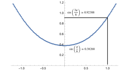
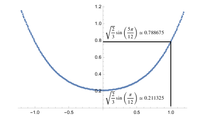
Figure 1: Graph of $|Z_{S^{3}_{b}}(b^{2}=1,M=0,\nu)|$ for $\widetilde{{\cal T}}_{(2,8)}$ theory (Left) and for $\widetilde{{\cal T}}_{(2,12)}$ theory (Right). The $|Z_{S^{3}_{b}}(b^{2}=1,M=0,\nu)|$s are even functions in $\nu$ and minimized at $\nu=0$. The values of $|Z_{S^{3}_{b}}(b^{2}=1,M=0,\nu=\pm 1)|$ are identical to the $|S_{\alpha=0,\beta=0}=S_{(1,1),(1,1)}|$ of $SM(2,8)$ and $SM(2,12)$ respectively. The value of $|Z_{S^{3}_{b}}(b^{2}=1,M=0,\nu=0)|$ is identical to the $\textrm{min}_{\beta}|S_{\alpha=0,\beta}|$ of $SM(2,8)$ and $SM(2,12)$ respectively. We draw the graph using the Bethe-sum formula in (61) combined with (64).

Superconformal index

The superconformal index for the theory before the monopole superpotential deformation is

$$\begin{split}&{\cal I}_{\rm sci}^{(K,Q)}(q;\vec{\eta},\vec{\nu})\\ &=\sum_{\mathbf{m}\in\mathbb{Z}^{r}}\left(\prod_{a=1}^{r}\oint\frac{du_{a}}{2\pi iu_{a}}\right)\left(\prod_{a=1}^{r}{\cal I}_{\Delta}(Q_{a}m_{a},u_{a}^{Q_{a}})(\eta_{a}(-q^{1/2})^{\nu_{a}})^{m_{a}}\right)\left(\prod_{a,b=1}^{r}u_{a}^{K_{ab}m_{b}}\right)\;.\end{split}$$ (44)

Here ${\cal I}_{\Delta}(m,u)$ is the tetrahedron index introduced in Dimofte:2011py , which computes the generalized superconformal index Kapustin:2011jm of the ${\cal T}_{\Delta}$ theory. See appendix A for details. After the monopole operator superpotential deformation, the superconformal index for the $\widetilde{{\cal T}}_{(2,4r)}$ theory is

$${\cal I}_{\rm sci}(q;\eta,\nu)={\cal I}^{(K,Q)}_{\rm sci}\left(q;\vec{\eta},\vec{\nu}=(\nu-1)\vec{A}\right)|_{\eta_{a}\rightarrow\eta^{A_{a}}}\;.$$ (45)

Using the expression above, one can compute the index and find that

$$\begin{split}&r=2:\\ &1-q^{1/2}-\left(1+\eta+\frac{1}{\eta}\right)q-\left(2+\eta+\frac{1}{\eta}\right)q^{3/2}-\left(2+\eta+\frac{1}{\eta}\right)q^{2}-q^{5/2}\\ &+\left(\eta^{2}+\frac{1}{\eta^{2}}+\eta+\frac{1}{\eta}+1\right)q^{3}+\left(\eta^{2}+\frac{1}{\eta^{2}}+2\eta+\frac{2}{\eta}+2\right)q^{7/2}+\ldots\\ &r=3:\\ &1-q^{1/2}-\left(1+\eta+\frac{1}{\eta}\right)q-\left(2+\eta+\frac{1}{\eta}\right)q^{3/2}-q^{2}+\left(\eta^{2}+\frac{1}{\eta^{2}}+2\eta+\frac{2}{\eta}+2\right)q^{5/2}\\ &+\left(2\eta^{2}+\frac{2}{\eta^{2}}+4\eta+\frac{4}{\eta}+6\right)q^{3}+\left(2\eta^{2}+\frac{2}{\eta^{2}}+6\eta+\frac{6}{\eta}+8\right)q^{7/2}+\ldots\\ &\textrm{for all $r\geq 2$}:\\ &{\cal I}_{\rm sci}(q;\eta,\nu=0)=1-q^{1/2}-\left(1+\eta+\frac{1}{\eta}\right)q-\left(2+\eta+\frac{1}{\eta}\right)q^{3/2}+\ldots\;,\end{split}$$ (46)

The index computation gives non-trivial evidences for the SUSY enhancement, ${\cal N}=2\rightarrow{\cal N}=5$, in the IR. First, only $q^{\mathbb{Z}/4}$-terms (actually only $q^{\mathbb{Z}/2}$) appear in the index which is compatible with the fact that $\frac{R_{\nu=0}}{2}+j_{3}\in\frac{\mathbb{Z}}{4}$ for any ${\cal N}\geq 3$ theory. This is quite non-trivial fact since the superconformal R-charge $R_{\nu=0}$ is determined by extremizing the function $F(\nu)=\log|{\cal Z}_{S^{3}_{b}}(b^{2}=1,M=0,\nu)|$, which is highly non-trivial function as drawn in Figure 1. Second, the index contains contributions from ${\cal N}=5$ stress-energy tensor multiplet. The ${\cal N}=5$ multiplet can be decomposed into several superconformal multiplets of a ${\cal N}=2$ subalgebra (which can be identified as the UV supersymmetry). They include Cordova:2016emh

$$\begin{split}&a)\;\textrm{Chiral primary multiplet with $\Delta=1$ in $\mathbf{1}$ of $SO(3)$}\;,\\ &b)\;\textrm{Conserved current multiplet in $\mathbf{3}$ of $SO(3)$}\;,\\ &c)\;\textrm{Extra-SUSY current multiplet in $\mathbf{3}$ of $SO(3)$}\;,\end{split}$$ (47)

where $SO(3)$ is the $SO(3)$ in $SO(2)\times SO(3)\subset SO(5)$ R-symmetry which is flavor symmetry in terms of the UV ${\cal N}=2$ supersymmetry. The ${\cal N}=2$ multiplets contribute to the index as follows

$$\begin{split}&a)\Rightarrow-q^{1/2}-q^{3/2}+\ldots\;,\\ &b)\Rightarrow-\left(1+\eta+\frac{1}{\eta}\right)q+\ldots\;,\\ &c)\Rightarrow-\left(1+\eta+\frac{1}{\eta}\right)q^{3/2}+\ldots\;,\end{split}$$ (48)

which can be obtained from the explicit multiplet structure in Cordova:2016emh . One can see that all these terms appear in the superconformal index. Even though the appearance do not guarantee the SUSY enhancement Evtikhiev:2017heo , since other ${\cal N}=2$ multiplets could give the same contributions, it provides non-trivial circumstantial evidence. As another non-trivial evidence, we will propose dual description in section 2.2.3 which has manifest ${\cal N}=5$ supersymmetry. For all $r\geq 2$, the indices in the A- and B-twisting limits become trivial, i.e.

$${\cal I}_{\rm sci}(\eta=1,\nu=\pm 1)=1\;.$$ (49)

It implies that the IR SCFT is of rank 0, if the SUSY enhancement really occurs, since the index in the A/B twisting limits compute the Coulomb/Higgs branch Hilbert-series Razamat:2014pta .

Twisted partition functions

To compute the twisted partition function, we first consider the integrand ${\cal I}^{(K,Q)}_{\hbar}$ of the squashed 3-sphere partition function (35) in the limit of $\hbar\rightarrow 0$ using (116):

$$\begin{split}&\log{\cal I}^{(K,Q)}_{\hbar}(\vec{Z};\vec{M},\vec{\nu})\xrightarrow{\quad\hbar\rightarrow 0\quad}\frac{1}{\hbar}{\cal W}_{0}^{(K,Q)}(\vec{Z};\vec{M},\vec{\nu})+{\cal W}_{1}^{(K,Q)}(\vec{Z};\vec{M},\vec{\nu})+O(\hbar)\\ &\textrm{ with }\\ &{\cal W}^{(K,Q)}_{0}=\sum_{a}{\rm Li}_{2}(e^{-Q_{a}Z_{a}})+\frac{1}{2}\vec{Z}\cdot K\cdot\vec{Z}+(\vec{M}+i\pi\vec{\nu})\cdot\vec{Z}\;,\\ &{\cal W}^{(K,Q)}_{1}=-\frac{1}{2}\sum_{a}\log(1-e^{-Q_{a}Z_{a}})+\frac{1}{2}\vec{Z}\cdot\vec{\nu}\;.\end{split}$$ (50)

Then, the twisted partition function can be computed as

$$\mathcal{Z}^{(K,Q)}_{{\cal M}_{g,p\in 2\mathbb{Z}}}(\vec{M},\vec{\nu})=\sum_{\vec{z}\in{\cal S}_{\rm BE}(\vec{M},\vec{\nu})}{\cal H}(\vec{z};\vec{M},\vec{\nu})^{g-1}({\cal F}(\vec{z};\vec{M},\vec{\nu}))^{p}\;,$$ (51)

where the Bethe-vacua ${\cal S}_{\rm BE}$ is the set of solutions of following algebraic equations ($\partial_{a}:=\partial_{Z_{a}}$)

$$\begin{split}&{\cal S}_{\rm BE}(\vec{M},\vec{\nu})=\bigg{\{}\vec{z}=(z_{1},\ldots,z_{r})\;:\;P_{a}(\vec{z};\vec{M},\vec{\nu})=1\textrm{ for all }a=1,\ldots,r\bigg{\}}\;,\\ &\textrm{ where }P_{a}:=\exp\left(\partial_{a}\mathcal{W}^{(K,Q)}_{0}\right)|_{\vec{Z}\rightarrow\log\vec{z}}=\left(\prod_{b=1}^{r}z_{b}^{K_{ab}}\right)(1-z_{a}^{-Q_{a}})^{Q_{a}}e^{M_{a}+i\pi\nu_{a}}\;.\end{split}$$ (52)

The handle-gluing and fibering operators are

$$\begin{split}&{\cal H}(\vec{z};\vec{M},\vec{\nu})=\left(\det_{a,b}\partial_{a}\partial_{b}{\cal W}_{0}\right)\exp\left(-2{\cal W}_{1}\right)\bigg{|}_{\vec{Z}\rightarrow\log\vec{z}}\;,\\ &{\cal F}(\vec{z};\vec{M},\vec{\nu})=\exp\left(-\frac{{\cal W}_{0}-\vec{Z}\cdot\partial_{\vec{Z}}{\cal W}_{0}-\vec{M}\cdot\partial_{\vec{M}}{\cal W}_{0}}{2\pi i}\right)\bigg{|}_{\vec{Z}\rightarrow\log\vec{z}}\;.\end{split}$$ (53)

Then, twisted partition functions for the $\widetilde{{\cal T}}_{(2,4r)}$ theory is given as

$$\begin{split}&\mathcal{Z}_{{\cal M}_{g,p\in 2\mathbb{Z}}}(M,\nu)=\sum_{\vec{z}_{\alpha}\in{\cal S}_{\rm BE}}{\cal H}(\vec{z}_{\alpha};M,\nu)^{g-1}{\cal F}(\vec{z}_{\alpha};M,\nu)^{p}\;,\\ &\textrm{with }{\cal H}/{\cal F}(\vec{z}_{\alpha};M,\nu):={\cal H}/{\cal F}(\vec{z}_{\alpha};\vec{M}=\vec{A}M,\vec{\nu}=(\nu-1)\vec{A})\;.\end{split}$$ (54)

There are two distinct SUSY backgrounds on ${\cal M}_{g,p\in 2\mathbb{Z}}$ depending on the spin-structure choices along the fiber $[S^{1}]$-direction Closset:2018ghr . In the above computation, we choose an anti-periodic, which corresponds to $\nu_{R}=\frac{1}{2}(\textrm{mod 1})$ in Closset:2018ghr . Due to the phase ambiguity of squashed 3-sphere partition function in (43), the ${\cal F}(\vec{z}_{\alpha})$ and ${\cal H}(\vec{z}_{\alpha})$ have $\alpha$-independent phase factor ambiguities. For rank-0 SCFTs, one can fix the overall phase factor ambiguity of ${\cal H}(\vec{z}_{\alpha})$ by requiring that

$${\cal H}(\vec{z}_{\alpha};M=0,\nu=\pm 1)\in\mathbb{R}_{>0}\textrm{ for all }\vec{z}_{\alpha}\in{\cal S}_{\rm BE}\;.$$ (55)

This is possible since all the ${\cal H}(\vec{z}_{\alpha};M=0,\nu=\pm 1)$ have the same phase for rank-0 SCFTs.

For the $\widetilde{{\cal T}}_{(2,4r)}$ theory, there are $r$ Bethe-vacua, $\{\vec{z}_{\alpha}\}_{\alpha=0}^{r-1}$, and their handle-gluing/fibering operators in the A-twisting limit, $M\rightarrow 0$ and $\nu\rightarrow-1$, are

$$\begin{split}&{\cal H}(\vec{z}_{\alpha};M=0,\nu=-1)=(S_{(1,1),(1,2\alpha+1)})^{-2}\;,\\ &{\cal F}(\vec{z}_{\alpha};M=0,\nu=-1)^{2}=e^{2\pi i\delta}\exp\left(4\pi ih_{(s=1,t=2\alpha+1)}\right)\;.\end{split}$$ (56)

with a $\delta\in\mathbb{Q}$. Here $S$ and $h_{(s,t)}$ is the S-matrix (6) and conformal dimensions (3) of $SM(2,4r)$.

Let $L$ be the supersymmetric Wilson loop of gauge charge $\vec{\mathfrak{q}}=(\mathfrak{q}_{1},\ldots,\mathfrak{q}_{r})$. The twisted partition function with insertion of the loop operator can be computed as

$$\mathcal{Z}^{L}_{{\cal M}_{g,p\in 2\mathbb{Z}}}(M,\nu)=\sum_{\vec{z}_{\alpha}\in{\cal S}_{\rm BE}}{\cal H}(\vec{z}_{\alpha})^{g-1}{\cal F}(\vec{z}_{\alpha})^{p}L(\vec{z}_{\alpha})\;,$$ (57)

$$\textrm{with }L(\vec{z}):=\prod_{a=1}^{r}(z_{a})^{\mathfrak{q}_{a}}\;.$$ (58)

For the $\widetilde{{\cal T}}_{(2,4r)}$ theory, let $\{L_{\alpha}\}_{\alpha=0,1,\ldots,r-1}$ be supersymmetric Wilson loop operators with following gauge charge $\vec{\mathfrak{q}}_{\alpha}$:

$$\vec{\mathfrak{q}}_{\alpha}=(0,1,2,\ldots,\alpha-1,\alpha,\ldots,\alpha)\;.$$ (59)

Then, one can check that

$$W_{\beta}(\alpha):=L_{\alpha}(\vec{z}_{\beta})=\frac{S_{(1,2\alpha+1),(1,2\beta+1)}}{S_{(1,1),(1,2\beta+1)}}\;.$$ (60)

Using the handle-gluing and fibering operators, the round 3-sphere in (35) can be written in the following Bethe-sum Closset:2017zgf ; Gang:2019jut :

$$|{\cal Z}^{(K,Q)}_{S^{3}_{b=1}}(\vec{M},\vec{\nu})|=|\sum_{\vec{z}_{\alpha}\in{\cal S}_{\rm BE}}{\cal H}(\vec{z}_{\alpha};\vec{M},\vec{\nu})^{-1}{\cal F}(\vec{z}_{\alpha};\vec{M},\vec{\nu})|\;,$$ (61)

only when the $\vec{\nu}$ satisfies following conditions Gang:2019jut

$$K_{aa}+\nu_{a}\in 2\mathbb{Z}$$ (62)

For the $\widetilde{{\cal T}}_{(2,4r)}$ theory, the condition is met if

$$\nu_{1}\in 2\mathbb{Z}+1,\quad\nu_{a>1}\in 2\mathbb{Z}\;.$$ (63)

For general $\vec{\nu}$, the round 3-sphere partition function can be computed using the following relation

$${\cal Z}^{(K,Q)}_{S^{3}_{b=1}}(\vec{M},\vec{\nu})=|{\cal Z}^{(K,Q)}_{S^{3}_{b=1}}(\vec{M}+2\pi i(\vec{\nu}-\vec{\nu}_{0}),\vec{\nu}_{0})|\;,$$ (64)

with $\vec{\nu}_{0}$ is chosen to satisfy the condition in (62).

Half-indices

The half index of the $\widetilde{{\cal T}}_{(2,4r)}$ theory with $\mathbb{B}=({\cal D},D_{c})$ boundary condition is Dimofte:2017tpi

$$\begin{split}I_{\rm half}(q;\eta,\nu)&=I^{(K,Q)}_{\rm half}(q;\vec{\eta},\vec{\nu}=(\nu-1)\vec{A})\big{|}_{\eta_{a}\rightarrow\eta^{A_{a}}}\\ &=\sum_{\mathbf{m}\in(\mathbb{Z}_{\geq 0})^{r}}\frac{q^{\frac{1}{2}\mathbf{m}\cdot K\cdot\mathbf{m}}(\eta(-q^{1/2})^{(\nu-1)})^{-\vec{A}\cdot\mathbf{m}}}{(q)_{m_{1}}\ldots(q)_{m_{r}}}\;.\end{split}$$ (65)

where

$$\begin{split}I^{(K,Q)}_{\rm half}(q;\vec{\eta},\vec{\nu})&=\frac{1}{(q)^{r}_{\infty}}\sum_{\mathbf{m}\in\mathbb{Z}^{r}}q^{\frac{1}{2}\mathbf{m}\cdot K\cdot\mathbf{m}}\prod_{a=1}^{r}\left((\eta_{a}(-q^{1/2})^{\nu_{a}})^{m_{a}}(q^{1-Q_{a}m_{a}};q)_{\infty}\right)\\ &=\sum_{\mathbf{m}\in(\mathbb{Z}_{\geq 0})^{r}}\frac{q^{\frac{1}{2}\mathbf{m}\cdot K\cdot\mathbf{m}}\prod_{a=1}^{r}(\eta_{a}(-q^{1/2})^{\nu_{a}})^{-m_{a}}}{(q)_{Q_{1}m_{1}}\ldots(q)_{Q_{r}m_{r}}}\;.\end{split}$$ (66)

Here $\mathbb{B}=({\cal D},D_{c})$ is Dirichlet boundary condition (${\cal D}$) for vector multiplets and deformed Dirichlet boundary condition ($D_{c}$) for chiral multiplet. In terms of 2D (0,2) subalgebra, a 3D chiral multiplet is decomposed into a 2d chiral multiplet $\Phi_{2d}$ and a 2d Fermi multiplet. The deformed Dirichlet boundary condition $D_{c}$(or Dirichlet boundary condition $D$) is imposing $\Phi_{2d}=c$ (or $\Phi_{2d}=0$) with non-zero $c$. The boundary condition breaks all the $U(1)^{r}$ gauge symmetry while preserving the $U(1)$ R-symmetry. We assign zero R-charge to the chiral fields.

The half-index with the Wilson loop operator $L_{\alpha}$ in (59) becomes Dimofte:2017tpi

$$I^{L_{\alpha}}_{\rm half}(q;\eta,\nu)=\sum_{\mathbf{m}\in(\mathbb{Z}_{\geq 0})^{r}}\frac{q^{\frac{1}{2}\mathbf{m}\cdot K\cdot\mathbf{m}}(\eta(-q^{1/2})^{(\nu-1)})^{-\vec{A}\cdot\mathbf{m}}q^{-\vec{\mathfrak{q}}_{\alpha}\cdot\mathbf{m}}}{(q)_{m_{1}}\ldots(q)_{m_{r}}}$$ (67)

In the A-twisting limit, $\eta\rightarrow 1$ and $\nu\rightarrow-1$, the half-indices reproduce the characters of 2D RCFT $(SM(2,4r))\otimes(\textrm{free Fermion})$

$$\begin{split}&q^{h_{\alpha}-\frac{c}{24}}I^{L_{\alpha}}_{\rm half}(q;\eta=1,\nu=-1)=q^{h_{\alpha}-\frac{c}{24}}\sum_{\mathbf{m}\in(\mathbb{Z}_{\geq 0})^{r}}\frac{q^{\frac{1}{2}\mathbf{m}\cdot K\cdot\mathbf{m}+\vec{A}\cdot\mathbf{m}-\vec{\mathfrak{q}}_{\alpha}\cdot\mathbf{m}}}{(q)_{m_{1}}\ldots(q)_{m_{r}}}\\ &=\left(\chi_{s=1,t=2\alpha+1}(q)\textrm{ of $SM(2,4r)$ in \eqref{SM-characters}}\right)\times\chi_{F}(q)\;,\end{split}$$ (68)

up to an overall factor $q^{h_{\alpha}-\frac{c}{24}}$ where

$$c=8-\frac{3}{2r}-6r\;,\quad h_{\alpha}=\frac{\alpha(1-2r+\alpha)}{4r}\;.$$ (69)

The $c$ is the central charge of the product RCFT, $\left(c\textrm{ in \eqref{c and h} for $SM(2,4r)$}\right)+\frac{1}{2}$, and $h_{\alpha}$ is the conformal dimension of $SM(2,4r)$. It provides a novel fermionic sum expression for the product RCFT characters. In the above, $\chi_{F}(q)$ is the character of 2D free Majorana-Weyl fermion theory, whose bulk 3D TQFT is the Ising spin-TQFT $SO(1)_{1}$,

$$\chi_{F}(q)=q^{-\frac{1}{48}}\mathbb{I}_{D}(x=-q^{1/2};q)=q^{-\frac{1}{48}}\prod_{n=0}^{\infty}(1+q^{n+1/2})=q^{-\frac{1}{48}}(-q^{1/2};q)_{\infty}\;.$$ (70)

We define

$$\mathbb{I}_{D}(x;q):=(x^{-1}q;q)_{\infty}=\prod_{n=0}^{\infty}(1-q^{n+1}x^{-1})\;,$$ (71)

which is the half-index for the ${\cal T}_{\Delta}$ theory in the Dirichlet boundary ($D$) and with $R(\Phi)=0$. For general R-charge, the half index for ${\cal T}_{\Delta}$ is $\mathbb{I}_{D}(x(-q^{1/2})^{R(\Phi)};q)$.

The equations in (56),(60),(68) and the Figure 1 give non-trivial evidences for the proposal in (22) for the $\widetilde{{\cal T}}_{(2,4r)}$. They are all compatible with the bulk-boundary dictionaries listed in Table 1.

2.2.2 UV description II

The 2nd UV gauge theory description is (for $r=2,4,6,\ldots$)

$$\begin{split}&{\cal T}_{(2,2r+4)}:=\frac{({\cal T}_{\Delta})^{\otimes r}}{[U(1)^{r}_{\mathbf{Q}}]_{K}}\textrm{ with superpotential }{\cal W}={\cal O}_{(\mathbf{m}_{1},\mathbf{n}_{1})}+\ldots+{\cal O}_{(\mathbf{m}_{r-1},\mathbf{n}_{r-1})}\\ &K=C(T_{r})^{-1}:=\begin{pmatrix}1&1&1&\cdots&1&1\\ 1&2&2&\cdots&2&2\\ 1&2&3&\cdots&3&3\\ \vdots&\vdots&\vdots&\ddots&\vdots&\vdots\\ 1&2&3&\cdots&r-1&r-1\\ 1&2&3&\cdots&r-1&r\end{pmatrix},\quad\mathbf{Q}=\mathbb{I}_{r\times r},\\ &\mathbf{m}_{1}=(1,1,-1,\mathbf{0}_{r-3}),\;\mathbf{m}_{2\leq I\leq r-2}=(\mathbf{0}_{I-2},-1,1,1,-1,\mathbf{0}_{r-I-2}),\;\mathbf{m}_{r-1}=(\mathbf{0}_{r-2},-2,2),\\ &\mathbf{n}_{1\leq I\leq r-1}=(\mathbf{0}_{r})\;.\end{split}$$ (72)

Here the $C(T_{r})$ is the Cartan matrix of the tadpole graph, obtained by folding the Cartan matrix of $A_{r}$ in half. The ${\cal N}=2$ gauge theory has a $U(1)$ flavor symmetry, $U(1)_{A}$, whose charge is given as

$$A=\vec{A}\cdot\vec{T}=\sum_{a=1}^{r}\left[\frac{a+1}{2}\right]T_{a}=T_{1}+T_{2}+2T_{3}+2T_{4}+\ldots+\frac{r}{2}T_{r-1}+\frac{r}{2}T_{r}\;.$$ (73)

In the above equation square brackets mean integer part. Solving the constraints in (38), the $(\vec{M},\vec{\nu})$ can be parameterized as

$$\vec{M}=\vec{A}M\;,\quad\vec{\nu}=(\nu-1)\vec{A}\;.$$ (74)

The bulk supersymmetric partition functions of the gauge theory can be computed as

$$\begin{split}&{\cal Z}_{S^{3}_{b}}(b^{2},M,\nu)={\cal Z}^{(K,Q)}_{S^{3}_{b}}(\vec{M}=\vec{A}M,\vec{\nu}=(\nu-1)\vec{A})\;,\\ &{\cal I}_{\rm sci}(q;\eta,\nu)={\cal I}^{(K,Q)}_{\rm sci}\left(q;\vec{\eta},\vec{\nu}=(\nu-1)\vec{A}\right)\bigg{|}_{\eta_{a}\rightarrow\eta^{A_{a}}}\;,\\ &{\cal Z}_{{\cal M}_{g,p\in 2\mathbb{Z}}}(M,\nu)={\cal Z}^{(K,Q)}_{{\cal M}_{g,p\in 2\mathbb{Z}}}(\vec{M}=\vec{A}M,\vec{\nu}=(\nu-1)\vec{A})\;.\end{split}$$ (75)

where the ${\cal Z}_{S^{3}_{b}}^{(K,Q)},{\cal I}_{\rm sci}^{(K,Q)}$ and ${\cal Z}_{{\cal M}_{g,p\in 2\mathbb{Z}}}$ are given in (35), (44) and (51) respectively. Superconformal R-charge can be determined by F-maximization, in the same way as (42) and one can confirm that the $\nu=0$ in the parametrization (74) corresponds to the superconformal R-charge. Numerically, one can check that

$$\left({\cal Z}_{S^{3}_{b}}(b^{2}=1,M,\nu)\textrm{ of }{\cal T}_{(2,2r+4)}\right)=\left({\cal Z}_{S^{3}_{b}}(b^{2}=1,M,\nu)\textrm{ of }\widetilde{T}_{(2,2r+4)}\textrm{ in \eqref{UV theory for (2,4r)-I}}\right)\;.$$ (76)

For the superconformal index we find that, for all $r\in 2\mathbb{Z}_{\geq 1}$

$$\begin{split}&{\cal I}_{\rm sci}(q;\eta,\nu=0)=1-q^{1/2}-\left(1+\eta+\frac{1}{\eta}\right)q-\left(2+\eta+\frac{1}{\eta}\right)q^{3/2}+\ldots\;,\\ &{\cal I}_{\rm sci}(\eta=1,\nu=\pm 1)=1\;,\\ &\left({\cal I}_{\rm sci}(\eta=1,\nu=\pm 1)\textrm{ of ${\cal T}_{(2,2r+4)}$}\right)=\left({\cal I}_{\rm sci}(\eta=1,\nu=\pm 1)\textrm{ of $\widetilde{{\cal T}}_{(2,2r+4)}$ in \eqref{UV theory for (2,4r)-I}}\right)\;.\end{split}$$ (77)

As argued for the $\widetilde{{\cal T}}_{(2,2r+4)}$ case, the superconformal index give non-trivial evidences for the SUSY enhancement, ${\cal N}=2\rightarrow{\cal N}=5$, in the IR.

In the twisted partition computation, there are $(\frac{r}{2}+1)$ Bethe-vacua, $\{\vec{z}_{\alpha}\}_{\alpha=0}^{\frac{r}{2}}$, and their handle-gluing/fibering operators in the A-twisting limit, $\vec{M}\rightarrow\vec{0}$ and $\vec{\nu}\rightarrow-2\vec{A}$, are

$$\begin{split}&{\cal H}(\vec{z}_{\alpha};\vec{M}=0,\vec{\nu}=-2\vec{A})=(S_{(1,1),(1,2\alpha+1)})^{-2}\;,\\ &\left({\cal F}(\vec{z}_{\alpha};\vec{M}=0,\vec{\nu}=-2\vec{A})\right)^{2}=e^{2\pi i\delta}\exp\left(4\pi ih_{(s=1,t=2\alpha+1)}\right)\;,\end{split}$$ (78)

with a $\delta\in\mathbb{Q}$. Here $S$ and $h_{(s,t)}$ is the S-matrix (6) and conformal dimensions (3) of $SM(2,2r+4)$.

The half-index for the ${\cal T}_{(2,2r+4)}$ theory is

$$\begin{split}I_{\rm half}(q;\eta,\nu)&=I^{(K,Q)}_{\rm half}(q;\vec{\eta},\vec{\nu}=(\nu-1)\vec{A})\big{|}_{\eta_{a}\rightarrow\eta^{A_{a}}}\\ &=\sum_{\mathbf{m}\in(\mathbb{Z}_{\geq 0})^{r}}\frac{q^{\frac{1}{2}\mathbf{m}\cdot K\cdot\mathbf{m}}(\eta(-q^{1/2})^{(\nu-1)})^{-\vec{A}\cdot\mathbf{m}}}{(q)_{\mathbf{m}_{1}}\ldots(q)_{\mathbf{m}_{r}}}\;.\end{split}$$ (79)

Let $\{L_{\alpha}\}_{\alpha=0,1,\ldots,\frac{r}{2}}$ be supersymmetric Wilson loop operators with gauge charge $\vec{\mathfrak{q}}_{\alpha}$:

$$\vec{\mathfrak{q}}_{\alpha}=(1,1,2,2,\ldots,\alpha-1,\alpha-1,\alpha,\alpha,\alpha,\ldots,\alpha)\;.$$ (80)

The half-index with the loop operator $L_{\alpha}$ becomes

$$I^{L_{\alpha}}_{\rm half}(q;\eta,\nu)=\sum_{\mathbf{m}\in(\mathbb{Z}_{\geq 0})^{r}}\frac{q^{\frac{1}{2}\mathbf{m}\cdot K\cdot\mathbf{m}}(\eta(-q^{1/2})^{(\nu-1)})^{-\vec{A}\cdot\mathbf{m}}q^{-\vec{\mathfrak{q}}_{\alpha}\cdot\mathbf{m}}}{(q)_{m_{1}}\ldots(q)_{m_{r}}}\;.$$ (81)

In the A-twisting limit, $\eta\rightarrow 1$ and $\nu\rightarrow-1$, the half-indices reproduce the characters of 2D RCFT $SM(2,2r+4)$

$$\begin{split}&q^{h_{\alpha}-\frac{c}{24}}I^{L_{\alpha}}_{\rm half}(q;\eta=1,\nu=-1)=q^{h_{\alpha}-\frac{c}{24}}\sum_{\mathbf{m}\in(\mathbb{Z}_{\geq 0})^{r}}\frac{q^{\frac{1}{2}\mathbf{m}\cdot K\cdot\mathbf{m}+\vec{A}\cdot\mathbf{m}-\vec{\mathfrak{q}}_{\alpha}\cdot\mathbf{m}}}{(q)_{m_{1}}\ldots(q)_{m_{r}}}\\ &=\left(\chi_{(s=1,t=2\alpha+1)}(q)\textrm{ of $SM(2,2r+4)$ in \eqref{SM-characters}}\right)\;.\end{split}$$ (82)

Here $K$ and $A$ are given in (72) and (73), and the $c$ and $h_{\alpha}$ are the central charge and the conformal dimension of $SM(2,2r+4)$ as given in (3). The half-indices in (82) reproduce the known fermionic sum expression for the characters of $SM(2,2r+4)$ in Melzer:1994qp .

The nice matches in (78) and (82) support the proposal in (22) for the ${\cal T}_{(2,4r)}$ case.

2.2.3 UV description III

The 3rd UV description is

$$\begin{split}&\widetilde{{\cal T}}^{\prime}_{(2,4r)}:=SU(2)_{k=r}^{\frac{1}{2}\oplus\frac{1}{2}}\\ &:=\textrm{ $SU(2)$ gauge theory coupled to a half hypermultiplet and a half twisted}\\ &\quad\;\;\textrm{-hypermultiplet in the fundamental representations with Chern-Simons level $k=r$.}\end{split}$$ (83)

The theory is a rank-0 ${\cal N}=4$ SCFT and actually has ${\cal N}=5$ supersymmetry Hosomichi:2008jb ; Gang:2021hrd .

Chiral multiplet	$SU(2)$	$R_{\nu=0}$	$A$
$\Phi_{1}$	$\mathbf{2}$	$\frac{1}{2}$	$+\frac{1}{2}$
$\Phi_{2}$	$\mathbf{2}$	$\frac{1}{2}$	$-\frac{1}{2}$

Table 2: Matter contents of $SU(2)_{k}^{\frac{1}{2}\oplus\frac{1}{2}}$ theory in terms of ${\cal N}=2$ chiral multiplets. $SU(2)$, $R_{\nu=0}$ and $A$ represent $SU(2)$ gauge symmetry, superconformal R-charge and charge of $U(1)_{A}$ symmetry respectively. The theory has a superpotential term ${\cal W}\propto\frac{1}{k}(\epsilon_{ij}\Phi^{i}_{1}\Phi^{j}_{2})^{2}$ where $i$ and $j=1,2$ are indices for $\mathbf{2}$ of $SU(2)$ gauge group.

Squashed 3-sphere partition function

The partition function is given as

$$\begin{split}{\cal Z}_{S^{3}_{b}}(M,\nu)&=\int\frac{dZ}{\sqrt{2\pi\hbar}}{\cal I}_{\hbar}(Z,M,\nu)\textrm{ with}\\ {\cal I}_{\hbar}(Z,M,\nu)&=2\sinh(Z)\sinh(\frac{2\pi iZ}{\hbar})\exp\left(\frac{(r+1)Z^{2}}{\hbar}\right)\\ &\times\prod_{\epsilon_{1},\epsilon_{2}\in\{\pm 1\}}\psi_{\hbar}\left(\epsilon_{1}Z+\epsilon_{2}\frac{M+\nu(i\pi+\hbar/2)}{2}+\frac{(i\pi+\hbar/2)}{2}\right)\;.\end{split}$$ (84)

Here $(M,\nu)$ is the (rescaled real mass, R-symmetry mixing parameter) for the $U(1)_{A}$ symmetry.

Superconformal index

The superconformal index is

$$\begin{split}{\cal I}_{\rm sci}(q;\eta,\nu)=&\sum_{m\in\mathbb{Z}_{\geq 0}}\oint_{|u|=1}\frac{du}{2\pi iu}\Delta(m,u)u^{2(r+1)m}{\cal I}_{\Delta}\left(m,u(\eta q)^{1/2}\right)\\ &\times{\cal I}_{\Delta}\left(-m,u^{-1}(\eta q)^{1/2}\right){\cal I}_{\Delta}\left(m,u\eta^{-1/2}\right){\cal I}_{\Delta}\left(-m,u^{-1}\eta^{-1/2}\right)\big{|}_{\eta\rightarrow\eta(-q^{1/2})^{\nu-1}}\;.\end{split}$$ (85)

Here $\Delta(m,u)$ is the contribution from the $SU(2)$ vector multiplet

$$\begin{split}&\Delta(m,u)=\frac{1}{{\rm Sym}(m)}(q^{\frac{m}{2}}u-q^{-\frac{m}{2}}u^{-1})(q^{\frac{m}{2}}u^{-1}-q^{-\frac{m}{2}}u)\;,\\ &\textrm{where }\textrm{Sym}(m):=\begin{cases}2,\quad m=0\\ 1,\quad m>0\;.\end{cases}\end{split}$$ (86)

One can check that the index matches with the superconformal index (45) computed using the UV gauge theory in (24).

Twisted partition functions

In the asymptotic $\hbar\rightarrow 0$ limit, the integrand of squashed 3-sphere partition function behaves as (in the limit $\nu\rightarrow-1$)

$$\begin{split}&\log{\cal I}_{\hbar}(Z,M,\nu)\xrightarrow{\quad\hbar\rightarrow 0\quad}\frac{1}{\hbar}{\cal W}_{0}(Z;M,\nu)+{\cal W}_{1}(Z;M,\nu)\;,\\ &{\cal W}_{0}=\pm 2\pi iZ+(r+1)Z^{2}+\sum_{\epsilon_{2},\epsilon_{2}\in\{\pm 1\}}{\rm Li}_{2}(\epsilon_{2}e^{-\epsilon_{1}Z-\epsilon_{2}\frac{M}{2}})\;,\\ &{\cal W}_{1}=-\frac{1}{2}\log(1-e^{-Z-\frac{M}{2}})-\frac{1}{2}\log(1-e^{Z-\frac{M}{2}})+\log(\sinh Z)\;.\end{split}$$ (87)

The corresponding Bethe equation is

$$P(z;M,\nu=-1)=\exp(\partial_{Z}W_{0})|_{Z\rightarrow\log z}=\frac{z^{2r}\left(e^{M/2}+z\right)\left(e^{M/2}z-1\right)}{\left(e^{M/2}-z\right)\left(e^{M/2}z+1\right)}=1\;.$$ (88)

In the A-twisting limit, $(M,\nu)=(0,-1)$, the $P(z)=-z^{2r}$ and there are $r$ Bethe-vacua

$$\begin{split}&{\cal S}_{\rm BE}(M=0,\nu=-1)=\{z\;:\;P(z,M=0,\nu=-1)=1\textrm{ and }z^{2}\neq 1\}/\mathbb{Z}_{2}\\ &=\bigg{\{}z_{\alpha}=\exp\left(\frac{i\pi(2\alpha+1)}{2r}\right):\alpha=0,\ldots,r-1\bigg{\}}\;,\end{split}$$ (89)

taking into account the quotient by the Weyl symmetry $\mathbb{Z}_{2}$, $z\rightarrow 1/z$. The corresponding handle-gluing operator ${\cal H}$ is

$$\begin{split}&{\cal H}(z;M=0,\nu=-1)=-\frac{1}{4}(\partial_{Z}\partial_{Z}{\cal W}_{0})e^{-2{\cal W}_{1}}\bigg{|}_{Z\rightarrow\log z}=\frac{2rz}{4(z+1)^{2}}\;,\\ &\Rightarrow{\cal H}(z_{\alpha})=\frac{r}{2}\cos\left(\frac{(2\alpha+1)\pi)}{4r}\right)^{-2}=(S_{(1,1),(1,2\alpha+1)})^{-2}\;.\end{split}$$ (90)

The factor $1/4$ comes from $1/|W(G)|^{2}$ Gang:2021hrd and the $(-1)$ is to fix the overall phase factor of ${\cal H}$ according to (55). The corresponding fibering-gluing operator ${\cal F}$ is

$$\begin{split}&{\cal F}(z;M,\nu)=\exp\left(-\frac{{\cal W}_{0}-Z\partial_{Z}W_{0}-M\partial_{M}W_{0}}{2\pi i}\right)\bigg{|}_{Z\rightarrow\log z}\;.\end{split}$$ (91)

Using the expression, one can confirm that

$$|{\cal F}(z_{\alpha};M=0,\nu=-1)|=1\textrm{ and }\left(\frac{{\cal F}(z_{\alpha};M=0,\nu=-1)}{{\cal F}(z_{\alpha=0};M=0,\nu=-1)}\right)^{2}=\exp(4\pi ih_{(1,2\alpha+1)})\;.$$ (92)

Half-indices

The half index for the $SU(2)_{k=r}^{\frac{1}{2}\oplus\frac{1}{2}}$ theory is

$$\begin{split}&I_{\rm half:\mathbb{B}}(q;\eta,\nu)=\textrm{Tr}_{{\cal H}(HS^{2}:\mathbb{B})}(-1)^{R_{\nu}}q^{R_{\nu}+j_{3}}x^{2J_{3}}\eta^{A+J_{3}}\big{|}_{x\rightarrow 1}\\ &=\sum_{m\in\mathbb{Z}}\frac{q^{(r-1)m^{2}}x^{2(r-1)m}\eta^{(r-1)m}}{(q;q)_{\infty}(q^{1+2m}x^{2}\eta;q)_{\infty}(q^{1-2m}x^{-2}\eta^{-1};q)_{\infty}}\\ &\times\mathbb{I}_{D}\left(-q^{m+1/2}x\eta;q\right)\mathbb{I}_{D}\left(-q^{-m+1/2}x^{-1};q\right)\mathbb{I}_{D}\left(q^{m}x;q\right)\mathbb{I}_{D}\left(q^{-m}(x\eta)^{-1};q\right)\bigg{|}_{\eta\rightarrow\eta(-q^{1/2})^{\nu-1},x\rightarrow 1}\;.\end{split}$$ (93)

The half index agrees with the half index of the $\widetilde{{\cal T}}_{(2,4r)}$ theory in (24):

$$\left(I_{\rm half}(q;\eta,\nu)\textrm{ in \eqref{half-index (2,4r)-2}}\right)=\left(I_{\rm half}(q;\eta,\nu)\textrm{ in \eqref{half-index (2,4r)}}\right)\;.$$ (94)

In the A-twisting limit, $\eta\rightarrow 1$ and $\nu\rightarrow-1$, the half-index is related to the vacuum character of $SM(2,4r)$ as follows

$$q^{-\frac{c}{24}}I_{\rm half:\mathbb{B}}(q;\eta=1,\nu=-1)=\left(\chi_{(1,1)}(q)\textrm{ of $SM(2,4r)$ in \eqref{SM-characters}}\right)\times\left(\chi_{F}(q)\textrm{ in \eqref{free-fermion character}}\right)\;,$$ (95)

where $c$ is given in (69). In the limit, we impose the Dirichlet boundary condition for $SU(2)$ vector multiplet. We assign R-charge $R=(-1,1,0,2)$ to the 4 ($\mathbf{2}+\mathbf{2}$) chiral multiplets and impose Dirichlet boundary condition for the 3 chirals with $R\neq 0$ and deformed Dirichlet boundary condition for the chiral with $R=0$. The R-charge assignment and boundary condition break the $SU(2)$ gauge symmetry while preserving the R-symmetry.

The nice matches in (90),(92) and (95) support the proposal in (22) for the $\widetilde{{\cal T}}^{\prime}_{(2,4r)}$.

2.3 Bulk dual rank-0 SCFT of $SM(3,6r-5)$

In the following we propose UV gauge theory description of $\mathcal{T}_{(3,6r-5)}$ modulo a decoupled Ising spin-TQFT, $SO(1)_{1}$:

$$\left(\widetilde{{\cal T}}_{(3,6r-5)}\textrm{ in \eqref{UV theory for (3,6r-5)}}\right)\xrightarrow{\;\textrm{A-twisting/bulk-boundary}\;}SM(3,6r-5)\otimes(\textrm{Free fermion}).$$ (96)

2.3.1 UV description

The UV gauge theory description is ($r\geq 2$),

$$\begin{split}&\widetilde{{\cal T}}_{(3,6r-5)}:=\frac{({\cal T}_{\Delta})^{\otimes r}}{[U(1)^{r}_{\mathbf{Q}}]_{K}}\textrm{ with superpotential }{\cal W}={\cal O}_{(\mathbf{m}_{1},\mathbf{n}_{1})}+\ldots+{\cal O}_{(\mathbf{m}_{r-1},\mathbf{n}_{r-1})}\\ &K=\begin{pmatrix}1&-1&-1&\cdots&-1&-1\\ -1&2&2&\cdots&2&2\\ -1&2&4&\cdots&4&4\\ \vdots&\vdots&\vdots&\ddots&\vdots&\vdots\\ -1&2&4&\cdots&2(r-2)&2(r-2)\\ -1&2&4&\cdots&2(r-2)&2(r-1)\end{pmatrix},\quad\mathbf{Q}=\textrm{diag}\{\mathbf{1}_{r-1},2\}\;,\\ &\mathbf{m}_{1}=(2,\mathbf{0}_{r-1}),\;\mathbf{m}_{2}=(0,2,-1,\mathbf{0}_{r-3}),\;\mathbf{m}_{3\leq I\leq r-1}=(\mathbf{0}_{I-2},-1,2,-1,\mathbf{0}_{r-I-1})\;,\\ &\mathbf{n}_{1}=(0,\mathbf{2}_{r-2},1),\;\mathbf{n}_{2}=(1,\mathbf{0}_{r-1}),\;\mathbf{n}_{3\leq I\leq r-1}=(\mathbf{0}_{r})\;.\end{split}$$ (97)

The ${\cal N}=2$ gauge theory has a $U(1)$ flavor symmetry, $U(1)_{A}$, whose charge is given as

$$A=\vec{A}\cdot\vec{T}=\sum_{a=1}(a-1)T_{a}=T_{2}+2T_{3}+\ldots+(r-1)T_{r}\;.$$ (98)

Solving the constraints in (38), the $(\vec{M},\vec{\nu})$ can be parameterized as

$$\vec{M}=\vec{A}M\;,\quad\vec{\nu}=(\nu-1)\vec{A}\;.$$ (99)

The bulk supersymmetric partition functions of the gauge theory can be computed as

$$\begin{split}&{\cal Z}_{S^{3}_{b}}(b^{2},M,\nu)={\cal Z}^{(K,Q)}_{S^{3}_{b}}(\vec{M}=\vec{A}M,\vec{\nu}=(\nu-1)\vec{A})\;,\\ &{\cal I}_{\rm sci}(q;\eta,\nu)={\cal I}^{(K,Q)}_{\rm sci}\left(q;\vec{\eta},\vec{\nu}=(\nu-1)\vec{A}\right)\bigg{|}_{\eta_{a}\rightarrow\eta^{A_{a}}}\;,\\ &{\cal Z}_{{\cal M}_{g,p\in 2\mathbb{Z}}}(M,\nu)={\cal Z}^{(K,Q)}_{{\cal M}_{g,p\in 2\mathbb{Z}}}(\vec{M}=\vec{A}M,\vec{\nu}=(\nu-1)\vec{A})\;.\end{split}$$ (100)

where the ${\cal Z}_{S^{3}_{b}}^{(K,Q)},{\cal I}_{\rm sci}^{(K,Q)}$ and ${\cal Z}_{{\cal M}_{g,p\in 2\mathbb{Z}}}$ are given in (35), (44) and (51) respectively. Superconformal R-charge can be determined by F-maximization, in the same way as (42).

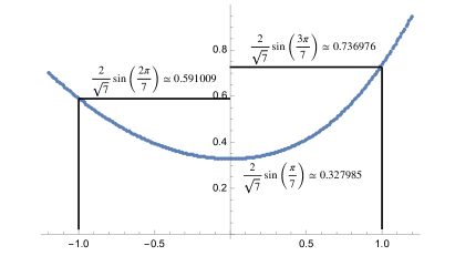
Figure 2: Graph of $|Z_{S^{3}_{b}}(b^{2}=1,M=0,\nu)|$ for $\widetilde{{\cal T}}_{(3,7)}$ theory (Left) and for $\widetilde{{\cal T}}_{(3,13)}$ theory (Right). For both cases, the round 3-sphere partition functions are minimized at $\nu=0$. The values of $|Z_{S^{3}_{b}}(b^{2}=1,M=0,\nu=-1)|$ are identical to the $|S_{\alpha=0,\beta=0}=S_{(1,1),(1,1)}|$ of $SM(3,7)$ and $SM(3,13)$ respectively. The values at $\nu=0$ and $\nu=1$ of $\widetilde{{\cal T}}_{(3,7)}$ are $|S_{(1,1),(1,3)}|$ and $|S_{(1,1),(1,5)}|$ of $SM(3,7)$. The values at $\nu=0$ of $\widetilde{{\cal T}}_{(3,13)}$ are $|S_{(1,1),(1,5)}|$ of $SM(3,13)$.

For the superconformal index we find that

$$\begin{split}&r=2:\\ &1-q-\left(\eta+\frac{1}{\eta}\right)q^{3/2}-2q^{2}-\eta q^{5/2}+\left(\frac{1}{\eta^{2}}-1\right)q^{3}+\left(\frac{1}{\eta}-\eta\right)q^{7/2}+\frac{q^{4}}{\eta^{2}}\\ &+\left(\eta+\frac{3}{\eta}\right)q^{9/2}+\left(\eta^{2}+\frac{2}{\eta^{2}}+4\right)q^{5}+\left(3\eta+\frac{5}{\eta}\right)q^{11/2}+\left(\eta^{2}+\frac{1}{\eta^{2}}+6\right)q^{6}+\ldots\\ &r=3:\\ &1-q-\left(\eta+\frac{1}{\eta}\right)q^{3/2}-q^{2}+\left(2\eta+\frac{2}{\eta}\right)q^{5/2}+\left(2\eta^{2}+\frac{2}{\eta^{2}}+6\right)q^{3}+\left(6\eta+\frac{6}{\eta}\right)q^{7/2}\\ &+\left(\eta^{2}+\frac{1}{\eta^{2}}+8\right)q^{4}+\left(-\eta^{3}-\frac{1}{\eta^{3}}+5\eta+\frac{5}{\eta}\right)q^{9/2}+\left(-\eta^{2}-\frac{1}{\eta^{2}}+7\right)q^{5}+\ldots\\ &\textrm{for all $r\geq 2$:}\\ &{\cal I}_{\rm sci}(q;\eta,\nu=0)=1-q-\left(\eta+\frac{1}{\eta}\right)q^{\frac{3}{2}}+\ldots\;,\\ &{\cal I}_{\rm sci}(\eta=1,\nu=\pm 1)=1\;.\end{split}$$ (101)

The index shows non-trivial evidences for the SUSY enhancement, ${\cal N}=2\rightarrow{\cal N}=4$, in the IR. First, only $q^{\mathbb{Z}/4}$-terms (actually only $q^{\mathbb{Z}/2}$) appears in the index which is compatible with the fact that $\frac{R_{\nu=0}}{2}+j_{3}\in\frac{\mathbb{Z}}{4}$ for any ${\cal N}\geq 3$ theory. This is quite non-trivial fact since the superconformal R-charge $R_{\nu=0}$ is determined by extremizing the non-trivial function $F(\nu)=\log|{\cal Z}_{S^{3}_{b}}(b^{2}=1,M=0,\nu)|$ as drawn in Figure 2. The index also contains contributions from two extra-SUSY current multiplets, which are $-(\eta+\frac{1}{\eta})q^{1/2}$. The last properties of the index imply that the IR SCFT are of rank-0 if the SUSY enhancement really occurs.

In the twisted partition computation, there are $(3r-3)$ Bethe-vacua, $\{\vec{z}_{\alpha}\}_{\alpha=0}^{3r-4}$, and their handle-gluing/fibering operators in the A-twisting limit, $\vec{M}\rightarrow\vec{0}$ and $\vec{\nu}\rightarrow-2\vec{A}$, are

$$\begin{split}&{\cal H}(\vec{z}_{\alpha};\vec{M}=0,\vec{\nu}=-2\vec{A})=(S_{(1,1),(1,2\alpha+1)})^{-2}\;,\\ &\left({\cal F}(\vec{z}_{\alpha};\vec{M}=0,\vec{\nu}=-2\vec{A})\right)^{2}=e^{2\pi i\delta}\exp\left(4\pi ih_{(s=1,t=2\alpha+1)}\right)\;.\end{split}$$ (102)

with a $\delta\in\mathbb{Q}$. Here $S$ and $h_{(s,t)}$ are the S-matrix (6) and conformal dimensions (3) of $SM(3,6r-5)$ respectively.

The half-index for the $\widetilde{{\cal T}}_{(3,6r-5)}$ theory is

$$\begin{split}I_{\rm half}(q;\eta,\nu)&=I^{(K,Q)}_{\rm half}(q;\vec{\eta},\vec{\nu}=(\nu-1)\vec{A})\big{|}_{\eta_{a}\rightarrow\eta^{A_{a}}}\\ &=\sum_{\mathbf{m}\in(\mathbb{Z}_{\geq 0})^{r}}\frac{q^{\frac{1}{2}\mathbf{m}\cdot K\cdot\mathbf{m}}(\eta(-q^{1/2})^{(\nu-1)})^{-\vec{A}\cdot\mathbf{m}}}{(q)_{\mathbf{m}_{1}}\ldots(q)_{\mathbf{m}_{r-1}}(q)_{2\mathbf{m}_{r}}}\;.\end{split}$$ (103)

The half-index in the A-twisting limit, $\eta\rightarrow 1$ and $\nu\rightarrow-1$, reproduces the vacuum character the supersymmetric minimal model $SM(3,6r-5)$ up to a decoupled free-fermion character

$$\begin{split}&I_{\rm half}(q;\eta=1,\nu=-1)=\sum_{\mathbf{m}\in(\mathbb{Z}_{\geq 0})^{r}}\frac{q^{\frac{1}{2}\mathbf{m}\cdot K\cdot\mathbf{m}}q^{\vec{A}\cdot\mathbf{m}}}{(q)_{\mathbf{m}_{1}}\ldots(q)_{\mathbf{m}_{r-1}}(q)_{2\mathbf{m}_{r}}}\;\\ &=q^{\frac{c}{24}+\frac{1}{48}}\times\left(\chi_{(1,1)}(q)\textrm{ of }SM(3,5r-7)\textrm{ in \eqref{SM-characters}}\right)\times\left(\chi_{F}(q)\textrm{ in \eqref{free-fermion character}}\right)\;.\end{split}$$ (104)

Here $K$ and $A$ are given in (97) and (98) and the $c$ is the central charge of $SM(2,6r-5)$ as given in (3).

The non-trivial confirmations in (102) and (104) of the bulk-boundary dictionaries listed in the Table 1 strongly support the proposal in (96).

2.4 Bulk dual rank-0 SCFT of $SM(3,6r-7)$

Here we propose UV gauge theory description of $\mathcal{T}_{(3,6r-7)}$ modulo a decoupled spin Ising TQFT, $SO(1)_{1}$:

$$\left(\widetilde{{\cal T}}_{(3,6r-7)}\textrm{ in \eqref{UV theory for (3,6r-7)}}\right)\xrightarrow{\;\textrm{A-twisting/bulk-boundary}\;}SM(3,6r-7)\otimes(\textrm{Free fermion}).$$ (105)

2.4.1 UV description

The UV gauge theory description is ($r\geq 3$),

$$\begin{split}&\widetilde{{\cal T}}_{(3,6r-7)}:=\frac{({\cal T}_{\Delta})^{\otimes r}}{[U(1)^{r}_{\mathbb{Q}}]_{K}}\textrm{ with superpotential }{\cal W}={\cal O}_{(\mathbf{m}_{1},\mathbf{n}_{1})}+\ldots+{\cal O}_{(\mathbf{m}_{r-1},\mathbf{n}_{r-1})}\\ &K=\begin{pmatrix}1&-1&-1&\cdots&-1&-1\\ -1&2&2&\cdots&2&2\\ -1&2&\ldots&\cdots&\ldots&\ldots\\ \vdots&\vdots&\vdots&\ddots&\vdots&\vdots\\ -1&2&\ldots&\cdots&2(r-2)&2(r-2)\\ -1&2&\ldots&\cdots&2(r-2)&2r\end{pmatrix},\quad\mathbf{Q}=\textrm{diag}\{\mathbf{1}_{r-1},2\}\;,\\ &\mathbf{m}_{1}=(2,\mathbf{0}_{r-1}),\;\mathbf{m}_{2}=(0,2,-1,\mathbf{0}_{r-3}),\;\mathbf{m}_{3\leq I\leq r-2}=(\mathbf{0}_{I-2},-1,2,-1,\mathbf{0}_{r-I-1})\;,\\ &\mathbf{m}_{r-1}=(\mathbf{0}_{r-2},-1,1)\;,\\ &\mathbf{n}_{1}=(0,\mathbf{2}_{r-2},1),\;\mathbf{n}_{2}=(1,\mathbf{0}_{r-1}),\;\mathbf{n}_{3\leq I\leq r-1}=(\mathbf{0}_{r})\;.\end{split}$$ (106)

Notice that the $K$ matrix is identical to the $K$ in (97) expcept the last $(r,r)$-component. The $\mathcal{N}=2$ gauge theory has a $U(1)_{A}$ flavor symmetry with charge

$$A=\vec{A}\cdot\vec{T}=\sum_{a=1}^{r-1}(a-1)T_{a}+(r-2)T_{r}\;.$$ (107)

Solving the constraints in (38), the $(\vec{M},\vec{\nu})$ can be parameterized as

$$\vec{M}=\vec{A}M\;,\quad\vec{\nu}=(\nu-1)\vec{A}\;.$$ (108)

The bulk supersymmetric partition functions of the gauge theory can be computed as

$$\begin{split}&{\cal Z}_{S^{3}_{b}}(b^{2},M,\nu)={\cal Z}^{(K,Q)}_{S^{3}_{b}}(\vec{M}=\vec{A}M,\vec{\nu}=(\nu-1)\vec{A})\;,\\ &{\cal I}_{\rm sci}(q;\eta,\nu)={\cal I}^{(K,Q)}_{\rm sci}\left(q;\vec{\eta},\vec{\nu}=(\nu-1)\vec{A}\right)\bigg{|}_{\eta_{a}\rightarrow\eta^{A_{a}}}\;,\\ &{\cal Z}_{{\cal M}_{g,p\in 2\mathbb{Z}}}(M,\nu)={\cal Z}^{(K,Q)}_{{\cal M}_{g,p\in 2\mathbb{Z}}}(\vec{M}=\vec{A}M,\vec{\nu}=(\nu-1)\vec{A})\;.\end{split}$$ (109)

where the ${\cal Z}_{S^{3}_{b}}^{(K,Q)},{\cal I}_{\rm sci}^{(K,Q)}$ and ${\cal Z}_{{\cal M}_{g,p\in 2\mathbb{Z}}}$ are given in (35), (44) and (51) respectively. Superconformal R-charge can be determined by F-maximization, in the same way as (42).

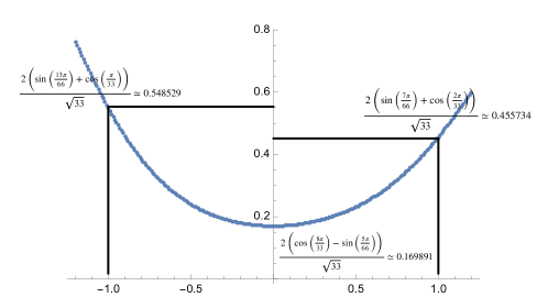
Figure 3: Graph of $|Z_{S^{3}_{b}}(b^{2}=1,M=0,\nu)|$ for $\widetilde{{\cal T}}_{(3,11)}$ theory. The round 3-sphere partition function is minimized at $\nu=0$. The values at $\nu=-1$, $\nu=0$ and $\nu=1$ are identical to the $|S_{(1,1),(1,1)}|$, $|S_{(1,1),(1,3)}|$ and $|S_{(1,1),(1,9)}|$ of $SM(3,11)$ respectively.

For the superconformal index we find that

$$\begin{split}&r=3:\\ &1-q+\left(-\eta-\frac{1}{\eta}\right)q^{3/2}-2q^{2}+\left(\eta^{2}+\frac{1}{\eta^{2}}+1\right)q^{3}+\left(2\eta+\frac{2}{\eta}\right)q^{7/2}+\left(\frac{1}{\eta^{2}}+3\right)q^{4}\\ &+\left(-\eta^{3}+3\eta+\frac{5}{\eta}\right)q^{9/2}+\left(\frac{3}{\eta^{2}}+8\right)q^{5}+\left(-\eta^{3}+3\eta+\frac{7}{\eta}\right)q^{11/2}+\ldots\\ &\textrm{For all $r\geq 3$}:\\ &{\cal I}_{\rm sci}(q;\eta,\nu=0)=1-q-\left(\eta+\frac{1}{\eta}\right)q^{\frac{3}{2}}+\ldots\;,\\ &{\cal I}_{\rm sci}(\eta=1,\nu=\pm 1)=1\;.\end{split}$$ (110)

The index also shows evidences for the SUSY enhancement, ${\cal N}=2\rightarrow{\cal N}=4$, and being of rank 0 SCFT in the IR.

In the twisted partition computation, there are $(3r-4)$ Bethe-vacua, $\{\vec{z}_{\alpha}\}_{\alpha=0}^{3r-5}$, and their handle-gluing/fibering operators in the A-twisting limit, $\vec{M}\rightarrow\vec{0}$ and $\vec{\nu}\rightarrow-2\vec{A}$, are

$$\begin{split}&{\cal H}(\vec{z}_{\alpha};\vec{M}=0,\vec{\nu}=\vec{0})=(S_{(1,1),(1,2\alpha+1)})^{-2}\;,\\ &\left({\cal F}(\vec{z}_{\alpha};\vec{M}=0,\vec{\nu}=\vec{0})\right)^{2}=e^{2\pi i\delta}\exp\left(4\pi ih_{(s=1,t=2\alpha+1)}\right)\;.\end{split}$$ (111)

with a $\delta\in\mathbb{Q}$. Here $S$ and $h_{(s,t)}$ is the S-matrix (6) and conformal dimensions (3) of $SM(3,6r-7)$.

The half-index for the $\widetilde{{\cal T}}_{(3,6r-7)}$ theory is

$$\begin{split}I_{\rm half}(q;\eta,\nu)&=I^{(K,Q)}_{\rm half}(q;\vec{\eta},\vec{\nu}=(\nu-1)\vec{A})\big{|}_{\eta_{a}\rightarrow\eta^{A_{a}}}\\ &=\sum_{\mathbf{m}\in(\mathbb{Z}_{\geq 0})^{r}}\frac{q^{\frac{1}{2}\mathbf{m}\cdot K\cdot\mathbf{m}}(\eta(-q^{1/2})^{(\nu-1)})^{-\vec{A}\cdot\mathbf{m}}}{(q)_{\mathbf{m}_{1}}\ldots(q)_{\mathbf{m}_{r-1}}(q)_{2\mathbf{m}_{r}}}\;.\end{split}$$ (112)

The half-index in the A-twisting limit, $\eta\rightarrow 1$ and $\nu\rightarrow-1$, reproduces the vacuum character the supersymmetric minimal model $SM(3,6r-7)$ up to an decoupled free-fermion character

$$\begin{split}&I_{\rm half}(q;\eta=1,\nu=-1)=\sum_{\mathbf{m}\in(\mathbb{Z}_{\geq 0})^{r}}\frac{q^{\frac{1}{2}\mathbf{m}\cdot K\cdot\mathbf{m}+\vec{A}\cdot\mathbf{m}}}{(q)_{m_{1}}\ldots(q)_{m_{r-1}}(q)_{2m_{r}}}\;\\ &=q^{\frac{c}{24}+\frac{1}{48}}\times\left(\chi_{(1,1)}(q)\textrm{ of }SM(3,6r-7)\textrm{ in \eqref{SM-characters}}\right)\times\left(\chi_{F}(q)\textrm{ in \eqref{free-fermion character}}\right)\;.\end{split}$$ (113)

Here the matrix $K$ and the vector $\vec{A}$ is given in (106) and (107) respectively.

The non-trivial identities in (111) and (113) strongly support the proposal in (105).

3 Summary and Future directions

In this paper, we propose bulk 3D ${\cal N}=4$ rank-0 theories which are related to the ${\cal N}=1$ supersymmetric minimal models $SM(2,\cdot)$ and $SM(3,\cdot)$ via the bulk-boundary correspondence. Like most rank-0 SCFTs, the SCFTs are realized as IR fixed points of UV gauge theories with less supersymmetry (${\cal N}=2$) except for the examples in section 2.2.3 which have manifest ${\cal N}=5$ supersymmetry. We support the proposal by checking the dictionaries in the Table 1 with explicit computations of supersymmetric partition functions.

It would be interesting to generalize our work to other examples of RCFTs and see if there are some non-unitary RCFTs which can not be realized from 3D rank-0 SCFTs. The strongest form of the non-unitary bulk-boundary correspondence can be stated as that every non-unitary chiral RCFTs can be realized as boundary algebras of 3D rank-0 SCFTs. If true, it would be a crucial advantage of 3D non-unitary bulk-boundary correspondence over (4D SCFTs)/(2D VOAs) correspondence in which only a few classes of non-unitary rational algebra can be realized Song:2017oew ; Beem:2017ooy ; Arakawa:2017fdq ; Xie:2019vzr . So far, we could find bulk dual rank-0 SCFTs only for some examples of minimal models, $M(p,q)$ with $p=2$, and supersymmetric minimal models, $SM(p,p^{\prime})$ with $p=2$ and $p=3$. What about other cases? In the upcoming papers Gang:2024tlp ; BGK , bulk field theories for general minimal models and supersymmetric minimal models are proposed using the 3D-3D correspondence Terashima:2011qi ; Dimofte:2011ju ; Gang:2018wek ; Cho:2020ljj ; Choi:2022dju ; Bonetti:2024cvq .

In this paper, the supersymmetric minimal models arise from topological A-twisting of the bulk rank-0 SCFTs. It would be interesting to study the boundary chiral algebras of the topologically B-twisted theories and see how the two chiral algebras from A- and B- twistings are related to each other. For the $M(2,q)$ case, the relation was recently studied in Ferrari:2023fez .

Appendix A Quantum dilogarithm and tetrahedron index

The quantum dilogarithm function $\psi_{\hbar}(Z)$ ($\hbar:=2\pi ib^{2}$) is defined by Faddeev:1993rs

$$\psi_{\hbar}(Z):=\begin{cases}\prod_{r=1}^{\infty}\frac{1-q^{r}e^{-Z}}{1-\widetilde{q}^{-r+1}e^{-\widetilde{Z}}}\;,\quad\textrm{if $|q|<1$}\\ \prod_{r=1}^{\infty}\frac{1-\widetilde{q}^{r}e^{-\widetilde{Z}}}{1-q^{-r+1}e^{-Z}}\;,\quad\textrm{if $|q|>1$}\end{cases}$$ (114)

with

$$q=e^{2\pi ib^{2}},\quad\widetilde{q}:=e^{2\pi ib^{-2}},\quad\widetilde{Z}=Z/b^{2}\;.$$ (115)

The $\psi_{\hbar}(Z)$ computes the squashed 3-sphere partition function of the ${\cal T}_{\Delta}$ theory in (25) with $Z=M+(i\pi+\frac{\hbar}{2}R(\Phi))$, where the $M$ is the rescaled real mass for the $U(1)$ flavor symmetry. In the limit $\hbar\rightarrow 0$, the Q.D.L behaves as follows

$$\begin{split}\log\psi_{\hbar}(Z)\xrightarrow{\;\;\hbar\rightarrow 0\;\;}&\sum_{n=0}^{\infty}\frac{B_{n}\hbar^{n-1}}{n!}{\rm Li}_{2-n}(e^{-Z})=\frac{1}{\hbar}{\rm Li}_{2}(e^{-Z})-\frac{1}{2}\log(1-e^{-Z})+\ldots.\end{split}$$ (116)

Here $B_{n}$ is the $n$-th Bernoulli number with $B_{1}=1$. When $b=1$, on the other hand, the function becomes

$$\psi_{\hbar=2\pi i}(Z)=\exp\left(\frac{-(2\pi+iZ)\log(1-e^{-Z})+i{\rm Li}_{2}(e^{-Z})}{2\pi}\right)\;.$$ (117)

The tetrahedron index ${\cal I}_{\Delta}(m,u)$ is defined as Dimofte:2011py

$$\begin{split}&{\cal I}_{\Delta}(m,u):=\prod_{r=0}^{\infty}\frac{1-q^{r-\frac{1}{2}m+1}u^{-1}}{1-q^{r-\frac{1}{2}m}u}=\sum_{e\in\mathbb{Z}}{\cal I}_{\Delta}^{c}(m,e)u^{e},\;\;\\ &\textrm{where }{\cal I}_{\Delta}^{c}(m,e)=\sum_{n=\lfloor e\rfloor}^{\infty}\frac{(-1)^{n}q^{\frac{1}{2}n(n+1)-(n+\frac{1}{2}e)m}}{(q)_{n}(q)_{n+e}}\;.\end{split}$$ (118)

It computes the generalized superconformal index Kapustin:2011jm of the ${\cal T}_{\Delta}$ theory with the R-charge choice $R(\Phi)=0$ where $(m,u)$ are (background monopole flux, fugacity) for the $U(1)$ flavor symmetry. At general $R$-charge choice, the index becomes ${\cal I}_{\Delta}(m,u(-q^{1/2})^{R(\Phi)})$.

Appendix B Bulk field theories for $M(2,r+2)$ using $K=C(T_{r})^{-1}$ with odd $r$

In section 2.2.2, we propose a UV gauge theory description of ${\cal T}_{(2,2r+4)}$ using mixed CS level $K=C(T_{r})^{-1}$ with even $r$. Here we propose bulk field theories, say $\widetilde{{\cal T}}_{M(2,r+2)}$, for the Virasoro minimal model $M(2,r+2)$ using $K=C(T_{r})^{-1}$ with odd $r$. More precisely, we propose that

$$\begin{split}&\textrm{For $r\in 2\mathbb{Z}_{\geq 1}+1$,}\\ &\widetilde{{\cal T}}_{M(2,r+2)}\xrightarrow{\;\textrm{A-twisting/bulk-boundary}\;}M(2,r+2)\otimes(\textrm{Free fermion}),\end{split}$$ (119)

where

$$\begin{split}&\widetilde{{\cal T}}_{M(2,r+2)}:=\frac{({\cal T}_{\Delta})^{\otimes r}}{[U(1)^{r}_{\mathbf{Q}}]_{K}}\textrm{ with superpotential }{\cal W}={\cal O}_{(\mathbf{m}_{1},\mathbf{n}_{1})}+\ldots+{\cal O}_{(\mathbf{m}_{r-1},\mathbf{n}_{r-1})}\;,\\ &K=C(T_{r})^{-1}:=\begin{pmatrix}1&1&1&\cdots&1&1\\ 1&2&2&\cdots&2&2\\ 1&2&3&\cdots&3&3\\ \vdots&\vdots&\vdots&\ddots&\vdots&\vdots\\ 1&2&3&\cdots&r-1&r-1\\ 1&2&3&\cdots&r-1&r\end{pmatrix},\quad\mathbf{Q}=\mathbb{I}_{r\times r},\\ \hfil\displaystyle\begin{split}&\mathbf{m}_{1}=(1,1,-1,\mathbf{0}_{r-3}),\;\mathbf{m}_{2\leq I\leq r-2}=(\mathbf{0}_{I-2},-1,1,1,-1,\mathbf{0}_{r-I-2}),\;\mathbf{m}_{r-1}=(\mathbf{0}_{r-2},-2,2),\\ &\mathbf{n}_{1\leq I\leq r-1}=(\mathbf{0}_{r})\;.\end{split}\end{split}$$ (120)

The ${\cal N}=2$ gauge theory has a $U(1)$ flavor symmetry, $U(1)_{A}$, whose charge is given as

$$A=\vec{A}\cdot\vec{T}=\sum_{a=1}^{r}\left[\frac{a}{2}\right]T_{a}=T_{2}+T_{3}+2T_{4}+2T_{5}+\ldots+\frac{r-1}{2}T_{r-1}+\frac{r-1}{2}T_{r}\;.$$ (121)

The computation of various BPS partition functions can be done as in the main text. For the superconformal index we find that

$$\begin{split}&{\cal I}_{\rm sci}(q;\eta,\nu=0)=1-q-\left(\eta+\frac{1}{\eta}\right)q^{\frac{3}{2}}+\ldots\;,\\ &{\cal I}_{\rm sci}(\eta=1,\nu=\pm 1)=1\;.\end{split}$$ (122)

The index shows the evidence for the SUSY enhancement, ${\cal N}=2\rightarrow{\cal N}=4$, in the IR. In the twisted partition computation, there are $\frac{r+1}{2}$ Bethe-vacua, $\{\vec{z}_{\alpha}\}_{\alpha=0}^{\frac{r-1}{2}}$. Their handle-gluing/fibering operators in the A-twisting limit, $\vec{M}\rightarrow\vec{0}$ and $\vec{\nu}\rightarrow-2\vec{A}$, are

$$\begin{split}&{\cal H}(\vec{z}_{\alpha};\vec{M}=0,\vec{\nu}=-2\vec{A})=(S_{0,\alpha})^{-2}\;,\\ &\left({\cal F}(\vec{z}_{\alpha};\vec{M}=0,\vec{\nu}=-2\vec{A})\right)^{2}=e^{2\pi i\delta}\exp\left(4\pi ih_{\alpha}\right)\;.\end{split}$$ (123)

with a $\delta\in\mathbb{Q}$. Here $S$ and $h_{\alpha}$ are the S-matrix and conformal dimensions of $M(2,r+2)$:

$$\begin{split}&S_{\alpha,\beta}=\frac{2(-1)^{\frac{r-1}{2}+\alpha+\beta}}{\sqrt{r+2}}\sin\left(\frac{2\pi(\alpha+1)(\beta+1)}{r+2}\right)\;,\\ &h_{\alpha}=\frac{\alpha(\alpha-r)}{2r+4}\;.\end{split}$$ (124)

Let $\{L_{\alpha}\}_{\alpha=0,1,\ldots,\frac{r-1}{2}}$ be supersymmetric Wilson loop operators with gauge charge $\vec{\mathfrak{q}}_{\alpha}$:

$$\vec{\mathfrak{q}}_{\alpha}=(0,1,1,2,2,\ldots,\alpha-1,\alpha-1,\alpha,\alpha,\alpha,\ldots,\alpha)\;.$$ (125)

In the A-twisting limit, $\eta\rightarrow 1$ and $\nu\rightarrow-1$, the half-indices reproduce the characters of 2D RCFT $(M(2,r+2))\otimes(\textrm{free Majonara})$

$$\begin{split}&q^{h_{\alpha}-\frac{c}{24}}I^{L_{\alpha}}_{\rm half}(q;\eta=1,\nu=-1)=q^{h_{\alpha}-\frac{c}{24}}\sum_{\mathbf{m}\in(\mathbb{Z}_{\geq 0})^{r}}\frac{q^{\frac{1}{2}\mathbf{m}\cdot K\cdot\mathbf{m}+\vec{A}\cdot\mathbf{m}-\vec{\mathfrak{q}}_{\alpha}\cdot\mathbf{m}}}{(q)_{m_{1}}\ldots(q)_{m_{r}}}\\ &=\left(\chi_{\alpha}(q)\textrm{ of $M(2,r+2)$}\right)\times\left(\chi_{F}(q)\textrm{ in \eqref{free-fermion character}}\right)\;,\end{split}$$ (126)

up to an overall factor $q^{h_{\alpha}-\frac{c}{24}}$ where conformal dimension $h_{\alpha}$ is given in (124) and the central charge $c$ of the product RCFT is

$$c=\frac{3}{2}-\frac{3r^{2}}{r+2}\;,\quad h_{\alpha}=\frac{\alpha(\alpha-r)}{2r+4}\;.$$ (127)

The character $\chi_{\alpha}(q)$ of $M(2,r+2)$ is feigin1983verma ; felder1989brst

$$\begin{split}&\chi_{\alpha}(q)=\frac{q^{-\Delta^{(2,r+2)}_{1,\alpha+1}}}{(q)_{\infty}}\sum_{k\in\mathbb{Z}}\left(q^{\Delta^{(2,r+2)}_{1+4k,\alpha+1}}-q^{\Delta^{(2,r+2)}_{1+4k,-\alpha-1}}\right)\;,\\ &\Delta^{(p,q)}_{r,s}:=\frac{(rq-sp)^{2}-(q-p)^{2}}{4pq}\;.\end{split}$$ (128)

References

- (1) E. Witten, “Quantum field theory and the Jones polynomial,” Commun. Math. Phys. 121 no. 3, (1989) 351–399.
- (2) G. Moore and N. Seiberg, “Classical and quantum conformal field theory,” Communications in Mathematical Physics 123 (1989) 177–254.
- (3) V. G. Turaev, “Modular categories and 3-manifold invariants,” International Journal of Modern Physics B 6 no. 11n12, (1992) 1807–1824.
- (4) D. Gaiotto, A. Kapustin, N. Seiberg, and B. Willett, “Generalized Global Symmetries,” JHEP 02 (2015) 172, arXiv:1412.5148 [hep-th].
- (5) L. Bhardwaj and Y. Tachikawa, “On finite symmetries and their gauging in two dimensions,” JHEP 03 (2018) 189, arXiv:1704.02330 [hep-th].
- (6) C.-M. Chang, Y.-H. Lin, S.-H. Shao, Y. Wang, and X. Yin, “Topological Defect Lines and Renormalization Group Flows in Two Dimensions,” JHEP 01 (2019) 026, arXiv:1802.04445 [hep-th].
- (7) B. Heidenreich, J. McNamara, M. Montero, M. Reece, T. Rudelius, and I. Valenzuela, “Non-invertible global symmetries and completeness of the spectrum,” JHEP 09 (2021) 203, arXiv:2104.07036 [hep-th].
- (8) M. Koide, Y. Nagoya, and S. Yamaguchi, “Non-invertible topological defects in 4-dimensional pure lattice gauge theory,” PTEP 2022 no. 1, (2022) 013B03, arXiv:2109.05992 [hep-th].
- (9) Y. Choi, C. Cordova, P.-S. Hsin, H. T. Lam, and S.-H. Shao, “Noninvertible duality defects in 3+1 dimensions,” Phys. Rev. D 105 no. 12, (2022) 125016, arXiv:2111.01139 [hep-th].
- (10) J. Kaidi, K. Ohmori, and Y. Zheng, “Kramers-Wannier-like Duality Defects in (3+1)D Gauge Theories,” Phys. Rev. Lett. 128 no. 11, (2022) 111601, arXiv:2111.01141 [hep-th].
- (11) G. Moore and N. Seiberg, “Lectures on rcft (rational conformal field theory),” tech. rep., Institute for Advanced Study, Princeton, NJ (USA); Yale Univ., New Haven, CT …, 1989.
- (12) M. E. Fisher, “Yang-lee edge singularity and 3 field theory,” Physical Review Letters 40 no. 25, (1978) 1610.
- (13) J. L. Cardy, “Conformal invariance and the yang-lee edge singularity in two dimensions,” Physical review letters 54 no. 13, (1985) 1354.
- (14) C. Beem, M. Lemos, P. Liendo, W. Peelaers, L. Rastelli, and B. C. van Rees, “Infinite Chiral Symmetry in Four Dimensions,” Commun. Math. Phys. 336 no. 3, (2015) 1359–1433, arXiv:1312.5344 [hep-th].
- (15) C. Beem, L. Rastelli, and B. C. van Rees, “ symmetry in six dimensions,” JHEP 05 (2015) 017, arXiv:1404.1079 [hep-th].
- (16) B. Feigin and S. Gukov, “VOA[],” J. Math. Phys. 61 no. 1, (2020) 012302, arXiv:1806.02470 [hep-th].
- (17) M. C. N. Cheng, S. Chun, F. Ferrari, S. Gukov, and S. M. Harrison, “3d Modularity,” JHEP 10 (2019) 010, arXiv:1809.10148 [hep-th].
- (18) K. Costello and D. Gaiotto, “Vertex Operator Algebras and 3d = 4 gauge theories,” JHEP 05 (2019) 018, arXiv:1804.06460 [hep-th].
- (19) K. Costello, T. Dimofte, and D. Gaiotto, “Boundary Chiral Algebras and Holomorphic Twists,” Commun. Math. Phys. 399 no. 2, (2023) 1203–1290, arXiv:2005.00083 [hep-th].
- (20) M. C. N. Cheng, S. Chun, B. Feigin, F. Ferrari, S. Gukov, S. M. Harrison, and D. Passaro, “3-Manifolds and VOA Characters,” Commun. Math. Phys. 405 no. 2, (2024) 44, arXiv:2201.04640 [hep-th].
- (21) J. Song, D. Xie, and W. Yan, “Vertex operator algebras of Argyres-Douglas theories from M5-branes,” JHEP 12 (2017) 123, arXiv:1706.01607 [hep-th].
- (22) C. Beem and L. Rastelli, “Vertex operator algebras, Higgs branches, and modular differential equations,” JHEP 08 (2018) 114, arXiv:1707.07679 [hep-th].
- (23) T. Arakawa, “Representation theory of W-algebras and Higgs branch conjecture,” in International Congress of Mathematicians, pp. 1261–1278. 2018. arXiv:1712.07331 [math.RT].
- (24) D. Xie and W. Yan, “4d SCFTs and lisse W-algebras,” JHEP 04 (2021) 271, arXiv:1910.02281 [hep-th].
- (25) S. Gukov, P.-S. Hsin, H. Nakajima, S. Park, D. Pei, and N. Sopenko, “Rozansky-Witten geometry of Coulomb branches and logarithmic knot invariants,” J. Geom. Phys. 168 (2021) 104311, arXiv:2005.05347 [hep-th].
- (26) T. Creutzig, T. Dimofte, N. Garner, and N. Geer, “A QFT for non-semisimple TQFT,” arXiv:2112.01559 [hep-th].
- (27) D. Gang and M. Yamazaki, “Three-dimensional gauge theories with supersymmetry enhancement,” Phys. Rev. D 98 no. 12, (2018) 121701, arXiv:1806.07714 [hep-th].
- (28) D. Gang, S. Kim, K. Lee, M. Shim, and M. Yamazaki, “Non-unitary TQFTs from 3D = 4 rank 0 SCFTs,” JHEP 08 (2021) 158, arXiv:2103.09283 [hep-th].
- (29) K. Costello, T. Creutzig, and D. Gaiotto, “Higgs and Coulomb branches from vertex operator algebras,” JHEP 03 (2019) 066, arXiv:1811.03958 [hep-th].
- (30) C. Beem and A. E. V. Ferrari, “Free field realisation of boundary vertex algebras for Abelian gauge theories in three dimensions,” arXiv:2304.11055 [hep-th].
- (31) A. E. V. Ferrari, N. Garner, and H. Kim, “Boundary vertex algebras for 3d rank-0 SCFTs,” arXiv:2311.05087 [hep-th].
- (32) D. Gang, H. Kim, and S. Stubbs, “Three-Dimensional Topological Field Theories and Nonunitary Minimal Models,” Phys. Rev. Lett. 132 no. 13, (2024) 131601, arXiv:2310.09080 [hep-th].
- (33) D. Gang and D. Kim, “Generalized non-unitary Haagerup-Izumi modular data from 3D S-fold SCFTs,” JHEP 03 (2023) 185, arXiv:2211.13561 [hep-th].
- (34) D. Gang, D. Kim, and S. Lee, “A non-unitary bulk-boundary correspondence: Non-unitary Haagerup RCFTs from S-fold SCFTs,” arXiv:2310.14877 [hep-th].
- (35) M. Dedushenko, S. Gukov, H. Nakajima, D. Pei, and K. Ye, “3d TQFTs from Argyres–Douglas theories,” J. Phys. A 53 no. 43, (2020) 43LT01, arXiv:1809.04638 [hep-th].
- (36) M. Dedushenko, “On the 4d/3d/2d view of the SCFT/VOA correspondence,” arXiv:2312.17747 [hep-th].
- (37) D. L. Jafferis, I. R. Klebanov, S. S. Pufu, and B. R. Safdi, “Towards the F-Theorem: N=2 Field Theories on the Three-Sphere,” JHEP 06 (2011) 102, arXiv:1103.1181 [hep-th].
- (38) H. Casini, M. Huerta, R. C. Myers, and A. Yale, “Mutual information and the F-theorem,” JHEP 10 (2015) 003, arXiv:1506.06195 [hep-th].
- (39) S. Kim, “The Complete superconformal index for N=6 Chern-Simons theory,” Nucl. Phys. B821 (2009) 241–284, arXiv:0903.4172 [hep-th]. [Erratum: Nucl. Phys.B864,884(2012)].
- (40) Y. Imamura and S. Yokoyama, “Index for three dimensional superconformal field theories with general R-charge assignments,” JHEP 04 (2011) 007, arXiv:1101.0557 [hep-th].
- (41) A. Kapustin, B. Willett, and I. Yaakov, “Exact Results for Wilson Loops in Superconformal Chern-Simons Theories with Matter,” JHEP 03 (2010) 089, arXiv:0909.4559 [hep-th].
- (42) D. L. Jafferis, “The Exact Superconformal R-Symmetry Extremizes Z,” JHEP 05 (2012) 159, arXiv:1012.3210 [hep-th].
- (43) N. Hama, K. Hosomichi, and S. Lee, “Notes on SUSY Gauge Theories on Three-Sphere,” JHEP 03 (2011) 127, arXiv:1012.3512 [hep-th].
- (44) N. Hama, K. Hosomichi, and S. Lee, “SUSY Gauge Theories on Squashed Three-Spheres,” JHEP 05 (2011) 014, arXiv:1102.4716 [hep-th].
- (45) F. Benini and A. Zaffaroni, “A topologically twisted index for three-dimensional supersymmetric theories,” JHEP 07 (2015) 127, arXiv:1504.03698 [hep-th].
- (46) F. Benini and A. Zaffaroni, “Supersymmetric partition functions on Riemann surfaces,” Proc. Symp. Pure Math. 96 (2017) 13–46, arXiv:1605.06120 [hep-th].
- (47) C. Closset and H. Kim, “Comments on twisted indices in 3d supersymmetric gauge theories,” JHEP 08 (2016) 059, arXiv:1605.06531 [hep-th].
- (48) C. Closset, H. Kim, and B. Willett, “Supersymmetric partition functions and the three-dimensional A-twist,” JHEP 03 (2017) 074, arXiv:1701.03171 [hep-th].
- (49) C. Closset, H. Kim, and B. Willett, “Seifert fibering operators in 3d theories,” JHEP 11 (2018) 004, arXiv:1807.02328 [hep-th].
- (50) A. Gadde, S. Gukov, and P. Putrov, “Walls, Lines, and Spectral Dualities in 3d Gauge Theories,” JHEP 05 (2014) 047, arXiv:1302.0015 [hep-th].
- (51) A. Gadde, S. Gukov, and P. Putrov, “Fivebranes and 4-manifolds,” Prog. Math. 319 (2016) 155–245, arXiv:1306.4320 [hep-th].
- (52) Y. Yoshida and K. Sugiyama, “Localization of three-dimensional supersymmetric theories on ,” PTEP 2020 no. 11, (2020) 113B02, arXiv:1409.6713 [hep-th].
- (53) T. Dimofte, D. Gaiotto, and N. M. Paquette, “Dual boundary conditions in 3d SCFT’s,” JHEP 05 (2018) 060, arXiv:1712.07654 [hep-th].
- (54) T. Dimofte, D. Gaiotto, and S. Gukov, “Gauge Theories Labelled by Three-Manifolds,” Commun. Math. Phys. 325 (2014) 367–419, arXiv:1108.4389 [hep-th].
- (55) F. Benini, C. Closset, and S. Cremonesi, “Quantum moduli space of Chern-Simons quivers, wrapped D6-branes and AdS4/CFT3,” JHEP 09 (2011) 005, arXiv:1105.2299 [hep-th].
- (56) T. Dimofte, D. Gaiotto, and S. Gukov, “3-Manifolds and 3d Indices,” Adv. Theor. Math. Phys. 17 no. 5, (2013) 975–1076, arXiv:1112.5179 [hep-th].
- (57) A. Kapustin and B. Willett, “Generalized Superconformal Index for Three Dimensional Field Theories,” arXiv:1106.2484 [hep-th].
- (58) C. Cordova, T. T. Dumitrescu, and K. Intriligator, “Multiplets of Superconformal Symmetry in Diverse Dimensions,” JHEP 03 (2019) 163, arXiv:1612.00809 [hep-th].
- (59) M. Evtikhiev, “Studying superconformal symmetry enhancement through indices,” JHEP 04 (2018) 120, arXiv:1708.08307 [hep-th].
- (60) S. S. Razamat and B. Willett, “Down the rabbit hole with theories of class ,” JHEP 10 (2014) 099, arXiv:1403.6107 [hep-th].
- (61) D. Gang and M. Yamazaki, “Expanding 3d = 2 theories around the round sphere,” JHEP 02 (2020) 102, arXiv:1912.09617 [hep-th].
- (62) E. Melzer, “Supersymmetric analogs of the Gordon-Andrews identities, and related TBA systems,” arXiv:hep-th/9412154.
- (63) K. Hosomichi, K.-M. Lee, S. Lee, S. Lee, and J. Park, “N=5,6 Superconformal Chern-Simons Theories and M2-branes on Orbifolds,” JHEP 09 (2008) 002, arXiv:0806.4977 [hep-th].
- (64) D. Gang, H. Kang, and S. Kim, “Non-hyperbolic 3-manifolds and 3D field theories for 2D Virasoro minimal models,” arXiv:2405.16377 [hep-th].
- (65) S. Baek, D. Gang, and H. Kang, “Non-hyperbolic 3-manifolds, 3d rank-0 scfts and supersymmetric minimal models.” work in progress.
- (66) Y. Terashima and M. Yamazaki, “SL(2,R) Chern-Simons, Liouville, and Gauge Theory on Duality Walls,” JHEP 08 (2011) 135, arXiv:1103.5748 [hep-th].
- (67) D. Gang and K. Yonekura, “Symmetry enhancement and closing of knots in 3d/3d correspondence,” arXiv:1803.04009 [hep-th].
- (68) G. Y. Cho, D. Gang, and H.-C. Kim, “M-theoretic Genesis of Topological Phases,” JHEP 11 (2020) 115, arXiv:2007.01532 [hep-th].
- (69) S. Choi, D. Gang, and H.-C. Kim, “Infrared phases of 3D class R theories,” JHEP 11 (2022) 151, arXiv:2206.11982 [hep-th].
- (70) F. Bonetti, S. Schafer-Nameki, and J. Wu, “MTC: 3d Topological Order Labeled by Seifert Manifolds,” arXiv:2403.03973 [hep-th].
- (71) L. D. Faddeev and R. M. Kashaev, “Quantum Dilogarithm,” Mod. Phys. Lett. A 9 (1994) 427–434, arXiv:hep-th/9310070.
- (72) R. Comi, W. Harding, and N. Mekareeya, “Chern-Simons-Trinion theories: One-form symmetries and superconformal indices,” JHEP 09 (2023) 060, arXiv:2305.07055 [hep-th].
- (73) B. L. Feigin and D. Fuks, “Verma modules over the virasoro algebra,” Functional Analysis and its Applications 17 no. 3, (1983) 241–242.
- (74) G. Felder, “Brst approach to minimal models,” Nuclear Physics B 317 no. 1, (1989) 215–236.