SubGDiff: A Subgraph Diffusion Model to Improve Molecular Representation Learning
Abstract
Molecular representation learning has shown great success in advancing AI-based drug discovery. The core of many recent works is based on the fact that the 3D geometric structure of molecules provides essential information about their physical and chemical characteristics. Recently, denoising diffusion probabilistic models have achieved impressive performance in 3D molecular representation learning. However, most existing molecular diffusion models treat each atom as an independent entity, overlooking the dependency among atoms within the molecular substructures. This paper introduces a novel approach that enhances molecular representation learning by incorporating substructural information within the diffusion process. We propose a novel diffusion model termed SubGDiff for involving the molecular subgraph information in diffusion. Specifically, SubGDiff adopts three vital techniques: i) subgraph prediction, ii) expectation state, and iii) -step same subgraph diffusion, to enhance the perception of molecular substructure in the denoising network. Experimentally, extensive downstream tasks demonstrate the superior performance of our approach. The code is available at Github.
.tocmtchapter \etocsettagdepthmtchaptersubsection \etocsettagdepthmtappendixnone
1 Introduction
Molecular representation learning (MRL) has attracted tremendous attention due to its significant role in learning from limited labeled data for applications like AI-based drug discovery (Shen & Nicolaou, 2019; Zhang et al., 2022b, a) and material science (Pollice et al., 2021). From the perspective of physical chemistry, the 3D molecular conformation is crucial to determine the properties of molecules and the activities of drugs (Cruz-Cabeza & Bernstein, 2014). This has spurred the development of numerous geometric neural network architectures and self-supervised learning strategies aimed at leveraging 3D molecular structures to enhance performance on downstream molecular property prediction tasks (Schütt et al., 2017; Zaidi et al., 2023; Liu et al., 2023a).
Diffusion probabilistic models (DPMs) have shown remarkable power to generate realistic samples, especially in synthesizing high-quality images and videos (Sohl-Dickstein et al., 2015; Ho et al., 2020). By modeling the generation as a reverse diffusion process, DPMs transform a random noise into a sample in the target distribution. Recently, diffusion models have been successfully applied to molecular 3D conformation generation (Xu et al., 2022; Jing et al., 2022). The training process in DPMs, which involves reconstructing the original conformation from a noisy version across varying time steps, naturally lends itself to self-supervised representation learning (Pan et al., 2023). Inspired by this, several works have used this technique for molecule pretraining (Liu et al., 2023b; Zaidi et al., 2023). Despite considerable progress, the full potential of DPMs in molecular representation learning remains underexplored. This lead us to investigate the question: Can we effectively enhance MRL with the denoising network (noise predictor) of DPM? If yes, how to achieve it?
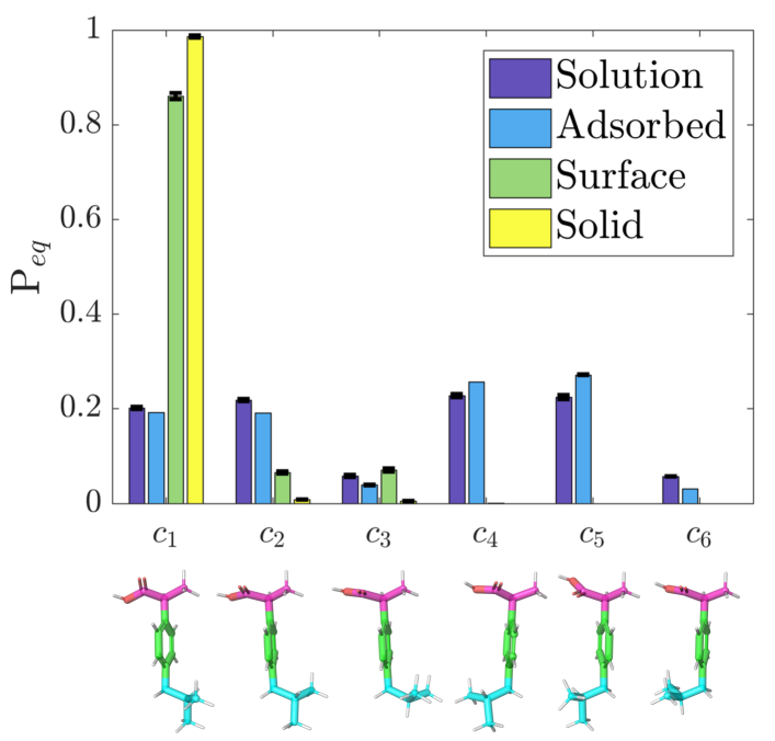
To address this question, we first identify the gap between the current DPMs and the characteristics of molecular structures. Most diffusion models on molecules propose to independently inject continuous Gaussian noise into the every node feature (Hoogeboom et al., 2022) or atomic coordinates of 3D molecular geometry (Xu et al., 2022; Zaidi et al., 2023). However, this approach treats each atom as an individual particle, overlooking the substructure within molecules, which is pivotal in molecular representation learning (Yu & Gao, 2022; Wang et al., 2022a; Miao et al., 2022). As shown in Figure 1, the 3D geometric substructure contains crucial information about the properties, such as the equilibrium distribution, crystallization and solubility (Marinova et al., 2018). As a result, uniformly adding same-scale Gaussian noise to all atoms makes it difficult for the denoising network to capture the properties related to the substructure. So here we try to answer the previous question by designing a DPM involving the knowledge of substructures.
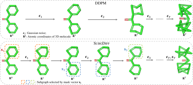
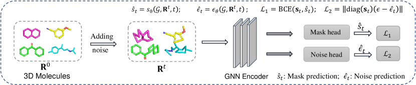
Toward this goal, we propose a novel diffusion model termed SubGDiff, adding distinct Gaussian noise to different substructures of 3D molecular conformation. Specifically, instead of adding the same Gaussian noise to every atomic coordinate, SubGDiff introduces a discrete binary distribution to the diffusion process, where a mask vector sampling from the distribution can be used to select a subset of the atoms (i.e. subgraph) to determine which substructure the noise should be added to at the current time step (Figure 2). More importantly, in the training phase of SubGDiff, a subgraph prediction loss, resembling a node classifier, is integrated. This intentional inclusion explicitly directs the denoising network to capture substructure information from the molecules. Additionally, SubGDiff employs the expectation state diffusion process to bolster its sampling capability and incorporates the k-step same-subgraph diffusion process to optimize the model.
With the ability to capture the substructure information from the noisy 3D molecule, the denoising networks tend to gain more representation power. The experiments on various 2D and 3D molecular property prediction tasks demonstrate the superior performance of our approach. To summarize, our contributions are as follows: (1) we incorporate the substructure information into diffusion models to improve molecular representation learning; (2) we propose a new diffusion model SubGDiff that adopts subgraph prediction, expectation state and -step same-subgraph diffusion to improve its sampling and training; (3) the proposed representation learning method achieves superior performance on various downstream tasks.
2 Related work
Diffusion models on graphs. The diffusion models on graphs can be mainly divided into two categories: continuous diffusion and discrete diffusion. Continuous diffusion applies a Gaussian noise process on each node or edge (Ingraham et al., 2019; Niu et al., 2020), including GeoDiff (Xu et al., 2022), EDM (Hoogeboom et al., 2022), SubDiff (Anonymous, 2024). Meanwhile, discrete diffusion constructs the Markov chain on discrete space, including Digress (Haefeli et al., 2022) and GraphARM (Kong et al., 2023a). However, it remains open to exploring fusing the discrete characteristic into the continuous Gaussian on graph learning, although a closely related work has been proposed for images and cannot be used for generation (Pan et al., 2023). Our work, SubGDiff, is the first diffusion model fusing subgraph, combining discrete characteristics and the continuous Gaussian.
Conformation generation. Various deep generative models have been proposed for conformation generation, including CVGAE (Mansimov et al., 2019), GraphDG (Simm & Hernandez-Lobato, 2020), CGCF (Xu et al., 2021a), ConfVAE (Xu et al., 2021b), ConfGF (Shi et al., 2021) and GeoMol (Ganea et al., 2021). Recently, diffusion-based methods have shown competitive performance. Torsional Diffusion (Jing et al., 2022) raises a diffusion process on the hypertorus defined by torsion angles. However, it is not suitable as a representation learning technique due to the lack of local information (length and angle of bonds). GeoDiff (Xu et al., 2022) generates molecular conformation with a diffusion model on atomic coordinates. However, it views the atoms as separate particles, without considering the dependence between atoms from the substructure.
SSL for molecular property prediction. There exist several works leveraging the 3D molecular conformation to boost the representation learning, including GraphMVP (Liu et al., 2022), GeoSSL (Liu et al., 2023b), the denoising pretraining approach raised by Zaidi et al. (2023) and MoleculeSDE (Liu et al., 2023a), etc. However, those studies have not considered the molecular substructure in the pertaining. In this paper, we concentrate on how to boost the perception of molecular substructure in the denoising networks through the diffusion model.
3 Preliminaries
Notations. We use to denote the identity matrix with dimensionality implied by context, to represent the element product, and to denote the diagonal matrix with diagonal elements of the vector . If not specified, both and represent noise sampled from the standard Gaussian distribution . The topological molecular graph can be denoted as where is the set of nodes, is the set of edges, is the node feature matrix, and its corresponding 3D Conformational Molecular Graph is represented as , where is the set of 3D coordinates of atoms.
DDPM. Denoising diffusion probabilistic models (DDPM) (Ho et al., 2020) is a typical diffusion model (Sohl-Dickstein et al., 2015) which consists of a diffusion (aka forward) and a reverse process. In the setting of molecular conformation generation, the diffusion model adds noise on the 3D molecular coordinates (Xu et al., 2022).
Forward and reverse process. Given the fixed variance schedule , the posterior distribution that is fixed to a Markov chain can be written as
| (1) | |||
| (2) |
To simplify notation, we consider the diffusion on single atom coordinate and omit the subscript to get the general notion throughout the paper. Let , , and then the sampling of at any time step has the closed form: .
The reverse process of DDPM is defined as a Markov chain starting from a Gaussian distribution :
| (3) | |||
| (4) |
where denote time-dependent constant. In DDPM, is parameterized as and , i.e., the denoising network, is parameterized by a neural network where the inputs are and time step .
Training and sampling. The training objective of DDPM is:
| (5) |
After training, samples are generated through the reverse process . Specifically, is first sampled from , and in each step is predicted as follows,
| (6) |
4 SubGDiff
Directly using DDPM on atomic coordinates of 3D molecules means each atom is viewed as an independent single data point. However, the substructures play an important role in molecular generation (Jin et al., 2020) and representation learning (Zang et al., 2023). Ignoring the inherent interactions between atoms may hurt the ability of the denoising network to capture molecular substructure. In this paper, we propose to involve a mask operation in each diffusion step, leading to a new diffusion SubGDiff for molecular representation learning. Each mask corresponds to a subgraph in the molecular graph, aligning with the substructure in the 3D molecule. Furthermore, we incorporate a subgraph predictor and reset the state of the Markov Chain to the expectation of atomic coordinates, thereby enhancing the effectiveness of SubGDiff in sampling. Additionally, we also propose -step same-subgraph diffusion for training to effectively capture the substructure information.
4.1 Involving subgraph into diffusion process
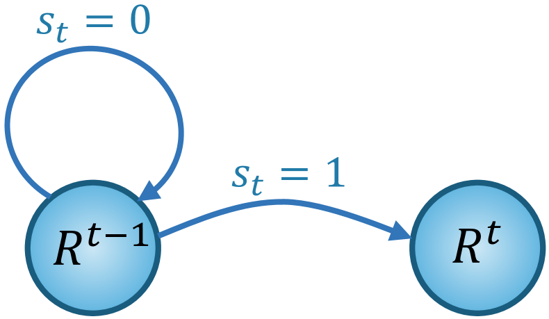
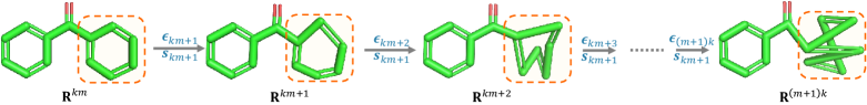
In the forward process of DDPM, we have , in which the Gaussian noise is injected to every atom. Moreover, the training objective in Equation 5 shows that the denoising networks would always predict a Gaussian noise for all atoms. Neither the forward nor reverse process of DDPM takes into account the substructure of the molecule. Instead, in SubGDiff, a mask vector is introduced to determine which atoms will be added noise at step . The mask vector is sampled from a discrete distribution to select a subset of the atoms. In molecular graphs, the discrete mask distribution is equivalent to the subgraph distribution, defined over a predefined sample space , where each sample is a connected subgraph extracted from . Further, the distribution should keep the selected connected subgraph to cohere with the molecular substructures. Here, we adopt a Torsional-based decomposition method (Jing et al., 2022) (Details in Appendix F.1). With the mask vector as latent variables , the state transition of the forward process can be formulated as (Figure 3):
| (7) |
which can be rewritten as . The posterior distribution can be expressed as matrix form:
| (8) | |||
| (9) |
To simplify the notation, we consider the diffusion on a single node and omit the subscript in and to get the notion and . By defining , , the closed form of sampling given is
| (10) |
4.2 Reverse process learning
The reverse process is decomposed as follows:
| (11) |
where and are both learnable models. In the context of molecular learning, the model can be regarded as first predicting which subgraph should be denoised and then using the noise prediction network to denoise the node position in the subgraph.
However, it is tricky to generate a 3D structure by adopting the typical training and sampling method used in Ho et al. (2020). Specifically, following Ho et al. (2020), the reverse process can be optimized by maximizing the variational lower bound (VLB) of as follows,
| (12) | ||||
Details of the derivation are provided in the Appendix C.1. The subgraph predictor in the first term can be parameterized by a node classifier . For the denoising matching term that is closely related to sampling, by Bayes rule, the posterior can be written as:
| (13) | ||||
where is the standard deviation and are contained in . Following DDPM and parameterizing as , the training objective is
|
|
||||
| (14) |
where is the binary cross entropy loss, is the weight used for the trade-off, and is the subgraph predictor implemented as a node classifier with as input and shares a molecule encoder with . The BCE loss employed here uses the subgraph selected at time-step as the target, thereby explicitly compelling the denoising network to capture substructure information from molecules. Eventually, the can be used to infer the mask vector during sampling. Thus, the sampling process is:
| (15) |
However, using Equation 14 and Equation 15 directly for training and sampling faces two issues. First, the inability to access in during the sampling process hinders the step-wise denoising procedure, posing a challenge to the utilization of conventional sampling methods in this context. Inferring solely from using another model is also difficult due to the intricate modulation of noise introduced in through multi-step Gaussian noising. Second, training the subgraph predictor with Equation 14 is challenging. To be specific, the subgraph predictor should be capable of perceiving the sensible noise change between time steps and . However, the noise scale is relatively small when is small, especially if the diffusion step is large (e.g. 1000). As a result, it is difficult to precisely predict the subgraph.
Next, we design two techniques: expectation state diffusion and -step same subgraph diffusion, to effectively tackle the above issues.
4.3 Expectation state diffusion.
To tackle the dilemma above, we first calculate the denoising term in a new way. To eliminate the effect of mask series and improve the training of subgraph prediction loss, we use a new lower bound of the denoising term as follows:
where is defined as
It is an approximated posterior that only relies on the expectation of and . This lower bound defines a new forward process, in which, state to state use the and state remains as Equation 9. Assume each node , (i.i.d. w.r.t. ). Formally, we have
| (16) | |||
| (17) |
where and are general form of and in DDPM (), respectively. Intuitively, this process is equivalent to using mean state to replace during the forward process. This estimation is reasonable since the expectation is like a cluster center of , which can represent properly. Thus, the approximated posterior becomes
| (18) |
where
We parameterize as , and adopt the same training objective as Equation 14. By employing the sampling method , we observe that the proposed expectation state enables a step-by-step execution of the sampling process. Moreover, using expectation is beneficial to reduce the complexity of for predicting the mask during training. This will improve the denoising network to perceive the substructure when we use the diffusion model for self-supervised learning.
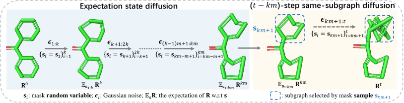
4.4 -step same-subgraph diffusion.
To reduce the complexity of the mask series and accumulate more noise on the same subgraph for facilitating the convergence of the subgraph prediction loss, we generalize the one-step subgraph diffusion to -step same subgraph diffusion (Figure 5 in Appendix), in which the selected subgraph will be continuously diffused steps. After that, the difference between the selected and unselected parts will be distinct enough to help the subgraph predictor perceive it. The forward process of -step same subgraph diffusion can be written as ():
| (19) |
where .
4.5 Training and sampling of SubGDiff
By combining the expectation state and -step same-subgraph diffusion, SubGDiff first divides the entire diffusion step into diffusion intervals. In each interval , the mask vectors are equal to . SubGDiff then adopts the expectation state at the split time step to eliminate the effect of , that is, gets the expectation of at step w.r.t. . Overall, the diffusion process of SubGDiff is a two-phase diffusion process. In the first phase, the state to state use the expectation state diffusion, while in the second phase, state to state use the -step same subgraph diffusion. The state transition refers to Figure 4. With , the two phases can be formulated as follows,
Phase I: Step : where is a general forms of in Equation 17 (in which case ) and . In the rest of the paper, denotes the general version without a special statement. Actually, only calculate the expectation w.r.t. random variables .
Phase II: Step : The phase is a -step same mask diffusion. .
Let , , and . We can drive the single-step state transition: and
| (20) | |||
| (21) |
Then we reuse the training objective in Equation 14 as the objective of SubGDiff:
|
|
||||
| (22) |
where is calculated by Equation 20.
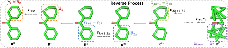
Sampling.
Although the forward process uses the expectation state w.r.t. , we can only update the mask at because sampling only needs to get a subgraph from the distribution in the -step interval. Eventually, adopting the defined in Equation 21, the sampling process is shown below,
|
|
||||
| (23) |
where and . The subgraph selected by will be generated in from the steps to . The mask predictor can be viewed as a discriminator of important subgraphs, indicating the optimal subgraph should be recovered in the next steps. After one subgraph (substructure) is generated properly, the model can gently fine-tune the other parts of the molecule (c.f. the video in supplementary material). This subgraph diffusion would intuitively increase the robustness and generalization of the generation process, which is also verified by the experiments in sec. 5.2. The training and sampling algorithms of SubGDiff are summarized in Alg. 1 and Alg. 2.
Pretraining Aspirin Benzene Ethanol Malonaldehyde Naphthalene Salicylic Toluene Uracil – (random init) 1.203 0.380 0.386 0.794 0.587 0.826 0.568 0.773 Type Prediction 1.383 0.402 0.450 0.879 0.622 1.028 0.662 0.840 Distance Prediction 1.427 0.396 0.434 0.818 0.793 0.952 0.509 1.567 Angle Prediction 1.542 0.447 0.669 1.022 0.680 1.032 0.623 0.768 3D InfoGraph 1.610 0.415 0.560 0.900 0.788 1.278 0.768 1.110 RR 1.215 0.393 0.514 1.092 0.596 0.847 0.570 0.711 InfoNCE 1.132 0.395 0.466 0.888 0.542 0.831 0.554 0.664 EBM-NCE 1.251 0.373 0.457 0.829 0.512 0.990 0.560 0.742 3D InfoMax 1.142 0.388 0.469 0.731 0.785 0.798 0.516 0.640 GraphMVP 1.126 0.377 0.430 0.726 0.498 0.740 0.508 0.620 Denoising 1.364 0.391 0.432 0.830 0.599 0.817 0.628 0.607 GeoSSL 1.107 0.360 0.357 0.737 0.568 0.902 0.484 0.502 MoleculeSDE (VE) 1.112 0.304 0.282 0.520 0.455 0.725 0.515 0.447 MoleculeSDE (VP) 1.244 0.315 0.338 0.488 0.432 0.712 0.478 0.468 Ours 0.880 0.252 0.258 0.459 0.325 0.572 0.362 0.420
5 Experiments
We conduct experiments to address the following two questions: 1) Can substructures improve the representation ability of the denoising network when using diffusion as self-supervised learning? 2) How does the proposed subgraph diffusion affect the generative ability of the diffusion models? For the first question, we employ SubGDiff as a denoising pretraining task and evaluate the performances of the denoising network on various downstream tasks. For the second one, we compare SubGDiff with the vanilla diffusion model GeoDiff (Xu et al., 2022) on the task of molecular conformation generation.
Pre-training BBBP Tox21 ToxCast Sider ClinTox MUV HIV Bace Avg – (random init) 68.10.59 75.30.22 62.10.19 57.01.33 83.72.93 74.62.35 75.20.70 76.72.51 71.60 AttrMask 65.02.36 74.80.25 62.90.11 61.20.12 87.71.19 73.42.02 76.80.53 79.70.33 72.68 ContextPred 65.70.62 74.20.06 62.50.31 62.20.59 77.20.88 75.31.57 77.10.86 76.02.08 71.28 InfoGraph 67.50.11 73.20.43 63.70.50 59.90.30 76.51.07 74.10.74 75.10.99 77.80.88 70.96 MolCLR 66.61.89 73.00.16 62.90.38 57.51.77 86.10.95 72.52.38 76.21.51 71.53.17 70.79 3D InfoMax 68.31.12 76.10.18 64.80.25 60.60.78 79.93.49 74.42.45 75.90.59 79.71.54 72.47 GraphMVP 69.40.21 76.20.38 64.50.20 60.50.25 86.51.70 76.22.28 76.20.81 79.80.74 73.66 MoleculeSDE(VE) 68.30.25 76.90.23 64.70.06 60.20.29 80.82.53 76.81.71 77.01.68 79.91.76 73.15 MoleculeSDE(VP) 70.11.35 77.00.12 64.00.07 60.81.04 82.63.64 76.63.25 77.31.31 81.40.66 73.73 Ours 70.22.23 77.20.39 65.00.48 62.20.97 88.21.57 77.31.17 77.60.51 82.10.96 74.85
5.1 SubGDiff improves molecule representation learning for molecular property prediction
To verify the introduced substructure in the diffusion can enhance the denoising network for representation learning, we pretrain with our SubGDiff objective and finetune on different downstream tasks.
Dataset and settings. For pretraining, we follow (Liu et al., 2023a) and use PCQM4Mv2 dataset (Hu et al., 2020a). It’s a sub-dataset of PubChemQC (Nakata & Shimazaki, 2017) with 3.4 million molecules with 3D geometric conformations. We use various molecular property prediction datasets as downstream tasks. For tasks with 3D conformations, we consider the dataset MD17 and follow the literature (Schütt et al., 2017, 2021; Liu et al., 2023b) of using 1K for training and 1K for validation, while the test set (from 48K to 991K) is much larger.
For downstream tasks with only 2D molecule graphs, we use eight molecular property prediction tasks from MoleculeNet (Wu et al., 2017).
Pretraining framework. To explore the potential of the proposed method for representation learning, we consider MoleculeSDE (Liu et al., 2023a), a SOTA pretraining framework, to be the training backbone, where SubGDiff is used for the model and the mask operation is extended to the node feature and graph adjacency for the model. The details can be found in Appendix F.4.2.
Baselines. For 3D tasks, we incorporate two self-supervised methods [Type Prediction, Angle Prediction], and three contrastive methods [InfoNCE (Oord et al., 2018) and EBM-NCE (Liu et al., 2022) and 3D InfoGraph (Liu et al., 2023b)]. Two denoising baselines are also included [GeoSSL (Liu et al., 2023b), Denoising (Zaidi et al., 2023) and MoleculeSDE]. For 2D tasks, the baselines are AttrMask, ContexPred (Hu et al., 2020b), InfoGraph (Sun et al., 2020), MolCLR (Wang et al., 2022b), 3D InfoMax (Stärk et al., 2022), GraphMVP (Liu et al., 2022) and MoleculeSDE. For details, see Appendix F.4.
Results. As shown in Table 1 and Table 2, SubGDiff outperforms MoleculeSDE in most downstream tasks. The results demonstrate that the introduced mask vector helps the perception of molecular substructure in the denoising network during pretraining. Further, SubGDiff achieves SOTA performance compared to all the baselines. This also reveals that the proposed SubGDiff objective is promising for molecular representation learning due to the involvement of the prior knowledge of substructures during training. More results on the QM9 dataset (Schütt et al., 2017) can be found in Appendix F.4.3.
5.2 SubGDiff benefits conformation generation
We have proposed a new diffusion model to enhance molecular representing learning, where the base diffusion model (GeoDiff) is initially designed for conformation generation. To evaluate the effects of SubGDiff on the generative ability of diffusion models, we evaluate its generation performance and generalization ability.
| COV-R (%) | MAT-R () | COV-P (%) | MAT-P () | |||||||
| Models | Timesteps | Sampling method | Mean | Median | Mean | Median | Mean | Median | Mean | Median |
| GeoDiff | 5000 | DDPM | 80.36 | 83.82 | 0.2820 | 0.2799 | 53.66 | 50.85 | 0.6673 | 0.4214 |
| SubGDiff | 5000 | DDPM (ours) | 90.91 | 95.59 | 0.2460 | 0.2351 | 50.16 | 48.01 | 0.6114 | 0.4791 |
| GeoDiff | 500 | DDPM | 80.20 | 83.59 | 0.3617 | 0.3412 | 45.49 | 45.45 | 1.1518 | 0.5087 |
| SubGDiff | 500 | DDPM (ours) | 89.78 | 94.17 | 0.2417 | 0.2449 | 50.03 | 48.31 | 0.5571 | 0.4921 |
| GeoDiff | 200 | DDPM | 69.90 | 72.04 | 0.4222 | 0.4272 | 36.71 | 33.51 | 0.8532 | 0.5554 |
| SubGDiff | 200 | DDPM (ours) | 85.53 | 88.99 | 0.2994 | 0.3033 | 47.76 | 45.89 | 0.6971 | 0.5118 |
| COV-R (%) | MAT-R () | ||||
| Models | Train data | Mean | Median | Mean | Median |
| CVGAE (Mansimov et al., 2019) | QM9 | 0.09 | 0.00 | 1.6713 | 1.6088 |
| Simm & Hernandez-Lobato (2020) | QM9 | 73.33 | 84.21 | 0.4245 | 0.3973 |
| CGCF (Xu et al., 2021a) | QM9 | 78.05 | 82.48 | 0.4219 | 0.3900 |
| ConfVAE (Xu et al., 2021b) | QM9 | 77.84 | 88.20 | 0.4154 | 0.3739 |
| GeoMol (Ganea et al., 2021) | QM9 | 71.26 | 72.00 | 0.3731 | 0.3731 |
| GeoDiff | Drugs | 74.94 | 79.15 | 0.3492 | 0.3392 |
| SubGDiff | Drugs | 83.50 | 88.70 | 0.3116 | 0.3075 |
Dataset and network. Following prior works (Xu et al., 2022), we utilize the GEOM-QM9 (Ramakrishnan et al., 2014) and GEOM-Drugs (Axelrod & Gomez-Bombarelli, 2022) datasets. The former dataset comprises small molecules of up to 9 heavy atoms, while the latter contains larger drug-like compounds. We reuse the data split provided by Xu et al. (2022). For both datasets, the training dataset comprises molecules, each with conformations, resulting in conformations in total. The test split includes distinctive molecules, with conformations for Drugs and conformations for QM9.
Following (Xu et al., 2022), we use an equivariant network GFN as the denoising network for conformation generation. The detailed description of evaluation metrics and model architecture is in Appendix F.2.
Conformation generation. The comparison with GeoDiff on the GEOM-QM9 dataset is reported in Table 3. From the results, it is easy to see that SubGDiff significantly outperforms the GeoDiff baseline on both metrics (COV-R and MAT-R) across different sampling steps. It indicates that by training with the substructure information, SubGDiff has a positive effect on the conformation generation task. Moreover, SubGDiff with 500 steps achieves much better performance than GeoDiff with 5000 steps on 5 out of 8 metrics, which implies our method can accelerate the sampling efficiency (10x).
Domain generalization. To further illustrate the benefits of SubGDiff, we design two cross-domain tasks: (1) Training on QM9 (small molecular with up to 9 heavy atoms) and testing on Drugs (medium-sized organic compounds); (2) Training on Drugs and testing on QM9. The results (Table 4 and Appendix Table 10) show that SubGDiff consistently outperforms GeoDiff and other models trained on the in-domain dataset, demonstrating the introduced substructure effectively enhances the robustness and generalization of the diffusion model.
6 Conclusion
We present a novel diffusion model SubGDiff, which involves the subgraph constraint in the diffusion model by introducing a mask vector to the forward process. Benefiting from the expectation state and -step same-subgraph diffusion, SubGDiff effectively boosts the perception of molecular substructure in the denoising network, thereby achieving state-of-the-art performance at various downstream property prediction tasks. There are several exciting avenues for future work. The mask distribution can be made flexible such that more chemical prior knowledge may be incorporated into efficient subgraph sampling. Besides, the proposed SubGDiff can be generalized to proteins such that the denoising network can learn meaningful secondary structures.
References
- Alcaraz & Strodthoff (2022) Alcaraz, J. L. and Strodthoff, N. Diffusion-based time series imputation and forecasting with structured state space models. Transactions on Machine Learning Research, 2022.
- Anonymous (2024) Anonymous. Subdiff: Subgraph latent diffusion model, 2024. URL https://openreview.net/forum?id=z2avrOUajn.
- Axelrod & Gomez-Bombarelli (2022) Axelrod, S. and Gomez-Bombarelli, R. GEOM, energy-annotated molecular conformations for property prediction and molecular generation. Scientific Data, 9(1):185, 2022.
- Chmiela et al. (2017) Chmiela, S., Tkatchenko, A., Sauceda, H. E., Poltavsky, I., Schütt, K. T., and Müller, K.-R. Machine learning of accurate energy-conserving molecular force fields. Science advances, 3(5):e1603015, 2017.
- Cruz-Cabeza & Bernstein (2014) Cruz-Cabeza, A. J. and Bernstein, J. Conformational polymorphism. Chemical reviews, 114(4):2170–2191, 2014.
- Ganea et al. (2021) Ganea, O., Pattanaik, L., Coley, C., Barzilay, R., Jensen, K., Green, W., and Jaakkola, T. Geomol: Torsional geometric generation of molecular 3d conformer ensembles. Advances in Neural Information Processing Systems, 34:13757–13769, 2021.
- Haefeli et al. (2022) Haefeli, K. K., Martinkus, K., Perraudin, N., and Wattenhofer, R. Diffusion models for graphs benefit from discrete state spaces. In The First Learning on Graphs Conference, 2022.
- Ho et al. (2020) Ho, J., Jain, A., and Abbeel, P. Denoising diffusion probabilistic models. Advances in neural information processing systems, 33:6840–6851, 2020.
- Hoogeboom et al. (2022) Hoogeboom, E., Satorras, V. G., Vignac, C., and Welling, M. Equivariant diffusion for molecule generation in 3d. In International conference on machine learning, pp. 8867–8887. PMLR, 2022.
- Hu et al. (2020a) Hu, W., Fey, M., Zitnik, M., Dong, Y., Ren, H., Liu, B., Catasta, M., and Leskovec, J. Open graph benchmark: Datasets for machine learning on graphs. arXiv preprint arXiv:2005.00687, 2020a.
- Hu et al. (2020b) Hu, W., Liu, B., Gomes, J., Zitnik, M., Liang, P., Pande, V., and Leskovec, J. Strategies for pre-training graph neural networks. In International Conference on Learning Representations (ICLR), 2020b.
- Ingraham et al. (2019) Ingraham, J., Garg, V., Barzilay, R., and Jaakkola, T. Generative models for graph-based protein design. Advances in neural information processing systems, 32, 2019.
- Jin et al. (2020) Jin, W., Barzilay, R., and Jaakkola, T. Hierarchical generation of molecular graphs using structural motifs. In International conference on machine learning, pp. 4839–4848. PMLR, 2020.
- Jing et al. (2022) Jing, B., Corso, G., Chang, J., Barzilay, R., and Jaakkola, T. S. Torsional diffusion for molecular conformer generation. In Advances in Neural Information Processing Systems, 2022.
- Kabsch (1976) Kabsch, W. A solution for the best rotation to relate two sets of vectors. Acta Crystallographica Section A: Crystal Physics, Diffraction, Theoretical and General Crystallography, 32(5):922–923, 1976.
- Kong et al. (2023a) Kong, L., Cui, J., Sun, H., Zhuang, Y., Prakash, B. A., and Zhang, C. Autoregressive diffusion model for graph generation. In Krause, A., Brunskill, E., Cho, K., Engelhardt, B., Sabato, S., and Scarlett, J. (eds.), Proceedings of the 40th International Conference on Machine Learning, volume 202 of Proceedings of Machine Learning Research, pp. 17391–17408. PMLR, 23–29 Jul 2023a. URL https://proceedings.mlr.press/v202/kong23b.html.
- Kong et al. (2023b) Kong, L., Cui, J., Sun, H., Zhuang, Y., Prakash, B. A., and Zhang, C. Autoregressive diffusion model for graph generation. In Krause, A., Brunskill, E., Cho, K., Engelhardt, B., Sabato, S., and Scarlett, J. (eds.), Proceedings of the 40th International Conference on Machine Learning, volume 202 of Proceedings of Machine Learning Research, pp. 17391–17408. PMLR, 23–29 Jul 2023b. URL https://proceedings.mlr.press/v202/kong23b.html.
- Lei et al. (2023) Lei, J., Cheng, P., Ba, Z., and Ren, K. Masked diffusion models are fast learners. arXiv preprint arXiv:2306.11363, 2023.
- Lin et al. (2023) Lin, H., Huang, Y., Zhang, O., Liu, Y., Wu, L., Li, S., Chen, Z., and Li, S. Z. Functional-group-based diffusion for pocket-specific molecule generation and elaboration. In Thirty-seventh Conference on Neural Information Processing Systems, 2023. URL https://openreview.net/forum?id=lRG11M91dx.
- Liu et al. (2019) Liu, S., Demirel, M. F., and Liang, Y. N-gram graph: Simple unsupervised representation for graphs, with applications to molecules. Advances in neural information processing systems, 32, 2019.
- Liu et al. (2022) Liu, S., Wang, H., Liu, W., Lasenby, J., Guo, H., and Tang, J. Pre-training molecular graph representation with 3D geometry. In International Conference on Learning Representations, 2022.
- Liu et al. (2023a) Liu, S., Du, W., Ma, Z.-M., Guo, H., and Tang, J. A group symmetric stochastic differential equation model for molecule multi-modal pretraining. In International Conference on Machine Learning, pp. 21497–21526. PMLR, 2023a.
- Liu et al. (2023b) Liu, S., Guo, H., and Tang, J. Molecular geometry pretraining with SE(3)-invariant denoising distance matching. In The Eleventh International Conference on Learning Representations, 2023b. URL https://openreview.net/forum?id=CjTHVo1dvR.
- Mansimov et al. (2019) Mansimov, E., Mahmood, O., Kang, S., and Cho, K. Molecular geometry prediction using a deep generative graph neural network. Scientific reports, 9(1):20381, 2019.
- Marinova et al. (2018) Marinova, V., Wood, G. P., Marziano, I., and Salvalaglio, M. Dynamics and thermodynamics of ibuprofen conformational isomerism at the crystal/solution interface. Journal of chemical theory and computation, 14(12):6484–6494, 2018.
- Miao et al. (2022) Miao, S., Liu, M., and Li, P. Interpretable and generalizable graph learning via stochastic attention mechanism. In International Conference on Machine Learning, pp. 15524–15543. PMLR, 2022.
- Nakata & Shimazaki (2017) Nakata, M. and Shimazaki, T. Pubchemqc project: a large-scale first-principles electronic structure database for data-driven chemistry. Journal of chemical information and modeling, 57(6):1300–1308, 2017.
- Niu et al. (2020) Niu, C., Song, Y., Song, J., Zhao, S., Grover, A., and Ermon, S. Permutation invariant graph generation via score-based generative modeling. In International Conference on Artificial Intelligence and Statistics, pp. 4474–4484. PMLR, 2020.
- Oord et al. (2018) Oord, A. v. d., Li, Y., and Vinyals, O. Representation learning with contrastive predictive coding. arXiv preprint arXiv:1807.03748, 2018.
- Pan et al. (2023) Pan, Z., Chen, J., and Shi, Y. Masked diffusion as self-supervised representation learner. arXiv preprint arXiv:2308.05695, 2023.
- Pollice et al. (2021) Pollice, R., dos Passos Gomes, G., Aldeghi, M., Hickman, R. J., Krenn, M., Lavigne, C., Lindner-D’Addario, M., Nigam, A., Ser, C. T., Yao, Z., et al. Data-driven strategies for accelerated materials design. Accounts of Chemical Research, 54(4):849–860, 2021.
- Ramakrishnan et al. (2014) Ramakrishnan, R., Dral, P. O., Rupp, M., and Von Lilienfeld, O. A. Quantum chemistry structures and properties of 134 kilo molecules. Scientific data, 1(1):1–7, 2014.
- Schütt et al. (2017) Schütt, K., Kindermans, P.-J., Sauceda Felix, H. E., Chmiela, S., Tkatchenko, A., and Müller, K.-R. Schnet: A continuous-filter convolutional neural network for modeling quantum interactions. Advances in neural information processing systems, 30, 2017.
- Schütt et al. (2021) Schütt, K., Unke, O., and Gastegger, M. Equivariant message passing for the prediction of tensorial properties and molecular spectra. In International Conference on Machine Learning, pp. 9377–9388. PMLR, 2021.
- Shen & Nicolaou (2019) Shen, J. and Nicolaou, C. A. Molecular property prediction: recent trends in the era of artificial intelligence. Drug Discovery Today: Technologies, 32:29–36, 2019.
- Shi et al. (2021) Shi, C., Luo, S., Xu, M., and Tang, J. Learning gradient fields for molecular conformation generation. In International conference on machine learning, pp. 9558–9568. PMLR, 2021.
- Simm & Hernandez-Lobato (2020) Simm, G. and Hernandez-Lobato, J. M. A generative model for molecular distance geometry. In III, H. D. and Singh, A. (eds.), Proceedings of the 37th International Conference on Machine Learning, volume 119, pp. 8949–8958. PMLR, 2020.
- Sohl-Dickstein et al. (2015) Sohl-Dickstein, J., Weiss, E., Maheswaranathan, N., and Ganguli, S. Deep unsupervised learning using nonequilibrium thermodynamics. In International conference on machine learning, pp. 2256–2265. PMLR, 2015.
- Song & Ermon (2019) Song, Y. and Ermon, S. Generative modeling by estimating gradients of the data distribution. In Advances in Neural Information Processing Systems, pp. 11918–11930, 2019.
- Song et al. (2020) Song, Y., Sohl-Dickstein, J., Kingma, D. P., Kumar, A., Ermon, S., and Poole, B. Score-based generative modeling through stochastic differential equations. In International Conference on Learning Representations, 2020.
- Stärk et al. (2022) Stärk, H., Beaini, D., Corso, G., Tossou, P., Dallago, C., Günnemann, S., and Liò, P. 3D infomax improves GNNs for molecular property prediction. In International Conference on Machine Learning, pp. 20479–20502. PMLR, 2022.
- Sun et al. (2020) Sun, F.-Y., Hoffmann, J., Verma, V., and Tang, J. Infograph: Unsupervised and semi-supervised graph-level representation learning via mutual information maximization. In International Conference on Learning Representations (ICLR), 2020.
- Wang et al. (2022a) Wang, Y., Magar, R., Liang, C., and Barati Farimani, A. Improving molecular contrastive learning via faulty negative mitigation and decomposed fragment contrast. Journal of Chemical Information and Modeling, 62(11):2713–2725, 2022a.
- Wang et al. (2022b) Wang, Y., Wang, J., Cao, Z., and Barati Farimani, A. Molecular contrastive learning of representations via graph neural networks. Nature Machine Intelligence, 4(3):279–287, 2022b.
- Wu et al. (2017) Wu, Z., Ramsundar, B., Feinberg, E. N., Gomes, J., Geniesse, C., Pappu, A. S., Leswing, K., and Pande, V. MoleculeNet: a benchmark for molecular machine learning. Chemical science, 9(2):513–530, 2017.
- Xu et al. (2018) Xu, K., Hu, W., Leskovec, J., and Jegelka, S. How powerful are graph neural networks? In International Conference on Learning Representations, 2018.
- Xu et al. (2021a) Xu, M., Luo, S., Bengio, Y., Peng, J., and Tang, J. Learning neural generative dynamics for molecular conformation generation. In International Conference on Learning Representations, 2021a.
- Xu et al. (2021b) Xu, M., Wang, W., Luo, S., Shi, C., Bengio, Y., Gomez-Bombarelli, R., and Tang, J. An end-to-end framework for molecular conformation generation via bilevel programming. In International Conference on Machine Learning, pp. 11537–11547. PMLR, 2021b.
- Xu et al. (2022) Xu, M., Yu, L., Song, Y., Shi, C., Ermon, S., and Tang, J. GeoDiff: A geometric diffusion model for molecular conformation generation. In International Conference on Learning Representations, 2022. URL https://openreview.net/forum?id=PzcvxEMzvQC.
- Xu et al. (2021c) Xu, Z., Luo, Y., Zhang, X., Xu, X., Xie, Y., Liu, M., Dickerson, K., Deng, C., Nakata, M., and Ji, S. Molecule3d: A benchmark for predicting 3d geometries from molecular graphs. arXiv preprint arXiv:2110.01717, 2021c.
- Yu & Gao (2022) Yu, Z. and Gao, H. Molecular representation learning via heterogeneous motif graph neural networks. In International Conference on Machine Learning, pp. 25581–25594. PMLR, 2022.
- Zaidi et al. (2023) Zaidi, S., Schaarschmidt, M., Martens, J., Kim, H., Teh, Y. W., Sanchez-Gonzalez, A., Battaglia, P., Pascanu, R., and Godwin, J. Pre-training via denoising for molecular property prediction. In The Eleventh International Conference on Learning Representations, 2023.
- Zang et al. (2023) Zang, X., Zhao, X., and Tang, B. Hierarchical molecular graph self-supervised learning for property prediction. Communications Chemistry, 6(1):34, 2023.
- Zhang et al. (2022a) Zhang, J., Li, F., Xiao, X., Xu, T., Rong, Y., Huang, J., and Bian, Y. Hypergraph convolutional networks via equivalency between hypergraphs and undirected graphs. In ICML 2022 Workshop on Topology, Algebra, and Geometry in Machine Learning, 2022a.
- Zhang et al. (2022b) Zhang, J., Xiao, X., Huang, L.-K., Rong, Y., and Bian, Y. Fine-tuning graph neural networks via graph topology induced optimal transport. In Raedt, L. D. (ed.), Proceedings of the Thirty-First International Joint Conference on Artificial Intelligence, IJCAI-22, pp. 3730–3736. International Joint Conferences on Artificial Intelligence Organization, 7 2022b. doi: 10.24963/ijcai.2022/518. URL https://doi.org/10.24963/ijcai.2022/518. Main Track.
- Zhang et al. (2023) Zhang, Y., Zhang, Z., Zhong, B., Misra, S., and Tang, J. DiffPack: A torsional diffusion model for autoregressive protein side-chain packing. In Thirty-seventh Conference on Neural Information Processing Systems, 2023. URL https://openreview.net/forum?id=sXMQPKbLXf.
Appendix
.tocmtappendix \etocsettagdepthmtchapternone \etocsettagdepthmtappendixsubsection
Appendix A More Related Works
Masks on diffusion models.
Previous works also share a similar idea of subgraph (mask) diffusion, such as MDM (Pan et al., 2023), MDSM (Lei et al., 2023) and SSSD (Alcaraz & Strodthoff, 2022). However, the difference between our SubGDiff and theirs mainly lies in the following two aspects: i) Usage: the mask matrix/vector in SSSD and MDSM is fixed in all training steps, which means some segments of the data (time series or images) will never be diffused. But our method samples the at each time step, hence a suitable discrete distribution can ensure that almost all nodes can be added noise. ii) Purpose: MDSM and MDM concentrate on self-supervised pre-training, while SubGDiff serves as a potent generative model and self-supervised pre-training algorithm. Notably, when , SubGDiff can recover to MDSM.
Graph generation models.
D3FG (Lin et al., 2023): D3FG adopts three different diffusion models (D3PM, DDPM, and SO(3) Diffusion) to generate three different parts of molecules(linkerr types, center atom position, and functional group orientations), respectively. In general, these three parts can also be viewed as three subgraphs(subset). DiffPACK(Zhang et al., 2023) is an Autoregressive generative method that predicts the torsional angle of protein side-chains with the condition , where is a predefined subset of atoms. It uses a torsional-based diffusion model to approximate the distribution , in which every subset needs a separate score network to estimate. Essentially, both D3FG and DiffPACK can be viewed as selecting a subset first and then only adding noise on the fixed subset during the entire diffusion process. In contrast, our method proposes to randomly sample a subset from mask distribution in each time-step during the forward process. (Kong et al., 2023b) proposes an autoregressive diffusion model named GraphARM, which absorbs one node in each time step by masking it along with its connecting edges during the forward process. Differently from GraphARM, our SubGDiff selects a subgraph in each time step to inject the Gaussian noise, which is equivalent to masking several nodes during the forward process. In addition, the number of steps in GraphARM must be the same as the number of nodes due to the usage of the absorbing state, while our method can set any time-step during diffusion theoretically since we use the real-value Gaussian noise. Concurrently, SubDiff (Anonymous, 2024) is proposed to use subgraphs as minimum units to train a latent diffusion model, while our method directly involves the subgraph during the forward process, which is a new type of diffusion model.
Appendix B An important lemma for diffusion model
According to (Sohl-Dickstein et al., 2015; Ho et al., 2020), the diffusion model is trained by optimizing the variational bound on the negative log-likelihood , in which the tricky terms are , . Here we provide a lemma that tells us the posterior distribution used in the training and sampling algorithms of the diffusion model can be determined by , . Formally, we have
Lemma B.1.
Assume the forward and reverse processes of the diffusion model are both Markov chains. Given the forward Gaussian distribution , and , the distribution is
Parameterizing in the reverse process as , the training objective of the DPM can be written as
and the sampling (reverse) process is
| (24) |
where .
Once we get the variables , we can directly obtain the training objective and sampling process via lemma B.1, which will help the design of new diffusion models.
Proof:
Given the forward Gaussian distribution and , we have
| (25) |
From the DDPM, we know training a diffusion model should optimize the ELBO of the data
|
|
(26) | |||
| (27) |
To compute the KL divergence , we first rewrite by Bayes rule
| (28) | ||||
| (29) | ||||
| (30) | ||||
| (31) | ||||
| (32) | ||||
| (33) | ||||
| (34) | ||||
| (35) | ||||
| (36) | ||||
| (37) | ||||
| (38) | ||||
| (39) |
We can rewrite our variance equation as , where:
| (40) |
From (25), we have the relationship between and :
| (41) |
Substituting this into , we can get
| (42) | ||||
| (43) | ||||
| (44) | ||||
| (45) |
Thus,
| (46) |
Parameterizing in the reverse process as , and the corresponding optimization problem becomes:
| (47) | |||
| (48) | |||
| (49) | |||
| (50) | |||
| (51) |
Therefore, the training objective of the DPM can be written as
| (52) |
During the reverse process, we sample . Formally, the sampling (reverse) process is
| (53) |
Appendix C Derivations of Training Objectives
C.1 SubGDiff (1-same step and without expectation state)
Here, we utilize the binary characteristic of the mask vector to derive the ELBO for SubGDiff, and we also provide a general proof in sec. C.2:
|
|
(54) | |||
| (55) | ||||
| (56) | ||||
| (57) | ||||
| (58) |
The first term is mask prediction while the second term is similar to the ELBO of the classical diffusion model. The only difference is the in . According to Bayes rule, we can rewrite each transition as:
| (60) |
where is Dirac delta function, that is, if and . Without loss of generality, assume that and both equal . Armed with this new equation, we drive the second term:
| (61) | |||
| (62) | |||
| (63) | |||
| (64) | |||
| (65) | |||
| (66) | |||
| (67) | |||
| (68) | |||
| (69) | |||
| (70) | |||
| (71) | |||
| (72) | |||
| (73) | |||
| (74) |
Here, the decay term represents the terms with , which are unnecessary to minimize when we set . Eventually, the ELOB can be rewritten as follows:
|
|
||||
| (75) | ||||
The mask prediction term can be implemented by a node classifier and the denoising matching term can be calculated via Lemma B.1. In detail,
| (76) | ||||
| (77) |
Thus, the training objective of SubGDiff is:
| (78) |
To recover the existing work, we omit the mask prediction term (i.e. Let ) of SubGDiff in the main text.
C.2 ELBO of SubGDiff
Here, we can derive the ELBO for SubGDiff:
|
|
(79) | |||
| (80) | ||||
| (81) | ||||
| (82) | ||||
| (83) | ||||
| (84) | ||||
| (85) | ||||
| (86) | ||||
| (87) |
According to Bayes rule, we can rewrite each transition as:
| (89) |
Armed with this new equation, we drive the second term:
| (90) | |||
| (91) | |||
| (92) | |||
| (93) | |||
| (94) | |||
| (95) | |||
| (96) | |||
| (97) | |||
| (98) | |||
| (99) | |||
| (100) | |||
| (101) | |||
| (102) | |||
| (103) |
Eventually, the ELOB can be rewritten as follows:
|
|
(104) | |||
| (105) | ||||
The mask prediction term can be implemented by a node classifier . For the denoising matching term, by Bayes rule, the can be written as:
| (106) |
For the naive SubGDiff, we have
| (107) | ||||
| (108) |
Then the denoising matching term can also be calculated via Lemma B.1 (let , and ). Thus, the training objective of SubGDiff is:
| (109) |
C.2.1 Expectation of
The denoising matching term in (105) can be calculated by only sampling instead of . Specifically, we substitute (106) into the denoising matching term:
| (110) | |||
| (111) | |||
| (112) | |||
| (113) | |||
| (114) | |||
| (115) | |||
| (116) | |||
| (117) | |||
| (118) | |||
| (119) |
Thus, we should focus on calculating the distribution
| (120) |
By lemma B.1, if we can gain the expression of and , we can get the training objective and sampling process.
C.3 Single-step subgraph diffusion
C.3.1 Training
I: Step to Step ():
The state space of the mask diffusion should be the mean of the random state.
| (121) |
| (122) |
Form (122), we have:
| (123) | ||||
| (124) | ||||
| (125) | ||||
| (126) | ||||
| (127) | ||||
| (128) | ||||
| (129) | ||||
| (130) | ||||
| (131) | ||||
| (132) |
where and .
| (134) |
II: Step to Step ():
We build the step is a discrete transition from , with
| (135) | ||||
| (136) |
| (137) | ||||
| (138) | ||||
| (139) | ||||
| (140) |
Step to Step ():
| (141) | ||||
| (142) |
Thus, from subsection C.2.1, the training objective of 1-step SubGDiff is:
| (143) |
where is Binary Cross Entropy loss. However, training the SubGDiff is not trivial. The challenges come from two aspects: 1) the mask predictor should be capable of perceiving the sensible noise change between -th and -th step. However, the noise scale is relatively small when is small, especially if the diffusion step is larger than a thousand, thereby mask predictor cannot precisely predict. 2) The accumulated noise for each node at -th step would be mainly affected by the mask sampling from to step, which heavily increases the difficulty of predicting the noise added between -step to -step.
C.3.2 Sampling
Finally, the sampling can be written as:
| (144) | ||||
| (145) | ||||
| (146) |
where and
| (148) |
Appendix D Expectation state distribution
The state space of the mask diffusion should be the mean of the random state.
| (149) |
Form Equation 122, we have:
| (150) | ||||
| (151) | ||||
| (152) | ||||
| (153) | ||||
| (154) | ||||
| (155) | ||||
| (156) | ||||
| (157) | ||||
| (158) | ||||
| (159) | ||||
| (160) | ||||
| (161) | ||||
| (162) |
where and .
Finally, the Expectation state distribution is:
| (164) |
Appendix E The derivation of SubGDiff
When is an integer multiple of ,
| (165) | ||||
| (166) | ||||
| (167) | ||||
| (168) |
where .
When , we have
| (169) | ||||
| (170) | ||||
| (171) | ||||
| (172) | ||||
| (173) |
where .
| (174) | ||||
| (175) |
Let , , and
| (176) |
E.0.1 Sampling
The schematic can see Figure 6.
Appendix F Experiment details and more results
The source code would be available at github. All models are trained with SGD using the ADAM optimizer.
| Task | scheduler | k (k-same mask) | Batch Size | Train Iter. | ||||
| QM9 | 1e-7 | 2e-3 | 5000 | 250 | 10Å | 64 | 2M | |
| Drugs | 1e-7 | 2e-3 | 5000 | 250 | 10Å | 32 | 6M |
| Task | scheduler | k (k-same mask) | Batch Size | Train Iter. | ||||
| 500-step QM9 | 1e-7 | 2e-2 | 500 | 25 | 10Å | 64 | 2M | |
| 200-step QM9 | 1e-7 | 5e-2 | 200 | 10 | 10Å | 64 | 2M | |
| 500-step Drugs | 1e-7 | 2e-2 | 500 | 25 | 10Å | 32 | 4M | |
| 1000-step Drugs | 1e-7 | 9e-3 | 500 | 50 | 10Å | 32 | 4M |
| COV-R (%) | MAT-R () | |||||
| Models | Timesteps | Sampling method | Mean | Median | Mean | Median |
| GeoDiff | 500 | DDPM | 50.25 | 48.18 | 1.3101 | 1.2967 |
| SubGDiff | 500 | DDPM (ours) | 76.16 | 86.43 | 1.0463 | 1.0264 |
| GeoDiff | 500 | LD | 64.12 | 75.56 | 1.1444 | 1.1246 |
| SubGDiff | 500 | LD (ours) | 74.30 | 77.87 | 1.0003 | 0.9905 |
F.1 Mask distribution
In this paper, we pre-define the mask distribution to be a discrete distribution, with sample space , and , where is the subgraph split by the Torsional-based decomposition methods (Jing et al., 2022). The decomposition approach will cut off one torsional edge in a 3D molecule to make the molecule into two components, each of which contains at least two atoms. The two components are represented as two complementary mask vectors (i.e. ). Thus torsional edges in will generate subgraphs. Finally, for each atom , the , i.e. in SubGDiff.
F.2 Conformation Generation
| COV-R (%) | MAT-R () | COV-P (%) | MAT-P () | |||||||
| Steps | Sampling method | Models | Mean | Median | Mean | Median | Mean | Median | Mean | Median |
| 500 | Langevin dynamics | GeoDiff | 87.80 | 93.66 | 0.3179 | 0.3216 | 46.25 | 45.02 | 0.6173 | 0.5112 |
| 500 | Langevin dynamics | SubGDiff | 91.40 | 95.39 | 0.2543 | 0.2601 | 51.71 | 48.50 | 0.5035 | 0.4734 |
| 200 | Langevin dynamics | GeoDiff | 86.60 | 93.09 | 0.3532 | 0.3574 | 42.98 | 42.60 | 0.5563 | 0.5367 |
| 200 | Langevin dynamics | SubGDiff | 90.36 | 95.93 | 0.3064 | 0.3098 | 48.56 | 46.46 | 0.5540 | 0.5082 |
.
Evaluation metrics for conformation generation. To compare the generated and ground truth conformer ensembles, we employ the same evaluation metrics as in a prior study (Ganea et al., 2021): Average Minimum RMSD (AMR) and Coverage. These metrics enable us to assess the quality of the generated conformers from two perspectives: Recall (R) and Precision (P). Recall measures the extent to which the generated ensemble covers the ground-truth ensemble, while Precision evaluates the accuracy of the generated conformers.
The four metrics built upon root-mean-square deviation (RMSD), which is defined as the normalized Frobenius norm of two atomic coordinates matrices, after alignment by Kabsch algorithm (Kabsch, 1976). Formally, let and denote the sets of generated and reference conformers respectively, then the Coverage and Matching metrics (Xu et al., 2021a) can be defined as:
| (185) | ||||
| (186) |
where is a threshold. The other two metrics COV-P and MAT-P can be defined similarly but with the generated sets and reference sets exchanged. In practice, is set as twice of the size of for each molecule.
Settings. For GeoDiff (Xu et al., 2022) with 5000 steps, we use the checkpoints released in public GitHub to reproduce the results. For 200 and 500 steps, we retrain it and do the DDPM sampling.
Comparison with GeoDiff using Langevin Dynamics sampling method.
In order to verify that our proposed diffusion process can bring benefits to other sampling methods, we conduct the experiments to compare our proposed diffusion model with GeoDiff by adopting a typical sampling method Langevin dynamics (LD sampling)(Song & Ermon, 2019) :
| (187) |
where and . is the hyper-parameter referring to step size and is the noise schedule in the forward process. We use various time-step to evaluate the generalization and robustness of the proposed method, and the results shown in Table 8 indicate that our method significantly outperforms GeoDiff, especially when the time-step is relatively small (200,500), which implies that our training method can effectively improve the efficiency of denoising.
| COV-R (%) | MAT-R () | COV-P (%) | MAT-P () | |||||
| Models | Mean | Median | Mean | Median | Mean | Median | Mean | Median |
| CVGAE | 0.09 | 0.00 | 1.6713 | 1.6088 | - | - | - | - |
| GraphDG | 73.33 | 84.21 | 0.4245 | 0.3973 | 43.90 | 35.33 | 0.5809 | 0.5823 |
| CGCF | 78.05 | 82.48 | 0.4219 | 0.3900 | 36.49 | 33.57 | 0.6615 | 0.6427 |
| ConfVAE | 77.84 | 88.20 | 0.4154 | 0.3739 | 38.02 | 34.67 | 0.6215 | 0.6091 |
| GeoMol | 71.26 | 72.00 | 0.3731 | 0.3731 | - | - | - | - |
| ConfGF | 88.49 | 94.31 | 0.2673 | 0.2685 | 46.43 | 43.41 | 0.5224 | 0.5124 |
| GeoDiff | 80.36 | 83.82 | 0.2820 | 0.2799 | 53.66 | 50.85 | 0.6673 | 0.4214 |
| SubGDiff | 90.91 | 95.59 | 0.2460 | 0.2351 | 50.16 | 48.01 | 0.6114 | 0.4791 |
.
Comparison with SOTAs.
i) Baselines: We compare SubGDiff with state-of-the-art baselines: CVGAE (Mansimov et al., 2019), GraphDG (Simm & Hernandez-Lobato, 2020), CGCF (Xu et al., 2021a), ConfVAE (Xu et al., 2021b), ConfGF (Shi et al., 2021) and GeoDiff (Xu et al., 2022). For the above baselines, we reuse the experimental results reported by (Xu et al., 2022). For GeoDiff (Xu et al., 2022), we use the checkpoints released in public GitHub to reproduce the results. ii)Results: The results on the GEOM-QM9 dataset are reported in Table 9. From the results, we get the following observation: SubGDiff significantly outperforms the baselines on COV-R, indicating the SubGDiff tends to explore more possible conformations. This implicitly demonstrates the subgraph will help fine-tune the generated conformation to be a potential conformation.
Model Architecture.
We adopt the graph field network (GFN) from (Xu et al., 2022) as the GNN encoder for extracting the 3D molecular information. In the -th layer, the GFN receives node embeddings (where represents the feature dimension) and corresponding coordinate embeddings as input. It then produces the output and according to the following process:
| (188) | |||
| (189) | |||
| (190) |
where are implemented as feed-forward networks and denotes interatomic distances. The initial embedding is composed of atom embedding and time step embedding while represents atomic coordinates. is the neighborhood of node, consisting of connected atoms and other ones within a radius threshold , helping the model capture long-range interactions explicitly and support disconnected molecular graphs.
Eventually, the Gaussian noise and mask can be predicted as follows (C.f. Figure 7):
| (191) | |||
| (192) |
where is equivalent and is invariant.
F.3 Domain generelizaion
The results of Training on QM9 (small molecular with up to 9 heavy atoms) and testing on Drugs (medium-sized organic compounds) can be found in table 10.
| Train | COV-R (%) | MAT-R () | |||
| Models | data | Mean | Median | Mean | Median |
| CVGAE | Drugs | 0.00 | 0.00 | 3.0702 | 2.9937 |
| GraphDG | Drugs | 8.27 | 0.00 | 1.9722 | 1.9845 |
| GeoDiff | QM9 | 7.99 | 0.00 | 2.7704 | 2.3297 |
| SubGDiff | QM9 | 24.01 | 9.93 | 1.6128 | 1.5819 |
F.4 Self-supervised learning
F.4.1 Model architecture
We use the pretraining framework MoleculeSDE proposed by (Liu et al., 2023a) and extend our SubGDiff to multi-modality pertaining. The two key components of MoleculeSDE are two SDEs(stochastic differential equations Song et al. (2020)): an SDE from 2D topology to 3D conformation () and an SDE from 3D conformation to 2D topology (). In practice, these two SDEs can be replaced by discrete diffusion models. In this paper, we use the proposed SubGDiff to replace the SDEs.
2D topological molecular graph. A topological molecular graph is denoted as , where is the atom attribute matrix and is the bond attribute matrix. The 2D graph representation with graph neural network (GNN) is:
| (193) |
where GIN is the a powerful 2D graph neural network (Xu et al., 2018) and , where is the -th node representation.
3D conformational molecular graph. The molecular conformation is denoted as . The conformational representations are obtained by a 3D GNN SchNet (Schütt et al., 2017):
| (194) |
where , and is the -th node representation.
An SE(3)-Equivariant Conformation Generation
The first objective is the conditional generation from topology to conformation, , implemented as SubGDiff. The denoising network we adopt is the SE(3)-equivariance network () used in MoleculeSDE. The details of the network architecture refer to (Liu et al., 2023a).
Therefore, the training objective from 2D topology graph to 3D confirmation is:
| (195) | ||||
where gets the invariant feature from and introduces a mask head (MLP) to read out the mask prediction.
An SE(3)-Invariant Topology Generation. The second objective is to reconstruct the 2D topology from 3D conformation, i.e., . We also use the SE(3)-invariant score network proposed by MoleculeSDE. The details of the network architecture refer to (Liu et al., 2023a). For modeling , it needs to satisfy the SE(3)-invariance symmetry property. The inputs are 3D conformational representation , the noised 2D information at time , and time . The output of is the Gaussian noise, as . The diffused 2D information contains two parts: . For node feature , the training objective is
|
|
(196) | |||
| (197) |
For edge feature , we define a mask matrix from mask vector : if or , otherwise, . Eventually, the ojective can be written as:
|
|
(198) | |||
| (199) |
Then the score network is also decomposed into two parts for the atoms and bonds: and . Similarly, the mask predictor is also decomposed into two parts for the atoms and bonds: and .
Similar to the topology to conformation generation procedure, the gets the invariant feature from and introduces a mask head (MLP) to read out the mask prediction.
Learning. Following MoleculeSDE, we incorporate a contrastive loss called EBM-NCE (Liu et al., 2022). EBM-NCE provides an alternative approach to estimate the mutual information and is anticipated to complement the generative self-supervised learning (SSL) method. As a result, the ultimate objective is:
| (200) |
where are three coefficient hyperparameters.
F.4.2 Dataset and settings
Dataset. For pretraining, following MoleculeSDE, we use PCQM4Mv2 (Hu et al., 2020a). It’s a sub-dataset of PubChemQC (Nakata & Shimazaki, 2017) with 3.4 million molecules with both the topological graph and geometric conformations.
For finetuning, in addition to QM9 (Ramakrishnan et al., 2014), we also include MD17. To be specific, MD17 comprises eight molecular dynamics simulations focused on small organic molecules. These datasets were initially presented by Chmiela et al. (2017) for the development of energy-conserving force fields using GDML. Each dataset features the trajectory of an individual molecule, encompassing a broad spectrum of conformations. The objective is to predict energies and forces for each trajectory by employing a single model.
Baselines for 3D property prediction
We begin by incorporating three coordinate-MI-unaware SSL methods: (1) Type Prediction, which aims to predict the atom type of masked atoms; (2) Angle Prediction, which focuses on predicting the angle among triplet atoms, specifically the bond angle prediction; (3) 3D InfoGraph, which adopts the contrastive learning paradigm by considering the node-graph pair from the same molecule geometry as positive and negative otherwise. Next, in accordance with the work of (Liu et al., 2023b), we include two contrastive baselines: (4) GeoSSL-InfoNCE (Oord et al., 2018) and (5) GeoSSL-EBM-NCE (Liu et al., 2022). We also incorporate a generative SSL baseline named (6) GeoSSL-RR (RR for Representation Reconstruction). The above baselines are pre-trained on a subset of 1M molecules with 3D geometries from Molecule3D (Xu et al., 2021c) and we reuse the results reported by (Liu et al., 2023b) with SchNet as backbone.
Compared with GeoDiff.
We directly reuse the pre-trained model of the molecular conformation generation in sec. 5.2 for fine-tuning, to compare our method with GeoDiff from naive denoising pretraining perspective (Zaidi et al., 2023). The results are shown in Table 11.
Pretraining Alpha Gap HOMO LUMO Mu Cv G298 H298 R2 U298 U0 Zpve GeoDiff 0.078 51.84 30.88 28.29 0.028 0.035 15.35 11.37 0.132 15.76 15.24 1.869 SubGDiff (ours) 0.076 50.80 31.15 26.62 0.025 0.032 14.92 12.86 0.129 14.74 14.53 1.710
F.4.3 3D molecular property prediction Results on QM9.
By adopting the pertaining setting in Appendix F.4.2, we also take the QM9 dataset for finetuning and follow the literature (Schütt et al., 2017, 2021; Liu et al., 2023a), using 110K for training, 10K for validation and 11k for testing. In addition, the QM9 dataset encompasses 12 tasks that pertain to quantum properties, which are commonly used for evaluating representation learning tasks (Schütt et al., 2017; Liu et al., 2023b). The experimental results can be seen in Table 12. The results also suggest the superior performance of our method.
Pretraining Alpha Gap HOMO LUMO Mu Cv G298 H298 R2 U298 U0 Zpve Random init 0.070 50.59 32.53 26.33 0.029 0.032 14.68 14.85 0.122 14.70 14.44 1.698 Supervised 0.070 51.34 32.62 27.61 0.030 0.032 14.08 14.09 0.141 14.13 13.25 1.727 Type Prediction 0.084 56.07 34.55 30.65 0.040 0.034 18.79 19.39 0.201 19.29 18.86 2.001 Distance Prediction 0.068 49.34 31.18 25.52 0.029 0.032 13.93 13.59 0.122 13.64 13.18 1.676 Angle Prediction 0.084 57.01 37.51 30.92 0.037 0.034 15.81 15.89 0.149 16.41 15.76 1.850 3D InfoGraph 0.076 53.33 33.92 28.55 0.030 0.032 15.97 16.28 0.117 16.17 15.96 1.666 GeossL-RR 0.073 52.57 34.44 28.41 0.033 0.038 15.74 16.11 0.194 15.58 14.76 1.804 GeossL-InfoNCE 0.075 53.00 34.29 27.03 0.029 0.033 15.67 15.53 0.125 15.79 14.94 1.675 GeossL-EBM-NCE 0.073 52.86 33.74 28.07 0.031 0.032 14.02 13.65 0.121 13.70 13.45 1.677 GeossL 0.066 48.59 30.83 25.27 0.028 0.031 13.06 12.33 0.117 12.48 12.06 1.631 MoleculeSDE 0.062 47.74 28.02 24.60 0.028 0.029 13.25 12.70 0.120 12.68 12.93 1.643 Ours 0.054 44.88 25.45 23.75 0.027 0.028 12.03 11.46 0.110 11.32 11.25 1.568
F.5 Visualization
We conduct an alignment analysis to validate that our method can capture chemically informative subgraphs during pretraining. Specifically, we employ t-distributed stochastic neighbor embedding (t-SNE) to represent molecules with various scaffolds visually. The purpose is to investigate whether molecules sharing the same scaffold exhibit similar representations, extracted by the pretrained molecular encoder. A scaffold is usually represented by a substructure of a molecule and can be regarded as the subgraph in our SubGDiff.
In our analysis, we select the nine most prevalent scaffolds from each dataset (BBBP, Sider, ClinTox, and Bace) and assign each molecule to a cluster according to its scaffold. To quantify the molecule embedding, we compute the Silhouette index of the embeddings for each dataset.
As shown in Table 13, SubGDiff enables the generation of more distinctive representations of molecules with different scaffolds. This implies that SubGDiff enables the denoising network (molecular encoder) to better capture the subgraph (scaffold) information. We also provide the t-SNE visualizations in Figure 8.
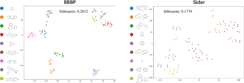
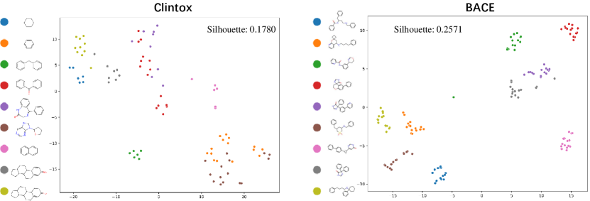
BBBP ToxCast Sider ClinTox Bace MoleculeSDE 0.2344 0.0611 0.1664 0.1394 0.1860 SubGDiff (ours) 0.2632 0.0650 0.1739 0.1780 0.2571