Minimal Perspective Autocalibration

Abstract

We introduce a new family of minimal problems for reconstruction from multiple views. Our primary focus is a novel approach to autocalibration, a long-standing problem in computer vision. Traditional approaches to this problem, such as those based on Kruppa’s equations or the modulus constraint, rely explicitly on the knowledge of multiple fundamental matrices or a projective reconstruction. In contrast, we consider a novel formulation involving constraints on image points, the unknown depths of 3D points, and a partially specified calibration matrix $K$. For $2$ and $3$ views, we present a comprehensive taxonomy of minimal autocalibration problems obtained by relaxing some of these constraints. These problems are organized into classes according to the number of views and any assumed prior knowledge of $K$. Within each class, we determine problems with the fewest—or a relatively small number of—solutions. From this zoo of problems, we devise three practical solvers. Experiments with synthetic and real data and interfacing our solvers with COLMAP demonstrate that we achieve superior accuracy compared to state-of-the-art calibration methods. The code is available at github.com/andreadalcin/MinimalPerspectiveAutocalibration.

1 Introduction

Autocalibration is the fundamental process of determining intrinsic camera parameters using only point correspondences, without external calibration objects or known scene geometry [28, 14, 34, 11, 51, 23, 38, 47, 33, 12, 13, 36].

1.1 Contribution

This paper presents a comprehensive characterization of two- and three-view minimal autocalibration problems in the case of a perspective camera with constant intrinsics. We introduce practical and efficient solvers for minimal autocalibration by introducing a novel formulation that extends the minimal Euclidean reconstruction problem of four points in three calibrated views [40, 24] to the uncalibrated case. Our approach jointly estimates camera intrinsics, encoded in the calibration matrix $K$, and unknown 3D point depths, and seamlessly integrates any partial knowledge of the camera intrinsics. This gives rise to a variety of two- and three-view minimal autocalibration problems, for which we provide a complete taxonomy in Tab. 1. We develop a general theory of minimal relaxations to address cases where our formulation leads to an over-constrained problem. These minimal relaxations of our depth formulation can be completely enumerated, and each instance of a specific autocalibration problem can be solved offline by applying numerical homotopy continuation (HC) methods to one such relaxation. Crucially, the offline analysis with HC methods also enables us to identify the most efficiently solvable minimal relaxations.

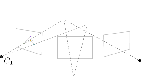
Figure 1: Illustrating the setup of equations (1) and (4).

Our practical contributions include implementing a numerical solver for full camera calibration, i.e., calibration of all $5$ unknown parameters of a perspective camera. We also consider common assumptions—namely, zero-skew and square pixels—and design fast solvers for specialized problems with a partially calibrated camera. These solvers can be fast enough for many online calibration applications, and can also bootstrap solutions using RanSaC-based frameworks with high accuracy in offline calibration settings. Among the strengths of our approach, we avoid well-known degeneracies of Kruppa’s equations [48] and recover $K$ directly instead of relying on estimates of the dual image of the absolute conic (DIAC), which may not be positive-semidefinite. Experiments show that our solvers outperform existing autocalibration methods in terms of accuracy in both synthetic and real image sequences despite increased runtime. Interfacing our solvers with COLMAP [44] further highlights the applicability of our approach.

Thus, our contribution is two-fold: i) theoretically, we provide a complete taxonomy of minimal autocalibration problems in $2$ or $3$ views; ii) practically, our novel solvers outperform classical autocalibration approaches in accuracy and are robust against degenerate configurations arising in very practical calibration scenarios when a camera revolves around an object, which is a substantial problem for all methods based on solving Kruppa’s equations [49].

1.2 Problem formulation

We recall here some standard constraints on the calibration matrix $K\in{\mathbb{R}}^{3\times 3}$ that involve the images of $N$ 3D points from $M$ different positions, as depicted in Figure 1. We want to estimate the entries of $K$: focal lengths $f$ and $g$, principal point $(u,v)$ and camera skew $s$. Image points are expressed in homogeneous coordinates $x_{ip}\in{\mathbb{R}}^{2}\times\{1\}$, i.e.,  $3\times 1$ vectors whose third entries equal $1$.

In Eq. (1) below and throughout the paper, the letter $i\in[M]:=\{1,\ldots M\}$ indexes a single image, while $p\in[N]:=\{1,\ldots,N\}$ indexes a point, ${}{R}_{i}\in{\mathbb{R}}^{3\times 3}$ denotes a rotation matrix, $C_{i}\in{\mathbb{R}}^{3}$ is a camera center, $X_{p}\in{\mathbb{R}}^{3}$ is a 3D point, and $\lambda_{ip}\in{\mathbb{R}}$ is the depth of the $p$-th point in the $i$-th camera [20].

Different flavors of the autocalibration problem exist in practice, depending on the available partial knowledge about the intrinsics in $K$. For instance, common assumptions are that the camera has square pixels ($f=g$) or zero skew ($s=0$). In general, we assume that there are $L$ linear equations $f_{1}(K)=\ldots=f_{L}(K)=0$ which encode any partial knowledge of intrinsics in $K$. For instance, if our camera has square pixels and no skew, then we may take $f_{1}(K)=s,$ $f_{2}(K)=f-g$.

Thus, assuming no noise in image points, a solution $K$ must satisfy the following conditions:

$$\small\lambda_{ip}\,x_{ip}=K\,R_{i}\left(\!\!\begin{array}[]{c}I\mid-C_{i}\end{array}\!\!\right)\left(\!\!\begin{array}[]{c}X_{p}\\ 1\end{array}\!\!\right),\ i\in[M],\ p\in[N],\\ {}{K}=\left(\!\!\begin{array}[]{ccc}f&s&u\\ 0&g&v\\ 0&0&1\end{array}\!\!\right),\begin{array}[]{cc}{}{R}_{i}^{\top}{}{R}_{i}={}{I},&\det{{}{R}_{i}}=1,\\[4.30554pt] \zeta_{ip}\lambda_{ip}=1,&\mu\,f\,g=1,\\[4.30554pt] f_{l}(K)=0,&l\in[L].\end{array}$$ (1)

The additional unknowns $\zeta_{ip}$ and corresponding equations $\zeta_{ip}\lambda_{ip}-1$ prohibit spurious solutions with zero depths. Similarly, $\mu\,f\,g-1=0$ ensures that $\det K=f\,g\neq 0$.

1.3 Previous work

We focus on the classical scenario where $K$ is constant across views. For work exploring the non-constant case, e.g., [38, 23] derive minimal conditions on the camera intrinsics for autocalibration. We also note that many works have addressed special cases of autocalibration, such as focal length estimation [41, 1, 46].

General methods fall roughly into two classes.

Direct methods use the so-called rigidity constraint encoded in fundamental matrices. In theory, $K$ can be recovered from the knowledge of three fundamental matrices resulting from three different camera motions [11, 34]. Direct methods [53, 19, 30] exploit this observation and recover the intrinsic parameters by solving Kruppa’s equations [28, 14]. Methods used to solve these equations vary considerably. In [30], instead of considering a complete, over-constrained system of $6$ equations in $5$ unknowns, a consensus solution is obtained by solving all $6$ of the square subsystems using a HC method. This work has several parallels to ours—namely, its use of HC solvers and the fact that these square subsystems are minimal relaxations in the sense of Section 3. The main difference is that their unknowns are the entries of the DIAC. In [53], the over-constrained system of Kruppa’s equations is solved with a nonlinear least squares technique; here, good initialization is needed to obtain an accurate estimate. We note that simplified polynomial systems have been derived by exploiting additional assumptions on $K$ [53]. Not all direct methods use Kruppa’s equations—in [33], a method analogous to the F4 method for computing Gröbner bases is devised for computing the DIAC. As our experiments illustrate, a common weakness of such direct approaches is that they do not enforce positive-semidefiniteness of the DIAC and hence fail with larger noise that makes the estimated DIAC indefinite.

Certain camera motions give rise to degenerate autocalibration problems [20, Ch. 19], [32], and additional degeneracies may exist for particular methods. For example, the method of [30] also falls short when the optical centers of all cameras lie on a sphere and the optical axes pass through the center of the sphere [49]. Although our approach employs a relaxation procedure analogous to this work, it does not suffer from the same degeneracy. Another limitation of direct methods is that they neglect non-trivial polynomial identities that tuples of compatible fundamental matrices must satisfy [20, 26, 15, 3].

Stratified methods assume that a projective reconstruction is known and stratify the problem into Affine and Euclidean stages. An affine reconstruction can be obtained by estimating the plane-at-infinity (PaI); from this, the assumption of constant $K$ allows its entries to be easily retrieved. This idea was pioneered in [21], where chirality constraints are used to estimate the location of the PaI. The PaI can also be located via the so-called modulus constraints. Specifically, in [39], this resulted in a system of three quartic polynomials on the coefficient of the PaI.

Rather than using the PaI, the work [51] directly encodes all metric information in terms of the absolute quadric, which, once retrieved, allows the intrinsic parameters to be retrieved by Cholesky factorization.

In general, stratified approaches are more robust to noise than direct ones but require good initialization of the PaI. Thus, some works [13, 4, 5] focus on optimality guarantees exploiting a branch-and-bound framework. Similarly, [17] samples the bounded space of intrinsic parameters to estimate the PaI robustly. Interestingly, [36] presents a branch-and-bound paradigm to solve direct and stratified autocalibration based on sampling algebraic varieties.

2 Our approach

We now outline our approach to autocalibration.

2.1 Depth equations and removing symmetries

In this work, we propose to eliminate camera extrinsics from (1) and use constraints involving the calibration matrix $K$ and depths $\lambda_{ip}$. By working with these constraints, we are able to avoid potential issues arising from fundamental matrix compatibility. This approach is also well-suited for constructing new minimal problems.

The main geometric constraint we use is that the Euclidean distance $\|X_{p}-X_{q}\|$ between any two 3D points $X_{p}$ and $X_{q}$ is the same whether these points are reconstructed from the $i$-th or the $j$-th camera, for any $i,j\in[M]$ as depicted in Fig. 1. Expressing each 3D point as $X_{p}=\lambda_{ip}K^{-1}x_{ip}$, this amounts to the vanishing of the function

$$\small d_{i,j,pq}(\lambda,K;x):= (\lambda_{ip}x_{ip}-\lambda_{iq}x_{iq})^{T}\omega(\lambda_{ip}x_{ip}-\lambda_{iq}x_{iq})$$

$$- (\lambda_{jp}x_{jp}-\lambda_{jq}x_{jq})^{T}\omega(\lambda_{jp}x_{jp}-\lambda_{jq}x_{jq}),$$

where $\omega=K^{-T}K^{-1}$ is the image of the absolute conic [20]. Note that $d_{i,j,pq}$ is a polynomial in $\lambda_{\bullet}$ and $x_{\bullet}$, and a rational function of $K$. We parametrize $\omega$ as

$$\small\omega=\begin{pmatrix}\frac{1}{{f^{\star}}}&-\frac{s^{\star}}{{f^{\star}}}&\frac{vs^{\star}-u}{f^{\star}}\\ -\frac{s^{\star}}{{f^{\star}}}&\frac{1}{g^{\star}}+\frac{{s^{\star}}^{2}}{f^{\star}}&\frac{us^{\star}-v{s^{\star}}^{2}}{f^{\star}}-\frac{v}{g^{\star}}\\ \frac{vs^{\star}-u}{f^{\star}}&\frac{us^{\star}-v{s^{\star}}^{2}}{f^{\star}}-\frac{v}{g^{\star}}&\frac{v^{2}}{g^{\star}}+\frac{(u^{2}-v^{2}{s^{\star}})^{2}}{f^{\star}}+1\end{pmatrix},$$ (2)

where $f^{\star}:=f^{2},\;\;g^{\star}:=g^{2},\;\;s^{\star}:=\frac{s}{g}.$ This parametrization is motivated by the invariance of $\omega$ under substitutions

$$\small f\to-f,\;\;\;(g,s)\to(-g,-s).$$ (3)

Thus, when $f,g$ and $s$ are unknown, solutions to the depth equations typically come in symmetric quadruples, and in pairs if only $f$ or $(g,s)$ are unknown. Substituting (2) into $d_{i,j,pq}$, we may rewrite our main constraint as

$$d_{i,j,pq}(\lambda,\omega;x)=0.$$ (4)

Depending on the minimal problem, (3) may not be the only symmetries present. For example, in the fully calibrated case $L=5,$ our minimal relaxation of four points in three views has $640$ solutions that can be grouped into pairs which differ only in the signs of depths in some view.

Remark: Our depth formulation can be viewed as a relaxation of the formulation (1). Thus, if we get a finite number of solutions, they surely give valid solutions to (1).

2.2 Specifying a minimal autocalibration problem

Instead of requiring that (4) holds for all $i,j\in[M],$ $p,q\in[N]$, we consider minimal problems which only require that a subset of these constraints hold. Hence, we will be in a situation similar to partial visibility as in [9, 27].

To specify a minimal problem, we consider:

(1) Priors on $K$: In practical situations, we often either possess or lack knowledge of intrinsics. When we know some intrinsics, we can transform images to normalize their known values to standard ones: $f=1,g=1,u=0,v=0,s=0$. Subsequently, we solve for the unknown transformed intrinsics and then recover their original values. We represent the knowledge of intrinsics as a 5-tuple of unknowns $\mathtt{fguvs}$. If any intrinsic is known, we replace its unknown with its normalized value. For instance, $\mathtt{f1uv0}$ indicates that $f,u,v$ are unknown, while $g=1$, $s=0$ are known. In the interesting scenario of a camera with square pixels, $\mathtt{ffuvs}$ encodes that $f$ and $g$ are unknown but equal.

(2) Number of cameras $M$: For a given 5-tuple $\mathtt{fguvs}$, we will see that the minimum number of cameras needed to obtain a minimal problem is either $2$ or $3$. Hence, we will investigate problems for only $2$ and $3$ cameras.

(3) Number of points $N$: For each five-tuple of intrinsics and $M$ cameras, we will consider the least number $N$ of points such that there is a set $\mathbf{g}$ of constraints in (4) providing a minimal problem.

(4) Constraints $\mathbf{g}$: For each triplet $(\mathtt{fguvs},M,N)$, we enumerate all possible subsets of constraints (4) which lead to different minimal problems.

Each four-tuple $(\mathtt{fguvs},M,N,\mathbf{g})$ specifies a candidate minimal problem [8]. Table 1 lists the 80 groups according to $(\mathtt{fguvs},M,N).$ For each group, we list the number $\#\mathbf{g}$ of equivalence classes of constraints leading to a minimal problem and a range of numbers of solutions in $\omega$.

Prior on $K$	$M$	$N$	$L$	Min # sol. in $\mathbb{C}$	Max # sol. in $\mathbb{C}$	# subsys.	$\#\mathbf{g}$	Prior on $K$	$M$	$N$	$L$	Min # sol. in $\mathbb{C}$	Max # sol. in $\mathbb{C}$	# subsys.	$\#\mathbf{g}$
$\mathtt{fguvs}$	2	-	0	$\infty$	$\infty$	0	0	$\mathtt{1g0vs}$	2	-	2	$\infty$	$\infty$	0	0
$\mathtt{fguvs}$	3	6	0	2985∗	1136202∗	5852925	3313	$\mathtt{1g0vs}$	3	5	2	29012	315653	1140	8
$\mathtt{fguv0}$	2	-	1	$\infty$	$\infty$	0	0	$\mathtt{1g0v0}$	2	7	3	18	18	1	1
$\mathtt{fguv0}$	3	5	1	2313	2313	190	3	$\mathtt{1g0v0}$	3	5	3	4400	102784	4845	37
$\mathtt{fgu0s}$	2	-	1	$\infty$	$\infty$	0	0	$\mathtt{1g00s}$	2	7	3	24	24	1	1
$\mathtt{fgu0s}$	3	5	1	2058	2058	190	3	$\mathtt{1g00s}$	3	5	3	4480	238544	4845	37
$\mathtt{fgu00}$	2	-	2	$\infty$	$\infty$	0	0	$\mathtt{1g000}$	2	6	4	30	30	1	1
$\mathtt{fgu00}$	3	5	2	9686	33606	1140	8	$\mathtt{1g000}$	3	4	4	668	668	1	1
$\mathtt{fg0vs}$	2	-	1	$\infty$	$\infty$	0	0	$\mathtt{11uvs}$	2	-	2	$\infty$	$\infty$	0	0
$\mathtt{fg0vs}$	3	5	1	2058	2058	190	3	$\mathtt{11uvs}$	3	5	2	57912	201265	1140	8
$\mathtt{fg0v0}$	2	-	2	$\infty$	$\infty$	0	0	$\mathtt{11uv0}$	2	7	3	48	48	1	1
$\mathtt{fg0v0}$	3	5	2	9686	112520	1140	8	$\mathtt{11uv0}$	3	5	3	8940	477080	4845	37
$\mathtt{fg00s}$	2	-	2	$\infty$	$\infty$	0	0	$\mathtt{11u0s}$	2	7	3	36	36	1	1
$\mathtt{fg00s}$	3	5	2	9686	33606	1140	8	$\mathtt{11u0s}$	3	5	3	8786	46192	4845	37
$\mathtt{fg000}$	2	7	3	18	18	1	1	$\mathtt{11u00}$	2	6	4	60	60	1	1
$\mathtt{fg000}$	3	5	3	3884	207664	4845	37	$\mathtt{11u00}$	3	4	4	1336	1336	1	1
$\mathtt{f1uvs}$	2	-	2	$\infty$	$\infty$	0	0	$\mathtt{110vs}$	2	7	3	72	72	1	1
$\mathtt{f1uvs}$	3	5	2	4111	4111	190	3	$\mathtt{110vs}$	3	5	3	16390	85480	4845	37
$\mathtt{f1uv0}$	2	-	2	$\infty$	$\infty$	0	0	$\mathtt{110v0}$	2	6	4	60	60	1	1
$\mathtt{f1uv0}$	3	5	2	29044	100816	1140	8	$\mathtt{110v0}$	3	4	4	1336	1336	1	1
$\mathtt{f1u0s}$	2	-	2	$\infty$	$\infty$	1	1	$\mathtt{1100s}$	2	6	4	60	60	1	1
$\mathtt{f1u0s}$	3	5	2	14760	160190	1140	8	$\mathtt{1100s}$	3	4	4	1336	1336	1	1
$\mathtt{f1u00}$	2	7	3	18	18	1	1	$\mathtt{11000}$	2	5	5	20	20	1	1
$\mathtt{f1u00}$	3	5	3	4400	244544	4845	37	$\mathtt{11000}$	3	4	5	640	640	1	1
$\mathtt{f10vs}$	2	-	2	$\infty$	$\infty$	0	0	$\mathtt{ffuvs}$	2	-	1	$\infty$	$\infty$	0	0
$\mathtt{f10vs}$	3	5	2	24332	86539	1140	8	$\mathtt{ffuvs}$	3	5	1	4617	4617	190	3
$\mathtt{f10v0}$	2	7	3	36	36	1	1	$\mathtt{ffuv0}$	2	-	2	$\infty$	$\infty$	0	0
$\mathtt{f10v0}$	3	5	3	7764	57220	4845	37	$\mathtt{ffuv0}$	3	5	2	16188	119119	1140	8
$\mathtt{f100s}$	2	7	3	18	18	1	1	$\mathtt{ffu0s}$	2	-	2	$\infty$	$\infty$	0	0
$\mathtt{f100s}$	3	5	3	4392	102778	4845	37	$\mathtt{ffu0s}$	3	5	2	29028	100758	1140	8
$\mathtt{f1000}$	2	6	4	30	30	1	1	$\mathtt{ffu00}$	2	7	3	24	24	1	1
$\mathtt{f1000}$	3	4	4	668	668	1	1	$\mathtt{ffu00}$	3	5	3	4484	176992	4845	37
$\mathtt{1guvs}$	2	-	1	$\infty$	$\infty$	0	0	$\mathtt{ff0vs}$	2	-	2	$\infty$	$\infty$	0	0
$\mathtt{1guvs}$	3	5	1	4360	4360	190	3	$\mathtt{ff0vs}$	3	5	2	38700	134352	1140	8
$\mathtt{1guv0}$	2	-	2	$\infty$	$\infty$	0	0	$\mathtt{ff0v0}$	2	7	3	24	24	1	1
$\mathtt{1guv0}$	3	5	2	29046	100808	1140	8	$\mathtt{ff0v0}$	3	5	3	4484	92336	4845	37
$\mathtt{1gu0s}$	2	-	2	$\infty$	$\infty$	0	0	$\mathtt{ff00s}$	2	7	3	36	36	1	1
$\mathtt{1gu0s}$	3	5	2	29024	100718	1140	8	$\mathtt{ff00s}$	3	5	3	7756	396042	4845	37
$\mathtt{1gu00}$	2	7	3	36	36	1	1	$\mathtt{ff000}$	2	6	4	30	30	1	1
$\mathtt{1gu00}$	3	5	3	7760	43315	4845	37	$\mathtt{ff000}$	3	4	4	668	668	1	1

Table 1: 80 groups of minimal autocalibration problems for $M\in\{2,3\}$ views. For each triplet $(\mathtt{fguvs},M,N)$ we list: i) $L$, the number of linear constraints on $K$, ii) the minimum and maximum solution count in $\mathbb{C}$, iii) $\#\text{subsys.}=\binom{(M-1)\binom{N}{2}}{M+N-L+4}$, the number of square subsystems of (4), iv) $\#\mathbf{g}$, the number of inequivalent minimal relaxations. The numbers $\#\mathbf{g}$ and $\textrm{Min }\#\textrm{ sol.}$ are most important, as they measure the number of minimal relaxations and the complexity of solving them. Solution counts refer to unknown depths and the parameters of $\omega$ in (2)–(4). The two counts $\bullet^{\ast}$ are only conjectural extrema, due to the prohibitive time needed to check all cases.

3 Relaxation, Enumeration, and Solving

We now give a more precise description of the taxonomy of minimal autocalibration problems presented in Table 1 and the tools needed to obtain it.

For each pair $(\mathtt{fguvs},M)$, we will determine whether camera calibration is possible and, if so, the minimum number $N$ of points such that there is a subset $\mathbf{g}$ of depth equations (4) providing a minimal problem. First, we determine the number of parameters among $\mathtt{fguvs}$ that can be estimated from $N$ 3D points seen in $M$ images captured by the same camera with constant $K$. Then, we determine the minimum number $N$ of 3D points required to solve the perspective autocalibration problem given a pair $(\mathtt{fguvs},M).$

Infeasible cases. In general, for $K$ unknown and non-constant, the reconstruction of $N$ 3D points from $M$ views can be obtained only up to a projective transformation $H$, which has $15$ degrees of freedom. Additional constraints on $H$ may allow us to assume $H$ is a similarity transformation with $7$ degrees of freedom. For $M=2$ views, the assumption that $K$ is constant puts $5$ constraints on $H.$ Thus, we need $L\geq 15-7-5=3$ linear constraints on $K$ to obtain a Euclidean reconstruction and hence recover the full $K$.

To determine the minimum number $N$ of 3D points required to solve the perspective camera autocalibration problem as a function of a pair $(\mathtt{fguvs},M)$, we must ensure that the number of degrees of freedom in image measurements is at least the number of degrees of freedom in the unknown scene and cameras. For this purpose, the full formulation (1) is preferable to the equations we actually use for solving, namely (4). This is because we can rigorously employ a count similar to that given in [8, §5]: we should assume there are at least

$$L\geq 3N+6M-2-2MN\vspace{-.5em}$$ (5)

independent linear constraints on $K$ in order to solve the autocalibration problem up to a finite number of candidate solutions. Noting also the trivial upper bound $L\leq 5,$ this explains the values of $L$ appearing in Table 1. The infeasible cases where $M=2$ and $L\leq 2$ have already been addressed above. The remaining cases are accounted for by (5) and the rows of Tab. 1. This table indicates that at least one minimal relaxation for the potentially feasible choices of $(M,N,L)$ actually exists. To properly interpret the table, we must now formalize what we mean when we say a subsystem $\mathbf{g}$ of equations determines a minimal relaxation of the autocalibration problem (1).

3.1 Minimal problems and minimal relaxations

Many estimation problems in vision can be expressed using the language of algebraic geometry. In general, we may consider an irreducible algebraic variety $X$, whose points consist of problem-solution pairs $(\mathbf{p},\mathbf{x})\in{\mathbb{C}}^{m}\times{\mathbb{C}}^{n}$ satisfying some set of equations depending polynomially on $\mathbf{p}$ and $\mathbf{x}$. Our task is to estimate the solution $\mathbf{x}\in{\mathbb{C}}^{n}$ given some problem instance $\mathbf{p}\in{\mathbb{C}}^{m},$ meaning $(\mathbf{p},\mathbf{x})\in X.$

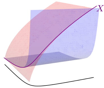
Figure 2: Minimal relaxations $\mathbb{V}(\mathbf{g}_{1})$, $\mathbb{V}(\mathbf{g}_{2})$, w/ $X=\mathbb{V}(\mathbf{g}_{1},\mathbf{g}_{2})$, $\mathbf{g}_{1}(p_{1},p_{2},x)=x^{2}-p_{1}$, and $\mathbf{g}_{2}(p_{1},p_{2},x)=p_{2}x^{2}-1.$

More specifically, image points $\mathbf{p}=(x_{ip})_{i\in[M],p\in[N]}$ specify an instance of an autocalibration problem. We want to estimate the unknowns $\mathbf{x}$ defining $\omega$ in (2) and the (suitably normalized) depths $(\lambda_{ip}).$ Thus $m=2MN$ and $n=(5-L)+MN-1.$ If we define the variety $X$ to be the image of a rational map (much like the joint camera map of [8, §4]), the condition that $X$ is irreducible holds.

Let $\pi$ denote the map which projects $X$ into the space of problem instances ${\mathbb{C}}^{m}$, i.e.,

$$\pi:X\to{\mathbb{C}}^{m},\quad(\mathbf{p},\mathbf{x})\mapsto\mathbf{p}.\vspace{-.5em}$$ (6)

The set of solutions of some problem instance $\mathbf{p}\in{\mathbb{C}}^{m}$ may be identified with the fiber $\pi^{-1}(\mathbf{p})$. Following [8], we say that $\pi$ defines a minimal problem if the following hold:

1. The problem is balanced—that is, $\dim X=m.$

2. Almost every problem instance in ${\mathbb{C}}^{m}$ has a solution—equivalently, the image of the map $\pi$ is dense in ${\mathbb{C}}^{m}.$

In practice, we check that a problem is minimal using some system of equations $\mathbf{g}(\mathbf{p},\mathbf{x})=0$ defining $X$ locally, via the following rank conditions at a point $(\mathbf{p}_{0},\mathbf{x}_{0})\in X$:

$$\small\operatorname{rank}\left(\frac{\partial\mathbf{g}}{\partial\mathbf{p}}\mid\frac{\partial\mathbf{g}}{\partial\mathbf{x}}\right)\Big{|}_{(\mathbf{p}_{0},\mathbf{x}_{0})}=\operatorname{rank}\left(\frac{\partial\mathbf{g}}{\partial\mathbf{x}}\right)\Big{|}_{(\mathbf{p}_{0},\mathbf{x}_{0})}=n.\vspace{-.5em}$$ (7)

Some of the cases appearing in Table 1 are already minimal problems. These are precisely the rows where both sides of (5) are equal. In general, $\dim X=3N+6M-2-L.$

When the inequality (5) is strict, we expect the autocalibration problem (1) to be overconstrained in the sense that a generic problem in ${\mathbb{C}}^{m}$ does not have an exact solution.

To deal with overconstrained problems, consider a system $\mathbf{g}$ consisting of $n$ polynomial or rational functions vanishing on $X$—that is, $X\subset\mathbb{V}(\mathbf{g})$ where

$$\small\mathbb{V}(\mathbf{g})=\overline{\{(\mathbf{p},\mathbf{x})\in{\mathbb{C}}^{m+n}\mid\mathbf{g}(\mathbf{p},\mathbf{x})\text{ is defined and equals }0\}}$$

($\overline{\,\cdot\,}$ denotes the Zariski closure [6, §4.4].) If the rank conditions (7) hold at a generic point $(\mathbf{p}_{0},\mathbf{x}_{0})\in X,$ we say that $\mathbf{g}$ determines a minimal relaxation of $\pi$. Figure 2 illustrates this definition on a simple example (see SM 9 for details).

In general, an overconstrained problem can have different minimal relaxations. In the next section, we obtain a combinatorial classification of all minimal relaxations obtained from subsets of the depth constraints (4), grouping minimal relaxations into natural equivalence classes.

3.2 Enumerating Minimal Relaxations

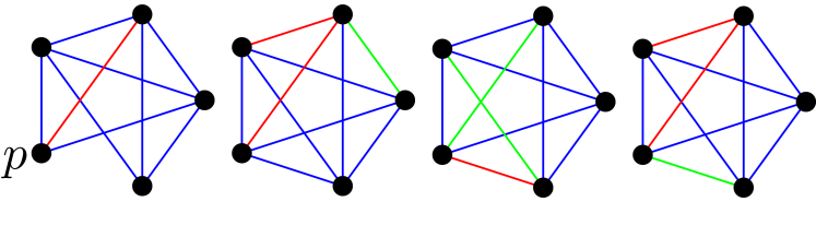
Figure 3: Non-isomorphic 4-colorings when $L=2$ in 3 views. 3D point pairs $(p,q)$ are colored according to the removal of depth equations $d_{i,j,pq}$ in the relaxed subsystem. $W$ (white) indicates removal from both image pairs, ${\color[rgb]{0,0,1}B}$ no removal. ${\color[rgb]{1,0,0}R}$ and ${\color[rgb]{0,1,0}G}$ indicate removal in image pairs (1,3) and (1,2), respectively.

We now explain how to obtain minimal relaxations of autocalibration problems using the depth equations (4). The combinatorial structure of minimal relaxations obtained by removing a subset of equations (4) is neatly encoded by a 4-coloring: that is, a function $c\colon\binom{[N]}{2}\to\{{\color[rgb]{0,0,1}B},{\color[rgb]{1,0,0}R},{\color[rgb]{0,1,0}G},W\}$, which assigns one of four colors to all pairs of 3D points. In standard graph-theoretic terminology, these are exactly the improper edge 4-colorings of the complete graph $K_{N}.$ Every 4-coloring determines a subsystem of equations (4)—for each edge $pq\in\binom{[N]}{2},$ we take equations $\mathbf{g}$ in the set

$$\small\{d_{1,2,pq}\mid c(pq)\in\{{\color[rgb]{0,0,1}B},{\color[rgb]{1,0,0}R}\}\}\cup\{d_{1,3,pq}\mid c(pq)\in\{{\color[rgb]{0,0,1}B},{\color[rgb]{0,1,0}G}\}\}.$$ (8)

We say two 4-colorings $c_{1},c_{2}:\binom{[N]}{2}\to\{{\color[rgb]{0,0,1}B},{\color[rgb]{1,0,0}R},{\color[rgb]{0,1,0}G},W\}$ are isomorphic if there exist permutations $\sigma:[N]\to[N]$ and $\tau:\{{\color[rgb]{0,0,1}B},{\color[rgb]{1,0,0}R},{\color[rgb]{0,1,0}G},W\}\to\{{\color[rgb]{0,0,1}B},{\color[rgb]{1,0,0}R},{\color[rgb]{0,1,0}G},W\}$ such that $\tau(W)=W,$ $\tau({\color[rgb]{0,0,1}B})={\color[rgb]{0,0,1}B},$ and $c_{2}=\tau\circ c_{1}\circ\sigma.$ The minimal relaxations determined by isomorphic 4-colorings are equivalent, since $\tau$ corresponds to swapping views $2$ and $3,$ and $\sigma$ corresponds to relabeling world points. Fig. 3 shows an example.

Determining isomorphism classes of 4-colorings, i.e., and thus equivalence classes of minimal relaxations $\mathbf{g}$, offers us a key practical advantage. Given the large number of 4-colorings, exceeding 5 million for $\mathtt{fguvs}$, computing the solution count for all associated problems is computationally prohibitive. Consequently, we opt to consider only one representative per isomorphism class when computing solutions offline with HC. This approach facilitates the creation of the comprehensive taxonomy outlined in Tab. 1. We determine a unique representative $c$ in each isomorphism class using the line graph $\mathcal{L}(c)$, as detailed in 10 of the SM.

3.3 Solving with homotopy continuation

For any system $\mathbf{g}(\mathbf{p},\mathbf{x})=0$ encoding a minimal relaxation of an autocalibration problem, we construct minimal solvers using a standard online/offline approach based on numerical HC methods. In the offline stage, we construct a synthetic solution $(\mathbf{p}_{0},\mathbf{x}_{0})\in X\supset X_{\mathbf{g}}$ by fabricating a 3D scene. If $\mathbf{g}$ arises from a balanced problem, we check that it is minimal via the rank conditions (7), and use monodromy heuristics [7] to recover (with high probability) all remaining solutions in $\pi^{-1}(\mathbf{p}_{0},\mathbf{x}_{0})$ for the synthetic parameters $\mathbf{p}_{0}\in{\mathbb{C}}^{m}$. As postprocessing, we use parameter homotopy [45, Ch. 8] with equations $\mathbf{g}$ to track all solutions to new parameter values $\mathbf{p}_{1}\in{\mathbb{C}}^{m}$ whose coordinates are random complex numbers. Finally, in the online stage, the solver receives a new problem instance $\mathbf{p}_{2}\in{\mathbb{R}}^{m}$ as input, and uses parameter homotopy to track all solutions for $\mathbf{p}_{1}$ to those for $\mathbf{p}_{2}.$

4 Experiments

We evaluate the performance of our proposed minimal solvers on simulated and real image sequences, with a focus on three of the most practical cases: i) $\mathtt{ffuv0}$, an uncalibrated camera with square pixel aspect ratio and zero-skew, ii) $\mathtt{fguv0}$, an uncalibrated camera with zero-skew, iii) $\mathtt{fguvs}$, a fully uncalibrated camera. First, we assess the theoretical correctness of our proposed solvers and their resilience to noise in simulated image sequences (Sec. 4.1). Then, in Sec. 4.2, we perform experiments on real image sequences and compare the results attained by our solvers with several competing autocalibration methods. Finally, we demonstrate that integrating our solvers into the reconstruction pipeline COLMAP [43, 44] improves autocalibration and reconstruction on real image sequences (Sec. 4.3).

Competitors. We compare our solvers to the HC-based method for solving Kruppa’s equations in [30]. As described in Sec. 1.3, we remark that, in this method, each subsystem of $5$ / $6$ Kruppa’s equations may also be considered minimal relaxations in the sense of Section 3. Moreover, whether we consider these equations as rational or polynomial functions matters. In the latter case, considered in [30], it was correctly observed that these equations had the expected number of $2^{5}=32$ solutions over ${\mathbb{C}}.$ However, for $14$ of these solutions, denominators appearing in the rational form of Kruppa’s equations become undefined. Thus, only 18 HC paths must be tracked to find a valid solution.

To address the imbalance between our method (based on triples of image points) and Kruppa (based on triples of fundamental matrices), we consider three variants of Kruppa that estimate these fundamental matrices differently. The first variant, Kruppa-8, estimates fundamental matrices using the non-minimal 8-point algorithm. The second, Kruppa-7, estimates fundamental matrices using the minimal 7-point algorithm. The third, Kruppa-6, implements a minimal solver for projective reconstruction from 6 points in 3 views [42], from which a set of compatible fundamental matrices can be determined. Kruppa-6 is the closest to our $\mathtt{fguvs}$ solver, which also requires six points. For all three variants, we normalize the input as in [22].

In real-world experiments, we also compare our solvers with the state-of-the-art camera autocalibration approach presented in [36]. This method uses semidefinite programming and a Branch-and-Bound (BnB) scheme to maximize consensus among polynomials and solve the calibration problem with either the Kruppa equations [31] or the modulus constraint [37]. We refer to these variants as Kruppa BnB and Modulus BnB, respectively.

Implementation. We implement our solvers in Julia using the package HomotopyContinuation [2], with C++ and Python bindings. SM 11.1 reports the minimal relaxations used by these solvers. All experiments were conducted on an Intel Core i9 13900k with 16GB RAM.

4.1 Synthetic Experiments

Figure 4: Autocalibration Evaluation on Synthetic Images. Solver accuracy is assessed under varying levels of zero-mean Gaussian noise (denoted by $\sigma$ on the x-axis) applied to pixel coordinates. Mean reprojection error and relative errors in focal lengths $\Delta fg$, principal point $\Delta uv$, and skew $\Delta s$ are reported. For error measures, boxes represent the interquartile range of error distribution. The right-most plot illustrates the failure rate as a percentage, with $\mathtt{ffuv0}$, $\mathtt{fguv0}$, and $\mathtt{fguvs}$ excluded due to no failures.

We evaluate the performance of our $\mathtt{ffuv0}$, $\mathtt{fguv0}$, and $\mathtt{fguvs}$ solvers in synthetic images under varying noise levels applied to the generated pixel coordinates. Our evaluation involves comparing the Kruppa-8 [30] and Kruppa-6 methods. Results for Kruppa-7 are inferior in accuracy and are presented in SM 11.4.

Simulations. In each simulated scene, we generate 100 randomly distributed 3D points within the unit sphere. We simulate three camera displacements, with the first located 2 world units from the sphere’s center along the y-axis. The other two cameras are translated by $\pm 0.5$ units along all axes relative to the first camera, enforcing a minimum L2-norm of $0.1$ for translation vectors. Camera motion is constrained to ensure all views capture the scene, with random rotations obtained by uniformly sampling angles in the $\pm 45$ degrees range along all axes. Simulated points are projected onto $640\times 480$ images, discarding any points not observed in all views. Noise is introduced by adding zero-mean Gaussian displacements to pixel coordinates with standard deviation $\sigma$ in the $[0,1]$ range in increments of 0.2. For each noise level $\sigma$, we conduct 1000 independent tests for all methods. Our solvers, Kruppa-6 and Kruppa-8 [30] are evaluated with intrinsics: $f=330$, $g=310$, $u=300$, $v=250$, $s=10$.

Metrics. We report the relative error $\Delta fg$ in focal lengths and errors in the principal point $\Delta uv$ and skew $\Delta s$,

$$\small\Delta uv=\frac{1}{2}\left(\frac{\left|\hat{u}-u_{\mathrm{gt}}\right|}{u_{\mathrm{gt}}}+\frac{\left|\hat{v}-v_{\mathrm{gt}}\right|}{v_{\mathrm{gt}}}\right),\quad\Delta s=2\frac{\left|\hat{s}-s_{\mathrm{gt}}\right|}{f_{\mathrm{gt}}+g_{\mathrm{gt}}}.$$

We report the reprojection error $Re$ computed using the estimated intrinsics $K$ and camera poses $\{R_{i},C_{i}\}_{i=1}^{M}$. Note that $Re$ is not reported for Kruppa-8 due to the inconsistent reconstruction across the three views obtained from fundamental matrices computed using the 8-point algorithm. This inconsistency leads to significantly higher errors, making any comparison unfair. Instead, we report $Re$ for Kruppa-6, where a metric reconstruction consistent across the three views is obtained by upgrading the projective cameras using the estimated intrinsic parameters.

Results. In Fig. 4, boxes represent the interquartile range of errors in estimated camera parameters and mean reprojection error. Errors generally increase with higher noise levels $\sigma$. Across most experiments, $\mathtt{ffuv0}$ and $\mathtt{fguv0}$, despite assuming prior camera knowledge not aligned to the synthetic camera parameters, match or surpass Kruppa methods, particularly in focal length, with principal point results generally within a $\pm 5\%$ deviation from Kruppa methods. $\mathtt{fguvs}$, similar to Kruppa’s in not assuming prior camera knowledge, attains comparable performance to Kruppa methods in focal length and principal point estimation but underperforms in skew estimation, especially for $\sigma>0.4$. Across all noise levels, all our solvers outperform Kruppa-6 in reprojection error, which jointly assesses the accuracy in intrinsic camera parameters and camera pose estimation.

Kruppa methods recover $K$ via the Cholesky decomposition of the DIAC $\omega^{\ast}$. In the presence of noise, $\omega^{\ast}$ may not be positive-semidefinite. This leads to autocalibration failure, making the estimation of $K$ unfeasible. Failure rates range from $4\%$ to $13\%$ for Kruppa-6 and from $3\%$ to $6\%$ for Kruppa-8, as reported in Fig. 4-right. In principle, our solvers could also fail at higher noise levels. However, we did not encounter these issues in our synthetic experiments.

Remark 1. In SM 11.4, we confirm the theoretical correctness of $\mathtt{ffuv0}$ and $\mathtt{fguv0}$ by showing that zero error is attained in the noiseless case when each solver’s prior camera knowledge matches the synthetic camera parameters.

Remark 2. All Kruppa-based methods present a degeneracy arising from a singularity in the Kruppa equations when the optical centers of cameras lie on a sphere, and their optical axes intersect at the sphere’s center [49]. As discussed in SM 11.4, we reproduce such conditions and confirm that our method is unaffected by the Kruppa degeneracy.

4.2 Evaluation on Real Datasets

	Fountain-P11							Herz-Jesu-P8
Method	$\Delta fg$	$\Delta uv$	$\Delta s$	$Re_{\mathrm{gt}}$	$Re$	$\epsilon_{R}$	$\epsilon_{C}$	$\Delta fg$	$\Delta uv$	$\Delta s$	$Re_{\mathrm{gt}}$	$Re$	$\epsilon_{R}$	$\epsilon_{C}$
Kruppa-6	0.137	0.184	0.022	19.563	2.891	7.061	5.579	0.098	0.112	0.014	14.565	1.112	2.125	1.902
Kruppa-7	0.249	0.204	0.040	28.197	-	-	-	0.122	0.114	0.040	15.252	-	-	-
Kruppa-8 [30]	0.260	0.173	0.029	28.466	-	-	-	0.140	0.115	0.022	13.606	-	-	-
Kruppa BnB [36]	0.127	0.058	0.014	9.231	-	-	-	0.078	0.096	0.018	21.023	-	-	-
Modulus BnB [36]	0.162	0.071	0.016	10.540	-	-	-	0.097	0.102	0.019	22.641	-	-	-
$\mathtt{ffuv0}$	0.017	0.029	-	4.435	0.449	0.623	0.664	0.017	0.044	-	8.082	0.672	0.664	0.656
$\mathtt{fguv0}$	0.028	0.050	-	8.580	0.554	0.970	1.183	0.029	0.063	-	11.128	0.680	1.295	1.540
$\mathtt{fguvs}$	0.035	0.064	0.008	9.769	1.075	1.274	1.428	0.041	0.058	0.013	11.348	0.989	1.085	1.139

Table 2: Autocalibration Evaluation on Real Datasets. Mean relative errors in the focal lengths $\Delta fg$, principal point $\Delta uv$, and skew $\Delta s$ are reported. Reprojection error is computed in two variations: i) $Re_{\mathrm{gt}}$, using estimated $K$ and ground truth camera poses, ii) $Re$, using estimated $K$ and estimated camera poses (when applicable). $\epsilon_{R}$ and $\epsilon_{C}$ are the angular errors in estimated camera rotations and translations, respectively. Lower values indicate better performance for all metrics.

	Fountain-P11				Rathaus				KITTI-Depth
Variant	$\Delta fg\downarrow$	$\Delta uv\downarrow$	$Re$	Points3D	$\Delta fg\downarrow$	$\Delta uv\downarrow$	$Re$	Points3D	$\Delta fg\downarrow$	$\Delta uv\downarrow$	$Re$	Points3D
$\text{COLMAP}_{\mathrm{guess}}$	0.3350	0.0140	0.444	4848	0.0671	0.0812	0.624	847	0.6510	0.1360	0.810	210
$\text{COLMAP}_{\texttt{fguv0}}$	0.0058	0.0297	0.241	5356	0.0237	0.0111	0.450	823	0.0720	0.0185	0.409	231
$\text{COLMAP}_{\mathrm{guess}}$ + $K\text{-BA}$	0.0012	0.0013	0.212	5296	0.0185	0.0607	0.435	868	0.3480	0.5072	0.547	232
$\text{COLMAP}_{\texttt{fguv0}}$ + $K\text{-BA}$	0.0011	0.0012	0.212	5367	0.0165	0.0307	0.432	823	0.0626	0.1773	0.404	236
$\text{COLMAP}_{\mathrm{gt}}$ + $K\text{-BA}$	0.0013	0.0011	0.210	5368	0.0069	0.0291	0.430	794	0.0401	0.0553	0.398	237

Table 3: Comparing errors and numbers of registered points for autocalibration strategies in COLMAP (Sec. 4.3.)

We assess autocalibration accuracy on the calibrated Fountain-P11 and Herz-Jesu-P8 [47] datasets. The $\mathtt{ffuv0}$, $\mathtt{fguv0}$, and $\mathtt{fguvs}$ solvers are embedded in a conventional MSaC-framework [50]. At each iteration of the MSaC, we evaluate the recovered camera intrinsics and extrinsics in terms of their induced reprojection error weighted by the Huber loss. We set a limit of 200 iterations. Image points are obtained by extracting and matching SIFT [29] keypoints across image triplets.

We compare our solvers with Kruppa-8 [30], Kruppa-7, and Kruppa-6 embedded in MSaC, mirroring our solver setup. For Kruppa-8 and Kruppa-7, we compute camera poses by decomposing the pairwise essential matrices $E=K^{\top}FK=[t]_{\times}R$, where $F$ is the fundamental matrix. Then, we compute the reprojection error pairwise, averaging it across all image pairs. Kruppa-6 yields a consistent metric reconstruction across the three views, allowing direct computation of the reprojection error by projecting the 3D points using the recovered camera matrices. Finally, our evaluation includes Kruppa BnB and Modulus BnB [36], representing state-of-the-art autocalibration methods.

Metrics. We assess calibration accuracy using $\Delta fg$, $\Delta uv$, $\Delta s$ in Sec. 4.1. We also report reprojection errors $Re$, computed using estimated camera intrinsics and extrinsics, and $Re_{\mathrm{gt}}$, computed using the estimated intrinsics, but ground truth camera poses. $\epsilon_{R}$ and $\epsilon_{C}$ represent the angular errors in degrees for estimated camera rotations and centers, respectively. Errors are averaged across all image sequences.

Results. Tab. 2 reports the results of our evaluation. Concerning full camera calibration, our $\mathtt{fguvs}$ solver sets the benchmark for most calibration metrics, except for $\Delta uv$ in Fountain-P11, where it is the second-best method after Kruppa BnB. $\mathtt{fguvs}$ also outperforms Kruppa-6 at camera pose estimation. Remarkably, $\mathtt{fguvs}$ excels in focal length estimation, achieving 3.6 times lower $\Delta fg$ in Fountain-P11 compared to the second-best Kruppa BnB.
The solvers $\mathtt{ffuv0}$ and $\mathtt{fguv0}$ outperform $\mathtt{fguvs}$ across various metrics, with $\mathtt{ffuv0}$ emerging as the top-performing method overall. This demonstrates the advantages of integrating partial knowledge of $K$ into our solvers, especially given that the zero-skew assumption and square pixel aspect ratio very often hold in practice.
Our solvers’ runtimes depend on the number of paths tracked by HC, i.e., by the solution counts in $\mathbb{C}$. We refer to Tab. 1 to optimize speed and select $\mathbf{g}$ with the lowest solution count. We report the median runtime per iteration: $\mathtt{fguv0}$ 1.78 s/iter (2313 paths), $\mathtt{fguvs}$ 2.15 s/iter (2985 paths), $\mathtt{ffuv0}$ 9.21 s/iter (16188 paths). Our solvers are multithreaded, with quasi-linear scaling in the number of CPU cores. Comparatively, the median runtime for Kruppa-6, Kruppa-7, and Kruppa-8 is 0.71 s/iter, with $6\cdot 18=108$ solutions paths overall. For Kruppa, we observe that performance scaling is not linear, but we attribute this to the small number of solutions and overhead when running the Julia HC solver. Despite their faster runtimes, these methods exhibit inferior accuracy and higher failure rates, as illustrated in Fig. 4. Setting a strict threshold of 0.02 on $\Delta fg$, the $\mathtt{fguvs}$ solver takes an average of 4.21 minutes on Fountain-P11 and Herz-Jesu-P8, whereas Kruppa methods are, on average, only 27% faster. The BnB methods [36] are the fastest overall, by 62% compared to ours, yet they still provide inferior accuracy.

4.3 Autocalibration in COLMAP

We integrate our autocalibration solvers into COLMAP [43, 44] to initialize the camera intrinsics before 3D reconstruction. The evaluation is conducted on five triplets of images from the Fountain-P11 (2 sequences), Rathaus [47] (1 sequence), and KITTI-Depth [16] (2 sequences) datasets. We report results for $\mathtt{fguv0}$. Additional details about other solvers and datasets may be found in SM 11.
We consider two strategies for initializing $K$: $\text{COLMAP}_{\mathrm{guess}}$ uses the default COLMAP guess based on image size, and $\text{COLMAP}_{\mathtt{fguv0}}$ employs the $\mathtt{fguv0}$ solver. These variants exclude the $K$ from Bundle Adjustment (BA). We also evaluate results obtained using BA on $K$ (+ $K\text{-BA}$). $\text{COLMAP}_{\mathrm{gt}}$ + BA involves starting from ground truth camera parameters and applying BA and is provided as an oracle for performance.
Tab. 3 reports results for each strategy. $\text{COLMAP}_{\mathtt{fguv0}}$ estimates $K$ better than $\text{COLMAP}_{\mathrm{guess}}$ in most cases and yields accurate reconstructions, even without refining $K$. When applying BA, the gap between $\text{COLMAP}_{\mathtt{fguv0}}$ and $\text{COLMAP}_{\mathrm{guess}}$ narrows, particularly in Fountain-P11, where many keypoints are available. In Rathaus, the principal point is displaced from the image center. The final calibration accuracy is improved by using the estimate of $K$ from $\mathtt{fguv0}$. In KITTI-Depth, BA often struggles due to fewer matches. In this scenario, using BA results in a 9.58x degradation in $\Delta uv$, but only a 1.15x improvement in $\Delta fg$ compared to the calibration by $\mathtt{fguv0}$. This indicates that in challenging scenes, our estimates of $K$ are more reliable than those obtained solely through refinement with BA.

5 Conclusion

Motivated by the quest for a complete understanding of the autocalibration of a camera with constant $K$, we presented a new complete analysis of minimal autocalibration problems and their implementations, improving the state-of-the-art.

Acknowledgements: TD was supported by NSF DMS-2103310. APDC and LM were supported by FAIR (Future Artificial Intelligence Research) project funded by the NextGenerationEU program within the PNRR-PE-AI scheme (M4C2, Investment 1.3, Line on Artificial Intelligence) and by GEOPRIDE ID: 2022245ZYB, CUP: D53D23008370001, (PRIN 2022 M4.C2.1.1 Investment). EU H2020 No. 871245 SPRING project supported TP.

In this document, we provide additional details concerning the main paper.

6 Problem formulation — additional details

Although the depth equations (4) described in Sec. 2.1 are the main constraints used in our approach, we wish to point out that they are by no means the only polynomial equations involving depths $\lambda_{ip},$ image points $x_{ip}$ and the calibration matrix $K$ that must be satisfied by an exact solution $((\lambda_{ip}),K).$ In the language of Sec. 11.1: the depth constraints determine the variety of problem-solution pairs $X$ locally but not globally.

We may derive additional constraints as follows: using (1), for any view pair $1\leq i<j\leq M$ and four distinct world points with indices $1\leq p_{1},\ldots,p_{4}\leq 4$, we have

$$\det\left(\begin{smallmatrix}\lambda_{ip_{1}}x_{ip_{1}}-\lambda_{ip_{2}}x_{ip_{2}}&\lambda_{ip_{3}}x_{ip_{3}}-\lambda_{ip_{2}}x_{ip_{2}}&\lambda_{ip_{4}}x_{ip_{4}}-\lambda_{ip_{2}}x_{ip_{2}}\end{smallmatrix}\right)=$$

$$\det\left(\begin{smallmatrix}\lambda_{jp_{1}}x_{jp_{1}}-\lambda_{jp_{2}}x_{jp_{2}}&\lambda_{jp_{3}}x_{jp_{3}}-\lambda_{jp_{2}}x_{jp_{2}}&\lambda_{jp_{4}}x_{jp_{4}}-\lambda_{jp_{2}}x_{jp_{2}}\end{smallmatrix}\right).$$ (9)

This follows from our assumption that $K$, and hence also $\det(K)$, is constant: compare with (19) below.

It is important to remember that, when solving with a minimal relaxation, the equations that are not enforced may or may not continue to hold for noisy data. As an example of this, we may consider the unique class of minimal problems in Table 1 for the scenario $\mathtt{11000}$ with $M=3$ fully calibrated views. As illustrated in Fig. 5, we may drop exactly one depth equation for the view pair $(i,j)=(1,2)$ to obtain a representative for the equivalence class of minimal relaxations. This relaxation has the effect that (9) no longer must hold for this view pair. Indeed, we find that this equation is typically violated in the case of noisy data and for all $639$ non-synthetic solutions when solving a generic synthetic problem instance. On the other hand, for the view pair $(i,j)=(1,3)$, the equation (9) holds even for non-synthetic solutions or noisy data.

We may rephrase the observations of the previous paragraph in the geometric language developed in Sec. 3 (see also SM 9 below.) From this point of view, (9) is valid for both view pairs on the incidence variety $X$ associated with the overconstrained problem but only generally valid for the view pair $(1,3)$ on the incidence variety $\mathbb{V}(\mathbf{g})$ associated to the minimal relaxation. The local nature of parameter homotopy ensures, for this problem, that we do not need to explicitly enforce the constraint (9) for one view pair. However, any attempt to simultaneously enforce these constraints for both view pairs and the chosen depth constraints will invariably lead us back to an overconstrained problem.

Figure 5: Visualization of a representative of the equivalence class of minimal relaxations for the $\mathtt{11000}$ problem obtained by dropping a constraint $d_{1,2,pq}$ for view pair $(1,2)$.

Prior on $K$	$M$	$N$	$L$	Min # sol. in $\mathbb{C}$	Max # sol. in $\mathbb{C}$	$\#\text{balanced}$	$\#\mathbf{g}$	Prior on $K$	$M$	$N$	$L$	Min # sol. in $\mathbb{C}$	Max # sol. in $\mathbb{C}$	$\#\text{balanced}$	$\#\mathbf{g}$
$\mathtt{fguvs}$	2	-	0	$\infty$	$\infty$	0	0	$\mathtt{1g0vs}$	2	-	2	$\infty$	$\infty$	0	0
$\mathtt{fguvs}$	3	6	0	$11940^{\ast}$	$4544808^{\ast}$	5852925	3313	$\mathtt{1g0vs}$	3	5	2	58024	631306	1140	8
$\mathtt{fguv0}$	2	-	1	$\infty$	$\infty$	0	0	$\mathtt{1g0v0}$	2	7	3	36	36	1	1
$\mathtt{fguv0}$	3	5	1	9252	9252	190	3	$\mathtt{1g0v0}$	3	5	3	8800	205568	4845	37
$\mathtt{fgu0s}$	2	-	1	$\infty$	$\infty$	0	0	$\mathtt{1g00s}$	2	7	3	48	48	1	1
$\mathtt{fgu0s}$	3	5	1	8232	8232	190	3	$\mathtt{1g00s}$	3	5	3	8960	477088	4845	37
$\mathtt{fgu00}$	2	-	2	$\infty$	$\infty$	0	0	$\mathtt{1g000}$	2	6	4	60	60	1	1
$\mathtt{fgu00}$	3	5	2	38744	134424	1140	8	$\mathtt{1g000}$	3	4	4	1336	1336	1	1
$\mathtt{fg0vs}$	2	-	1	$\infty$	$\infty$	0	0	$\mathtt{11uvs}$	2	-	2	$\infty$	$\infty$	0	0
$\mathtt{fg0vs}$	3	5	1	8232	8232	190	3	$\mathtt{11uvs}$	3	5	2	57912	201265	1140	8
$\mathtt{fg0v0}$	2	-	2	$\infty$	$\infty$	0	0	$\mathtt{11uv0}$	2	7	3	48	48	1	1
$\mathtt{fg0v0}$	3	5	2	38744	450080	1140	8	$\mathtt{11uv0}$	3	5	3	8940	477080	4845	37
$\mathtt{fg00s}$	2	-	2	$\infty$	$\infty$	0	0	$\mathtt{11u0s}$	2	7	3	36	36	1	1
$\mathtt{fg00s}$	3	5	2	38744	134424	1140	8	$\mathtt{11u0s}$	3	5	3	8786	46192	4845	37
$\mathtt{fg000}$	2	7	3	72	72	1	1	$\mathtt{11u00}$	2	6	4	60	60	1	1
$\mathtt{fg000}$	3	5	3	15536	830656	4845	37	$\mathtt{11u00}$	3	4	4	1336	1336	1	1
$\mathtt{f1uvs}$	2	-	2	$\infty$	$\infty$	0	0	$\mathtt{110vs}$	2	7	3	72	72	1	1
$\mathtt{f1uvs}$	3	5	2	8222	8222	190	3	$\mathtt{110vs}$	3	5	3	16390	85480	4845	37
$\mathtt{f1uv0}$	2	-	2	$\infty$	$\infty$	0	0	$\mathtt{110v0}$	2	6	4	60	60	1	1
$\mathtt{f1uv0}$	3	5	2	58088	201632	1140	8	$\mathtt{110v0}$	3	4	4	1336	1336	1	1
$\mathtt{f1u0s}$	2	-	2	$\infty$	$\infty$	1	1	$\mathtt{1100s}$	2	6	4	60	60	1	1
$\mathtt{f1u0s}$	3	5	2	29520	320380	1140	8	$\mathtt{1100s}$	3	4	4	1336	1336	1	1
$\mathtt{f1u00}$	2	7	3	36	36	1	1	$\mathtt{11000}$	2	5	5	20	20	1	1
$\mathtt{f1u00}$	3	5	3	8800	489088	4845	37	$\mathtt{11000}$	3	4	5	640	640	1	1
$\mathtt{f10vs}$	2	-	2	$\infty$	$\infty$	0	0	$\mathtt{ffuvs}$	2	-	1	$\infty$	$\infty$	0	0
$\mathtt{f10vs}$	3	5	2	48664	173078	1140	8	$\mathtt{ffuvs}$	3	5	1	9234	9234	190	3
$\mathtt{f10v0}$	2	7	3	72	72	1	1	$\mathtt{ffuv0}$	2	-	2	$\infty$	$\infty$	0	0
$\mathtt{f10v0}$	3	5	3	15528	114440	4845	37	$\mathtt{ffuv0}$	3	5	2	32376	238238	1140	8
$\mathtt{f100s}$	2	7	3	36	36	1	1	$\mathtt{ffu0s}$	2	-	2	$\infty$	$\infty$	0	0
$\mathtt{f100s}$	3	5	3	8784	205556	4845	37	$\mathtt{ffu0s}$	3	5	2	58056	201516	1140	8
$\mathtt{f1000}$	2	6	4	60	60	1	1	$\mathtt{ffu00}$	2	7	3	48	48	1	1
$\mathtt{f1000}$	3	4	4	1336	1336	1	1	$\mathtt{ffu00}$	3	5	3	8968	353984	4845	37
$\mathtt{1guvs}$	2	-	1	$\infty$	$\infty$	0	0	$\mathtt{ff0vs}$	2	-	2	$\infty$	$\infty$	0	0
$\mathtt{1guvs}$	3	5	1	8720	8720	190	3	$\mathtt{ff0vs}$	3	5	2	77400	268704	1140	8
$\mathtt{1guv0}$	2	-	2	$\infty$	$\infty$	0	0	$\mathtt{ff0v0}$	2	7	3	48	48	1	1
$\mathtt{1guv0}$	3	5	2	58092	201616	1140	8	$\mathtt{ff0v0}$	3	5	3	8968	184672	4845	37
$\mathtt{1gu0s}$	2	-	2	$\infty$	$\infty$	0	0	$\mathtt{ff00s}$	2	7	3	72	72	1	1
$\mathtt{1gu0s}$	3	5	2	58048	201436	1140	8	$\mathtt{ff00s}$	3	5	3	15512	792084	4845	37
$\mathtt{1gu00}$	2	7	3	72	72	1	1	$\mathtt{ff000}$	2	6	4	60	60	1	1
$\mathtt{1gu00}$	3	5	3	15520	86630	4845	37	$\mathtt{ff000}$	3	4	4	1336	1336	1	1

Table 4: 80 classes of minimal autocalibration problems for $M\in\{2,3\}$ views. Solution counts refer to unknown depths and the unknown enries of $K$ in (18). Other notation and conventoions are the same as in Table 1.

7 Normalization of known intrinsics

Referring to Sec. 2.2, we provide details on transforming image coordinates to normalize the value of known intrinsic parameters. Without loss of generality, for $R_{i}=I_{3}$ and $C_{i}=0$, Eq. 1 writes

$$\small\lambda_{ip}\,x_{ip}=\left(\!\!\begin{array}[]{c}K\mid 0\end{array}\!\!\right)\left(\!\!\begin{array}[]{c}X_{p}\\ 1\end{array}\!\!\right),\ i\in[M],\ p\in[N]\;.$$ (10)

If $X_{p}=\left(\alpha\;\;\beta\;\;\gamma\right)^{\top}$, then $\lambda_{ip}=\gamma$, and

$$\small x_{ip}=\left(\!\!\begin{array}[]{c}x_{ip,1}\\ x_{ip,2}\\ 1\end{array}\!\!\right)=\left(\!\!\begin{array}[]{c}fa+sb+u\\ gb+v\\ 1\end{array}\!\!\right),\ a=\frac{\alpha}{\gamma},\;b=\frac{\beta}{\gamma}\;.$$ (11)

Additionally, we present the well-known decomposition of $K$ into scaling, shear, and translation transformations applied to normalized image coordinates, which we will reference in later sections:

$$K=\underbrace{\left(\!\!\begin{array}[]{ccc}1&0&u\\ 0&1&v\\ 0&0&1\end{array}\!\!\right)}_{\mathrm{Translation}}\underbrace{\left(\!\!\begin{array}[]{ccc}1&s/g&0\\ 0&1&0\\ 0&0&1\end{array}\!\!\right)}_{\mathrm{Shear}}\underbrace{\left(\!\!\begin{array}[]{ccc}f&0&0\\ 0&g&0\\ 0&0&1\end{array}\!\!\right)}_{\mathrm{Scaling}}.$$ (12)

7.1 Known Focal Lengths

Normalization of known focal lengths involves reversing the scaling transformation in (12) along the x and/or y axes. When $f$ is known, $x_{ip}$ may be transformed into normalized coordinates $\tilde{x}_{ip}$ in which $f=1$,

$$\tilde{x}_{ip}=\left(\!\!\begin{array}[]{c}a+\tilde{s}b+\tilde{u}\\ gb+v\\ 1\end{array}\!\!\right),\ \tilde{s}=\frac{s}{f},\;\tilde{u}=\frac{u}{f}\;.$$ (13)

Then, we may solve for the unknown transformed intrinsics $(g,\tilde{u},v,\tilde{s})$ and recover the original values of $u,s$ using the known value of $f$. Similarly, when $g$ is known, we use

$$\tilde{x}_{ip}=\left(\!\!\begin{array}[]{c}fa+sb+u\\ b+\tilde{v}\\ 1\end{array}\!\!\right),\ \tilde{v}=\frac{v}{g}\;,$$ (14)

we solve for the unknown transformed intrinsics $(f,u,\tilde{v},s)$, and recover the original value of $v$.

7.2 Known Principal Point

Normalizing known principal point coordinates involves reversing the translation transformation in (12) to center image coordinates at the origin.

When $u$ is known, normalizing the known value of $u$ to $u=0$ involves subtracting $u$ from $x_{ip,1}$, the first coordinate of $x_{ip}$. Notably, no additional substitution of other intrinsic parameters is necessary. Similarly, when $v$ is known, normalizing the known value of $v$ to $v=0$ may be achieved by subtracting $v$ from the second coordinate $x_{ip,2}$.

7.3 Known Skew

Knowing the camera skew, when it is nonzero, implies knowledge of the shear transformation embedded in $K$, and that is applied to the normalized image coordinates.

The shear transformation in (12) is determined by $s^{\star}=\frac{s}{g}$. Thus, when $s^{\star}$ is known, the skew-induced shear in image coordinates may be removed by transforming $x_{ip,1}$, the first coordinate of $x_{ip}$, as follows:

$$\tilde{x}_{ip,1}=x_{ip,1}-s^{\star}x_{ip,2}\;.$$ (15)

Importantly, (15) successfully reverses the shear transformation when either $v=0$ or when $v$ is known and $x_{ip}$ is first normalized to fix $v=0$, as detailed in Sec. 7.2. This can be observed by rewriting $x_{ip}$ from (11) as follows:

$$\small\tilde{x}_{ip}=\left(\!\!\begin{array}[]{c}\tilde{x}_{ip,1}\\ \tilde{x}_{ip,2}\\ 1\end{array}\!\!\right)=\left(\!\!\begin{array}[]{c}fa+s^{\star}x_{ip,2}+u-s^{\star}v\\ gb+v\\ 1\end{array}\!\!\right),\$$ (16)

by substituting $b=(x_{ip,2}-v)/g$. Notably, no additional substitution of other intrinsic parameters is necessary.

Our previous autocalibration specification can be extended to minimal problems in the notable case where a generic $s^{\star}$ is known and nonzero, but $v$ is unknown. Referring to 2.1, $s^{\star}$ appears explicitly in our parametrization of $\omega$, as defined in (2). Thus, referring to Sec. 3.3, given any system $\mathbf{g}(\mathbf{p},\mathbf{x})=0$ encoding a minimal relaxation of an autocalibration problem in which $s^{\star}$ is known and nonzero and $v$ is unknown, we may treat $s^{\star}\in\mathbf{p}$, as a parameter of the system. Then, we may construct minimal solvers using a standard online/offline parameter homotopy approach such as described in Section 3.3. Referring to Sec. 2.2, we indicate known nonzero $s^{\star}$ in the 5-tuple of unknowns $\mathtt{fguvs}$ by setting $s=s^{\star}$. This notation is used in Tab. 5 to report the solution count in $\mathbb{C}$ computed during the offline stage for all cases where $s^{\star}$ is known and nonzero and $v$ is unknown, mirroring the comprehensive approach taken in Tab. 1.

Prior on $K$	$M$	$N$	$L$	Min # sol. in $\mathbb{C}$
$\mathtt{fguvs^{\star}}$	2	-	1	$\infty$
$\mathtt{fguvs^{\star}}$	3	5	1	2313
$\mathtt{fg0vs^{\star}}$	2	-	2	$\infty$
$\mathtt{fg0vs^{\star}}$	3	5	2	19365
$\mathtt{f1uvs^{\star}}$	2	-	2	$\infty$
$\mathtt{f1uvs^{\star}}$	3	5	2	29044
$\mathtt{f10vs^{\star}}$	2	7	3	36
$\mathtt{f10vs^{\star}}$	3	5	3	8272
$\mathtt{1guvs^{\star}}$	2	-	2	$\infty$
$\mathtt{1guvs^{\star}}$	3	5	2	29046
$\mathtt{1g0vs^{\star}}$	2	7	3	36
$\mathtt{1g0vs^{\star}}$	3	5	3	8282
$\mathtt{11uvs^{\star}}$	2	-	3	48
$\mathtt{11uvs^{\star}}$	3	5	3	8940
$\mathtt{110vs^{\star}}$	2	6	4	60
$\mathtt{110vs^{\star}}$	3	4	4	1336
$\mathtt{ffuvs^{\star}}$	2	-	2	$\infty$
$\mathtt{ffuvs^{\star}}$	3	5	2	16188
$\mathtt{ff0vs^{\star}}$	2	7	3	24
$\mathtt{ff0vs^{\star}}$	3	5	3	4482

Table 5: Non-zero Skew Autocalibration Problems. Specification of 20 notable minimal problems in 2 and 3 views $(M)$ where $s^{\star}=\frac{s}{g}$ is known and non-zero and $v$ is unknown. For each triplet $(\mathtt{fguvs},M,N)$, we report $L$, number of linear constraints on $K$, and the minimum, taken over all minimal relaxations, solution count in $\mathbb{C}$ for generic input (including  $s^{*}.$) As in Table 1, counts refer to unknown depths and the parameters of $\omega$ in (2)–(4).

8 Depth equations without symmetry removal

We discuss the effect of substituting (2) into $d_{i,j,pq}$ on the solution count in $\mathbb{C}$ for the 80 interesting minimal autocalibration problems presented in Tab. 1.

Without substituting (2), $d_{i,j,pq}(\lambda,K;x)$ writes:

$$\small d_{i,j,pq}(\lambda,K;x):= (K^{-1}\lambda_{ip}x_{ip}-K^{-1}\lambda_{iq}x_{iq})^{T}$$

$$(K^{-1}\lambda_{ip}x_{ip}-K^{-1}\lambda_{iq}x_{iq})$$

$$- (K^{-1}\lambda_{jp}x_{jp}-K^{-1}\lambda_{jq}x_{jq})^{T}$$

$$(K^{-1}\lambda_{jp}x_{jp}-K^{-1}\lambda_{jq}x_{jq}),$$ (17)

and we may write our main constraint as

$$d_{i,j,pq}(\lambda,K;x)=0\;.$$ (18)

In Tab. 4, we list the same 80 interesting groups of problems indexed by $(\mathtt{fguvs},M,N)$, mirroring Tab. 1 in the main paper. Notably, we report the minimum and maximum solution count in $\mathbb{C}$, referring to the unknown depths and the parameters of $K$ in (1)-(8).

9 Details on minimal relaxations

To illustrate some technicalities in our definition of minimal relaxation, we consider again the irreducible variety

$$X=\{(p_{1},p_{2},x)\in{\mathbb{C}}^{3}\mid x^{2}-p_{1}=p_{2}x^{2}-1=0\}$$

depicted in Figure 2 of the main paper. The real-valued points of $X$ in $\mathbb{R}^{3}$ form the purple space curve where the red and blue surfaces intersect below.

In this example, we understand the vector $(p_{1},p_{2})\in{\mathbb{C}}^{2}$ to represent a problem instance and $x\in{\mathbb{C}}$ one of its solutions. The set of exactly solvable problems is the image of the projection map $\pi:X\to{\mathbb{C}}^{2}$, namely the hyperbola $p_{1}p_{2}=1$ drawn in black. Then, the problem is overconstrained since a generic problem instance will not lie on the hyperbola and will have no solutions. This manifests in the failure of the rank conditions (7) : for a generic problem-solution pair $(p_{1},p_{2},x)\in X$, we have

$$\small\operatorname{rank}\begin{pmatrix}-1&0&2x\\ 0&x^{2}&-2p_{2}x\end{pmatrix}\neq 1\quad\forall\,(p_{1},p_{2},x)\in X\setminus\{(0,0,0)\}.$$

Two minimal relaxations can be obtained by dropping one of the two equations defining $X$. These relaxations correspond to the surfaces $X_{1}=X_{x^{2}-p_{1}}$ and $X_{2}=X_{p_{2}x^{2}-1},$ drawn above in red and blue, respectively. The union of these two surfaces is not a minimal relaxation, since the Jacobian of $(x^{2}-p_{1})(p_{2}x^{2}-1)$ vanishes identically along $X.$ For the rational function $\mathbf{g}(p_{1},p_{2},x)=1/x^{2}-p_{2},$ note that we also have $\mathbb{V}(\mathbf{g})=X_{\mathbf{g}}=X_{2}.$ If we instead consider $\mathbf{g}^{\prime}=(p_{2}x^{2}-1)x,$ the variety $\mathbb{V}(\mathbf{g}^{\prime})$ has two irreducible components, given by $\mathbb{V}(x)$ and the minimal relaxation $X_{\mathbf{g}^{\prime}}=X_{\mathbf{g}}=X_{1}$. Finally, let us observe that in this example, the degrees of the minimal relaxations $X_{i}\to{\mathbb{C}}^{2}$ are both $2.$ This need not be the case in general: if we consider instead of $X$ the space curve $\mathbb{V}(x^{2}-p_{1},x^{3}-p_{3})$, we see there are minimal relaxations of degree 2 or 3. This example also shows that relaxations can increase the number of solutions, even for an exactly solvable problem instance.

We wish to point out that our notion of a minimal relaxation occurs implicitly in previous works [27, 9] studying constraints involving calibrated trifocal tensors and point-line minimal problems with partial visibility. Both works consider a minimal relaxation of the overconstrained problem of estimating four points in three calibrated views. In this minimal relaxation, one point in one view is replaced by a line. Both of these works formulate the overconstrained problem of estimating four points in three calibrated views and consider the “Scranton” relaxation of this problem in which only a single point-point-line constraint on the trifocal tensor is enforced for one of the point triplets. This problem has $272$ solutions. As observed in [24], Scranton can also be formulated in terms of depths and an extra slack variable. The depth-formulated Scranton is not a minimal relaxation in the sense defined above. In this work, instead of adding variables, we drop equations. We may simply drop the equation $d_{1,2,12}(\lambda,\omega;x)=0$ in the fully calibrated case. This gives a minimal relaxation with $640=2\times 320$ solutions and a two-way symmetry that sends $\lambda_{2,p}\to-\lambda_{2,p}$ and fixes all other variables. We remark that a further systematic study of symmetries appearing in our zoo of autocalibration problems, along the lines conducted in [10], would be very interesting. However, this study lies beyond the scope of this investigation.

HC methods for solving Kruppa’s equations may also be understood in our framework of minimal relaxations. For Kruppa, solutions $\mathbf{x}$ are the entries of $3\times 3$ matrix representing the DIAC, and triples of fundamental matrices specify parameters $\mathbf{p}$. Moreover, for a synthetic problem-solution pair $(\mathbf{p}_{0},\mathbf{x}_{0})\in X$ used to initialize monodromy, certain compatability conditions on fundamental matrices encoded in $\mathbf{p}_{0}$ must be satisfied [20, §15.4].

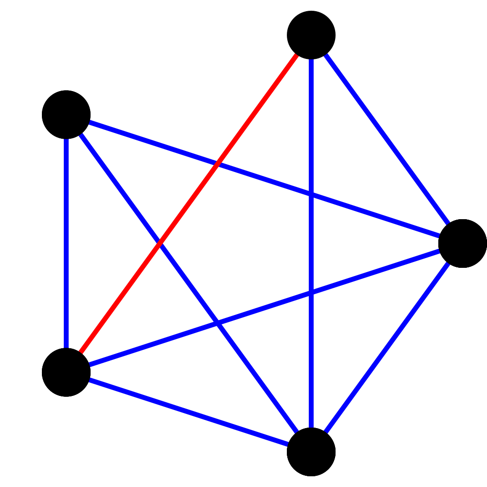
(a) $\mathtt{ffuv0}$

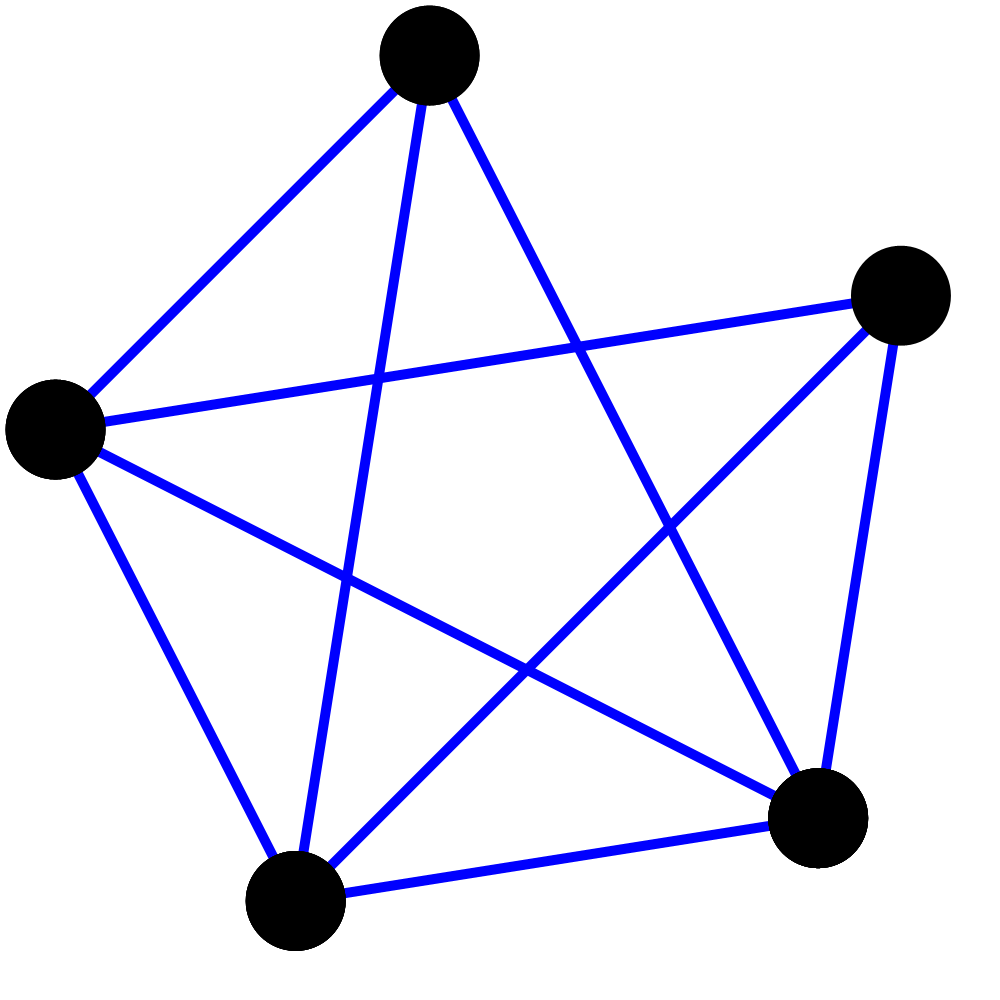
(b) $\mathtt{fguv0}$

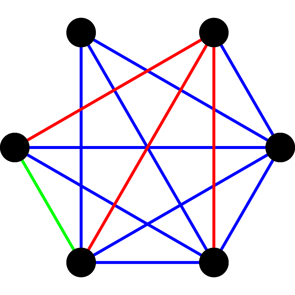
(c) $\mathtt{fguvs}$

Figure 6: 4-colorings of the minimal relaxations used in our implementation of solvers for the $\mathtt{ffuv0}$, $\mathtt{fguv0}$ and $\mathtt{fguvs}$ problems.

10 Enumerating minimal problems —
additional details

Returning to the enumeration problem described in in Section 3, we now discuss line graphs, a standard graph-theoretic construction. The utility of this construction is that the isomorphism class of a $4$-coloring is completely determined by an associated line graph $\mathcal{L}(c)$ after equipping it with a suitable vertex labeling. The vertices of the line graph $\mathcal{L}(c)$ are simply the non-white edges, and an edge between two vertices of $\mathcal{L}(c)$ exists whenever the two non-white edges share a vertex between $1$ and $N$. We label each vertex $pq\in\mathcal{L}(c)$ by its color $c(pq).$ Two isomorphic graphs have isomorphic line graphs; conversely, a classical theorem of Whitney [52] implies that two connected graphs whose line graphs are isomorphic are themselves isomorphic, with the sole exception of the complete graph $K_{3}$ and the claw graph $K_{1,3}$ (see eg. [18, Theorem 8.3].) Although $\mathcal{L}(K_{3})\cong\mathcal{L}(K_{1,3})$, the original graphs $K_{3}$ and $K_{1,3}$ have different numbers of edges. From this, it easily follows that we can decide whether or not two $4$-colorings $c_{1},c_{2}$ are isomorphic: form the two graphs $\mathcal{L}(c_{1})$ and $\mathcal{L}(c_{2})$, decide if there exists an isomorphism that respects their labelings, and repeat this same procedure for the two graphs $\mathcal{L}(c_{1}),\mathcal{L}(c_{2}\circ\tau),$ where $\tau$ swaps green and red edges.

We implement software based on the NetworkX library [35], and the VF2++ algorithm [25] to compute the isomorphism classes for all minimal problems listed in Tab. 1. The code is implemented in Python and is publicly available at github.com/andreadalcin/MinimalPerspectiveAutocalibration.

Tab. 6 provides a visualization of one representative 4-coloring for each isomorphism class for the $\mathtt{fguv0},\mathtt{fgu00},\mathtt{fg000}$ minimal problems in $M=3$ views. The isomorphism classes for $\mathtt{fguvs}$ are too many to be visualized in Tab. 6. Still, as part of our software, we provide a visualization tool and instruction to visualize equivalence classes for $\mathtt{fguvs}$.

Prior on $K$	$M$	$N$	$L$	Sol. in $\mathbb{C}$ for isomorphism class								#$\mathbf{g}$
$\mathtt{fguv0}$	3	5	1	2313	2313	2313						3
$\mathtt{fgu00}$	3	5	2	9686	9686	9686	9686	9686	33606	33606	33606	8
$\mathtt{fg000}$	3	5	3	17624	17624	17624	3884	3884	3884	3884	19696	37
				19696	19696	19696	19696	19696	21696	21696	21696
				21696	21696	16356	28640	16948	29888	74056	76832
				74480	31183	87328	17364	77816	31964	33262	88000
				33884	171696	198032	193648	207664

Table 6: Visualization of Isomorphism Classes. Visualization of one representative 4-coloring for each isomorphism class of minimal relaxations for autocalibration problems $\mathtt{fguv0}$, $\mathtt{fgu00}$, $\mathtt{fg000}$ in $M=3$ views. For each triplet $(\mathtt{fguvs},M,N)$, we report one representative 4-coloring for each isomorphism class and its associated solution count in $\mathbb{C}$. Solution counts refer to unknown depths and the parameters of $\omega$ in (2)–(4).

11 Experiments

We provide additional details on our experimental validation that were omitted from the main paper due to space restrictions.

11.1 Choice of Minimal Relaxations

In case of different minimal relaxations yielding the same minimum solution count, e.g., in $\mathtt{fguv0}$, we selected that yielding the lowest mean reprojection error in our synthetic test described in Sec. 4.1. We noted that reprojection error fluctuations among different relaxations with identical solution counts are always below 1%, suggesting comparable numerical performance between different minimal relaxations with the same solution count.

For the purposes of this work, we list the specific minimal relaxations used to implement the solvers $\mathtt{ffuv0}$, $\mathtt{fguv0}$, and $\mathtt{fguvs}$, which are used throughout our experiments. Specifically, for each implemented solver, we specify the depth constraints that are omitted from the chosen system of equations $\mathbf{g}$:

• $\mathtt{ffuv0}$: $d_{1,2,45}$, $d_{1,3,45}$, $d_{1,2,35}$ (see Fig. 6(a)).

• $\mathtt{fguv0}$: $d_{1,2,45}$, $d_{1,3,45}$ (see Fig. 6(b)).

• $\mathtt{fguvs}$: $d_{1,2,56}$, $d_{1,3,56}$, $d_{1,2,45}$, $d_{1,3,45}$, $d_{1,2,46}$, $d_{1,2,36}$, $d_{1,2,26}$, $d_{1,3,34}$ (see Fig. 6(c)).

Our public code also includes starting the parameters and solutions for parameter homotopies used by each solver to ensure full reproducibility.

11.2 Computing Camera Rotations and Centers from Projective Depths

We discuss the conversion of projective depths into camera rotations and centers. Referring to Sec. 4, our autocalibration formulation allows us to perform an Euclidean reconstruction. However, we obtain the projective depths associated with image points rather than camera roto-translations and 3D point coordinates. However, recovering camera rotations and centers is straightforward, assuming that, without loss of generality, the $i=1$ camera is at $R_{1}=I$ and $C_{1}=0$.

Initially, we compute 3D points, denoted as $X_{ip}$, for each camera $i\in[M]$, using $X_{ip}=\lambda_{ip}K^{-1}x_{ip}$. Throughout this section, we express $X_{ip}$ in Cartesian coordinates, i.e., $X_{ip}\in\mathbb{R}^{3}$. Centering all 3D points by subtracting $X_{11}$ (the point $p=1$ seen by the $i=1$ camera), we extract translation components $t_{i}=X_{i1}$ for $i\in[2,\ldots,M]$. Subtracting the translation component from the 3D points seen by the $i$-th view ($\tilde{X}_{ip}=X_{ip}-t_{i}$), we compute the rotation component

$$R_{i}=\left(\!\!\begin{array}[]{ccc}\tilde{X}_{i2}&\tilde{X}_{i3}&\tilde{X}_{i4}\end{array}\!\!\right)\left(\!\!\begin{array}[]{ccc}\tilde{X}_{12}&\tilde{X}_{13}&\tilde{X}_{14}\end{array}\!\!\right)^{-1}\;.$$ (19)

Finally, we compute the camera centers

$$C_{i}=\lambda_{i2}K^{-1}x_{i2}-R_{i}\lambda_{12}K^{-1}x_{12}\,,\quad i\in[2,\ldots,M]\;.$$ (20)

As discussed in Sec. 6, a given relaxation might remove constraints that enforce the validity of the recovered rotation matrices, i.e., $R_{i}\in\mathrm{SO}(3)$. If $R_{i}$ is not an orthogonal matrix, we compute an SVD $R_{i}=USV^{\top}$ and the closest orthogonal matrix $\tilde{R}_{i}=UV^{\top}$ (with respect to either the Frobenius or spectral norm.)

This approach is consistently applied in our experimental validation, and we provide Julia code for the conversion from projective depth to camera roto-translation.

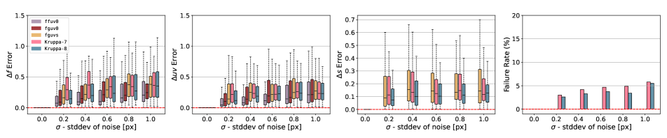
Figure 7: Kruppa-7 Evaluation on Synthetic Images. Solver accuracy is assessed under varying levels of zero-mean Gaussian noise (denoted by $\sigma$ on the x-axis) applied to pixel coordinates. Mean reprojection error and relative errors in focal lengths $\Delta fg$, principal point $\Delta uv$, and skew $\Delta s$ are reported. For error measures, boxes represent the interquartile range of error distribution. The right-most plot illustrates the failure rate as a percentage, with $\mathtt{fguv0}$, $\mathtt{ffuvs}$, and $\mathtt{fguvs}$ excluded due to no failures. Results are averaged for 1000 synthetic image sequences. Synthetic camera parameters are set to mirror the configuration described in Sec. 4.1. Results are averaged over 1000 synthetic image sequences.

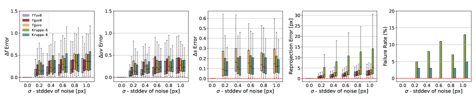
Figure 8: Autocalibration Evaluation on Synthetic Images with Specialized Intrinsics. Solver accuracy is assessed under varying levels of zero-mean Gaussian noise (denoted by $\sigma$ on the x-axis) applied to pixel coordinates. Mean reprojection error and relative errors in focal lengths $\Delta fg$, principal point $\Delta uv$, and skew $\Delta s$ are reported. For error measures, boxes represent the interquartile range of error distribution. The right-most plot illustrates the failure rate as a percentage, with $\mathtt{ffuv0}$, $\mathtt{fguv0}$, and $\mathtt{fguvs}$ excluded due to no failures. Synthetic camera parameters vary across solvers to match their prior camera knowledge. For $\mathtt{fguv0}$ we set $s=0$, and for $\mathtt{ffuv0}$ we set $f=g=330$. Results are averaged over 1000 synthetic image sequences.

	Fountain-P11				Rathaus				KITTI-Depth
Variant	$\Delta fg\downarrow$	$\Delta uv\downarrow$	$Re$	Points3D	$\Delta fg\downarrow$	$\Delta uv\downarrow$	$Re$	Points3D	$\Delta fg\downarrow$	$\Delta uv\downarrow$	$Re$	Points3D
$\text{COLMAP}_{\mathrm{guess}}$	0.3350	0.0140	0.444	4848	0.0671	0.0812	0.624	847	0.6510	0.1360	0.810	210
$\text{COLMAP}_{\texttt{ffuv0}}$	0.0053	0.0281	0.238	5357	0.0215	0.0102	0.441	831	0.0698	0.0161	0.402	231
$\text{COLMAP}_{\texttt{fguv0}}$	0.0058	0.0297	0.241	5356	0.0237	0.0111	0.450	823	0.0720	0.0185	0.409	231
$\text{COLMAP}_{\mathrm{guess}}$ + $K\text{-BA}$	0.0012	0.0013	0.212	5296	0.0185	0.0607	0.435	868	0.3480	0.5072	0.547	232
$\text{COLMAP}_{\texttt{ffuv0}}$ + $K\text{-BA}$	0.0011	0.0012	0.212	5367	0.0165	0.0305	0.431	823	0.0691	0.1281	0.401	236
$\text{COLMAP}_{\texttt{fguv0}}$ + $K\text{-BA}$	0.0011	0.0012	0.212	5367	0.0165	0.0307	0.432	823	0.0626	0.1773	0.404	236
$\text{COLMAP}_{\mathrm{gt}}$ + $K\text{-BA}$	0.0013	0.0011	0.210	5368	0.0069	0.0291	0.430	794	0.0401	0.0553	0.398	237

Table 7: Comparing errors and numbers of registered points for autocalibration strategies in COLMAP.

11.3 Error Metrics

We provide complete error definitions for the error metrics employed in our experimental evaluation within the main paper. Referring to Sec. 4, we define the relative error $\Delta fg$ in focal lengths as follows:

$$\small\Delta fg=\frac{1}{2}\left(\frac{|\hat{f}-f_{\mathrm{gt}}|}{f_{\mathrm{gt}}}+\frac{|\hat{g}-g_{\mathrm{gt}}|}{g_{\mathrm{gt}}}\right).$$ (21)

The reprojection error $Re$ is computed as

$$Re=\frac{1}{N(M-1)}\sum_{i=2}^{M}\sum_{p=1}^{N}\|x_{ip}-\hat{x}_{ip}\|_{2}\;,$$ (22)

where $\hat{x}_{ip}$ denotes the projection of the $p$-th point onto the $i$-th view using the estimated camera parameters:

$$\hat{x}_{ip}=\frac{1}{\hat{\lambda}_{ip}}\hat{K}\,\hat{R}_{i}\left(\!\!\begin{array}[]{c}I\mid-\hat{C}_{i}\end{array}\!\!\right)\left(\!\!\begin{array}[]{c}\hat{\lambda}_{1p}\hat{K}^{-1}x_{1p}\\ 1\end{array}\!\!\right)\;,$$ (23)

where $\hat{K},\hat{R}_{i},\hat{C}_{i},\hat{\lambda}_{ip}$ denote the estimated camera intrinsics, rotation, center, and projective depth of point $p$ seen by view $i$, respectively. The definition of the reprojection error $Re_{\mathrm{gt}}$ is consistent with (22), but $\hat{x}_{ip}$ is computed as:

$$\hat{x}_{ip}=\frac{1}{\hat{\lambda}_{ip}}\hat{K}\,R_{i}\left(\!\!\begin{array}[]{c}I\mid-C_{i}\end{array}\!\!\right)\left(\!\!\begin{array}[]{c}\hat{\lambda}_{1p}\hat{K}^{-1}x_{1p}\\ 1\end{array}\!\!\right)\;,$$ (24)

where $R_{i},C_{i}$ are the ground truth camera rotation and center, respectively.

In Sec. 4.2, the angular errors $\epsilon_{R}$ and $\epsilon_{C}$ for estimated camera rotations and centers, respectively, are defined as follows:

$$\epsilon_{R} =\frac{1}{M-1}\sum_{i=2}^{M}\left|\;\arccos\left(\frac{\textrm{tr}(R_{i}^{\top}\hat{R}_{i})-1}{2}\right)\;\right|\;,$$ (25)

$$\epsilon_{C} =\frac{1}{M-1}\sum_{i=2}^{M}\left|\;\arccos\left(\frac{C_{i}^{\top}\hat{C}_{i}}{\|C_{i}\|\|\hat{C}_{i}\|}\right)\;\right|\;,$$ (26)

where $\hat{R}_{i},\hat{C}_{i}$ denote the estimated rotation and camera center, respectively, of the $i$-th camera with respect to the $i=1$ camera, for which $R_{1}=I$ and $C_{1}=[0,0,0]$. $R_{i},C_{i}$ denote the ground truth camera rotation and center, respectively. The values of $\epsilon_{R}$ and $\epsilon_{C}$ are expressed in degrees for all experiments.

11.4 Synthetic Experiments — additional details

We provide additional details regarding our synthetic evaluation, referring to Sec. 4.1 of the main paper.

Kruppa-7. Fig. 7 presents a comparative analysis of the results achieved by the Kruppa-7 solver in relation to the $\mathtt{ffuv0}$, $\mathtt{fguv0}$, $\mathtt{fguvs}$, and Kruppa-8 solvers. Results reveal that Kruppa-7 exhibits inferior accuracy in focal length estimation ($\Delta fg$) compared to Kruppa-8, especially at lower noise levels $\sigma\geq 0.6$. Nonetheless, principal point and skew estimation accuracy are comparable to Kruppa-8. Finally, the failure rates of Kruppa-7 match or surpass those of Kruppa-8 across all noise levels $\sigma$.

Evaluation with Specialized Intrinsics. Fig. 8 presents the results of our $\mathtt{ffuv0}$ and $\mathtt{fguv0}$ solvers evaluated on synthetic scenes generated using varying camera parameters that depend on the prior camera knowledge assumed by each solver. For $\mathtt{fguvs}$, Kruppa-6, and Kruppa-8, which do not assume any camera knowledge, synthetic camera parameters are set to $f=330$, $g=310$, $u=300$, $v=250$, and $s=10$. For $\mathtt{fguv0}$, which assumes zero-skew, we set $s=0$. Finally, for $\mathtt{ffuv0}$, which assumes squared pixel aspect ratio, we set $f=g=330$.

The results affirm that $\mathtt{ffuv0}$ and $\mathtt{fguv0}$ excel in focal length estimation and achieve comparable performance to the other solvers in principal point estimation. As expected, errors $\Delta fg$ and $\Delta uv$ are reduced due to the synthetic camera parameters perfectly matching the prior knowledge assumed by each of these solvers.

This evaluation also focuses on evaluating the theoretical correctness of our solvers, i.e., verifying that zero error is achieved in the noiseless case. Both $\mathtt{ffuv0}$ and $\mathtt{fguv0}$ attain zero errors when $\delta=0$ and their assumed prior knowledge matches the ground truth camera parameters, confirming their theoretical correctness. As expected, our solvers do not exhibit any failures in this synthetic evaluation.

Degeneracies. As discussed in Sec. 4.1, our proposed autocalibration solvers are unaffected by the degeneracy of Kruppa-based methods arising from a singularity in the Kruppa equations when the optical centers of cameras lie on a sphere, and their optical axes intersect at the sphere’s center [49]. To verify that our solvers overcome this substantial problem, we synthetically reproduce the aforementioned degeneracy condition and assess calibration on these generated image sequences. We generate 1000 synthetic scenes that exhibit the degeneracy condition of Kruppa and verify our $\mathtt{ffuv0}$, $\mathtt{fguv0}$ and $\mathtt{fguvs}$ can successfully perform autocalibration in all cases, exhibiting zero-error in the noiseless case and a failure rate of 0%.

Furthermore, referring to Sec. 3.3, we confirm the well-posed nature of our autocalibration problem by verifying that the Jacobian of the given relaxed system $\mathbf{g}(\mathbf{p},\mathbf{x})=0$ is full-rank at the synthetic solution $(\mathbf{p}_{0},\mathbf{x}_{0})$. Additionally, we observe that the least singular value of the Jacobian of the system never falls below $10^{-4}$ in our testing. This indicates the robust numerical stability of our solvers.

We implement code to generate degenerate image sequences for Kruppa equations and verify that our solvers are unaffected by this problem. The code is implemented in Julia and is publicly available at github.com/andreadalcin/MinimalPerspectiveAutocalibration.

11.5 Autocalibration in COLMAP —
additional details

Finally, we provide further details on evaluating the COLMAP integration of our autocalibration solvers.

Datasets. For Fountain-P11 [47], we consider the 0-2-4 and 0-3-6 image triplets. Rathaus [47] includes a single calibrated image triplet. For KITTI-Depth [16], we extract image triplets from the 2011-09-26-drive-0005 sequence.

Results. Tab. 7 provides an extended view of Tab. 3, including the results achieved by $\text{COLMAP}_{\mathtt{ffuv0}}$ — the initialization strategy of $K$ based on the $\mathtt{ffuv0}$ solver. This variant excludes $K$ from Bundle Adjustment (BA), and we present results achieved by $\text{COLMAP}_{\mathtt{ffuv0}}$ when BA is applied to $K$. The calibration accuracy of $\text{COLMAP}_{\mathtt{ffuv0}}$ surpasses that of $\text{COLMAP}_{\mathtt{fguv0}}$ marginally, particularly in terms of principal point estimation ($\Delta uv$). When Bundle Adjustment is extended to $K$, the disparity in performance diminishes and becomes negligible, especially in the Fountain-P11 and Rathaus datasets. Notably, in KITTI-Depth, extending Bundle Adjustment to $K$ shows that $\text{COLMAP}_{\mathtt{ffuv0}}$ achieves a slightly lower accuracy in focal lengths ($\Delta fg$) but exhibits improved accuracy in the principal point ($\Delta uv$).

Discussion. In the context of integrating our autocalibration solvers into COLMAP, both $\mathtt{ffuv0}$ and $\mathtt{fguv0}$ demonstrate similar accuracy in both $\Delta fg$ and $\Delta uv$, particularly when extending Bundle Adjustment to $K$. Consequently, opting for $\mathtt{fguv0}$ as an initialization strategy in COLMAP is preferable for many practical applications. This preference is attributed to the faster processing speed of $\mathtt{fguv0}$ over $\mathtt{ffuv0}$ (1.78 s/iter compared to 9.21 s/iter) and its support for cameras without square pixel aspect ratio.

References

- [1] Sylvain Bougnoux. From projective to Euclidean space under any practical situation, a criticism of self-calibration. In Proceedings of the Sixth International Conference on Computer Vision (ICCV-98), Bombay, India, January 4-7, 1998, pages 790–798. IEEE Computer Society, 1998.
- [2] Paul Breiding and Sascha Timme. HomotopyContinuation.jl: A Package for Homotopy Continuation in Julia. In International Congress on Mathematical Software, pages 458–465. Springer, 2018.
- [3] Martin Bråtelund and Felix Rydell. Compatibility of fundamental matrices for complete viewing graphs. In Proceedings of the IEEE/CVF International Conference on Computer Vision (ICCV), pages 3328–3336, October 2023.
- [4] Manmohan Krishna Chandraker, Sameer Agarwal, David J. Kriegman, and Serge J. Belongie. Globally optimal affine and metric upgrades in stratified autocalibration. In IEEE 11th International Conference on Computer Vision, ICCV 2007, Rio de Janeiro, Brazil, October 14-20, 2007, pages 1–8. IEEE Computer Society, 2007.
- [5] Manmohan Krishna Chandraker, Sameer Agarwal, David J. Kriegman, and Serge J. Belongie. Globally optimal algorithms for stratified autocalibration. Int. J. Comput. Vis., 90(2):236–254, 2010.
- [6] David A. Cox, John Little, and Donal O’Shea. Ideals, varieties, and algorithms. Undergraduate Texts in Mathematics. Springer, 4 ed. edition, 2015.
- [7] Timothy Duff, Cvetelina Hill, Anders Jensen, Kisun Lee, Anton Leykin, and Jeff Sommars. Solving polynomial systems via homotopy continuation and monodromy. IMA Journal of Numerical Analysis, 2018.
- [8] Timothy Duff, Kathlén Kohn, Anton Leykin, and Tomas Pajdla. PLMP - Point-line Minimal Problems in Complete Multi-view Visibility. In 2019 IEEE/CVF International Conference on Computer Vision, ICCV 2019, Seoul, Korea (South), October 27 - November 2, 2019, pages 1675–1684. IEEE, 2019.
- [9] Timothy Duff, Kathlén Kohn, Anton Leykin, and Tomas Pajdla. PLP - point-line minimal problems under partial visibility in three views. In Andrea Vedaldi, Horst Bischof, Thomas Brox, and Jan-Michael Frahm, editors, Computer Vision - ECCV 2020 - 16th European Conference, Glasgow, UK, August 23-28, 2020, Proceedings, Part XXVI, volume 12371 of Lecture Notes in Computer Science, pages 175–192. Springer, 2020.
- [10] Timothy Duff, Viktor Korotynskiy, Tomas Pajdla, and Margaret H. Regan. Galois/monodromy groups for decomposing minimal problems in 3D reconstruction. SIAM Journal on Applied Algebra and Geometry, 2022.
- [11] Olivier D. Faugeras, Quang-Tuan Luong, and Stephen J. Maybank. Camera self-calibration: Theory and experiments. In Giulio Sandini, editor, Computer Vision - ECCV’92, Second European Conference on Computer Vision, Santa Margherita Ligure, Italy, May 19-22, 1992, Proceedings, volume 588 of Lecture Notes in Computer Science, pages 321–334. Springer, 1992.
- [12] Andrea Fusiello. Uncalibrated Euclidean reconstruction: a review. Image and Vision Computing, 18(6-7):555–563, 2000.
- [13] Andrea Fusiello, Arrigo Benedetti, Michela Farenzena, and Alessandro Busti. Globally convergent autocalibration using interval analysis. IEEE Trans. Pattern Anal. Mach. Intell., 26(12):1633–1638, 2004.
- [14] Guillermo Gallego, Elias Mueggler, and Peter F. Sturm. Translation of “Zur Ermittlung eines Objektes aus zwei Perspektiven mit innerer Orientierung” by Erwin Kruppa (1913). CoRR, abs/1801.01454, 2018.
- [15] Amnon Geifman, Yoni Kasten, Meirav Galun, and Ronen Basri. Averaging essential and fundamental matrices in collinear camera settings. In 2020 IEEE/CVF Conference on Computer Vision and Pattern Recognition, CVPR 2020, Seattle, WA, USA, June 13-19, 2020, pages 6020–6029. Computer Vision Foundation / IEEE, 2020.
- [16] Andreas Geiger, Philip Lenz, and Raquel Urtasun. Are we ready for autonomous driving? the KITTI vision benchmark suite. In 2012 IEEE conference on computer vision and pattern recognition, pages 3354–3361. IEEE, 2012.
- [17] Riccardo Gherardi and Andrea Fusiello. Practical autocalibration. In Computer Vision–ECCV 2010: 11th European Conference on Computer Vision, Heraklion, Crete, Greece, September 5-11, 2010, Proceedings, Part I 11, pages 790–801. Springer, 2010.
- [18] Frank Harary. Graph theory. Addison-Wesley Publishing Co., Reading, Mass.-Menlo Park, Calif.-London, 1969.
- [19] R.I. Hartley. Kruppa’s equations derived from the fundamental matrix. IEEE Transactions on Pattern Analysis and Machine Intelligence, 19(2):133–135, 1997.
- [20] R. Hartley and A. Zisserman. Multiple view geometry in Computer Vision. Cambridge University Press, Cambridge, second edition, 2003. With a foreword by Olivier Faugeras.
- [21] Richard I Hartley. Euclidean reconstruction from uncalibrated views. In Joint European-US workshop on applications of invariance in computer vision, pages 235–256. Springer, 1993.
- [22] Richard I. Hartley. In Defence of the 8-Point Algorithm. In Procedings of the Fifth International Conference on Computer Vision (ICCV 95), Massachusetts Institute of Technology, Cambridge, Massachusetts, USA, June 20-23, 1995, pages 1064–1070. IEEE Computer Society, 1995.
- [23] Anders Heyden and Kalle Åström. Flexible calibration: Minimal cases for auto-calibration. In Proceedings of the International Conference on Computer Vision, Kerkyra, Corfu, Greece, September 20-25, 1999, pages 350–355. IEEE Computer Society, 1999.
- [24] Petr Hruby, Timothy Duff, Anton Leykin, and Tomás Pajdla. Learning to solve hard minimal problems. In IEEE/CVF Conference on Computer Vision and Pattern Recognition, CVPR 2022, New Orleans, LA, USA, June 18-24, 2022, pages 5522–5532. IEEE, 2022.
- [25] Alpár Jüttner and Péter Madarasi. Vf2++—an improved subgraph isomorphism algorithm. Discrete Applied Mathematics, 242:69–81, 2018.
- [26] Yoni Kasten, Amnon Geifman, Meirav Galun, and Ronen Basri. Algebraic characterization of essential matrices and their averaging in multiview settings. In 2019 IEEE/CVF International Conference on Computer Vision, ICCV 2019, Seoul, Korea (South), October 27 - November 2, 2019, pages 5894–5902. IEEE, 2019.
- [27] Joe Kileel. Minimal problems for the calibrated trifocal variety. SIAM Journal on Applied Algebra and Geometry, 1(1):575–598, 2017.
- [28] Erwin Kruppa. Zur Ermittlung eines Objektes aus zwei Perspektiven mit innerer Orientierung. Hölder, 1913.
- [29] David G Lowe. Distinctive image features from scale-invariant keypoints. International journal of computer vision, 60:91–110, 2004.
- [30] Quang-Tuan Luong and Olivier D. Faugeras. Self-calibration of a moving camera from point correspondences and fundamental matrices. Int. J. Comput. Vis., 22(3):261–289, 1997.
- [31] Quang-Tuan Luong, Rachid Deriche, Olivier Faugeras, and Theodore Papadopoulo. On determining the fundamental matrix: Analysis of different methods and experimental results. PhD thesis, Inria, 1993.
- [32] Yi Ma, René Vidal, Jana Kosecka, and Shankar Sastry. Kruppa equation revisited: Its renormalization and degeneracy. In David Vernon, editor, Computer Vision - ECCV 2000, 6th European Conference on Computer Vision, Dublin, Ireland, June 26 - July 1, 2000, Proceedings, Part II, volume 1843 of Lecture Notes in Computer Science, pages 561–577. Springer, 2000.
- [33] Evgeniy V. Martyushev. A minimal six-point auto-calibration algorithm. http://arxiv.org/abs/1307.3759, 2013.
- [34] Stephen J. Maybank and Olivier D. Faugeras. A theory of self-calibration of a moving camera. Int. J. Comput. Vis., 8(2):123–151, 1992.
- [35] NetworkX Developers. NetworkX, 2023. Accessed: November 24, 2023.
- [36] Danda Pani Paudel and Luc Van Gool. Sampling algebraic varieties for robust camera autocalibration. In Proceedings of the European Conference on Computer Vision (ECCV), pages 265–281, 2018.
- [37] Marc Pollefeys, Luc Van Gool, and André Oosterlinck. The modulus constraint: a new constraint self-calibration. In 13th International Conference on Pattern Recognition, ICPR 1996, Vienna, Austria, 25-19 August, 1996, pages 349–353. IEEE Computer Society, 1996.
- [38] Marc Pollefeys, Reinhard Koch, and Luc Van Gool. Self-calibration and metric reconstruction inspite of varying and unknown intrinsic camera parameters. Int. J. Comput. Vis., 32(1):7–25, 1999.
- [39] Marc Pollefeys and Luc Van Gool. A stratified approach to metric self-calibration. In Proceedings of IEEE computer society conference on computer vision and pattern recognition, pages 407–412. IEEE, 1997.
- [40] Long Quan, Bill Triggs, and Bernard Mourrain. Some results on minimal Euclidean reconstruction from four points. Journal of Mathematical Imaging and Vision, 24:341–348, 2006.
- [41] Torsten Sattler, Chris Sweeney, and Marc Pollefeys. On sampling focal length values to solve the absolute pose problem. In David J. Fleet, Tomas Pajdla, Bernt Schiele, and Tinne Tuytelaars, editors, Computer Vision - ECCV 2014 - 13th European Conference, Zurich, Switzerland, September 6-12, 2014, Proceedings, Part IV, volume 8692 of Lecture Notes in Computer Science, pages 828–843. Springer, 2014.
- [42] Frederik Schaffalitzky, Andrew Zisserman, Richard I Hartley, and Philip HS Torr. A six point solution for structure and motion. In Computer Vision-ECCV 2000: 6th European Conference on Computer Vision Dublin, Ireland, June 26–July 1, 2000 Proceedings, Part I 6, pages 632–648. Springer, 2000.
- [43] Johannes Lutz Schönberger and Jan-Michael Frahm. Structure-from-motion revisited. In Conference on Computer Vision and Pattern Recognition (CVPR), 2016.
- [44] Johannes Lutz Schönberger, Enliang Zheng, Marc Pollefeys, and Jan-Michael Frahm. Pixelwise view selection for unstructured multi-view stereo. In European Conference on Computer Vision (ECCV), 2016.
- [45] Andrew J. Sommese and Charles W. Wampler, II. The numerical solution of systems of polynomials arising in engineering and science. World Scientific, Hackensack, NJ, 2005.
- [46] Henrik Stewénius, David Nistér, Fredrik Kahl, and Frederik Schaffalitzky. A minimal solution for relative pose with unknown focal length. Image and Vision Computing, 26(7):871–877, 2008.
- [47] Christoph Strecha, Wolfgang Von Hansen, Luc Van Gool, Pascal Fua, and Ulrich Thoennessen. On benchmarking camera calibration and multi-view stereo for high resolution imagery. In 2008 IEEE conference on computer vision and pattern recognition, pages 1–8. Ieee, 2008.
- [48] Peter Sturm. Critical motion sequences for monocular self-calibration and uncalibrated Euclidean reconstruction. In Proceedings of IEEE Computer Society Conference on Computer Vision and Pattern Recognition, pages 1100–1105. IEEE, 1997.
- [49] P. Sturm. A case against Kruppa’s equations for camera self-calibration. IEEE Transactions on Pattern Analysis and Machine Intelligence, 22(10):1199–1204, 2000.
- [50] Philip HS Torr and Andrew Zisserman. MLESAC: A new robust estimator with application to estimating image geometry. Computer vision and image understanding, 78(1):138–156, 2000.
- [51] Bill Triggs. Autocalibration and the absolute quadric. In 1997 Conference on Computer Vision and Pattern Recognition (CVPR ’97), June 17-19, 1997, San Juan, Puerto Rico, pages 609–614. IEEE Computer Society, 1997.
- [52] Hassler Whitney. Congruent graphs and the connectivity of graphs. Hassler Whitney Collected Papers, pages 61–79, 1992.
- [53] Cyril Zeller and Olivier Faugeras. Camera self-calibration from video sequences: the Kruppa equations revisited. PhD thesis, INRIA, 1996.