Periodic Solutions in a Simple Delay Differential Equation
Abstract
Simple form scalar differential equation with delay and nonlinear negative periodic feedback is considered. The existence of several types of slowly oscillating periodic solutions is shown with the same and double periods of the feedback coefficient. The periodic solutions are built explicitly in the case of piecewise constant nonlinearities involved. The periodic dynamics are shown to persist under small perturbations of the equation which make it smooth. The theoretical results are verified by extensive numerical simulations.
keywords:
delay differential equations; periodic negative feedback; slowly oscillating solutions; periodic solutions; piecewise constant nonlinearities; explicit piecewise affine solutions; reduction to interval maps[inst1]organization=Department of Mathematics,addressline=Pennsylvania State University, country=USA
[inst2]organization=College of Science and Engineering,addressline=Flinders University, country=Australia
1 Introduction
The simple form delay differential equation (DDE)
| (1) |
represents a broad variety of complex dynamical behaviors that can happen in delay differential models. It is also one of the most studied equations in the field exhibiting the range of diverse dynamics from global stability of equilibria to instability and existence of periodic solutions and chaotic behaviours (in contrast to analogous ordinary differential equations). Basic and fundamental facts about the DDE (1) can be found in many sources, see e.g. monographs [2, 3, 10, 19], among others.
Equation (1) is also extensively used as a mathematical model of a variety of real world phenomena, most notably in biological applications; see e.g. the monographs [2, 6, 14, 19] and further references therein. Among the well known and most studied models of type (1) are the Mackey-Glass physiological equations [6, 16], Wazewska-Lasota blood cell model [21], Nicholson’s blowfly equations [7, 17], and several others [2, 14, 19].
Some of the more accurate and adequate mathematical models are explicitly time-dependent, which take into account certain intrinsic periodicity factors, such as e.g. circadian rhythms and seasonal changes. Examples of such differential delay models can be found in publications [1, 5, 6, 14, 15, 22]. Therefore, a natural generalization of equation (1) is the following DDE
| (2) |
where and are -periodic functions, and the nonlinearity satisfies appropriate feedback conditions. An important theoretical and applied question then arises whether the DDE (2) admits periodic solutions, which are induced by the periodicity in the coefficients and . Therefore, the mathematical problem to address is to derive conditions under which equation (2) possesses a nontrivial -periodic solution. This research work is our initial attempt to answer this question for some specific partial cases of the equation under consideration.
This paper deals with the problem of existence of periodic solutions for the simplest possible scalar differential delay equation of the type (2) when ,
| (3) |
and where is a continuous function satisfying the negative feedback assumption the coefficient is a continuous periodic function with the period satisfying and is a delay. The principal problem we are addressing in this work is to derive conditions on the parameters and nonlinearities of equation (3) which would yield the existence of periodic solutions with the same period as the coefficient Though there are some results on the existence of periodic solutions for the DDEs with periodic coefficients none of them is applicable to the simplest form equation (3), to the best of our assessment and knowledge. In many cases that are published in the research literature the generalization from the autonomous case to the period one leads to the loss of the steady positive equilibrium. In some others the equilibrium state persists, however, the sufficient conditions for the existence of periodic solutions cannot distinguish between the nontrivial periodic solutions and the steady state. See more details on such relevant results and further references in e.g. [1, 4, 5, 15, 22].
We are stating and dealing with the problem of existence of nontrivial periodic solutions in the simple form DDE (3). Due to the negative feedback assumption on this equation always admits the trivial constant solution . The mathematical problem is to find periodic solutions which are distinct from the trivial one. This is a difficult problem which is largely not addressed on the general theoretical level. One way to pave a path for a systematic analysis in this direction is to consider model equations of the form given by equation (3) with simple and .
We first construct the periodic solutions in an explicit form by using piecewise constant functions (both the nonlinearity and the coefficient ). Then we modify both functions to be continuous and “close” to the piecewise constant ones, by “smoothing” them in a small neighborhood of the discontinuity set (they can also be made of the type). The periodic dynamics and their stability are shown to persist under such small perturbations.
The paper is structured as follows. First section “Preliminaries” contains basics of the DDE (3) and preliminary results from our recent conference papers [11, 12] necessary for the exposition in subsequent sections. Section 3 deals with periodic solutions of equation (3) explicitly constructed for the initially piecewise constant nonlinearity and the coefficient . The dynamics on a set of slowly oscillating solutions are reduced to that for induced one-dimensional maps, thus proving both the existence of periodic solutions and the types of their stability. In Section 3 it is shown that the dynamics of the interval maps and the periodic solutions from section 2 persist when the defining functions and of equation (3) are replaced by close to them continuous or smoothed functions. The arguments of small regular perturbations of dynamics by DDE (3) are used, which are behind such “small modifications”. The theoretical derivations and exact analytical calculations are verified by extensive numerical simulations.
2 Preliminaries
We focus in this work on the particular case and when equation (1) becomes
| (4) |
Note that the case of general delay is easily reduced to the standard consideration by the time scaling .
Given an initial function in the standard phase space the corresponding solution to equation (4) is easily found for all by consecutive forward integration (the step method). Let be the shift in by time along the solutions of delay differential equation (4), that is . It is a straightforward observation that a fixed point of the shift by period , , gives rise to a periodic solution of the DDE (4). Under such an interpretation, the zero solution is a result of the trivial fixed point , which always exists for DDE (4), due to the negative feedback assumption. The mathematical problem is to derive conditions for the existence of non-trivial fixed points of the shift operator , which is a principal objective of this work.
A solution is called oscillating if it has an infinite sequence of zeros , and is not an identical zero eventually (on any interval of the form )). An oscillating solution is called slowly oscillating, if the sequence of zeros is such that the distance between consecutive zeros is greater than the delay, i.e.
Sufficient conditions for the oscillation of all solutions to equation (4) are well known, see e.g. [8] and further references therein. With the negative feedback assumption and the non-negativity of the coefficient they are that either is sufficiently large, and the coefficient is separated from zero, , or and is large enough (in both cases the product must be sufficiently large). These conditions are satisfied for our considerations to follow in next sections, where the functions and are smoothed continuous ones derived from the initial piecewise constant functions (the piecewise constant case can be viewed as a limit of the continuous one).
We deal in this paper with the slowly oscillating solutions to equation (4). The slowly oscillating solutions are obtained when the initial functions belong to one of the two sign definite cones. Introduce the following two standard subsets of initial functions
Assuming that all solutions to equation (4) oscillate, it is a straightforward calculation to verify that for arbitrary the corresponding solution has an increasing sequence of zeros such that and
| (5) |
In the case when the above inequalities on the consecutive intervals and are reversed into opposite. Therefore, the solution is slowly oscillating. The consecutive intervals , are called semicycles.
Based on the well-known facts [8] and the reasoning above we have the following statement.
Proposition 1
Suppose that the nonlinearity satisfies the negative feedback assumption and . Let the coefficient be - periodic and such that . Assume that . Then for every initial function with the corresponding solution is slowly oscillating with the sequence of simple zeros satisfying the inequalities (5) on the consecutive semicycles. Likewise, for every initial function with the corresponding solution is slowly oscillating satisfying the inequalities opposite to those in (5).
3 Periodic Solutions
In this section the periodic solutions of interest are explicitly constructed based on model piecewise constant nonlinearity and the periodic coefficient . Let and define as follows
| (6) |
Let an initial function be such that either or and . Clearly, the corresponding solution depends on the value only, and does not depend of the particular values of for . In addition, it is uniquely determined by the parameters of the function . The solution is slowly oscillating and piecewise linear (affine) for .
Like in the case of continuous and the corresponding solutions to the DDE (4) with and are slowly oscillating with the consecutive zeros satisfying the inequalities (5). In this case we do not need any additional assumptions on or as in Proposition 1, as the lower rates of growth or decay of any such solution are bounded away from zero (the rates of growth/decay are also bounded from above, due to the boundedness of and ). However, since the constructed solutions are slowly oscillating, we assume that necessarily the assumption must be in place.
In this section we follow and expand on ideas and explicit constructions from our recent work [11, 12]. In particular, functions and are of the same form as in the above papers.
3.1 Periodic solutions with coefficient’s period (Type I)
In this subsection we explicitly construct piecewise affine periodic solutions to equation (4) which are of the same period as the periodic coefficient is. Some of the exposition elements are close and based on results in our recent conference paper [12].
We presume that the desired periodic solutions have the shape as shown in Figure 1. That is, the initial value is determined by an initial function . The corresponding solution has exactly two zeros on the initial period with , for particular assumptions on the parameters . Such assumptions are verified to be valid by the analytical calculations that follow, as well as they are confirmed by corresponding numerical simulations.

It is straightforward to find desired values of the solution for any . We have the following calculations:
where the coefficients of the affine function are given by
| (7) |
It is elementary to deduce that the range for the slope is the open interval with when holds, and when is valid.
A fixed point of the map gives rise to a slowly oscillating periodic solution of equation (4). Moreover, by the affine type of and the construction, such periodic solution is asymptotically stable if , which is equivalent to . The periodic solution is unstable when , which is equivalent to . The unique fixed point is easily found as
| (8) |
Therefore, we arrive at the following statement.
Theorem 1
Let the parameters be given with the values and defined by (7). Then
-
(a)
In case when and are valid, the DDE (4) has an asymptotically stable slowly oscillating -periodic solution.
-
(b)
In the complimentary case when and are valid the equation has an unstable slowly oscillating -periodic solution.
The periodic solutions are generated by the initial function where is given by (8).
Remark 1
-
(a)
The local stability case is equivalent to the relationship . At the same time, in order for the fixed point to be negative, one must assume that . The inequality is valid by the construction. For arbitrary fixed there exists such that the inequalities and are satisfied for all Thus, the required assumptions are met for all sufficiently large This case is treated in more detail in our recent paper [12].
-
(b)
The instability case is equivalent to (note that the case is not possible for any choices of positive and ). In order to have the fixed point negative, one must assume that is satisfied, that is . Since the assumption would imply that . Therefore, given fixed values of there exists such that for all Thus, the required assumptions are met for all sufficiently large
-
(c)
It is clear that due to the continuous dependence of and on the parameters the stable or unstable periodic solutions of Theorem 1 exist on an open box in , each side of which is a corresponding open interval about a specific value of each of the four parameters corresponding to a fixed point . Those boxes can be multiple, as our numerical insight indicates, and they do not overlap for the stable and unstable solutions due to the respective opposite relationship between and .
| 1 | 0.25 | 2.5 | 1.5 | -0.25 | 4 |
| 2 | 0.5 | 2.5 | 2 | -1/3 | 4.5 |
| 2 | 0.25 | 2.5 | 1 | -4/7 | 3.5 |
| 1 | 0.5 | 3 | 1 | -0.5 | 4 |
| 2 | 1 | 3 | 1.5 | -0.5 | 4.5 |
| 2.5 | 0.5 | 3 | 4 | -0.31 | 7 |
| 3 | 0.5 | 3 | 4.5 | -0.45 | 7.5 |
| 4 | 1 | 3.5 | 2 | -2 | 5.5 |
| 5 | 0.5 | 3 | 3 | -1.94 | 6 |
| 5 | 1 | 3 | 2 | -1.88 | 5 |
| -1.0602 |
The parametric range for which Theorem 1 guarantees the existence of slowly oscillating periodic solutions, either stable or unstable, is large.
Note that due to the symmetry property of the nonlinearity (oddness) and the procedure of construction of the periodic solutions , under the assumption of Theorem 1 there also exists the symmetric to periodic solution generated by the initial function . The two periodic solutions are related by , thus, they are symmetric to each other.
A large sample of parametric values has been derived for which numerical periodic solutions have been obtained and confirmed to be of the described form. Table 1 is a sample selection of parametric values resulting in asymptotically stable slowly oscillating periodic solutions given by Theorem 1. The values for these periodic solutions are easily found from the explicit formula (8). They are also verified to exist numerically.
The next Table 2 is a sample selection of unstable slowly oscillating periodic solutions implied by Theorem 1. The values for these periodic solutions are found from formula (8) as well. The unstable periodic solutions cannot be verified numerically as respective initial functions actually generate approximate close nearby solutions (not the exact ones). Those solutions, when calculated in forward time, are repelled for large times by the actual unstable ones and are attracted by stable periodic solutions of double period . The latter are studied analytically and numerically and described in detail in the next subsection.
| 0.5 | 5 | 5 | 1 | -1.31 | 6 |
| 1 | 5 | 4 | 1 | -1.625 | 5 |
| 1 | 7 | 4 | 1 | -1.5 | 5 |
| 1 | 7 | 3 | 2 | -1.0833 | 5 |
| 1.5 | 7 | 2.5 | 2.5 | -1.3295 | 5 |
| 1.5 | 7 | 3.5 | 1.5 | -2.0795 | 5 |
| 1.5 | 7 | 4 | 3 | -4.3636 | 7 |
| 2 | 7 | 3 | 2 | -2.4 | 5 |
| 2 | 7 | 3 | 3 | -4.6 | 6 |
| 2 | 7 | 3.5 | 2.5 | -4.3 | 6 |
| 2.5 | 7 | 2.5 | 2.5 | -1.2614 | 5 |
| 2.5 | 7 | 3 | 2 | -1.5682 | 5 |
| -1.382 |
3.2 Periodic solutions with double coefficient’s period (Type II)
In this subsection we explicitly construct piecewise affine periodic solutions to equation (4) which are of double period of the -periodic coefficient . Some of the exposition is close and based on the results of our recent conference paper [11].
We presume that the desired periodic solutions have the initial shape as shown in Figure 2. That is, the initial value is determined by an initial function . The corresponding solution has exactly one zero on the initial periodic interval with and and . Such assumptions are verified to be valid by the analytical calculations that follow, as well as are confirmed by associated numerical simulations.

It is straightforward to calculate the desired values of as follows:
where
| (9) |
are uniquely defined by the parameters .
Likewise, when and analogous calculations yield
with the same and as in the expression for given by formula (9). It is easy to see that for arbitrary positive the respective values of can only belong to the range with if and if
We are interested in parametric values and initial values such that and . This will be the case when , at least in some vicinity of the discontinuity point . The through map is given by . Its only fixed point is found as , and it is negative when and The fixed point generates an asymptotically stable periodic solution of period , when the initial function for equation (4) is chosen as The periodic solution can also be described in terms of a cycle of period of an appropriate one-dimensional map defined by the maps and introduced above. Namely, define the piecewise affine map for as follows:
The map is discontinuous at and is symmetric (odd) with respect to , . Assuming one can see that the negative feedback condition is satisfied at least locally in a vicinity of . The global dynamics of map is very simple in this case, as described by the following statement:
Proposition 2
Suppose that . Then
-
(i)
If is satisfied, the map has a unique globally attracting cycle of period , given by , where . The -cycle attracts all the initial values in the case when holds, and all the initial values from the interval in the case when holds;
-
(ii)
If is satisfied, the map has no cycles of period 2; moreover, any iterative sequence diverges, .
Therefore, by translating the properties of the interval map to the slowly oscillating solutions of DDE (4), we have the following statement
Theorem 2
Let the parameters be given with values and defined by (9) and . Then, in case when is valid DDE (4) has an asymptotically stable slowly oscillating -periodic solution. The periodic solution is generated by the initial function where . In the case when is valid the equation does not have any -periodic slowly oscillating solutions.
Table 3 provides sample selections of parametric values for which the stable -periodic solutions exist. Besides using formula (8) to calculate respective , their existence was also confirmed numerically.
| 4 | 1 | 0.5 | 2.5 | -0.33 | 6 |
| 4 | 1 | 1 | 3.5 | -0.33 | 9 |
| 5 | 1 | 1 | 3.5 | -0.938 | 9 |
| 5 | 1 | 0.5 | 3 | -0.313 | 7 |
| 6 | 1 | 1 | 3.5 | -1.5 | 9 |
| 6 | 1 | 1 | 4.5 | -0.9 | 11 |
| 6 | 1.5 | 1.0 | 3.5 | -0.5 | 9 |
| 7 | 1.5 | 1.5 | 3.5 | -2.39 | 10 |
| 7 | 2.5 | 2.5 | 2.5 | -2.92 | 10 |
| 7 | 2.5 | 2 | 3 | -1.17 | 10 |
| -1.12 |
3.3 Coexistence of periodic solutions
Any slowly oscillating solution considered above in subsections 3.1 and 3.2 is uniquely defined by the sign definite initial function/values such that , and and by the parameters of the periodic coefficient (note that is fixed). One solves the initial value problem for :
| (10) |
Its solution is easily found to exist for all ; it is uniquely determined by the set of the parameters and the initial value of at .
Instead of the initial time value as in the case above, one can consider a similar initial value problem for any . In particular, in the case of the initial time one is solving the following initial value problem for :
| (11) |
Similarly, its solution is uniquely defined by the set of the parameters and by the initial value at .
Now, due to the -periodicity of the coefficient , one can easily see that the solutions of the two initial value problems (10) and (11) are closely related, with an interchange in the set of the parameters and a time shift. Namely, they are just a time shift by with the parameter interchange in the following sense:
| (12) |
with an appropriate This simple observation allows to conclude the simultaneous existence of periodic solutions of both types I and II, which are described in Theorems 1 and 2. Since the value of the ratio with respect to determines the stability of those periodic solutions, their stability types must be opposite to each other. We have the following statement
Theorem 3
There is an open set of parameters such that the DDE (4) has simultaneously an unstable slowly oscillating -periodic solution of type I and an asymptotically stable -periodic solution of type II. Such two periodic solutions can be paired in the following sense: small perturbations of the unstable solution are repelled by it and attracted by a respective stable solution, as
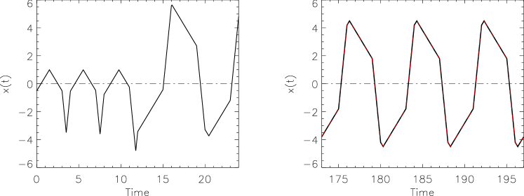
Such situation of coexisting two periodic solutions is depicted in Figure 3. The unstable periodic solution of period is given by Theorem 1 when ; the respective value of is . The stable periodic solution of period is given by Theorem 2 for the parameter values , so that the respective values of and are interchanged for these two solutions. In addition, the solution is shifted by to the right (the graph (b) in Figure 3 shows the solution for longer time intervals).
Tables 4 and 5 provide a sample selection of such dual cases of the coexistence of two types of stable/unstable solutions. Table 5 is a mirror image of Table 4 for the stable periodic solutions with double periods. Namely, each row in Table 5 represents a stable periodic solution of the corresponding unstable solution in the same row number from Table 4.
| 0.5 | 2.5 | 3 | 0.5 | -0.09 | 3.5 |
| 0.5 | 3 | 5 | 1 | -1.35 | 6 |
| 0.5 | 5 | 4 | 0.5 | -0.64 | 4.5 |
| 0.5 | 7 | 3 | 2 | -0.52 | 5 |
| 1 | 6 | 3 | 1 | -0.5 | 4 |
| 1 | 7 | 5 | 1 | -2.67 | 6 |
| 2 | 7 | 2 | 3 | -1.4 | 5 |
| 3 | 7 | 4 | 1 | -5.62 | 5 |
| 1/2 | -0.18 |
| 2.5 | 0.5 | 0.5 | 3 | -0.156 | 7 |
| 3 | 0.5 | 1 | 5 | -0.3 | 12 |
| 5 | 0.5 | 0.5 | 4 | -0.56 | 9 |
| 7 | 0.5 | 2 | 3 | -6.19 | 10 |
| 6 | 1 | 1 | 3 | -1.8 | 8 |
| 7 | 1 | 1 | 5 | -1.17 | 12 |
| 7 | 2 | 3 | 2 | -6.3 | 10 |
| 7 | 3 | 1 | 4 | -4.375 | 10 |
| 1/2 | -1.92 |
4 Smoothed nonlinearities
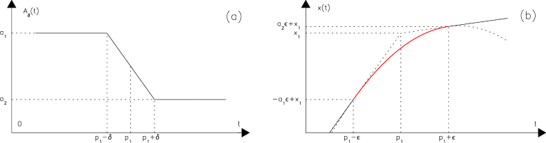
In this section, we follow a standard procedure of replacing the discontinuous piecewise constant functions and by close to them continuous functions and for small . This procedure has been used in numerous cases; typical examples can be found in papers [9, 13, 18, 20]. In a -neighborhood of every discontinuity point for both and the jump discontinuity is replaced by an affine function by connecting the two constant levels by a line segment. That is, define and as follows
| (13) |
and
| (14) |
We shall show next that the values of the piecewise affine slowly oscillating solutions constructed in Section 3 for do not change on the entire periodic interval , except in a small -vicinity of the corner points ( is a multiple of ).
Indeed, the case of a symmetric corner solution, as it passes through a -neighborhood of for the nonlinearity , is shown in Figure 4 (which corresponds to e.g. the Type I solution on the first positive semi-cycle depicted in Figure 1). The -neighborhood of for corresponds to the neighborhood for at . It is immediately clear that the replacement of the corner type solution on the interval by the respective parabolic segment, as a result of the corresponding integration now with a linear nonlinearity , results in a symmetric parabola with the vertex at and the same equal values and as for the initial piecewise solution with the discontinuous .
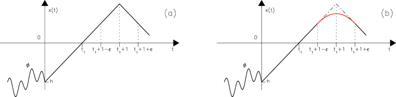
The general case of a corner type solution (piecewise affine) is shown in Figure 5, which corresponds to e.g. point on the graph of a solution of type II (see Figure 2). We shall show now that a smooth parabolic segment solution connecting points and is the precise replacement of the corresponding piecewise affine segment solution which is obtained for the piecewise constant functions and . The values of the solution and its derivatives for the piecewise affine solution are given as
Looking for a parabolic connection as a solution of the DDE (4) on the interval , starting at the point and satisfying the necessary initial-boundary conditions:
one easily finds that the values of the parameters and are:
But then, by checking the value of the parabolic segment of the solution at , one verifies that
which is the same value as the piecewise affine solution at that point.
Thus, the solutions to equation (4) with continuous and , are obtained from the solutions when and by simple cutting out and replacement of the small corner segments by respective parabolic segments, in their -vicinity (). An immediate consequence of this fact is that the periodic solutions and their stability persist under such small -perturbations of and in DDE (4).
Indeed, the easiest way to see this is to consider the new starting point for with . Then the corresponding shift map by the period is dynamically equivalent (conjugate) to the respective map constructed in the case of and . But the latter is equivalent to a composition of respective maps derived in Section 3. If one would like to stay with the initial value in the case of continuous then a small adjustment in the considerations should be made. Namely, the new should be introduced, where is the difference between the two solutions of the differential delay equation (4) in the two cases when and small . Such difference is shown in the graph in Figure 4, part (b) and in the graph in Figure 5, part (b) (in both graphs it is positive). In general, such a difference is independent of the value (or equivalent values in other analogous corner situations). Therefore, all the resulting maps derived in Section 3 will become finite compositions of the affine maps of the form where and is one of the elementary maps considered in Subsections 3.1 and 3.2. Therefore, we are in a position to state the following
Theorem 4
Suppose that the parametric values are such that the assumptions of either one of Theorems 1 or 2 are satisfied. Then there exists such that for every the delay differential equation (4) with functions and has a -smooth periodic solution with the same type of stability as in the respective Theorems 1 or 2. Such a solution converges in uniform metric as to the respective periodic solution with the corner type discontinuity for (when ).
Note that the smoothing of both functions and in a -neighborhood of their discontinuity set can be made such that the resulting continuous nonlinearities and are continuously differentiable or even of the class, and Theorem 4 still remains valid. Such -smoothness is required in some cases when e.g. one would need to study Floquet multipliers of the periodic solutions, and consider the corresponding linearized equation along the periodic solutions.
Indeed, it is an elementary fact that there are many solutions for the following approximation problem. Find a smooth function defined on an interval such that it satisfies the given boundary conditions: and . One of the possible solutions can be suggested as a polynomial of degree 3 or higher. In our case of smooth connection for on the interval one can use the following function
It is straightforward to verify that such connecting function is decreasing on the interval is of class there, with all the matching derivatives at . Analogous -connection can be used for the coefficient at points .
5 Acknowledgements
The authors thank the mathematical research institute MATRIX in Australia where part of this research was performed. Its final version resulted from collaborative activities of the authors during the workshop “Delay Differential Equations and Their Applications” (https://www.matrix-inst.org.au/events/delay-differential-equations-and-their-applications/) held in December 2023. The authors are also grateful for the financial support provided for these research activities by Simons Foundation (USA), Flinders University (Australia), and the Pennsylvania State University (USA). A.I.’s research was also supported in part by the Alexander von Humboldt Stiftung (Germany) during his visit to Justus-Liebig-Universität, Giessen, in June-August 2023.
References
- [1] P. Amster and L. Idels, Periodic solutions in general scalar non-autonomous models with delays. Nonlinear Differential Equations and Applications 20 (2013), no. 5, 1577-1596.
- [2] T. Erneux, Applied Delay Differential Equations. Ser.: Surveys and Tutorials in the Applied Mathematical Sciences 3. Springer Verlag, 2009.
- [3] O. Diekmann, S. van Gils, S. Verdyn Lunel, and H.-O. Walther, Delay Equations: Complex, Functional, and Nonlinear Analysis. Springer-Verlag, Ser.: Applied Mathematical Sciences, 110, 1995.
- [4] T. Faria, Periodic solutions for a non-monotone family of delayed differential equations with applications to Nicholson systems. J. Differential Equations 263 (2017), no. 1, 509–-533.
- [5] H.I. Friedman and J. Wu, Periodic solutions of single-species models with periodic delay. SIAM J. Math. Anal. 23, no. 3 (1992), 689–701.
- [6] L. Glass and M.C. Mackey, From Clocks to Chaos. The Rhythms of Life. Prinston University Press, 1988.
- [7] W.S.C. Gurney, S.P. Blythe, and R.M. Nisbet, Nicholson’s blowflies revisited. Nature 287 (1980), 17–21.
- [8] I. Györy and G. Ladas, Oscillation Theory of Delay Differential Equations. Oxford Science Publications, Clarendon Press, Oxford, 1991, 368 pp.
- [9] J.K. Hale and X.-B. Lin, Examples of transverse homoclinic orbits in delay equations. Nonlinear Analysis, Theory, Methods & Applications 10 (1986), no.7, 693–709.
- [10] J.K. Hale and S.M. Verduyn Lunel, Introduction to Functional Differential Equations. Springer Applied Mathematical Sciences, vol. 99, 1993.
- [11] A. Ivanov and S. Shelyag, Stable periodic solutions in scalar periodic differential delay equations. Archivum Mathematicum 59 (2023), no. 1, 69–76. Proceedings of International Conference EquaDiff 15, 11–15 July 2022, Masaryk University, Brno, Czech Republic.
- [12] A.Ivanov and S. Shelyag, Explicit periodic solutions in a delay differential equation. Proceedings of 6th international conference AMMCS-2023. Preprint, arXiv 2402.08197, December 2023, 7 pp. (submitted)
- [13] A.F. Ivanov and A.N. Sharkovsky, Oscillations in singularly perturbed delay equations. Dynamics Reported (New Series), Springer Verlag 1 (1991), 165–224.
- [14] Y. Kuang, Delay Differential Equations with Applications in Population Dynamics. Academic Press Inc. 1993, 398 pp. Series: Mathematics in Science and Engineering, Vol. 191.
- [15] Y. Li and Y. Kuang, Periodic solutions in periodic state-dependent delay equations and population models. Proceedings of the American Mathematical Society, 130 (2001), 1345-1353.
- [16] M.C. Mackey and L. Glass, Oscillation and chaos in physiological control systems. Science 197 (1977), 287–289.
- [17] J. F. Perez, C. P. Malta and F. A. B. Coutinho, Qualitative Analysis of Oscillations in Isolated Populations of Flies. J. Theoret. Biol. 71 (1978), 505–514.
- [18] H. Peters, Comportment chaotique d’une equation retardee, C. R. Acad. Sci. Paris Ser. I. Math., 290 (1980), pp. 1119–1122.
- [19] H. Smith, An Introduction to Delay Differential Equations with Applications to the Life Sciences. Springer-Verlag, Series: Texts in Applied Mathematics 57, 2011.
- [20] H.-O. Walther, Homoclinic solution and chaos in . Nonlinear Analysis, TMA 5, No. 7 (1981), 775–788.
- [21] M. Wazewska-Czyzewska and A. Lasota, Mathematical models of the red cell system. Matematyka Stosowana 6 (1976), 25–40 (in Polish)
- [22] Jianshe Yu and Jia Li, Dynamics of interactive wild and sterile mosquitoes with time delay. J. Biol. Dyn.13(2019), no.1, 606–620.