Modelling the galaxy radio continuum from star formation and active galactic nuclei in the Shark semi-analytic model

Abstract

We present a model of radio continuum emission associated with star formation (SF) and active galactic nuclei (AGN) implemented in the Shark semi-analytic model of galaxy formation. SF emission includes free-free and synchrotron emission, which depend on the free-electron density and the rate of core-collapse supernovae with a minor contribution from supernova remnants, respectively. AGN emission is modelled based on the jet production rate, which depends on the black hole mass, accretion rate and spin, and includes synchrotron self-absorption. Shark reproduces radio luminosity functions (RLFs) at $1.4\,\rm GHz$ and $150\,\rm MHz$ for $0\leq z\leq 4$, and scaling relations between radio luminosity, star formation rate and infrared luminosity of galaxies in the local and distant universe in good agreement with observations. The model also reproduces observed number counts of radio sources from $150$ MHz to $8.4$ GHz to within a factor of two on average, though larger discrepancies are seen at the very bright fluxes at higher frequencies. We use this model to understand how the radio continuum emission from radio-quiet AGNs can affect the measured RLFs of galaxies. We find current methods to exclude AGNs from observational samples result in large fractions of radio-quiet AGNs contaminating the “star-forming galaxies” selection and a brighter end to the resulting RLFs.We investigate how this effects the infrared-radio correlation (IRRC) and show that AGN contamination can lead to evolution of the IRRC with redshift. Without this contamination our model predicts a redshift- and stellar mass-independent IRRC, except at the dwarf-galaxy regime.

1 Introduction

The radio sky provides an excellent laboratory for studying galaxy populations. Galaxy radio emission is understood to arise from two main processes; star-formation (SF) and active galactic nuclei (AGN). The link between radio emission and SF arises through synchrotron radiation produced by the acceleration of cosmic ray electrons by the magnetic fields associated with core-collapse supernovae (CCSNe) and free-free emission from the interactions of free electrons in HII regions around young, massive stars (Condon 1992). Because radio emission is not affected by dust, it is thought to be an excellent tracer of the star formation rate (SFR) in galaxies.

The radio continuum emission associated with AGNs is also due to synchrotron radiation but this time powered by collimated jets of ejected plasma (Panessa et al. 2019) in the vicinity of super massive black holes (SMBHs) at the centre of galaxies. AGNs that predominantly emit in the radio continuum are termed “radio-loud” and are generally bright, $\rm S\gtrsim 1mJy$ around 1 GHz (Padovani 2017). Fainter radio AGNs are termed “radio-quiet” and, while they can still have jets, most of their electro-magnetic output happens in other wavelengths. At $\rm S\lesssim 1mJy$ around 1 GHz thus, observations get a mix of emission associated with SF and radio-quiet AGNs.

Radio continuum emission has been used extensively as a SFR tracer in observations, and this obstensively rests on the existence of the infrared-radio emission correlation (a.k.a. the Infrared Radio Correlation, IRRC; Bell 2003; Condon & Ransom 2016; Duncan et al. 2020; Molnár et al. 2021). The IRRC is an observed tight correlation between a galaxy’s total IR luminosity and radio luminosity that spans five orders of magnitude (Van der Kruit 1971; Van Der Kruit 1973; De Jong et al. 1985; Helou et al. 1985; Condon 1992). It has been shown to exists in a variety of different galactic populations including Sub-Millimetre Galaxies (SMGs) (Thomson et al. 2014; Algera et al. 2020, (Ultra)-Luminous Infrared Galaxies [(U)LIRGs] (Lo Faro et al. 2015), Early-Type galaxies (Omar & Paswan 2018), dwarf galaxies (Shao et al. 2018), low-ionization nuclear emission-line region (LINERs) and Seyferts (Solarz et al. 2019), irregular and disk-dominated galaxies (Pavlović 2021) as well as highly-magnified galaxies (Giulietti et al. 2022), to name a few.

The IRRC is often parameterised by $q_{\rm IR}$ (Helou et al., 1985) as

$$\mathrm{q_{\rm IR}={\rm log}_{10}\left(\dfrac{L_{\rm IR}}{3.75\times 10^{12}\,\rm W\,m^{-2}}\right)-{\rm log}_{10}\left(\dfrac{L_{\rm rad,1.4GHz}}{\rm W\,m^{-2}\,Hz^{-1}}\right),}$$ (1)

where $\rm L_{IR}$ is the total IR luminosity integrated over the wavelength range $\rm 8-1000\mu m$ in the rest frame and $L_{\rm rad,1.4GHz}$ the total rest-frame radio luminosity at $\rm 1.4GHz$.

The IRRC’s importance to the broader understanding of the link between star-formation, radio and infrared (IR) emission makes it an active area of research. In particular, there is debate in the literature about any evolution of $q_{\rm IR}$ with redshift, with some finding $q_{\rm IR}$ decreases with increasing redshift (Ivison et al. 2010a, b; Magnelli et al. 2015; Delhaize et al. 2017) and others finding no evolution (Appleton et al. 2004; Jarvis et al. 2010; Sargent et al. 2010a, b; Bourne et al. 2011; Mao et al. 2011; Duncan et al. 2020; Thomson et al. 2014; Algera et al. 2020; Cook et al. 2024).

Suggested reasons for this discrepancy in the evolution of $q_{\rm IR}$ with redshift are varied and include possible biases in the galaxy populations being studied (Sargent et al. 2010b) and biases arising from low number statistics (Jarvis et al. 2010). Further contamination by AGNs at high redshifts could also explain this trend (Delvecchio et al. 2021; Kirkpatrick et al. 2013). To place these results into context it is useful to explore them in physical models of galaxy formation, which attempt to predict the formation and evolution of galaxies together with the multi-wavelength emission.

However, most of the efforts to model galaxy emission in physical models of galaxy formation, such as semi-analytic models of galaxy formation (SAMs) and cosmological hydrodynamical simulations has been primarily focused on the wavelength range from the far-ultraviolet (FUV) to the far-infrared (FIR) due to the sheer volume of observations available at those wavelengths (Somerville et al., 2012; Lacey et al., 2016; Camps et al., 2016; Trayford et al., 2017; Lagos et al., 2019; Shen et al., 2022). Models of the radio sky have been done mainly through empirical or semi-empirical models.

Wilman et al. (2008) produced a semi-empirical model of the radio continuum sky by sampling observed radio luminosity functions (RLF). Thus, it depends very sensitively on the capability of observations to being able to distinguish radio emission coming from SF or AGNs, which is something that is especially hard at high redshift where little multi-wavelength information is available.

Another model of radio emission is the Tiered Radio Extragalactic Continuum Simulation (T-RECS) (Bonaldi et al. 2019). This model is empirically based and models SFGs and AGNs separately from each other. Radio emission from SFGs are modelled using the calibration between free-free and synchrotron luminosities from Murphy et al. (2011) and Murphy et al. (2012). However, these calibrations were shown in Mancuso et al. (2015) to over-predict the faint-end of local RLFs compared with the results of Mauch & Sadler (2007). T-RECS adopts a synchrotron luminosity that artificially inflates the SFR of low-luminosity galaxies to amend this.

The next decade promises a suite of new telescopes and surveys looking further and deeper into the extragalactic radio sky, which makes it urgent to extend the predictive power of existing SAMs and cosmological hydrodynamical simulations to make predictions in this regime. Current surveys include the Low Frequency Array’s (LOFAR) Two-metre Sky Survey (LoTSS), the Very Large Array Sky Survey (VLASS) and the GaLactic and Extragalactic All-sky MWA (GLEAM)-X survey being undertaken at the Murchison Square Array (MWA). Such surveys have had recent data releases (Hurley-Walker et al. 2022; Shimwell et al. 2022) and have observations scheduled until as late as 2024 (Lacy et al. 2016). These surveys also cover a wide range of radio frequencies from low frequency radio in LoTSS (120 - 168 MHz) (Hurley-Walker et al. 2022; Morganti et al. 2011) to high radio frequencies (2GHz - 4GHz) in VLASS (Lacy et al. 2016). These surveys are all precursors to the largest radio telescope in the world - the Square Kilometre Array (SKA) which will be capable of observing distant objects with greater resolution than ever before (Jarvis et al. 2015; Bonaldi 2019).

With this in mind, in this paper we combine the Shark SAM (Lagos et al., 2018; Lagos et al., 2023) with a theoretical model of radio emission from SF (Bressan et al., 2002) (henceforth B02) and a theoretical model of radio emission from AGNs (Fanidakis et al., 2011) (henceforth F11) building on the work of Lagos et al. (2019) to extend the predictive power of Shark by three orders of magnitude in frequency. This makes Shark the first SAM to directly model a large population of galaxies over cosmic time that include predictions of IR emission, radio emission and consequently $q_{\rm IR}$.

This paper is organised as follows. In Section 2 we introduce the model of radio emission and summarise how the FUV-to-FIR emission is modelled in Shark; Section 3 presents key results from Shark and this model of radio emission, including (i) radio source counts across seven different radio frequencies; (ii) RLFs at 1.4 GHz and 150 MHz over a redshift range $\rm z=0-4$; (iii) the properties of local SFGs; (iv) the properties of LIRGs and ULIRGs at high redshift; and (v) the evolution of $q_{\rm IR}$ with redshift and its dependence on stellar mass ($M_{\rm*}$). These are all compared with relevant observational results to test the capabilities of the model. Section 4 summarises the main findings of this work and presents our conclusions.

2 Methods

This section introduces the methods used throughout this paper and how radio emission due to SF and AGNs is modelled in Shark. Fig. 1 gives a brief visual representation of how these processes are modelled in each galaxy in Shark.

2.1 The Shark semi-analytic model of galaxy formation

Shark is an open source SAM of galaxy formation first presented in Lagos et al. (2018) and recently updated in Lagos et al. (2023). The model includes physical processes that are thought to play an important role in shaping galaxy formation. These are (i) the merging and collapse of dark matter (DM) haloes; (ii) the accretion of gas on to haloes, which is controlled by the DM accretion rate; (iii) the shock heating and radiative cooling of gas inside DM haloes, leading to the formation of galactic disks via the conservation of specific angular momentum of the cooling gas; (iv) star formation in galaxy disks; (v) stellar feedback from the evolving stellar populations; (vi) chemical enrichment of stars and gas; (vii) the growth via gas accretion and merging of supermassive black holes; (viii) heating by AGNs; (ix) photoionisation of the intergalactic medium; (x) galaxy mergers driven by dynamical friction within common DM haloes, which can trigger starbursts and the formation and/or growth of spheroids; (xi) collapse of globally unstable disks that also lead to starbursts and the formation and/or growth of bulges. Shark v1.1 is adopted here as presented in Lagos et al. (2018). This is the same model adopted in modelling the UV-IR emission in Lagos et al. (2019). Shark adopts a universal Chabrier (2003) initial mass function (IMF).

The backbone of Shark is the Synthetic UniveRses For Surveys (SURFS) simulation suite (Elahi et al. 2018), which is a set of N-body DM only simulations. The L210N1536 is what we use here, which has a boxsize of $\rm L_{box}=210cMpc/h$ and a softening length $\rm\epsilon=4.5ckpc/h$. Note that here cMpc and ckpc refer to comoving mega parsec and kilo parsec, respectively. L210N1536 contains $\rm N_{p}=1536^{3}$ DM particles each with a mass of $m_{\rm p}=2.21\times 10^{8}\rm M_{\odot}/h$. The simulation adopts a $\rm\Lambda CDM$ cosmology with a Hubble constant of $H_{\rm 0}=h\times 100\,\rm(km/s)/cMpc$, $\rm h=0.6751$, matter density of $\Omega_{\rm m}=0.3121$, baryon density $\Omega_{\rm b}=0.0491$ and dark energy density of $\Omega_{\rm\Lambda}=0.6879$.

This simulation produces 200 snapshots logarithmically arranged from $\rm z=24-0$. This corresponds to a time between snapshots of $\rm\approx 6-80Myr$.

Halos, subhalos and their properties are identified using VELOCIraptor (Elahi et al. 2019a, Cañas et al. 2019). VELOCIraptor first identifies halos using a 3D friend-of-friend (FOF) algorithm. This 3D FOF structure corresponds to the halo. It also applies a 6D FOF with velocity dispersion to remove spuriously linked objects (such as early stage mergers). It then identifies particles that have a local velocity distribution significantly different from the smooth background halo to identify substructure. It runs a phase-space FOF on these particles to identify the subhalos. SURFS only considers halos with $\rm\geq 20$ DM particles.

Merger tress are then constructed using TreeFrog (Elahi et al. 2019b). At its most basic, TreeFrog is a particle correlator that relies on particle IDs being continuous across snapshots. The merger tree is constructed forward in time, identifying the optimum link between progenitors and descendants. TreeFrog searches up to four snapshots to identify optimal links.

VELOCIraptor and TreeFrog provide the subhalo and merger tree catalogues, respectively, which provide the basis from which galaxies are evolved. Shark evolves these galaxies across snapshots using a physical model. The physical model used here is fully described by Eqs. 49-64 in Lagos et al. (2018). Before this evolution takes place, the merger trees undergo a post processing treatment which is fully described in Section 4.1 of Lagos et al. (2018).

Within Shark there are three different types of galaxies; centrals, which are the central galaxy of the central subhalo; satellites, which are the central galaxy of satellite subhalos; and orphans, which are the central galaxy of a defunct subhalo. A defunct subhalo is one which has merged onto another subhalo and is not the main progenitor. From these definitions a central subhalo can have only one central galaxy, but many orphan galaxies, but a satellite subhalo can only have one galaxy.

The key assumption of Shark and other SAMs is that galaxies can be fully described by a disk and a bulge. The fundamental difference between a galaxy’s disk and bulge is the origin of the stars that constitute each component. Disk stars are formed from gas that is accreted onto the galaxy from the halo. Bulge stars can be either accreted from satellite galaxies that merge onto the central, or formed by a starburst episode driven by galaxy mergers or disk instabilities. The SFR within both components is driven by the surface density of molecular hydrogen, but this process is ten times more efficient in bulges. This higher efficiency was shown to be responsible for reproducing the observed cosmic star formation rate density for $\rm z\gtrsim 1.5$ (Lagos et al. 2018). As described above, stars in the bulge can form due to disk instabilities when self-gravity dominates over centrifugal forces.

2.2 Modelling Infrared Emission

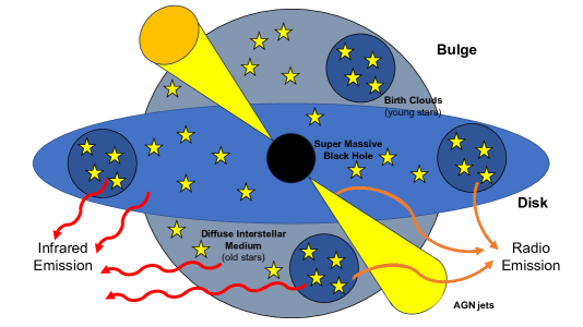
Figure 1: A diagram showing the physics behind the IR and radio emission. IR emission is modelled as in Lagos et al. (2019). UV light from young stars is absorbed by dust and re-emitted at IR wavelengths. Dust is modelled as being in two phases: birth clouds (BC) and diffuse ISM Attenuation dust is modelled using the Charlot & Fall (2000) model, whose parameters depend on galaxy properties. UV light from young stars in BCs are attenuated by both the BCs and ISM, while older stars are only attenuated by the ISM. Radio emission is modelled as a combination of star-formation and AGNs contribution. Radio emission from SF is driven by the presence of young stars (those producing the bulk of the ionising radiation) and from supernovae, both of which are assumed to reside in BCs only. Radio emission by AGNs is driven by the power of jets being a combination of those in the Thin Disk (TD) and Advection Dominated Accretion Flow (ADAF) modes.

Fig. 1 shows a diagram of the physics behind the IR and radio emission in Shark. IR emission is modelled using the method presented in Lagos et al. (2019). The simplest explanation is that IR is the result of UV light being attenuated by dust in birth clouds (BC) and the diffuse Interstellar Medium (ISM), and re-emitted in the IR. The UV light is attenuated using the Charlot & Fall (2000) model with attenuation parameters informed by the radiative transfer analysis of galaxies in the cosmological hydrodynamical simulations Eagle presented in Trayford et al. (2019). This attenuated light is fully re-emitted in the IR following empirical IR templates from Dale et al. (2001). We refer the reader to Lagos et al. (2019) for more details on how the FUV-to-FIR galaxy Spectral Energy Distributions (SEDs) are produced.

Shark uses the ProSpect (Robotham et al., 2020) SED code in its generative mode to produce the synthetic SEDs. ProSpect has the choice of also producing the radio continuum emission associated to star formation, by assuming an underlying IR luminosity to 1.4 GHz continuum luminosity ratio, the spectral indices of the synchrotron and free-free emission and the fraction of the radio continuum that is in the free-free component. This is what was used by Tompkins et al. (2023) to make predictions of the galaxy number counts from $150$ MHz to $8.4$ GHz using Shark. Note that this option in ProSpect can only generate the radio continuum associated to star formation and not AGNs. However, assuming a constant $q_{\rm IR}$ is inflexible and limits the predictive power of Shark. We circumvent this by including in Shark two physical models to compute the radio continuum emission associated to star formation and AGNs, which we describe below.

2.3 Modelling the Radio Emission associated with star formation

Radio emission in B02 is modelled as the sum of the free-free and synchrotron components from each galaxy. Free-free emission is based on the production of ionising photons (as the main source of free electrons) by young and massive stars. Synchrotron emission is modelled from CCSNe which accelerate cosmic ray electrons, making them emit photons at radio frequencies. Supernova remnants also make a minor contribution to synchrotron emission. Below we describe how we model both sources of radio continuum radiation.

2.3.1 Free-Free Radiation

B02 models free-free radiation to be proportional to the production rate of ionising radiation (i.e. Lyman continuum photons) as a proxy for the number of free electrons in the ISM.

The production rate of Lyman continuum photons ($\rm Q_{H}/[s^{-1}]$ ) is calculated as

$$Q_{\rm H}=\int_{0}^{\lambda_{0}}\left(\frac{\lambda L_{\lambda}}{h\,c}\right){\rm d}\lambda,$$ (2)

where $\lambda_{0}$ is the Lyman limit, 921 Å, $\rm L_{\lambda}$ is the galaxy spectrum in $\rm ergs^{-1}$ Å^-1, here $h$ is Planck’s constant (not to be confused with the Hubble parameter of Section 2.1 ) and $c$ is the speed of light. $\rm L_{\lambda}$ is sourced from the galaxy spectrum created using the ProSpect before dust attenuation is applied.

In the process of photo-ionisation of hydrogen, Lyman continuum photons are absorbed. By assuming that the production rate is equal to the destruction rate of Lyman continuum photons, and building off the work of Rubin (1968), Condon (1992) expressed the free-free luminosity in terms of this production rate, HII regions gas temperature, $T$, and frequency, $\nu$, as

$${\frac{L_{\rm ff}}{[\rm W\,Hz^{-1}]}=\frac{Q_{\rm H}}{6.3\times 10^{32}\,\rm[s^{-1}]}\left(\frac{T}{10^{4}\,\rm[K]}\right)^{0.45}\left(\frac{\nu}{\rm[GHz]}\right)^{-0.1}}.$$ (3)

Eq. (3) is used in this paper to calculate the free-free radiation and is identical to that used in O17 (see Ep. 5 in that paper). Note that this equation is of the same form of the equation used to model free-free radiation in B02, but uses a different constant in the denominator of the production rate of Lyman continuum photons; we adopt the same value as O17, $6.3\times 10^{32}s^{-1}$, whereas B02 used $\rm 5.495\times 10^{32}s^{-1}$ (See Equation 1 in B02). B02 used their own simulation model of HII regions to calculate an average relation at 1.49 GHz to find $\rm 5.495\times 10^{32}s^{-1}$. In this paper, we elect to use $\rm 6.3\times 10^{32}s^{-1}$ since it comes from a purely theoretical understanding of free-free radiation. Like B02 and O17, we assume $T=10^{4}\,\rm K$ which aligns with observations of HII regions (Anderson et al. 2009).

2.3.2 Synchrotron Emission

Synchrotron radiation is produced when electrons are accelerated to ultra-relativistic speeds. In the approach of B02, O17 and of this paper the dominant mechanism behind this acceleration is assumed to be CCSNe with a minor contributions from supernova remnants (SNR). Synchrotron radiation is calculated through Eq. (4), which is identical to Eq. (17) in B02:

$$\frac{L_{\rm sync}(\nu)}{10^{23}\,[\rm W\,Hz^{-1}]}=\biggl{[}E_{\rm SNR}\left(\frac{\nu}{1.49\,[\rm GHz]}\right)^{-\alpha_{\rm SNR}}+\\ E_{\rm EI}\left(\frac{\nu}{1.49\,[\rm GHz]}\right)^{-\alpha_{\rm sync}}\biggr{]}\frac{\nu_{\rm CCSN}}{[\rm yr^{-1}]},$$ (4)

where $E_{\rm SNR}$ is the energy contributed by SNRs, $E_{\rm EI}$ is the energy of electrons injected per SN event, $\alpha_{\rm SNR}$ and $\alpha_{\rm sync}$, are the radio luminosity power-law index for the frequency dependence of SNR and of electrons injected per SN event respectively, and $\nu_{\rm CCSNe}$ is the rate of CCSNe.

$\nu_{\rm CCSNe}$ is not assumed to be constant, but instead is calculated from the adopted IMF and the SFR of galaxies,

$$\frac{\nu_{\rm CCSNe}}{{[\rm yr^{-1}]}}=\left(\frac{\alpha_{\rm CCSNe}}{[\rm M_{\odot}^{-1}]}\,\right)\,\left(\frac{\rm SFR}{[\rm M_{\odot}\,yr^{-1}]}\right),$$ (5)

where $\rm\alpha_{CCSNe}$ is the fraction of stars that undergo CCSNe per unit solar mass of stars formed. $\rm\nu_{CCSNe}$ is calculated for each galaxy’s disk and bulge with a galaxy’s total $\rm\nu_{CCSNe}$ being the sum of these two components. It is a common assumption that the stars that eventually undergo CCSNe exist within the mass range of 8 $\rm M_{\odot}\lesssim$ M $\rm\lesssim$ 50 $\rm M_{\odot}$ (Heger et al., 2003; Ando et al., 2003; Nomoto, 1984; Tsujimoto et al., 1997). Above this maximum mass, stars undergo hypernova, causing Gamma Ray Bursts (Van den Heuvel & Yoon 2007). Consequently $\alpha_{\rm CCSNe}$ can be expressed as follows;

$$\alpha_{\rm CCSNe}=\frac{\int_{8\,\rm M_{\odot}}^{50\,\rm M_{\odot}}\psi(M)dM}{\int_{0.1\,\rm M_{\odot}}^{100\,\rm M_{\odot}}M\psi(M)\,{\rm d}M},$$ (6)

where $\rm\psi(M)$ is the IMF. For a Chabrier (2003) IMF this yields $\alpha_{\rm CCSNe}=0.011\rm\,M_{\odot}^{-1}$.

$\rm E^{SNR}$, $\rm E^{EI}$ and $\alpha_{\rm sync}$ are constants and we adopt the values $E_{\rm SNR}=0.0795\times 10^{23}\rm\,W\,Hz^{-1}$, $E_{\rm EI}=1.25\times 10^{23}\rm\,W\,Hz^{-1}$ and $\alpha_{\rm sync}=0.816$. These values are derived empirically and differ from those used in the B02 and O17 due to a different IMF being used in Shark compared to those works. The rest of this subsection is dedicated to the derivation of these constants.

B02 derive the total synchrotron emission in our galaxy using the result of Berkhuijsen (1984). They found the total synchrotron radiation observationally from our Galaxy at 408 MHz to be $L_{\rm MW,0.408GHz}=6.1\times 10^{21}\rm\,W\,Hz^{-1}$. Assuming a radio slope of $\rm\alpha=0.8$ we convert this to the total synchrotron luminosity at 1.49 GHz: $L_{\rm MW,1.49GHz}=2.13\times 10^{21}\,\rm W\,Hz^{-1}$. It is possible to then find the average synchrotron luminosity per supernova event, $E^{\rm sync}$:

$$E^{\rm sync}=\frac{L_{\rm MW,1.49\,GHz}}{\nu_{\rm CCSNe,MW}}=1.24\times 10^{23}\rm\,W\,Hz^{-1},$$ (7)

where $\nu_{\rm CCSN,MW}$ is the rate of CCSNe in the Milky Way. ${\nu_{\rm CCSNe,MW}}$ is assumed to be constant and we adopt ${\nu_{\rm CCSNe}}=0.011\rm\,yr^{-1}$ which is calibrated with the Chabrier IMF used in Shark and uses the same $\alpha_{\rm CCSNe}$ calculated above. B02 and O17 assume ${\nu_{\rm CCSNe}}=0.015\,\rm yr^{-1}$ which comes from Cappellaro & Turatto (2001) and uses a Salpeter (1955) IMF. It is this difference in ${\nu_{\rm CCSNe}}$ that results in the different constants used in this paper compared to those used in B02 and O17.

By assuming that the lifetime of synchrotron electrons is much smaller than the fading time of CCSNe rate (Völk 1989) and that synchrotron radiation is the dominant loss mechanism, B02 shows that the synchrotron luminosity scales linearly with ${\nu_{\rm CCSNe}}$ with a constant $\rm E_{EI}$ for SFGs. This is also true for starbursts; to avoid losses from Inverse Compton scattering, the lifetime of electrons must be shorter in starbursts than in SFGs. On such a short timescale, $\nu_{\rm CCSN,MW}$ can assumed to be constant. B02 also shows that the synchrotron luminosity depends on the magnetic field, $B$, as $\propto B^{\alpha_{\rm sync}-1}$. We follow the same assumption of B02 that $\alpha_{\rm sync}$ is close to $1$ and thus the dependence on $B$ is weak and can be ignored. To quantify this statement, a change in $B$ of a factor of a $100$ (similar to the variations observed in high frequency peaker radio sources by Orienti & Dallacasa 2008 with $B$ in the range $\approx 0.01-0.1$ G) lead to a variation in $L_{\rm sync}$ of a factor $\approx 2$.

The B02 model also considers the contribution of SNRs, noting that other sources provide a negligible contribution. The average SNR synchrotron luminosity per SN event is:

$$E_{\rm SNR}\simeq 0.06E^{\rm sync}.$$ (8)

Eq. (8) tells us that the contribution from SNR makes up about 6 percent of the synchrotron emission. The remaining 94 percent comes from electrons injected into the ISM and accelerated by magnetic fields. As previously derived, $E^{\rm sync}=1.24\times 10^{23}\rm\,W\,Hz^{-1}$ and so $E_{\rm EI}=1.25\times 10^{23}\,\rm W\,Hz^{-1}$, $E_{\rm SNR}=0.0795\times 10^{23}\,\rm W\,Hz^{-1}$.

SNRs have a spectrum which is modelled by $L_{\nu}=\nu^{\alpha_{\rm SNR}}$ where $\alpha_{\rm SNR}=0.2-0.5$. The B02 model assumes that the radio slope of SNRs is constant at $\alpha_{\rm SNR}=0.5$, which is less than the characteristic observed slope of the total non-thermal emission of SFGs ($\rm\alpha_{sync}=0.8$). In order to compensate for this, the B02 model assumes that the spectrum for electrons injected into the ISM has a radio slope of $\alpha_{\rm EI}\simeq 0.9$ for an overall synchrotron radio slope of $\alpha_{\rm sync}=0.8$.

We differ in the approach to radio slopes. Like the B02 model we also assume that $\alpha_{\rm SNR}=0.5$ but use a $\alpha_{\rm EI}=0.816$ since this more accurately produces an overall slope of $\alpha_{\rm sync}=0.8$. This slope gives an overall synchrotron slope of $\alpha_{\rm sync}=0.8$ accounting for the flatter slope from the SNR contribution.

2.4 Modelling the Radio Emission due to AGNs

In modelling the radio luminosities due to AGNs we start with the approach developed in F11 and extend that model to include the effects of synchrotron self-absorption. F11 models AGNs jet power and converts this to a bolometric luminosity and has been used successfully in Griffin et al. (2019) and Amarantidis et al. (2019) to model AGN radio luminosities (the latter successfully modelling using multiple simulation suites including Shark). This model predicts the core jet power, but does not include extended emission (Such emission is only relevant in for very bright sources). We will now give a brief overview of the F11 model and its implementation into Shark, but we refer to the original paper for greater detail.

This model first calculates the power of the radio jets. To do so, the F11 model assumes that both BH spin and the accretion flow influence the power of the radio jet. Blandford & Znajek (1977) showed that the jet power, Q can be approximated by the BH mass ($M_{\rm BH}$), the magnitude of the BH spin ($\rm a$) and the strength of the poloidal magnetic field ($B_{\rm p}$):

$$Q\propto B_{\rm p}^{2}\,M_{\rm BH}^{2}\,a^{2}.$$ (9)

Shark v1.1 assumes that the BH spin parameter is constant at $\rm a=0.67$, as this corresponds to the standard radiation efficiency of $\rm 0.1$ (Bardeen et al., 1972). This assumption of constant BH spin is not realistic; it has been known to evolve with redshift, galaxy morphology and BH mass (Sesana et al., 2014; Izquierdo-Villalba et al., 2020). For that reason, the latest version of Shark (Lagos et al., 2023) self-consistently tracks the development of BH spins, as they merge and accrete matter. We, however, elect to use Shark v1.1 as the FUV-to-FIR emission of galaxies has been investigated in detail (Lagos et al., 2019, 2020), and so instead assume a constant spin. We note that preliminary results of the same AGN radio emission model applied in the new version of Shark produces qualitatively similar radio luminosity functions to what is found with a constant BH spin. However, we leave a full investigation of the results of the radio and FUV-to-FIR emission models in Shark v2.0 for future work.

$B_{\rm p}$ has a dependence on the azimuthal magnetic field strength, $B_{\phi}$ by $B_{\rm p}\approx(\rm H/R)\,B_{\phi}$. $\rm H/R$ is the ratio of BH accretion disk half-thickness to disk radius. This becomes important when considering whether the BH is in thin disk (TD), where $\rm H\ll R$, or advection-dominated accretion flow (ADAF) mode where $\rm H\sim R$ (Heckman & Best 2014). Consequently the power of the jets (summed over both jets) in these two modes are (Meier 2002):

$$Q_{\rm ADAF}=2\times 10^{45}\,{\rm erg\,s^{-1}}\left(\dfrac{M_{\rm BH}}{10^{9}\,\rm M_{\odot}}\right)\left(\dfrac{\dot{m}}{0.01}\right)\,a^{2},$$ (10)

$$Q_{\rm TD}=2\times 10^{43}\,{\rm erg\,s^{-1}}\left(\dfrac{M_{\rm BH}}{10^{9}\,\rm M_{\odot}}\right)^{1.1}\left(\dfrac{\dot{m}}{0.01}\right)^{1.2}\,a^{2},$$ (11)

where $\dot{m}$ is the dimensionless mass accretion rate $\dot{m}=\dot{M}/\dot{M}_{\rm Edd}$. $\dot{M}$ is the accretion rate of the BH of each galaxy as simulated directly in Shark and $\dot{M}_{\rm Edd}$ is the Eddington Accretion rate, $\dot{M}_{\rm Edd}=L_{\rm Edd}/(0.1c^{2})$.

F11 adopts Heinz & Sunyaev (2003) to compute the radio continuum luminosity at a specific frequency from the jet power. This model found that the flux of a jet scales as $M_{\rm BH}^{\xi_{1}}\dot{m}^{\xi_{2}}$ where $\rm\xi_{1}=\xi_{2}=17/12$ for ADAF systems and $\rm\xi_{1}=17/12,\xi_{2}=0$ for radiation-pressure supported systems. Consequently it can be assumed for the luminosities of these two modes that

$$L_{\rm ADAF} \propto (M_{\rm BH}\dot{m})^{1.42},$$ (12)

$$L_{\rm TD} \propto M_{\rm BH}^{1.42}.$$ (13)

Thus the relations in Eqs. 12 and 13 with Eqs. 10 and 11 can be combined such that the exponents of the former remain the same:

$$L_{\rm ADAF}(\nu) = A_{\rm ADAF}\,Q_{\rm ADAF}\left(\dfrac{M_{\rm BH}}{10^{9}\,\rm M_{\odot}}\right)^{0.42}\left(\dfrac{\dot{m}}{0.01}\right)^{0.42}$$ (14)

$$\cdot\left(\frac{\nu}{\rm 1.4\,GHz}\right)^{\alpha_{\rm AGN}},$$

$$L_{\rm TD}(\nu) = A_{\rm TD}\,Q_{\rm TD}\left(\dfrac{M_{\rm BH}}{10^{9}\,\rm M_{\odot}}\right)^{0.32}\left(\dfrac{\dot{m}}{0.01}\right)^{-1.2}$$ (15)

$$\cdot\left(\frac{\nu}{\rm 1.4\,GHz}\right)^{\alpha_{\rm AGN}},$$

where $\rm A_{ADAF}$ and $\rm A_{TD}$ are normalisation coefficients. These are free parameters, and $\alpha_{\rm AGN}$ is the synchrotron power-law, which we set to $=-0.7$. F11 required that $\rm A_{TD}=0.01A_{ADAF}$, $\rm A_{ADAF}=0.05$ for prolonged accretion and $\rm A_{ADAF}=0.07$ for chaotic accretion. Griffin et al. (2019) compared three different sets of $\rm A_{ADAF}$, $\rm A_{TD}$ based on fitting to an AGN RLF at $\rm z=0$ using the GALFORM model of galaxy formation. Amarantidis et al. (2019) take a similar approach with a $\rm\chi^{2}$ minimisation with AGN RLFs over multiple redshifts. For Shark this yielded $A_{\rm ADAF}=1.3\times 10^{-7}$ and $A_{\rm TD}=8.0\times 10^{-3}$. Notably, Amarantidis et al. (2019) found very different results for these normalisation coefficients across different galaxy formation models.

$A_{\rm ADAF}$ and $A_{\rm TD}$ remain free parameters within the radio emission model presented here and there is no correct method of finding them. In this paper we take a hybrid approach by performing a $\rm\chi^{2}$ minimisation procedure when compared with data of AGN RLF at $\rm z=0$ at $\rm 1.4GHz$ from Bonato et al. (2021a); Ceraj et al. (2018); Padovani (2011); Smolčić et al. (2017) (see the left most panel of the middle row in Fig. 3) to find $\rm A_{ADAF}$. We perform this fit is done without considering the effects of synchrotron self-absorption, which has negligible impact at $\rm 1.4GHz$. As Amarantidis et al. (2019) notes, due fewer BHs accreting in the radiative mode at lower redshifts, $\rm A_{TD}$ has little influence on the shape RLF at $\rm z=0$. For this reason we assume that, like F11, $A_{\rm TD}=A_{\rm ADAF}/100$. We avoid taking the same procedure as Amarantidis et al. (2019) since, as we show in Section 3.2, high redshift AGN RLFs are prone to contamination from galaxies dominated by SF.

We adopt values of $A_{\rm ADAF}=1.0\times 10^{-5}$ and $A_{\rm TD}=1.0\times 10^{-7}$.

We extend the F11 model to include an empirical model of the synchrotron self-absorption which is expected to become increasingly important with decreasing frequency. We follow the empirical model of Tingay & De Kool (2003), which characterised the synchrotron self-absorption of the nearby and very well-studied AGN, PKS 1718-649. To do so, they fitted a two component power-law relationship to the observed spectral data of PKS 1718-649, using a $\chi^{2}$ analysis. We adopt this same two-component power-law and the parameters found in Tingay & De Kool (2003):

$$L_{\rm AGN}(\nu) = \sum_{i=1,2}L_{\rm F11}(\nu_{i})\left(\dfrac{\nu}{\nu_{i}}\right)^{-(\beta_{i}-1)/2}\left[\dfrac{1-e^{-\tau_{i},v}}{\tau_{i,v}}\right],$$ (16)

$$\tau_{i,v} = \left(\dfrac{\nu}{\nu_{i}}\right)^{-(\beta_{i}+4)/2},$$ (17)

where $L_{\rm F11}(\nu_{i})=L_{\rm ADAF}(\nu_{i})+L_{\rm TD}(\nu_{i})$ is the luminosity from an AGN as calculated from the F11 model (using Eqs 14 and 15), $\rm\nu_{i}$ is the frequency at which the synchrotron optical depth is 1 and $\rm\beta_{i}$ is the power-law index, and $L_{\rm AGN}$ is the observed AGN luminosity after accounting for synchrotron self-absorption. We adopt the parameters from Tingay & De Kool (2003) that are $\rm v_{1}=1.264$ GHz, $\rm v_{2}=3.249$ GHz, $\rm\beta_{1}=2.204$ and $\rm\beta_{2}=1.905$.

3 Results

In this section we present the results of implementing the radio emission model into Shark. We start with the most general case of radio source number counts (Section 3.1) before increasing in specificity to radio luminosity functions (RLF) (Section 3.2), SFGs (Section 3.3) and (U)LIRGs (Section 3.4). Finally, in Section 3.5 we present the results of investigations into the IRRC and $q_{\rm IR}$’s evolution with redshift and dependence on $\rm M_{*}$. These are all compared with observational results and show that the radio model in Shark is capable of reasonably reproducing these observational results.

3.1 Galaxy number counts in radio frequencies

To compute number counts, we use the Shark lightcone presented in Section 5 of (Lagos et al., 2019), which has an area of $107$ deg² and covers a redshift range $0\leq z\leq 6$. All galaxies with a dummy magnitude (calculated using a stellar mass-to-light ratio of $1$) $<30$ mag are included. We use the properties of the galaxies in the lightcone to compute the radio continuum emission following Sections 2.3 and 2.4. Using Eqn. 4 from Driver & Robotham (2010) with the area and redshift range this lightcone has an approximate cosmic variance of $1.11$%. However, if we only focus on the low-redshift part of the lightcone ($0\leq z\leq 0.25$), cosmic variance is expected to be $\approx 8$%.

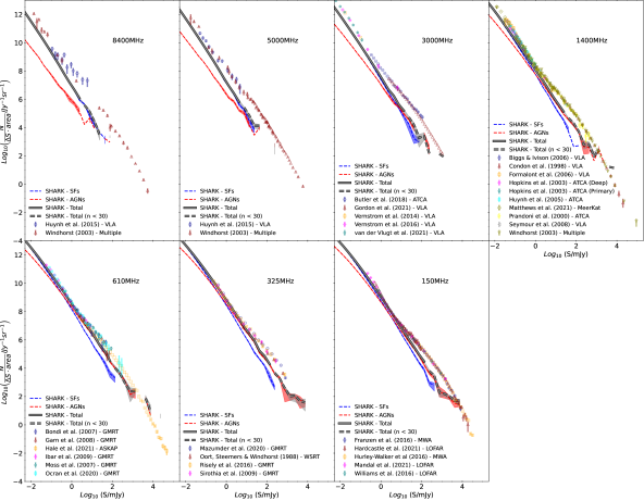
Figure 2: Number counts of galaxies at the labelled frequency. Emission from the Shark SF model (ie the B02 model) is shown in blue and emission from the Shark AGN model (ie the F11 model) is shown in red. The combined total of these two emissions is shown in the thick, grey line, solid grey line shows where the total number of sources is $\rm\geq 30$ and the dashed grey line shows where $\rm<30$. The shaded regions show the $\rm 1-\sigma$ error found using bootstrapping. Data points show counts from different observations from a variety of sources as compiled in Tompkins et al. (2023). This includes data from Huynh et al. (2015); Windhorst (2003) (8400 MHz and 5000 MHz) Butler et al. (2018); Gordon et al. (2021); Vernstrom et al. (2014); Vernstrom et al. (2016); Van der Vlugt et al. (2021) (3000 MHz), Biggs & Ivison (2006); Condon et al. (1998); Hopkins et al. (2003); Huynh et al. (2005); Matthews et al. (2021); Prandoni et al. (2000); Seymour et al. (2008); Windhorst (2003) (1400 MHz), Bondi et al. (2007); Garn et al. (2008); Hale et al. (2021); Ibar et al. (2009); Moss et al. (2007); Ocran et al. (2020) (610 MHz), Mazumder et al. (2020); Oort (1988); Riseley et al. (2016); Sirothia et al. (2009) (325 MHz) and Franzen et al. (2016); Hardcastle et al. (2021); Hurley-Walker et al. (2017); Mandal et al. (2021); Williams et al. (2016) (150 MHz).

Fig. 2 shows the radio source counts for the Shark model compared with observations for frequencies from $\rm 150\,MHz$ to $\rm 8400\,MHz$. The emission solely from SF and AGNs are shown in the dashed lines (blue and red respectively) and their combined total radio emission is shown in the thick grey line. The solid grey line shows where Shark has more than 30 galaxies in the sample and the dashed grey line is where there are fewer than 30 galaxies in the total Shark sample, so is less statistically robust. Errors calculated using bootstrapping are also shown in the shaded regions. Generally, radio source counts can be characterised by the combination of two curves; one dominated by SF and one dominated by AGNs. The intersection of these two curves occurs at brighter fluxes with higher frequencies; SF dominates at $\rm log_{10}(S/mJy)\lesssim 0.75$ at 8400 MHz whereas at 150 MHz this is a order of magnitude fainter at $\rm log_{10}(S/mJy)\lesssim-0.75$. This is not unexpected, as higher frequencies have a smaller synchrotron emission contribution (due to the frequency dependence of the synchrotron emission), requiring ever brighter AGNs to dominate over SF as the frequency increases.

Number counts are compared with observational results compiled by Tompkins et al. (2023) which includes a comprehensive compendium of radio source data from a variety of papers, frequencies and instruments. They also found this two humped distribution where AGNs dominate at the bright end and SF at the faint end. Overall there is a reasonable level of agreement between Shark and the observations. However, there are some tensions and trends that are worth noting. For the purpose of this analysis we define radio faint fluxes as $-2\leq\rm log_{10}(S/mJy)\leq 0$ and radio bright fluxes as $0\leq\rm log_{10}(S/mJy)\leq 2$. We find the difference in between the number counts of the observations and Shark in dex. Here, the relevant number counts for Shark correspond to the total line (summing over the contribution from both SF and AGNs). Note that this difference is calculated for each flux bin, but below we quantify the differences between Shark and observations by computing the median difference in the flux range we define above for faint and bright radio sources.

For faint radio sources, Shark predicts a number of galaxies that is within $1$ dex of what is observed: this difference is greatest at $\rm 8400\,MHz$ of $-0.70$ dex, but this decreases towards lower frequencies with $-0.03$ dex at $\rm 325\,MHz$, and $-0.23$ dex at 150 MHz. We consider Shark to be in reasonable agreement with observations of the number counts of faint radio sources. We therefore conclude that the model of radio emission from SF introduced in Section  2.3 can adequately reproduce the radio source counts in Shark.

A greater source of tension is seen in the radio bright regime. Again across all frequencies Shark predicts fewer objects at fixed flux than observations. This tension is greatest at $8400$ MHz with a difference of $-1.53$ dex and at $5000$ MHz a difference of $-1.06$ dex, but improves at lower frequencies with $-0.28$ dex at $\rm 610\,MHz$, $-0.26$ dex at $\rm 325\,MHz$, and $-0.22$ dex at $\rm 150\,MHz$.

As AGNs dominate the radio bright regime, the tension arises primarily from the model of AGN emission. To understand why the model falls below the observations at the bright end, we studied the redshift distribution of the bright sources in Shark. We focus on the $1.4$ GHz sources as those are the ones we can compare with the RLFs at different redshifts with a range of observations. We find that most of the galaxies with a flux $>100$ mJy in Shark in the lightcone are at $z<0.5$. These are galaxies that have AGN luminosities $>10^{25.5}$ W/Hz. This tension is also apparent in the radio bright regime of the AGN RLF in Fig 3. We discuss this further in Section 3.2.

Two aspects are important to understand why our model leads to an underprediction of the number counts of bright sources in the radio regime. The first one is that the constants $A_{\rm ADAF}$ and $A_{\rm TD}$ used in Eqs. 14 and 15 are calibrated to reproduce intermediate luminosity AGNs in the $\rm 1400\,MHz$ RLF at $z=0$, which is where the constraints are strongest. The second aspect is that in this work extended radio emission is not modelled, which is expected to dominate the flux in galaxies of $1.4$ GHz luminosities $>10^{25}$ W/Hz (e.g. Gendre et al. 2013). Hence, it is not surprising that the number counts fall below the observations at the very bright end. This is something we will revisit once we introduce a model for the extended radio emission of AGNs.

3.2 Radio luminosity functions across cosmic time

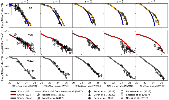
Figure 3: The RLF at 1.4 GHz associated to SF (top panels), to AGNs (middle panels) and the total (bottom panels). Each column is a different redshift from $z=0$ to $4$, as labelled. The shaded regions show the $\rm 1\,\sigma$ error found from bootstrapping. Comparisons are made with observational data of galaxies classified as SFGs in the top panels, AGNs in the middle panels, and the total RLF in the bottom panels; Bonato et al. (2021a), Butler et al. (2019), Novak et al. (2017) and Ocran et al. (2019) (for SFGs), Padovani (2011); Ceraj et al. (2018); Smolčić et al. (2017); Ceraj et al. (2017) for AGNs and Novak et al. (2018) for the total. In the top panels, the blue lines show the true luminosities associated to SF in Shark, while the orange line shows SFGs as identified using the classification from Novak et al. (2017). The difference between the two lines can be attributed to AGN contamination in the latter classification.

We now examine Shark’s performance in reproducing the radio luminosity functions, which is a traditional benchmark to which previous emission models have been compared (Lagos et al. 2019; Somerville et al. 2012; Wilman et al. 2008; Bonaldi et al. 2019; Murphy et al. 2012). We compare Shark results to observations at $\rm 1.4\,GHz$ (Section 3.2.1) and $\rm 150\,MHz$ (Section 3.2.2) and across cosmic time. Note here that these results do not employ the lightcone introduced in Section  3.1; instead using Shark’s native simulated box.

3.2.1 The 1.4 GHz luminosity function

Fig. 3 shows the RLF at 1.4GHz associated to SF in galaxies (top panels), AGNs (middle panels) and the total (bottom panels) across different redshifts.

At $\rm z=0$, Shark compares favourably with the observed data of SFGs and the total radio. By construction Shark will agree well with observations of the AGN RLF at $\rm z=0$ as we used those observations to fit for $\rm A_{ADAF}$. Unlike the AGN RLF at z = 0, the agreement with SFGs and in the total RLF was not guaranteed. This gives us confidence the SF emission model produces reasonable results.

Note that in the AGNs and total RLF, Shark produces too few galaxies brighter than $\rm log_{10}(L_{\rm rad,1.4GHz}/\rm W\,Hz^{-1})\gtrsim 25$. This is related to the tension seen in the predicted number counts in the radio bright regime in Fig.  2. This tension indicates that the AGN luminosity model is under-predicting the number density of very bright AGNs at low redshifts. We attribute this to the lack of extended AGN emission in the model, which dominates AGN emission at $\rm log_{10}(L_{\rm rad,1.4GHz})\gtrsim 25\,\rm WHz^{-1}$ (Gendre et al., 2013). These luminosities are also close to the limit of the simulated box. As there are very few SF galaxies for $\rm log_{10}(L_{\rm rad,1.4GHz})\gtrsim 25\,\rm WHz^{-1}$, the lack of radio bright AGN emission naturally means that the total RLF under-predicts as well at these luminosities.

This good agreement between Shark and the observations continues into the second column for the SF RLF. For AGNs and total this is also true for ${\rm log}_{10}(L_{\rm rad,1.4GHz})\lesssim 26\,\rm WHz^{-1}$.

For the total RLF, there is good agreement with observations at $\rm z=2$ and $z=3$. At $z=4$, however, there is an overabundance of galaxies with $24.5\lesssim\rm log_{10}(L_{\rm rad,1.4GHz}/WHz^{-1})\lesssim 25.5$ in Shark compared to observations, though outside that luminosity range Shark agrees well with observations. The reasonable agreement we get, specially for the total RLF at $1.4\,\rm GHz$ shows that the model performs well even though it has been calibrated at $z=0$ only.

The level of agreement we see in the top and middle panels, however, is not as good as that seen in the bottom panels. At $\rm z\geq 2$ we start to see a persistent under prediction in the RLF associated with SF in galaxies (top panels), and we see the tension with observations increasing from $z=2$ to $z=4$. Note that most of the observations are limited to the range $\rm 25\lesssim log_{10}(L_{rad,1.4GHz}/W\,Hz^{-1})\lesssim 27$. Interestingly, over this same luminosity range, the Shark AGN RLF (middle panels) predicts an over abundance of galaxies compared with observations. At $\rm log_{10}(L_{rad,1.4GHz}/W\,Hz^{-1})\gtrsim 27$, Shark’s predictions for the AGN RLF are in good agreement with observations. The tension seen here is something that is not unique to Shark. Jose et al. (2024) modelled the synchrotron emission of SF galaxies in the semi-analytic model GALFORM and found good agreement with observations for $\rm z<2$, but that the model produced synchrotron luminosities much lower than observations at $\rm z\gtrsim 2$. Below we discuss the tension described here for the RLF of SFGs and AGNs and propose that can be explained in our model by a large fraction of the radio-quiet AGN being mis-classified as SFGs in the observations.

There are numerous caveats to the observations particularly at high redshifts. This includes the underestimation of errors associated with the observations. For each observation we have included the error provided by the papers, however many of these only include Poisson error. This does not account for other sources of error like cosmic variance. Results from Driver & Robotham (2010) estimate the cosmic variance of the area covered by some of these surveys to be as high as $\rm 50\%$. Another caveat is the determination of redshift observationally. These are mostly done using photometry and there is a high probability for catastrophic failure; for example Novak et al. (2018) estimates $\rm\sim 12.5\%$ chance of catastrophic failures at $\rm z\geq 1.5$. The percentage of catastrophic failures is expected to increase with increasing redshift.

Caveats aside, we considered multiple solutions to addressing the tension between the RLFs of SF and AGNs at these high redshifts. One possible option for the tension seen in the top panels for the contribution of SF to the total RLFs could be that the SFRs are too low in Shark. This is not the case and Lagos et al. (2023) in fact showed in their supplementary material (their Fig. 6) that both Shark v1.1 and v2.0 reproduce the observed SFR function from $z=0$ to $z=8$ very well. Another option is that the IMF may be varying, as suggested in other SAMs (Baugh et al., 2005; Lacey et al., 2008; Lacey et al., 2016). We invoked a top-heavy IMF in Shark by post-processing the galaxies to assume different CCSNe rates for SF associated with galaxy disks and starbursts. For disks we continue to assume a Chabrier IMF, but for starbursts we use the top-heavier IMF adopted in Lacey et al. (2016), which gives us $\rm\alpha_{CCSNe}=0.022M_{\odot}^{-1}$ in Eq. (5). Because starbursts are more prevalent at higher redshifts in Shark (Lagos et al. 2018; Lagos et al. 2020), the higher $\rm\alpha_{CCSNe}$ is expected to increase $L_{\rm rad,1.4GHz}$ with increasing redshift. This exercise indeed helps to improve the agreement with observations. However, a full test of this solution would require a varying IMF to be included self-consistently within Shark. In addition, Lagos et al. (2019) found that the UV-to-IR LFs at different cosmic times could be reproduced well by Shark assuming a universal Chabrier IMF, which makes us reluctant to use a varying IMF to reproduce the RLFs.

We also considered cosmic variance as a source of error that could explain this tension. To investigate this we calculated the $\rm 1.4GHz$ RLF but for smaller volumes of the simulated box (specifically volumes of $\rm 5^{3}Mpc^{3}$). While this did increase the error associated with each RLF, it did not bridge the gap between Shark and the observations. We conclude that cosmic variance on its own does not explain the tension in the RLF at $\rm z\sim 3,4$.

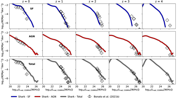
Figure 4: As in Fig. 3 but for $150\,\rm MHz$. Observational results are from Bonato et al. (2021b). We remark that the errorbars associated to the observational datapoints correspond to Poisson uncertainties only.

We propose instead that this tension can be resolved if we consider the way galaxies are selected to be SF or AGNs in observations. Observational studies do not have the luxury of being able to easily distinguish between light purely from AGNs and SF in any one galaxy. Instead observational studies classify galaxies as being either SF or AGN, often in a binary way. This becomes increasingly more difficult to do at higher redshifts as less information (in both the sense of observed radio morphology and the ability to data match with other surveys at different frequencies) is available for these galaxies. Shark is in the comparatively privileged position of not having such limitations, and can also apply the same selections employed in observations to classify galaxies.

Novak et al. (2017) classify and remove radio loud AGNs from their SF RLF using a single criterion first used in Delvecchio et al. (2017) based on a source’s $L_{\rm rad,1.4GHz}$ and SFR to classify it as an AGN:

$${\rm log}_{10}\left(\dfrac{L_{\rm rad,1.4GHz}}{\rm SFR_{IR}}\right)>22\times(1+z)^{0.003}$$ (18)

where $L_{\rm rad,1.4GHz}$ is in units of $\rm W\,Hz^{-1}$ and $\rm SFR_{IR}$ in $\rm M_{\odot}\,yr^{-1}$. We thus take the total RLF in Shark, and remove every Shark galaxy that complies with Eq. (18), irrespective of their individual AGN or SF activity ($L_{\rm rad,1.4GHz}$ used in Eq. 18 is a galaxy’s total radio luminosity with contributions from both SF and AGNs). The remaining would be equivalent to what Novak et al. (2017) report as “SFGs”, and thus would be a fair comparison with their reported RLFs. Note that $\rm SFR_{IR}$ is determined using the SFR-IR relation from Kennicutt Jr (1998). For completeness we derive a galaxy’s $\rm SFR_{IR}$ in the same way in Shark, but note that a similar result is seen if we instead use the intrinsic galaxy’s SFR.

The resulting sample’s RLF is shown by the orange lines in the top panels of Fig. 3. The agreement with the observations is now excellent. This shows that Shark can successfully reproduce observational results when following the same selection method as such observational results, and that it is crucial to attempt to apply the same selection methods as employed in observations to understand how successful Shark is at reproducing observational results.

We speculate that the classification of galaxies into SF/AGN dominated bins would also be responsible for the over abundance in Shark galaxies in the AGN RLF. In high redshift surveys, the sub-mJy population consists of mainly SF-dominated sources, but with some AGN contribution. Empirical AGN diagnostics would classify such sources as solely SF ignoring their composite nature.

3.2.2 The 150 MHz luminosity function

Fig. 4 shows the 150 MHz RLF. We compare with the observational results of Bonato et al. (2021b).

Focusing first on the top left panel of Fig. 4, we see that Shark reproduces well the $\rm z=0$ RLF associated with SFGs. We remind the reader that in the top panels of Fig. 4 we only include the emission associated with SF for the Shark predictions. The predicted normalisation by Shark is a factor of $3$ too high compared with the observed number density at the brightest bin at $\rm log_{10}(L_{rad,150MHz})\sim 24WHz^{-1}$. However, these observations only account for Poisson errorbars and hence are likely very under-estimated, specially at the bright-end (see discussion in Section 3.2.1 about cosmic variance). At higher redshift (top second to fifth panels in Fig. 4), we see similar trends as those discussed for the SF $\rm 1.4GHz$ RLF; Shark predicts an increasingly lower number density than observations of bright galaxies with increasing redshift. Note that observations are only able to constrain the bright-end of the $150\,\rm MHz$ RLF at $z\geq 1$; deeper observations at $150\,\rm MHz$ are needed to measure where the break of the RLF is and the slope below the break. As with $\rm 1.4GHz$, the tension at the bright-end is likely due to contamination from radio-quiet AGNs. Bonato et al. (2021b) use data from Best et al. (2023), which classifies galaxies as AGN-dominated using four different SED fitting methods. The SED modelling applied in Shark only considers the contribution from stars and dust attenuation/re-emission in the FUV-to-FIR, hence we cannot apply the same selection criteria as done in Best et al. (2023) and test for AGN contamination. However, the similarity of the trends here and those presented in Fig. 3 makes us suspect that AGN contamination in the SFGs selection may be an issue here too.

For the AGN RLF (middle panels in Fig. 4) we obtain reasonable agreement between Shark and the observations across different redshifts. The best agreement is at $\rm z=0$, however with increasing redshift we see an opposite trend to that seen in the SF RLF (albeit to a smaller magnitude); Shark predicts a higher number density of bright AGNs at higher luminosities than what is seen in the observational data. This can be seen at $\rm z=1$, where Shark over-predicts compared to the entire observational set, but more evidently at $\rm log_{10}(L_{rad,150MHz})\gtrsim 25WHz^{-1}$. We speculate that this is likely due to the inverse effects of AGN contamination seen in the SF RLF; that the removal of AGNs from the observational data due to their misclassification as SF dominated has lead to the observational data under representing the whole set. Note that we do not see the same tension at radio bright luminosities at $\rm z=0$ for AGNs that is seen in Figs.  2 and  3. There is simply no observational data at $\rm 150MHz$ that probes these high luminosities at this redshift.

The level of agreement between the total RLF and observations is overall better (shown in the bottom panels of Fig. 4), except at the very bright end of each redshift. The better agreement naturally results from the SF contribution being a bit too low and the AGNs one being a bit too high, compensating to some degree. This lends support to our interpretation of the tension in the top and middle panels of Fig. 4 being due to SF/AGN separation difficulties in the observations.

We note that preliminary results obtained using Shark v2.0 (Lagos et al., 2023) show qualitatively similar radio luminosity functions as seen in Figs.  3 and  4, however a full analysis of these results are left for future work.

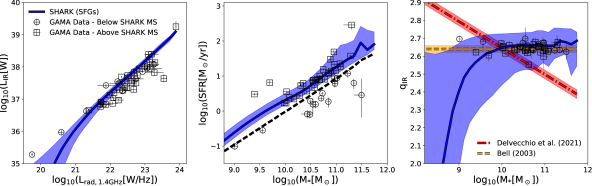
Figure 5: Left panel: The IR-1.4 GHz luminosity relation for SFGs in Shark at $z=0$. The medians and the $16^{\rm th}-84^{\rm th}$ percentile ranges are shown as a line and shaded region, respectively. Symbols show individual GAMA galaxies from the combined GAMA catalogue of (Davies et al., 2017) (1.4 GHz luminosities come from this catalogue) and Bellstedt et al. (2020) (IR luminosities come from this catalogue). Circles are GAMA galaxies that occur above the Shark MS and squares those that occur below. Middle panel: the SFR-stellar mass plane of SFGs in Shark. Solid line with the shaded region and symbols are as in the left panel. All galaxies above the black dashed line are considered SFGs in Shark (see text for details). Right panel: The $q_{\rm IR}$-stellar mass plane. Solid line with the shaded region and symbols are as in the left panel. The red dot-dashed line shows the $q_{\rm IR}$-stellar mass relationship found in Delvecchio et al. (2021) (Fig. 14 in that paper), while the orange dashed line shows the constant $q_{\rm IR}$ found by Bell (2003).

3.3 Radio continuum scaling relations in the local Universe

We now turn to Shark’s performance with respect to SFGs in the local Universe. To test this we compare with observational results from the Galaxy And Mass Assembly (GAMA) survey (Driver et al. 2022). We select only SFGs as they are thought to be the main population driving the observed IRRC. Note that in this case we only include the radio continuum associated to SF and ignore the AGN contribution. To define our population of SFGs within Shark we first define the main sequence (MS) using a linear fit in the space $\rm log_{10}(SFR)-log_{10}(M_{*})$ for central galaxies with stellar masses between $\rm 9\leq log_{10}(M_{*}/M_{\odot})\leq 10$. These mass limits are chosen to avoid resolution limitations on the lower end, and AGN quenching at the higher end. We define SFGs then as those that have $\rm log_{10}(SFR)$ that is $>-0.3$ dex from the main sequence. The latter is inspired by the main sequence having a scatter of $\rm 0.2-0.3$ dex at $z\approx 0$ in observations (Davies et al. 2019; Popesso et al. 2023) and in simulations (Katsianis et al., 2019; Davies et al., 2019). As in Section  3.2, the Shark sample is not sourced from the lightcone, rather Shark’s native simulation box $\rm z=0$ is used.

Fig. 5 shows three scaling relations connecting the radio continuum emission at $1.4$ GHz with other galaxy properties for SFGs in Shark and observations. The observed data here comes from the GAMA analysis of the $1.4$ GHz luminosity of galaxies presented in Davies et al. (2017), which were sourced from the Faint Images of the Radio Sky at Twenty cm (FIRST) survey (Becker et al. 1995). The IR luminosity comes from the SED fitting analysis of the same galaxies presented in Bellstedt et al. (2020). The latter is defined as the total luminosity that is re-radiated in the IR, which is the same definition used in Shark, and hence are comparable. The data here is for galaxies at $z\leq 0.06$ and thus we compare it with Shark predictions at $z=0$. We show GAMA galaxies that occur above the Shark MS as circles and those that are below as squares (although galaxies below MS are only slightly below).

The left panel of Fig. 5 shows $\rm L_{IR}$ as a function of $L_{\rm rad,1.4GHz}$ (i.e. the IRRC). Both populations agree well with each other despite the measurements being determined in different ways. The scatter seen in the GAMA data is larger than the intrinsic scatter in Shark, but that is not surprising as we have not include any potential errors in obtaining luminosities, and the range of SFRs of GAMA galaxies is larger than that of SFGs in Shark (see middle panel of Fig. 5). The agreement shown here was not guaranteed as the IR and radio luminosities in Shark are modelled independently as described in Section 2.

The left panel of Fig. 5 shows that in Shark the median mostly follows a straight line between $\rm log_{10}(L_{\rm IR})$ and $\rm log_{10}(L_{\rm rad,1.4GHz})$ - however, in low luminosity galaxies, $L_{\rm rad,1.4GHz}\lesssim 10^{21}\,\rm W/Hz$, the trend changes so that there is less $L_{\rm IR}$ per unit $L_{\rm rad,1.4GHz}$ than in brighter galaxies. There are only two GAMA galaxies in that regime, which mostly follow the extrapolation of the trend seen in brighter galaxies. Because of the small number of observations it is hard to establish whether there is tension or not with Shark in the faint regime. We see no discernible difference in the distribution of GAMA galaxies that are above Shark’s MS and those that are below in this panel.

The middle panel of Fig. 5 shows the SFR-$\rm M_{*}$ plane. This plot shows that the GAMA sample used here (which only includes those galaxies with FIRST detections) are good representations of SFGs in Shark. 28.9% of GAMA galaxies fall below the dashed line, which marks our threshold to classify galaxies in Shark as being SFGs. However, these galaxies are only mildly below our MS definition in Shark, and the left and right panels of Fig. 5 shows that effectively they follow the same relations as the galaxies above MS.

The right panel of Fig. 5 shows $q_{\rm IR}$ against stellar mass for SFGs. This panel allows for a relative comparison of different $q_{\rm IR}$ results. GAMA, Bell (2003) and Shark all agree in the stellar mass range $\rm 10^{10}-10^{12}\,\rm M_{\odot}$. This is also the regime where the majority of the data from GAMA and Bell (2003) comes from.

Fig. 5 also shows the $q_{\rm IR}$-stellar mass relation reported by Delvecchio et al. (2021) from a set of observations spanning a wide range of stellar masses and redshifts. The authors concluded that there was very little redshift dependence of the $q_{\rm IR}$-stellar mass relation, so we include it in this figure. There is apparent tension between the data from Shark and local Universe observations with the relation reported in Delvecchio et al. (2021). We do not find the same dependence on stellar mass that Delvecchio et al. (2021) found. We investigate this tension thoroughly in Section 3.5.

There are very few galaxies from GAMA or Bell (2003) with stellar masses $\rm<10^{10}\,\rm M_{\odot}$ so meaningful comparisons with observations cannot be made over this mass range. Below a stellar mass of $10^{10}\,\rm M_{\odot}$, Shark predicts a sharp decrease of $q_{\rm IR}$ with a rapid increase in the scatter of the relation. Some galaxies remain in $q_{\rm IR}\approx 2.6$ as seen from the $84^{\rm th}$ percentile, but the majority have $q_{\rm IR}<2.5$ at a stellar mass $<10^{9}\,\rm M_{\odot}$. This is driven by the modelling of the IR and radio continuum from SF. In Shark, the vast majority of these galaxies have their optical depth dominated by birth clouds rather than the diffuse ISM. The optical depth of BCs depends linearly on the ISM metallicity (see Eq. (6) in Lagos et al. 2019). Overall this means as $\rm Z_{gas}$ drops with $\rm M_{*}$ so does the optical depth resulting in less UV emission being absorbed and re-emitted in the IR. This means that there is less IR luminosity per unit SFR in these low-mass galaxies in Shark. The scatter around the median is driven by some low-mass galaxies still having significant diffuse ISM attenuation (those that are close to $q_{\rm IR}\approx 2.6$) and those with insignificant diffuse ISM attenuation (those with $q_{\rm IR}\ll 2.6$).

In Shark, the attenuation due to the ISM is sampled from the attenuation curves reported by Trayford et al. (2019). The high end of this sampling can result in galaxies having a non-negligible ISM optical depth, up to $\rm\tau_{ISM}\sim 0.15$ at these stellar masses (see Fig. 3 in Lagos et al. 2019) even though their ISM metallicity can be slightly sub-solar, effectively cancelling out the decrease in optical depth in the BCs.

This trend in IR not balanced by a similar decrease in radio emission leading to an overall decrease in $q_{\rm IR}$. The model of radio emission due to SF in Shark is predicated on such radio emission being a perfect tracer of the rate of CCSNe. However, Bell (2003) argued that the linearity of the IRRC is proof that radio emission is not a perfect tracer of radio emission in low-luminosity galaxies. Further Chi & Wolfendale (1990) suggested that escape of cosmic ray electrons in lower mass galaxies can explain the linearity of the IRRC. Such a downturn in $q_{\rm IR}$ as seen in Fig. 5 for Shark is due to the lack of modelling of this escape.

There is an overall lack of comprehensive observational data at the stellar masses to which this effect becomes significant. Hence, at this stage we leave this as a caveat of our modelling in Shark and stress that the model seems to apply well to galaxies with stellar masses $\gtrsim 10^{9.7}\,\rm M_{\odot}$ and leave it for future work to test the model in the low-mass regime. We note that the latter will be possible in the near future thanks to surveys such as Evolutionary Map of the Universe (EMU; Norris et al. 2021) being carried out with ASKAP, and the VLASS (Lacy et al. 2020).

3.4 Radio continuum scaling relations at high redshift

We now compare the capabilities of Shark with observations of galaxies at $1\lesssim z\lesssim 2.5$. We do this by compared with galaxies classified as being (U)LIRGs. Specifically we compare with the sample presented in Lo Faro et al. (2015). As in the previous section, we only consider the radio continuum associated with SF here.

In Lo Faro et al. (2015) LIRGs are classified as having a flux at $\rm 24\mu\rm m$ ($\rm S_{24\mu m}$) $\sim 0.2-0.5$ mJy at $z=0.76-1.05$. ULIRGs are classified as having $S_{\rm 24\mu m}\sim 0.14-0.55$ mJy at $z=1.75-2.4$. This differs from the usual definition of LIRGs having IR luminosities in the range $\rm 10^{11}-10^{12}L_{\odot}$ and ULIRGs in the range $\rm 10^{12}-10^{13}L_{\odot}$. We adopt the same definition of Lo Faro et al. (2015) for a fair comparison. For this we use the lightcone presented in Lagos et al. (2019) in their Section 5 (the same used in Section 3.1), after applying the radio continuum model presented in this paper.

Fig. 6 shows the IR-radio continuum, SFR-stellar mass and $q_{\rm IR}$-stellar mass relations for LIRGs and ULIRGs. In all panels, LIRGs are shown in green and ULIRGS in purple with the lines showing the median relations and the shaded region the $\rm 1-\sigma$ percentile range of Shark galaxies. Observations of individual galaxies from Lo Faro et al. (2015) are shown with symbols coloured in the same way. The grey line in the left panel of Fig. 6 shows the population of galaxies selected with only the flux limit ($S_{24\mu m}\sim 0.14-0.55$ mJy) from Shark and no redshift selection.

Compared with the observational results from Lo Faro et al. (2015), Shark broadly agrees. Lo Faro et al. (2015) showed that a clear IRRC exists for both LIRGs and ULIRGs and Shark agrees with this result.

In this same panel, for LIRGs in Shark, there appears to be a flattening at the brighter end of the slope ($L_{\rm rad,1.4GHz}\sim 10^{23.25}\,\rm W\,Hz^{-1}$). A similar phenomena appears to be occurring at the faint end for ULIRGs at $L_{\rm rad,1.4GHz}\sim 10^{23.5}\,\rm W\,Hz^{-1}$ where the slope appears steeper than at higher luminosities. These differences in slope are due to the redshift limits imposed on these populations. This is exemplified by the grey line showing all galaxies in Shark within the flux limit. This line bridges the gap between LIRGs and ULIRGs. Hence, this gap and differences in slopes are driven by the specific selection we are applying here to identify LIRGS and ULIRGS.

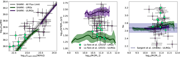
Figure 6: As in Fig. 5 but for LIRGs (green) and ULIRGs (purple) galaxies from Shark (lines with shaded regions) and Lo Faro et al. (2015) (symbols). The right panel also includes the median $q_{\rm IR}$ found for ULIRGs in Sargent et al. (2010b). For Shark, we classify galaxies ad LIRGs and ULIRGs following the same classification adopted in Lo Faro et al. (2015): all galaxies with a $24\,\rm mum$ flux in the range $0.15-0.45$ mJy are selected and those in the redshift ranges $0.76-1.05$ and $1.75-2.4$ are considered LIRGs and ULIRGs, respectively. In the left panel we also show the median and $16^{\rm th}-84^{\rm th}$ percentile ranges for all galaxies in Shark with a $24\,\rm mum$ flux in the range $0.15-0.45$ mJy regardless of their redshift (grey line and shaded region, respectively).

The middle panel of Fig. 6 shows the SFR-stellar mass relation for LIRGs and ULIRGs. The stellar mass of the observed galaxies are determined using SED fits using two different codes: Fadda et al. (2010) use HYPERZ (Bolzonella et al. (2000) while Lo Faro et al. (2013) and Lo Faro et al. (2015) use GRASIL (Silva et al. 1998). The stellar masses shown here were found using HYPERZ (with the difference between the two methods being insignificant).

Fig. 6 shows that the stellar mass ranges of LIRGs and ULIRGs in Lo Faro et al. (2015) are in broad agreement with those found in Shark despite no stellar mass selections in either dataset. Similarly to stellar mass, Lo Faro et al. (2015) use two methods of determining SFR. The first is SED fitting using GRASIL and the other uses the SFR-$\rm L_{IR}$ relation from Kennicutt Jr (1998). We show here the latter estimate. Again, there is broad agreement between Shark and Lo Faro et al. (2015) on the SFRs of both galaxy populations. Although it does appear like the Shark distribution is more bimodal, that stems from the results shown being medians and percentile ranges, rather than individual data points as we show for Lo Faro et al. (2015). The median Shark result is within the margin of error for most of the observations. However is that Shark reproduces well the range of SFRs and stellar masses seen in LIRGs and ULIRGs, and the fact that ULIRGs have on average higher SFRs than LIRGs at fixed stellar mass.

The SFR of ULIRGs in Shark is also nearly half an order of magnitude higher than that observed in Lo Faro et al. (2015). This discrepancy is not necessarily concerning as the sample from Lo Faro et al. (2015) is very small (10 LIRGs and 21 ULIRGs). Lagos et al. (2020) compared the SFRs and stellar masses of sub-mm bright galaxies in Shark with a much larger a complete sample of observed galaxies (of many hundreds), finding that Shark was able to reproduce the observations well within the uncertainties. Therefore it is likely that the discrepancy here is driven by the difficulty in comparing with such a small sample.

The right panel of Fig. 6 shows the dependence of $q_{\rm IR}$ on stellar mass for LIRGs and ULIRGs. In addition to the Lo Faro et al. (2015) data, we also show the median $q_{\rm IR}$ of Sargent et al. (2010b) for ULIRGs as a dotted line. Sargent et al. (2010b) studied 1,692 ULIRGs and 3004 “IR bright” sources out to $\rm z=2$ from the VLA-COSMOS "Joint" Catalogue, and found $q_{\rm IR}=2.672\pm 0.121$ that is independent of redshift. They found no evolution of $q_{\rm IR}$ with redshift but did not test for a possible dependence on $\rm M_{*}$. Shark finds no appreciable dependence of $q_{\rm IR}$ on $\rm M_{*}$ for (U)LIRGs and the median $q_{\rm IR}$ is within the margin of error of that found by Sargent et al. (2010b).

In Shark, LIRGs have a higher median $q_{\rm IR}$ than ULIRGs at the same stellar mass. On the surface, this seems counterintuitive since by definition, ULIRGs have an increased $\rm L_{IR}$ compared with LIRGs. However, as shown in Fig. 6, ULIRGs have an appreciably higher SFR. This SFR leads to an increased $\rm L_{rad,1.4GHz}$ which balances the increased $\rm L_{IR}$ in ULIRGs and results in a similar $q_{\rm IR}$.

In Shark, the ULIRG selection applied here leads to galaxies whose SFR primarily comes from the starburst star formation mode, while LIRGs have a much higher contribution from the disk star formation mode. Shark assumes both SFR modes follow the same relation between the surface density of SFR and molecular gas, except for the normalisation of the burst mode being $10$ times higher than that of the disk mode. The motivation for this was discussed in Lagos et al. (2018) but shortly is inspired by sub-millimeter galaxies having a higher SFR efficiency per unit molecular gas mass than normal star-forming galaxies in observations. Thus, the different modes of star formation can lead to galaxies having different SFR but the same amount of molecular and dust mass, impacting the $L_{\rm IR}-\rm SFR$ relation. This difference in contribution to SFR from starbursts is what leads to a slightly higher $q_{\rm IR}$ (by $0.1$ dex at most) at fixed stellar mass for LIRGs compared to ULIRGs in Shark.

LIRGs with stellar masses $\lesssim 10^{10.5}\,\rm M_{\odot}$ have a higher contribution to their SFR arising from the starburst mode compared with more massive LIRGs. This results in $q_{\rm IR}$ of those lower mass LIRGs being similar to the $q_{\rm IR}$ of ULIRGs in Shark. This transition of the SF mode that dominates the total SFR leads to the weak dependence of $q_{\rm IR}$ on stellar mass for LIRGs that is seen in Shark.

The difference in $q_{\rm IR}$ between LIRGs/ULIRGs was seen in the results of Lo Faro et al. (2015); LIRGs were found to have a higher median $q_{\rm IR}$ than ULIRGs, however a small sample size in that paper meant it was unable to robustly conclude this.

Note that to see the difference between $q_{\rm IR}$ and stellar mass for LIRGs and ULIRGs in Shark would require very large sample sizes for each population in the observations, and precise measurements of $L_{\rm IR}$ and $L_{\rm rad,1.4GHz}$ as to see an average difference of $\approx 0.1$ in $q_{\rm IR}$. This is unattainable with current observations, but the upcoming SKA combined with multi-wavelength observations that allow SED fitting and robust measurements of the IR luminosity, are likely to be sufficient to test the predictions made here.

We also investigated using the usual definition of LIRGs having IR luminosities in the range $\rm 10^{11}-10^{12}L_{\odot}$ and ULIRGs in the range $\rm 10^{12}-10^{13}L_{\odot}$ in Shark, and found no important differences from the results presented here.

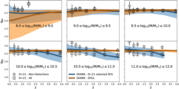
Figure 7: $q_{\rm IR}$ for as a function of redshift for different stellar mass ranges, as labelled. In orange, we show SFGs in Shark as defined in Section 3.3, and considering the radio continuum associated with SF only. In blue, we show the resulting $q_{\rm IR}$ when considering the total radio continuum (coming from both SF and AGNs) and after applying the same galaxy selection as in Delvecchio et al. (2021), whose observations are shown as symbols. Solid lines show the median $q_{\rm IR}$ and the shaded area shows the $\rm 1-\sigma$ percentile range. We show two sets of observations from Delvecchio et al. (2021), median stacked values of non-detections as octagons and the weighted average $q_{\rm IR}$ of detections and non-detections as squares. These two sets should bracket the plausible range of $q_{\rm IR}$ values in the observational sample.

3.5 The IR-radio correlation and its dependence on redshift and stellar mass

We now turn to the IRRC and what Shark can tell us about its evolution with redshift and the influence, if any, that stellar mass has on it. Fig. 7 shows $q_{\rm IR}$ as a function of redshift for different stellar mass ranges for two different ways of selecting Shark SFGs. Orange shows SFGs in Shark (as defined by their distance to the main sequence as described in Section 3.3), and only including radio continuum emission associated with SF; specifically we set each galaxy’s luminosity to that produced solely by the B02 model with no consideration of AGNs. We compare that with the results in blue, which is a population of galaxies in Shark whose radio emission is dominated by SF following the methodology of Delvecchio et al. (2021). In this case, we use the total radio continuum emission of galaxies, which includes both SF and AGNs. As with the results of Sections  3.2 and  3.3, here, we do not employ the lightcone. We compare with the observational results from Delvecchio et al. (2021), which are presented as symbols. The two sets of symbols show the stacked values of non-detections as octagons and the weighted average $q_{\rm IR}$ of detections and non-detections as squares.

The way Delvecchio et al. (2021) identified galaxies dominated by SF in the radio is as follows. A total $q_{\rm IR}$ is calculated from a galaxy’s total radio emission. Then, the main dependence of $q_{\rm IR}$ on redshift is removed by fitting the function $\rm q_{IR}\propto(1+z)^{\alpha}$ and the subtracting the fitted function to the individual $q_{\rm IR}$ values. In effect we are calculating the distance between $q_{\rm IR}$ of individual galaxies and the fitted $\rm q_{IR}\propto(1+z)^{\alpha}$ function. In Delvecchio et al. (2021) this is only done on the two most massive bins (ie $\rm 10.5\leq log_{10}(M/M_{\odot})\leq 11$ and $\rm 11\leq log_{10}(M/M_{\odot})\leq 12$) as these are the mass bins that are most complete. Though we are not limited by this completeness problem, we do the same here to allow for a fair comparison. Having removed the main trend with redshift, a histogram is created of $q_{\rm IR}$ in the two most massive bins (see Fig. 10 in Delvecchio et al. 2021). We then identify the peak or mode of this distribution, $q_{\rm peak}$. It is assumed that this peak and all galaxies with $q_{\rm IR}$ greater than it are dominated by SF and that the distribution is symmetric about $\rm q_{peak}$. In Shark $\rm q_{peak}=2.85$ for both $\rm 10.5\leq log_{10}(M/M_{\odot})\leq 11$ and $\rm 11\leq log_{10}(M/M_{\odot})\leq 12$. We can then take the distribution of galaxies with $q_{\rm IR}>q_{\rm peak}$ and mirror it about $q_{\rm peak}$ and fit a Gaussian to the resulting distribution. From this Gaussian we find $q_{\rm thres}=q_{\rm peak}-2\sigma$ where $\rm\sigma$ is the standard deviation of the fitted Gaussian. In Shark $\rm sigma=0.4$ for $\rm 10.5\leq log_{10}(M/M_{\odot})\leq 11$ and $\rm\sigma=0.35$ for $\rm 11\leq log_{10}(M/M_{\odot})\leq 12$. This is a larger dispersion than that found in Delvecchio et al. (2021) of $0.2$ and $0.23$ respectively. $q_{\rm thres}$ defines the dividing line between SF and AGNs; galaxies with $\rm q_{IR}>q_{\rm thresh}$ are classified as being SFGs and those below are AGN. The method is then repeated, removing more galaxies with $q_{\rm IR}<q_{\rm peak}$ until the median $q_{\rm IR}$ is unchanged within the uncertainties. In Delvecchio et al. (2021) only two iterations are performed before this condition is reached as such we only perform this process twice on Shark galaxies for similar results. The methodology for galaxies with stellar masses $<10^{10.5}\,\rm M_{\odot}$ is the same with one key difference. The $q_{\rm IR}$-redshift function above is extrapolated to lower stellar masses rather than re-fitted.

Having removed AGNs using a similar methodology as Delvecchio et al. (2021), we create the median and $1-\sigma$ percentile range of those Shark galaxies (shown with blue lines and shaded regions in Fig. 7). This is the result that is comparable with the observations reported in Delvecchio et al. (2021). In this comparison we find excellent agreement with Shark in all but a few observational points within the margin of error of the Delvecchio et al. (2021) results. This is quite remarkable given the complexity of both the radio continuum emission model, and the many steps involved in the selection of SFGs. One caveat to this comparison is that the sample used in Delvecchio et al. (2021) is restricted to ’blue’ star forming galaxies defined from their optical colours. In the results presented here we make no such optical identification, but note that we found similar results when such optical identification was included.

Some of the conclusions we can draw from Shark are different though than those drawn by Delvecchio et al. (2021). By putting all the trends shown by the blue lines in Fig. 7, we conclude that the redshift dependence of $q_{\rm IR}$ on redshift is stronger than that on stellar mass in Shark, which is the opposite to what Delvecchio et al. (2021) concluded. The data, however, does agree with Shark within the uncertaintites pointing out that these conclusions are subject to potentially important systematic effects.

The most striking aspect of Fig. 7 is the comparison between the two Shark populations presented. Shark predicts a clear redshift evolution for galaxies with stellar masses in the range $10^{8}-10^{9}\,\rm M_{\odot}$, which is not recovered by the Delvecchio et al. (2021) selection applied to Shark galaxies. This is a consequence of the low $q_{\rm IR}$ galaxies being removed as suspects of AGN contamination. In this case, however, this population of low-mass low $q_{\rm IR}$ galaxies is purely driven by SF, and a result of the modelling included in Shark as described in Section 3.3. At higher stellar masses ($>10^{9}\,\rm M_{\odot}$) Shark the intrinsic $q_{\rm IR}$ (outlined by the orange lines in Fig. 7) show little to no redshift evolution and little stellar mass dependence. In other words, $q_{\rm IR}$ is close to constant (with some scatter) for all galaxies with stellar masses $\gtrsim 10^{9}\,\rm M_{\odot}$. This differs from the picture one could draw from studying the recovered $q_{\rm IR}$ evolution once we apply the method of selecting SFGs in the observations (blue lines in Fig. 7).

The key difference here is the influence of AGNs within the Delvecchio et al. (2021)-selected SFGs. We therefore conclude that the evolution of $q_{\rm IR}$ with z as seen in some observations (e.g Ivison et al. 2010a, b; Magnelli et al. 2015; Delhaize et al. 2017) may largely be driven by AGN contamination from radio-quiet AGNs. We call this “radio-quiet” AGN contamination, because the galaxies that have very bright radio AGN (typically refer to as “radio-loud” AGNs) are the ones that are confidently removed from the galaxy sample once we follow the selection method of Delvecchio et al. (2021).

The conclusion above is very important as it tells us that using $q_{\rm IR}$ in some form to select SFGs, to then measure a $q_{\rm IR}$ may lead to biased results that do not completely remove contaminants. Using independent methods to remove AGNs (ie Cook et al. (2024)) is likely a better choice, though this becomes more difficult to do as we move to samples at high redshift which have less multi-wavelength information from which to independently tag AGNs. This also shows that including all sources of radio continuum emission in Shark is key, even if to evaluate galaxy samples that are dominated by SF given how difficult it is to completely remove the AGN contribution. Finally, the analysis here also shows the importance of following the same selection criteria employed in observations (or at least as closely as possible) to truly assess how well the model performs against observations.

4 Conclusion

We have introduced a model of radio continuum emission associated to SF and AGNs in the semi-analytic model of galaxy formation Shark. We build off the results from Lagos et al. (2019), which successfully modelled the UV-FIR emission using Shark to find the IR emission of galaxies.

We use the approach developed in Bressan et al. (2002) to model emission from SF, which includes synchrotron and free-free emission. Synchrotron is modelled as proportional to the rate of CCSNe with a minor contribution from SNe remnants. Free-free emission is modelled as proportional to the production rate of ionising photons (as a proxy for the number of free electrons).

To model radio emission from AGNs we adopt the Fanidakis et al. (2011) model. This model finds the radio luminosity of AGNs as a function of the power of radio jets. This model depends on the BH mass, accretion rate and spin. The latest version of Shark (Lagos et al., 2023) predicts all these properties for each BH in the simulation, however, for the version of Shark we use here (that of Lagos et al. 2018), only the BH mass and accretion rate are predicted for individual BHs. For the spin we adopt $0.67$, which is equivalent to assuming a standard radiation efficiency of $0.1$.

Below we summarise our main findings and conclusions:

• We show that this model is capable of reproducing a variety of key observations: (i) radio source counts over seven different frequencies from $8.4$ GHz to $150$ MHz (Fig. 2) (to better than $10\%$ in most bands and frequencies and to better than $30$% overall); (ii) the total RLFs at $1.4$ GHz and $150$ MHz from $z=0$ to $z=4$ (bottom panels in Figs. 3 and 4); (iii) the scaling relations between the IR luminosity-$1.4$ GHz luminosity and stellar mass of SFGs in the local universe (Fig. 5) and at high-redshift for LIRGs and ULIRGs (Fig. 6).

• We find that the exact methodology of separating SFGs and AGNs has an impact in the level of agreement we obtain with observations. In particular, we show in Fig 3 that applying the same method that is described in Novak et al. (2017) to separate SFGs and AGNs leads to a good agreement with the RLFs reported there for the two galaxy populations. However, we note that the intrinsic prediction of the contributions to the RLF from SF and AGNs being different to what ends up being associated to either population after applying the method in Novak et al. (2017). This shows that a direct comparison between the intrinsic prediction and the observations would have led us to conclude that poor agreement existed between the two populations.

• We see a similar tension between the $150$ MHz RLFs of SFGs and AGNs reported in observations and the intrinsic prediction in Shark for the contribution to the total RLFs from SF and AGNs. Because the method adopted by Bonato et al. (2021b) to separate SFGs and AGNs at $150$ MHz is more difficult to reproduce (as we lack a model for the mid-IR emission of AGNs in Shark), we do not attempt to do that in this paper, and leave it for future work to assess. However, the results obtained at $1.4$ GHz indicate that AGN contamination needs to be treated carefully when comparing with observations.

• We investigate the relationship between $q_{\rm IR}$, redshift and stellar mass. We first do this by computing $q_{\rm IR}$ for Shark galaxies considering only the radio continuum emission associated with SF. The latter results in no evolution of $q_{\rm IR}$ with redshift and no dependence on $M_{\rm*}$ for galaxies with $M_{\rm*}\gtrsim 10^{9}\,\rm M_{\odot}$. However, if we include the radio continuum emission of AGNs and follow the method of Delvecchio et al. (2021) to remove AGN galaxies, we find that the resulting sample has significant AGN contamination leading to an apparent evolution of $q_{\rm IR}$ with redshift. The resulting $q_{\rm IR}$ agree well with the observations of reported in Delvecchio et al. (2021), but deviate from the intrinsic predictions in Shark for radio continuum associated with SF.

• For galaxies with $M_{\rm*}\lesssim 10^{9}\,\rm M_{\odot}$, Shark predicts a decrease in $q_{\rm IR}$ with decreasing stellar mass and with decreasing redshift. Little observational data exists in that regime, but we note that the likely cause of this in Shark is the lack of a model tracking the relativistic electron escape that is likely to happen in low mass galaxies.

The model for radio continuum emission presented in this paper and implemented in Shark allows the model to extend the wavelength range for SED predictions by orders of magnitude towards the low frequency range, implying an important improvement. We show that this new model is capable of reproducing a variety of observations of galaxies in radio frequencies from the local to the high-redshift Universe RLFs and scaling relations of the radio continuum emission with other galaxy properties. Previous literature focusing on predictions for the radio continuum sky have been done through (semi)-empirical models instead (Wilman et al., 2008; Bonaldi et al., 2019). Our model contributes to the literature by offering a physical model for the radio continuum emission attached to a physical model of galaxy formation and evolution.

This new model extension provides opportunities to investigate the assumptions that are made with respect to how galaxies are selected in radio continuum relative to the emission in other wavelengths and galaxy properties, and it offers a tool for future galaxy surveys to predict the expected properties of the galaxies to be observed given certain flux thresholds.

Data Availability

The SURFS halo and subhalo catalogue and corresponding merger trees used in this work can be accessed from https://tinyurl.com/y6ql46d4. Sharkis a public code and the source and python scripts used to produce the plots in this paper can be found at https://github.com/ICRAR/shark/.

References

- Algera et al. (2020) Algera H., et al., 2020, The Astrophysical Journal, 903, 138
- Amarantidis et al. (2019) Amarantidis S., et al., 2019, Monthly Notices of the Royal Astronomical Society, 485, 2694
- Anderson et al. (2009) Anderson L., Bania T., Jackson J., Clemens D., Heyer M., Simon R., Shah R., Rathborne J., 2009, The Astrophysical Journal Supplement Series, 181, 255
- Ando et al. (2003) Ando S., Sato K., Totani T., 2003, Astroparticle Physics, 18, 307
- Appleton et al. (2004) Appleton P., et al., 2004, The Astrophysical Journal Supplement Series, 154, 147
- Bardeen et al. (1972) Bardeen J. M., Press W. H., Teukolsky S. A., 1972, ApJ, 178, 347
- Baugh et al. (2005) Baugh C., Lacey C. G., Frenk C., Granato G., Silva L., Bressan A., Benson A., Cole S., 2005, Monthly Notices of the Royal Astronomical Society, 356, 1191
- Becker et al. (1995) Becker R. H., White R. L., Helfand D. J., 1995, Astrophysical Journal v. 450, p. 559, 450, 559
- Bell (2003) Bell E. F., 2003, The Astrophysical Journal, 586, 794
- Bellstedt et al. (2020) Bellstedt S., et al., 2020, MNRAS, 498, 5581
- Berkhuijsen (1984) Berkhuijsen E., 1984, Astronomy and Astrophysics, 140, 431
- Best et al. (2023) Best P., et al., 2023, Monthly Notices of the Royal Astronomical Society, p. stad1308
- Biggs & Ivison (2006) Biggs A., Ivison R., 2006, Monthly Notices of the Royal Astronomical Society, 371, 963
- Blandford & Znajek (1977) Blandford R. D., Znajek R. L., 1977, Monthly Notices of the Royal Astronomical Society, 179, 433
- Bolzonella et al. (2000) Bolzonella M., Miralles J.-M., Pelló R., 2000, Arxiv preprint astro-ph/0003380
- Bonaldi (2019) Bonaldi A., 2019, in The Very Large Telescope in 2030. p. 18, doi:10.5281/zenodo.3356246
- Bonaldi et al. (2019) Bonaldi A., Bonato M., Galluzzi V., Harrison I., Massardi M., Kay S., De Zotti G., Brown M. L., 2019, Monthly Notices of the Royal Astronomical Society, 482, 2
- Bonato et al. (2021a) Bonato M., Prandoni I., De Zotti G., Brienza M., Morganti R., Vaccari M., 2021a, Monthly Notices of the Royal Astronomical Society, 500, 22
- Bonato et al. (2021b) Bonato M., et al., 2021b, Astronomy & Astrophysics, 656, A48
- Bondi et al. (2007) Bondi M., et al., 2007, Astronomy & Astrophysics, 463, 519
- Bourne et al. (2011) Bourne N., Dunne L., Ivison R., Maddox S., Dickinson M., Frayer D., 2011, Monthly Notices of the Royal Astronomical Society, 410, 1155
- Bressan et al. (2002) Bressan A., Silva L., Granato G. L., 2002, Astronomy & Astrophysics, 392, 377
- Butler et al. (2018) Butler A., et al., 2018, Astronomy & Astrophysics, 620, A16
- Butler et al. (2019) Butler A., Huynh M., Kapińska A., Delvecchio I., Smolčić V., Chiappetti L., Koulouridis E., Pierre M., 2019, Astronomy & Astrophysics, 625, A111
- Camps et al. (2016) Camps P., Trayford J. W., Baes M., Theuns T., Schaller M., Schaye J., 2016, Monthly Notices of the Royal Astronomical Society, 462, 1057
- Cañas et al. (2019) Cañas R., Elahi P. J., Welker C., Lagos C. d. P., Power C., Dubois Y., Pichon C., 2019, Monthly Notices of the Royal Astronomical Society, 482, 2039
- Cappellaro & Turatto (2001) Cappellaro E., Turatto M., 2001, in , The influence of binaries on stellar population studies. Springer, pp 199–214
- Ceraj et al. (2017) Ceraj L., Smolčić V., Delvecchio I., Delhaize J., Novak M., 2017, Proceedings of the International Astronomical Union, 12, 195
- Ceraj et al. (2018) Ceraj L., et al., 2018, Astronomy & Astrophysics, 620, A192
- Chabrier (2003) Chabrier G., 2003, Publications of the Astronomical Society of the Pacific, 115, 763
- Charlot & Fall (2000) Charlot S., Fall S. M., 2000, The Astrophysical Journal, 539, 718
- Chi & Wolfendale (1990) Chi X., Wolfendale A., 1990, Monthly Notices of the Royal Astronomical Society, 245, 101
- Condon (1992) Condon J., 1992, Annual review of astronomy and astrophysics, 30, 575
- Condon & Ransom (2016) Condon J. J., Ransom S. M., 2016, Essential Radio Astronomy
- Condon et al. (1998) Condon J. J., Cotton W., Greisen E., Yin Q., Perley R. A., Taylor G., Broderick J., 1998, The Astronomical Journal, 115, 1693
- Cook et al. (2024) Cook R. H. W., et al., 2024, arXiv e-prints, p. arXiv:2405.00337
- Dale et al. (2001) Dale D. A., Helou G., Contursi A., Silbermann N. A., Kolhatkar S., 2001, The Astrophysical Journal, 549, 215
- Davies et al. (2017) Davies L. J., et al., 2017, Monthly Notices of the Royal Astronomical Society, 466, 2312
- Davies et al. (2019) Davies L. J. M., et al., 2019, MNRAS, 483, 1881
- De Jong et al. (1985) De Jong T., Klein U., Wielebinski R., Wunderlichº E., 1985, Astron. Astrophys, 147, L6
- Delhaize et al. (2017) Delhaize J., et al., 2017, Astronomy & Astrophysics, 602, A4
- Delvecchio et al. (2017) Delvecchio I., et al., 2017, Astronomy & Astrophysics, 602, A3
- Delvecchio et al. (2021) Delvecchio I., et al., 2021, Astronomy & Astrophysics, 647, A123
- Driver & Robotham (2010) Driver S. P., Robotham A. S., 2010, Monthly Notices of the Royal Astronomical Society, 407, 2131
- Driver et al. (2022) Driver S. P., et al., 2022, Monthly Notices of the Royal Astronomical Society, 513, 439
- Duncan et al. (2020) Duncan K. J., Shivaei I., Shapley A. E., Reddy N. A., Mobasher B., Coil A. L., Kriek M., Siana B., 2020, Monthly Notices of the Royal Astronomical Society, 498, 3648
- Elahi et al. (2018) Elahi P. J., Welker C., Power C., Lagos C. d. P., Robotham A. S., Cañas R., Poulton R., 2018, Monthly Notices of the Royal Astronomical Society, 475, 5338
- Elahi et al. (2019a) Elahi P. J., Cañas R., Poulton R. J., Tobar R. J., Willis J. S., Lagos C. d. P., Power C., Robotham A. S., 2019a, Publications of the Astronomical Society of Australia, 36, e021
- Elahi et al. (2019b) Elahi P. J., Poulton R. J., Tobar R. J., Cañas R., Lagos C. d. P., Power C., Robotham A. S., 2019b, Publications of the Astronomical Society of Australia, 36, e028
- Fadda et al. (2010) Fadda D., et al., 2010, The Astrophysical Journal, 719, 425
- Fanidakis et al. (2011) Fanidakis N., Baugh C., Benson A., Bower R., Cole S., Done C., Frenk C., 2011, Monthly Notices of the Royal Astronomical Society, 410, 53
- Franzen et al. (2016) Franzen T. M., et al., 2016, Monthly Notices of the Royal Astronomical Society, 459, 3314
- Garn et al. (2008) Garn T., Green D. A., Riley J. M., Alexander P., 2008, Monthly Notices of the Royal Astronomical Society, 383, 75
- Gendre et al. (2013) Gendre M. A., Best P. N., Wall J. V., Ker L. M., 2013, MNRAS, 430, 3086
- Giulietti et al. (2022) Giulietti M., et al., 2022, Monthly Notices of the Royal Astronomical Society, 511, 1408
- Gordon et al. (2021) Gordon Y. A., et al., 2021, The Astrophysical Journal Supplement Series, 255, 30
- Griffin et al. (2019) Griffin A. J., Lacey C. G., Gonzalez-Perez V., Lagos C. d. P., 2019, arXiv preprint arXiv:1912.09490
- Hale et al. (2021) Hale C. L., et al., 2021, arXiv preprint arXiv:2109.00956
- Hardcastle et al. (2021) Hardcastle M., et al., 2021, Astronomy & Astrophysics, 648, A10
- Heckman & Best (2014) Heckman T. M., Best P. N., 2014, Annual Review of Astronomy and Astrophysics, 52, 589
- Heger et al. (2003) Heger A., Fryer C. L., Woosley S. E., Langer N., Hartmann D. H., 2003, The Astrophysical Journal, 591, 288
- Heinz & Sunyaev (2003) Heinz S., Sunyaev R., 2003, Monthly Notices of the Royal Astronomical Society, 343, L59
- Helou et al. (1985) Helou G., Soifer B., Rowan-Robinson M., 1985, The Astrophysical Journal, 298, L7
- Hopkins et al. (2003) Hopkins A. M., Afonso J., Chan B., Cram L., Georgakakis A., Mobasher B., 2003, The Astronomical Journal, 125, 465
- Hurley-Walker et al. (2017) Hurley-Walker N., et al., 2017, Monthly Notices of the Royal Astronomical Society, 464, 1146
- Hurley-Walker et al. (2022) Hurley-Walker N., et al., 2022, arXiv preprint arXiv:2204.12762
- Huynh et al. (2005) Huynh M. T., Jackson C. A., Norris R. P., Prandoni I., 2005, The Astronomical Journal, 130, 1373
- Huynh et al. (2015) Huynh M. T., Bell M. E., Hopkins A. M., Norris R. P., Seymour N., 2015, Monthly Notices of the Royal Astronomical Society, 454, 952
- Ibar et al. (2009) Ibar E., Ivison R., Biggs A., Lal D., Best P., Green D., 2009, Monthly Notices of the Royal Astronomical Society, 397, 281
- Ivison et al. (2010a) Ivison R. J., et al., 2010a, Monthly Notices of the Royal Astronomical Society, 402, 245
- Ivison et al. (2010b) Ivison R., et al., 2010b, Astronomy & Astrophysics, 518, L31
- Izquierdo-Villalba et al. (2020) Izquierdo-Villalba D., Bonoli S., Dotti M., Sesana A., Rosas-Guevara Y., Spinoso D., 2020, Monthly Notices of the Royal Astronomical Society, 495, 4681
- Jarvis et al. (2010) Jarvis M. J., et al., 2010, Monthly Notices of the Royal Astronomical Society, 409, 92
- Jarvis et al. (2015) Jarvis M. J., et al., 2015, arXiv preprint arXiv:1412.5753
- Jose et al. (2024) Jose C., Chamandy L., Shukurov A., Subramanian K., Rodrigues L. F. S., Baugh C. M., 2024, Understanding the radio luminosity function of star-forming galaxies and its cosmological evolution (arXiv:2402.15099)
- Katsianis et al. (2019) Katsianis A., et al., 2019, ApJ, 879, 11
- Kennicutt Jr (1998) Kennicutt Jr R. C., 1998, The astrophysical journal, 498, 541
- Kirkpatrick et al. (2013) Kirkpatrick A., et al., 2013, The Astrophysical Journal, 763, 123
- Lacey et al. (2008) Lacey C., Baugh C., Frenk C., Silva L., Granato G., Bressan A., 2008, Monthly Notices of the Royal Astronomical Society, 385, 1155
- Lacey et al. (2016) Lacey C. G., et al., 2016, Monthly Notices of the Royal Astronomical Society, 462, 3854
- Lacy et al. (2016) Lacy M., Baum S. A., Chandler C. J., Chatterjee S., Murphy E. J., Myers S. T., et al., 2016, in American Astronomical Society Meeting Abstracts# 227. pp 324–09
- Lacy et al. (2020) Lacy M., et al., 2020, Publications of the Astronomical Society of the Pacific, 132, 035001
- Lagos et al. (2018) Lagos C. d. P., Tobar R. J., Robotham A. S., Obreschkow D., Mitchell P. D., Power C., Elahi P. J., 2018, Monthly Notices of the Royal Astronomical Society, 481, 3573
- Lagos et al. (2019) Lagos C. d. P., et al., 2019, Monthly Notices of the Royal Astronomical Society, 489, 4196
- Lagos et al. (2020) Lagos C. d. P., Da Cunha E., Robotham A. S., Obreschkow D., Valentino F., Fujimoto S., Magdis G. E., Tobar R., 2020, Monthly Notices of the Royal Astronomical Society, 499, 1948
- Lagos et al. (2023) Lagos C. D. P., et al., 2023, arXiv:2309.0231, p. arXiv:2309.02310
- Lo Faro et al. (2013) Lo Faro B., et al., 2013, The Astrophysical Journal, 762, 108
- Lo Faro et al. (2015) Lo Faro B., Silva L., Franceschini A., Miller N., Efstathiou A., 2015, Monthly Notices of the Royal Astronomical Society, 447, 3442
- Magnelli et al. (2015) Magnelli B., et al., 2015, Astronomy & Astrophysics, 573, A45
- Mancuso et al. (2015) Mancuso C., et al., 2015, The Astrophysical Journal, 810, 72
- Mandal et al. (2021) Mandal S., et al., 2021, Astronomy & Astrophysics, 648, A5
- Mao et al. (2011) Mao M. Y., Huynh M. T., Norris R. P., Dickinson M., Frayer D., Helou G., Monkiewicz J. A., 2011, Proceedings of the International Astronomical Union, 7, 404
- Matthews et al. (2021) Matthews A., Condon J., Cotton W., Mauch T., 2021, The Astrophysical Journal, 909, 193
- Mauch & Sadler (2007) Mauch T., Sadler E. M., 2007, Monthly Notices of the Royal Astronomical Society, 375, 931
- Mazumder et al. (2020) Mazumder A., Chakraborty A., Datta A., Choudhuri S., Roy N., Wadadekar Y., Ishwara-Chandra C., 2020, Monthly Notices of the Royal Astronomical Society, 495, 4071
- Meier (2002) Meier D. L., 2002, New Astronomy Reviews, 46, 247
- Molnár et al. (2021) Molnár D. C., et al., 2021, Monthly Notices of the Royal Astronomical Society, 504, 118
- Morganti et al. (2011) Morganti R., et al., 2011, arXiv preprint arXiv:1112.5094
- Moss et al. (2007) Moss D., Seymour N., McHardy I., Dwelly T., Page M., Loaring N., 2007, arXiv preprint arXiv:0704.2051
- Murphy et al. (2011) Murphy E., et al., 2011, The Astrophysical Journal, 737, 67
- Murphy et al. (2012) Murphy E., et al., 2012, The Astrophysical Journal, 761, 97
- Nomoto (1984) Nomoto K., 1984, The Astrophysical Journal, 277, 791
- Norris et al. (2021) Norris R. P., et al., 2021, Publications of the Astronomical Society of Australia, 38, e046
- Novak et al. (2017) Novak M., et al., 2017, Astronomy & Astrophysics, 602, A5
- Novak et al. (2018) Novak M., Smolčić V., Schinnerer E., Zamorani G., Delvecchio I., Bondi M., Delhaize J., 2018, Astronomy & Astrophysics, 614, A47
- Ocran et al. (2019) Ocran E., Taylor A., Vaccari M., Ishwara-Chandra C., Prandoni I., Prescott M., Mancuso C., 2019, arXiv preprint arXiv:1912.00934
- Ocran et al. (2020) Ocran E., Taylor A., Vaccari M., Ishwara-Chandra C., Prandoni I., 2020, Monthly Notices of the Royal Astronomical Society, 491, 1127
- Omar & Paswan (2018) Omar A., Paswan A., 2018, Monthly Notices of the Royal Astronomical Society, 477, 3552
- Oort (1988) Oort M., 1988, Astronomy and Astrophysics, 192, 42
- Orienti & Dallacasa (2008) Orienti M., Dallacasa D., 2008, A&A, 487, 885
- Padovani (2011) Padovani P., 2011, Monthly Notices of the Royal Astronomical Society, 411, 1547
- Padovani (2017) Padovani P., 2017, Frontiers in Astronomy and Space Sciences, 4, 35
- Panessa et al. (2019) Panessa F., Baldi R. D., Laor A., Padovani P., Behar E., McHardy I., 2019, Nature Astronomy, 3, 387
- Pavlović (2021) Pavlović M., 2021, Serbian Astronomical Journal, pp 15–27
- Popesso et al. (2023) Popesso P., et al., 2023, Monthly Notices of the Royal Astronomical Society, 519, 1526
- Prandoni et al. (2000) Prandoni I., Gregorini L., Parma P., De Ruiter H., Vettolani G., Wieringa M., Ekers R., 2000, Astronomy and Astrophysics Supplement Series, 146, 31
- Riseley et al. (2016) Riseley C., et al., 2016, Monthly Notices of the Royal Astronomical Society, 462, 917
- Robotham et al. (2020) Robotham A., Bellstedt S., Lagos C. d. P., Thorne J., Davies L., Driver S., Bravo M., 2020, Monthly Notices of the Royal Astronomical Society, 495, 905
- Rubin (1968) Rubin R. H., 1968, The Astrophysical Journal, 154, 391
- Salpeter (1955) Salpeter E. E., 1955, The Astrophysical Journal, 121, 161
- Sargent et al. (2010a) Sargent M. T., et al., 2010a, The Astrophysical Journal Supplement Series, 186, 341
- Sargent et al. (2010b) Sargent M. T., et al., 2010b, The Astrophysical Journal Letters, 714, L190
- Sesana et al. (2014) Sesana A., Barausse E., Dotti M., Rossi E. M., 2014, The Astrophysical Journal, 794, 104
- Seymour et al. (2008) Seymour N., et al., 2008, Monthly Notices of the Royal Astronomical Society, 386, 1695
- Shao et al. (2018) Shao L., Koribalski B. S., Wang J., Ho L. C., Staveley-Smith L., 2018, Monthly Notices of the Royal Astronomical Society, 479, 3509
- Shen et al. (2022) Shen X., Vogelsberger M., Nelson D., Tacchella S., Hernquist L., Springel V., Marinacci F., Torrey P., 2022, MNRAS, 510, 5560
- Shimwell et al. (2022) Shimwell T., et al., 2022, Astronomy & Astrophysics, 659, A1
- Silva et al. (1998) Silva L., Granato G. L., Bressan A., Danese L., 1998, The Astrophysical Journal, 509, 103
- Sirothia et al. (2009) Sirothia S., Dennefeld M., Saikia D., Dole H., Ricquebourg F., Roland J., 2009, Monthly Notices of the Royal Astronomical Society, 395, 269
- Smolčić et al. (2017) Smolčić V., et al., 2017, Astronomy & Astrophysics, 602, A1
- Solarz et al. (2019) Solarz A., Pollo A., Bilicki M., Pȩpiak A., Takeuchi T. T., Pia̧tek P., 2019, Publications of the Astronomical Society of Japan, 71, 28
- Somerville et al. (2012) Somerville R. S., Gilmore R. C., Primack J. R., Domínguez A., 2012, Monthly Notices of the Royal Astronomical Society, 423, 1992
- Thomson et al. (2014) Thomson A., et al., 2014, Monthly Notices of the Royal Astronomical Society, 442, 577
- Tingay & De Kool (2003) Tingay S., De Kool M., 2003, The Astronomical Journal, 126, 723
- Tompkins et al. (2023) Tompkins S. A., Driver S. P., Robotham A. S., Windhorst R. A., Lagos C. d. P., Vernstrom T., Hopkins A. M., 2023, Monthly Notices of the Royal Astronomical Society, 521, 332
- Trayford et al. (2017) Trayford J. W., et al., 2017, Monthly Notices of the Royal Astronomical Society, 470, 771
- Trayford et al. (2019) Trayford J. W., Lagos C. d. P., Robotham A. S., Obreschkow D., 2019, arXiv preprint arXiv:1908.08956
- Tsujimoto et al. (1997) Tsujimoto T., Yoshii Y., Nomoto K., Matteucci F., Thielemann F.-K., Hashimoto M., 1997, The Astrophysical Journal, 483, 228
- Van Der Kruit (1973) Van Der Kruit P., 1973, Astronomy and Astrophysics, 29, 263
- Van den Heuvel & Yoon (2007) Van den Heuvel E., Yoon S.-C., 2007, Astrophysics and Space Science, 311, 177
- Van der Kruit (1971) Van der Kruit P., 1971, Astronomy and Astrophysics, Vol. 15, p. 110-122, 15, 110
- Van der Vlugt et al. (2021) Van der Vlugt D., et al., 2021, The Astrophysical Journal, 907, 5
- Vernstrom et al. (2014) Vernstrom T., et al., 2014, Monthly Notices of the Royal Astronomical Society, 440, 2791
- Vernstrom et al. (2016) Vernstrom T., Scott D., Wall J., Condon J., Cotton W., Kellermann K., Perley R., 2016, Monthly Notices of the Royal Astronomical Society, 462, 2934
- Völk (1989) Völk H., 1989, Astronomy and Astrophysics, 218, 67
- Williams et al. (2016) Williams W., et al., 2016, Monthly Notices of the Royal Astronomical Society, 460, 2385
- Wilman et al. (2008) Wilman R., et al., 2008, Monthly Notices of the Royal Astronomical Society, 388, 1335
- Windhorst (2003) Windhorst R. A., 2003, New Astronomy Reviews, 47, 357