A logifold structure on measure spaces

Abstract.

In this paper, we develop a local-to-global and measure-theoretical approach to understand datasets. The idea is to take network models with restricted domains as local charts of datasets. We develop the mathematical foundations for these structures, and show in experiments how it can be used to find fuzzy domains and to improve accuracy in data classification problems.

1. Introduction

Let $X$ be a topological space, $B_{X}$ the corresponding Borel $\sigma$-algebra, and $\mu$ a measure on $(X,B_{X})$. In geometry and topology, the manifold approach dated back to Riemann uses open subsets in $\mathbb{R}^{n}$ as local models to build a space. Such a local-to-global principle is central to geometry and has achieved extremely exciting breakthroughs in modeling spacetime by Einstein’s theory of relativity.

In recent years, the rapid development of data science brings immense interest to datasets that are ‘wilder’ than typical spaces that are well-studied in geometry and topology. Moreover, the development of quantum physics also raises a challenging question of whether the spacetime is a manifold.

Taming the wild is a central theme in the development of mathematics. Advances in computational tools have helped to expand the realm of mathematics in the history. For instance, it took hundreds or thousands of years in human history to recognize irrational numbers and to approximate $\pi$ by rational numbers. From this perspective, we consider machine learning by network models as a modern tool to express a ‘wild space’ as a union (limit) of spaces that admit a finite expression.

From a perspective of small scale, a dataset can be thought as a union of numerous disperse tiny open balls (‘thickened points’). We can regard such a union as a manifold with many contractible components. However, this is useless in applications since this forgets about the relations between different components. In a larger scale, a dataset is a measure space in nature.

We would like to formulate local charts for a measure space that capture more information than contractible balls and that admit finite mathematical expressions. Such an atlas of local charts endows a measure space with an additional geometric structure.

Remark 1.1.

Topological change under different scales is the beautiful subject of persistent homology [ELZ02, ZC05, CZCG05]. Moreover, there are also interesting categorical or sheaf theoretical approaches (see for instance [Cur14, FS19]) to understand relations between different components of a system.

Network models provide a surprisingly successful tool to find mathematical expressions that approximate a dataset. Non-differentiable or even discontinuous functions analogous to logic gate operations are frequently used in network models. It provides an important class of non-smooth and even discontinuous functions to study a space.

In this paper, in place of open subsets of $\mathbb{R}^{n}$, we formulate ‘local charts’ that are closely related to network models and have logic gate interpretations on (fuzzy) measure spaces. The measure of each chart is required to be non-zero. To avoid triviality and requiring too many charts, we may further fix $\epsilon>0$ and require that $\mu(X-U)<\epsilon$ for at least one chart $U$. Such a condition disallows $U$ to be too simple, such as a tiny ball around a data point in $X$. This resembles the Zariski-open condition in algebraic geometry.

We take classification problems as the main motivation. For this, we consider the graph of a function $f:D\to T$, where $D$ is a measurable subset in $\mathbb{R}^{n}$ (with the standard Lebesgue measure), and $T$ is a finite set (with the discrete topology). The graph $\mathrm{gr}(f)\subset D\times T$ is equipped with the push-forward measure by $D\to\mathrm{gr}(f)$.

We will use the graphs of linear logical functions $f:D\to T$ explained below as local models. Then a chart is of the form $(U,\Phi)$, where $U\subset X$ is a measurable subset which satisfies $\mu(X-U)<\epsilon$, and $\Phi:U\to\mathrm{gr}(f)$ is a measure-preserving homeomorphism. We define a linear logifold to be a pair $(X,\mathcal{U})$ where $\mathcal{U}$ is a collection of charts $(U_{i},\Phi_{i})$ such that $\mu(X-\bigcup_{i}U_{i})=0$.

Linear logical functions are motivated from network models and have a logic gate interpretation. A network model consists of a directed graph, whose arrows are equipped with linear functions and vertices are equipped with activation functions, which are typically ReLu or sigmoid functions in middle layers, and are sigmoid or softmax functions in the last layer. Note that sigmoid and softmax functions are smoothings of the discrete-valued step function and the index-max function respectively. The smoothing can be understood as encoding the fuzziness of data.

For the moment, let’s get rid of fuzziness by replacing the sigmoid and softmax functions by step and index-max functions respectively. Then we can build a corresponding linear logical graph for the network. At each node of the graph, there is a system of linear inequalities (on the input Euclidean domain $D\subset\mathbb{R}^{n}$) that produces Boolean outcomes that determine the next node to go for the signal. We call the resulting function to be a linear logical function.

Remark 1.2.

[AJ21] studied relations between neural networks and quiver representations. In [JL23a, JL23b], a network model is formulated as a framed quiver representation; learning of the model was formulated as a stochastic gradient descent over the corresponding moduli space. In this language, we now take several quivers, and we glue their representations together (in a non-linear way) to form a ‘logifold’.

It is interesting to compare the concept developed here with the notion of a quiver stack [LNT23] in an entirely different context, which glues several quiver algebras algebraically to form a ‘noncommutative manifold’. (On the other hand, there was no non-linear activation function involved in quiver stacks.)

It turns out that for $D=\mathbb{R}^{n}$, linear logical functions $\mathbb{R}^{n}\to T$ (where $T$ is identified with a finite subset of $\mathbb{R}$) are equivalent to semilinear functions $\mathbb{R}^{n}\to T$, whose graphs are semilinear sets defined by linear equations and inequalities [vdD99]. Semilinear sets provide the simplest class of definable sets of so-called o-minimal structures [vdD99], which are closely related to model theory in mathematical logic. O-minimal structures made an axiomatic development of Grothendieck’s idea of finding tame spaces that exclude wild topology. On one hand, definable sets have a finite expression which is crucial to the predictive power and interpretability in applications. On the other hand, the setup of measurable sets provide a big flexibility for modeling data.

Approximation by linear logical functions of a measurable function $f:D\to T$, where $D$ is a measurable subset of $\mathbb{R}^{n}$ with $\mu(D)<\infty$, is one of the original motivations.

Theorem 1.3 (Universal approximation theorem by linear logical functions).

Let $f:D\to T$ be a measurable function whose domain $D\subset\mathbb{R}^{n}$ is of finite Lebesgue measure, and suppose that its target set $T$ is finite. For any $\epsilon>0$, there exists a linear logical function $L$ and a measurable set $E\subset\mathbb{R}^{n}$ of the Lebesgue measure less than $\epsilon$ such that $L|_{D-E}\equiv f|_{D-E}$.

By taking the limit $\epsilon\to 0$, the above theorem finds a linear logifold structure on the graph of a measurable function. In reality, $\epsilon$ reflects the error of a network in modeling a dataset.

Compared to more traditional approximation methods, there are reasons why linear logical functions are preferred in many situations. First, when the problem is discrete in nature, it is simple and natural to take the most basic kinds of discrete-valued functions as building blocks. Second, such functions have a network nature which is supported by current computational technology. Third, we can make fuzzy and quantum analogs which have rich meanings in mathematics and physics. In particular, in Section 2.6, we find how averaging in a quantum-classical system leads to non-linear propagation of states.

Figure 1. An example of a logifold. The graph jumps over values $0$ and $1$ infinitely in left-approaching to the point marked by a star (and the length of each interval is halved). This is covered by infinitely many charts of linear logical functions, each of which has only finitely many jumps.

Besides discontinuities, another important element is fuzziness. A fuzzy space is a topological measure space $X$ together with a continuous measurable function $\mathcal{P}:X\to[0,1]$ that encodes the probability of whether a given point belongs to the set. In practice, there is always an ambiguity in determining whether a point belongs to a dataset.

A linear logical function is represented by a directed graph $G$. By equipping each vertex of $G$ a state space and each arrow a continuous map between the state spaces, fuzzy linear logical functions (Definition 2.10) and fuzzy linear logifolds (Definition 3.11) can be naturally defined. In this formulation, the walk on the graph (determined by inequalities) depends on the fuzzy/quantum propagation of the internal state spaces.

Figure 2. The left hand side shows a simple example of a logifold. It is the graph of the step function $[-1,1]\to\{0,1\}$. The figure in the middle shows a fuzzy deformation of it, which is a fuzzy subset in $[-1,1]\times\{0,1\}$. The right hand side shows the graph of probability distribution of quantum observation, which consists of the maps $\frac{|z_{0}|^{2}}{|z_{0}|^{2}+|z_{1}|^{2}}$ and $\frac{|z_{1}|^{2}}{|z_{0}|^{2}+|z_{1}|^{2}}$ from the state space $\mathbb{P}^{1}$ to $\{0,1\}$.

Remark 1.4.

Fuzzy linear logical functions typically appear as smoothings of discrete-valued functions. Families of smoothings of these functions can be studied via non-Archimedean analysis. We plan to elaborate this point in another paper.

In the last section, we explain an implementation of logifold structures on datasets in applications. We combine learning models to a logifold, which is also called to be a model society. Taking the average of several learning models for a given problem is called to be ensemble learning, see for instance [CZ12]. The major new ingredient of our implementation is the fuzzy domain of each model that serves as a chart of the logifold.

A trained model typically does not have a perfect accuracy rate and works well only for a part of the data, or in a subset of classes of the data. A major step here is to find and record the domain of each model where it works well.

In classification problems, a dataset is a fuzzy subset of $\mathbb{R}^{n}\times T$ for a finite set $T=\{c_{1},\ldots,c_{N}\}$ of classes. We restrict the domain of a model to $D\times T^{\prime}$ for some subsets $D\subset\mathbb{R}^{n}$ and $T^{\prime}\subset T$. This means we allow the flexibility of taking ‘partial models’ whose targets are subsets of $T$. In practice, we allow models with ‘coarse targets’ of the form $\{\{c_{1},\ldots,c_{i_{1}}\},\ldots,\{c_{i_{k-1}+1},\ldots,c_{N}\}\}$.

We use certainty scores to find the (fuzzy) scopes of models. In applications, the softmax function in the last layer of each mode produces the certainty scores. For each network model, we restrict the input domain to the subset of data that has certainty scores higher than a threshold. The threshold can be set based on the performance on validation data.

This produces a logifold which has a specific fuzzy domain, namely the union of the fuzzy domains of its charts. In Section 4 and 5, We verify in experiments that this brings a significant improvement in accuracy, especially when the trained models are diverse, or the dataset consists of diverse types of classes whose complexity exceeds the processing power of a single computational model.

Remark 1.5.

In the first sight, it may sound inefficient to train many models for a logifold to tackle a single problem. This is not the case.

First, it is easy to get a lot of models simply by saving the model produced in each epoch of training: in the process of machine learning, each epoch produces a model. The accuracy of many of these models is highly comparable to the best one. Second, there are many efficient methods that turn a trained model into a model of a different structure, such as specialization of targets and migration of domain (see Section 4). Third, logifold allows the reuse of existing trained models, which indeed saves a lot of computational resources.

The experiments and training that we have carried out are relatively in small scale using only 3CPUs and 3GPUs. In this scale, it has already shown advantages of our approach compared to a single model or taking simple average. We hope to test the approach in a larger scale in the near future. Moreover, while we have focused on classification problems, logifold structure is a general notion, and we expect that it will also show advantages in other applications as well, such as graph learning and language learning models.

Acknowledgment

The authors thank to the invaluable support and resources provided by the Boston University Shared Computing Cluster (SCC) for facilitating the experiments conducted in this research.

2. Linear logical functions and their fuzzy analogs

Given a subset of $\mathbb{R}^{n}$, one would like to describe it as the zero locus, the image, or the graph of a function in a certain type. In analysis, we typically think of continuous/smooth/analytic functions. However, when the subset is not open, smoothness may not be the most relevant condition.

The success of network models has taught us a new kind of functions that are surprisingly powerful in describing datasets. Here, we formulate them using directed graphs and call them linear logical functions. First, they have the advantage of being logically interpretable in theory. Second, they are close analogues of quantum processes. Namely, they are made up of linear functions and certain non-linear activation functions, which are analogous to unitary evolution and quantum measurements. Third, it is natural to add fuzziness to these functions and hence they are better adapted to describe statistical data.

2.1. Linear logical functions and their graphs

We consider functions $D\to T$ for $D\subset\mathbb{R}^{n}$ and a finite set $T$ constructed from a graph as follows. Let $G$ be a finite directed graph that has no oriented cycle and has exactly one source vertex which has no incoming arrow and $|T|$ target vertices. Each vertex that has more than one outgoing arrows is equipped with an affine linear function $l=(l_{1},\ldots,l_{k})$ on $\mathbb{R}^{n}$, where the outgoing arrows at this vertex are one-to-one corresponding to the chambers in $\mathbb{R}^{n}$ subdivided by the hyperplanes $\{l_{i}=0\}$. (For theoretical purpose, we define these chambers to contain some of their boundary strata in a way such that they are disjoint and their union equals $\mathbb{R}^{n}$.)

Definition 2.1.

A linear logical function $f_{G,L}:D\to T$ is a function made in the following way from $(G,L)$, where $G$ is a finite directed graph that has no oriented cycle and has exactly one source vertex and $|T|$ target vertices,

$$L=\{l_{v}:v\textrm{ is a vertex with more than one outgoing arrows}\},$$

$l_{v}$ are affine linear functions whose chambers in $D$ are one-to-one corresponding to the outgoing arrows of $v$. $(G,L)$ is called a linear logical graph.

Given $x\in D$, we get a path from the source vertex to one of the target vertices in $G$ as follows. We start with the source vertex. At a vertex, if there is only one outgoing arrow, we simply follow that arrow to reach the next vertex. If there are more than one outgoing arrow, we consider the chambers made by the affine linear function $l$ at that vertex, and pick the outgoing arrow that corresponds to the chamber that $x$ lies in. Since the graph is finite and has no oriented cycle, we will stop at a target vertex, which is associated to an element $t\in T$. This defines the function $f_{G,L}$ by setting $f_{G,L}(x)=t$.

Example 2.2.

Consider a feed-forward network model whose activation function at each hidden layer is the step function, and that at the last layer is the index-max function. The function is of the form

$$\sigma\circ L_{N}\circ s_{N-1}\circ L_{N-1}\circ\ldots\circ s_{1}\circ L_{1}$$

where $L_{i}:\mathbb{R}^{n_{i-1}}\to\mathbb{R}^{n_{i}}$ are affine linear functions with $n_{0}=n$, $s_{i}$ are the entrywise step functions and $\sigma$ is the index-max function. We make the generic assumption that the hyperplanes defined by $L_{2},\ldots,L_{N}$ do not contain the images of $s_{1},\ldots,s_{N-1}$. We claim that this is a linear logical function with target $T=\{1,\ldots,n_{N}\}$ (on any $D\subset\mathbb{R}^{n}$ where $\mathbb{R}^{n}$ is the domain of $L_{1}$).

The linear logical graph $(G,L)$ is constructed as follows. The source vertex $v_{0}$ is equipped with the affine linear function $L_{1}$. Then we make $N$ number of outgoing arrows of $v_{0}$ (and corresponding vertices) where $N$ is the number of chambers of $L_{1}$, which are one-to-one corresponding to the possible outcomes of $s_{1}$ (which form a finite subset of ${\{0,1\}}^{n_{1}}$). Then we consider $s_{2}\circ L_{2}$ restricted to this finite set, which also has a finite number of possible outcomes. This produces exactly one outgoing arrow for each of the vertices in the first layer. We proceed inductively. The last layer $\sigma\circ L_{N}$ is similar and has $n_{N}$ possible outcomes. Thus we obtain $(G,L)$ as claimed, where $L$ consists of only one affine linear function $L_{1}$ over the source vertex. See Figure 3.

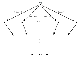
Figure 3.

Example 2.3.

Consider a feed-forward network model whose activation function at each hidden layer is the ReLu function, and that at the last layer is the index-max function. The function takes the form

$$\sigma\circ L_{N}\circ r_{N-1}\circ L_{N-1}\circ\ldots\circ r_{1}\circ L_{1}$$

where $L_{i}:\mathbb{R}^{n_{i-1}}\to\mathbb{R}^{n_{i}}$ are affine linear functions with $n_{0}=n$, $r_{i}$ are the entrywise ReLu functions and $\sigma$ is the index-max function. We construct a linear logical graph $(G,L)$ which produces this function.

The first step is similar to the above example. Namely, the source vertex $v_{0}$ is equipped with the affine linear function $L_{1}$. Next, we make $N$ number of outgoing arrows of $v_{0}$ (and corresponding vertices), where $N$ is the number of chambers of $L_{1}$, which are one-to-one corresponding to the possible outcomes of the sign vector of $r_{1}$ (which form a finite subset of ${\{0,+\}}^{n_{1}}$). Now we consider the next linear function $L_{2}$. For each of these vertices in the first layer, we consider $L_{2}\circ r_{1}\circ L_{1}$ restricted to the corresponding chamber, which is a linear function on the original domain $R^{n}$, and we equip this function to the vertex. Again, we make a number of outgoing arrows that correspond to the chambers in $R^{n}$ made by this linear function. We proceed inductively, and get to the layer of vertices that correspond to the chambers of $L_{N-1}\circ r_{N-2}\circ L_{N-3}\circ\ldots\circ r_{1}\circ L_{1}$. Write $L_{N}=(l_{1},\ldots,l_{n_{N}})$, and consider $\tilde{L}_{N}=(l_{i}-l_{j}:i<j)$. At each of these vertices,

$$\tilde{L}_{N}\circ r_{N-1}\circ L_{N-1}\circ\ldots\circ r_{1}\circ L_{1}$$

restricted on the corresponding chamber is a linear function on the original domain $\mathbb{R}^{n}$, and we equip this function to the vertex and make outgoing arrows corresponding to the chambers of the function. In each chamber, the index $i$ that maximizes $l_{i}\circ r_{N-1}\circ L_{N-1}\circ\ldots\circ r_{1}\circ L_{1}$ is determined, and we make one outgoing arrow from the corresponding vertex to the target vertex $i\in T$. See Figure 4.

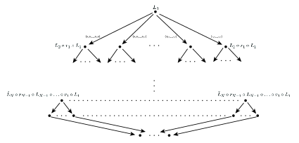
Figure 4.

In classification problems, $T$ is the set of labels for elements in $D$, and the data determines a subset in $D\times T$ as a graph of a function. Deep learning of network models provide a way to approximate the subset as the graph of a linear logical function $\mathrm{gr}(f_{G,L})$. Theoretically, this gives an interpretation of the set, namely, the linear logical graph gives a logical way to deduce the labels based on linear conditional statements on $D$.

The following lemma concerns about the monoidal structure on the set of linear logical functions on $D$.

Lemma 2.4.

Let $f_{G_{i},L_{i}}:D\to T_{i}$ be linear logical functions for $i\in I$ where $I=\{1,\ldots,k\}$. Then

$$(f_{G_{i},L_{i}}:i\in I):D\to\prod_{i\in I}T_{i}$$

is also a linear logical function.

Proof.

We construct a linear logical graph out of $G_{i}$ for $i\in I$ as follows. First, take the graph $G_{1}$. For each target vertex of $G_{1}$, we equip it with the linear function at the source vertex of $G_{2}$, and attach to it the graph $G_{2}$. The target vertices of the resulting graph are labeled by $T_{1}\times T_{2}$. Similarly, each target vertex of this graph is equipped with the linear function at the source vertex of $G_{3}$ and attached with the graph $G_{3}$. Inductively, we obtain the required graph, whose target vertices are labeled by $\prod_{i\in I}T_{i}$. By this construction, the corresponding function is $(f_{G_{i},L_{i}}:i\in I)$. ∎

$f_{(G,L)}$ admits the following algebraic expression in the form of a sum over paths which has an important interpretation in physics. The proof is straightforward and is omitted. A path in a directed graph is a finite sequence of composable arrows. The set of all linear combinations of paths and the trivial paths at vertices form an algebra by concatenation of paths.

Proposition 2.5.

Given a linear logical graph $(G,L)$,

$$f_{(G,L)}(x)=h\left(\sum_{\gamma}c_{\gamma}(x)\,\gamma\right)=\sum_{\gamma}c_{\gamma}(x)\,h(\gamma)$$

where the sum is over all possible paths $\gamma$ in $G$ from the source vertex to one of the target vertices; $h(\gamma)$ denotes the target vertex that $\gamma$ heads to; for $\gamma=a_{r}\ldots a_{1}$,

$$c_{\gamma}(x)=\prod_{i=1}^{r}s_{a_{i}}(x)$$

where $s_{a}(x)=1$ if $x$ lies in the chamber corresponding to the arrow $a$, or $0$ otherwise. In the above sum, exactly one of the terms is non-zero.

2.2. Zero locus

Alternatively, we can formulate the graphs $\mathrm{gr}(f_{G,L})$ as zero loci of linear logical functions targeted at the field $\mathbb{F}_{2}$ with two elements as follows. Such a formulation has the advantage of making the framework of algebraic geometry available in this setting.

Proposition 2.6.

For each linear logical function $f_{G,L}:D\to T$, there exists a linear logical function $f_{\tilde{G},\tilde{L}}:D\times T\to\mathbb{F}_{2}$ whose zero locus in $D\times T$ equals $\mathrm{gr}(f_{G,L})$.

Proof.

Given a linear logical function $f_{G,L}:D\to T$, we construct another linear logical function $f_{\tilde{G},\tilde{L}}:D\times T\to\mathbb{F}_{2}$ as follows. Without loss of generality, let $T=\{1,\ldots,p\}$, so that $D\times T$ is embedded as a subset of $\mathbb{R}^{n+1}$. Any linear function on $\mathbb{R}^{n}$ is pulled back as a linear function on $\mathbb{R}^{n+1}$ by the standard projection $\mathbb{R}^{n+1}\to\mathbb{R}^{n}$ that forgets the last component. Then $f_{G,L}$ is lifted as a linear logical function $D\times T\to T$.

Consider the corresponding graph $(G,L)$. For the $k$-th target vertex of $(G,L)$ (that corresponds to $k\in T$), we equip it with the linear function

$$(y-(k-1/2),(k+1/2)-y):\mathbb{R}^{n+1}\to\mathbb{R}^{2}$$

where $y$ is the last coordinate of $\mathbb{R}^{n+1}$. This linear function produces three chambers in $\mathbb{R}^{n+1}$. Correspondingly we make three outgoing arrows of the vertex. Finally, the outcome vertex that corresponds to $(+,+)$ is connected to the vertex $0\in\mathbb{F}_{2}$; the other two outcome vertices are connected to the vertex $1\in\mathbb{F}_{2}$. We obtain a linear logical graph $(\tilde{G},\tilde{L})$ and the corresponding function $f_{\tilde{G},\tilde{L}}:D\times T\to\mathbb{F}_{2}$.

By construction, $f_{\tilde{G},\tilde{L}}(x,y)=0$ for $(x,y)\in D\times T$ if and only if $y=f_{G,L}(x)\in T$. Thus, the zero locus of $f_{\tilde{G},\tilde{L}}$ is the graph of $f_{G,L}$. ∎

The set of functions (with a fixed domain) valued in $\mathbb{F}_{2}$ forms a unital commutative and associative algebra over $\mathbb{F}_{2}$, which is known as a Boolean algebra.

Proposition 2.7.

The subset of linear logical functions $D\to\mathbb{F}_{2}$ forms a Boolean ring $\mathcal{L}$ (for a fixed $D\subset\mathbb{R}^{n}$).

Proof.

We need to show that the subset is closed under addition and multiplication induced from the corresponding operations of $\mathbb{F}_{2}$.

Let $f_{(G_{1},L_{1})}$ and $f_{(G_{2},L_{2})}$ be linear logical functions $D\to\mathbb{F}_{2}$. By Lemma 2.4, $(f_{(G_{1},L_{1})},f_{(G_{2},L_{2})}):D\to{(\mathbb{F}_{2})}^{2}$ is a linear logical function. Consider the corresponding logical graph. The target vertices are labeled by $(s_{1},s_{2})\in{(\mathbb{F}_{2})}^{2}$. We connect each of them to the vertex $s_{1}+s_{2}\in\mathbb{F}_{2}$ by an arrow. This gives a linear logical graph whose corresponding function is $f_{(G_{1},L_{1})}+f_{(G_{2},L_{2})}$. We obtain $f_{(G_{1},L_{1})}\cdot f_{(G_{2},L_{2})}$ in a similar way. ∎

In this algebro-geometric formulation, the zero locus of $f_{G,L}:D\to\mathbb{F}_{2}$ corresponds to the ideal $(f_{G,L})\subset\mathcal{L}$.

2.3. Parametrization

Another geometric way to describe a set $X$ is via a parametrization $f:D\to X$. This way is commonly used in generative models in machine learning.

The graph $\mathrm{gr}(f_{G,L})$ of a linear logical function can also be put in parametric form. For the moment, let assume the domain $D$ to be finite. First, we need the following lemma.

Lemma 2.8.

Assume $D\subset\mathbb{R}^{n}$ is finite. Then the identity function $I_{D}:D\to D$ is a linear logical function.

Proof.

Since $D$ is finite, there exists a linear function $l:\mathbb{R}^{n}\to\mathbb{R}^{N}$ such that each chamber of $l$ contains at most one point of $D$. Then we construct the linear logical graph $G$ as follows. The source vertex is equipped with the linear function $l$ and outgoing arrows corresponding to the chambers of $l$. Elements of $D$ are identified as the target vertices of these arrows which correspond to chambers that contain them. The corresponding function $f_{G,L}$ equals $I_{D}$. ∎

Proposition 2.9.

Given a linear logical function $f_{G,L}:D\to T$ with finite $|D|$, there exists an injective linear logical function $D\to D\times T$ whose image equals $\mathrm{gr}(f_{G,L})$.

Proof.

By Lemma 2.8 and 2.4, $(I_{D},f_{G,L})$ is a linear logical function. By definition, its image equals $\mathrm{gr}(f_{G,L})$. ∎

2.4. Fuzzy linear logical functions

Another important feature of a dataset is its fuzziness. Below, we formulate the notion of a fuzzy linear logical function and consider its graph.

Definition 2.10.

Let $G$ be a finite directed graph that has no oriented cycle, has exactly one source vertex and target vertices $t_{1},\ldots,t_{K}$ as in Definition 2.1. Each vertex $v$ of $G$ is equipped with a product of standard simplices

$$P_{v}=\prod_{k=1}^{m_{v}}S^{d_{v,k}},\,\,\,S^{d_{v,k}}=\left\{(y_{0},\ldots,y_{d_{v,k}})\in\mathbb{R}_{\geq 0}^{d_{v,k}+1}:\sum_{i=0}^{d_{v,k}}y_{i}=1\right\}$$

for some integers $m_{v}>0$, $d_{v,k}\geq 0$. $P_{v}$ is called the internal state space of the vertex $v$. Let $D$ be a subset of the internal state space of the source vertex of $G$. Each vertex $v$ that has more than one outgoing arrows is equipped with an affine linear function

$$l_{v}:\prod_{k=1}^{m_{v}}\mathbb{R}^{d_{v,k}}\to\mathbb{R}^{j}$$

for some $j>0$, whose chambers in the product simplex $P_{v}$ are one-to-one corresponding to the outgoing arrows of $v$. (In above, $\mathbb{R}^{d_{v,k}}$ is identified with the affine subspace $\left\{\sum_{i=0}^{d_{v,k}}y_{i}=1\right\}$ that contains $S^{d_{v,k}}$.) Let $L$ denote the collection of these linear functions. Moreover, each arrow $a$ is equipped with a continuous function

$$p_{a}:P_{s(a)}\to P_{t(a)}$$

where $s(a),t(a)$ denote the source and target vertices respectively.

We call $(G,L,P,p)$ a fuzzy linear logical graph. $(G,L,P,p)$ determines a function

$$f_{(G,L,P,p)}:D\to P^{\textrm{out}}:=\coprod_{l=1}^{K}P_{t_{l}}$$

as follows. Given $x\in D$, the collection $L$ of linear functions over vertices of $G$ evaluated at the image of $x$ under the arrow maps $p_{a}$ determines a path from the source vertex to one of the target vertices $t_{l}$. By composing the corresponding arrow maps $p_{a}$ on the internal state spaces along the path and evaluating at $x$, we obtain a value $f_{(G,L,P,p)}(x)\in P_{t_{l}}$. The resulting function $f_{(G,L,P,p)}$ is called a fuzzy linear logical function.

Remark 2.11.

Note that the linear functions $l_{v}$ in $L$ in the above definition have domain to be the internal state spaces over the corresponding vertices $v$. In comparison, the linear functions $l_{v}$ in $L$ in Definition 2.1 have domain to be the input space $\mathbb{R}^{n}$. A linear logical graph $(G,L)$ in Definition 2.1 has no internal state space except the $\mathbb{R}^{n}$ at the input vertex.

To relate the two notions given by the above definition and Definition 2.1, we can set $P_{v}=S^{n}$ to be the same for all vertices $v$ except the target vertices $t_{1},\ldots,t_{K}$, which are equipped with the zero-dimensional simplex (a point), and set $p_{a}$ to be identity maps for all arrows $a$ that are not targeted at any of $t_{i}$. Then $f_{(G,L,P,p)}$ reduces back to a linear logical function in Definition 2.1.

We call the corners of the convex set $P_{v}$ to be state vertices, which takes the form $e_{I}=(e_{i_{1}},\ldots,e_{i_{m_{v}}})\in P_{v}$ for a multi-index $I=(i_{1},\ldots,i_{m_{v}})$, where $\{e_{0},\ldots,e_{d_{v,k}}\}\subset\mathbb{R}^{d_{v,k}+1}$ is the standard basis. We can construct a bigger graph by replacing each vertex of $G$ by the collection of state vertices, and each arrow of $G$ by the collection of all possible arrows from source state vertices to target state vertices. Then the vertices of $G$ are interpreted as ‘layers’ or ‘clusters’ of vertices of this bigger graph. The input state $x\in D$, the arrow linear functions $L$ and the maps between state spaces $p$ determine the probability of getting to each target state vertex from the source vertex.

Under this interpretation, we take the target set to be the disjoint union of corners of $P_{t_{l}}$ at the target vertices $t_{1},\ldots,t_{K}$:

(2.1) $$T=\coprod_{l=1}^{K}T_{l}:=\coprod_{l=1}^{K}\left\{e_{I}:I=(i_{1},\ldots,i_{m_{t_{l}}})\textrm{ for }i_{k}\in\{0,\ldots,d_{t_{l},k}\}\right\}$$

which is a finite set. The function $f=f_{(G,L,P,p)}$ determines the probability of the outcome for each input state $x\in D$ as follows. Let $f(x)\in P_{t_{l}}=\prod_{k=1}^{m_{t_{l}}}S^{d_{t_{l},k}}$ for some $l=1,\ldots,K$. Then the probability of being in $T_{j}$ is zero for $j\not=l$. Writing $f(x)=(f_{1}(x),\ldots,f_{m_{t_{l}}}(x))$ for $f_{k}(x)\in S^{d_{t_{l},k}}$, the probability of the output to be $t=e_{I}\in T_{l}$ for $I=(i_{1},\ldots,i_{m_{t_{l}}})$ is given by $\prod_{k=1}^{m_{t_{l}}}f^{(i_{k})}_{k}(x)\in[0,1]$.

Example 2.12.

Consider a feed-forward network model whose activation function at each hidden layer is the sigmoid function $\tilde{s}$, and that at the last layer is the softmax function $\tilde{\sigma}$:

$$f=\tilde{\sigma}\circ L_{N}\circ\tilde{s}_{N-1}\circ L_{N-1}\circ\ldots\circ\tilde{s}_{1}\circ L_{1}.$$

We set $(G,L,P,p)$ as follows. $G$ is the graph that has $(N+1)$ vertices $v_{0},\ldots,v_{N}$ with arrows $a_{i}$ from $v_{i-1}$ to $v_{i}$ for $i=1,\ldots,N$. $L$ is just an empty set. $P_{i}:={(S^{1})}^{m_{i}}$ for $i=0,\ldots,N-1$, where $m_{i}$ is the dimension of the domain of $L_{i+1}$. The one-dimensional simplex $S^{1}$ is identified with the interval $[0,1]$. $P_{N}:=S^{m_{N}}$ where $m_{N}$ is the dimension of the target of $L_{N}$. Then

$$p_{i}:=\tilde{s}_{i}\circ L_{i}|_{{[0,1]}^{m_{i-1}}}\textrm{ for }i=1,\ldots,N-1$$

$$p_{N}:=\tilde{\sigma}\circ L_{N}|_{{[0,1]}^{m_{N-1}}}.$$

Then $f=f_{(G,L,P,p)}$.

Example 2.13.

Consider a feed-forward network model whose activation function at each hidden layer is the ReLu function, and that at the last layer is the softmax function $\tilde{\sigma}$:

$$f=\tilde{\sigma}\circ L_{N}\circ r_{N-1}\circ L_{N-1}\circ\ldots\circ r_{1}\circ L_{1}.$$

We take $G$ to be the logical graph constructed in Example 2.3 (Figure 4) with the last two layers of vertices replaced by a single target vertex $t$. We take the internal state space to be $P_{v}:={(S^{1})}^{n}$ at every vertex $v$ except the target vertex, whose internal state space is defined to be the simplex $P_{t}:=S^{d}$ where $d$ is the target dimension of $L_{N}$. $p_{a}$ is defined to be the identity function for all arrows except those that target at $t$. $L$ is the taken to be the collection of linear functions on $\mathbb{R}^{n}$ over the vertices as in Example 2.3, except the vertices that are adjacent to the last target vertex $t$ and $t$ itself, which do not have more than one outgoing arrows. On each adjacent vertex of the target vertex, recall that $L_{N}\circ r_{N-1}\circ L_{N-1}\circ\ldots\circ r_{1}\circ L_{1}$ restricted on the corresponding chamber is a linear function $l$ on $\mathbb{R}^{n}$. Then $p_{a}$ for the corresponding arrow $a$ is defined to be $\tilde{\sigma}\circ l$. By this construction, we have $f=f_{(G,L,P,p)}$.

As in Proposition 2.5, $f_{(G,L,P,p)}$ can be expressed in the form of sum over paths.

Proposition 2.14.

Given a fuzzy linear logical graph $(G,L,P,p)$,

$$f_{(G,L,P,p)}(x)=\sum_{\gamma}c_{\gamma}(x)\,p_{\gamma}(x)$$

where the sum is over all possible paths $\gamma$ in $G$ from the source vertex to one of the target vertices; for $\gamma=a_{r}\ldots a_{1}$, $p_{\gamma}(x)=\prod_{i=1}^{r}p_{a_{r}}\ldots p_{a_{1}}(x)$;

$$c_{\gamma}(x)=\prod_{i=1}^{r}s_{a_{i}}(p_{a_{i-1}\ldots a_{1}}(x))$$

where $s_{a}(x)=1$ if $x\in P_{t_{a}}$ lies in the chamber corresponding to the arrow $a$, or $0$ otherwise. In the above sum, exactly one of the terms is non-zero.

2.5. As a fuzzy subset

A fuzzy subset of a topological measure space $X$ is a continuous measurable function $\mathcal{F}:X\to[0,1]$. This generalizes the characteristic function of a subset. The interval $[0,1]$ can be equipped with the semiring structure whose addition and multiplication are taking maximum and minimum respectively. This induces a semiring structure on the collection of fuzzy subsets $\mathcal{F}:X\to[0,1]$ that plays the role of union and intersection operations.

The graph $\mathrm{gr}(f)$ of a function

$$f:D\to\coprod_{l=1}^{K}P_{t_{l}},$$

where $P_{t_{l}}$ are products of simplices as in Definition 2.10, is defined to be the fuzzy subset in $D\times T$, where $T$ is defined by Equation (2.1), given by the probability at every $(x,t)\in D\times T$ determined by $f$ in Remark 2.11.

The following is a fuzzy analog of Proposition 2.6.

Proposition 2.15.

Let $f_{(G,L,P,p)}$ be a fuzzy linear logical function. Let $\mathcal{F}:D\times T\to[0,1]$ be the characteristic function of its graph where $T$ is defined by (2.1). Then $\mathcal{F}$ is also a fuzzy linear logical function.

Proof.

Similar to the proof of Proposition 2.6, we embed the finite set $T$ as the subset $\{1,\ldots,|T|\}\subset\mathbb{R}$. The affine linear functions on $\mathbb{R}^{n}\supset D$ in the collection $L$ are pulled back as affine linear functions on $\mathbb{R}^{n+1}\supset D\times T$. Similarly, for the input vertex $v_{0}$, we replace the product simplex $P_{v_{0}}$ by $\tilde{P}_{v_{0}}:=P_{v_{0}}\times[0,|T|+1]$ (where the interval $[0,|T|+1]$ is identified with $S^{1}$); for the arrows $a$ tailing at $v_{0}$, $p_{a}$ are pulled back to be functions $\tilde{P}_{v_{0}}\to P_{h(a)}$. Then we obtain $(\tilde{L},\tilde{P},\tilde{p})$ on $G$.

For each of the target vertices $t_{l}$ of $G$, we equip it with the linear function

$$(y-3/2,y-5/2,\ldots,y-(|T|-1/2)):\mathbb{R}^{n+1}\to\mathbb{R}^{|T|-1}$$

where $y$ is the last coordinate of the domain $\mathbb{R}^{n+1}$. It divides $\mathbb{R}^{n+1}$ into $|T|$ chambers that contain $\mathbb{R}^{n}\times\{j\}$ for some $j=1,\ldots,|T|$. Correspondingly we make $|T|$ outgoing arrows of the vertex $t_{l}$. The new vertices are equipped with the internal state space $P_{t_{l}}$, and the new arrows are equipped with the identity function $P_{t_{l}}\to P_{t_{l}}$. Then we get $|T|K$ additional vertices, where $K$ is the number of target vertices $t_{l}$ of $G$. Let’s label these vertices by $v_{j,l}$ for $j\in T$ and $l\in\{1,\ldots,K\}$. Each of these vertices are connected to the new output vertex by a new arrow. The new output vertex is equipped with the internal state space $S^{1}\cong[0,1]$. The arrow from $v_{j,l}$ to the output vertex is equipped with the following function $p_{j,l}:P_{v_{j,l}}\to[0,1]$. If $j\not\in T_{l}$, then we set $p_{j,l}\equiv 0$. Otherwise, for $j=e_{I}\in T_{l}$ and $I=(i_{1},\ldots,i_{m_{t_{l}}})$, $p_{j,l}:=\prod_{k=1}^{m_{t_{l}}}u^{(i_{k})}_{k}$ where $u_{k}^{(0)},\ldots,u_{k}^{(d_{t_{l},k})}$ are the coordinates of $S^{d_{t_{l},k}}\subset\mathbb{R}_{\geq 0}^{d_{t_{l},k}+1}$. This gives the fuzzy linear logical graph $(\tilde{G},\tilde{L},\tilde{P},\tilde{p})$ whose associated function $f_{(\tilde{G},\tilde{L},\tilde{P},\tilde{p})}:D\times T\to[0,1]$ is the characteristic function. ∎

The above motivates us to consider fuzzy subsets whose characteristic functions are fuzzy linear logical functions $\mathcal{F}:X\to[0,1]$. Below, we will show that they form a sub-semiring, that is, they are closed under fuzzy union and intersection. We will need the following lemma analogous to Lemma 2.4.

Lemma 2.16.

Let $f_{G_{i},L_{i},P_{i},p_{i}}:D\to P^{\textrm{out}}_{i}$ be fuzzy linear logical functions for $i\in I$ where $I=\{1,\ldots,k\}$, and assume that the input state space $P_{i,\mathrm{in}}$ are the same for all $i$. Then

$$(f_{G_{i},L_{i},P_{i},p_{i}}:i\in I):D\to\prod_{i\in I}P^{\textrm{out}}_{i}$$

is also a fuzzy linear logical function.

Proof.

By the proof of Lemma 2.4, we obtain a new graph $(G,L)$ from $(G_{i},L_{i})$ for $i=1,\ldots,k$ by attaching $(G_{i+1},L_{i+1})$ to the target vertices of $(G_{i},L_{i})$. For the internal state spaces, we change as follows. First, we make a new input vertex $\tilde{v}_{0}$ and an arrow $\tilde{a}_{0}$ from $\tilde{v}_{0}$ to the original input vertex $v_{0}$ of $(G,L)$. We denote the resulting graph by $(\tilde{G},\tilde{L})$. We define $\tilde{P}_{\tilde{v}_{0}}:=P_{v_{0}}$, $\tilde{P}_{v_{0}}:=\prod_{i=1}^{k}P_{v_{0}}$ where $P_{v_{0}}=P_{i,\mathrm{in}}$ for all $i$ by assumption, and $\tilde{p}_{\tilde{a}_{0}}:P_{v_{0}}\to\prod_{i=1}^{k}P_{v_{0}}$ to be the diagonal map $\tilde{p}_{\tilde{a}_{0}}=(\mathrm{Id},\ldots,\mathrm{Id})$. The internal state spaces $P_{v}$ over vertices $v$ of $G_{1}$ are replaced by $P_{v}\times\prod_{i=2}^{k}P_{v_{0}}$, and $p_{a}$ for arrows $a$ of $G_{1}$ are replaced by $(p_{a},\mathrm{Id},\ldots,\mathrm{Id})$. Next, over vertices $v$ of the graph $G_{2}$ that is attached to the target vertex $t_{l}$ of $G_{1}$, the internal state space $P_{v}$ is replaced by $P_{t_{l}}\times P_{v}\times\prod_{i=3}^{k}P_{v_{0}}$, and $p_{a}$ for arrows $a$ of $G_{2}$ are replaced by $(\mathrm{Id},p_{a},\mathrm{Id},\ldots,\mathrm{Id})$. Inductively, we obtain the desired graph $(\tilde{G},\tilde{L},\tilde{P},\tilde{p})$. ∎

Proposition 2.17.

Suppose $\mathcal{F}_{1},\mathcal{F}_{2}:X\to[0,1]$ are fuzzy subsets defined by fuzzy linear logical functions. Then $\mathcal{F}_{1}\cup\mathcal{F}_{2}$ and $\mathcal{F}_{1}\cap\mathcal{F}_{2}$ are also fuzzy subsets defined by fuzzy linear logical functions.

Proof.

By the previous lemma, $(\mathcal{F}_{1},\mathcal{F}_{2})=f_{(G,L,P,p)}:X\to[0,1]\times[0,1]$ for some fuzzy linear logical graph $(G,L,P,p)$, which has a single output vertex whose internal state space is $[0,1]\times[0,1]\cong S^{1}\times S^{1}$. We attach an arrow $a$ to this output vertex. Over the new target vertex $v$, $P_{v}:=[0,1]$; $p_{a}:=\max:[0,1]\times[0,1]\to[0,1]$ (or $p_{a}:=\min$). Then we obtain $(\tilde{G},\tilde{L},\tilde{P},\tilde{p})$ whose corresponding fuzzy function defines $\mathcal{F}_{1}\cup\mathcal{F}_{2}$ (or $\mathcal{F}_{1}\cap\mathcal{F}_{2}$ respectively). ∎

Remark 2.18.

For $f:P^{\textrm{in}}\to P^{\textrm{out}}$ where $P^{\textrm{in}},P^{\textrm{out}}$ are product simplices, we can have various interpretations.

1. As a usual function, its graph is in the product $P^{\textrm{in}}\times P^{\textrm{out}}$.

2. As a fuzzy function on $P^{\textrm{in}}$: $P^{\textrm{in}}\to T$ where $T$ is the finite set of vertices of the product simplex $P^{\textrm{out}}$, its graph is a fuzzy subset in $P^{\textrm{in}}\times T$.

3. The domain product simplex $P^{\textrm{in}}$ can also be understood as a collection of fuzzy points over $V$, the finite set of vertices of $P^{\textrm{in}}$, where a fuzzy point here just refers to a probability distribution (which integrates to $1$).

4. Similarly, $P^{\textrm{in}}\times P^{\textrm{out}}$ can be understood as a collection of fuzzy points over $V\times T$. Thus, the (usual) graph of $f$ can be interpreted as a sub-collection of fuzzy points over $V\times T$.

$(\mathrm{Id},f)$ gives a parametric description of the graph of a function $f$. The following ensures that it is a fuzzy linear logical function if $f$ is.

Corollary 2.19.

Let $f:D\to P^{\mathrm{out}}$ be a fuzzy linear logical function. Then $(\mathrm{Id},f):D\to D\times P^{\mathrm{out}}$ is also a fuzzy linear logical function whose image is the graph of $f$.

Proof.

By Lemma 2.16, it suffices to know that $\mathrm{Id}:D\to D$ is a fuzzy linear logical function. This is obvious: we take the graph with two vertices serving as input and output, which are connected by one arrow. The input and output vertices are equipped with the internal state spaces that contain $D$, and $p$ is just defined by the identity function. ∎

Remark 2.20.

Generative deep learning models widely used nowadays can be understood as parametric descriptions of data sets $X$ by fuzzy linear logical functions $f:D\to X$ (where $D$ and $X$ are embedded in certain product simplices $P^{\mathrm{in}}$ and $P^{\mathrm{out}}$ respectively).

2.6. Non-linearity in a quantum-classical system

The fuzzy linear logical functions in Definition 2.10 have the following quantum analog.

Definition 2.21.

Let $G$ be a finite directed graph that has no oriented cycle and has exactly one source vertex and target vertices $t_{1},\ldots,t_{K}$. Each vertex $v$ is equipped with a product of projectifications of Hilbert spaces over complex numbers:

$$Q_{v}:=\prod_{l=1}^{m_{v}}\mathbb{P}(H_{v,l})$$

for some integer $m_{v}>0$. We fix an orthonormal basis in each Hilbert space $H_{v,l}$, which gives a basis in the tensor product:

$$E^{(v)}=\left\{e^{(v)}_{I}=(e^{(v)}_{i_{1}},\ldots,e^{(v)}_{i_{m_{v}}}):e^{(v)}_{i_{l}}\textrm{ is a basic vector of }H_{v,l}\right\}.$$

For each vertex $v$ that has more than one outgoing arrows, we make a choice of a decomposition of the set $E^{(v)}$ into subsets that are one-to-one corresponding to the outgoing arrows. Each arrow $a$ is equipped with a map $q_{a}$ from the corresponding subset of basic vectors $e^{(t(a))}_{I}$ to $Q_{h(a)}$.

Let’s call the tuple $(G,Q,E,q)$ to be a quantum logical graph.

We obtain a probabilistic map $f_{(G,Q,E,q)}:Q^{\mathrm{in}}\to T$ as follows. Given a state $\vec{w}=(w_{1},\ldots,w_{m_{v}})\in Q_{v}$ at a vertex $v$, we make a quantum measurement and $\vec{w}$ projects to one of the basic elements $e^{(v)}_{I}$ with probability $\prod_{l=1}^{m_{v}}|\langle w_{l},e^{(v)}_{i_{l}}\rangle|^{2}$. The outcome $e^{(v)}_{I}$ determines which outgoing arrow $a$ to pick, and the corresponding map $q_{a}$ sends it to an element of $Q_{h(a)}$. Inductively we obtain an element $f_{(G,Q,E,q)}(w)\in T$.

However, such a process is simply linear in probability: the probabilities of outcomes of the quantum process $f_{(G,Q,E,q)}(w)$ for an input state $w$ (which is complex-valued) simply linearly depends on the modulus of components of the input $w$. In other words, the output probabilities are simply obtained by a matrix multiplication on the input probabilities. To produce non-linear physical phenomena, we need the following extra ingredient.

Let’s consider the state space $\mathbb{P}^{n}$ of a single particle. A basis gives a map $\mu:\mathbb{P}^{n}\to S^{n}$ to the simplex $S^{n}$ (also known as the moment map of a corresponding torus action on $\mathbb{P}^{n}$):

$$\mu=\left(\frac{|z_{0}|^{2}}{|z_{0}|^{2}+\ldots+|z_{n}|^{2}},\ldots,\frac{|z_{n}|^{2}}{|z_{0}|^{2}+\ldots+|z_{n}|^{2}}\right):\mathbb{P}^{n}\to S^{n}.$$

The components of the moment map are the probability of quantum projection to basic states of the particle upon observation. By the law of large numbers, if we make independent observations of particles in an identical quantum state $\vec{z}=[z_{0}:\ldots:z_{n}]\in\mathbb{P}^{n}$ for $N$ times, the average of the observed results (which are elements in $\{(1,0,\ldots,0),\ldots,(0,\ldots,0,1)\}$) converges to $\mu(\vec{z})\in S^{n}$ as $N\to\infty$.

The additional ingredient we need is a choice of a map $s:S^{n}\to\mathbb{P}^{m}$ and $m,n\in\mathbb{Z}_{>0}$. For instance, for $m=n=1$, we set the initial phase of the electron spin state according to a number in $[0,1]$.

Upon an observation of a state, we obtain a point in $\{(1,0,\ldots,0),\ldots,(0,\ldots,0,1)\}\subset S^{n}$. Now if we have $N$ particles simultaneously observed, we obtain $N$ values, whose average is again a point $p$ in the simplex $S^{n}$. By $s$, these are turned to $N$ quantum particles in state $s(p)\in\mathbb{P}^{m}$ again.

$\mu:\mathbb{P}^{n}\to S^{n}$ and $s:S^{n}\to\mathbb{P}^{m}$ give an interplay between quantum processes and classical processes with averaging. Averaging in the classical world is the main ingredient to produce non-linearity from the linear quantum process.

Now, let’s modify Definition 2.21 by using $s:S^{n}\to\mathbb{P}^{m}$. Let $P_{v}$ be the product simplex corresponding to $Q_{v}$ at each vertex. Moreover, as in Definition 2.1 and 2.10 for (fuzzy) linear logical functions, we equip each vertex with affine linear functions $l_{v}$ whose corresponding systems of inequalities divide $P_{v}$ into chambers. This decomposition of $P_{v}$ plays the role of the decomposition of $E^{(v)}$ in Definition 2.21. The outgoing arrows at $v$ are in a one-to-one correspondence with the chambers. Each outgoing arrow $a$ at $v$ is equipped with a map $\tilde{q}_{a}$ from the corresponding chamber of $P_{v}$ to $Q_{h(a)}$. $\tilde{q}_{a}$ can be understood as an extension of $q_{a}$ (whose domain is a subset of corners of $P_{t(a)}$) in Definition 2.21.

Definition 2.22.

We call the tuple $(G,Q,E,L,\tilde{q})$ (where $L$ is the collection of affine linear functions $l_{v}$) to be a quantum-classical logical graph.

Given $N$ copies of the same state $\vec{w}$ in $Q_{v}$, we first take a quantum projection of these and they become elements in $P_{v}$. We take an average of these $N$ elements, which lies in a certain chamber defined by $l_{v}$. The chamber corresponds to an outgoing arrow $a$, and the map $\tilde{q}_{a}$ produces $N$ elements in $Q_{h(a)}$. Inductively we obtain a quantum-classical process $Q^{\mathrm{in}}\to T$.

For $N=1$, this essentially produces the same linear probabilistic outcomes as in Definition 2.21. On the other hand, when $N>1$, the process is no longer linear and produces a fuzzy linear logical function $P^{\mathrm{in}}\to P^{\mathrm{out}}$.

In summary, non-linear dependence on the initial state results from averaging of observed states.

Remark 2.23.

We can allow loops or cycles in the above definition. Then the system may run without stop. In this situation, the main object of concern is the resulting (possibly infinite) sequence of pairs $(v,s)$, where $v$ is a vertex of $G$ and $s$ is a state in $Q_{v}$. This gives a quantum-classical walk on the graph $G$.

We can make a similar generalization for (fuzzy) linear logical functions by allowing loops or cycles. This is typical in applications in time-dependent network models.

3. Linear logical structures for a measure space

In the previous section, we have defined linear logical functions based on a directed graph. In this section, we will first show the equivalence between our definition of linear logical functions and semilinear functions[vdD99] in the literature. Thus, the linear logical graph we have defined can be understood as a representation of semilinear functions. Moreover, fuzzy and quantum logical functions that we define can be understood as deformations of semilinear functions.

Next, we will consider measurable functions and show that they can be approximated and covered by semilinear functions. This motivates the definition of a logifold, which is a measure space that has graphs of linear logical functions as local models.

3.1. Equivalence with semilinear functions

Let’s first recall the definition of semilinear sets.

Definition 3.1.

For any positive integer $n$, semilinear sets are the subsets of $\mathbb{R}^{n}$ that are finite unions of sets of the form

(3.1) $$\{x\in\mathbb{R}^{n}:f_{1}(x)=\cdots=f_{k}(x)=0,g_{1}(x)>0,\ldots,g_{l}(x)>0\}$$

where the $f_{i}$ and $g_{j}$ are affine linear functions.

A function $f:D\to T$ on $D\subset\mathbb{R}^{n}$, where $T$ is a discrete set, is called to be semilinear if for every $t\in T$, $f^{-1}\{t\}$ equals to the intersection of $D$ with a semilinear set.

Now let’s consider linear logical functions defined in the last section. We show that the two notions are equivalent (when the target set is finite). Thus, a linear logical graph can be understood as a graphical representation (which is not unique) of a semi-linear function. From this perspective, the last section provides fuzzy and quantum deformations of semi-linear functions.

Theorem 3.2.

Consider $f:D\to T$ for a finite set $T=\{t_{1},\ldots,t_{s}\}$ where $D\subset\mathbb{R}^{n}$. $f$ is a semilinear function if and only if it is a linear logical function.

Proof.

It suffices to consider the case $D=\mathbb{R}^{n}$. We will use the following terminologies for convenience. Let $V(G)$ and $E(G)$ be the sets of vertices and arrows respectively for a directed graph $G$. A vertex $v\in V(G)$ is called to be nontrivial if it has more than one outgoing arrows. It is said to be simple if it has exactly one outgoing arrow. We call a vertex that has no outgoing arrow to be a target, and that has no incoming arrow to be a source. For a target $t$, let $R_{t}$ be the set of all paths from the source to target $t$.

Consider a linear logical function $f=f_{(G,L)}:\mathbb{R}^{n}\to T$. Let $p$ be a path in $R_{t}$ for some $t\in T$. Let $\{v_{1},\ldots,v_{k}\}$ be the set of non-trivial vertices that $p$ passes through. This is a non-empty set unless $f$ is just a constant function (recall that $G$ has only one source vertex). At each of these vertices $v_{i}$, $\mathbb{R}^{n}$ is subdivided according to the affine linear functions $g_{i,1},\ldots,g_{i,N_{i}}$ into chambers $C_{i,1},\ldots,C_{i,m_{i}}$ where $m_{i}$ is the number of its outgoing arrows. All the chambers $C_{i,j}$ are semilinear sets.

For each path $p\in R_{t}$, we define a set $E_{p}$ such that $x\in E_{p}$ if $x$ follows path $p$ to get the target $t$. Then $E_{p}$ can be represented as $C_{1,j_{1}}\cap\cdots\cap C_{k,j_{k}},$ which is semilinear. Moreover, the finite union

$$f^{-1}(t)=\bigcup_{p\in R_{t}}E_{p}$$

is also a semilinear set. This shows that $f$ is a semilinear function.

Conversely, suppose that we are given a semilinear function. Without loss of generality, we can assume that $f$ is surjective. For every $t\in T$, $f^{-1}(t_{i})$ is a semilinear set defined by a collection of affine linear functions in the form of (3.1). Let $\mathcal{F}=\{l_{1},\ldots,l_{N}\}$ be the union of these collections over all $t\in T$.

Now we construct a linear logical graph associated to $f$. We consider the chambers made by $(l_{1},-l_{1},\ldots,l_{N},-l_{N})$ by taking the intersection of the half spaces $l_{i}\geq 0$, $l_{i}<0$, $-l_{i}\geq 0$, $-l_{i}<0$. We construct outgoing arrows of the source vertex associated with these chambers.

For each $t\in T$, $l_{j}$ occurs in defining $f^{-1}(t)$ as either one of the following ways:

1. $l_{j}>0$, which is equivalent to $l_{j}\geq 0$ and $-l_{j}<0$,

2. $l_{j}=0$, which is equivalent to $l_{j}\geq 0$ and $-l_{j}\geq 0$

3. $l_{j}$ is not involved in defining $f^{-1}(t)$.

Thus, $f^{-1}(t)$ is a union of a sub-collection of chambers associated to the outgoing arrows. Then we assign these outgoing arrows with the target vertex $t$. This is well-defined since $f^{-1}(t)$ for different $t$ are disjoint to each other. Moreover, since $\bigcup_{t}f^{-1}(t)=\mathbb{R}^{n}$, every outgoing arrow is associated with a certain target vertex.

In summary, we have constructed a linear logical graph $G$ which produces the function $f$. ∎

The above equivalence between semilinear functions and linear logical functions naturally generalizes to definable functions of other types of $o$-minimal structures. They provide the simplest class of examples in $o$-minimal structures for semialgebraic and subanalytic geometry [vdD99]. Let’s first recall the basic definitions.

Definition 3.3.

[vdD99] A structure $\mathcal{S}$ on $\mathbb{R}$ consists of a Boolean algebra $\mathcal{S}_{n}$ of subsets of $\mathbb{R}^{n}$ for each $n=0,1,2,\ldots,$ such that

1. the diagonals $\{x\in\mathbb{R}^{n}:x_{i}=x_{j}\},1\leq i<j\leq n$ belong to $\mathcal{S}_{n}$;

2. $A\in\mathcal{S}_{m},B\in\mathcal{S}_{n}\implies A\times B\in\mathcal{S}_{m+n}$;

3. $A\in\mathcal{S}_{n+1}\implies\pi(A)\in\mathcal{S}_{n}$, where $\pi:\mathbb{R}^{n+1}\to\mathbb{R}^{n}$ is the projection map defined by $\pi(x_{1},\ldots,x_{n+1})=(x_{1},\ldots,x_{n})$;

4. the ordering $\{(x,y)\in\mathbb{R}^{2}:x<y\}$ of $\mathbb{R}$ belongs to $\mathcal{S}_{2}$.

A structure $\mathcal{S}$ is $o$-minimal if the sets in $\mathcal{S}_{1}$ are exactly the subsets of $\mathbb{R}$ that have only finitely many connected components, that is, the finite unions of intervals and points.

Given a collection $\mathcal{A}$ of subsets of the Cartesian spaces $\mathbb{R}^{n}$ for various $n$, such that the ordering $\{(x,y):x<y\}$ belongs to $\mathcal{A}$, define $\operatorname{Def}(\mathcal{A})$ as the smallest structure on the real line containing $\mathcal{A}$ by adding the diagonals to $\mathcal{A}$ and closing off under Boolean operations, cartesian products and projections. Sets in $\operatorname{Def}(\mathcal{A})$ are said to be definable from $\mathcal{A}$ or just definable if $\mathcal{A}$ is clear from context.

Given definable sets $A\subset\mathbb{R}^{m}$ and $B\subset\mathbb{R}^{n}$ we say that a map $f:A\to B$ is definable if its graph $\Gamma(f)=\{(x,f(x))\in\mathbb{R}^{m+n}:x\in A\}$ is definable.

Remark 3.4.

If $\mathcal{A}$ consist of the ordering, the singletons $\{r\}$ for any $r\in\mathbb{R}$, the graph in $\mathbb{R}^{2}$ of scalar multiplications $x\mapsto\lambda x:\mathbb{R}\to\mathbb{R}$ for any $\lambda\in\mathbb{R}$, and the graph of addition $\{(x,y,z)\in\mathbb{R}^{3}:z=x+y\}$. Then $\operatorname{Def}(\mathcal{A})$ consists of semilinear sets for various positive integer $n$(Definition 3.1).

Similarly, if $\mathcal{A}$ consist of the ordering, singletons, and the graphs of addition and multiplication, then $\operatorname{Def}(\mathcal{A})$ consists of semi-algebraic sets, which are finite unions of sets of the form

$$\left\{x\in\mathbb{R}^{n}:f(x)=0,g_{1}(x)>0,\ldots,g_{l}(x)>0\right\}$$

where $f$ and $g_{1},\ldots,g_{l}$ are real polynomials in $n$ variables, due to the Tarski-Seidenberg Theorem[BM88].

One obtains semi-analytic sets in which the above $f,g_{1},\ldots,g_{l}$ become real analytic functions by including graphs of analytic functions. Let an be the collection $\mathcal{A}$ and of the functions $f:\mathbb{R}^{n}\to\mathbb{R}$ for all positive integer $n$ such that $f|_{I^{n}}$ is analytic, $I=[-1,1]\subset\mathbb{R}$, and $f$ is identically $0$ outside the cubes. The theory of semi-analytic sets and subanalytic sets show that $\operatorname{Def}(\textbf{an})$ is $o$-minimal, and relatively compact semi-analytic sets have only finitely many connected components. See [BM88] for efficient exposition of the Łojasiewicz-Gabrielov-Hironaka theory of semi- and subanalytic sets.

Theorem 3.5.

Let’s replace the collection of affine linear functions at vertices in Definition 2.1 by polynomials and call the resulting functions to be polynomial logical functions. Then $f:D\to T$ for a finite set $T$ is a semi-algebraic function if and only if $f$ is polynomial logical functions.

The proof of the above theorem is similar to that of Theorem 3.2 and hence omitted.

3.2. Approximation of measurable functions by linear logical functions

We consider measurable functions $f:D\to T$, where $0<\mu\left(D\right)<\infty$ and $T$ is a finite set. The following approximation theorem for measurable functions has two distinct features since $T$ is a finite set. First, the functions under consideration, and linear logical functions that we use, are discontinuous. Second, the ‘approximating function’ actually exactly equals to the target function in a large part of $D$. Compared to traditional approximation methods, linear logical functions have an advantage of being representable by logical graphs, which have fuzzy or quantum generalizations.

Theorem 3.6 (Universal approximation theorem for measurable functions).

Let $\mu$ be the standard Lebesgue measure on $\mathbb{R}^{n}$. Let $f:D\to T$ be a measurable function with $\mu(D)<\infty$ and a finite target set $T$. For any $\epsilon>0$, there exists a linear logical function $L:D\to\widetilde{T}$, where $\widetilde{T}=T\cup\{\ast\}$ is $T$ adjunct with a singleton, and a measurable set $E\subset D$ with $\mu(E)<\epsilon$ such that $L|_{D-E}\equiv f|_{D-E}$.

Proof.

Let $\mathcal{R}:=\left\{\prod_{k=1}^{n}(a_{k},b_{k}]\subset\mathbb{R}^{n}:a_{k}<b_{k}\textrm{ for all k}\right\}$ be the family of rectangles in $\mathbb{R}^{n}$. We will use the well-known fact that for any measurable set $U$ of finite Lebesgue measure, there exists a finite subcollection $\left\{R_{j}:j=1,\ldots,N\right\}$ of $\mathcal{R}$ such that $\mu\left(U\,\triangle\,\bigcup_{1}^{N}R_{j}\right)<\epsilon$ (see for instance [Fol99]). Here, $A\,\triangle\,B:=(A-B)\cup(B-A)$ denotes the symmetric difference of two subsets $A,B$.

Suppose that a measurable function $f:D\to T=\{t_{1},\ldots,t_{m}\}$ and $\epsilon>0$ be given. For each $t\in T$, let $\mathcal{S}_{t}$ be a union of finitely many rectangles of $\mathcal{R}$ that approximates $f^{-1}(t)\subset D$ (that has finite measure) in the sense that $\mu\left((f^{-1}(t)\,\triangle\,\mathcal{S}_{t})\right)<\frac{\epsilon}{|T|}$. Note that $\mathcal{S}_{t}$ is a semilinear set.

The case $m=1$ is trivial. Suppose $m>1$. Define semilinear sets $\mathcal{S}_{\ast}=\underset{i<j}{\bigcup}\left(\mathcal{S}_{t_{i}}\cap\mathcal{S}_{t_{j}}\right)$ and $\mathfrak{S}_{t}=\mathcal{S}_{t}\setminus\mathcal{S}_{\ast}$ for each $t\in T$. Now we define $L:D\to\widetilde{T}$,

$$L(p)=\begin{cases}t&\text{if }p\in\mathfrak{S}_{t}\cap D\\ \ast&\text{if }p\in D\setminus\underset{t\in T}{\bigcup}\mathfrak{S}_{t}\end{cases}$$

which is a semilinear function on $D$.

If $p\in\mathcal{S}_{\ast}\cap D$ then $p\in\mathcal{S}_{t_{i}}\cap\mathcal{S}_{t_{j}}$ for some $t_{i},t_{j}\in T$ with $t_{i}\neq t_{j}$. In such a case, $p\in f^{-1}(t_{i})$ implies $p\notin f^{-1}(t_{j})$. It shows $\mathcal{S}_{\ast}\cap D\subset\underset{t\in T}{\bigcup}\left(\mathcal{S}_{t}\setminus f^{-1}(t)\right)$. Also we have $D\setminus\underset{t\in T}{\bigcup}\mathcal{S}_{t}\subset\underset{t\in T}{\bigcup}\left(f^{-1}(t)\setminus\mathcal{S}_{t}\right)$. Therefore

$$D\setminus\underset{t\in T}{\bigcup}\mathfrak{S}_{t}=\left(D\setminus\underset{t\in T}{\bigcup}\mathcal{S}_{t}\right)\cup\left(D\cap\mathcal{S}_{\ast}\right)\subset\underset{t\in T}{\bigcup}f^{-1}(t)\,\triangle\,\mathcal{S}_{t}$$

and hence

$$\mu\left(D\setminus\underset{t\in T}{\bigcup}\mathfrak{S}_{t}\right)\leq\sum_{t\in T}\mu\left(f^{-1}(t)\,\triangle\,\mathcal{S}_{t}\right)<\epsilon.$$

By Theorem 3.2, $L$ is a linear logical function. ∎

Corollary 3.7.

Let $f:D\to T$ be a measurable function where $D\subset\mathbb{R}^{n}$ is of finite measure and $T$ is finite. Then there exists a family $\mathcal{L}$ of linear logical functions $L_{i}:D_{i}\to T$, where $D_{i}\subset D$ and $L_{i}\equiv f|_{D_{i}}$, such that $D\setminus\underset{i}{\bigcup}\,D_{i}$ is measure zero set.

3.3. Linear logifold

To be more flexible, we can work with Hausdorff measure which is recalled as follows.

Definition 3.8.

Let $p\geq 0$, $\delta>0$. For any $U\subset\mathbb{R}^{n}$, $\operatorname{Diam}(U)$ denotes the diameter of $U$ defined by the supremum of distance of any two points in $U$. For a subset $E\subset\mathbb{R}^{n}$, define

$$H^{p}_{\delta}\left(E\right):=\underset{\mathcal{U}_{\delta}(E)}{\inf}\,\sum_{U\in\mathcal{U}_{\delta}(E)}\operatorname{Diam}\left(U\right)^{p}$$

where $\mathcal{U}_{\delta}(E)$ denotes a cover of $E$ by sets $U$ with $\operatorname{Diam}(U)<\delta$. Then the $p$-dimensional Hausdorff measure is defined as $H^{p}(E):=\lim\limits_{\delta\to 0}H^{p}_{\delta}(E)$. The Hausdorff dimension of $E$ is $\dim_{H}(E):=\underset{p}{\inf}\{p\in[0,\infty):H^{p}(E)=0\}$.

Definition 3.9.

A linear logifold is a pair $(X,\mathcal{U})$, where $X$ is a topological space equipped with a $\sigma$-algebra and a measure $\mu$, $\mathcal{U}$ is a collection of pairs $(U_{i},\phi_{i})$ where $U_{i}$ are subsets of $X$ such that $\mu(U_{i})>0$ and $\mu(X-\bigcup_{i}U_{i})=0$; $\phi_{i}$ are measure-preserving homeomorphisms between $U_{i}$ and the graphs of linear logical functions $f_{i}:D_{i}\to T_{i}$ (with an induced Hausdorff measure), where $D_{i}\subset\mathbb{R}^{n_{i}}$ are $H^{p_{i}}$-measurable subsets in certain dimension $p_{i}$, and $T_{i}$ are discrete sets.

The elements of $\mathcal{U}$ are called charts. A chart $(U,\phi)$ is called to be entire up to measure $\epsilon$ if $\mu(X-U)<\epsilon$.

Comparing to a topological manifold, we require $\mu(U_{i})>0$ in place of openness condition. Local models are now taken to be graphs of linear logical functions in place of open subsets of Euclidean spaces.

Then the results in the last subsection can be rephrased as follows.

Corollary 3.10.

Let $f:D\to T$ be a measurable function on a measurable set $D\subset\mathbb{R}^{n}$ of finite measure with a finite target set $T$. For any $\epsilon>0$, its graph $\mathrm{gr}(f)\subset D\times T$ can be equipped with a linear logifold structure that has an entire chart up to measure $\epsilon$.

In a similar manner, we define a fuzzy linear logifold below. By Remark 2.11 and (2) of Remark 2.18, a fuzzy linear logical function has a graph as a fuzzy subset of $D\times T$. We are going to use the fuzzy graph as a local model for a fuzzy space $(X,\mathcal{P})$.

Definition 3.11.

A fuzzy linear logifold is a tuple $(X,\mathcal{P},\mathcal{U})$, where

1. $X$ is a topological space equipped with a measure $\mu$;

2. $\mathcal{P}:X\to[0,1]$ is a continuous measurable function;

3. $\mathcal{U}$ is a collection of tuples $(\rho_{i},\phi_{i},f_{i})$, where $\rho_{i}$ are measurable functions $\rho_{i}:X\to[0,1]$ with $\sum_{i}\rho_{i}\leq 1_{X}$ that describe fuzzy subsets of $X$, whose supports are denoted by by $U_{i}=\{x\in X:\rho_{i}(x)>0\}\subset X$;

   $$\phi_{i}:U_{i}\to D_{i}\times T_{i}$$

   are measure-preserving homeomorphisms where $T_{i}$ are finite sets in the form of (2.1) and $D_{i}\subset\mathbb{R}^{n_{i}}$ are $H^{p_{i}}$-measurable subsets in certain dimension $p_{i}$; $f_{i}$ are fuzzy linear logical functions on $D_{i}$ whose target sets are $T_{i}$ described in Remark 2.11;

4. the induced fuzzy graphs $\mathcal{F}_{i}:D_{i}\times T_{i}\to[0,1]$ of $f_{i}$ satisfy

   (3.2) $$\mathcal{P}=\sum_{i}\rho_{i}\cdot\phi_{i}^{*}(\mathcal{F}_{i}).$$

In applications to classification problems, we set $X=\mathbb{R}^{n}\times T$ for a finite set $T$, and $\mathcal{P}:X\to[0,1]$ describe how likely an element of $\mathbb{R}^{n}\times T$ is classified as ‘yes’. In this situation $\mathcal{P}$ should satisfy $\sum_{t\in T}\mathcal{P}(s,t)\leq 1$ for every $s\in\mathbb{R}^{n}$. $U_{i}$ can simply be taken to be $D_{i}\times T_{i}$ where $D_{i}\subset\mathbb{R}^{n}$ is measurable and $T_{i}\subset T$; $\phi_{i}$ is just taken to be identity. $\rho_{i}$ can be understood as the weight (or confidence) of the corresponding linear logical interpretation.

Remark 3.12.

We allow $T_{i}$ to be a proper subset of $T$ and the collection of $U_{i}$ is not required to cover the whole $X$. The fuzzy set $(X,\mathcal{P})$ has been covered as long as Equation (3.2) is satisfied.

Remark 3.13.

The fuzzy linear logical functions $\phi_{i}$ and $\phi_{j}$ for different $i,j$ are not required to agree on the common intersections $D_{i}\cap D_{j}$. In applications, it often happens that two individuals come up with different answers in classifying the same input.

4. Implementation: a model society

In this section, we show that the concept of logifolds can be implemented in computer algorithms to find fuzzy domains of datasets and to improve accuracy in concrete classification problems.

Finding the domain of a model is an important question. Typically, a trained model is allowed to receive any tuples of real numbers as inputs, even though the actual data (for instance pictures of dogs and cats) only occupy a very small subset of the Euclidean space. In other words, the model itself does not know what data points it is good to work with.

There are two main methods to find the domain of a model. Each of them has its own shortcomings, and the formulation of a logifold helps to overcome the problems.

The first method is the use of the certainty scores as outputs of a model. The outputs of a model with the softmax function being the last layer are valued in the standard simplex in ${[0,1]}^{n}$ that serve as certainty scores. Typically, for a trained model and for a nice testing dataset, the model has higher accuracy on data points that have high certainty scores. Thus, by requiring input data points to achieve preset certainty thresholds, we obtain subsets of the input space which form what we call a fuzzy domain of the model.

An immediate shortcoming of this method is that for a given model, only a small portion of the dataset has high certainty scores. This greatly limits the scope of a model.

On the other hand, by taking models as charts of a logifold, then the scopes are union together and the above is no longer a problem. Similar to ensemble learning, a logifold encapsulates several models together for solving a single problem. Trained models now serve as charts of our logifold. The main new ingredient we want to point out is that for each model, which serves as a chart in the logifold, we will find a fuzzy domain of the model and restrict the model over this domain. Moreover, we allow models that only have partial targets. Thus different models have different domains and targets, which is a special feature of our logifold formulation.

In this formulation, we restrict each model that serves as a chart to their own fuzzy domain. In other words, for a given data point, we require each model ‘votes only when it is certain about it’. In experiments, we observe an improvement in accuracy by restricting to fuzzy domains, comparing to simply taking average of model outputs.

The more crucial shortcoming of certainty score is that they only work well for inputs that are similar to the training data. For most data points in the Euclidean space (for instance random pictures or data generated by adversarial attacks), certainty scores fail, namely, the model has critically low accuracy on these data points even if they have high certainty scores. The model lacks the power of ‘saying no’.

To tackle this problem, one can try to enlarge the dataset with one more class that consists of unclassified data, and train a model with the new dataset. However, in order to maintain the ratio of sizes of different classes, only a very limited number of unclassified data can be added (which has to be roughly the same number as each of the other classes). As a consequence, the new model can only identify a small amount of unclassified data. It still lacks the power of ‘saying no’.

The logifold formulation also resolves this limitation: different models in the logifold can be trained with datasets that are enlarged by different unclassified data points. Thus, a large number of unclassified data points can be added in total. Moreover, since models are allowed to have partial targets, we can train models with two output classes, which are specialized to distinguish unclassified data from the valid ones. These ‘specialists’ can be trained with a larger number of unclassified data points (which is roughly the same as the size of the original valid data points). Furthermore, since models are only allowed to vote on data points that they are certain about, it largely avoids wrong answers made by models in response to the types of unclassified data points that they are not trained with.

Below, we introduce the methods in our computer program. We also provide some tricks concerning efficiency.

4.1. Notions in practice

We refer to the logifold formulation in applications as a model society. $\mathcal{M}$ represents our model society comprising various numbers of models $M_{i}$ indexed by $i\in\mathcal{I}$. Assuming our problem is a classification task, with classes denoted as $T=\{c_{1},\ldots,c_{N}\}$. Then $M_{i}$ is a function

$$M_{i}:\mathcal{D}_{i}\to T_{i}=\{t_{1},\ldots,t_{k_{i}}\},$$

where $\mathcal{D}_{i}$ is the domain of all possible inputs for $M_{i}$.

In practice, we define the targets $t_{p},p=1,\ldots,k_{i}$ of a model $M_{i}$ to be non-empty subsets of classes in $T$ with $t_{p}\cap t_{q}=\emptyset$ for $p\not=q$. Thus, $T_{i}\subset\mathcal{P}(T)$, the power set of $T$. $\bigcup_{p=1}^{k_{i}}t_{p}\subset T$ is called to be the flattening of $T_{i}$. We call a target $t\subset T$ to be thin or fine if it is a singleton and thick otherwise. A model is called to be full if its flattened target equals $T$, and is fine if its target contains no thick class. A model is called to be complete if it is full and fine, that is, its target equals $\{\{c_{1}\},\ldots,\{c_{N}\}\}$.

In applications, we have a dynamical system of model societies $\mathcal{M}_{\tau}$. We start with a small society $\mathcal{M}_{0}$ comprising of some initial models. Then the society evolves in discrete time $\tau$ according to a collection of procedures including marry-born, training, specialization, migration, battle and so on (see Appendix C for pseudo-algorithms for some of these). Let $\mathcal{M}$ denote the final society we stop at.

For each instance $x\in\mathcal{D}$, we refer to $M_{i}(x)$ as the answer (or decision) made by $M_{i}$. In this paper, we assume that a model provides continuous output through softmax normalization. For instance, if $M_{i}(x)=(p_{i,1}(x),\ldots,p_{i,k}(x))$, then $\sum_{j=1}^{k}p_{i,j}(x)=1$, where $p_{i,j}(x)\in[0,1]$. Here, $p_{i,j}(x)$ can be interpreted as the certainty of $M_{i}$ for an instance $x$ belonging to the target $t_{j}$. Therefore, $\arg\max M_{i}(x)$ and $\max M_{i}(x)$ represent the prediction and certainty of $M_{i}$ for an instance $x$, respectively. Let $C_{i}(x)$ and $P_{i}(x)$ denote the certainty and prediction, respectively.

Let’s denote a dataset by $\mathcal{Z}=\left(\mathcal{X},\mathcal{Y}\right)$ with input $\mathcal{X}\subset\mathcal{D}$ and output $\mathcal{Y}\subset T$. Subscripts can be added if necessary, such as $\mathcal{Z}_{train}$ or $\mathcal{Z}_{validation}$. Since $\mathcal{Y}$ is paired with $\mathcal{X}$, one can regard $\mathcal{Y}$ as a function of $\mathcal{X}$ such that $\mathcal{Y}(x)=y$ if $(x,y)\in\mathcal{Z}$.

Given a dataset $\mathcal{Z}=\left(\mathcal{X},\mathcal{Y}\right)$ and $\alpha\in[0,1]$, $Z_{\alpha,i}$ denotes the certain subset with certainty threshold $\alpha$ of the model $M_{i}$ for $\mathcal{Z}$ which is defined as

$$\mathcal{Z}_{\alpha,i} =\left(\mathcal{X}_{\alpha,i},\mathcal{Y}_{\alpha,i}\right),$$

$$\mathcal{X}_{\alpha,i} =\mathcal{X}\cap\{x\in\mathcal{X}:\max M_{i}(x)>\alpha\},$$

$$\mathcal{Y}_{\alpha,i} =\mathcal{Y}\rvert_{\mathcal{X}_{\alpha,i}}.$$

The union $Z_{\alpha}=\bigcup_{i\in\mathcal{I}}{Z_{\alpha,i}}$ is called the certain subset of $\mathcal{Z}$ with certainty threshold $\alpha$ determined by the society $\mathcal{M}$.

We need to introduce a voting system that can incorporate partial or non-fine models. For this, we assign a partial order to the models in $\mathcal{M}$, and they will vote according to this order. The partial order is encoded by a tree $\mathfrak{T}$, which we call a target tree.

We consider all subsets of $T$ that equal to the flattening of the target of a model in $\mathcal{M}$, and arrange them into the target tree $\mathfrak{T}$ according to containment relations. Let $\bar{T}_{s}$ be the flattened target associated to a node $s$. Then $\overline{T}_{s_{1}}\subset\overline{T}_{s_{2}}$ if $s_{2}$ is the parent node of $s_{1}$. For a node $s$, we have $\mathcal{I}_{s}:=\{i\in\mathcal{I}:\text{ flattened target of }T_{i}=\overline{T}_{s}\}$ which records the indices of the models that sit over this node. We assume that $\overline{T}_{s}=T$ for the root $s$ of $\mathfrak{T}$. Then all full models sit over the root vertex. This means the voting begins with full models.

Table 1 summarizes notations so far.

$\mathcal{M}$	model society
$T=\{c_{1},\ldots,c_{N}\}$	the set of classes
$\mathfrak{T}$ and $\{\overline{T}_{1},\ldots,\overline{T}_{L}\}$	a target tree of $\mathcal{M}$ and its nodes
$\mathcal{I}=\bigcup_{s=1}^{L}\mathcal{I}_{s}$	the set of indices of models in $\mathcal{M}$
$M_{i}$	a model with index $i$
$T_{i}=\{t_{1},\ldots,t_{k}\}$ and $\overline{T}_{i}=\bigcup T_{i}$	set targets of $M_{i}$ and its flattened target
$M_{i}(x)$	the answer of $M_{i}$ for $x$
$p_{i,j}(x)$	the certainty of $M_{i}$ for $x$ to target $t_{j}\in T_{i}$
$C_{i}(x)=\max M_{i}(x)$	the certainty of $M_{i}$ for $x$
$P_{i}(x)=\arg\max M(x)$	the prediction of $M_{i}$ for $x$
$\mathcal{Z}_{\alpha,i}=\left(\mathcal{X}_{\alpha,i},\mathcal{Y}_{\alpha,i}\right)$	the certain part of $M_{i}$ at certainty threshold $\alpha$
$\mathcal{Z}_{\alpha}=\left(\mathcal{X}_{\alpha},\mathcal{Y}_{\alpha}\right)$	the certain part of $\mathcal{M}$ at certainty threshold $\alpha$

Table 1. Table of frequently used symbols

4.2. Finding Fuzzy domains

Suppose that $M_{i}:\mathcal{D}\to T_{i}=\{t_{1},\ldots,t_{k}\}$ and a dataset $\mathcal{Z}=\left(\mathcal{X},\mathcal{Y}\right)$ are given. We can define $\mathcal{Z}_{\alpha,i}$ for each certainty threshold $\alpha\in[0,1]$. This gives a function $[0,1]\to\mathcal{P}(\mathcal{X})$ mapping $\alpha\mapsto\mathcal{X}_{\alpha,i}$. Note that this function is non-increasing with respect to the subset order of the power set, and $0\mapsto\mathcal{X}$.

We can compute the accuracy of the model $M_{i}$ on $\mathcal{X}_{\alpha,i}$, how much $\mathcal{X}_{\alpha,i}$ covers $\mathcal{X}$, which have numerical coverage defined by $|\mathcal{X}_{\alpha,i}|/|\mathcal{X}|$, and both accuracy and coverage in each target $t_{j}$ for $j=1,\ldots,k$. Each of them can be defined as a function of certainty thresholds $\alpha$. Let $\Phi_{\mathcal{X},i},\mathcal{X}_{i}$ and $\phi_{\mathcal{X},i,t_{j}}$ be the accuracy, covered input dataset in $\mathcal{X}$, and both accuracy and coverage in each target, which are functions on $[0,1]$ defined as follows for each $\alpha\in[0,1]$:

$$\Phi_{\mathcal{X},i}(\alpha) :=\frac{\left|\{x\in\mathcal{X}_{\alpha,i}:P_{i}(x)=\mathcal{Y}_{\alpha,i}(x)\}\right|}{\left|\mathcal{X}_{\alpha,i}\right|},$$

$$\mathcal{X}_{i}(\alpha) :=\mathcal{X}_{\alpha,i},$$

$$\phi_{\mathcal{X},i,t_{j}}(\alpha) :=\frac{\left|\{x\in\mathcal{X}_{\alpha,i}:P_{i}(x)=\mathcal{Y}_{\alpha,i}(x)\}\cap\{x\in\mathcal{X}_{\alpha,i}:P_{i}(x)=t_{j}\}\right|}{\left|\{x\in\mathcal{X}_{\alpha,i}:P_{i}(x)=t_{j}\right|}.$$

The fuzzy domain of $M_{i}$ refers the triple of functions $\left(\Phi_{\mathcal{X},i},\mathcal{X}_{i},(\phi_{\mathcal{X},i,t_{j}}:t_{j}\in T_{i})\right)$. In practice, we calculate and record the fuzzy domain for the validation dataset of each model $M$ in a model society $\mathcal{M}$. Algorithm 1 summarizes how to get fuzzy domain of given model.

4.3. Voting system

The highlight of our prediction method for the model society is ‘vote according to certainty’ for each input entry. This is the main difference from a typical ensemble learning system (see for instance [KBD01, LW94, CZ12, DYC⁺20, YLC23]).

In ensemble learning, the output vectors $(p_{i,1},\ldots,p_{i,N})$ from models $M_{i}$ are combined according to majority vote or weighted average

$$\sum_{i=1}^{a}w_{i}p_{i,j}$$

where the weights $w_{i}$ for models $M_{i}$ are determined by past performance on the validation or training dataset. The weights are independent of input data points. Moreover, weighted average only make sense for models with the same target.

In our approach, we utilize a weighted voting system with two notable aspects. Firstly, we use the ‘fuzzy domain’ introduced above, which is a restricted domain wherein each model has a high confidence level. The weight assigned to each model is determined by its accuracy in each target over the validation dataset, which is not a constant but a function of certainty thresholds. We compute the fuzzy domain using the validation dataset, assuming that it has the same distribution as the dataset used for the classification task. Secondly, we allow each model to have either ‘non-full’ or ‘non-fine’ targets.

Let us begin with the case where our models $\{M_{i}:i\in\mathcal{I}\}$ have the same flattened targets $T$, and we are given a finite dataset $\mathcal{Z}=\left(\mathcal{X},\mathcal{Y}\right)$. For each $c\in T$ and each $M_{i}$, considering each component in the non-fine target as having the same weight, the weight $a_{c,i}$ of $M_{i}$ to class $c$ is the reciprocal of the size of the target $t$ in $T_{i}$ containing $c$. Let $\widetilde{T}_{i}$ be a categorized matrix of dimension $\left|T_{i}\right|\times\left|T\right|$ converted from $T_{i}$ using one-hot encoding. In this matrix, the $(u,v)-$component of $\widetilde{T}_{i}$ is $0$ if $c_{v}\notin t_{u}$, and $a_{c,i}$ if $c_{v}\in t_{u}$.

For instance, if $T_{i}=\{\{1\},\{2,3\}\}$ with $c_{1}=1,c_{2}=2,c_{3}=3,t_{1}=\{1\},t_{2}=\{2,3\}$ then $T=\{1,2,3\},a_{1,i}=1,a_{2,i}=a_{3,i}=1/2$, and $\widetilde{T}_{i}=\begin{bmatrix}1&0&0\\ 0&\frac{1}{2}&\frac{1}{2}\end{bmatrix}\in\mathbb{R}^{2}\times\mathbb{R}^{3}$.

Let $P_{i}(x)$ be the prediction of $M_{i}$ for $x$, where $x\in\mathcal{X}=\{x_{1},\ldots,x_{\nu}\}$. Note that as we have the fuzzy domain of $M_{i}$ on $\mathcal{X}$, each model $M_{i}$ has triple of functions $\left(\Phi_{\mathcal{X},i},\mathcal{X}_{\cdot,i},\left(\phi_{\mathcal{X},i,t}\right)_{t\in T}\right)$. Let a certainty threshold $\alpha$ be given. Define a matrix-valued function $\mathfrak{P}_{i}:[0,1]\to\mathbb{R}^{\left|\mathcal{X}\right|}\times\mathbb{R}^{\left|T_{i}\right|}$ sending $\alpha\mapsto\begin{bmatrix}\left[\mathfrak{P}_{i}(\alpha)\right]_{w,u}\end{bmatrix}$ such that

$$\left[\mathfrak{P}_{i}(\alpha)\right]_{w,u}=\begin{cases*}\phi_{\mathcal{X},i,t_{u}}(\alpha)\quad\text{ if }P_{i}(x_{w})=t_{u}\text{ and }x_{w}\in\mathcal{X}_{\alpha,i}\\ \phi_{\mathcal{X},i,t_{u}}(0)\quad\text{ if }P_{i}(x_{w})=t_{u}\text{ and }x_{w}\in\mathcal{X}\setminus\mathcal{X}_{\alpha,i}\\ 0\quad\quad\quad\quad\quad\text{otherwise.}\end{cases*}$$

The weighted answer of $M_{i}$ at certainty threshold $\alpha$ on $\mathcal{X}$ for $x$ to a class $c\in T$ is the $(x,c)-$ component of matrix $\mathfrak{P}_{i}(\alpha)\cdot\widetilde{T}_{i}$ of dimension $\left|\mathcal{X}\right|\times\left|T\right|$ where $\cdot$ is the matrix multiplication. Shortly, $(x,c)-$ component of matrix $\mathfrak{P}_{i}(\alpha)\cdot\widetilde{T}_{i}$ is called the weighted answer of $M_{i}$ on $\mathcal{X}$.

For instance, suppose we have a model $M_{i}$ has target $T_{i}=\{\{0\},\{1,2\}\}$ with dataset $\mathcal{Z}=\{(x_{1},y_{1}),(x_{2},y_{2})\}$. Its accuracy in each target thresholds $\{0,0.5\}$ are given as

$$\left(\phi_{\mathcal{X},i,\{0\}}(0),\phi_{\mathcal{X},i,\{1,2\}}(0)\right) =(0.65,0.6)$$

$$\left(\phi_{\mathcal{X},i,\{0\}}(0.5),\phi_{\mathcal{X},i,\{1,2\}}(0.5)\right) =(0.9,0.7)$$

and $\mathcal{X}_{0.5,i}=\{x_{1}\}$ from fuzzy domain of $M_{i}$. Given that $M_{i}(x_{1})=\{0\}$ and $M_{i}(x_{2})=\{1,2\}$, $\mathfrak{P}_{i}(0.5)=\begin{bmatrix}0.9&0\\ 0&0.6\end{bmatrix}$ and $\widetilde{T}_{i}=\begin{bmatrix}1&0&0\\ 0&0.5&0.5\end{bmatrix}$, and therefore the weighted answer of $M_{i}$ at certainty threshold $0.5$ on $\mathcal{X}=\{x_{1},x_{2}\}$ is $\begin{bmatrix}0.9&0&0\\ 0&0.3&0.3\end{bmatrix}$.

This constitutes our voting system by ‘weighing accuracy’. The vote for $x$ of $\mathcal{M}$ at certainty threshold $\alpha$ is given by:

$$\sum_{i\in\mathcal{I}}\left[\mathfrak{P}_{i}(\alpha)\right]_{x}\quad:=\quad x^{\text{th}}\text{ row vector of }\mathfrak{P}_{i}(\alpha)\cdot\widetilde{T}_{i}\in\mathbb{R}^{\left|T\right|}$$

and the prediction of model society $\mathcal{M}$ at certainty threshold $\alpha$ is defined as $\arg\max\sum_{i\in\mathcal{I}}\left[\mathfrak{P}_{i}(\alpha)\right]_{x}$.

Suppose a target tree $\mathfrak{T}$ derived from $\mathcal{M}$ is non-trivial, comprising several flattened targets in $\mathcal{M}$, represented by nodes ${\overline{T}_{1},\ldots,\overline{T}_{L}}$ ordered in depth-first sequence and assigned with $\mathcal{I}_{s}$, where $\mathcal{I}_{s}={i\in\mathcal{I}:\text{target of }M_{i}(=T_{i})\text{ is flattened to }\overline{T}_{s}}$. An example of such a target tree is illustrated in Figure 5.

Figure 5. Example of a Target Tree. Tree on the left is ordered in depth-first, and the other one has parent-child relation at each index.

In this case, votes are accumulated from each node inductively in depth-first order. Let $\mathcal{M}(s,\alpha,x)$ denote the accumulation of votes of a model society for an instance $x$ with certainty threshold $\alpha$ at step $s$, where $s\in{1,\ldots,L}$ refers to the step. The accumulation begins with the flattened target of all classes ${c_{1},\ldots,c_{N}}=\overline{T}_{1}$, hence:

$$\mathcal{M}_{1}(\alpha,x): [0,1]\times\mathcal{X}\longrightarrow\mathbb{R}^{N},$$

$$(\alpha,x)\longmapsto\sum_{i\in\mathcal{I}_{1}}\left[\mathfrak{P}_{i}(\alpha)\right]_{x}.$$

Additionally, we can define the accumulated certain part of the model society for a given dataset $\mathcal{Z}=\left(\mathcal{X},\mathcal{Y}\right)$ at node $T_{s}$ (or step $s$) and certainty threshold $\alpha$, initially as:

$$\mathcal{X}(1,\alpha):=\bigcup_{i\in\mathcal{I}_{1}}\mathcal{X}_{\alpha,i}.$$

If the vote value for a class $c\in T$ corresponding to the parent node holds significance relative to others, we consider more votes from models whose flattened target containing $c$ has parent-child relation with node $\overline{T}_{s}$ in the tree. Conversely, if the prediction value lacks relative importance for $c$, we do not generate additional sub-predictions for $c$ through the target tree.

For example, given that $\overline{T}_{2}=\{c_{1},c_{2}\}\subset\overline{T}_{1}=\{c_{1},c_{2},c_{3}\}$ and $\mathcal{M}(1,\alpha,x)=(0.1,0.1,0.8)$, there is no need to receive vote from models whose flattened target is $\overline{T}_{2}$ because significant support for class $c_{3}$ is already obtained relative to other classes.

To define the masking function to determine if we further consider a vote from child nodes, we reformulate each node in the target tree $\mathfrak{T}$ as following:

1. The root is labeled as $\overline{T}_{1}$.

2. If a node $\overline{T}_{(1,a_{1},\ldots,a_{q})}$ has $r$ number of child nodes $\overline{T}_{s_{1}},\ldots,\overline{T}_{s_{r}}$, then enumerate the child nodes are $\overline{T}_{(1,a_{1},\ldots,a_{q},1)},\ldots,\overline{T}_{(1,a_{1},\ldots,a_{q},r)}$.

3. Let $\gamma:\{1,\ldots,L\}\to\Lambda$ be this bijectively defined reformulation rule, where $\Lambda$ is the set of all labels of nodes in the reformulated $\mathfrak{T}$.

Refer to the tree on the right in Figure 6, which depicts the reformulated tree derived from the one on the left-hand side.

Figure 6. Example of a Target Tree and its reformulation.

A masking function is a function from $[0,1]\times\mathcal{X}$ to $\{0,1\}$, initially defined as $f_{\gamma(1)}(\alpha,x)=f_{1}(\alpha,x)\equiv 1$.

For a given $\alpha\in[0,1]$, we define $\mathcal{M}_{s}(\alpha,x)$, $\mathcal{X}(s,\alpha)$, and the masking function $f_{\gamma(s)}(\alpha,x)$ inductively for $s>1$. Assuming that $\gamma(s)=(1,a_{1},\ldots,a_{p})$ and $\gamma(s)=(1,a_{1},\ldots,a_{p})$, define:

$$s^{\prime}_{\nu} =\gamma^{-1}\left((1,a_{1},\ldots,a_{p-1},\nu)\right),$$

$$H(\nu,\alpha) =\left\{x\in\mathcal{X}:\sum_{c_{j}\in\overline{T}_{s^{\prime}_{\nu}}}\left[\mathcal{M}_{s^{\prime}_{\nu}-1}(\alpha,x)\right]_{j}\geq\sum_{c_{j}\notin\overline{T}_{s^{\prime}_{\nu}}}\left[\mathcal{M}_{s^{\prime}_{\nu}-1}(\alpha,x)\right]_{j}\right\}$$

for $\nu=1,\ldots,a_{p}$, and $E_{s^{\prime}}$ denotes the set $\{x\in\mathcal{X}:f_{\gamma(s^{\prime})}(\alpha,x)=1\}$. The induction step proceeds as follows:

1. $f_{\gamma(s)}(\alpha,x)=\begin{cases}1&\quad\text{if }x\in\left(\mathcal{X}\setminus\left(\bigcup_{\nu=1}^{p-1}H(\nu,\alpha)\right)\right)\cap H(p,\alpha)\cap E_{s^{\prime}}\\ 0&\quad\text{otherwise.}\end{cases}$

2. $E_{s}=\{x\in\mathcal{X}:f_{\gamma(s)}(\alpha,x)=1\}$.

3. If $x\in E_{s}\cup\left(\mathcal{X}\setminus\mathcal{X}(s-1,\alpha)\right)\cup\left(\underset{i\in\mathcal{I}_{s}}{\bigcup}\mathcal{X}_{\alpha,i}\right)$, then

   $$\mathcal{M}_{s}(\alpha,x) =\left(\left[\mathcal{M}_{s}(\alpha,x)\right]_{1},\ldots,\left[\mathcal{M}_{s}(\alpha,x)\right]_{N}\right),$$

   $$\text{where}\quad\left[\mathcal{M}_{s}(\alpha,x)\right]_{j} =\left\{\begin{array}[]{rl}v(s)_{j}&\quad\text{if }c_{j}\in\overline{T}_{s}\\ 0&\quad\text{otherwise}\end{array}\right\},$$

   $$\text{where}\quad v(s) =\mathcal{M}_{s-1}(\alpha,x)+\left[\bigcup_{i\in\mathcal{I}_{s}}{\mathfrak{P}_{i}(\alpha)}\right]_{x}\in\mathbb{R}^{N}.$$

   Otherwise, $\mathcal{M}_{s}(\alpha,x)=\mathcal{M}_{s-1}(\alpha,x)$.

4. $\mathcal{X}(s,\alpha):=E_{s}\cap\left(\left(\underset{i\in\mathcal{I}_{s}}{\bigcup}\mathcal{X}_{\alpha,i}\right)\cup\mathcal{X}(s-1,\alpha)\right)$.

When $s=L$, $\mathcal{M}(\alpha,x)$ and $\mathcal{X}(L,\alpha)$ denote $\mathcal{M}_{L}(\alpha,x)$ and $\mathcal{(}X)(\alpha)$ for brevity, which are the prediction made by model society $\mathcal{M}$ for an instance $x$ and the certain part of $\mathcal{M}$ for $\mathcal{X}$ at the certainty threshold $\alpha$.

4.4. Evaluation Procedure

We employ our voting system to measure accuracy and the number of covered data of given model society and how far the society evolves. Our system produces three primary metrics: the accuracy of the model society for a given dataset, the size of restricted domain, and the accuracy using validation history. First two metrics depend on predefined certainty thresholds.

Since a model society may have partial target and non-trivial target tree, prediction results accumulate following a depth-first search to the target tree. Moreover, even when dealing with full targets exclusively, it is not predetermined which certainty threshold achieves maximum accuracy. Hence, we introduce the ’using validation history’ method to alleviate concerns regarding the optimal accumulation step or certainty threshold. This method operates under the assumption that the given dataset shares the same distribution as the validation dataset used to compute fuzzy domain of models in $\mathcal{M}$.

Let $\mathcal{Z}_{val}=\left(\mathcal{X}_{val},\mathcal{Y}_{val}\right)$ denote the validation dataset used to compute the fuzzy domain and $\mathfrak{T}$ be the target tree of $\mathcal{M}$ with $L$ nodes representing flattened targets $\overline{T}_{1},\ldots,\overline{T}_{L}$, along with the assigned set of indices $\mathcal{I}_{1},\ldots,\mathcal{I}_{L}$. We define $r_{s,\alpha}$ as the accuracy of $\mathcal{M}$ at each certainty threshold $\alpha$ and step $s$ on the restricted domain $\left(\mathcal{X}_{val}\right)_{\alpha}$, which corresponds to a certain part of $\mathcal{M}$ within $\mathcal{X}_{val}$ at certainty threshold $\alpha$. In practice, we will utilize preset certainty thresholds $\{\alpha_{0},\ldots,\alpha_{J}\}$. Therefore we obtain a matrix of validation history denoted by $\mathfrak{V}$, where the $(s,j)-$ component is $r_{s,\alpha_{j}}$ where $j=1,\ldots,J$, $s=1,\ldots,L$.

We can define a decision reference $DR(s,\alpha_{j},x)$ of $\mathcal{M}$ for an input $x$ in a given dataset $\mathcal{Z}=\left(\mathcal{X},\mathcal{Y}\right)$ as follows:

$$DR(s,\alpha_{j},x)=r_{s,\alpha_{j}}\beta_{s,j},\quad\text{where }\beta_{s,j}=\begin{cases*}0&\text{if } $x\in\mathcal{X}(s,\alpha),$\\ 1&\text{otherwise.}\end{cases*}$$

Note that $\mathcal{X}(s,\alpha)$ is the accumulated certain part of $\mathcal{M}$ at step $s$ and certainty threshold $\alpha_{j}$ for $\mathcal{X}$. Define

$$j(s,x) :=\underset{j\in\{1,\ldots,J\}}{\arg\max}\left(DR(x,s,\alpha_{j})\right),$$

$$s^{*}(x) :=\underset{s\in\{1,\ldots,L\}}{\arg\max}\max_{j\in\{1,\ldots,J\}}\left(DR(x,s,\alpha_{j})\right)$$

for each $x\in\mathcal{X}$. Then $\alpha_{j(s^{*}(x),x)}$ and $s^{*}(x)$ represent the selected certainty threshold and step, respectively, according to the validation history, aiming to achieve the highest accuracy of $\mathcal{M}$ for an instance $x\in\mathcal{X}$.

4.5. Some remarks and tips

1. The logifold approach enables the reuse of trained models. For instance, in tackling a new problem, a lot of trials are done on various choices such as model structures, learning rates and dropout ratios. A lot of trained models are generated in this process. The logifold approach can combine all these models effectively to produce better results.

2. One crucial thing is to increase diversity. A model can be accepted once it has high accuracy in its domain of some certainty level. We need diversity to enlarge the domain of certainty.

3. The ratio among different classes is a part of the context information. Thus, the training data and validation data for all models in the same logifold should have similar ratio for classes. We need to keep this ratio if resampling of data is involved. The testing data should also keep a similar ratio.

4. Note that we can efficiently get many models if we save each epoch during training. Typically, models attain high accuracy in many epochs in a single training procedure. Although it may not be the best way to form a society, the accuracy achieved in this way is already higher than a single model in experiments. That means we have earned accuracy without any additional training!

5. To generate more models in an effective way, we introduce the ‘migration’ and ‘Specialization’ methods. It is also important to get rid of models that badly affect accuracy. It is done by ‘battle’ between models and forming ‘committees’. These are explained in Appendix A.

6. Logifold is a general structure that can be used in all sorts of network models that use softmax functions in the last layer. While we focus on testing with CIFAR10 datasets in experiments, the method can be used in most types of network models.

5. Experimental Results

We conducted experiments on model society and achieved successful results in finding the domains and improving the accuracy. The experiments are carried out on image classification benchmarks such as MNIST[Den12], Fashion MNIST[XRV17], CIFAR10 and CIFAR100[KH09]. We trained models using either Simple CNN or ResNet[HZRS15] structures. The models were trained for $200$ epochs in batches of $32$. The learning rate had been set to $10^{-3}$ initially, and then decreased to $0.5\times 10^{-12}$, with the application of data augmentation techniques. Our experiment used the ADAM[KB15] optimizer with $\eta=10^{-3}$.

5.1. Evaluation format

In experiments, we use preset certainty thresholds

$$\{\alpha_{1},\ldots,\alpha_{11}\}=\left\{0,\sigma(0),\sigma(0.5),\ldots,\sigma(5)\right\}=\{0,0.5,0.7310,0.8808,\ldots,0.9999\}$$

where $\sigma:\mathbb{R}\to(0,1)$ is the sigmoid function sending $x\mapsto\left(1+\exp{-x}\right)^{-1}$. Suppose that $\mathcal{M}$ has $a$ many models $\{M_{1},\ldots,M_{a}\}$ with full targets $T=\{c_{1},\ldots,c_{N}\}$.

Evaluation of a model society $\mathcal{M}$ for a given dataset $\mathcal{Z}=\left(\mathcal{X},\mathcal{Y}\right)$ is summarized by a table of the following format 2: (see 4.3 for notations)

Certainty	Accuracy	Accuracy	The number of
threshold	with refined voting	in certain part	certain data
$\alpha_{1}$	$\frac{\left|\{x\in\mathcal{X}:\mathcal{M}(\alpha_{1},x)=\mathcal{Y}(x)\}\right|}{\left|\mathcal{X}\right|}$	$\frac{\left|\{x\in\mathcal{X}_{\alpha_{1}}:\mathcal{M}(\alpha_{1},x)=\mathcal{Y}(x)\}\right|}{\left|\mathcal{X}_{\alpha_{1}}\right|}$	$\left|\mathcal{X}_{\alpha_{1}}\right|$
$\alpha_{2}$	$\frac{\left|\{x\in\mathcal{X}:\mathcal{M}(\alpha_{2},x)=\mathcal{Y}(x)\}\right|}{\left|\mathcal{X}\right|}$	$\frac{\left|\{x\in\mathcal{X}_{\alpha_{2}}:\mathcal{M}(\alpha_{2},x)=\mathcal{Y}(x)\}\right|}{\left|\mathcal{X}_{\alpha_{2}}\right|}$	$\left|\mathcal{X}_{\alpha_{2}}\right|$
⋮	⋮	⋮	⋮

Simple average : $\left|\{x\in\mathcal{X}:\mu_{j}(x)=\mathcal{Y}(x)\}\right|/{\left|\mathcal{X}\right|}$
Simple Majority voting : $\left|\{x\in\mathcal{X}:SC(x)=\mathcal{Y}(x)\}\right|/{\left|\mathcal{X}\right|}$

Accuracy by logifold : ${\left|\{x\in\mathcal{X}:\mathcal{M}(\alpha_{j(s^{*}(x),x)},x)=\mathcal{Y}(x)\}\right|}/{\left|\mathcal{X}\right|}$

Table 2. Format of evaluation of a model society $\mathcal{M}$ for a dataset $\mathcal{Z}=\left(\mathcal{X},\mathcal{Y}\right)$. The second column ‘Accuracy with refined voting’ is the accuracy on the whole dataset according to our voting system with the preset certainty threshold $\alpha_{i}$. The third column ‘Accuracy in certain part’ is the accuracy on the union of subsets of data that the models have high certainty with respect to the threshold.

We choose the first certainty threshold as $0$. Consequently, if the participating models for making predictions possess full targets, the accuracy with refined voting at the first certainty threshold can be interpreted as a decision made by weighted sum $\sum_{i=1}^{a}w_{i,j}p_{i,j}(x)$, where $w_{i,j}$ can be considered as the generalization performance of model $M_{i}$ for class $c_{j}$ based on the validation dataset used to compute its fuzzy domain. In each experiment, we make sure the testing, training, and validation dataset have the same distribution across classes. This is important because machine learning is context-based, and distribution across classes is an important factor of the context.

Below we show the results of model societies in various situations. One important measure is the ‘accuracy by logifold’, which means the following. We use the evaluation history on validation data to determine the best certainty threshold and the best number of models (called to be the best page) to be included for each input points. (Note that they vary for different points.) Then given the testing data, we obtain the best certainty threshold and the best page for each data point, and take the outputs accordingly. We call this ‘evaluation according to history’. We compute the corresponding accuracy and take this to be the overall accuracy by the logifold.

5.2. Experiment 1 : Six Simple CNN with One ResNet20

We use CIFAR-10[KH09] dataset based on a single-split design, and for comparability we will employ the same test set of 10,000 images as our evaluation. In this experiment, we trained seven models. Six of the models follow Simple CNN [GDLG17] structures with various convolution architecture, while the remaining one follows the version 1 of ResNet20[HZRS15] structure. Our model society utilized 10,000 randomly chosen sample from CIFAR10 dataset to compute its fuzzy domain. The model society comprises six Simple CNN structured models and one ResNet20 model.

The experiment shows a great advantage of our voting system according to certainty in comparison with taking a simple average. See Table 3. We explain this result as follows. Since Simple CNN has a much lower accuracy than ResNet20, taking a simple average yields a bad result. The experiment verifies that our voting system according to certainty has remedied this.

Certainty	Accuracy	Accuracy	The number of
threshold	with refined voting	in certain part	certain data
0	0.6158	0.6158	10000
0.8808	0.7821	0.7821	10000
0.9526	0.8185	0.8946	8653
0.9933	0.7363	0.9856	5361
0.9997	0.6544	0.9984	2495

Simple average : 0.6255
Simple Majority voting : 0.5872
Accuracy by logifold : 0.8486

Table 3. Experiment 1 : Six Simple CNN with One ResNet20

5.3. Experiment 2 : a more diverse dataset by merging several datasets together

In this experiment, we developed a model society to classify the union of three distinct datasets: CIFAR10, Fashion MNIST, and MNIST. The aim of taking the union is to increase diversity and complexity of the dataset.

To unify the input format, we resized the inputs of MNIST[Den12] and Fashion MNIST[XRV17] from $28\times 28$ to $32\times 32\times 3$, thereby transforming grayscale images into colored ones. Each model adopted the version 1 of ResNet20 structure.

5.3.1. Phase 1: a single model

First, we trained a single model $T_{0}$ by the whole dataset, totaling 120K training samples and 30K validation samples. The accuracy achieved solely by the single model $T_{0}$ was 75.86%.

5.3.2. Phase 2a: adding filter and specialists

We found that for a single model, a similar result can be obtained by training it with a concatenated dataset that consists of one-third of each type of data, totaling 40K training samples and 10K validation samples. We call this model $T_{1}$. Its testing accuracy was 75.48%. Later on, to increase diversity of models, we take random sampling in training more models.

Next, we derived a model $T^{\prime}$ using ‘specialization’ method with three targets $\{c_{0},\ldots,c_{9}\},\{c_{10},\ldots,c_{19}\},\{c_{20},\ldots,c_{29}\}$ from $T_{1}$, each representing one of the datasets: MNIST, Fashion MNIST, and CIFAR10. We call this model to be ‘filter’. See Appendix A to refer the ‘specialization’ method.

Moreover, we train models that have partial targets. Let $M_{1},F_{1},C_{1}$ be the following three models:

1. $M_{1}$ has specialized on MNIST dataset. Let the target of $M_{1}$ be $\{c_{0},\ldots,c_{9}\}$.

2. $F_{1}$ does on Fashion MNIST dataset. Let the target of $F_{1}$ be $\{c_{10},\ldots,c_{19}\}$.

3. $C_{1}$ does on CIFAR10 dataset, and target is $\{c_{20},\ldots,c_{29}\}$.

Each partial model was trained exclusively on one of the datasets, thereby becoming an expert in handling its specific type of data. For the models trained on MNIST and Fashion MNIST, a random selection of 50,000 samples among 60,000 was chosen from the respective datasets. This selection was then split into training and validation sets with a ratio of $0.2$, resulting in 40,000 samples for training and 10,000 for validation.

We utilized the 9,999 validation samples to compute the fuzzy domain of our model society. The testing phase involved a concatenated dataset comprising 30,000 testing samples from MNIST, Fashion MNIST, and CIFAR10.

See the Table 4 for the detailed experimental result. The society yields an accuracy of 84.46%.

Certainty	Accuracy	Accuracy	The number of
threshold	with refined voting	in certain part	certain data
0	0.7657	0.7657	30000
0.8808	0.8652	0.8723	29472
0.9526	0.9015	0.9409	26803
0.9933	0.9082	0.9908	18087
0.9997	0.9065	0.9969	5133

Simple average : 0.7521
Simple Majority voting : 0.7521
Accuracy by logifold: 0.8636

Table 4. Involved models : $M_{1},F_{1},C_{1},T^{\prime},T_{1}$

5.3.3. Phase 2b: making a society of models similar to $T_{1}$

Instead of adding filter and specialists, we construct another society that consists of models $T_{i}$ for $i=1,2,3,4$ that have 30 targets like $T_{1}$. These models are trained on different random concatenated 39,999 training samples and 9,999 validation samples. Moreover, they have different structures summarized as follows.

1. $T_{1}$: version 1 of ResNet 20;

2. $T_{2}$: version 2 of ResNet 20;

3. $T_{3}$: version 1 of ResNet 56;

4. $T_{4}$: version 2 of ResNet 56;

$T_{4}$ is the biggest and the best model among these. It makes an accuracy of 78.06%.

This model society yielded the results presented in Table 5, with an overall accuracy of 86.16%.

Certainty	Accuracy	Accuracy	The number of
threshold	with refined voting	in certain part	certain data
0	0.8653	0.8653	30000
0.8808	0.8525	0.8730	27936
0.9526	0.8614	0.9340	20395
0.9933	0.8658	0.9886	9150
0.9997	0.8426	0.9949	4706

Simple average : 0.8126
Simple Majority voting : 0.8139
Accuracy by logifold : 0.8616

Table 5. Involved models : $T_{1},T_{2},T_{3},T_{4}$

5.3.4. Phase 3: further developing to a mature society

In the subsequent experiment, we constructed a model society to include models $M_{i},F_{i}$ and $C_{i}$ for $i=1,\ldots,4$, trained on MNIST, Fashion MNIST, and CIFAR10 dataset, respectively. These models employed different ResNet structures as version 2 of ResNet20 and versions 1 and 2 of ResNet56. Notably, empirical observations indicated that classifying CIFAR10 data type is more challenging to other dataset types. To overcome this, we included much more models classifying CIFAR10 data generated from those $C_{1},C_{2},C_{3}$, and $C_{4}$ models. Generation methods we used are ‘Migration’ and ‘Specialization’, which are explained in Appendix A. In addition, we included ‘filters’ $T^{\prime}_{i}$ each derived from $T_{i}$ using ‘Specialization’ method.

Table 6 presents the results of our matured model society including $M_{1},\ldots,M_{4}$, $F_{1},\ldots,F_{4},C_{1},\ldots,C_{4},\text{`filter'},T_{1},\ldots,T_{4}$ and derived models from $C_{1},\ldots,C_{4}$.

Let us summarize all the models involved as follows.

1. $T^{\prime}_{i}$: models that has three targets, which classifies data into the three subsets MNIST, Fashion MNIST and CIFAR10.

2. $M_{i}$: MNIST specialists.

3. $F_{i}$: Fashion MNIST specialists.

4. $C_{i}$: CIFAR10 specialists.

To conclude, the best single complete model $T_{3}$ among the models we use has 80.47% accuracy. By developing a society that comprises of models with different structures and targets, the accuracy improves to about 94.90%. Furthermore, it is noteworthy that the coverage of data at $99.97\%$ certainty threshold has significantly increased from $0$ to $13789$ out of $30K$. Since there was no complete model in the model society, simple average and simple majority voting were not provided.

Certainty	Accuracy	Accuracy	The number of
threshold	with refined voting	in certain part	certain data
0	0.9473	0.9473	30000
0.8808	0.9475	0.9475	30000
0.9526	0.9483	0.9501	29880
0.9933	0.9479	0.9772	27096
0.9997	0.9464	0.9937	20045

Accuracy by logifold : 0.9490

Table 6. A matured model society that incorporates all the above models .

5.4. Identification of unclassified data

In this experiment, we conducted a comparison between two model societies using distinct testing datasets. We report the maximum accuracy in refined vote of the two societies.

The first model society, termed the ‘classic model society’, comprised four base models structured with versions 1 and 2 of ResNet20 and ResNet56, trained on the CIFAR10 dataset that has 10 classes.

The second model society, referred to as the ‘augmented model society’, included filters in addition to the four base models. These derived models had two targets: CIFAR10 and CIFAR100[KH09]. CIFAR100 dataset is similar to CIFAR10 dataset except it contains 100 classes. However, we grouped all the classes of CIFAR100 dataset into one class labeled as ‘extra’ or ‘unclassified’.

These derived models were generated from base models using the Specialization method with an additional target. They were trained on a dataset comprising 40,000 instances of CIFAR10 training data and validation data, along with 4,000 instances of CIFAR100 training data and 1,000 instances of CIFAR100 validation data. The CIFAR100 validation set was randomly sampled from the CIFAR100 training dataset to ensure coverage of the ’unclassified data’ while maintaining the class size ratio. In summary, the augmented model society had the following models:

1. Base models with 10 partial targets $\{\{1\},\{2\},\ldots,\{10\}\}$.

2. Filters with two targets $\{\{1,\ldots,10\},\{11\}\}$.

The augmented model society utilized a validation dataset comprising 11,000 instances to compute its fuzzy domain, where this dataset consisted of 10,000 instances of CIFAR10 validation data along with 1,000 instances of CIFAR100 data randomly chosen from the CIFAR100 dataset, while the classic model society had 10,000 instances of CIFAR10 validation dataset. The testing dataset had two types: the usual CIFAR10 testing dataset and the augmented testing dataset, which included an additional 1,000 randomly chosen instances from the CIFAR100 testing dataset.

Both model societies achieved an accuracy of 88.19% within the 10,000 number of CIFAR10 testing dataset. The classic model society lacked the capability to classify the CIFAR100 testing dataset, resulting in an accuracy of 79.55% within the 11,000 number of augmented testing dataset. On the other hand, the augmented model society exhibited higher performance, with an accuracy of 84.28% within the augmented testing dataset. We conducted tests using only the CIFAR100 testing dataset. Unsurprisingly classic model society had no ability to classify ‘unclassified’ data, resulting in 0% accuracy. However, the augmented model society achieved an accuracy of 85.43%.

Appendix A Methods in logifold application

See Table 1 for notations.

A.1. Generations of new models

A.1.1. Migration

The concept of migration involves creating a subset of validation data that were either uncertain or incorrectly predicted by $\mathcal{M}$, which is then utilized as new validation data during the training of a model in $\mathcal{M}$. This approach shares similarities with Boosting methods [Sch90] (or AdaBoost [FS97]), as they also leverage the domain of ill-posed datasets to improve the performance of model. Like Boosting methods, which iteratively adjust the weights of misclassified samples to focus subsequent training on difficult instances, this approach utilizes uncertain or incorrectly predicted data from the model.

In contrast, by applying a certainty threshold, we migrate the scope of models to the ill-posed validation dataset within the model society using this method. Therefore, the migrated model may exhibit poorer performance than the original. This drawback can be overcome by incorporating it into the model society, with the aim of encompassing a more certain part within the non-certain part of the fuzzy domain of $\mathcal{M}$. This distinction constitutes the main difference.

Let us consider a model $M_{i}$ within a model society $\mathcal{M}$, identified by a key $i$, trained on training dataset $\mathcal{Z}_{train}=\left(\mathcal{X}_{train},\mathcal{Y}_{train}\right)$, and validated on $\mathcal{Z}_{val}=\left(\mathcal{X}_{val},\mathcal{Y}_{val}\right)$. We can assume that $\mathcal{M}$ has access to $\mathcal{Z}_{val}$ to compute fuzzy domain of models in $\mathcal{M}$. Given a certainty threshold $\alpha\in[0,1]$, $\mathcal{M}(\alpha,x)$ is the prediction made by $\mathcal{M}$, and $\mathcal{Z}_{\alpha,i}$ is the certain part of $M_{i}$ for a dataset $\mathcal{Z}$ at the certainty threshold $\alpha$ (See 4.1 and 4.4). We can define the following input datasets:

$$\mathcal{X}_{w} :=\{x\in\mathcal{X}_{val}:\mathcal{M}(\alpha,x)=\mathcal{Y}_{val}(x)\}$$

$$\left(\mathcal{X}_{train}\right)_{\alpha,i} =\text{ The certain part of }M_{i}\text{ for the training dataset }\mathcal{X}_{train}$$

$$\mathcal{X}_{good} :=\left(\mathcal{X}_{train}\right)_{\alpha,i}\cap\{x\in\mathcal{X}_{train}:P_{i}(x)=\mathcal{Y}_{train}(x)\}$$

$$\mathcal{X}_{new} :=\left(\text{random sample of }\mathcal{X}_{good}\right)\cup\left(\mathcal{X}_{train}\setminus\mathcal{X}_{good}\right)$$

Then we train model $M_{i}$ again on $\mathcal{X}_{new}$ with $\mathcal{Z}_{val}\setminus\mathcal{Z}_{w}$ as the validation dataset, where $\mathcal{Z}_{w}=\left(\mathcal{X}_{w},\mathcal{Y}_{val}\rvert_{\mathcal{X}_{w}}\right)$. Migration method is summarized in Algorithm 2 in Appendix C.

A.1.2. Specialization

Suppose we have a trained model $M_{i}$ within our model society $\mathcal{M}$, trained using supervised learning of a structured multilayer perceptron, with fine targets. For classes $T_{i}=\{c_{1},\ldots,c_{N}\}$ of model $M_{i}$, we can form a non-empty set $T_{i^{\prime}}\subset\mathcal{P}\left(T_{i}\right)$. In this context, the model does not distinguish between individual classes during the training procedure. For example, for $T_{i}=\{0,1,2,3\}$, one might wish to combine $\{0,1\}$ and remove $3$ from the target for various reasons. Then one can have new target $T_{i^{\prime}}=\{\{0,1\},\{2\}\}$.

In this idea we can reformulate from the last layer, usually Softmax, of a trained model with partially combined targets. Then we can train a given model having the second-to-last layer outputs of the given model under the reformulated structure. Here we use the second-to-last layer output to save resource for training model. Algorithm 3 summarizes our specialization method to partial targets.

A.2. Experiments in evolution of society

In experiments, we trained four models using supervised learning for CIFAR10 [KH09] image classification task, each employing different ResNet architectures: versions one and two of ResNet20 and ResNet56[HZRS15], ensuring default diversity. These models are referred to as “Base models.” Refer to Section 5.1 for details on how they are trained.

A.2.1. Improvement in accuracy using methods ‘Migration’ and ‘Specialization’

In experiments of model Migration, one single model of accuracy $83.16\%(\pm 1.60\%)$ gives rise to a model society having increased accuracy by $9.11\%(\pm 0.56\%)$ obtained by repeated migration to one model (Detailed results on Table 9).

Specializing in either partial or grouped target is advantageous when leveraging domain knowledge. When examining the fuzzy domain, it becomes evident that each model possesses strengths and weaknesses in classifying individual targets. By grouping targets for which a model predicts with relatively low accuracy rates, we can enhance the overall performance of the model society. We grouped targets having lower accuracy than $90\%$ or model accuracy rate and generated models from each starting model. It was observed that both accuracy and coverage (on average) improved. For instance, the accuracy increased by $6.07\%(\pm 0.85\%)$, rising from $83.16\%(\pm 1.60\%)$ (Detailed results on Table 8).

Tables for each experimental result are placed in Appendix B. Simply put, each method generate effective new model from a given model.

A.2.2. Improvements of accuracy compared to a single model and usual ensemble system

We take a list of certainty thresholds as

$$W=\{{\left(1+\exp{(-x)}\right)}^{-1}:x=-\infty,0,0.5,\ldots,8.5\}=\{0,0.5,\ldots,0.9999\},$$

rounded up to the fourth decimal place. Our experiment employed the CIFAR10 testing dataset for comparability.

Prior to composing a model society, the accuracy of these models on the CIFAR10 testing dataset ranged from 81.36% to 85.72%. Each base model exhibited a different certain domain at each threshold $w\in W$. For example, version 1 of ResNet56 had 2024 data of the CIFAR-10 testing data with a certainty threshold of 0.9975, while version 2 had confidence in 953 of CIFAR10 testing data. Both version 1 and 2 of ResNet56 achieved 99.90% accuracy within the restricted but confident domain.

After the composition of a model society, the accuracy improved to 87.50% through our voting algorithm in certainty threshold of 0.9975. The number of CIFAR10 testing data where the model society covered at least 0.9975 certainty increased to 4157, with an accuracy of 99.59% within the restricted domain. Additionally, employing simple averaging or counting for model society votes resulted in accuracy of 86.97% and 85.62%, respectively. At a certainty threshold of 0, the accuracy is 87.46%.

Our voting system makes a better result compared to simple averaging vote and an accuracy at 0 certainty threshold which essentially is similar with the “weighted majority voting” without considering the fuzzy domain of the model society. Furthermore, the coverage in 0.9975 certainty threshold significantly increased from single model cases, ranging between 917 and 2024 number of testing data.

Building upon the initial model society comprising four base models, we extended our model society by deriving additional models using the generation methods we have developed. At 0.9975 certainty threshold, the evolved model society demonstrated an enhanced accuracy of 93.12%, encompassing 8546 instances of CIFAR10 testing data with 97.39% accuracy rate within the restricted domain. Notably, it achieved complete coverage at a 0.9526 certainty threshold, attaining its highest accuracy of 93.34%. See Table 11 for the table of result in Appendix B.

In the mature stage of this society for CIFAR10, the accuracy obtained through simple averaging or counting were similar to that of voting according to certainty, namely they were 93.21% and 93.17% respectively. On the other hand, the experiments in Section 5.3 showed a great advantage of the voting system in case that the data or models are more diverse.

Appendix B Tables of Results of experiments in Appendix A

Certainty	Accuracy	Accuracy	The number of
threshold	with refined voting	in certain part	Certain data
0	0.8316 $\pm$ 0.0160	0.8316$\pm$ 0.0160	10000
0.8808	0.8316 $\pm$ 0.0160	0.8872 $\pm$ 0.0056	8734.3 $\pm$ 482.8
0.9526	0.8316 $\pm$0.0160	0.9535 $\pm$ 0.0045	6728.5 $\pm$ 506.9
0.9933	0.8316 $\pm$ 0.0160	0.9929 $\pm$ 0.0031	3456.5 $\pm$ 372.9
0.9997	0.8316 $\pm$ 0.0160	0.9983 $\pm$ 0.0007	1130.0 $\pm$ 483.6

Table 7. Single model performance, conducted to version 1 and 2 of ResNet20 and ResNet56 trained on CIFAR10 dataset.

Certainty	Accuracy	Accuracy	The number of
threshold	with refined voting	in certain part	Certain data
0	0.8923 $\pm$ 0.0085	0.8923 $\pm$ 0.0085	10000
0.8808	0.8902 $\pm$ 0.009	0.9083 $\pm$ 0.0031	9600.3$\pm$ 182.1
0.9526	0.8903 $\pm$0.0064	0.9443 $\pm$ 0.0065	8616.3 $\pm$ 246.0
0.9933	0.8890 $\pm$ 0.0069	0.9881 $\pm$ 0.0034	5838.3 $\pm$ 316.1
0.9997	0.8880 $\pm$ 0.0078	0.9965 $\pm$ 0.0017	3091.0 $\pm$ 637.2

Table 8. Table of results for Specialization method

Certainty	Accuracy	Accuracy	The number of
threshold	with refined voting	in certain part	Certain data
0	0.9223 $\pm$ 0.0057	0.9223 $\pm$ 0.0057	10000
0.8808	0.9224 $\pm$ 0.0057	0.9224 $\pm$ 0.0057	10000
0.9526	0.9227 $\pm$0.0056	0.9231 $\pm$ 0.0054	9993.5 $\pm$ 3.4
0.9933	0.9206 $\pm$ 0.0057	0.9634 $\pm$ 0.0022	8602.5 $\pm$ 110.4
0.9997	0.9221 $\pm$ 0.0059	0.9954 $\pm$ 0.0015	5583.0 $\pm$ 126.6

Table 9. Table of results for Migration method

Certainty	Accuracy	Accuracy	The number of
threshold	with refined voting	in certain part	Certain data
0	0.8746	0.8746	10000
0.5	0.8746	0.8746	10000
0.7310	0.8746	0.8746	10000
0.8808	0.8750	0.8774	9956
0.9526	0.8751	0.9208	8817
0.9820	0.8745	0.9621	7318
0.9933	0.8748	0.9847	5484
0.9975	0.8750	0.9959	4157
0.9991	0.8747	0.9984	3219
0.9997	0.8746	0.9984	2484
0.9999	0.8746	0.9984	2484

Simple average : 0.8697
Simple counting : 0.8562

Table 10. Table of performance of model society comprising base four models.

Certainty	Accuracy	Accuracy	The number of
threshold	with refined voting	in certain part	Certain data
0	0.9304	0.9304	10000
0.5	0.9322	0.9322	10000
0.7310	0.9322	0.9322	10000
0.8808	0.9327	0.9327	10000
0.9526	0.9334	0.9334	10000
0.9820	0.9327	0.9333	9983
0.9933	0.9312	0.9485	9525
0.9975	0.9312	0.9739	8546
0.9991	0.9290	0.9843	7693
0.9997	0.9290	0.9900	6965
0.9999	0.9290	0.9905	6861

Simple average : 0.9312
Simple counting :0.9317

Table 11. Table of results for a grown model society.

Appendix C Pseudo-Algorithms

In this appendix we will use symbols as in Section 4.1 for frequently used ones assuming we are given with a model society $\mathcal{M}$. We assume that our problem is a classification problem, and we have access to the validation set which $\mathcal{M}$ used to compute fuzzy domain.

Algorithm 1 Get Fuzzy Domain

1:Model $M$, Dataset $\mathcal{Z}=\left(\mathcal{X},\mathcal{Y}\right)$

2:fuzzy domain $\mathcal{F}=\{F_{\alpha_{0}},\ldots,F_{\alpha_{n}}\}$

3:Set $P={{\left(argmaxM(x)\right)}}_{x\in\mathcal{X}}$ $\triangleright$ predictions of model

4:Set $C={(\max M(x))}_{x\in\mathcal{X}}$ $\triangleright$ Certainty of model predictions

5:Set $T=\{t_{1},\ldots,t_{k}\}$, the targets of model $M$

6:Set $\alpha=0,k=0$.

7:Set $\mathcal{X}_{\alpha}=\mathcal{X}$

8:Set $S=|\mathcal{X}_{\alpha}|$

9:repeat

10:     $F_{\alpha}\leftarrow\left(\frac{\left|\{x\in\mathcal{X}_{\alpha}:P_{x}=\mathcal{Y}(x)\}\right|}{S},\frac{S}{\left|\mathcal{X}\right|},\left(\frac{\left|\{x\in\mathcal{X}_{\alpha}:P_{x}=\mathcal{Y}(x)\}\cap\{x\in\mathcal{X}_{\alpha}:P_{x}=t\}\right|}{\left|\{x\in\mathcal{X}_{\alpha}:P_{x}=t\}\right|},\frac{\left|\{x\in\mathcal{X}_{\alpha}:P_{x}=t\}\cap\mathcal{X}_{\alpha}\right|}{\left|\{x\in\mathcal{X}_{\alpha}:P_{x}=t\}\right|}\right)_{t\in T}\right)$

11:     Increase $\alpha$ slightly

12:     $\mathcal{X}_{\alpha}\leftarrow\{x\in\mathcal{X}|C_{x}>\alpha\}$ $\triangleright$ Certain domain with certainty thresholds $\alpha$

13:     $S\leftarrow\left|\mathcal{X}_{\alpha}\right|$

14:until $S$ is sufficiently small or $\alpha\geq 1$

15:return ${\{F_{\alpha}\}}_{\alpha\in\{0=\alpha_{0},\alpha_{1},\ldots,\alpha_{n}\}}$

Algorithm 2 Migration

1:Model Society $\mathcal{M}$, Model key $k$, new label $\tilde{k}$, Certainty threshold $\alpha$, Training dataset $\mathcal{Z}_{train}=\left(\mathcal{X}_{train},\mathcal{Y}_{train}\right)$

2:Migrated model with label $\tilde{k}$

3:$\left(\mathcal{X}_{train}\right)_{\alpha,k}\leftarrow$ The certain part of $\mathcal{X}_{train}$ by a model $M_{k}$

4:Set $\mathcal{X}_{good}:=\left(\mathcal{X}_{train}\right)_{\alpha,k}\bigcap\{x\in\mathcal{X}_{train}:P_{k}(x)=\mathcal{Y}_{train}(x)\}$

5:Set $\mathcal{X}_{new}:=$ (random sample of $\mathcal{X}_{good}$ of predefined size ) $\cup\left(\mathcal{X}_{train}\setminus\mathcal{X}_{good}\right)$

6:Get validation dataset $\mathcal{Z}_{val}=\left(\mathcal{X}_{val},\mathcal{Y}_{val}\right)$ which $\mathcal{M}$ uses to compute fuzzy domains.

7:Set $\mathcal{X}_{well}:=\left\{x\in\mathcal{X}_{val}\cap\mathcal{X}_{val}(\alpha):\mathcal{M}\left(\alpha,x\right)=\mathcal{Y}_{val}(x)\right\}$ $\triangleright$ Find ‘certainly correct’ part of validation dataset by $\mathcal{M}$

8:Set $\mathcal{Z}_{well}:=\left(\mathcal{X}_{well},\mathcal{Y}_{val}\rvert_{\mathcal{X}_{well}}\right)$

9:Retrain a copy of model $M_{k}$ on training dataset $\mathcal{Z}_{new}=\left(\mathcal{X}_{new},\left(\mathcal{Y}_{train}\right)\rvert_{\mathcal{X}_{new}}\right)$, validated with $\mathcal{Z}_{val}\setminus\mathcal{Z}_{well}=\left(\mathcal{X}_{val}\setminus\mathcal{X}_{well},\left(\mathcal{Y}_{val}\right)\rvert_{\mathcal{X}_{val}\setminus\mathcal{X}_{well}}\right)$, and label it $M_{\tilde{k}}$.

Algorithm 3 Specialization

1:Model society $\mathcal{M}$, Model key $k$, new label $\tilde{k}$, new target $T_{\tilde{k}}=\{\tilde{t}_{1},\ldots,\tilde{t}_{s}\}$, Training dataset $\mathcal{Z}_{train}=\left(\mathcal{X}_{train},\mathcal{Y}_{train}\right)$

2:Specialized model with label $\tilde{k}$

3:procedure New Label For Targets(Dataset $\mathcal{Z}$, Targets $T=\{t_{1},\ldots,t_{n}\}$)

4:     Initialize an array $\mathcal{Y}_{new}$

5:     for $t_{i}$ runs over $T$ do

6:         Set $\mathcal{X}_{t_{i}}=\bigcup_{t\in t_{i}}\{x\in\mathcal{X}|\mathcal{Y}(x)=t\}$

7:         for $x\in\mathcal{X}_{t_{i}}$ do

8:              $\mathcal{Y}_{new}(x)\leftarrow t_{i}$

9:         end for

10:     end for

11:     Set $\mathcal{X}_{new}=\overset{n}{\underset{i=1}{\bigcup}}\mathcal{X}_{t_{i}}$

12:     return $\mathcal{Z}_{new}=\left(\mathcal{X}_{new},\mathcal{Y}_{new}\right)$

13:end procedure

14:Get validation dataset $\mathcal{Z}_{val}=\left(\mathcal{X}_{val},\mathcal{Y}_{val}\right)$ which $\mathcal{M}$ use to compute fuzzy domains.

15:$\mathcal{Z}_{NewTrain}\leftarrow$ New Label For Targets($\mathcal{Z}_{train},T_{\tilde{k}}$)

16:$\mathcal{Z}_{NewVal}\leftarrow$ New Label For Targets($\mathcal{Z}_{val},T_{\tilde{k}}$)

17:$base\leftarrow$ new model that takes the input of $M$ and produces the activations of the second-to-last layer.

18:$M_{new}\leftarrow$ $base$ with an additional Dense layer having $|\widetilde{T}|$ number of outputs and a Softmax activation function.

19:Train $M_{new}$ on the $\mathcal{Z}_{NewTrain}$ validated with $\mathcal{Z}_{NewVal}$, yielding a new model $M_{\tilde{k}}$

Algorithm 4 Predict in Flat Target

1:Input data $\mathcal{X}$, thresholds $\mathcal{A}=\{0=\alpha_{0},\ldots,\alpha_{n}\}$, Flattened Target $T=\{c_{1},\ldots,c_{m}\}$, Dataset $\mathcal{Z}=\left(\mathcal{X},\mathcal{Y}\right)$

2:$\mathcal{I}\leftarrow$ a set of labels $k$ such that target $T_{k}=\{t_{k,1},\ldots,t_{k,m_{k}}\}$ of $M_{k}$ is flattened to $T$

3:for $i$ runs over labels $\mathcal{I}$ do

4:     Set $a_{c,i}$ be $1/|t|$, the weight to class $c$ where $c\in t\in T_{i}$

5:     Set $\widetilde{T}_{i}$ be the categorized matrix of dimension $|T_{i}|\times|T|$ converted from $T_{i}$ using one-hot encoding, whose $(u,v)-$ component is $0$ if $c_{v}\notin t_{u}$, and $a_{c_{v},i}$ if $c_{v}\in t_{u}$.

6:end for

7:for $\alpha$ runs over thresholds $\mathcal{A}$ do

8:     for $i$ runs over labels $\mathcal{I}$ do

9:         $\Phi_{\mathcal{X},i}(\alpha),\mathcal{X}_{\alpha,i},\left(\phi_{\mathcal{X},i,t_{i,j}}(\alpha)\right)_{j=1,\ldots,m_{i}}\leftarrow\textsc{Get Fuzzy Domain}(M_{i},\mathcal{Z})$

10:         for $x\in\mathcal{X}$ do

11:              $P_{i}(x)=$ the prediction of $M_{i}$ for $x$

12:              if  $P_{i}(x)=t_{u}$ and $x\in\mathcal{X}_{\alpha,i}$ then Set $\left[\mathfrak{P}_{i}(\alpha)\right]_{x,u}=\phi_{\mathcal{X},i,t_{i,u}}(\alpha)$

13:              else if $P_{i}(x)=t_{u}$ and $x\in\mathcal{X}\setminus\mathcal{X}_{\alpha,i}$ then Set $\left[\mathfrak{P}_{i}(\alpha)\right]_{x,u}=\phi_{\mathcal{X},i,t_{i,u}}(0)$

14:              else$\left[\mathfrak{P}(\alpha)\right]_{x,u}=0$

15:              end if

16:         end for

17:         Set a matrix $\mathfrak{P}_{i}(\alpha)$ whose $(x,u)-$ component is $\left[\mathfrak{P}_{i}(\alpha)\right]_{x,u}$ where $u=1,\ldots,m_{i}$.

18:     end for

19:     CertainPart${}_{\alpha}\leftarrow\bigcup_{i\in\mathcal{I}}\mathcal{X}_{\alpha,i}$

20:     Votes${}_{\alpha}(x)\leftarrow\underset{i\in\mathcal{I}}{\sum}\left(x^{\text{th }}\text{row of }\mathfrak{P}_{i}(\alpha)\cdot\widetilde{T}_{i}\right)$

21:end for

22:$\left(\text{Votes}_{\alpha}(x):\alpha\in\mathcal{A},x\in\mathcal{X}\right)$, $\left(\text{CertainPart}_{\alpha}:\alpha\in\mathcal{A}\right)$

References

- [AJ21] M. A. Armenta and P.-M. Jodoin. The representation theory of neural networks. Mathematics, 9.24(3216), 2021.
- [BM88] Edward Bierstone and Pierre D. Milman. Semianalytic and subanalytic sets. Publications Mathématiques de l’IHÉS, 67:5–42, 1988.
- [Cur14] Justin Michael Curry. Sheaves, cosheaves and applications. ProQuest LLC, Ann Arbor, MI, 2014. Thesis (Ph.D.)–University of Pennsylvania.
- [CZ12] Yunqian Ma Cha Zhang, editor. Ensemble Machine Learning Methods and Applications. Springer New York, NY, the first edition, 2012.
- [CZCG05] G. Carlsson, A. Zomorodian, A. Collins, and L. Guibas. Persistence barcodes for shapes. Intl. J. Shape Modeling, (11):149–187, 2005.
- [Den12] Li Deng. The MNIST database of handwritten digit images for machine learning research [best of the web]. IEEE Signal Processing Magazine, 29(6):141–142, 2012.
- [DYC+20] Xibin Dong, Zhiwen Yu, Wenming Cao, Yifan Shi, and Qianli Ma. A survey on ensemble learning. Frontiers of Computer Science, 14(2):241–258, 2020.
- [ELZ02] Herbert Edelsbrunner, David Letscher, and Afra Zomorodian. Topological persistence and simplification. volume 28, pages 511–533. 2002. Discrete and computational geometry and graph drawing (Columbia, SC, 2001).
- [Fol99] Gerald B Folland. Real analysis : modern techniques and their applications. Pure and Applied Mathematics: A Wiley Series of Texts, Monographs and Tracts. John Wiley & Sons, second edition, 1999.
- [FS97] Yoav Freund and Robert E. Schapire. A decision-theoretic generalization of on-line learning and an application to boosting. volume 55, pages 119–139. 1997. Second Annual European Conference on Computational Learning Theory (EuroCOLT ’95) (Barcelona, 1995).
- [FS19] Brendan Fong and David I. Spivak. An invitation to applied category theory. Cambridge University Press, Cambridge, 2019. Seven sketches in compositionality.
- [GDLG17] Tianmei Guo, Jiwen Dong, Henjian Li, and Yunxing Gao. Simple convolutional neural network on image classification. In 2017 IEEE 2nd International Conference on Big Data Analysis (ICBDA), pages 721–724, 2017.
- [HZRS15] Kaiming He, Xiangyu Zhang, Shaoqing Ren, and Jian Sun. Deep residual learning for image recognition. CoRR, abs/1512.03385, 2015.
- [JL23a] George Jeffreys and Siu-Cheong Lau. Kähler geometry of framed quiver moduli and machine learning. Found. Comput. Math., 23(5):1899–1957, 2023.
- [JL23b] George Jeffreys and Siu-Cheong Lau. Noncommutative geometry of computational models and uniformization for framed quiver varieties. Pure Appl. Math. Q., 19(2):731–789, 2023.
- [KB15] Diederik Kingma and Jimmy Ba. Adam: A method for stochastic optimization. In International Conference on Learning Representations (ICLR), San Diega, CA, USA, 2015.
- [KBD01] Ludmila I. Kuncheva, James C. Bezdek, and Robert P.W. Duin. Decision templates for multiple classifier fusion: an experimental comparison. Pattern Recognition, 34(2):299–314, 2001.
- [KH09] Alex Krizhevsky and Geoffrey Hinton. Learning multiple layers of features from tiny images. Technical Report 0, University of Toronto, Toronto, Ontario, 2009.
- [LNT23] Siu-Cheong Lau, Junzheng Nan, and Ju Tan. Mirror symmetry for quiver algebroid stacks. 2023.
- [LW94] Nick Littlestone and Manfred K Warmuth. The weighted majority algorithm. Information and computation, 108(2):212–261, 1994.
- [Sch90] Robert E. Schapire. The strength of weak learnability. Machine Learning, 5(2):197–227, 1990.
- [vdD99] Lou van den Dries. o-minimal structures and real analytic geometry. In Current developments in mathematics, 1998 (Cambridge, MA), pages 105–152. Int. Press, Somerville, MA, 1999.
- [XRV17] Han Xiao, Kashif Rasul, and Roland Vollgraf. Fashion-mnist: a novel image dataset for benchmarking machine learning algorithms, 2017.
- [YLC23] Yongquan Yang, Haijun Lv, and Ning Chen. A survey on ensemble learning under the era of deep learning. Artificial Intelligence Review, 56(6):5545–5589, 2023.
- [ZC05] Afra Zomorodian and Gunnar Carlsson. Computing persistent homology. Discrete Comput. Geom., 33(2):249–274, 2005.