Depth-resolved Characterization of Meissner Screening Breakdown in Surface Treated Niobium

Abstract

We report direct measurements of the magnetic field screening at the limits of the Meissner phase for two superconducting Nb samples. The samples are processed with two different surface treatments that have been developed for superconducting radio-frequency cavity applications — a “baseline” treatment and an oxygen-doping (“O-doping” ) treatment. The measurements show: 1) that the screening length is significantly longer in the “O-doping” sample compared to the “baseline” sample; 2) that the screening length near the limits of the Meissner phase increases with applied field; 3) the evolution of the screening profile as the material transitions from the Meissner phase to the mixed phase; and 4) a demonstration of the absence of any screening profile for the highest applied field, indicative of the full flux entering the sample. Measurements are performed utilizing the $\beta$-detected nuclear magnetic resonance ($\beta$-NMR) technique that allows depth resolved studies of the local magnetic field within the first $100\text{\,}\mathrm{nm}$ of the surface. The study takes advantage of the $\beta$-SRF beamline, a new facility at TRIUMF, Canada, where field levels up to $200\text{\,}\mathrm{mT}$ are available parallel to the sample surface to replicate radio frequency (RF) fields near the Meissner breakdown limits of Nb.

Introduction

Superconducting radio frequency (SRF) cavities are the enabling technology for modern large-scale high-energy linear accelerator (linac) facilities. The SRF cavities or resonators can efficiently produce high-amplitude RF electromagnetic fields to accelerate charged particles [1, 2, 3]. For a fixed final energy, the length of the linac is inversely proportional to the accelerating gradient ($E_{\mathrm{acc}}$). The $E_{\mathrm{acc}}$ is proportional to the peak RF electric and magnetic fields on the cavity surface, with the surface magnetic field and associated induced screening currents limited fundamentally by the bounds of the superconducting state. For SRF cavity applications, the superconductor must operate in the Meissner state. In a type-II superconductor, when the surface magnetic field exceeds the limits of the Meissner state, the material enters the mixed phase where quanta of magnetic flux circulated by vortices of supercurrents penetrate into the bulk. The penetrating RF fields cause oscillation of vortices at RF frequency that generate heat, leading to thermal instability and quench of superconductivity. The quench field ultimately defines the maximum achievable accelerating gradient in an SRF cavity. Achieving a higher $E_{\mathrm{acc}}$ ultimately requires a higher onset field for vortex penetration. Global research is focused on new processes including surface doping [4], layered structures [5, 6], or new materials [7] that will extend the Meissner state to higher fields to support high gradient operation.

In the Meissner state, the RF magnetic fields are screened from the bulk within a very thin layer ($\sim 100\text{\,}\mathrm{nm}$) of the inner cavity wall of the superconducting surface. The screening profile is typically exponential with a characteristic length given by the London penetration depth, $\lambda$ [8]. For type-II superconductors, the lower critical field ($B_{c1}$) marks the field above which it is energetically favourable for the superconductor to be in a mixed phase though the Meissner state can be maintained in a meta-stable phase up to the superheating field ($B_{\mathrm{sh}}$) $\sim$ thermodynamic critical field ($B_{\text{c}}$), made possible by the Bean-Livingston surface energy barrier [9, 6, 10]. Niobium (Nb), a marginal type-II superconductor [11], is the most common material used for SRF cavity fabrication. Niobium has the highest superconducting critical temperature ($T_{c}$) among elemental (metallic) superconductors and the highest value of $B_{c1}$ of known superconductors.

For clean niobium, $B_{c1}$ ($0\text{\,}\mathrm{K}$) is in the range of [range-units=single]170180 [12] with $B_{\mathrm{sh}}$ ($0\text{\,}\mathrm{K}$) estimated to be $\sim 240\text{\,}\mathrm{mT}$ [13]. The SRF community has managed to push cavity performance to peak surface RF magnetic field values beyond $B_{c1}$ [14, 15]. Different heat treatments have empirically been developed for processing SRF cavities — $120\text{\,}\mathrm{\SIUnitSymbolCelsius}$ bake  [16], “two-step bake”  [15], “N doping”  [4], and “mid-T bake”  [17, 18, 19] — that either reduce RF surface resistance, increase the achievable gradient, or both. Material studies have shown that these treatments involve modifications in the near surface electronic mean free path as a function of distance into the material. Researchers are also pursuing thin films and layered structures in order to reduce the required quantity of Nb by using alternate subtrates or to increase performance.

Despite decades of success in discovering empirical solutions to improve SRF cavity performance, understanding the underlying mechanisms behind SRF dissipation is still challenging. Conventional surface characterization techniques have been adopted, rather than tailored, for SRF studies. Some examples of the techniques employed are secondary-ion mass-spectrometry (SIMS) [20, 21], magnetization measurements [22, 23], magneto-optical imaging  [24], positron annihilation spectroscopy [25], and neutron radiography [26]. These studies have provided insight into how different recipes alter impurities at the surface and affect the superconducting properties of SRF materials.

However, the key areas of performance enhancement, namely engineering the surface layer with baking/doping or thin film coating of the Nb surface motivate the development of a sample diagnostic, on the nanometer length scale, to characterize the local field screening. A suitable characterization technique for SRF studies ideally would be able to measure Meissner screening/vortex penetration that fulfills three important criteria: 1) the ability to measure the local magnetic field; 2) over a nanometer-scale depth resolution; with 3) applied fields parallel to the sample surface up to $\sim 200\text{\,}\mathrm{mT}$, to push the material near the fundamental limits of the vortex-free state. Non-destructive bulk measurements of the fields inside superconductors have been performed using techniques utilizing spin-polarized beams such as high-energy muons (so-called conventional muons with a nominal energy of $4\text{\,}\mathrm{MeV}$) [27, 12] and neutrons [26]. Depth-resolved and local measurements of the surface field in SRF samples have been performed using the low-energy muon spin rotation (LE-$\mu$SR) technique[28, 29, 30]. However, the LE-$\mu$SR technique is limited to low applied fields of $\leq$$30\text{\,}\mathrm{mT}$ [31, 32] — far less than the typical magnitude of $B_{c1}$ or $B_{\mathrm{sh}}$ of Nb. Thus, the measurement of the detailed screening profile of the near surface of an SRF material at parallel fields near the limits of the Meissner state until now, has been unachievable.

All three criteria can now be simultaneously fulfilled with the recently installed $\beta$-SRF beamline upgrade to the $\beta$-NMR facility at TRIUMF (Vancouver, Canada), which allows nanometer depth-resolved surface characterization of the local field with parallel-fields up to $200\text{\,}\mathrm{mT}$ [33]. The $\beta$-NMR technique is complementary to LE-$\mu$SR. Instead of low energy $\mu^{+}$ , the $\beta$-NMR technique commonly uses nuclear-spin-polarized ^8Li^+ radioactive ions [34, 35, 36]. The ions are significantly more massive than muons (and thus higher momentum for the same energy) and much less deflected by the applied field that is parallel to the sample surface, but transverse to beam momentum. The details of the instrument design, implementation, and commissioning have been reported elsewhere [33]. Briefly, the beamline adds electrostatic optics, sample cryostat, and a Helmholtz coil to, respectively, 1) focus the radioactive ion beam (RIB) onto the sample, 2) cool the sample in an ultra-high vacuum (UHV) chamber, and 3) produce high magnetic fields up to $200\text{\,}\mathrm{mT}$ parallel to the sample surface. Depth control of the implanted ^8Li^+ is accomplished by adjusting the sample potential bias to vary the energy of the implanting ion beam, providing deeper penetration with higher beam energies.

We report here first experiments at $\beta$-SRF with strong parallel magnetic fields on two Nb samples with preparations developed in the SRF community. Our findings demonstrate: 1) a clear contrast of the magnetic penetration depth between the two Nb samples; 2) that the screening length near the limits of the Meissner phase increases with applied field; 3) the evolution of the screening length in transitioning from Meissner to the mixed state; and 4) sample dependent surface fields marking the transition from the Meissner state to the mixed state. All findings demonstrate the potential of the $\beta$-SRF beamline to inform SRF cavity research in terms of near-surface engineering. This new facility and the methodology showcased in this publication open a new path for future studies of novel baking/doping recipes as well as more complex layered SRF systems.

Results

Two samples with different surface SRF processing procedures (see ‘Methods’) have been characterized at the $\beta$-SRF beamline with applied parallel fields ranging from [range-units=single]100200. Sample 1 is prepared with a baseline treatment (“baseline” ) and sample 2 is prepared with a heat treatment at $400\text{\,}\mathrm{\SIUnitSymbolCelsius}$ for $3\text{\,}\mathrm{h}$ commonly known in the community as “mid-T bake” or “O-doping” . The former produces ‘clean’ Nb with an electron mean-free path ($l$) of $\sim 800\text{\,}\mathrm{nm}$ while the heating associated with the latter surface treatment dissolves the native oxide coating of the Nb which is then diffused into the Nb subsurface, increasing the interstitial oxygen concentration and lowering the near surface electronic mean free path [21, 37].

For these measurements, both samples are zero field cooled (ZFC) to the base temperature ($\sim 4.5\text{\,}\mathrm{K}$) and, subsequently, magnetic fields parallel to the sample surface are increased monotonically in steps, with $\beta$-NMR measurements performed at each field increment. The ZFC procedure and systematic ramping of the field steps are employed in order to remove energy barrier and geometric barrier effects [38] from impacting the value of initial flux penetration. At each applied field step, depth-resolved measurements are taken at four to five different implantation energies.

The spin-lattice relaxation (SLR) technique [39, 40, 34, 35, 36] is used to determine the magnetic field detected by the ^8Li probe at each depth and to quantify the field screening profile $B(x)$. In these measurements, the applied field is parallel to the initial spin-polarization direction of the implanted ^8Li ions and polarization is lost through an energy exchange between the ^8Li probes and their surrounding environment. The time-dependent stochastic fluctuations of the local field that are transverse to the probe spin direction induce transitions between the ^8Li nuclear spin levels that result in “relaxation” of the initial spin state over time to thermal equilibrium (approximately zero polarization). The SLR rate, commonly denoted as $1/T_{1}\,$, characterizes the depolarization time-constant of the $\ch{{}^{8}Li}\,$ nuclear spins after they are stopped inside the sample. A static superimposed field tends to slow the process of depolarization and it is the variation of $1/T_{1}\,$ for different probe depths that gives information on the screening profile.

The measured SLR rates for the two samples are shown in fig. 1 as a function of the applied field ($B_{\text{a}}$) and implantation energy ($E$). Dashed lines in fig. 1 are simple linear fits to the data as a guide to the eye. Given that $1/T_{1}\,\propto 1/B^{2}$, where $B$ is the local magnetic field for a given implantation energy, there are several features of note. The depolarization rate for lower applied fields is greater than at higher fields. The rising slope of $1/T_{1}\,$ vs. $E$ for lower applied fields (i.e., $100\text{\,}\mathrm{mT}$) is a clear indication of Meissner screening, as the magnetic field sampled by the ions is diminished for increasing depth. The slope of $1/T_{1}\,$ decreases for higher applied fields indicating an evolution from the Meissner state to the mixed state. Also note that the slope in relaxation rate for $100\text{\,}\mathrm{mT}$ applied field is different between the two samples indicating a surface-treatment dependence in the screening profile. Finally, note that at $200\text{\,}\mathrm{mT}$ the $1/T_{1}\,$ values are independent of implantation energy (i.e., depth), indicating that the flux has substantially and uniformly entered into the sample.

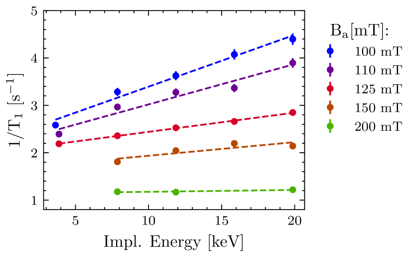
(a) “baseline” sample.

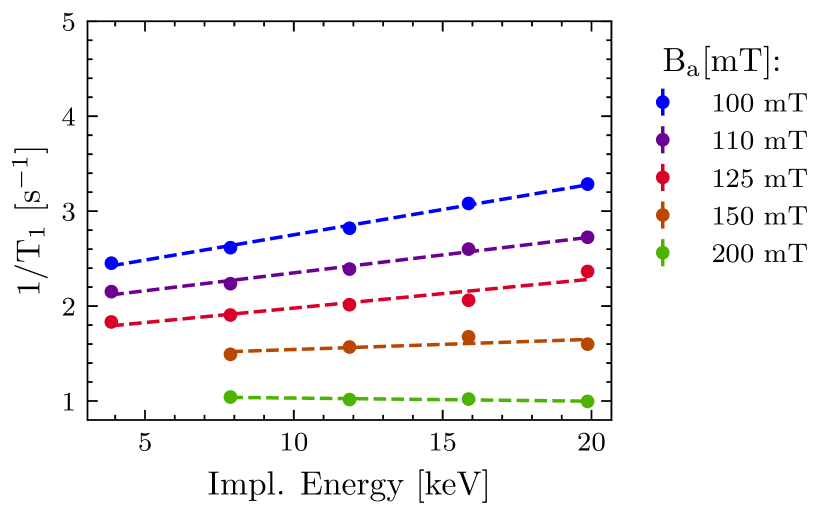
(b) “O-doping” sample.

Figure 1: SLR rate for two Nb samples at various applied fields, $B_{\text{a}}$, as a function of implantation energy. The dashed lines are simple linear fits to the measured relaxation rate to help guide the eye. The diminishing slope as $B_{\text{a}}$ increases indicates the evolution from the Meissner state to the mixed state.

A useful approximation to allow mapping $1/T_{1}\,$ to the average local magnetic field is through a simple Lorentzian model (see e.g., [41]):

$$\frac{1}{T_{1}(E)}\approx\frac{a}{b+\langle B(E)\rangle^{2}},$$ (1)

where $E$ is the implantation energy, $\langle B(E)\rangle$ is the average measured local magnetic field, and $a$ and $b$ are material dependent fit parameters. The $1/T_{1}\,$ values can be explicitly mapped to $\langle B(E)\rangle$ values by using a subset of the datapoints as a basis. The data is taken at a constant temperature (at T$\sim 4.5\text{\,}\mathrm{K}$) to remove any temperature dependence in the Lorentzian fit parameters. The basis points include the $100\text{\,}\mathrm{mT}$ case where the material is expected to be in the Meissner state and the $200\text{\,}\mathrm{mT}$ case where the field is assumed to be fully in the normal state near $B_{c2}$ (for $T\sim$4.5\text{\,}\mathrm{K}$)$. The analysis follows an ansatz approach where a Meissner screening profile is assumed for $100\text{\,}\mathrm{mT}$ and the best fit to a Lorentzian is calculated by varying parameters $a$ and $b$. A single exponential screening profile with some non-superconducting “dead layer” is assumed for the Meissner state as:

$$B(x) =\begin{cases}B_{0}&\text{for $x\leq d$,}\\ B_{0}\exp{-(x-d)/\Lambda}&\text{for $x>d$}\end{cases}$$ (2)

where $B_{0}$ is the field at the surface, $d$ is the “dead layer” in which there is no Meissner screening [42, 43, 44], and $\Lambda$ is the length scale parameter for the exponential decay.

Due to the finite volume of the sample, flux expulsion due to the superconducting diamagnetism enhances the field at the surface of the sample, $B_{0}$, with respect to the applied field ($B_{\text{a}}$) by a factor $\mathcal{E}$ such that $B_{0}=\mathcal{E}B_{\text{a}}$. For our sample geometries, the enhancement factor in the Meissner phase, $\mathcal{E}_{M}$, is determined using the finite element software CST Studio Suite® [45] where the sample is assumed to be perfectly diamagnetic. The average value of the enhancement is determined by averaging over the Gaussian beam spot of the ^8Li^+ ions with typical size of $\sim 4\text{\,}\mathrm{mm}$ in diameter [33]. The sample dimensions and enhancement factors for the Meissner state for each sample are summarized in ’Methods: Sample Preparations’. For the $100\text{\,}\mathrm{mT}$ case, $B_{0}=\mathcal{E}_{M}B_{\text{a}}$ is assumed in the fit. For the applied field of $200\text{\,}\mathrm{mT}$, the diamagnetic field enhancement is expected to be negligible as evidenced by the flat $1/T_{1}\,$ dependence on implantation energy and so, $\mathcal{E}=1$ is assumed in the fit.

The average field sampled by the ^8Li probes for a given implantation energy is a function of the implantation depth distribution, $\rho_{E}(x)$, and the depth profile $B(x)$. For any particular profile, we can calculate a single value of $\langle B(E)\rangle$ as a function of energy via:

$$\langle B(E)\rangle =\int B(x)\rho_{E}(x)dx,$$ (3)

where the Monte Carlo code SRIM [46] is used to calculate the depth distributions at various beam energies (see ‘Methods: Data Analysis’).

The Meissner state screening profile, defined by parameters $\Lambda$ and $d$, and the Lorentzian parameters $a$ and $b$ are varied to give the best fit of the [list-units = single]100;200 $1/T_{1}\,$ values using the Lorentzian function in eq. 1. Assuming $\langle B(E)\rangle$ (in ) and $1/T_{1}\,$ (in ), the best fit ($a$, $b$) parameter values are ($63\,200\pm 1900.\text{\,}$ ,$13\,300\pm 1100.\text{\,}$) and ($50\,600\pm 1300.\text{\,}$, $10\,000\pm 1000.\text{\,}$) for the “baseline” and “O-doping” sample, respectively. The Lorentzian parameters are then used to map the remainder of the $1/T_{1}\,$ data to $\langle B(E)\rangle$. The simple mapping results in the energy dependent screening profiles shown in fig. 2. Here, we note the evident screening at lower applied fields that systematically evolves to no screening as the applied fields increase to $200\text{\,}\mathrm{mT}$. Also note the distinctly different screening profiles between the two samples.

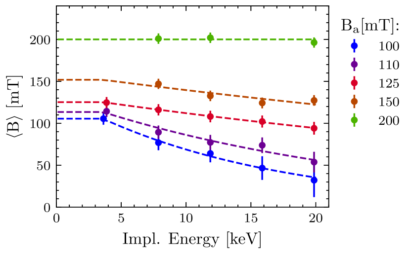
(a) “baseline” sample

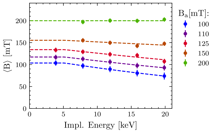
(b) “O-doping” sample

Figure 2: Shown are the average B-field as a function of implantation energy for various applied parallel fields $B_{\text{a}}$ for the two samples. Dashed lines are fits to the data assuming a single exponential function and “dead layer”.

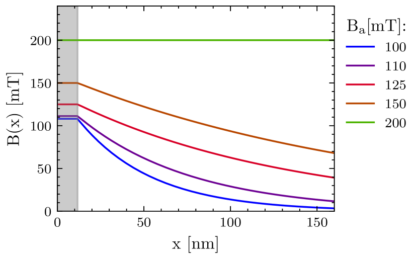
(a) “baseline” sample.

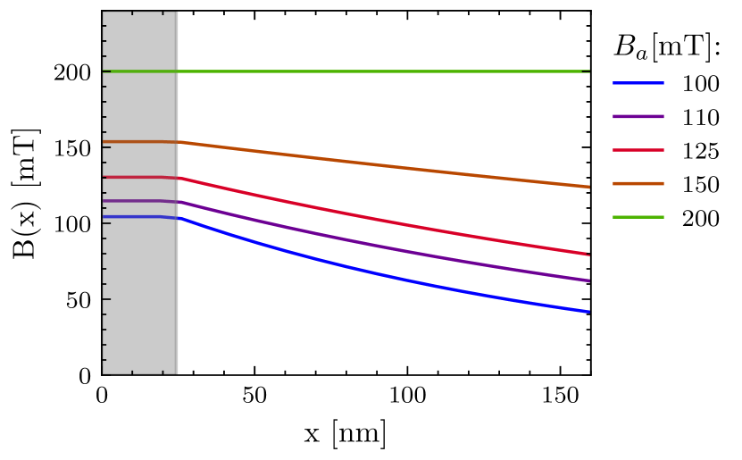
(b) “O-doping” sample.

Figure 3: Extracted field profiles within the first $150\text{\,}\mathrm{nm}$ of the sample surface as a function of $B_{\text{a}}$. The shaded area indicates the non-superconducting “dead layer”.

A more involved analysis is used to extract values of the screening length as a function of applied field. The analysis assumes: 1) a more detailed expression for the relaxation rate which takes into account the dipole-dipole interaction between two different nuclear spins (i.e., the probe ^8Li and the host ^93Nb nuclear spins) [40, 47] as described in ‘Methods: Data Analysis’; and 2) that $1/T_{1}\,$ values are calculated not via the average field, but via the actual field at each depth. The latter is a more accurate technique, but it does not allow a direct mapping of $1/T_{1}\,$ data to an energy dependent screening profile as afforded by the analysis used to produce fig. 2.

As with the previous technique, the 100 and 200 datasets (using the single exponential screening model in eq. 2 and the expected surface field enhancement factors for an applied field of 100 ) are used to establish the Lorentzian-like parameters, now $B_{d}$ and $\tau_{c}$ from eq. 18. The obtained $B_{d}$ and $\tau_{c}$ parameters are then used to extract the best fit for all datasets at various applied fields, $B_{\text{a}}$. We further introduce the normalized enhancement factor, $\mathcal{N}(B_{a})$, that relates the enhancement of the surface field compared to the applied field relative to the sample dependent maximum enhancement factor, $\mathcal{E}_{M}$, in the Meissner state. The normalized enhancement factor is defined through the relation:

$$\mathcal{N}(B_{a})=\frac{\mathcal{E}(B_{\text{a}})-1}{\mathcal{E}_{M}-1}.$$ (4)

For any superconducting volume regardless of its specific dimensions, the normalized enhancement factor should decrease from 1 when the sample is completely in the Meissner phase, to zero in the normal state. For values in between the two limits, the volume exhibits some diamagnetic character. In our analysis, $\mathcal{N}=1$ is assumed for an applied field of $100\text{\,}\mathrm{mT}$ and $\mathcal{N}=0$ for an applied field of $200\text{\,}\mathrm{mT}$. For other applied fields, the data is used to extract $\mathcal{N}$.

Two approaches are used in the fits. In the first case, Case A, the single exponential screening profile that decays to zero, eq. 2, is used for all applied fields. This profile coincides with what we would expect from Meissner screening. In the Meissner state, the value of the normalized enhancement factor should be $\mathcal{N}$=1 and the extracted value of $\Lambda$ corresponds to the magnetic penetration depth $\lambda$. However, once flux begins to break into the sample, the local field is a superposition of an exponentially decreasing field due to the screening currents and an exponentially rising field from the internal vortex distribution (see fig. 4(b)). The latter increases from zero at the surface towards the average bulk equilibrium value of the internal vortices near the surface [48, 49]. The resulting field profile remains a single exponential, but instead of decaying to zero it reduces to the bulk equilibrium value. Therefore, once in the mixed state the Case A analysis outputs an extracted $\Lambda$ that is larger than $\lambda$, and the extracted enhancement factor underestimates the actual enhancement factor.

A second analysis, Case B, is used to better characterize the screening profile in the mixed state. Applied fields that yield a decrease of normalized enhancement factor $\mathcal{N}$ from unity and an abrupt increase in screening length $\Lambda$ in Case A are interpreted as indicating the presence of a mixed state and the screening profile is modified to [49, 50]:

$$B_{\text{Tot}}(x) =\begin{cases}B_{0}&\text{for $x\leq d$,}\\ B_{\rm M}(x)+B_{\rm v}(x)&\text{for $x>d$,}\\ \qquad=B_{0}\exp{-(x-d)/\lambda}+B_{\rm in}\left[1-\exp{-(x-d)/\lambda}\right]\\ \qquad=(B_{0}-B_{\rm in})\exp{-(x-d)/\lambda}+B_{\rm in},\end{cases}$$ (5)

where $B_{\rm M}$ ($B_{\rm v}$) is the Meissner (vortex) contribution to the field profile, $B_{\rm in}$ is the equilibrium field inside the bulk due to vortex entry, and the extracted characteristic length, $\lambda$, is the magnetic penetration depth. In order to minimize the number of fit parameters added to take into account vortex penetration, the applied field, $B_{\text{a}}$, and the interior field, $B_{\rm in}$, are related through the normalized enhancement factor as $B_{\rm in}/B_{\text{a}}=1-\mathcal{N}$. This simple relation is derived from the boundary condition between vacuum and superconductor layer assuming a constant effective magnetization in the volume probed by the beam (see Supplementary Information: ‘Derivation of $B_{\rm in}$’).

The reconstructed field profiles $B(x)$ at increasing $B_{\text{a}}$ are shown in fig. 3 for Case A. The extracted fit outputs for Case A and Case B are summarized in table 1 and table 2 for “baseline” and “O-doping” samples, respectively. The fit outputs, as defined in eq. 2 and eq. 5, include the screening profile length constant ($\Lambda$ in Case A, or $\lambda$ in Case B), the surface field ($B_{0}$), and the normalized enhancement factor ($\mathcal{N}$), all as a function of applied field for each sample. We also introduce the normalized screening depth, defined as the screening characteristic depth normalized to the value at $100\text{\,}\mathrm{mT}$, i.e., $\Lambda_{N}=\Lambda(B_{a})/\Lambda(100$). The plots of $\mathcal{N}$ vs. $B_{a}$ and $\Lambda_{N}$ vs. $B_{a}$ are shown in fig. 4(a) for both samples and for each case. Note that the same values of $\mathcal{N}(B_{a})$ are obtained for both Case A and Case B for the “O-doping” sample. At $B_{\text{a}}=$$150\text{\,}\mathrm{mT}$, despite the different $\Lambda$s obtained for the two cases, the resulting field profiles are virtually identical. For cases where the obtained best fit $\mathcal{N}$ values are not at the lower (i.e., $\mathcal{N}=0$) or upper (i.e., $\mathcal{N}=1$) bound, accurate error estimates of $\mathcal{N}$ can be obtained. They are shown in tables 1 and 2 and in fig. 4(a).

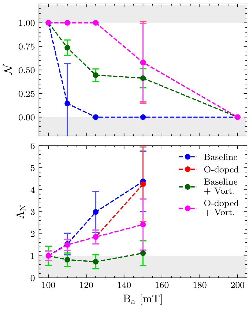
(a)

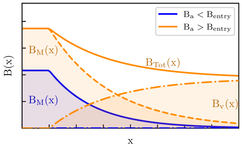
(b)

Figure 4: (a) Normalized surface field enhancement factor $\mathcal{N}$ and normalized screening length $\Lambda_{N}$ for the two samples and for each analysis case (Case A, without vortex, and Case B, with vortex, as described in the text) as a function of the applied field. (b) Expected screening profile from the Meissner ($\rm B_{M}$), vortex ($\rm B_{v}$), and total ($\rm B_{Tot}$) contributions for $B_{\text{a}}<B_{\text{entry}}$ (Meissner state) and for $B_{\text{a}}>B_{\text{entry}}$ with $B_{\rm in}<B_{\text{a}}$ in a mixed state with uniform vortex density.

$B_{\text{a}}$ []	Case A				Case B
	$B_{0}$ []	$\mathcal{N}(B_{a})$	$\Lambda$ []	$\Lambda_{N}$	$B_{0}$ []	$\mathcal{N}(B_{a})$	$\lambda$ []	$\Lambda_{N}$
100	108.1	1	$42.8(13.2)\text{\,}$	$1.0(0.4)\text{\,}$	108.1	1	$42.8(13.2)\text{\,}$	$1.0(0.4)\text{\,}$
110	$111.3(3.8)\text{\,}$	$0.14(0.42)\text{\,}$	$65.6(5.6)\text{\,}$	$1.5(0.5)\text{\,}$	$116.6(0.7)\text{\,}$	$0.74(0.08)\text{\,}$	$35.1(7.4)\text{\,}$	$0.8(0.3)\text{\,}$
125	125	$0\text{\,}$	$127.8(6.0)\text{\,}$	$3.0(0.9)\text{\,}$	$129.5(0.7)\text{\,}$	$0.45(0.07)\text{\,}$	$31.2(9.7)\text{\,}$	$0.7(0.3)\text{\,}$
150	150	$0\text{\,}$	$187.3(10.7)\text{\,}$	$4.4(1.4)\text{\,}$	$155.0(1.2)\text{\,}$	$0.41(0.10)\text{\,}$	$47.9(19.0)\text{\,}$	$1.1(0.6)\text{\,}$
200	200	0	$\infty$	$\infty$	200	0	$\infty$	$\infty$

Table 1: Extracted fit parameters from the $B(x)$ model for the “baseline” sample, measured at $\sim 4.5\text{\,}\mathrm{K}$. The thickness of the “dead layer” is estimated at $d=$$11.7(2.9)\text{\,}\mathrm{nm}$.

$B_{\text{a}}$ []	$B_{0}$ []	$\mathcal{N}(B_{a})$	Case A		Case B
			$\Lambda$ []	$\Lambda_{N}$	$\lambda$ []	$\Lambda_{N}$
100	104.3	1	$146.9(22.6)\text{\,}$	$1.0(0.2)\text{\,}$	$146.9(22.6)\text{\,}$	$1.0(0.2)\text{\,}$
110	114.7	1	$219.8(14.3)\text{\,}$	$1.5(0.3)\text{\,}$	$219.8(14.3)\text{\,}$	$1.5(0.3)\text{\,}$
125	130.4	1	$272.5(19.4)\text{\,}$	$1.9(0.3)\text{\,}$	$272.5(19.4)\text{\,}$	$1.9(0.3)\text{\,}$
150	$153.8(2.8)\text{\,}$	$0.58(0.42)\text{\,}$	$624.7(229.0)\text{\,}$	$4.3(1.7)\text{\,}$	$355.2(161.4)\text{\,}$	$2.4(1.2)\text{\,}$
200	200	0	$\infty$	$\infty$	$\infty$	$\infty$

Table 2: Extracted fit parameters from the $B(x)$ model for the “O-doping” sample, measured at $\sim 4.5\text{\,}\mathrm{K}$. The thickness of the “dead layer” is estimated at $d=$$24.4(11.2)\text{\,}\mathrm{nm}$.

Discussion

The results reveal several notable features. They are: 1) the screening length in the “O-doping” sample is $\sim 3$ times longer than in the “baseline” sample; 2) the screening length in the “O-doping” sample increases significantly as the applied field is increased; 3) flux-penetration into the bulk occurs at a lower field in the “baseline” treatment than in the “O-doping” sample; and 4) the “O-doping” sample possesses a larger non-superconducting “dead layer” than the “baseline” sample.

First, the “O-doping” sample has a significantly larger penetration depth compared to the “baseline” . This is consistent with the expectation that mid-T baking ($400\text{\,}\mathrm{\SIUnitSymbolCelsius}$ for $3\text{\,}\mathrm{h}$) renders a “dirtier” (shorter mean free path) subsurface due to native oxide (Nb2O5) dissolution and interstitial oxygen diffusion [16, 21, 37]. In contrast, the “baseline” sample has a much shorter penetration depth in the Meissner phase consistent with a cleaner Nb surface.

In type-II superconductors, the mixed state transitions to the normal state and the superconducting screening collapses at $B_{c2}(t)$ with temperature dependence [51, 52]:

$$b_{c2}=\frac{1-t^{2}}{1+t^{2}},$$ (6)

where $t=T/T_{c}(B=0)$ is the reduced temperature and $b_{c2}=B_{c2}(T)/B_{c2}(T=0)$ is the reduced upper critical field at temperature $T$. The relation in eq. 6 can be inverted to give the reduced critical temperature at a reduced field $b=B_{0}/B_{c2}(T=0)$:

$$t_{c2} =\sqrt{\frac{1-b}{1+b}},$$ (7)

where $t_{c2}=T_{c2}(B_{0})/T_{c2}(B=0)$.

The two-fluid model can be used to estimate the effective penetration depth, $\lambda$(0,0), at $T=0$ K and $B\rightarrow 0$ via:

$$\lambda(0,0) =\lambda(t,b)\cdot{\sqrt{1-[t(b)]^{4}}},$$ (8)

where the field-dependence of the penetration depth arises due to the field dependence of $T_{c2}(B_{0})$ with the reduced temperature defined earlier as $t(b)=T/T_{c2}(B_{0})$. In the local limit, the relation between $\lambda(0,0,l)$ and the electron mean-free path ($l$)can be estimated from the relation [8]:

$$\lambda(0,0,l)=\lambda_{L}(T=0)\sqrt{1+\frac{\xi_{0}}{l}}.$$ (9)

where $\lambda_{L}$ is defined as the London penetration depth in the limit of pure ($l\rightarrow\infty$) and local ($\xi_{0}\rightarrow 0$) response and $\xi_{0}$ is the Bardeen-Cooper-Schrieffer (BCS) coherence length [53].

Typical quoted values for clean niobium are $T_{c2}(B=0)$ $\sim 9.2\text{\,}\mathrm{K}$ [52, 23], $B_{c2}(T=0)$ $\sim 410\text{\,}\mathrm{mT}$ [52, 23], $\lambda_{L}$ $\sim 40\text{\,}\mathrm{n}\mathrm{m}$  [54, 55] and $\xi_{0}$=$38\text{\,}\mathrm{n}\mathrm{m}$ [55]. Our “baseline” sample is characterized by a residual resistivity ratio (RRR) =300, corresponding to a mean free path of $l$ $\sim 810\text{\,}\mathrm{nm}$ from the empirical relation: $l\text{[nm]}\approxeq 2.7\cdot\text{RRR}$ [1]. Applying eqs. 6, 7, 8 and 9 for our “baseline” sample with measured values of $\lambda(T=$4.5\text{\,}\mathrm{K}$,B_{0}=$108.1\text{\,}\mathrm{mT}$,l=$810\text{\,}\mathrm{nm}$)=$ $42.8\text{\,}\mathrm{nm}$ gives $\lambda(0,0,l=810)=$ $39.0\text{\,}\mathrm{nm}$ or $\lambda_{L}$=$38.1\text{\,}\mathrm{nm}$ in good agreement with expected values.

The same analysis can also be applied for the “O-doping” sample by using the same input values of $T_{c}=$$9.2\text{\,}\mathrm{K}$, $B_{c2}=$$410\text{\,}\mathrm{mT}$ and $\lambda_{L}=$$38.1\text{\,}\mathrm{nm}$ The experimental value of $\lambda(t,b)=$$146.9\text{\,}\mathrm{nm}$ gives a penetration depth of $\lambda(0,0)=$$134.5\text{\,}\mathrm{nm}$ and a mean free path value of $l=$$3.3\text{\,}\mathrm{nm}$ from eq. 9. Mean free path values of doped Nb have been reported by other studies from fits to RF cavity measurements with values in the range of [range-units=single]4200 [56, 57]. The extracted values here are on the low side of this range, which might indicate additional pollution in the surface layer and/or suppressed $T_{c}$ due to an elevated concentration of oxygen impurities [58, 59]. This latter hypothesis can be used to also look at a second key feature of the data from the “O-doping” sample, the increase in screening length with applied field.

We consider first the break-in field implied by the data. Considering the sample geometry and formulation by Brandt for a sample with rectangular cross-section with side length $c$ in the direction of the applied field and side $a$ as the slab thickness, flux will break into the center of a pin free sample at an applied field of [38]:

$$B_{\text{entry}}=B_{c1}\times\tanh(\sqrt{0.36c/a}).$$ (10)

Using the experimentally measured value of $B_{c1}(0K)$$\approx 174\text{\,}\mathrm{mT}$ [12] and scaling this value to the measurement temperature of $\sim 4.5\text{\,}\mathrm{K}$ using $B_{c1}(T)=B_{c1}(0)[1-(T/T_{c})^{2}]$ [52] gives $B_{c1}$($4.5\text{\,}\mathrm{K}$)$\approx 132\text{\,}\mathrm{mT}$. Noting that the samples are slightly different in shape (see table 3) and applying eq. 10, the entry field would be expected at an applied field of $B_{\text{entry}}$$\sim 113\text{\,}\mathrm{mT}$ in the “baseline” and $B_{\text{entry}}$$\sim 123\text{\,}\mathrm{mT}$ in the “O-doping” sample. In the dirtier “O-doping” sample, we expect that the assumed $B_{c1}$ value is reduced from the clean limit value and so this $B_{\text{entry}}$ value represents an upper bound. There is indication from the normalized enhancement factor fits that flux has broken into the “baseline” sample already at an applied field of $110\text{\,}\mathrm{mT}$ ($\mathcal{N}<1$), but in the “O-doping” case the extracted enhancement factor is consistent with the Meissner state ($\mathcal{N}=1$) for applied fields from [range-units=single]100125 (see fig. 4 (a)).

For the “O-doping” cases, the measured magnetic penetration depth $\lambda$ increases significantly as the surface field nears the boundary of the Meissner state, as shown in fig. 4(a). A way to account for this sharp rise is to consider a suppressed $T_{c}$. A decrease of $T_{c}$ for Nb has been reported due to interstitial oxygen diffusion in Nb [58, 59]. A linear fit to the tabulated values of $T_{c}$ vs O concentration from Koch et al. [58] is approximately given by $T_{c}\approxeq T_{c0}-1.01\cdot x$, where $T_{c0}=$$9.2\text{\,}\mathrm{K}$ is the $T_{c}$ of pure Nb and $x$ is the atomic-% concentration of interstitial oxygen in Nb[58]. From eqs. 8 and 7, and using $T_{c}$ as the free variable with fixed $B_{c2}=$410\text{\,}\mathrm{mT}$$, a best fit to the three points in  fig. 5 is for a suppressed $T_{c}$ $\sim 6.5\text{\,}\mathrm{K}$, with $\lambda(0,0)$$\sim 103\text{\,}\mathrm{nm}$ and $l$ $\sim 6\text{\,}\mathrm{nm}$ obtained from eq. 9 by using the same values of $\lambda_{L}$ and $\xi_{0}$ as inputs. This level of suppression would require an oxygen concentration of a few atomic-%, much higher than typical values quoted for “O-doping” treatments that are $\sim 1/10$-th of this concentration ($\lesssim 0.5$ [at%]) [21, 20]. Alternatively, the strong change in screening profile, assuming $T_{c0}=$$9.2\text{\,}\mathrm{K}$, could also be fit by a suppressed upper critical field with $B_{c2}($0\text{\,}\mathrm{K}$)\sim$230\text{\,}\mathrm{mT}$$, or a combination of suppressed $T_{c}$ and suppressed $B_{c2}$. The simultaneous suppression of $T_{c}$ and $B_{c2}$ can be due to the presence of pair-breaking magnetic impurities (see, e.g., [60, 61, 62]) as observed in experimental measurements (see, e.g., [63]), and is consistent with calculations from the microscopic Eilenberger’s equations [64].

Non-magnetic impurities in current carrying superconductors act as pair breakers, in contrast to their pair conserving nature in zero current, thereby reducing the pair potential $\Delta$ and superfluid density [65, 54, 66, 67]. The dependence of superfluid density on screening currents in the Meissner state contributes to non-linear Meissner screening as $\Delta^{2}(B_{0})\propto n_{s}(B_{0})\propto$1/$\lambda^{2}(B_{0})$ [54, 66]. The non-linear screening adds a field-dependent correction term to the magnetic penetration depth on top of implicit $B_{0}$ dependence via $T_{c2}(B_{0})$ in eq. 8. For s-wave superconductors it is predicted that the penetration depth increases quadratically with field [68, 69]:

$$\lambda_{\text{NLME}}(t,b) =\lambda(t,b)\left[1+\beta(T)\left(\frac{B_{0}}{B_{c}}\right)^{2}\right].$$ (11)

Here, $\lambda(t,b)$, $t$ and $b$ are defined in eq. 8 and $\beta(T)$ is the quadratic prefactor. Ginzburg-Landau theory provides an analytical expression for the prefactor $\beta(T\rightarrow T_{c})$, which depends only on the Ginzburg-Landau parameter $\kappa$ (defined as $\lambda/\xi$ for $T\rightarrow T_{c}$) via the following relation [70, 71]:

$$\beta =\frac{\kappa(\kappa+2^{3/2})}{8(\kappa+2^{1/2})^{2}}.$$ (12)

Typical $\kappa$ values of $1\rightarrow 10$ (i.e., in the dirty limit $\kappa\approx\lambda_{L}/l$) for various levels of doping in niobium give $\beta\sim$0.1. For the range of values reported here, with $B_{c}\sim$$200\text{\,}\mathrm{mT}$, the non-linear Meissner screening should enhance the magnetic penetration depth at $125\text{\,}\mathrm{mT}$ only by <2% above the value at $100\text{\,}\mathrm{mT}$. Our reported difference of almost a factor of two is considerably larger than that.

More extreme variations of the screening profile near $B_{c1}$ could come from additional pair-breaking from magnetic impurities or gap anisotropy, resulting in a subgap state that is phenomenologically modeled by density of states with Dynes broadening [67, 72, 66]. For example, magnetic impurities associated with oxygen vacancies in the native surface oxide of Nb have been revealed by tunneling measurements and have been attributed as an intrinsic component to the residual RF resistance commonly encountered in SRF cavities [73, 74, 75, 76]. These subgap states could result in a stronger non-linear field dependence of the Meissner screening similar to the “extreme non-linear Meissner effect” in the gapless state as reported by Lee et al [77].

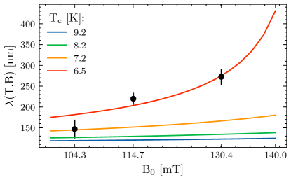
Figure 5: Strong field-dependence of the measured effective magnetic penetration depth (data points) for the “O-doping” sample, compared to a linear Meissner penetration depth model for various reduced critical temperatures $T_{c}$. Note that the penetration depth values are plotted against the surface fields, i.e., $B_{0}=\mathcal{E}B_{\text{a}}$.

Another possible mechanism to partially explain the strong dependence of magnetic penetration depth with applied field near $B_{c1}$ is localized nucleation of vortex loops at the surface [78, 79]. Given the doping used in the “O-doping” sample, it would be expected to have an elevated $\kappa$ and a reduced $B_{c1}$. However, given the observed surface field enhancement (i.e., $\mathcal{N}=1$) which indicates that the bulk of the material remains diamagnetic (see fig. 4(a)), it is likely that the material is operating in a regime above $B_{c1}$ in a meta-stable regime below $B_{sh}$. In this regime, variations in the order parameter from local suppression of $T_{c}$, impurities, inclusions, or field enhancement from surface roughness could suppress locally the superheating barrier and be responsible for the surface nucleation of vortex loops. Such vortices would not penetrate into the bulk, but would increase in number as the applied field is increased, right up to the applied field where flux penetration occurs. These vortex loops at the surface could contribute to the large change in effective penetration depth measured in the doped sample due to the superposition of the Meissner screening profile and the additional surface field from nucleating surface vortices.

Our results in Case B reveal interesting features of the mixed state. As noted in fig. 4(b), after vortices have entered the bulk, the resulting screening profile is a superposition of the exponentially decaying field due to the Meissner screening and the exponentially rising contribution due to the vortex entry that is zero at the surface and rises to the near surface vortex density. While our simple model assumes a uniform flux distribution, the details of the vortex density are defined by the sample geometry [38], the average field in the bulk, the local pinning force [50, 79], as well as additional field dependence of penetration depth $\lambda(B_{\text{a}})$ [65, 80, 67]. Figure 4(a) for Case B indicates that the extracted magnetic penetration depth for the “baseline” sample has a reduced field dependence compared to the “O-doping” sample, consistent with “clean” niobium and a pairing potential that depends only weakly on the applied field. Another interpretation is that some flux may have penetrated the “O-doping” sample giving a non-zero $B_{\rm in}$ (eq. 5), but due to flux pinning the vortices do not redistribute uniformly and remain near the surface after entry. Such an interpretation could be consistent with an increasing screening profile as a function of applied field, but with a surface field enhancement factor $\mathcal{N}\sim 1$. Subsequent studies could be done to evaluate any hysteresis in the screening profile. In general, future experiments could explore near surface magnetic field in the mixed state with more detailed measurements in this field regime.

A notable feature in the data is the shorter “dead layer” in the “baseline” sample ($d$ = $11.7(2.9)\text{\,}\mathrm{nm}$) compared to the “O-doping” sample ($d$ = $24.4(11.2)\text{\,}\mathrm{nm}$). The “dead layer” is a universal feature of all superconductors and is a sample dependent property. The origin of the “dead layer” has previously been attributed to surface roughness (see e.g.[42, 43, 44]). As both samples are from the same batch with the same buffered chemical polishing (BCP) etching step applied, it is unlikely that surface roughness variation is the sole origin of the much larger “dead layer” in the “O-doping” sample. Surface composition characterization has been performed on duplicate witness samples with equivalent treatment using time-of-flight SIMS (TOF-SIMS) and energy dispersive X-ray spectroscopy (EDX), and has been reported by Kolb et al [81]. Both characterizations indicate an elevated level of carbon concentration at the surface of the “O-doping” sample, possibly received during the $400\text{\,}\mathrm{\SIUnitSymbolCelsius}$-bake. The presence of enhanced carbon concentration at the surface is consistent with other studies, e.g., in-situ X-ray photoelectron spectroscopy (XPS), where furnace baking of Nb at $400\text{\,}\mathrm{\SIUnitSymbolCelsius}$ for $3\text{\,}\mathrm{h}$ dissolves the protective Nb2O5 layer below the critical thickness of $1\text{\,}\mathrm{nm}$, thereby promoting surface carbon precipitation [82]. Strong impurity gradients over the first $20\text{\,}\mathrm{n}\mathrm{m}$ have been postulated to modify the magnetic screening profile to non-exponential forms and push peak screening currents away from the surface [83, 84, 85, 37]. Such modified screening profiles with a dead-layer magnitude similar to the “baseline” sample (i.e., $d$$\sim 12\text{\,}\mathrm{n}\mathrm{m}$) may be consistent with our data that we have modeled simply as a single exponential with a larger “dead layer” and enhanced penetration depth. It is also important to note that pair-breaking due to screening currents will vary over the penetration depth $\lambda$. This pair-breaking modifies the super-fluid density locally as a function of the screening depth, i.e., $\Delta[B(x)]^{2}\propto n_{s}(x)\propto$1/$\lambda(x)^{2}$, and therefore results in a non-exponential magnetic screening profile at high field [80].

In summary, the performance of SRF materials near fundamental limits is of critical importance to the accelerator community, as these limits set the scale for the accelerators in terms of operating gradient. Relevant phenomena in this regime have been explored in detail using two heat treated Nb samples, both showing distinct behaviour as a result of their modified subsurface. Theories which self-consistently take into account various pair breaking effects (due to magnetic field, nonmagnetic and magnetic impurities, gap anisotropy, proximity effect from normal metal overlayer) are being extensively developed (see, e.g.,[67, 72, 86, 87, 84, 66, 88]). We anticipate that the $\beta$-SRF facility will be an important tool to validate these proposed theories, and future experiments will help refine our understanding on how to advance and tailor SRF performance.

Methods

Sample Preparations

The sample size is constrained to roughly 10 x 10 x 2 by the mechanical dimensions of the sample ladder in the $\beta$-SRF cryostat [33]. The Nb samples are cutouts of RRR $\gtrsim 300$ Nb sheets sourced from ATI Wah Chang (Albany, Oregon, USA). The samples are prepared simultaneously during processing of bulk Nb RF cavities. All Nb samples first undergo a “baseline” treatment as follows:

1. BCP, a standard chemical etching solution for SRF cavities containing 2:1:1 volume ratio of H3PO4:HNO3:HF, to remove the first $50\text{\,}\mathrm{\SIUnitSymbolMicro m}$ of damaged layers due to cutting/machining. Studies of BCP-treated niobium report typical roughness values of $\sim 1.6\text{\,}\mathrm{\SIUnitSymbolMicro m}$ [89].

2. Annealing in-house with a high-vacuum furnace at $1400\text{\,}\mathrm{\SIUnitSymbolCelsius}$ for $\sim 4\text{\,}\mathrm{h}$ in order to remove pinning sources in the material [12]. During this annealing step, all the samples are wrapped in a clean Nb foil.

3. An additional $5\text{\,}\mathrm{\SIUnitSymbolMicro m}$ BCP is applied to remove possible furnace contaminations.

4. Ultrasound-cleaning with de-ionized water.

A second sample was additionally treated with a “mid-T bake” or “O-doping” recipe where the cavity/sample receives a “bake” of $400\text{\,}\mathrm{\SIUnitSymbolCelsius}$ for $3\text{\,}\mathrm{h}$ under ultra-high vacuum. The dimensions of both “baseline” and “O-doping” samples are shown in table 3 with axis parameters, approximate beam spot size, and applied field orientation defined in fig. 6. Also listed are $\mathcal{E}_{M}$, the Meissner state surface field enhancement factor, and $B_{\text{entry}}$, the expected applied field where flux would break into the sample center, assuming $B_{c1}$=$174\text{\,}\mathrm{m}\mathrm{T}$ at $0\text{\,}\mathrm{K}$.

Parameter	“baseline”	“O-doping”
a ()	1.8	1.7
b ()	9.8	12.4
c ()	8.1	12.6
$\mathcal{E}_{M}$	1.081	1.043
$B_{\text{entry}}$() @ $4.5\text{\,}\mathrm{K}$	113	123

Table 3: Sample dimensions and the calculated geometrical enhancement factor $\mathcal{E}_{M}$ in the Meissner state from finite element simulations and the applied field, $B_{\text{entry}}$, where entry into the bulk is expected.

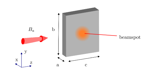
Figure 6: Sample dimensions and orientation with respect to the applied magnetic field and beam implantation. The beamspot is roughly to scale.

$\beta$-NMR Experiment of SRF Samples

The $\beta$-NMR technique [34, 35] implants spin-polarized radioactive ions and measures the local magnetic field at the stopping site of the probe via detection of the emitted $\beta$-particles. The emission of the $\beta$-particles is highly anisotropic and correlated with the direction of the probe’s nuclear spin at the time of the decay. By monitoring the counts of the $\beta$-particles, the local magnetic field can be measured via its influence in reorienting the nuclear spin of the probe. Importantly, $\beta$-NMR provides spatial resolution on the nanometer scale, achieved through the control of the probe’s implantation energy.

The principle of $\beta$-NMR is similar to LE-$\mu$SR [31, 32], but differs in the properties of the probe in use (e.g., radioactive lifetime $\tau$$\sim 1.2\text{\,}\mathrm{s}$ for ^8Li vs $\tau$$\sim 2.2\text{\,}\mathrm{\SIUnitSymbolMicro s}$ for $\mu^{+}$ ). This difference makes the two techniques complementary, as well as allowing different measurements of phenomena occuring over longer timescales. The radioactive ions used in $\beta$-NMR need to be spin-polarized in-flight (via optical pumping), whereas $\mu^{+}$ are intrinsically spin-polarized upon production. A dedicated facility with RIB production, laser polarization, and beam transport is needed before the beam can be delivered to the spectrometer for depth-resolved measurements. The following discussion provides more details on the RIB production, polarization, delivery, and measurements of the $\beta$-NMR facility.

Spin-polarized Probe Production & Beam Transport

High intensity RIBs are routinely produced at the TRIUMF Isotope Separator and Accelerator (ISAC) facility [90] using high-intensity protons from the $500\text{\,}\mathrm{MeV}$ cyclotron as a driver to bombard a solid target. The $\beta$-NMR radioisotope nuclei ^8Li (nuclear spin $I=2$; gyromagnetic ratio $\gamma_{\text{\ch{^8 Li}}}\,/2\pi$ = 6.30198(8) MHz/T [91], electric quadrupole moment $Q$ = $31.4\text{\,}\mathrm{\text{mb}}$ [92]; radioactive lifetime $\tau_{\beta}$ = $\sim 1.21\text{\,}\mathrm{s}$ [93]; and mass $A_{{}^{8}Li}$ = $8.02\text{\,}\mathrm{u}$) are produced with the isotope separation on-line (ISOL) method where they are ionized, extracted, and separated on-line to produce isotopically pure RIBs for various experiments. At the TRIUMF $\beta$-NMR facility, low-energy ([range-units=single]2030) ^8Li^+ ions of $\sim{10}^{7}\text{\,}{\mathrm{s}}^{-1}$ are routinely delivered for experiments [34, 35, 36]. During delivery to the experiment, the ions are neutralized and spin-polarized in-flight at the polarizer facility via collinear optical pumping with circularly polarized resonant laser light [94, 95], yielding a high degree ($\sim 70\text{\,}\mathrm{\char 37\relax}$[96]) of nuclear spin-polarization. They are afterwards re-ionized before delivery to the sample location.

High-parallel-field Spectrometer: “$\beta$-SRF beamline”

The spin-polarized ions can be sent for experiments on either one of two existing beamlines: the $\beta$-NMR beamline with up to $9\text{\,}\mathrm{T}$ applied fields (perpendicular to sample surface & parallel to beam momentum), and the $\beta$-NQR beamline with one spectrometer station capable of fields up to $24\text{\,}\mathrm{mT}$ and a second new spectrometer, highlighted here, capable of $200\text{\,}\mathrm{mT}$ applied fields (each with applied field parallel to the sample surface & transverse to the beam momentum). Each spectrometer is equipped with a magnet coil outside the UHV chamber, a pair of scintillation $\beta$ detectors, an RF coil inside the UHV chamber, and a cold-finger cryostat. The cryostat allows sample cooling down to $\sim 4\text{\,}\mathrm{K}$ and is mounted on an electrically isolated high voltage (HV) platform to allow beam energy deceleration within a short distance from the sample for depth-resolved measurements.

Studies of SRF materials require fields parallel to the sample surface to emulate the RF magnetic field direction with respect to the SRF cavity wall and to provide a uniform surface field over the beamspot. This is challenging to achieve with a low-energy ion beam, due to the strong bending of the beam’s trajectory in this field geometry. To overcome this, a novel beamline extension has been designed and implemented [33], allowing for field strengths of relevance for SRF materials to be employed.

Data Analysis

The local magnetic field profile can be obtained via depth-resolved measurements of the ^8Li SLR rate  [41, 29]. At the TRIUMF $\beta$-NMR facility, the SLR measurements are performed by monitoring the transient decay of the probes’ spin polarization both during and following short pulses of ions (a typical length is $\Delta=$$4\text{\,}\mathrm{s}$). The spin-polarization can be inferred from the $\beta$-rates detected at the two opposing (scintillator) detector pairs. The circular polarization of the pumping laser is typically switched between pulses resulting to alternating parallel (“+”) and anti-parallel (“-”) spin-polarizations to reduce systematic errors. [35, 34] The combined $\beta$-rates (see, e.g.,  [97, 34]) result in the experimental asymmetry which is proportional to the spin-polarization:

$$A(t) =\frac{1-r}{1+r}\equiv A_{0}P(t),\qquad r\equiv\sqrt{\frac{(L_{+}/R_{+})}{(L_{-}/R_{-})}}$$ (13)

where $L_{+/-}$ and $R_{+/-}$ are rates in the opposing counters for the $+/-$ polarization senses, and the initial asymmetry $A_{0}$ depends on the properties of the geometry of the detectors (solid angle) and the intrinsic asymmetry [96, 36].

Once implanted inside the sample, the ions individually interact with the electromagnetic fields of the host lattice and their spins “relax” (depolarize) towards a dynamic equilibrium value while the beam is on, and then towards thermal equilibrium ($\approx 0$) when it is off, with a characteristic SLR relaxation time ($1/T_{1}$). The magnitude of the magnetic field at the implantation site acts to slow the relaxation. Implantation depths can be varied by biasing the sample. By recording the relaxation rates while varying the depth, the applied field, and/or the sample temperature, material properties of interest can be extracted. In order to extract the SLR rate in Nb, the asymmetry spectra are fit to an empirical depolarization function $p(t,t^{\prime};1/T_{1})$, which is convolved with the rectangular beam pulse of length $\Delta$, resulting to a bipartite asymmetry function:

$$A(t) =A_{0}\begin{cases}\cfrac{R_{0}\int_{0}^{t}\exp[-(t-t^{\prime})/\tau]p(t,t^{\prime};1/T_{1})dt^{\prime}}{N(t)}&\text{for $t\leq\Delta$,}\\ \cfrac{R_{0}\int_{0}^{\Delta}\exp[-(t-t^{\prime})/\tau]p(t,t^{\prime};1/T_{1})dt^{\prime}}{N(\Delta)}&\text{for $t>\Delta$,}\end{cases}$$ (14)

$$N(t) =\int_{0}^{t}N(t,t^{\prime})dt^{\prime}=R_{0}\int_{0}^{t}\exp[-(t-t^{\prime})/\tau]dt^{\prime},$$ (15)

where $N(t)$ is the total number of nuclei with mean lifetime $\tau$ that are present at time $t$ after the beam has turned on and implanted at a constant rate $R_{0}$.

The ^8Li^+ depolarization in thin film Nb using a stretched exponential function has been shown to give a good description of ^8Li ’s spin-response at low magnetic fields [47]. The SLR becomes mono-exponential in high applied fields [98]. In our measurements, we note that a small fraction of the ^8Li^+ beam stops in the surrounding cryostat components, necessitating inclusion of an additional “background” term during fitting. This component, however, is small, slow-relaxing, and easily isolated from the signal from the Nb. The total depolarization model (both from the Nb sample and the background signal) can be written as:

$$p_{z}(t,t^{\prime})\approx f_{\ch{Nb}}\exp\left[-\left(\frac{t-t^{\prime}}{T_{1,\ch{Nb}}}\right)^{\beta}\right]+(1-f_{\ch{Nb}})\exp\left[-\left(\frac{t-t^{\prime}}{T_{1,\text{BG}}}\right)\right],$$ (16)

where $f_{\ch{Nb}}$ is the amplitude fraction of the signal from the Nb sample (with values of $f_{\ch{Nb}}$ ranging from 0.82 to 0.94 for “baseline” , and 0.83 to 0.93 for “O-doping” ), $1/T_{1,\ch{Nb}}$ is the relaxation rate of the Nb sample, $1/T_{1,\text{BG}}$ is the relaxation rate of the background (with a value that is shared for all runs in each sample, $1/T_{1,\text{BG}}=0.1$ for “baseline” and $1/T_{1,\text{BG}}=0.06$ for “O-doping” ), and $\beta$ is the stretching exponent (shared for all runs in each sample, $\beta=0.81$ for “baseline” , $\beta=0.89$ for “O-doping” ). The analysis of the asymmetry spectra is performed using the Python application bfit [99] to yield the $1/T_{1}\,$ value for each data set. Examples of the depolarization during beam ON for three different ion energies are shown in fig. 7. The increase in depolarization rate with increasing implantation energy is due to Meissner screening, which reduces the field as a function of depth.

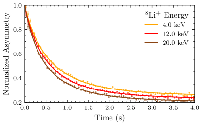
Figure 7: Normalized asymmetry spectra and fits to the data of the Nb components (i.e., with background contributions subtracted) at various implantation energies for the “O-doping” sample at an applied field of $100\text{\,}\mathrm{mT}$ and at $T$$\sim 4.5\text{\,}\mathrm{K}$. The increase in depolarization rate with increasing energy (i.e., subsurface stopping depth) is an indication of Meissner screening.

As summarized in the ‘Results’ section, the analysis employs a direct mapping from the local magnetic field $B(x)$ with a corresponding Larmor frequency $\omega_{i}(x)=\gamma_{i}\ B(x)$, to the local relaxation rate $\frac{1}{T_{1}}(x)$, where $\gamma_{i}$ is the gyromagnetic ratio of the $i$-th nuclear spin (see below). The largest contribution to relaxation at low temperature in the superconducting state and at relatively low applied field ($<1\text{\,}\mathrm{T}$) is due to the dipolar interaction between the ^8Li probe’s nuclear spin $I=2$ and the nuclear spin $S=9/2$ of the 100% abundant host ^93Nb sample [98, 47]. The dipolar relaxation rate resulting from this interaction can be expressed as a weighted sum of three Lorentzian functions, $J_{n}(\omega_{i})$. Each of the Lorentzians is the $n$-quantum spectral density function that models the stochastic fluctuations in the transverse component of the local electromagnetic field. This Lorentzian spectral density function is defined as:

$$J_{n}(\omega_{i}) =\frac{\tau_{c}}{1+\omega_{i}^{2}\tau_{c}^{2}},$$ (17)

where the fit parameter $\tau_{c}$ is an exponential correlation time constant.

The local relaxation rate due to the dipolar interaction can be expressed as [40, 47]:

$$\frac{1}{T_{1}}(x) =\frac{1}{T_{1}}\left[B(x)\right]$$

$$=\gamma_{\text{\ch{^8 Li}}}\,\gamma_{\text{\ch{^{93} Nb}}}\,B_{d}^{2}\left\{\frac{1}{3}J_{0}(\omega_{S}-\omega_{I})+J_{1}(\omega_{I})+2J_{2}(\omega_{S}+\omega_{I})\right\},$$ (18)

where $B_{d}$ is the magnitude of the fluctuating dipolar field at the ^8Li site) and is another fit parameter, $\gamma_{\text{\ch{^8 Li}}}\,$ is the gyromagnetic ratio of the ^8Li probe nuclei, and $\gamma_{\text{\ch{^{93} Nb}}}\,$ ($=2\pi\times$ 10.439565(3388) /) [91] is the gyromagnetic ratio of the ^93Nb host nuclei. To reconstruct the local field, modelled as eq. 2 or eq. 5, we perform a chi-square minimization between the measured SLR rate and an average of the local SLR rate from eq. 18 using the implantation distribution for a given energy:

$$\left\langle\frac{1}{T_{1}}\right\rangle_{E}=\int_{0}^{\infty}\rho_{E}(x)\frac{1}{T_{1}}(x)dx.$$ (19)

Here $\rho_{E}(x)$ is the implantation distribution for ions with implantation energy $E$. These distributions can be accurately simulated using Monte Carlo codes such as SRIM [46] and are shown in fig. 8. The fit to the distribution using a phenomenological distribution function (described in detail in   [47]) is also shown. A $5\text{\,}\mathrm{nm}$ layer of Nb2O5 on a Nb substrate is assumed in the simulation to represent a typical Nb system (see, e.g., [100, 81, 76]).

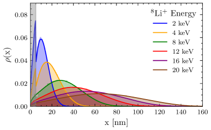
Figure 8: Implantation distributions $\rho(x)$ vs. stopping depth $x$ from SRIM Monte Carlo code [46] simulation, represented as coloured histograms (with 60 bins), for various ^8 Li^+ energies. Solid lines are fits to a phenomenological implantation distribution function (for details, see [47]). The grey area indicates the commonly present Nb2O5 native-oxide layer with typical thickness of $\sim 5\text{\,}\mathrm{nm}$.

Author contributions statement

E.T. and R.E.L. wrote the main manuscript with minor contributions from R.M.L.M. , and all authors reviewed the manuscript. E.T. and P.K. prepared the samples. E.T. , R.E.L. , M.A. , and R.M.L.M. designed the research. E.T. , R.E.L. , J.O.T. , M.A. , S.R.D. , G.D.M. , V.L.K. , D.F. , W.A.M. , R.L. , and S.S. contributed to the $\beta$-NMR measurements. E.T. and R.E.L. performed the analysis. Fitting routines were developed by E.T. and R.E.L. based on original routines developed by R.M.L.M. R.E.L. , T.J. , R.F.K. , and W.A.M. supervise the contributing participants of this experiment. R.E.L. , R.F.K. , and T.J. contribute to the funding acquisition.

Data availability statement

The data and fitting routines supporting the findings of this study are available from the corresponding authors upon reasonable request. Raw data from the $\beta$-NMR experiments (experiment number M1963) are available for download from: https://cmms.triumf.ca.

Additional information

Competing interests: The authors declare no competing financial interests.

References

- [1] Padamsee, H., Knobloch, J. & Hays, T. RF Superconductivity for Accelerators. Wiley Series in Beam Physics and Accelerator Technology (Wiley, 1998).
- [2] Padamsee, H. 50 years of success for SRF accelerators—a review. \JournalTitleSupercond. Sci. Technol. 30, 053003, DOI: 10.1088/1361-6668/aa6376 (2017).
- [3] Padamsee, H. Future Prospects of Superconducting RF for Accelerator Applications. \JournalTitleRev. Accel Sci. Technol. 10, 125–156, DOI: 10.1142/S1793626819300081 (2019).
- [4] Grassellino, A. et al. Nitrogen and argon doping of niobium for superconducting radio frequency cavities: a pathway to highly efficient accelerating structures. \JournalTitleSupercond. Sci. Technol. 26, 102001, DOI: 10.1088/0953-2048/26/10/102001 (2013).
- [5] Gurevich, A. Maximum screening fields of superconducting multilayer structures. \JournalTitleAIP Advances 5, 017112, DOI: 10.1063/1.4905711 (2015).
- [6] Kubo, T. Multilayer coating for higher accelerating fields in superconducting radio-frequency cavities: a review of theoretical aspects. \JournalTitleSupercond. Sci. Technol. 30, 023001, DOI: 10.1088/1361-6668/30/2/023001 (2016).
- [7] Valente-Feliciano, A.-M. Superconducting RF materials other than bulk niobium: a review. \JournalTitleSuperconductor Science and Technology 29, 113002, DOI: 10.1088/0953-2048/29/11/113002 (2016).
- [8] Tinkham, M. Introduction to Superconductivity. Dover Books on Physics Series (Dover Publications, 2004).
- [9] Bean, C. P. & Livingston, J. D. Surface Barrier in Type-II superconductors. \JournalTitlePhys. Rev. Lett. 12, 14–16, DOI: 10.1103/PhysRevLett.12.14 (1964).
- [10] Liarte, D. B. et al. Theoretical estimates of maximum fields in superconducting resonant radio frequency cavities: stability theory, disorder, and laminates. \JournalTitleSuperconductor Science and Technology 30, 033002, DOI: 10.1088/1361-6668/30/3/033002 (2017).
- [11] Prozorov, R., Zarea, M. & Sauls, J. A. Niobium in the clean limit: An intrinsic type-I superconductor. \JournalTitlePhys. Rev. B 106, L180505, DOI: 10.1103/PhysRevB.106.L180505 (2022).
- [12] Junginger, T. et al. Field of first magnetic flux entry and pinning strength of superconductors for rf application measured with muon spin rotation. \JournalTitlePhys. Rev. Accel. Beams 21, 032002, DOI: 10.1103/PhysRevAccelBeams.21.032002 (2018).
- [13] Posen, S., Valles, N. & Liepe, M. Radio frequency magnetic field limits of \chNb and \chNb3Sn. \JournalTitlePhys. Rev. Lett. 115, 047001, DOI: 10.1103/PhysRevLett.115.047001 (2015).
- [14] Watanabe, K., Noguchi, S., Kako, E., Umemori, K. & Shishido, T. Development of the superconducting rf 2-cell cavity for cERL injector at KEK. \JournalTitleNucl. Instrum. Methods Phys. Res., Sect. A 714, 67–82, DOI: 10.1016/j.nima.2013.02.035 (2013).
- [15] Grassellino, A. et al. Accelerating fields up to in TESLA-shape superconducting RF niobium cavities via vacuum bake. Preprint at https://arxiv.org/abs/1806.09824 (2018).
- [16] Ciovati, G. Effect of low-temperature baking on the radio-frequency properties of niobium superconducting cavities for particle accelerators. \JournalTitleJ. Appl. Phys. 96, 1591–1600, DOI: 10.1063/1.1767295 (2004).
- [17] He, F. et al. Medium-temperature furnace baking of 1.3 GHz 9-cell superconducting cavities at IHEP. \JournalTitleSupercond. Sci. Technol. 34, 095005, DOI: 10.1088/1361-6668/ac1657 (2021).
- [18] Posen, S., Transtrum, M. K., Catelani, G., Liepe, M. U. & Sethna, J. P. Shielding Superconductors with Thin Films as Applied to rf Cavities for Particle Accelerators. \JournalTitlePhys. Rev. Applied 4, 044019, DOI: 10.1103/PhysRevApplied.4.044019 (2015).
- [19] Ito, H., Araki, H., Takahashi, K. & Umemori, K. Influence of furnace baking on Q–E behavior of superconducting accelerating cavities. \JournalTitleProg. Theor. Exp. Phys. 2021, DOI: 10.1093/ptep/ptab056 (2021). 071G01.
- [20] Lechner, E. M. et al. SIMS Investigation of Furnace-Baked Nb. In Proc. SRF’21, no. 20 in International Conference on RF Superconductivity, 761–763, DOI: 10.18429/JACoW-SRF2021-THPFDV003 (2022).
- [21] Lechner, E. M. et al. RF surface resistance tuning of superconducting niobium via thermal diffusion of native oxide. \JournalTitleAppl. Phys. Lett. 119, 082601, DOI: 10.1063/5.0059464 (2021).
- [22] Turner, D. A., Burt, G. & Junginger, T. No interface energy barrier and increased surface pinning in low temperature baked niobium. \JournalTitleSci. Rep. 12, 5522, DOI: 10.1038/s41598-022-09023-0 (2022).
- [23] Casalbuoni, S. et al. Surface superconductivity in niobium for superconducting RF cavities. \JournalTitleNucl. Instrum. Methods Phys. Res., Sect. A 538, 45–64, DOI: 10.1016/j.nima.2004.09.003 (2005).
- [24] Balachandran, S. et al. Direct evidence of microstructure dependence of magnetic flux trapping in niobium. \JournalTitleSci. Rep. 11, 5364, DOI: 10.1038/s41598-021-84498-x (2021).
- [25] Wenskat, M. et al. Vacancy-Hydrogen Interaction in Niobium during Low-Temperature Baking. \JournalTitleSci. Rep. 10, 8300, DOI: 10.1038/s41598-020-65083-0 (2020).
- [26] Aull, S. et al. Suppressed Meissner-effect in Niobium: Visualized with polarized neutron radiography. \JournalTitleJournal of Physics: Conference Series 340, 012001, DOI: 10.1088/1742-6596/340/1/012001 (2012).
- [27] Grassellino, A. et al. Muon spin rotation studies of niobium for superconducting rf applications. \JournalTitlePhys. Rev. Spec. Top. Accel Beams 16, 062002, DOI: 10.1103/PhysRevSTAB.16.062002 (2013).
- [28] Romanenko, A. et al. Strong Meissner screening change in superconducting radio frequency cavities due to mild baking. \JournalTitleAppl. Phys. Lett. 104, 072601, DOI: 10.1063/1.4866013 (2014).
- [29] McFadden, R. M. L. et al. Depth-resolved measurements of the Meissner screening profile in surface-treated \chNb. \JournalTitlePhys. Rev. Appl. 19, 044018, DOI: 10.1103/PhysRevApplied.19.044018 (2023).
- [30] Junginger, T., Laxdal, R., MacFarlane, W. A. & Suter, A. SRF material research using muon spin rotation and beta-detected nuclear magnetic resonance. \JournalTitleFrontiers in Electronic Materials 4, DOI: 10.3389/femat.2024.1346235 (2024).
- [31] Prokscha, T. et al. The new E4 beam at PSI: A hybrid-type large acceptance channel for the generation of a high intensity surface-muon beam. \JournalTitleNucl. Instrum. Methods Phys. Res., Sect. A 595, 317–331, DOI: 10.1016/j.nima.2008.07.081 (2008).
- [32] Prokscha, T., Salman, Z. & Suter, A. Low energy SR. In Blundell, S. J., De Renzi, R., Lancaster, T. & Pratt, F. L. (eds.) Muon Spectroscopy: An Introduction, chap. 18, 274–282, DOI: 10.1093/oso/9780198858959.003.0018 (Oxford University Press, Oxford, 2021).
- [33] Thoeng, E. et al. A new high parallel-field spectrometer at TRIUMF’s -NMR facility. \JournalTitleRev. Sci. Instrum. 94, 023305, DOI: 10.1063/5.0137368 (2023).
- [34] MacFarlane, W. A. Implanted-ion NMR: A new probe for nanoscience. \JournalTitleSolid State Nucl. Magn. Reson. 68–69, 1–12, DOI: 10.1016/j.ssnmr.2015.02.004 (2015).
- [35] MacFarlane, W. A. Status and progress of ion-implanted NMR at TRIUMF. \JournalTitleZ. Phys. Chem. 236, 757–798, DOI: doi:10.1515/zpch-2021-3154 (2022).
- [36] Morris, G. D. -NMR. \JournalTitleHyperfine Interact. 225, 173–182, DOI: 10.1007/s10751-013-0894-6 (2014).
- [37] Lechner, E. M. et al. Oxide dissolution and oxygen diffusion scenarios in niobium and implications on the Bean–Livingston barrier in superconducting cavities. \JournalTitleJournal of Applied Physics 135, 133902, DOI: 10.1063/5.0191234 (2024). https://pubs.aip.org/aip/jap/article-pdf/doi/10.1063/5.0191234/19867662/133902_1_5.0191234.pdf.
- [38] Brandt, E. H. Superconductors in realistic geometries: geometric edge barrier versus pinning. \JournalTitlePhysica C 332, 99 – 107, DOI: 10.1016/S0921-4534(99)00651-6 (2000).
- [39] Slichter, C. P. Spin-Lattice Relaxation and Motional Narrowing of Resonance Lines, 145–218 (Springer Berlin Heidelberg, Berlin, Heidelberg, 1990).
- [40] Mehring, M. Principles of High Resolution NMR in Solids (Springer, Berlin, 1983), 2 edn.
- [41] Hossain, M. D. et al. Low-field cross spin relaxation of in superconducting \chNbSe2. \JournalTitlePhys. Rev. B 79, 144518, DOI: 10.1103/PhysRevB.79.144518 (2009).
- [42] Lindstrom, M., Wetton, B. & Kiefl, R. Modelling the effects of surface roughness on superconductors. \JournalTitlePhysics Procedia 30, 249–253, DOI: 10.1016/j.phpro.2012.04.084 (2012). 12th International Conference on Muon Spin Rotation, Relaxation and Resonance (SR2011).
- [43] Lindstrom, M., Wetton, B. & Kiefl, R. Mathematical modelling of the effect of surface roughness on magnetic field profiles in type II superconductors. \JournalTitleJournal of Engineering Mathematics 85, 149–177, DOI: 10.1007/s10665-013-9640-y (2014).
- [44] Lindstrom, M., Y. Fang, A. C. & Kiefl, R. F. Effect of surface roughness on the magnetic field profile in the meissner state of a superconductor. \JournalTitleJ. Supercond. Novel Magn. 29, 1499–1507, DOI: 10.1007/s10948-016-3449-7 (2016).
- [45] CST Studio Suite: Low-frequency Solver, Dassault Systémes.
- [46] Ziegler, J. F., Ziegler, M. D. & Biersack, J. P. SRIM - The stopping and range of ions in matter (2010). \JournalTitleNucl. Instrum. Methods Phys. Res., Sect. B 268, 1818–1823, DOI: 10.1016/j.nimb.2010.02.091 (2010).
- [47] McFadden, R. M. L. et al. Depth-resolved measurement of the Meissner screening profile in a niobium thin film from spin-lattice relaxation of the implanted -emitter \ch^8Li. \JournalTitleJournal of Applied Physics 134, 163902, DOI: 10.1063/5.0175532 (2023).
- [48] Brandt, E. H. Properties of the distorted flux-line lattice near a planar surface. \JournalTitleJournal of Low Temperature Physics 42, 557–584, DOI: 10.1007/BF00117431 (1981).
- [49] Brandt, E. H. Penetration of magnetic ac fields into type-II superconductors. \JournalTitlePhys. Rev. Lett. 67, 2219–2222, DOI: 10.1103/PhysRevLett.67.2219 (1991).
- [50] Xie, W., Liu, Y.-H. & Wen, H.-H. Generalized phenomenological model for the magnetic field penetration and magnetization hysteresis loops of a type-II superconductor. \JournalTitlePhys. Rev. B 105, 014505, DOI: 10.1103/PhysRevB.105.014505 (2022).
- [51] Tinkham, M. Effect of fluxoid quantization on transitions of superconducting films. \JournalTitlePhys. Rev. 129, 2413–2422, DOI: 10.1103/PhysRev.129.2413 (1963).
- [52] Finnemore, D. K., Stromberg, T. F. & Swenson, C. A. Superconducting properties of high-purity niobium. \JournalTitlePhys. Rev. 149, 231–243, DOI: 10.1103/PhysRev.149.231 (1966).
- [53] Bardeen, J., Cooper, L. N. & Schrieffer, J. R. Theory of superconductivity. \JournalTitlePhys. Rev. 108, 1175–1204, DOI: 10.1103/PhysRev.108.1175 (1957).
- [54] Gurevich, A. Theory of RF superconductivity for resonant cavities. \JournalTitleSuperconductor Science and Technology 30, 034004, DOI: 10.1088/1361-6668/30/3/034004 (2017).
- [55] Maxfield, B. W. & McLean, W. L. Superconducting penetration depth of niobium. \JournalTitlePhys. Rev. 139, A1515–A1522, DOI: 10.1103/PhysRev.139.A1515 (1965).
- [56] Maniscalco, J. T., Gonnella, D. & Liepe, M. The importance of the electron mean free path for superconducting radio-frequency cavities. \JournalTitleJournal of Applied Physics 121, 043910, DOI: 10.1063/1.4974909 (2017).
- [57] Koufalis, P. N., Hall, D. L., Liepe, M. & Maniscalco, J. T. Effects of Interstitial Oxygen and Carbon on Niobium Superconducting Cavities. Preprint at https://arxiv.org/abs/1612.08291 (2017).
- [58] Koch, C. C., Scarbrough, J. O. & Kroeger, D. M. Effects of interstitial oxygen on the superconductivity of niobium. \JournalTitlePhys. Rev. B 9, 888–897, DOI: 10.1103/PhysRevB.9.888 (1974).
- [59] DeSorbo, W. Effect of dissolved gases on some superconducting properties of niobium. \JournalTitlePhys. Rev. 132, 107–121, DOI: 10.1103/PhysRev.132.107 (1963).
- [60] Kogan, V. G. & Prozorov, R. Orbital upper critical field of type-II superconductors with pair breaking. \JournalTitlePhys. Rev. B 88, 024503, DOI: 10.1103/PhysRevB.88.024503 (2013).
- [61] Kogan, V. G. & Prozorov, R. Changing the type of superconductivity by magnetic and potential scattering. \JournalTitlePhys. Rev. B 90, 180502, DOI: 10.1103/PhysRevB.90.180502 (2014).
- [62] Kogan, V. G. & Prozorov, R. Critical fields of superconductors with magnetic impurities. \JournalTitlePhys. Rev. B 106, 054505, DOI: 10.1103/PhysRevB.106.054505 (2022).
- [63] Bawa, A., Gupta, A., Singh, S., Awana, V. P. S. & Sahoo, S. Ultrasensitive interplay between ferromagnetism and superconductivity in \chNbGd composite thin films. \JournalTitleSci. Rep. 6, 18689, DOI: 10.1038/srep18689 (2016).
- [64] Eilenberger, G. Transformation of Gorkov’s equation for type II superconductors into transport-like equations. \JournalTitleZ. Phys. A: At. Nucl. 214, 195–213 (1968).
- [65] Lin, F. P.-J. & Gurevich, A. Effect of impurities on the superheating field of type-II superconductors. \JournalTitlePhys. Rev. B 85, 054513, DOI: 10.1103/PhysRevB.85.054513 (2012).
- [66] Gurevich, A. Tuning microwave losses in superconducting resonators. \JournalTitleSuperconductor Science and Technology 36, 063002, DOI: 10.1088/1361-6668/acc214 (2023).
- [67] Kubo, T. Effects of nonmagnetic impurities and subgap states on the kinetic inductance, complex conductivity, quality factor, and depairing current density. \JournalTitlePhys. Rev. Appl. 17, 014018, DOI: 10.1103/PhysRevApplied.17.014018 (2022).
- [68] Yip, S. K. & Sauls, J. A. Nonlinear Meissner effect in \chCuO superconductors. \JournalTitlePhys. Rev. Lett. 69, 2264–2267, DOI: 10.1103/PhysRevLett.69.2264 (1992).
- [69] Xu, D., Yip, S. K. & Sauls, J. A. Nonlinear Meissner effect in unconventional superconductors. \JournalTitlePhys. Rev. B 51, 16233–16253, DOI: 10.1103/PhysRevB.51.16233 (1995).
- [70] Makita, J., Sundahl, C., Ciovati, G., Eom, C. B. & Gurevich, A. Nonlinear Meissner effect in \chNb3Sn coplanar resonators. \JournalTitlePhys. Rev. Res. 4, 013156, DOI: 10.1103/PhysRevResearch.4.013156 (2022).
- [71] Ginzburg, V. L. & Landau, L. D. On the Theory of superconductivity. \JournalTitleZh. Eksp. Teor. Fiz. 20, 1064–1082, DOI: 10.1016/B978-0-08-010586-4.50035-3 (1950).
- [72] Kubo, T. Superheating fields of semi-infinite superconductors and layered superconductors in the diffusive limit: structural optimization based on the microscopic theory. \JournalTitleSuperconductor Science and Technology 34, 045006, DOI: 10.1088/1361-6668/abdedd (2021).
- [73] Proslier, T., Kharitonov, M., Pellin, M., Zasadzinski, J. & Ciovati. Evidence of surface paramagnetism in niobium and consequences for the superconducting cavity surface impedance. \JournalTitleIEEE Trans. Appl. Supercond. 21, 2619–2622, DOI: 10.1109/TASC.2011.2107491 (2011).
- [74] Kharitonov, M., Proslier, T., Glatz, A. & Pellin, M. J. Surface impedance of superconductors with magnetic impurities. \JournalTitlePhys. Rev. B 86, 024514, DOI: 10.1103/PhysRevB.86.024514 (2012).
- [75] Junginger, T., Wasserman, W. & Laxdal, R. E. Superheating in coated niobium. \JournalTitleSupercond. Sci. Technol. 30, 125012, DOI: 10.1088/1361-6668/aa8e3a (2017).
- [76] Wenskat, M. et al. Vacancy dynamics in niobium and its native oxides and their potential implications for quantum computing and superconducting accelerators. \JournalTitlePhys. Rev. B 106, 094516, DOI: 10.1103/PhysRevB.106.094516 (2022).
- [77] Lee, J. E. et al. Gapless superconductivity in \chNb thin films probed by terahertz spectroscopy. \JournalTitleNat. Commun. 14, 2737, DOI: 10.1038/s41467-023-38422-8 (2023).
- [78] Genenko, Y. A., Snezhko, A. V., Troche, P., Hoffmann, J. & Freyhardt, H. C. Magnetic self-field entry into a current-carrying type-II superconductor. III. General criterion of penetration for an external field of arbitrary direction. \JournalTitlePhys. Rev. B 57, 1164–1172, DOI: 10.1103/PhysRevB.57.1164 (1998).
- [79] Asaduzzaman, M., McFadden, R. M. L., Thoeng, E., Laxdal, R. E. & Junginger, T. Measurements of the first-flux-penetration field in surface-treated and coated \chNb: Distinguishing between surface pinning and an interface energy barrier. Preprint at https://arxiv.org/abs/2402.15500 (2024).
- [80] Kubo, T. Superfluid flow in disordered superconductors with dynes pair-breaking scattering: Depairing current, kinetic inductance, and superheating field. \JournalTitlePhys. Rev. Res. 2, 033203, DOI: 10.1103/PhysRevResearch.2.033203 (2020).
- [81] Kolb, P. et al. Mid-T heat treatments on BCP’ed coaxial cavities at TRIUMF. \JournalTitleFrontiers in Electronic Materials 3, DOI: 10.3389/femat.2023.1244126 (2023).
- [82] Prudnikava, A., Tamashevich, Y., Makarova, A., Smirnov, D. & Knobloch, J. In-situ Synchrotron X-Ray Photoelectron Spectroscopy Study of Medium-Temperature Baking of Niobium for SRF Application. Preprint at https://arxiv.org/abs/2312.06529 (2024).
- [83] Checchin, M. & Grassellino, A. High-field Q-slope mitigation due to impurity profile in superconducting radio-frequency cavities. \JournalTitleApplied Physics Letters 117, 032601, DOI: 10.1063/5.0013698 (2020).
- [84] Ngampruetikorn, V. & Sauls, J. A. Effect of inhomogeneous surface disorder on the superheating field of superconducting RF cavities. \JournalTitlePhys. Rev. Res. 1, 012015, DOI: 10.1103/PhysRevResearch.1.012015 (2019).
- [85] McFadden, R. M. L., Asaduzzaman, M. & Junginger, T. Comment on “Strong Meissner screening change in superconducting radio frequency cavities due to mild baking” [Appl. Phys. Lett. 104, 072601 (2014)]. \JournalTitleApplied Physics Letters 124, 086101, DOI: 10.1063/5.0157000 (2024).
- [86] Gurevich, A. & Kubo, T. Surface impedance and optimum surface resistance of a superconductor with an imperfect surface. \JournalTitlePhys. Rev. B 96, 184515, DOI: 10.1103/PhysRevB.96.184515 (2017).
- [87] Kubo, T. & Gurevich, A. Field-dependent nonlinear surface resistance and its optimization by surface nanostructuring in superconductors. \JournalTitlePhys. Rev. B 100, 064522, DOI: 10.1103/PhysRevB.100.064522 (2019).
- [88] Zarea, M., Ueki, H. & Sauls, J. A. Effects of anisotropy and disorder on the superconducting properties of niobium. \JournalTitleFrontiers in Physics 11, DOI: 10.3389/fphy.2023.1269872 (2023).
- [89] Xu, C., Tian, H., Reece, C. E. & Kelley, M. J. Enhanced characterization of niobium surface topography. \JournalTitlePhys. Rev. ST Accel. Beams 14, 123501, DOI: 10.1103/PhysRevSTAB.14.123501 (2011).
- [90] Dilling, J. & Krücken, R. The experimental facilities at ISAC. \JournalTitleHyperfine Interact. 225, 111–114, DOI: 10.1007/s10751-013-0886-6 (2014).
- [91] Stone, N. J. Table of recommended nuclear magnetic dipole moments: Part I — long-lived states. INDC(NDS) 0794, International Atomic Energy Agency, Vienna (2019).
- [92] Stone, N. J. Table of nuclear electric quadrupole moments. INDC(NDS) 0833, International Atomic Energy Agency, Vienna (2021).
- [93] Fléchard, X. et al. Measurement of the \ch^8Li half-life. \JournalTitlePhys. Rev. C 82, 027309, DOI: 10.1103/PhysRevC.82.027309 (2010).
- [94] Levy, C. D. P. et al. Laser polarization facility. \JournalTitleHyperfine Interact. 225, 165–172, DOI: 10.1007/s10751-013-0896-4 (2014).
- [95] Li, R. et al. Recent upgrades and developments at TRIUMF’s laser nuclear-spin-polarization facility. \JournalTitleNucl. Instrum. Methods Phys. Res., Sect. B 541, 228–231, DOI: 10.1016/j.nimb.2023.05.041 (2023).
- [96] MacFarlane, W. A. et al. The Initial State of Optically Polarized \ch^8Li^+ from the -NMR in Bismuth. \JournalTitleJ. Phys. Conf. Ser. 551, 012059, DOI: 10.1088/1742-6596/551/1/012059 (2014).
- [97] Fujimoto, D. Digging Into MUD with Python: mudpy, bdata, and bfit. Preprint at https://arxiv.org/abs/2004.10395 (2020).
- [98] Parolin, T. J. et al. Nuclear magnetic resonance study of \chLi implanted in a thin film of niobium. \JournalTitlePhys. Rev. B 80, 174109, DOI: 10.1103/PhysRevB.80.174109 (2009).
- [99] Fujimoto, D. bfit: A Python Application For Beta-Detected NMR. \JournalTitleJournal of Open Source Software 6, 3598, DOI: 10.21105/joss.03598 (2021).
- [100] Halbritter, J. On the oxidation and on the superconductivity of niobium. \JournalTitleApplied Physics A 43, 1–28, DOI: 10.1007/BF00615201 (1987).
Acknowledgements
The authors of this work would like to thank: M. Cervantes, D. O. Rosales for assistance with sample preparation, as well as TRIUMF CMMS, SRF, DAQ, Operations and Beam Delivery groups for excellent technical support before and during the experiment. Funding was provided through a Research Tools and Infrastructure grant [SAPEQ-2015-00005] and Discovery grant [SAPIN-2019-00040] and [SAPPJ-2020-00030] from the Natural Sciences and Engineering Research Council of Canada (NSERC).